Tracking the Walking Gait of a Novel Quadruped Robot with Soft Actuators Using Model Predictive Control

Abstract

Quadruped robots are used in various scenarios, but their rigid structure limits their applications. In contrast, soft structures offer greater flexibility, adaptability, and lower costs but struggle with motion modeling and control stability. This paper proposes a novel design for a quadruped robot that uses pneumatic soft actuators for joint movement. Firstly, kinematic principles are applied to model single-leg movements; subsequently, a data-driven approach is proposed to model the soft actuator by integrating the control principle with the single-leg structure. Furthermore, a system identification-based approach is proposed for parameter estimation. Ultimately, the model predictive control method is effectively employed to track the predefined gait during locomotion. Experimental results demonstrate that the designed robot can walk smoothly and follow the preset gait accurately.

1. Introduction

Quadruped robots offer a combination of strong stability, high flexibility, and excellent obstacle-crossing abilities [1,2,3]. However, with the growing integration of robots into human society, soft actuators are regarded as a highly promising alternative to rigid structures due to their softness and mechanical compatibility. The application of soft actuators not only reduces the weight of quadruped robots but also enhances their terrain adaptability, thereby improving their ability to navigate through challenging environments [4,5,6,7]. Recently, significant advancements have been made in the field of soft-rigid coupled robotics, with one of the most widely used applications involving the soft transformation of rigid actuators within rigid robotic systems [8,9,10]. When it comes to soft actuators, McKibben artificial muscles are currently among the most widely used fluidic muscles [11]. The mechanism relies on converting the circumferential stress of a pressurized inner tube into axial contraction force via a double helical braided sleeve. The simplicity of this design allows for the easy replication of movements similar to those of skeletal muscles. The University of Texas introduced a ball-socket joint-based artificial musculoskeletal system [12], utilizing 3D printing to fabricate the joints. Muscle actuators composed of resistance wire and silicone were incorporated within four channels of the joints. This system is powered by an electrothermal drive, enabling multi-dimensional movement. Preston Ohta and his team developed a seven-degree-of-freedom bionic robotic arm [13], featuring a rigid carbon fiber composite skeleton. The arm is powered by pneumatic artificial muscles, while the wrist is driven by servos. An airbag sleeve encases the robotic arm to absorb impacts, enhancing the compliance of the pneumatic muscles. Jing proposed a continuous robotic manipulator with a rigid-flexible coupling structure (RFCM) [14], consisting of multiple bellows and a spine-shaped rigid framework. This design improves the manipulator’s rigidity, load-bearing capacity, and vibration resistance.

Notably, research on pneumatic soft robots has achieved remarkable progress in recent years. Ren et al. (2023) designed a gas-driven soft quadruped robot, dividing its leg structure into a cavity structure and a gas actuator, and elaborated on their structural design, material selection, and fabrication methods [15]. They established kinematic models for the robot and completed static and dynamic gait planning based on stability criteria, verifying the effectiveness of the mathematical model through experiments [15]. Zhang (2025) proposed a novel bionic snake-like robot design based on a hexagonal structure, with its body modules composed of hexagonal structures and scales, powered by the interaction between the hexagonal structure, scales, and the ground [16]. The study conducted mathematical modeling and kinematic analysis of the robot’s structure, designed a control system including hardware selection and circuit design, and applied a model identification adaptive control (MIAC) algorithm for motion control, achieving stable movement of the snake-like robot [16]. Additionally, Meng et al. (2024) optimized the actual PID control of walking quadruped soft robots using genetic algorithms and developed a new pneumatic quadruped soft robot based on a honeycomb structure, providing valuable references for the structural design and control strategy of soft quadruped robots [17,18].

In general, incorporating soft actuators into a robot’s rigid framework can greatly improve both its agility and safety. However, soft actuators still face challenges, particularly in modeling, control, and structural stability, which demand more research [19,20,21]. The development of novel structures, precise modeling and control for soft-actuated quadruped robots remain key research difficulties. This study reports the control process of a novel quadruped robot, which uses soft actuators to drive the joints for leg movements. The actuator of each leg features a pneumatic honeycomb structure. Firstly, a gait motion model was established based on the kinematic principle. System identification methods were then used to estimate the parameters of the control model, and model predictive control techniques were subsequently applied to track the preset walking gait. The presented quadruped robot demonstrates robust walking performance and achieves high-precision gait tracking. In contrast to our earlier studies [17,18], which used a different pneumatic configuration and a genetic-algorithm-optimized PID controller, the present work adopts the redesigned honeycomb platform, obtains a data-driven state-space model through system identification, and introduces an MPC gait-tracking controller with explicit input constraints. Recent optimization-based studies have further addressed multi-task coordination and safe motion planning in robotic systems [22], providing a broader background for the present controller design.

2. Structure and Kinematic Analysis

2.1. Robot Structure

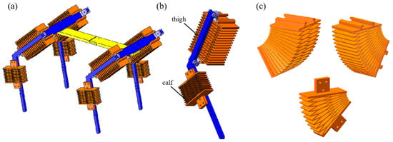
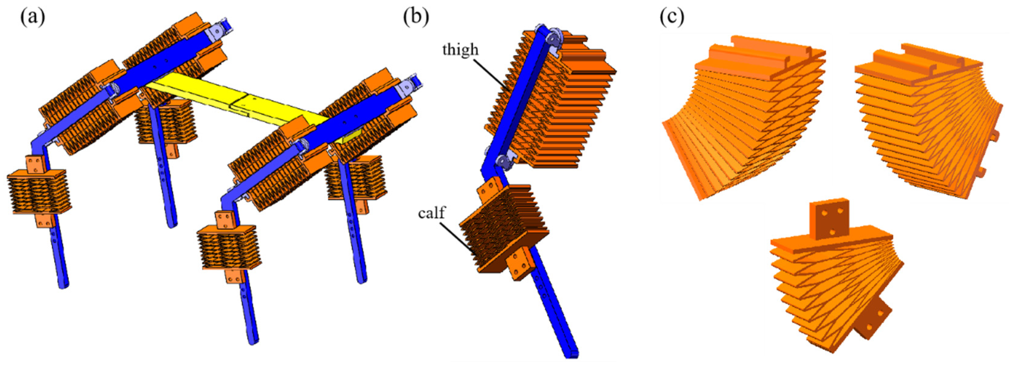
Soft-driven structure: The limbs of the quadruped robot are structured with a three-joint design, consisting of the thigh and shank sections, as shown in Figure 1a. The thigh offers two degrees of freedom, enabling forward, backward, and horizontal movement, while the shank is capable of lateral movement with its one degree of freedom. Each segment is equipped with independent soft pneumatic actuators, as shown in Figure 1b. It is worth noting that the hexagonal structure exhibits remarkable flexibility in deformation in both lateral and longitudinal directions and can be compactly arranged into a honeycomb configuration [23]. Therefore, a pneumatic honeycomb muscle structure was developed to drive the movement of the robot’s limbs based on the deformation and geometric properties of hexagons. The pneumatic actuator for the thigh adopts a double-layer structure, with chambers arranged on either side, while the shank uses a single-layer design. This configuration allows for bidirectional and reversible deformation. The deformation is accomplished by inflating the chambers of the actuator, and different inflation strategies control the actuator’s bending movements. As shown in Figure 1c, the lateral bending of the thigh is achieved by separately inflating the inner and outer sides of the double-layer actuator. Forward and backward bending is realized by inflating the chambers on either the left or right side. Similarly, the shank bends forward or backward as gas fills its structure. The mesh-like structure of the air bands is designed to minimize the number of air holes. Inflation exerts pressure on the inner walls of the chambers. This pressure causes deformation that drives the robot’s leg movement.

Figure 1. The designed soft quadruped robot. (a) Soft quadruped robot structure; (b) single leg structure; (c) bending form of the pneumatic honeycomb structure.

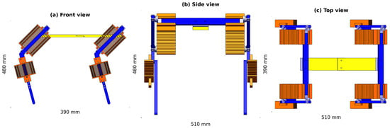
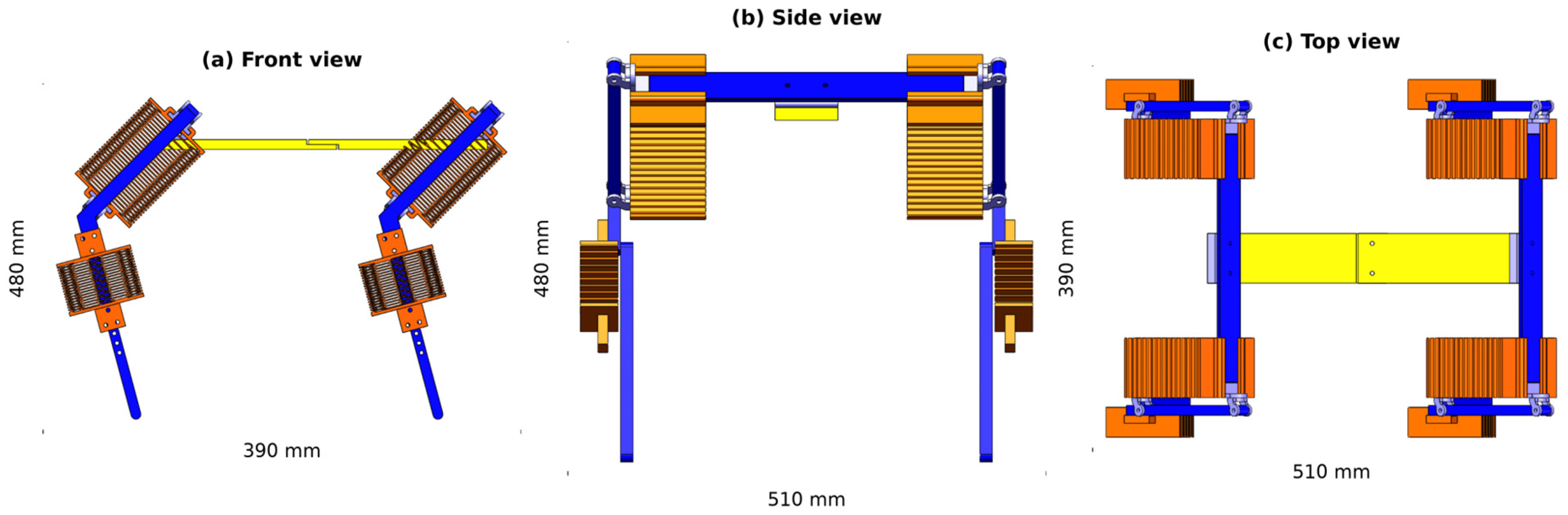
Rigid frame structure: The robot’s form, including its torso, limbs, and joints, is shaped by a rigid framework, as shown in Figure 1a. Based on the joint positions of quadrupeds, the rotational parts of the robot’s leg are referred to as the hip and knee joints, while its limb sections are labeled as thigh and shank. The hip joint permits rotation laterally and front to back, while the knee joint enables forward–backward swinging rotation. The robot’s torso takes on an “I” shape, comprising two identical parts: the shoulder plates that link the limbs and the base that connects the front and hind limbs. As shown in Figure 2, the prototype has overall dimensions of approximately 510 mm (length) × 390 mm (width) × 480 mm (height) in its standing configuration and a total mass of approximately 1.9 kg, including the onboard data-acquisition module.

Figure 2. Overall dimensions of the quadruped robot in the standing configuration: (a) front view, (b) side view, and (c) top view. Overall envelope approximately 510 mm (length) × 390 mm (width) × 480 mm (height).

2.2. Leg Kinematic Analysis

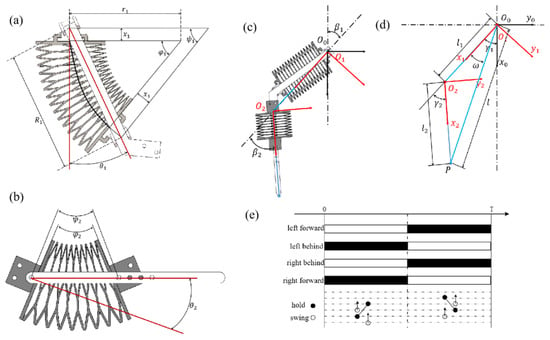
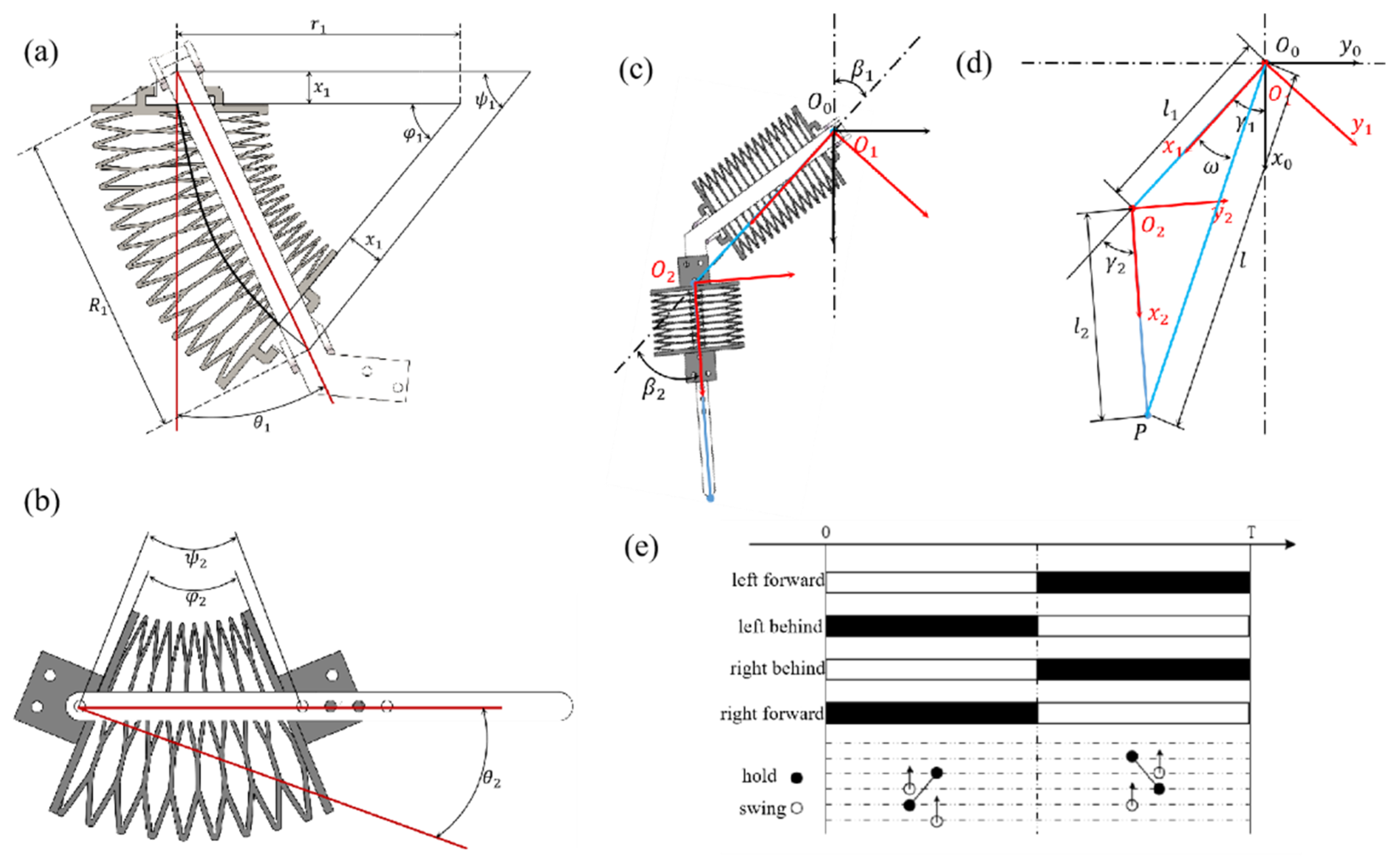
The quadruped robot’s single leg has a three-joint mechanical structure. Soft actuators generate bending deformation, causing the robot’s limbs to swing around the joint axis. The coordinated movement of all limbs enables locomotion. The relationship between the actuator’s bending angle and the leg’s rotational angle is determined geometrically. When the pneumatic honeycomb chambers inflate, the actuators, fixed to the thigh’s rigid structure and connected by rotatable joints, bend without elongation. The soft actuators rotate the rigid structure around the joint axis, creating uniform curvature. The relationship between the thigh’s rotation angle θ₁ and bending angle φ₁, shown in Figure 3a, at the joint is expressed as:

$${\theta }_1=90-{\displaystyle \frac{180-{\psi }_1}{2}}=90-{\displaystyle \frac{180-{\phi }_1}{2}}={\displaystyle \frac{{\phi }_1}{2}}$$

(1)

Figure 3. Leg kinematic analysis: (a) side view of a partially flexed thigh, (b) side view of a partially flexed shank, (c) establishment of the coordinate system for the single-leg model, (d) simplification of the coordinate model, and (e) dynamic walking timing chart.

The rotational angle conversion θ₂ for the shank, shown in Figure 3b, is identical to that of the thigh and can be represented as:

$${\theta }_2=={\displaystyle \frac{{\phi }_2}{2}}$$

(2)

Here, φ₂ represents the angle between the planes at both ends of the shank actuator. The angles between the planes at both ends of the thigh and shank actuators can be measured using bending sensors. Thus, the rotation angles of each soft actuator can be derived according to the above equations.

The robot walks depending on the foot end for movement. Forward kinematic analysis is necessary to deduce the end position of the leg based on the measured angles of the thigh and shank. Since the designed quadruped robot performs a forward gait, the single-leg model is simplified into the X-Y plane, as shown in Figure 3c. Using the D-H notation, the world coordinate system {O₀}, the thigh coordinate system {O₁}, and the shank coordinate system {O₂} are established, as shown in the figure. l₁ represents the distance from the hip joint’s rotational axis to the knee joint’s rotational axis. l₂ represents the distance from the knee joint’s rotational axis to the foot endpoint, denoted as point P. γ_i (i = 1, 2) indicates the joint rotation angles. β₁ and β₂ are the initial angles of the thigh and shank when the robot is positioned. The transformation matrix from the shank coordinate system {O₂} to the world coordinate system {O₀} is expressed as follows: For the forward straight-line gait considered in this work, the lateral hip motion is constrained by the torso frame and by the diagonal-leg walking sequence, so each leg moves essentially in its sagittal plane and can be described by the two joint rotation angles γ1 (thigh) and γ2 (shank); the neglected lateral degree of freedom is left as a future extension.

$${}_2{}^{0}T=\left[\begin{array}{cccc}\cos {\gamma }_1\cos {\gamma }_2-\sin {\gamma }_1\sin {\gamma }_2& -\cos {\gamma }_1\sin {\gamma }_2-\sin {\gamma }_1\cos {\gamma }_2& 0& l_1\cos {\gamma }_1\\ \sin {\gamma }_1\cos {\gamma }_2+\cos {\gamma }_1\sin {\gamma }_2& -\sin {\gamma }_1\sin {\gamma }_2+\cos {\gamma }_1\cos {\gamma }_2& 0& l_1\sin {\gamma }_1\\ 0& 0& 1& 0\\ 0& 0& 0& 1\end{array}\right]$$

(3)

The pose coordinate of the foot endpoint in the shank coordinate system is:

$${}^{2}P=\left[\begin{array}{cccc}{l}_2& 0& 0& 1\end{array}\right]$$

(4)

The pose coordinates of point P in the world coordinate system is:

$${}^{0}P={}_2{}^{0}T{}^{2}P=\left[\begin{array}{c}{l}_2\cos {\gamma }_1\cos {\gamma }_2-l_2\sin {\gamma }_1\sin {\gamma }_2+l_1\cos {\gamma }_1\\ l_2\sin {\gamma }_1\cos {\gamma }_2+l_2\cos {\gamma }_1\sin {\gamma }_2+l_1\sin {\gamma }_1\\ 0\\ 1\end{array}\right]$$

(5)

The relationship between θ_i and β_i can be expressed as:

$${\theta }_i=\gamma {}_i-{\beta }_i$$

(6)

The relationship between the coordinates of P and θi can be obtained using Equations (5) and (6). Here, li and β1 are fixed parameters that can be pre-measured, and θ1 is a parameter that can be measured using bending sensors.

In practical applications, the designed robot needs to follow a predetermined trajectory, and the joint rotation angles need to be known in advance from the known endpoint positions. Thus, inverse kinematics analysis is required. Analytical methods are used to solve the inverse kinematics of a single robot leg [24]. In Figure 3d, the simplified model of a single leg defines the counterclockwise direction as positive. The coordinates of the robot’s endpoint P in the world coordinate system {O₀} are assumed to be (x, y, z). When the mechanical leg swings back and forth, the vertical coordinate z of point P remains at 0. Therefore, the distance l from point P to the origin of the coordinate system {O₀} is:

$$l=\sqrt{x^2+y^2}$$

(7)

γ₂ is represented as:

$${\gamma }_2=\arccos ({\displaystyle \frac{x^2+y^2-l_1^2-l_2^2}{2l_1{l}_2}})$$

(8)

ω can be calculated according to geometric relationships as:

$$\omega =\arccos ({\displaystyle \frac{l_1^2+x^2+y^2-l_2^2}{2l_1\sqrt{x^2+y^2}}})$$

(9)

Therefore, γ₁ can be expressed as:

$${\gamma }_1=\arctan {\displaystyle \frac{y}{x}}-\omega$$

(10)

Equation (6) reveals the relationship between γi and θi. The relationship between the bending angle θi for the thigh and shank and the coordinates of the endpoint P can be established by combining Equation (6) and Equation (10).

After completing the modeling, gait planning is performed. Various quadruped animals form different gaits through the coordinated movement of their four legs. Their walking methods offer valuable references for quadruped robot locomotion. Currently, researchers commonly use two types of gaits in robots: static and dynamic walking. Dynamic walking is a faster gait where forward is defined as positive. In this walking mode, the diagonal pairs of legs have no time phase difference. Figure 3e illustrates the timing diagram for dynamic walking. The four legs swing forward in a cyclic order according to a predetermined sequence. At every moment during the motion cycle, the foot ends of two legs are on the ground, providing support, while the foot ends of the other two legs are lifted and move forward.

3. Model and Control for Soft Actuator

3.1. Data-Based Model

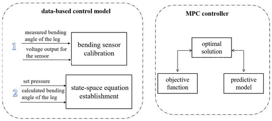
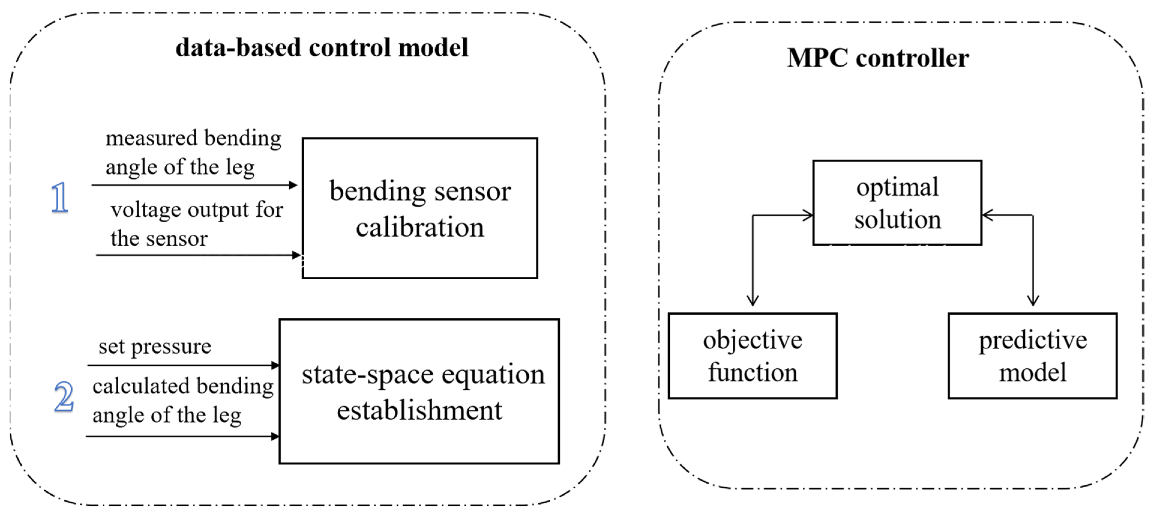
The modeling and control of the soft actuator present significant challenges. As shown in Figure 4, this paper proposes a data-driven modeling approach. The control modeling of the robot’s soft actuator is conducted based on input and output data. The input signal {x(t)} denotes the air pressure injected into the soft actuator, and the output signal {y(t)} represents its bending angle. The bending sensor is affixed to the side of the soft actuator, with its voltage signal variations reflecting the bending angle. Thus, each bending sensor can derive the rotation angle of the leg from the voltage signal after sensor calibration. This paper uses system identification to establish the control model. This modeling approach simplifies the control model of the soft structure and can be effectively integrated with control methods. The state-space equation of the model is as follows:

$$\left\{\begin{array}{c}\mathit{dx}/\mathit{dt}=\mathit{Ax}(t)+\mathit{Bu}(t)\\ y(t)=\mathit{Cx}(t)+\mathit{Du}(t)\end{array}\right.$$

(11)

where A, B, C, D are parameter matrices in the equation system. Their specific values can be calculated by fitting the input and output data with a third-order model. In the identification experiment, the actuator was excited by a repeated square-wave voltage signal (amplitude +/−1.5 V to +/−2.5 V), sampled at 50 Hz. The input was the proportional-valve command (0–10 V, corresponding to an output pressure of 0.001–0.5 MPa), and the output was the measured bending angle. The third-order model was fitted from the identification data and validated on an independent dataset, achieving fitting accuracies of 95.19% for the thigh and 96.35% for the shank actuator.

Figure 4. Model and control.

3.2. Gait Control

Model predictive control (MPC) is an advanced control strategy that uses a mathematical model of the system to predict future system behavior. It then solves for the optimal control input at each control interval through optimization algorithms [25,26]. In this paper, the system model is represented using state-space equations and applied to the control of the soft actuator. The core highlight lies in first obtaining the state-space equations through data collection and system identification. Equation (11) is then discretized according to the sampling frequency to obtain a discrete state-space model. Thus, the MPC method is successfully applied to the control of the soft actuator. The system output is predicted based on the number of future samples, with a prediction horizon of Np. The sample data within the prediction horizon is then used for output control, with a control horizon of Nc. The control objective is to make the predicted output as close as possible to the set value, which requires finding the optimal control input u. Therefore, the objective function is:

$$\begin{array}{c}J(k)={{\displaystyle \sum _{i=1}^{N_P}\left[\hat{y}(k+i | k)-r(k+i | k)\right]}}^T\cdot Q\cdot \left[\hat{y}(k+i | k)-r(k+i | k)\right]+\\ {\displaystyle \sum _{i=1}^{N_c}\Delta u^T}(k+i-1 | k)\cdot R\cdot \Delta u(k+i-1 | k)\end{array}$$

(12)

where Δu = u(k) − u(k − 1), Q is the output error weight matrix, and R is the input error weight matrix. The state-space equation is a single-input, single-output system. Therefore, Equation (12) can be simplified as follows: The identified third-order model is discretized with the sampling period to give the discrete state-space model x(k + 1) = A_d x(k) + B_d u(k), y(k) = C_d x(k). Over the prediction horizon, the future states and outputs are accumulated into a compact prediction equation Y = Psi x(k) + Phi U. At each control interval, the controller minimizes the quadratic tracking objective subject to the input constraint |u(k + i)| ≤ 3 V; the resulting optimal input sequence is solved online, only its first element is applied to the proportional valve, and the horizon is then recedingly shifted. The prediction and control horizons are set to Np = 30 and Nc = 3, with the output weight Q = 0.1 and the input weight R = 10.

$$J(k)={{\displaystyle \sum _{i=1}^{N_P}\left[\hat{y}(k+i | k)-r(k+i | k)\right]}}^2\cdot q+{\displaystyle \sum _{i=1}^{N_c}\Delta u^T}{(k+i-1 | k)}^2\cdot r$$

(13)

For Equation (13), the derivative is carried out to obtain the optimal solution, which is expressed as:

$${\displaystyle \frac{\partial J}{\partial u}}=0$$

(14)

4. Experiment

4.1. Designed Platform

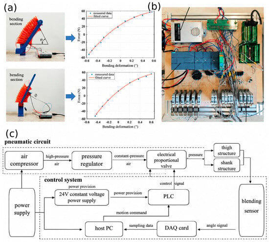
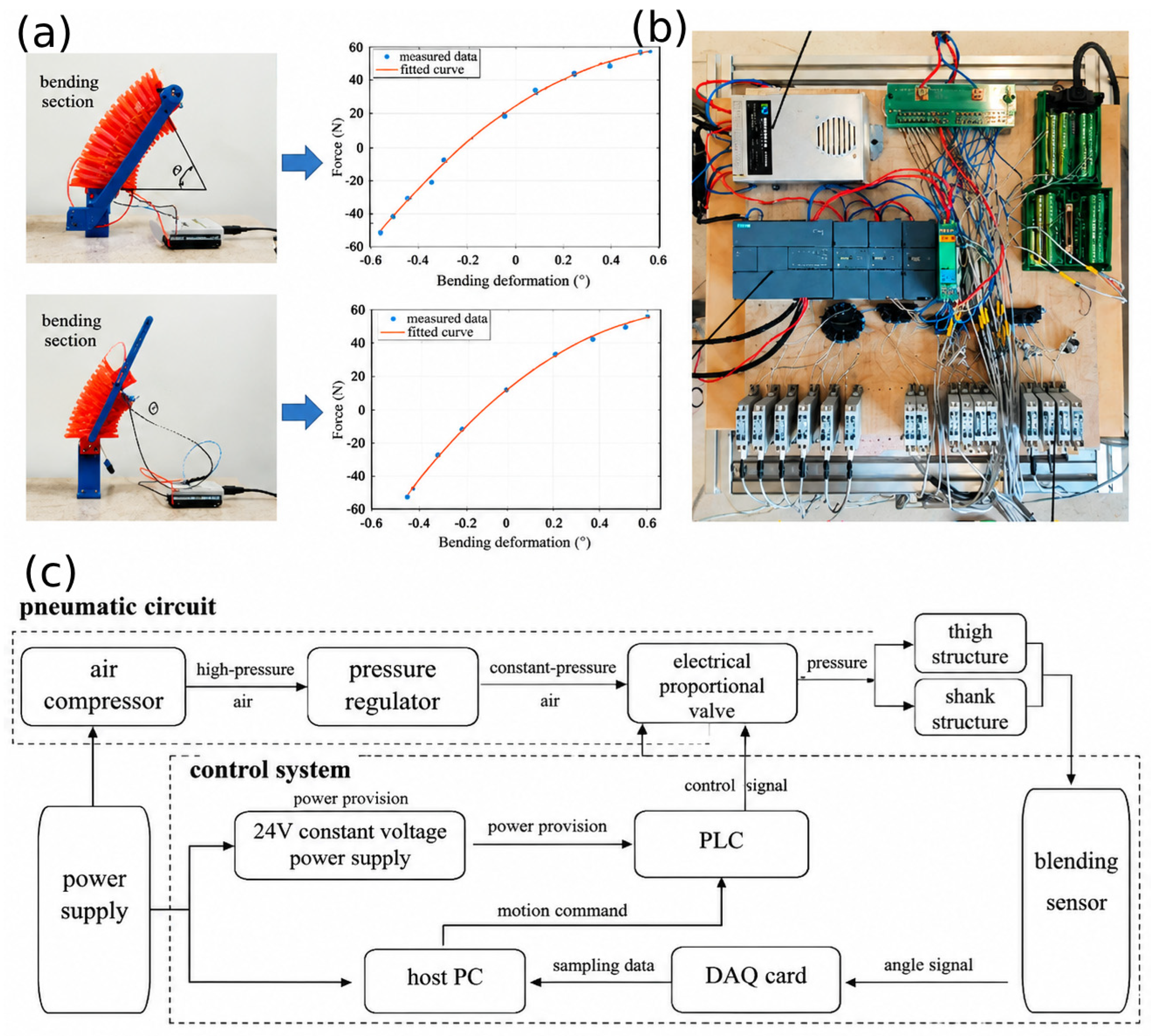
The robot’s four legs are structurally identical, with double-layered honeycomb thighs and single-layered shanks to enable forward movement. The torso has an I-beam shape, which connects several legs and ensures overall stability. During the movement of a single leg, each thigh’s soft actuator is equipped with four independent air channels: two on the inner side and two on the outer side. Each shank, on the other hand, has two air channels. The robot’s control system, shown in Figure 5b, uses an air compressor as the air source, with its pressure regulated by a pressure-reducing valve to feed the proportional valve. The constant-voltage power supply provides power to both the proportional valve and the programmable logic controller (PLC). The detailed control flowchart is shown in Figure 5c. The computer sends action commands to the PLC, which adjusts the input signal of the proportional valve. This controls the air pressure inside the pneumatic honeycomb muscle, thereby changing its degree of bending. This data is simultaneously measured by a bending sensor and collected by the data acquisition card and is then transmitted to the computer for the next step in walking control decisions, creating a closed-loop control system. To determine the bending degree of the soft actuator from sensor voltage data, the bending sensor needs to be calibrated. By adjusting the air pressure within the actuator chamber, different bending degrees are achieved, and the sensor voltage values and the angle between the two ends of the pneumatic honeycomb muscle structure are recorded. Multiple data collections are performed at each signal point to minimize random errors. All data is processed and calculated, with a quadratic polynomial used for fitting, ultimately yielding the calibration curve shown in Figure 5a.

Figure 5. Designed platform. (a) Calibration for bending sensor of the thigh and shank; (b) control system platform; (c) control system flowchart.

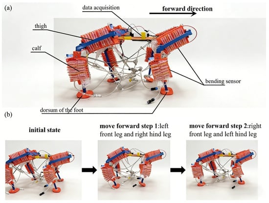
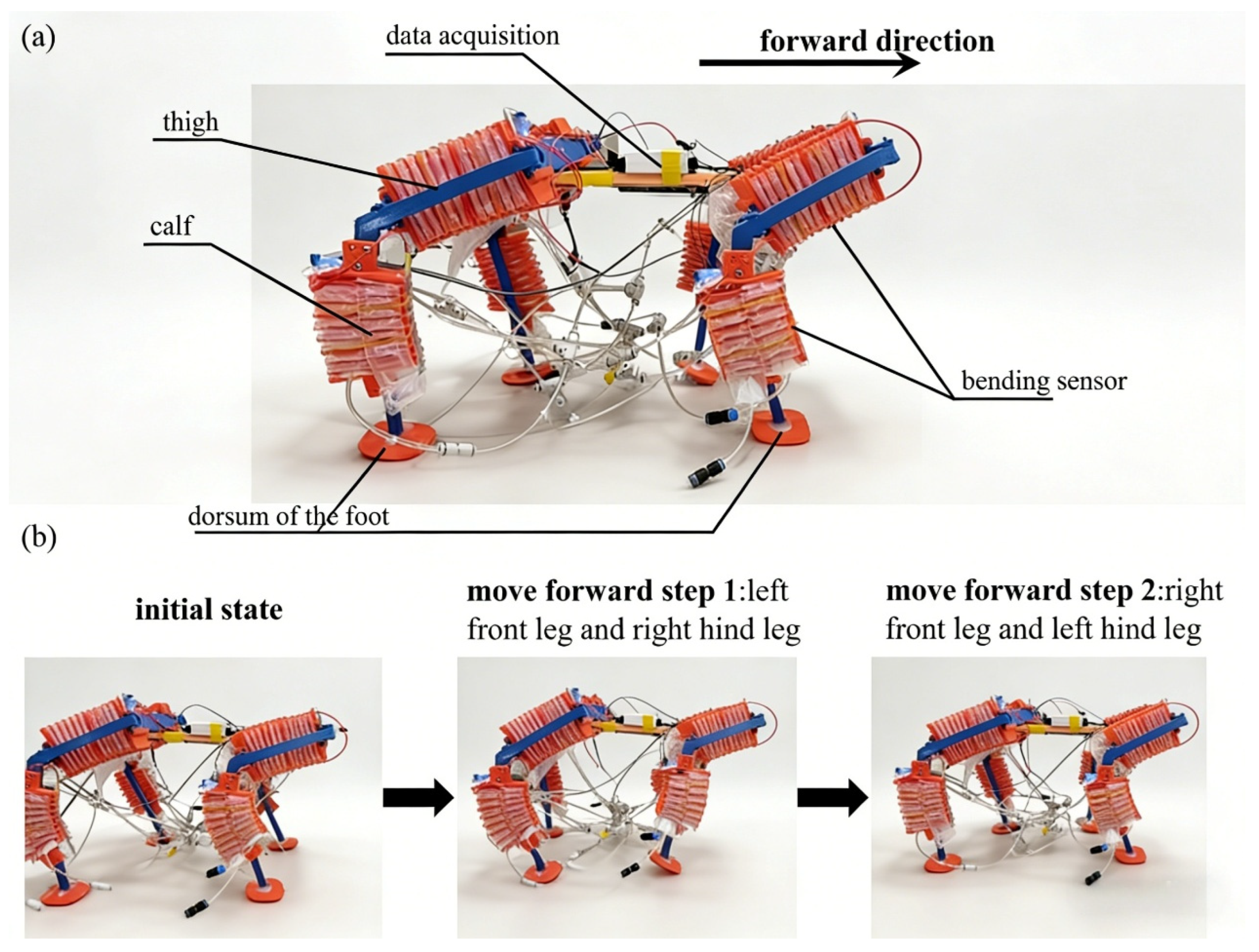
According to the gait plan, the left front leg and right hind leg move forward simultaneously, followed by the right front leg and left hind leg, completing the dynamic walking sequence. The specific walking state of the designed soft quadruped robot is illustrated in Figure 6. At each step, one diagonal leg pair is actuated: the left-front and right-hind legs move first, followed by the right-front and left-hind legs. For a lifted (swing) leg, the outer-side chambers of the double-layer thigh honeycomb actuator are inflated to swing the thigh forward, while the corresponding chamber of the single-layer shank actuator is inflated to bend the shank; the inner-side chambers are inflated for the reverse (return) motion. The other diagonal pair remains inflated and in contact with the ground to support the body.

Figure 6. Designed robot for gait walking. (a) The structure of the soft quadruped robot; (b) the state of moving forward.

4.2. Simulation

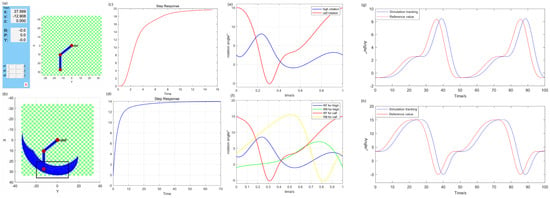
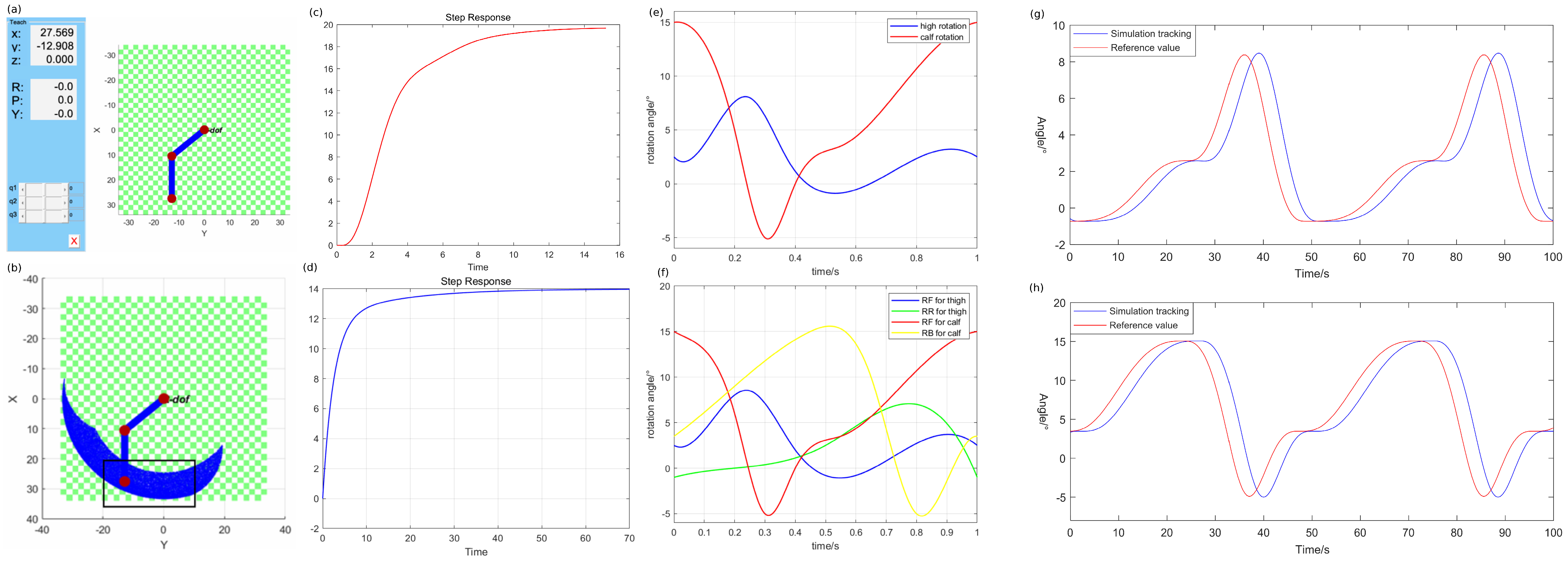
The robot’s structure, algorithm, and actuator model were first analyzed through simulation. In part 3, a simplified D-H model for the robot’s single leg was derived, with l1 = 166.83 mm, l2 = 170.00 mm, and the initial angles of the thigh and shank being β1 = −50.69° and β2 = 50.69°, respectively. Thus, the single-leg model, as shown in Figure 7a, was established. Then, the Monte Carlo method [27,28] was employed to solve the reachable space of the mechanical leg. A total of 30,000 sets of thigh and shank rotation angle arrays were obtained, and the positions of the mechanical leg’s foot end were calculated via forward kinematics. These positions were then visualized using a point cloud diagram, as shown in Figure 7b. In the point cloud diagram, the blue area indicates the reachable range of the mechanical leg’s foot end, and the trajectory planning range of the single-leg foot end is constrained within the black box area. The rotational angle variation curve for a single cycle of the single leg, as planned, is shown in Figure 7c. In dynamic walking, the robot’s diagonal legs exhibit identical movement sequences. The right foreleg (RF) and right hind leg (RB) exhibit a time phase difference of T/2 between them. Hence, the rotational angle curve of the robot’s left legs is shown in Figure 7c. The state-space equation is regarded as the input of the control algorithm. By applying a third-order equation fitting to the data collected from the bending sensor, the parameter matrices in Equation (11) were obtained, as shown below.

$$\begin{array}{l}A=\left[\begin{array}{ccc}-0.1931& 0.2043& 0.0656\\ -0.4248& 0.2443& -0.8856\\ 0.685& 3.051& 1.708\end{array}\right]\\ B=\left[\begin{array}{c}0.003157\\ -0.0225\\ -0.1448\end{array}\right]\\ C=\left[\begin{array}{ccc}655& 46.15& 6.292\end{array}\right]\\ D=\left[0\right]\end{array}$$

(15)

Figure 7. Simulation results. (a) Robot single-leg modeling, (b) accessible and planned intervals, (c) single-leg rotation angle curve, (d) right-leg rotation angle curve, (e) thigh rotation angle tracking curve, (f) calf rotation angle tracking curve, (g) thigh MPC tracking effect in simulation, and (h) shank MPC tracking effect in simulation.

The fitting results indicate that the fit accuracy for the third-order state-space equation is 95.19%. This result demonstrates that applying the state-space equation as the control model is both effective and accurate. The step response curves of the control model for the thigh and shank are shown in Figure 7e,f, where the curves converge, indicating that the system of the designed soft robot is controllable. During the testing of the simulation system, the trajectory curve, sampling time, and other parameters were identical to those in the formal experiment. Parameters were finalized using a trial-and-error approach, setting the prediction horizon to 30, the control horizon to 3, the error weight to 0.1, and the output weight to 10. With these parameters, the simulation effects on the thigh and shank are depicted in Figure 7g,h. The results demonstrate that the tracking curve of the controller’s output is smooth and stable, remaining within the set range. The feedback value of the system rapidly tracks the set trajectory, proving that the system model and algorithm are effective. Thus, the designed robot is suitable for physical experimentation.

4.3. Gait Tracking Control

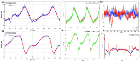
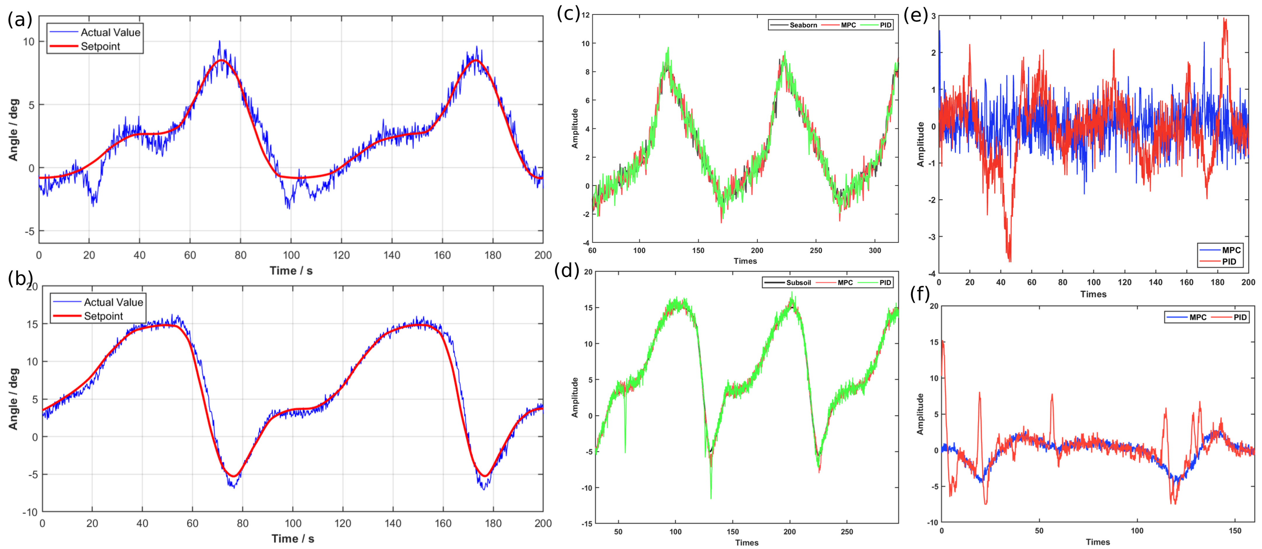
The measured data curves for thigh and shank angle tracking are illustrated in Figure 8a,b. It is evident that the designed robot can quickly and accurately track the set values during its walking process. To verify the performance of the control algorithm, the widely used PID method was compared with the proposed MPC-based control method. Figure 8c,d illustrate the partial tracking trajectories of the two methods for the thigh and shank. It can be observed that the MPC method outperforms the PID method by tracking set values faster, with minimal overshoot and reduced steady-state error. Consequently, the MPC method offers superior real-time adjustment capability. This method can effectively reduce the delay effects introduced by the hardware system, such as the delay in the data acquisition card transmitting the signal from the bending sensor to the computer. It also reduces delays caused by the slow inflation and deflation speed of the soft actuators. This conclusion is also validated by the tracking error graph in Figure 8e,f. As indicated in Table 1, the proposed control method reduced the mean tracking error by 50.98% and 74.92%, and the variance by 7.47% and 71.52%, compared to the PID method. Hence, the accuracy and stability of gait tracking have significantly improved with the proposed MPC-based control method. In the PID comparison, the controller input is the angle error e = r − y (degrees), and the output is the proportional-valve command u (V, limited to +/−3 V); the tuned gains are Kp = 0.06, Ki = 0.02, Kd = 0 for the thigh and Kp = 0.04, Ki = 0.03, Kd = 0 for the shank (the derivative term is negligible for these slow pneumatic processes).

Figure 8. Gait tracking control results. (a) Angle tracking for the thigh based on the MPC method, (b) angle tracking for the shank based on the MPC method, (c) angle tracking comparison for the thigh based on the MPC and PID methods, (d) angle tracking comparison for the shank based on the MPC and PID methods, (e) angle tracking error comparison for the thigh based on the MPC and PID methods, and (f) angle tracking error comparison for the shank based on the MPC and PID methods.

Table 1. Angle tracking error comparison. The reported mean is the mean absolute tracking error (MAE), in degrees, averaged over five repeated trials (n = 5); the variance is the variance of the tracking error, in degrees.

	Mean		Variance
method	thigh	shank	thigh	shank
PID	0.90	0.57	1.28	3.72
MPC	0.44	0.14	1.19	1.06
improvement	51.0%	74.9%	7.5%	71.5%

5. Conclusions

Drawing inspiration from the musculoskeletal movements in nature and incorporating the morphology of quadruped animals, this study proposes the design of a biomimetic quadruped robot. It drives the robot’s limb movements by inflating the pneumatic honeycomb muscle structure to bend. This design effectively combines the strengths of both rigid and soft structures. Based on the designed structure, a soft quadruped air robot was manufactured, and its control system was validated through simulation experiments. Then, physical experiments were conducted on the established control platform. These experiments verified that the control model and algorithm proposed in this paper enable the soft quadruped robot to walk, significantly improving gait tracking accuracy and stability. The results show that the proposed model predictive controller achieved faster and more accurate gait tracking than the conventional PID controller.

References

- Biswal, P.; Mohanty, P.K. Development of quadruped walking robots: A review. Ain Shams Eng. J. 2021, 12, 2017–2031. [Google Scholar] [CrossRef] [Scilit]
- Wang, L.; Wang, C.; Du, W.; Xie, G.; Song, K.; Wang, X.; Zhao, F. Parameter optimization of a four-legged robot to improve motion trajectory accuracy using signal-to-noise ratio theory. Robot. Comput.-Integr. Manuf. 2018, 51, 85–96. [Google Scholar] [CrossRef] [Scilit]
- Kim, Y.; Yuk, H.; Zhao, R.; Chester, S.A.; Zhao, X. Printing ferromagnetic domains for untethered fast-transforming soft materials. Nature 2018, 558, 274–279. [Google Scholar] [CrossRef] [Scilit] [PubMed]
- Lee, C.; Kim, M.; Kim, Y.J.; Hong, N.; Ryu, S.; Kim, H.J.; Kim, S. Soft robot review. Int. J. Control Autom. Syst. 2017, 15, 3–15. [Google Scholar] [CrossRef] [Scilit]
- Pinskier, J.; Howard, D. From Bioinspiration to Computer Generation: Developments in Autonomous Soft Robot Design. Adv. Intell. Syst. 2021, 4, 2100086. [Google Scholar] [CrossRef] [Scilit]
- Beetz, M.; Bartels, G.; Albu-Schaffer, A.; Balint-Benczedi, F.; Belder, R.; Bebler, D.; Haddadin, S.; Maldonado, A.; Mansfeld, N.; Wiedemeyer, T.; et al. Robotic agents capable of natural and safe physical interaction with human co-workers. In Proceedings of the 2015 IEEE/RSJ International Conference on Intelligent Robots and Systems (IROS), Hamburg, Germany, 28 September–2 October 2015; pp. 6528–6535. [Google Scholar]
- Pervez, A.; Ryu, J. Safe physical human robot interaction-past, present and future. J. Mech. Sci. Technol. 2008, 22, 469–483. [Google Scholar] [CrossRef] [Scilit]
- Elango, N.; Faudzi, A.A.M. A review article: Investigations on soft materials for soft robot manipulations. Int. J. Adv. Manuf. Technol. 2015, 80, 1027–1037. [Google Scholar] [CrossRef] [Scilit]
- Fei, Y.; Xu, H. Modeling and Motion Control of a Soft Robot. IEEE Trans. Ind. Electron. 2017, 64, 1737–1742. [Google Scholar] [CrossRef] [Scilit]
- Lei, J.; Yu, H.; Wang, T. Dynamic bending of bionic flexible body driven by pneumatic artificial muscles(PAMs) for spinning gait of quadruped robot. Chin. J. Mech. Eng. 2016, 29, 11–20. [Google Scholar] [CrossRef] [Scilit]
- Tondu, B. Modelling of the McKibben artificial muscle: A review. J. Intell. Mater. Syst. Struct. 2012, 23, 225–253. [Google Scholar] [CrossRef] [Scilit]
- Wu, L.; Chauhan, I.; Tadesse, Y. A Novel Soft Actuator for the Musculoskeletal System. Adv. Mater. Technol. 2018, 3, 1700359. [Google Scholar] [CrossRef] [Scilit]
- Ohta, P.; Valle, L.; King, J.; Low, K.; Yi, J.; Atkeson, C.G.; Park, Y.-L. Design of a Lightweight Soft Robotic Arm Using Pneumatic Artificial Muscles and Inflatable Sleeves. Soft Robot. 2018, 5, 204–215. [Google Scholar] [CrossRef] [Scilit] [PubMed]
- Jing, X.; Jiang, J.; Xie, F.; Zhang, C.; Chen, S.; Yang, L. Continuum manipulator with rigid-flexible coupling structure. IEEE Robot. Autom. Lett. 2017, 2, 11386–11393. [Google Scholar]
- Hongjun, M.; Danyu, R. Design and gait research of pneumatic soft quadruped robot. Adv. Mech. Eng. 2024, 16, 16878132241307827. [Google Scholar] [CrossRef] [Scilit]
- Meng, H.; Zhou, C.; Yang, X.; Zhao, P.; Zhang, W. Design and control of a novel pneumatic soft robot based on the improved particle swarm optimization algorithm. PLoS ONE 2025, 20, e0333187. [Google Scholar] [CrossRef]
- Meng, H.; Zhang, S.; Zhang, W.; Ren, Y. Optimizing actual PID control for walking quadruped soft robots using genetic algorithms. Sci. Rep. 2024, 14, 25946. [Google Scholar] [CrossRef] [Scilit] [PubMed]
- Meng, H.; Zhang, S.; Zhang, W.; Ren, Y. Design and Control of a New Pneumatic Quadruped Soft Robot Based on Honeycomb Structure. IEEE Access 2024, 12, 98882–98899. [Google Scholar] [CrossRef] [Scilit]
- Li, M.; Pal, A.; Aghakhani, A.; Pena-Francesch, A.; Sitti, M. Soft actuators for real-world applications. Nat. Rev. Mater. 2022, 7, 235–249. [Google Scholar] [CrossRef] [Scilit] [PubMed]
- Chen, Y.; Yang, J.; Zhang, X.; Feng, Y.; Zeng, H.; Wang, L.; Feng, W. Light-driven bimorph soft actuators: Design, fabrication, and properties. Mater. Horiz. 2021, 8, 728–757. [Google Scholar] [CrossRef] [Scilit] [PubMed]
- Hainsworth, T.; Smith, L.; Alexander, S.; MacCurdy, R. A Fabrication Free, 3D Printed, Multi-Material, Self-Sensing Soft Actuator. IEEE Robot. Autom. Lett. 2020, 5, 4118–4125. [Google Scholar] [CrossRef] [Scilit]
- Xing, H.; Xu, Y.; Chen, J.; Li, W.; Liu, Y.; Xie, Y.; Ding, L. Multi-objective optimization with priority-based execution for mobile manipulators: An HQP approach integrating adaptive motion planning and obstacle avoidance. Robot. Auton. Syst. 2026, 201, 105457. [Google Scholar] [CrossRef] [Scilit]
- Hu, L.L.; Yu, T.X. Dynamic crushing strength of hexagonal honeycombs. Int. J. Impact Eng. 2010, 37, 467–474. [Google Scholar] [CrossRef] [Scilit]
- Craig, J.J. Introduction to Robotics: Mechanics and Control, 3rd ed.; Pearson Prentice Hall: Upper Saddle River, NJ, USA, 2005. [Google Scholar]
- Jichkar, C.D.; Sondkar, S.Y. Comparative Study of Real Time Implementation of LabVIEW Based MPC Controller and PID Controller for Flow Control Loop. In Proceedings of the 2017 2nd International Conference for Convergence in Technology (I2CT), Mumbai, India, 7–9 April 2017; pp. 464–470. [Google Scholar] [CrossRef] [Scilit]
- Suryawanshi, P.S.; Jadhav, S.P.; Patil, M.D.; Sarode, M.M. LabVIEW Based MPC for Level Control of a Laboratory Setup. In Proceedings of the 2015 International Conference on Communication, Information & Computing Technology (ICCICT), Mumbai, India, 15–17 January 2015; pp. 1–6. [Google Scholar] [CrossRef] [Scilit]
- Kroese, D.P.; Brereton, T.; Taimre, T.; Botev, Z.I. Why the Monte Carlo method is so important today. WIREs Comput. Stat. 2014, 6, 386–392. [Google Scholar] [CrossRef] [Scilit]
- Ferson, S. What Monte Carlo methods cannot do. Hum. Ecol. Risk Assess. Int. J. 1996, 2, 990–1007. [Google Scholar] [CrossRef] [Scilit]
Disclaimer/Publisher’s Note: The statements, opinions and data contained in all publications are solely those of the individual author(s) and contributor(s) and not of MDPI and/or the editor(s). MDPI and/or the editor(s) disclaim responsibility for any injury to people or property resulting from any ideas, methods, instructions or products referred to in the content. |
© 2026 by the authors. Licensee MDPI, Basel, Switzerland. This article is an open access article distributed under the terms and conditions of the Creative Commons Attribution (CC BY) license.