Multi-Objective Optimization of Green Construction Using an Engineering-Oriented Genetic Algorithm: Coordinated Trade-Offs Among Duration, Cost, and Carbon Emissions

Abstract

To address insufficient carbon integration, weakly verifiable quality constraints, and unstable Pareto-set generation in construction-stage green decision-making, this study develops a multi-objective optimization model for construction mode configuration and an engineering-oriented genetic algorithm (GA) framework for Pareto solution generation under hard feasibility constraints. In a construction organization scenario, duration, cost, and carbon emissions are formulated as parallel objectives, while a quality threshold, explicit process logic, and basic resource and workface-feasibility conditions are incorporated to ensure engineering implementability. Construction-stage carbon emissions are quantified using the emission factor method under an auditable activity-level accounting framework. The configured GA framework is compared with the conventional GA, the Non-dominated Sorting Genetic Algorithm II, and the Non-dominated Sorting Genetic Algorithm III through repeated-run statistics and multi-metric evaluation. On the main case, it achieves the highest mean hypervolume (0.723 ± 0.074, mean ± standard deviation), the lowest mean spacing (0.076 ± 0.207), and the smallest average convergence generation (18.49 ± 2.57). The Pareto results reveal a clear trade-off among duration, cost, and carbon emissions, in which high-load beam-and-slab formwork and concrete-related activities dominate cost and carbon variation, whereas schedule advantage mainly depends on stronger compression of critical-chain activities and inter-floor handover.

1. Introduction

1.1. Research Background

The “dual-carbon” targets and the requirements of green construction are reshaping construction management from conventional schedule- or cost-oriented control toward coordinated management of time, cost, and carbon emissions. The construction stage generates substantial emissions through material consumption, equipment operation, and energy use, and thus represents a critical leverage point for decarbonizing the building sector [1]. However, in most engineering practices, construction planning and resource allocation are still dominated by schedule or cost objectives, while carbon emissions are often treated as an ex post accounting and evaluation item rather than being incorporated into plan generation and selection. This leads to a typical “decision disconnect”: a plan may appear optimal in terms of time and cost, yet its embedded energy and emission burdens are not constrained upfront, making it difficult to satisfy low-carbon requirements in green construction. Therefore, it is essential to develop a quantifiable and solvable construction-stage optimization approach that jointly considers time, cost, and carbon emissions and outputs a decision-ready set of candidate solutions within engineering feasibility boundaries, enabling a shift from “accounting-oriented management” to “decision-oriented management”.

1.2. Literature Review

1.2.1. Multi-Objective Optimization

Construction-stage planning was initially formulated largely as single-objective optimization to establish computable decision rules between resource input and organizational choices. Yet single-objective formulations typically embed cost, quality, or environmental impacts as external constraints or after-the-fact checks, which can induce objective bias and increase the risk of infeasible plans. As project decision-making has evolved from “single-metric optimality” to “multi-criteria coordination”, research has progressively moved toward multi-objective frameworks centered on time–cost trade-offs and further incorporated quality and safety dimensions to delineate feasibility boundaries [2,3,4]. Under the dual-carbon agenda, carbon emissions have been increasingly introduced into construction-stage planning, and multi-objective formulations have been extended accordingly [5,6]. Nevertheless, two key gaps remain in engineering applications.

First, feasibility representation is often insufficient. In some studies, quality constraints are still expressed via empirical coefficients, soft constraints, or post hoc filtering, without verifiable thresholds and consistent parameterization, which blurs feasibility boundaries and undermines the “direct implementability” of the resulting solution set. Second, carbon objectives are frequently under-specified. Some studies implicitly proxy carbon emissions by cost and exhibit a tendency of “carbon ex post treatment”, where emissions are primarily used for post-solution comparison or as an auxiliary performance indicator, rather than being introduced as an independent objective alongside time and cost to constrain the search process. From an engineering decision perspective, such an ex post evaluation paradigm may reveal emission differences across plans, but it cannot effectively prevent high-emission solutions from entering the candidate set during optimization, thereby weakening the binding force of low-carbon goals on construction organization decisions. More importantly, carbon emissions and cost are not consistently aligned: depending on material logistics, equipment organization, and energy structure, “low-cost–high-emission” and “high-cost–low-emission” solutions may both be plausible, and using cost as a proxy can distort plan ranking. Consequently, in green construction decision-making, carbon emissions must be introduced upfront as an independent objective parallel to time and cost, so that the optimization outputs a Pareto non-dominated candidate set explicitly reflecting time–cost–carbon trade-offs, which is essential for plan selection under different managerial preferences and carbon constraints.

To address these gaps, this study develops a construction-stage multi-objective optimization model for two-floor construction mode configuration, in which duration, cost, and carbon emissions are treated as parallel objectives under a quality-feasible decision domain.

1.2.2. Genetic Algorithms

Genetic algorithms (GAs) have been widely adopted for construction-stage optimization due to their natural compatibility with discrete combinatorial decisions and relatively low implementation cost; representative studies include GA-based solutions to construction time–cost trade-off problems [7]. However, as optimization expands from single to multiple objectives and constraints shift from weak restrictions to hard feasibility boundaries such as quality thresholds, conventional GAs exhibit structural limitations. First, when search is driven by a single scalarized fitness value, objective bias is likely in multi-objective settings, and it becomes difficult to stably generate a sufficiently diverse and well-covered non-dominated candidate set. Second, in discrete combinatorial spaces, excessive selection pressure can quickly collapse population diversity and induce premature convergence, while insufficient perturbation in later generations weakens continuous boundary exploration, making solution-set coverage and stability highly sensitive to random initialization [8,9].

To better address multi-objective trade-offs and diversity preservation, multi-objective GA frameworks have evolved, among which the Non-dominated Sorting Genetic Algorithm II (NSGA-II) and the Non-dominated Sorting Genetic Algorithm III (NSGA-III) have become mainstream baselines in engineering multi-objective optimization by combining non-dominated sorting with diversity maintenance (e.g., crowding distance or reference points). Their applications in construction have expanded steadily. For instance, improved NSGA-II has been developed for multi-objective resource-constrained project scheduling to enhance computational efficiency [10]. In schedule and parameter optimization scenarios, Building Information Modeling (BIM)-driven multi-objective schedule optimization and shield tunneling parameter optimization have adopted NSGA-III to construct Pareto sets and support decision-making [11,12]. In prefabricated construction, NSGA-II has also been used for construction machinery scheduling and related decisions [13]. Moreover, multi-objective optimization studies in construction management have established a relatively standardized paradigm of “Pareto-front development-preference-based solution selection” in Buildings [14]. While these studies provide reusable algorithmic tools and reporting practices, engineering shortcomings remain when NSGA frameworks are applied to activity–construction mode configuration problems characterized by discrete combinatorics and strongly constrained feasible regions.

Specifically, although NSGA methods are broadly applicable in general multi-objective contexts, hard constraints such as quality thresholds can substantially compress the feasible region and reduce the proportion of feasible solutions. Under such conditions, non-dominated sorting and diversity mechanisms do not necessarily guarantee a sufficient number of feasible non-dominated solutions with balanced distribution; solution-set coverage and boundary exploration can fluctuate with random initialization and selection pressure, weakening the reliability of the candidate set for engineering plan selection. In addition, evidence supporting algorithmic superiority in engineering studies is often “demonstration-oriented”: many works emphasize single-run convergence or illustrative Pareto fronts, yet lack a stability evidence chain based on solution-set metrics, such as hypervolume (HV), and repeated-run statistics, expressed as mean ± standard deviation (SD). In engineering decision-making, if “stable output of high-quality solution sets across repeated runs” cannot be demonstrated, the reusability and interpretability of algorithm outputs may be questioned. These issues indicate that, for construction mode configuration under discrete combinatorics and hard feasibility boundaries, it is necessary to strengthen feasible-solution generation and solution-set updating stability while maintaining the executability of the decision unit, and to establish verifiable evidence through strong baselines and statistical evaluation, so as to meet the practical requirement of reliably producing decision-ready candidate sets.

Building on this rationale, this study develops an engineering-oriented GA framework for construction-stage Pareto solution generation under discrete combinatorics and hard feasibility constraints. The purpose is not to claim a completely new general-purpose evolutionary framework, but to provide a more stable and engineering-oriented solution strategy for quality-feasible green construction planning under explicit process logic.

1.3. Research Work and Contributions

To address the above gaps, this study develops an integrated “model–algorithm–validation” scheme for construction-stage green decision-making.

(1)

A precedence-aware, resource-feasible, and quality-feasible construction-stage optimization model is developed for two-floor construction mode configuration. The model treats duration, cost, and carbon emissions as parallel objectives, while using a hard quality threshold to define the engineering-feasible domain.

(2)

An engineering-oriented GA framework is configured for stable Pareto-solution generation under discrete combinatorics and hard feasibility constraints. The framework integrates feasibility-first updating, elite preservation, stratified probabilistic selection, and dynamic mutation, and its component-wise contribution is further examined through ablation and parameter-robustness analyses.

(3)

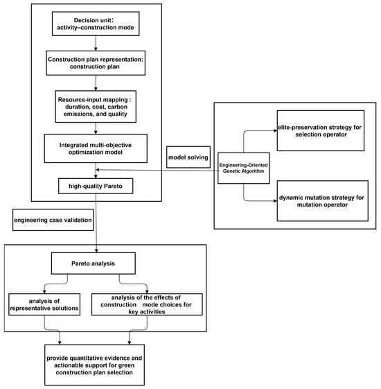
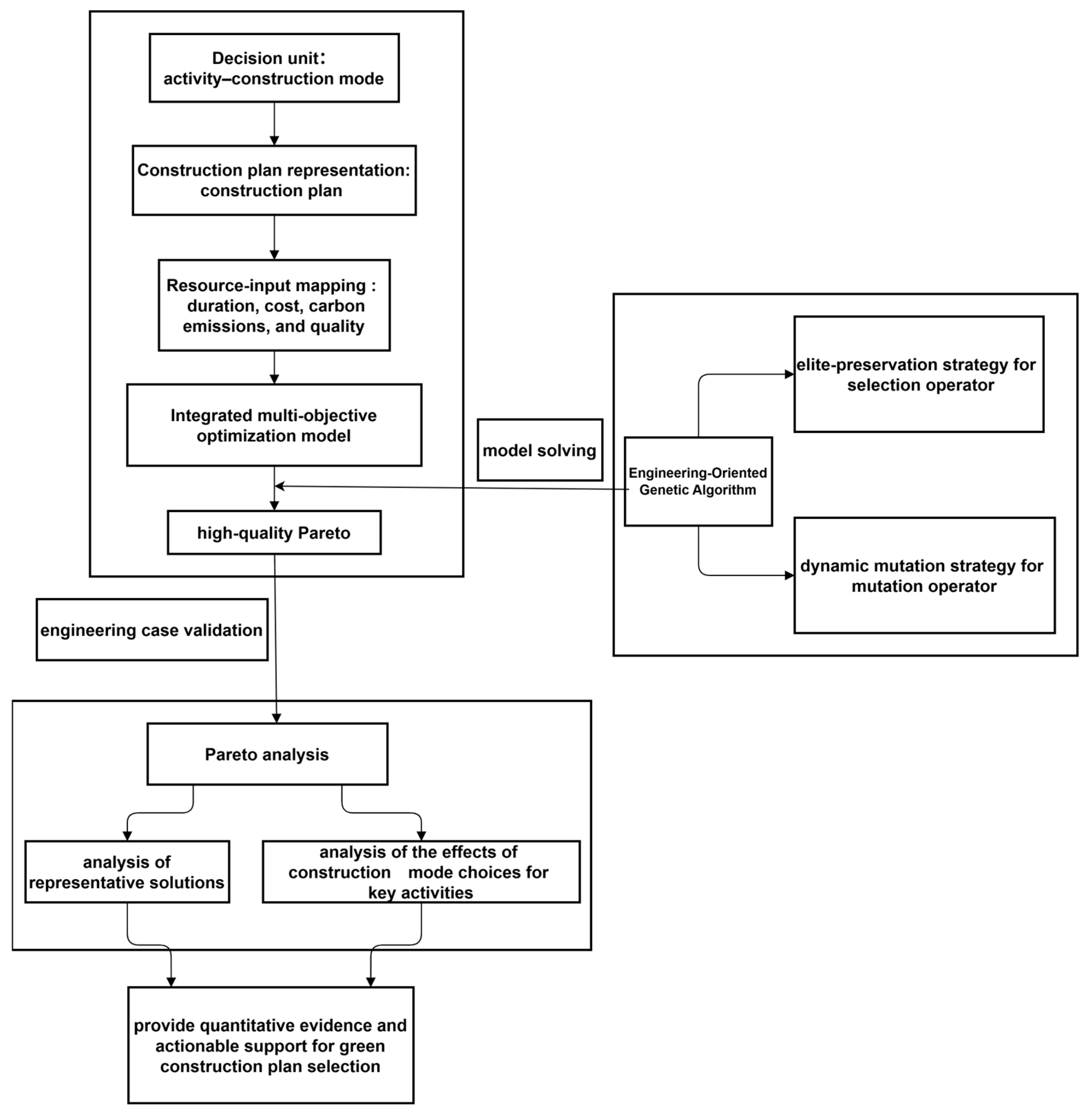
A two-floor construction organization case is used for evidence-based validation. The conventional GA, NSGA-II, NSGA-III, and the configured engineering-oriented GA framework are compared through repeated-run statistics and multi-metric evaluation. The specific research and technical roadmap is shown in Figure 1.

Figure 1. Technical roadmap.

2. Multi-Objective Optimization Model of Time, Cost, and Carbon Emissions

In construction decision-making, differences in resource-input intensity drive the trade-off relationships among duration, cost, carbon emissions, and quality during the construction stage. To quantify these indicators within a unified framework and to enhance engineering interpretability, this study formulates the problem as a construction-stage mode-configuration optimization model for a two-floor construction organization under predefined process logic. Each construction activity is associated with several alternative construction modes, and different modes correspond to different levels of labor, material, and equipment input, thereby leading to measurable differences in activity duration, direct cost, carbon-emission intensity, and quality performance. On this basis, a multi-objective optimization model is established by taking the “activity–construction mode” configuration as the core decision variable and by minimizing duration, cost, and carbon emissions under quality-, process-, resource-, and workface-feasibility conditions.

The present study focuses on a two-floor construction organization scenario, in which process logic can be explicitly defined and activity-level parameters remain auditable. Accordingly, each construction mode-configuration plan is evaluated under a predefined process network with basic labor-, equipment-, and workface-feasibility conditions. Under this scope, the model is intended to support engineering-relevant construction mode configuration rather than to replace comprehensive project scheduling systems.

2.1. Decision Variables

To map differences in resource-input intensity into computable activity-level decisions, the construction organization is assumed to consist of n construction activities (i = 1, 2, …, n), and each activity i is associated with m alternative construction modes (j = 1, 2, …, m). A construction mode represents an executable option for a specific activity. Different modes correspond to different combinations of resource-input levels and organizational strategies, and therefore result in quantifiable differences in activity duration, resource consumption, quality level, and carbon-emission intensity. A binary decision variable X_ij is introduced to describe the selection relationship between activities and construction modes. If activity i adopts construction mode j, then X_ij = 1; otherwise, X_ij = 0. The complete set of X_ij values determines a construction mode-configuration plan and serves as the basis for schedule decoding and for calculating project makespan, total cost, and total carbon emissions under the predefined process-, resource-, and space-feasibility conditions.

For clarity, the main symbols used in the model are summarized here. X_ij denotes the binary decision variable indicating whether activity i adopts construction mode j. S_i and F_i denote the start time and finish time of activity i, respectively, and P denotes the set of precedence relations. T, C, and E denote the total project duration, total cost, and total carbon emissions, respectively. C_ij^dir denotes the direct cost of activity i under mode j, and c^ind denotes the unit-time indirect cost coefficient. E_ij^mat, E_ij^lab, and E_ij^mach denote the material-related, labor-related, and machinery-related carbon emissions of activity i under mode j, respectively. Q denotes the overall construction quality indicator, q_ij denotes the quality coefficient of activity i under mode j, w_i denotes the weight of activity i in the overall quality evaluation, and Q_min denotes the minimum acceptable quality threshold. L_ij and M_ij denote the labor input and key equipment demand of activity i under mode j, whereas L and M denote the corresponding upper bounds for feasible implementation.

2.2. Objective Functions

Within the “activity–construction mode” framework, duration, total cost, and total carbon emissions are evaluated under the predefined two-floor process network. Because different construction modes imply different levels of labor, material, and equipment input, they create unavoidable trade-offs among these three objectives. Project duration is not treated as a simple linear sum of activity durations, but is decoded as the project makespan under precedence relations. Correspondingly, total cost includes both activity-level direct cost and project-duration-related indirect cost. Carbon emissions remain an auditable activity-level objective aggregated over all selected activity–mode combinations.

2.2.1. Duration

When activity i adopts construction mode j, its construction duration is denoted by T_ij. To better reflect engineering organization logic, the total construction duration is defined as the project makespan under a predefined precedence network rather than as a simple sum of activity durations. Let S_i and F_i denote the start time and finish time of activity i, respectively. The finish time of activity i is given by Equation (1):

$$F_i=S_i+{\displaystyle \sum _j{X}_{ij}}{T}_{ij},$$

(1)

where X_ij is the binary decision variable and T_ij is the duration of activity i under mode j.

The precedence requirement between any activity pair (u,v) in the precedence set P is expressed as Equation (2):

$$S_v\ge F_u,\forall (u,v)\in P_v$$

(2)

Accordingly, the total construction duration is defined as the maximum finish time among all activities, as shown in Equation (3):

$$T=\max \left\{F_i\right\},\hspace{1em}i=1,2,\dots ,n$$

(3)

2.2.2. Cost

When activity i adopts construction mode j, the corresponding input structure of labor, materials, and equipment is determined, which in turn defines the direct cost level of that activity. To better reflect the engineering implication of schedule variation, the total construction cost is formulated as the sum of activity-level direct cost and project-duration-related indirect cost, as expressed in Equation (4):

$$C={\displaystyle \sum _i{\displaystyle \sum _j{X}_{ij}}}{C}_{ij}^{dir}+c^{ind}T,$$

(4)

where C denotes the total construction cost; C_ij^dir denotes the direct cost of activity i under construction mode j; cind denotes the unit-time indirect cost coefficient; and T denotes the project makespan obtained under the predefined process logic.

The direct cost of activity i under mode j is decomposed into material, labor, and equipment cost components.

2.2.3. Carbon Emissions

Carbon emissions during the construction stage are quantified using the emission factor method. When activity i adopts construction mode j, its material consumption, labor-service input, and machinery use vary with the selected mode, thereby leading to different emission levels. The total carbon emissions of the construction stage are calculated by aggregating the emissions of all selected activity–mode combinations, as expressed in Equation (5):

$$E={\displaystyle \sum _{i=1}^n{\displaystyle \sum _{j=1}^m{X}_{ij}}}\left(E_{ij}^{mat}+E_{ij}^{lab}+E_{ij}^{mach}\right),$$

(5)

where E denotes the total carbon emissions of the construction stage; X_ij is the binary decision variable; and E_ij^mat, E_ij^lab, and E_ij^mach denote the material-related, labor-related, and machinery-related carbon emissions of activity i under mode j, respectively.

In the two-floor construction organization case, carbon emissions are aggregated over all selected activity–mode combinations in the predefined multi-floor process network. The material-related emissions are calculated as Equation (6):

$$E_{ij}^{mat}={\displaystyle \sum _{k=1}^{K_{ij}}{m}_{ijk}}{e}_k^{mat},$$

(6)

where m_ijk denotes the quantity of material type k consumed by activity i under mode j, and e_fk^mat denotes the corresponding material-emission factor.

The machinery-related emissions are calculated as Equation (7):

$$E_{ij}^{mach}={\displaystyle \sum _{s=1}^{S_{ij}}(f_{ijs}{e}_f^{fuel}+e{c}_{ijs}{e}_f^{ele})},$$

(7)

where f_ijs denotes the fuel consumption of equipment type s, ec_ijs denotes the electricity consumption of equipment type s, efsfuel denotes the fuel-emission factor, and efele denotes the electricity-emission factor.

The labor-related emissions are calculated as Equation (8):

$$E_{ij}^{lab}={\displaystyle \sum _{w=1}^{W_{ij}}{p}_{ijw}}e{f}_w^{lab},$$

(8)

where p_ijw denotes the labor input of labor type w for activity i under mode j, and efwlab denotes the corresponding labor-related emission factor used in this study as a proxy for labor-associated on-site auxiliary resource consumption.

Under this formulation, carbon emissions remain an activity-level auditable objective directly linked to construction mode selection and can therefore be optimized in parallel with duration and cost.

2.3. Constraints

To ensure engineering feasibility, the feasible region is defined through four types of constraints: quality-feasibility constraints, mode-selection consistency constraints, process-logic constraints, and basic resource/workface-feasibility constraints. Specifically, the overall construction quality indicator is defined as the weighted aggregation of the quality performance of each activity under the selected construction mode, as shown in Equation (9):

$$Q={\displaystyle \sum _{i=1}^n{w}_i}{\displaystyle \sum _{j=1}^m{X}_{ij}}{q}_{ij},$$

(9)

where q_ij denotes the quality coefficient of activity i under construction mode j, and w_i denotes the weight of activity i in the overall construction quality, where w_i > 0 and ∑w_i = 1. A minimum quality threshold Q_min is specified, and the corresponding constraint is expressed as Q ≥ Q_min. If a construction plan yields Q < Q_min, it is treated as an infeasible solution and removed during the optimization process. In the present study, the activity weights w_i are assigned according to the relative importance of each activity to overall construction quality, with higher weights given to activities that more directly affect structural integrity, dimensional accuracy, concrete performance, and subsequent acceptance quality.

To improve verifiability and maintain consistency with engineering practice, the quality coefficients q_ij are not assigned as arbitrary empirical scores, but are determined according to current construction quality acceptance specifications [15] and key process-control requirements, including requirements related to reinforcement installation accuracy, formwork stability and dimensional control, concrete pouring and curing conditions, and related technological procedures. For each activity, the three alternative construction modes are evaluated against the corresponding quality-sensitive requirements, and the resulting quality implications are then converted into normalized quality coefficients. The detailed assignment basis of q_ij and w_i by activity type is reported in Table 1, and the same assignment logic is applied to the corresponding activities on Floor 1 and Floor 2. The assignment of q_ij and w_i was carried out by mapping activity-specific quality-sensitive requirements to the corresponding specification-oriented control priorities, and the resulting values were further checked against the engineering importance of each activity in practical quality acceptance.

Table 1. Assignment basis of quality coefficients and weights by activity type.

Code	Name	Weight	Mode	Quality-Sensitive Requirement	Assignment Rationale	Quality Coefficient
1	reinforce column steel bars	0.15	crash	Reinforcement positioning and anchorage accuracy	Faster execution may reduce checking and adjustment time, slightly increasing installation deviation risk	0.99
			normal		Routine labor input and checking procedure satisfy standard requirements with stable quality control	1.03
			economy		Lower resource intensity prolongs duration but still allows compliant installation and inspection	1.01
2	erect column formwork	0.14	crash	Formwork stability, verticality, and dimensional control	Accelerated assembly may weaken alignment and reinforcement checking, slightly increasing formwork deviation risk	0.97
			normal		Normal organization provides stable erection and inspection conditions	1.03
			economy		Lower resource input remains acceptable but provides less redundancy for quality assurance	1.00
3	erect beam and slab formwork	0.18	crash	Support-system stability, elevation control, and dimensional accuracy	Accelerated operation may reduce control time for support spacing and slab-elevation checking	0.96
			normal		Standard process arrangement provides a stable quality level for formwork erection	1.04
			economy		Lower resource intensity prolongs duration but still satisfies minimum control requirements	1.01
4	pour column concrete	0.17	crash	Pouring continuity, vibration quality, and early curing control	Excessive schedule compression may weaken vibration and curing buffering time	0.95
			normal		Normal mode better supports compliant pouring and curing organization	1.04
			economy		Slower pace does not reduce quality and may slightly improve process controllability	1.02
5	reinforce beam and slab steel bar	0.16	crash	Reinforcement spacing, cover thickness, and node detailing	Faster arrangement may increase the probability of local detailing omission	0.98
			normal		Standard organization provides stable control of spacing and node detailing	1.03
			economy		Reduced input remains compliant but provides less redundancy in inspection efficiency	1.01
6	pour beam and slab concrete	0.20	crash	Pouring continuity, vibration effectiveness, surface quality, and curing	Strong schedule compression may increase risks in vibration uniformity and curing adequacy	0.95
			normal		Normal mode provides a stable and specification-compliant process arrangement	1.05
			economy		Longer duration does not inherently reduce compliance and may slightly improve process buffering	1.02

After normalization, a value of 1.0 represents the minimum specification-compliant quality level required for practical implementation. Therefore, Q_min = 1.0 is not an arbitrary numerical setting, but the feasibility baseline corresponding to the minimum acceptable engineering quality. Under this formulation, all solutions entering the Pareto set satisfy the basic quality requirements for practical implementation, while the optimization process remains focused on the real trade-offs among duration, cost, and carbon emissions within a quality-feasible domain.

In addition, mode-selection consistency must be satisfied. For each activity, exactly one construction mode must be selected.

To reflect actual construction organization, process-logic constraints are introduced through a predefined precedence network. Let P denote the set of intra-floor and inter-floor precedence relations. For any (u,v) ∈ P, activity v cannot start before activity u is completed, as already defined in Equation (2).

Basic resource feasibility is further introduced to avoid construction plans that exceed the available organizational capacity during implementation. Let L_ij and M_ij denote the required labor input and key equipment demand of activity i under mode j, respectively, and let L and M denote the corresponding project-level upper bounds for feasible implementation. At the activity level, the selected mode of each activity must satisfy the basic implementability conditions Σ_j X_ijL_ij ≤ L and Σ_j X_ijM_ij ≤ M. In addition, during schedule decoding, the labor and equipment demands of activities that overlap in time are checked against the same project-level capacity limits. If the simultaneous execution of overlapping activities leads to a violation of the available labor or equipment capacity, the corresponding individual is treated as infeasible and excluded from the feasible candidate set.

Finally, space-conflict avoidance is treated through workface-based non-overlap logic. For activity pairs that cannot be executed simultaneously within the same workface or under the same floor-to-floor construction condition, the corresponding precedence or non-overlap relation is included in the process-logic network.

3. Engineering-Oriented GA Framework for Pareto Solution Generation

Genetic algorithms encode candidate solutions as chromosomes and iteratively update the population through feasibility screening, non-dominated sorting, diversity evaluation, selection, crossover, and mutation until the termination criterion is satisfied. For construction-stage multi-objective optimization, however, conventional GAs often suffer from premature convergence in the early search stage and insufficient search efficiency in later iterations. To address these limitations in the present hard-feasibility and discrete combinatorial problem, this study configures an engineering-oriented GA framework by combining feasibility screening, elite preservation, stratified selection, and dynamic mutation, thereby improving computational stability and enhancing the search capability for the non-dominated solution set.

3.1. Encoding

To match the discrete combinatorial decision structure of the “activity–construction mode” formulation, real-number encoding is adopted to represent individuals. Each chromosome consists of a set of gene positions, and each gene corresponds to one construction activity. The gene value, represented in real-number form, indicates the construction mode selected for that activity, thereby mapping a construction plan into an evolvable encoded individual. Real-number encoding reduces the complexity of encoding and decoding and facilitates effective perturbations by crossover and mutation in a continuous search space, which improves search efficiency and the coverage of the solution space.

3.2. Pareto Ranking and Diversity Evaluation

To preserve Pareto consistency and solution-set diversity, this study does not transform the three objectives into a single scalar score for evolutionary updating. For each individual defined by an “activity–construction mode” configuration, the selected activity modes are first decoded under the predefined two-floor process network and basic feasibility rules to obtain the project duration T, total cost C, and total carbon emissions E. These three objective values are then used directly for non-dominated sorting and crowding-distance-based diversity evaluation. Therefore, the Pareto solution set is generated from the original multi-objective dominance relationship rather than from any weighted or normalized aggregation of the objectives. Objective normalization is used only for performance-metric calculation and cross-algorithm comparison under the same reference-point setting.

3.3. Selection

An elitist environmental selection strategy with lexicographic ordering and tiered sampling is adopted to balance convergence and diversity. First, all feasible parent and offspring individuals are merged and ranked by non-dominated sorting. The individuals on the first front are sorted in descending order of crowding distance and copied into the next generation as elites until either the first front is exhausted or the population capacity is reached. If the first front exceeds the remaining capacity, individuals with larger crowding distance are retained first.

The remaining candidates are then ordered lexicographically by ascending Pareto rank and descending crowding distance, and partitioned into three strata according to cumulative population proportion (top 30%, middle 30%, and bottom 40%). Candidates are sampled from these three strata with acceptance probabilities of 0.8, 0.5, and 0.2, respectively, until the next-generation population is filled. Within each stratum, individuals with smaller rank and larger crowding distance are preferred. These tiered proportions and acceptance probabilities are used here as engineering-oriented selection parameters to differentiate selection pressure across solution-quality strata, so that high-quality individuals can be preferentially retained while excessive early-stage selection pressure is alleviated. Their effectiveness and robustness are further examined through the ablation and parameter-robustness analyses in Section 4.4.3.

Under this strategy, elite preservation mainly supports convergence stability, whereas tiered sampling helps maintain solution-set diversity by preventing the remaining population from being dominated too quickly by a small number of highly similar individuals.

3.4. Crossover

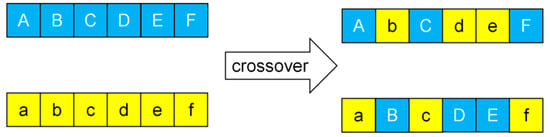
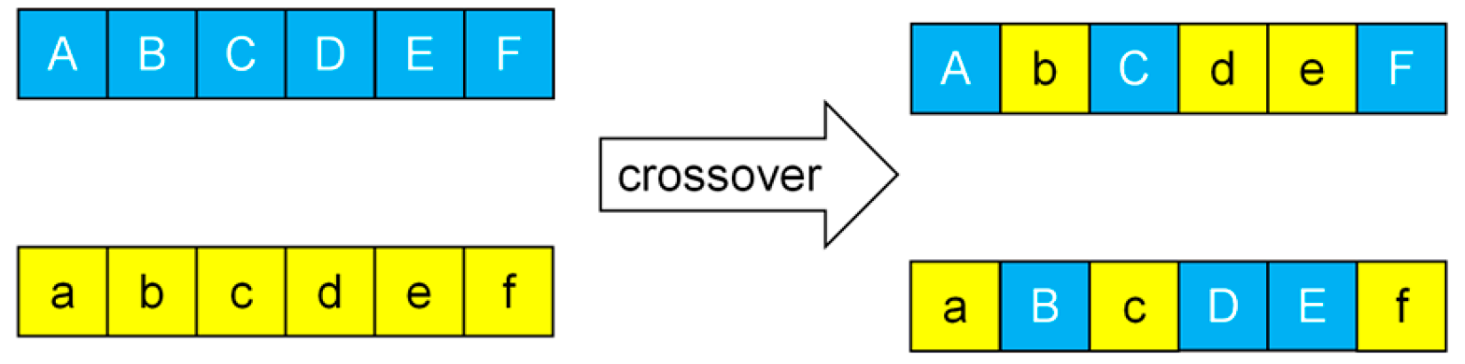
This study adopts a multi-point crossover operator to generate offspring individuals, as shown in Figure 2. In each crossover operation, the number of crossover points is first determined randomly. Corresponding crossover positions are then randomly selected on the parent chromosomes, and gene segments are exchanged at these positions to generate offspring. Multi-point crossover enhances recombination intensity while preserving key gene blocks from the parent individuals, allowing activity–construction mode combinations to be rearranged over a wider range and thereby expanding the search space and improving combinatorial diversity.

Figure 2. Crossover operator. Yellow represents the paternal genes, and blue represents the maternal genes.

3.5. Mutation

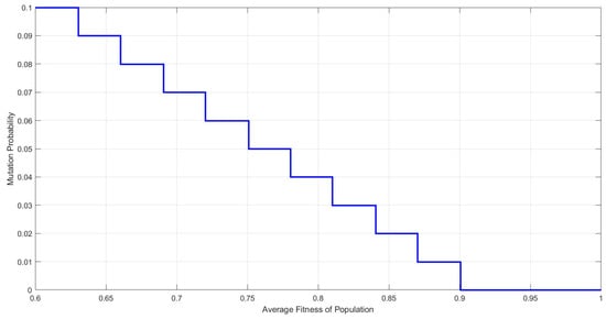
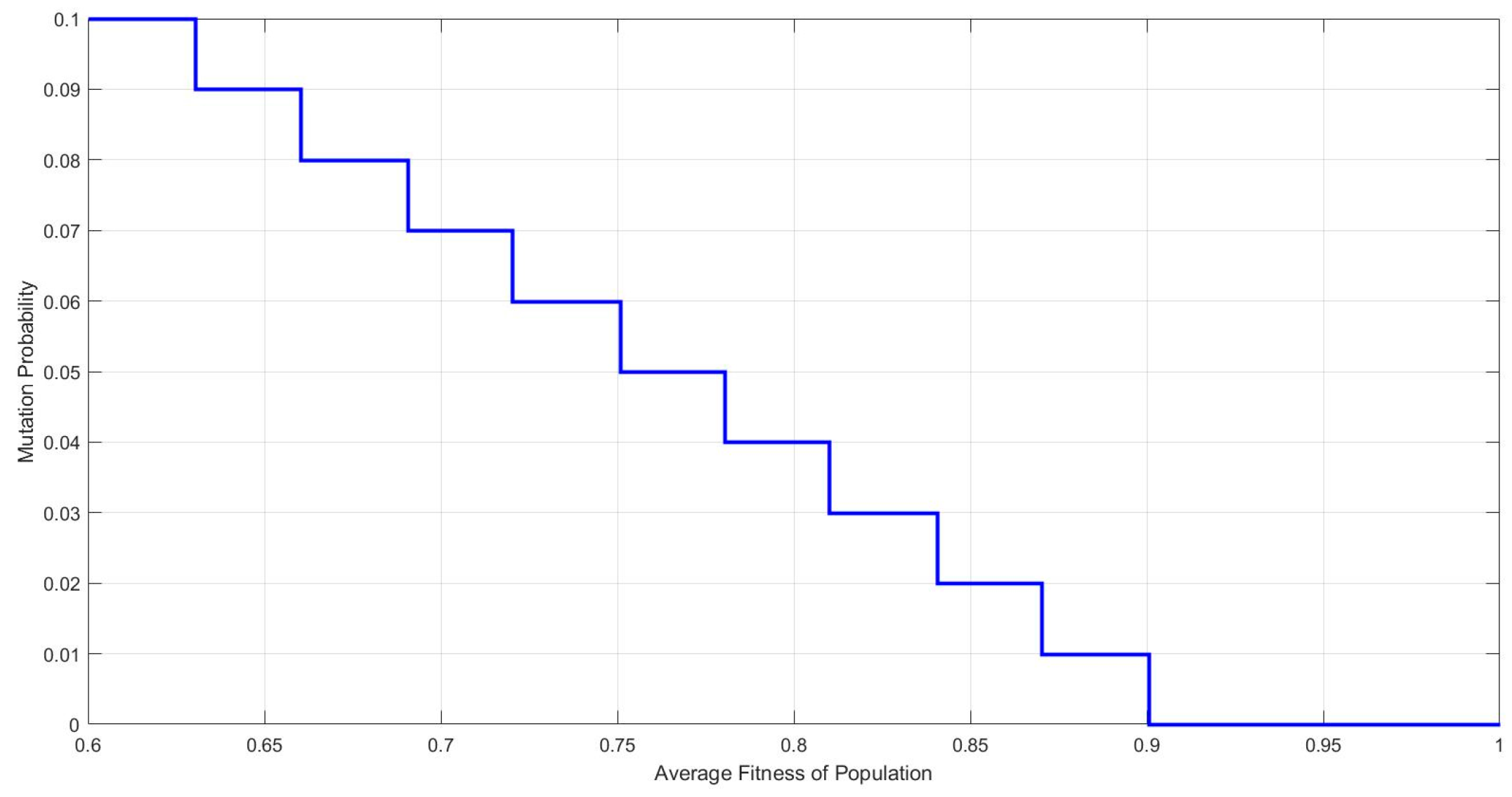
To overcome the limitations of a fixed mutation probability—namely, insufficient exploration in early iterations and excessive perturbation in later iterations—and to reduce the risk of disrupting high-quality individuals, this study improves the mutation operator in two aspects, as shown in Figure 3.

Figure 3. Mutation probability.

First, the mutation probability is adaptively adjusted according to the evolutionary status of the solution set using an HV-driven scheme. Let HV_g denote the hypervolume value at generation g, computed under the same normalization and reference-point setting. If the relative improvement ΔHV_g/HV_{g − 1} remains below 1% for five consecutive generations, the mutation probability is increased by 10% up to the upper bound p_m,max to enhance exploration and facilitate boundary extension of the Pareto set. Conversely, if ΔHV_g/HV_{g − 1} exceeds 3%, the mutation probability is reduced by 10% down to the lower bound p_m,min to promote exploitation and stabilize convergence. These trigger values are used here as practical engineering thresholds for balancing exploration and exploitation.

Second, a Pareto-consistent acceptance criterion is introduced for mutation. After mutation, the offspring is evaluated using the Pareto rank and crowding distance. If the mutated offspring dominates its parent, it is accepted directly. If the offspring and the parent are mutually non-dominated, the one with the smaller Pareto rank is preferred; when they belong to the same front, the one with the larger crowding distance is retained. If the offspring is dominated by the parent, it is retained only with a small probability to preserve exploration capability under hard feasibility constraints. This acceptance mechanism is intended to improve late-stage boundary exploration while avoiding unnecessary disruption of high-quality individuals, and its independent contribution is further examined in the ablation analysis.

Taken together, the dynamic mutation strategy is designed to improve search stability and boundary exploration in the present construction-stage optimization problem.

3.6. Termination Criterion and Multi-Objective Output

The algorithm is terminated when the rank-1 solution set remains stable for five consecutive generations in terms of both set size and boundary solutions, or when the maximum number of function evaluations is reached. After termination, the Pareto solution set in the final population, together with its corresponding objective values for duration, cost, and carbon emissions, is output as the candidate solution set for construction plan selection and trade-off decision-making.

4. Case Study

4.1. Case Background

To verify the engineering applicability of the proposed integrated multi-objective optimization model for construction-stage time, cost, and carbon emissions, as well as the configured model–algorithm framework, a comprehensive frame-structure building project undertaken by a construction enterprise was selected as the case study. Because this type of frame structure typically involves a large number of floors, performing floor-by-floor optimization for the entire building would substantially increase the computational scale and the workload of data preparation. Therefore, this study takes the first floor and a typical floor as the representative research units and formulates the case as a two-floor construction organization scenario with explicit process logic and basic resource/workface feasibility.

4.2. Model Parameter Setting

4.2.1. Construction Activity Decomposition

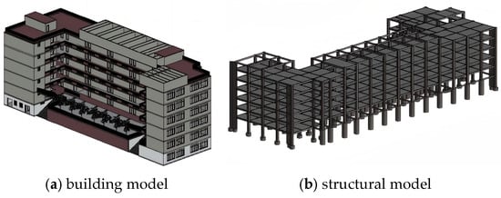
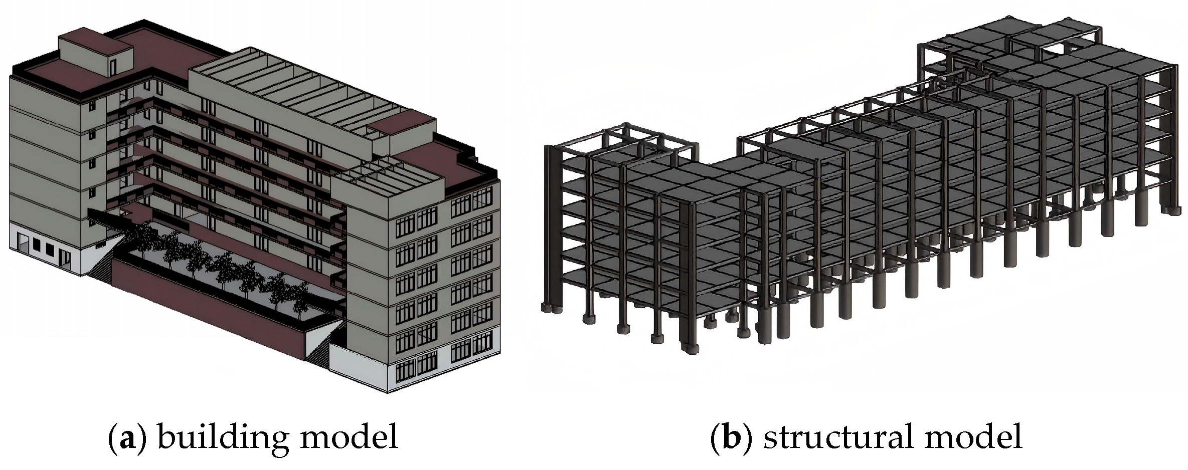
A BIM model of the entire building was established (Figure 4), and the quantities required for construction, including reinforcement, concrete, and formwork, were extracted using quantity takeoff software. Based on the technological sequence and floor-to-floor construction arrangement, the case study is organized as a two-floor, 12-activity construction network.

Figure 4. Three-dimensional model of frame-structure comprehensive building: (a) building model; (b) structural model.

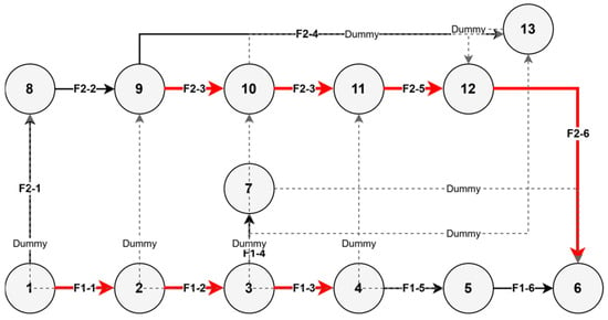
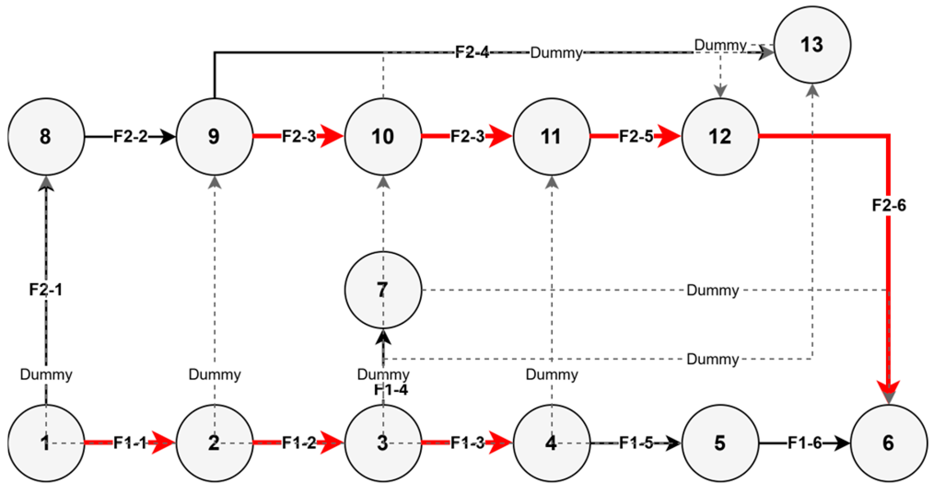
For each floor, the basic activities are defined as follows: column rebar installation, column formwork erection, beam-and-slab formwork erection, column concrete pouring, beam-and-slab rebar installation, and beam-and-slab concrete pouring. Accordingly, the two-floor construction organization consists of Floor 1 activities (F1-1 to F1-6) and Floor 2 activities (F2-1 to F2-6). Within each floor, the activities follow the predefined technological sequence. Across the two floors, additional precedence links are introduced to represent floor-to-floor handover logic, shared-resource occupation, and necessary workface-based non-overlap requirements. Therefore, the evaluation of each construction mode-configuration plan is performed under a basic two-floor process network rather than under a purely serial summation assumption. The predefined precedence network of the two-floor construction organization is illustrated in Figure 5. Specifically, the activities on Floor 2 can start only after the corresponding floor-to-floor handover conditions are satisfied. In addition, selected activity pairs are restricted by shared-resource occupation and workface non-overlap, so that some operations on the two floors cannot be executed simultaneously. Therefore, the two-floor process network includes both technological precedence and organizational feasibility relations.

Figure 5. Predefined precedence network of the two-floor construction organization. Red arrow indicates the critical path, black arrow representes real activity, and dashed arrow denotes dummy activity.

4.2.2. Data Sources and Accounting Basis

The duration and cost parameters are estimated from quantity statistics in combination with local consumption quotas and pricing rules, so that differences in resource input under different construction modes can be translated into quantifiable time and cost values.

Carbon emissions are quantified using the emission factor method. The accounting framework is primarily based on the Standard for Building Carbon Emission Calculation (GB/T 51366-2019) [16], while the underlying activity data are derived from BIM-based quantity takeoff, local quota records, labor-hour records, and equipment shift or energy-consumption records. This combination provides a practical and auditable basis for construction-stage carbon accounting in engineering settings where activity-level resource data are available but process-specific direct emission measurements are difficult to obtain.

In this study, the carbon-accounting boundary is defined as the on-site process emissions associated with construction-stage activity execution under different construction modes. Accordingly, the emission sources are divided into three categories: material-related emissions, labor-related emissions, and machinery-related emissions. Material-related emissions are calculated from material quantities and the corresponding material-emission factors; machinery-related emissions are calculated from fuel and electricity consumption converted from equipment shifts or direct energy-use records; labor-related emissions are calculated from labor input records using corresponding labor-related factors as proxy coefficients for labor-associated on-site auxiliary resource consumption.

To maintain consistency with the decision scope of “activity–construction mode” configuration, the main model focuses on emission items that are directly affected by construction organization and resource-input intensity during on-site execution. Transportation-related emissions are therefore not incorporated into the main optimization objective, because transport distance and upstream logistics are not direct decision variables in the present mode-configuration problem. In addition, the system boundary of material-emission factors follows GB/T 51366-2019, and upstream emissions already reflected in those factors are not repeatedly added during construction-stage accounting. The detailed boundary definition, activity data, and factor basis are summarized in Table 2. For the two-floor construction organization case, the same accounting rules are applied consistently to the activities on both floors, so that the carbon-emission objective remains comparable under the expanded process network.

Table 2. Detailed accounting basis and system boundary for construction-stage carbon emissions.

Accounting Item	Included	Activity Data Basis	Emission Factor Basis	Boundary Treatment	Reason for Inclusion/Exclusion
Material consumption	Included	BIM quantity takeoff and quota-based material consumption	Material-emission factors defined according to GB/T 51366-2019	Included in main model	Directly affected by activity-mode selection
Machinery fuel consumption	Included	Equipment shifts converted into fuel use, or direct fuel records	Fuel-emission factors determined according to GB/T 51366-2019 or corresponding recommended methods	Included in main model	Direct on-site process emission
Machinery electricity consumption	Included	Equipment shifts converted into electricity use, or direct power-use records	Electricity-emission factor determined according to GB/T 51366-2019 or regional adjustment rules	Included in main model	Direct on-site process emission
On-site labor-related activities	Included	Labor-hour records from quota-based activity input	Labor-related proxy factor used in this study	Included in main model	Used to characterize mode-dependent auxiliary on-site resource consumption associated with labor input
Material transportation	Not included in main model	Not directly parameterized in the mode-configuration decision	Not applied in the main model	Excluded from main optimization boundary	Transport distance is not a direct decision variable in the present problem
Material production/processing	Not repeatedly added in construction stage	/	Already reflected in material-emission factors where applicable	Avoided as repeated addition	To maintain consistency with the adopted factor boundary
Equipment manufacturing/depreciation	Not included	/	/	Excluded	Outside the boundary of on-site process emissions
Temporary facilities and ancillary site services	Not included in main model	Not explicitly parameterized	/	Excluded from main optimization boundary	Not directly differentiated across activity-mode choices in this study

Therefore, the carbon-emission parameter of each activity mode is treated as an auditable result derived from quantity statistics, quota-based resource input, and the adopted emission factors under the defined accounting boundary.

4.2.3. Construction Mode Definition and Parameter Representation

To characterize the impacts of resource-input intensity on construction-stage duration, cost, and carbon emissions, three construction modes are defined for each activity: economy, normal, and crash. For the two-floor construction organization case, the activity-level duration, cost, and carbon-emission parameters are reported for all 12 activities, as shown in Table 3. The carbon-emission values reported in Table 3 were calculated according to the accounting boundary and factor basis defined in Section 4.2.2 and then aggregated at the activity-mode level for subsequent optimization. In Table 3, F1 and F2 denote Floor 1 and Floor 2, respectively.

Table 3. Duration, cost, and carbon emissions of each typical-floor activity under different construction modes.

Code	Name	Mode	Duration/Days	Cost/104 CNY	Carbon Emissions/kg
F1-1	reinforce column steel bars	crash	5	4.3	400.67
		normal	6	4.1	356.11
		economy	8	3.8	300.39
F1-2	erect column formwork	crash	8	1.7	339.09
		normal	10	1.5	319.81
		economy	13	1.3	300.81
F1-3	erect beam and slab formwork	crash	18	31.7	5164.15
		normal	23	28.1	4406.49
		economy	28	25.6	3860.53
F1-4	pour column concrete	crash	1	1.7	96.29
		normal	2	1.6	85.15
		economy	3	1.5	68.43
F1-5	reinforce beam and slab steel bar	crash	6	6.4	601.01
		normal	8	6.1	528.59
		economy	10	5.7	450.59
F1-6	pour beam and slab concrete	crash	3	25.6	962.7
		normal	5	24.1	867.93
		economy	8	23.9	806.71
F2-1	reinforce column steel bars	crash	6	5.6	520.87
		normal	7	5.3	462.94
		economy	9	5.0	390.51
F2-2	erect column formwork	crash	9	2.2	470.82
		normal	12	2.0	441.75
		economy	15	1.7	391.05
F2-3	erect beam and slab formwork	crash	21	42	6713.40
		normal	27	37.5	5728.44
		economy	33	34	5018.69
F2-4	pour column concrete	crash	3	2.2	125.18
		normal	4	2.1	110.70
		economy	5	2.0	88.96
F2-5	reinforce beam and slab steel bar	crash	7	8.5	781.31
		normal	10	8.0	687.17
		economy	12	7.5	585.77
F2-6	pour beam and slab concrete	crash	4	34	1251.5
		normal	6	32	1128.31
		economy	10	30	1048.72

To improve the transparency of the quality-feasibility constraint, Table 1 reports the assignment basis of the activity-type-level quality coefficients q_ij and the activity weights w_i. The same assignment logic is applied to the corresponding activities on Floor 1 and Floor 2.

As shown in Table 1, the quality coefficients are activity-specific and mode-sensitive rather than uniformly assigned. This treatment makes the quality-feasibility boundary interpretable in engineering terms and improves the transparency of the optimization model.

4.3. Model Solving and Algorithm Settings

4.3.1. Parameter Settings of the Algorithm

The initial population size is set to 20, the crossover probability is set to 0.7, and the initial mutation probability is set to 0.35. The initial population is generated randomly.

4.3.2. Objective Normalization and Pareto-Based Evaluation Setting

For performance evaluation and cross-algorithm comparison, the objective values were normalized under the same normalization rule and reference-point setting; this normalization did not alter the Pareto dominance relationship during optimization.

4.3.3. Implementation of the Quality Constraint

To avoid infeasible solutions that achieve apparent advantages in duration or cost at the expense of construction quality, a feasibility judgment is embedded into the evolutionary process. During schedule decoding, each candidate individual is checked not only against the quality threshold, but also against the predefined process logic, project-level labor and equipment capacity limits, and workface-based non-overlap requirements. In particular, when two or more activities overlap in time under the decoded schedule, their combined labor and equipment demands are compared with the available project-level capacity. If any precedence violation, resource-capacity violation, or workface conflict is detected, the corresponding individual is classified as infeasible and removed before Pareto ranking. Under this implementation, resource feasibility is evaluated at the decoded schedule level for overlapping activities rather than only at the isolated activity level, so that the model can better reflect basic construction-organization constraints under concurrent execution conditions. The overall quality indicator Q is then calculated according to the corresponding activity–construction mode configuration and compared with the minimum quality threshold Q_min. If Q ≥ Q_min, the individual is regarded as feasible and allowed to enter the population for subsequent evolution; otherwise, it is classified as infeasible and directly removed, without participating in selection, crossover, or mutation.

The quality coefficients q_ij and the activity weights w_i used in feasibility screening are reported in Table 1. After normalization, Q_min = 1.0 represents the minimum specification-compliant quality level required for implementation.

4.4. Comparative Analysis of Algorithm Performance

To evaluate the effectiveness and robustness of the configured engineering-oriented GA framework, comparative experiments were conducted under the same case data, parameter settings, and constraint-handling rules. Four algorithms were considered: the conventional GA, NSGA-II, NSGA-III, and the configured GA framework. The evaluation focused on three aspects: solution-set quality, distribution uniformity, and convergence efficiency. Accordingly, hypervolume, the spacing metric, and convergence generation (G_conv) were adopted as the main indicators, where G_conv denotes the generation at which the rank-1 solution set became stable. During optimization, the Pareto solution set was generated directly from the original objective values of duration, cost, and carbon emissions without scalarization. Objective normalization was used only for metric calculation and cross-algorithm comparison under the same normalization rule and reference-point setting.

4.4.1. Baseline Comparison Under the Main Case

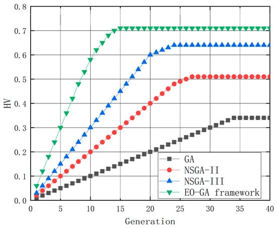
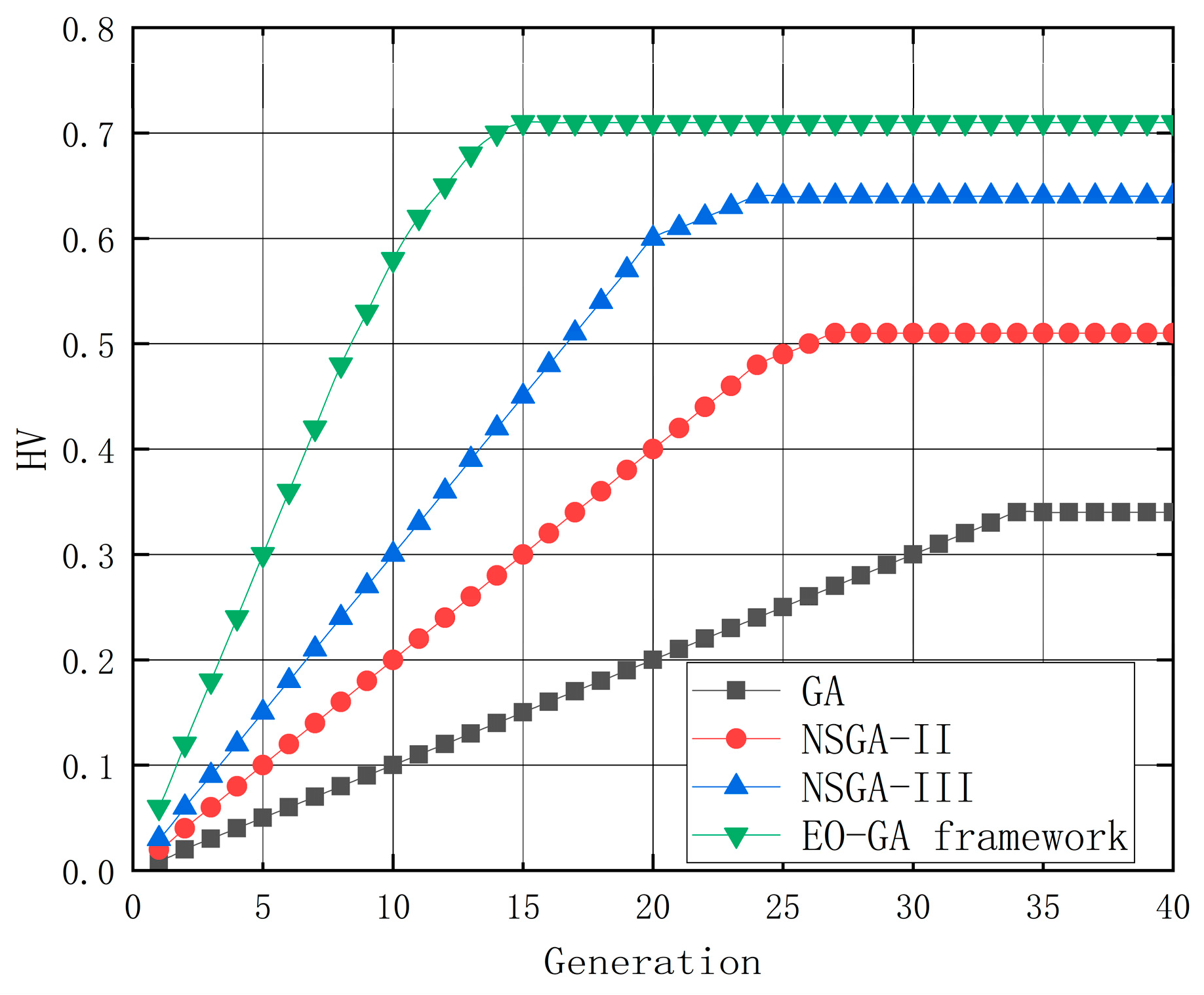
Figure 6 shows the HV convergence curves of the four algorithms under the same function evaluation budget. The configured GA framework exhibits the fastest HV growth and reaches a stable region earlier than the three baseline algorithms, whereas the conventional GA shows the slowest improvement and the largest fluctuation. NSGA-II and NSGA-III both outperform the conventional GA, but remain inferior to the configured GA framework in both convergence behavior and final solution-set quality.

Figure 6. HV convergence curves of GA, NSGA-II, NSGA-III, and the configured engineering-oriented GA framework.

Table 4 reports the repeated-run statistics on the main two-floor construction case. The configured GA framework achieves the best overall performance, with the highest mean HV (0.723 ± 0.074), the lowest mean spacing (0.076 ± 0.207), and the smallest average convergence generation (18.49 ± 2.57). By contrast, the conventional GA shows the weakest performance, with a mean HV of 0.335 ± 0.157, a mean spacing of 0.181 ± 0.341, and an average convergence generation of 35.67 ± 6.74. NSGA-II and NSGA-III both improve the Pareto-set quality relative to the conventional GA. Specifically, NSGA-II reaches 0.507 ± 0.123 in HV and 29.26 ± 4.02 in G_conv, whereas NSGA-III further improves these values to 0.647 ± 0.106 and 24.67 ± 3.15, respectively. However, both remain inferior to the configured GA framework in overall solution-set quality, distribution uniformity, and convergence stability.

Table 4. Repeated-run statistics of GA, NSGA-II, NSGA-III, and configured engineering-oriented GA framework under the main two-floor construction case.

Algorithm	Runs (n)	HV Mean	HV SD	Spacing Mean	Spacing SD	Gconv Mean	Gconv SD
GA	30	0.335	0.157	0.181	0.341	35.67	6.74
NSGA-II	30	0.507	0.123	0.115	0.278	29.26	4.02
NSGA-III	30	0.647	0.106	0.082	0.241	24.67	3.15
EO-GA Framework 1	30	0.723	0.074	0.076	0.207	18.49	2.57

¹ EO-GA Framework denotes the configured engineering-oriented GA framework.

4.4.2. Quality-Threshold Sensitivity

To further examine whether the proposed quality-feasibility setting materially affects the optimization results, a threshold-sensitivity test was conducted using three values, Q_min = 0.98, 1.00, and 1.02, under the same case data, parameter settings, and constraint-handling strategy. For each threshold level, the number of feasible individuals and the characteristics of the representative Pareto plans were compared.

The results show that, as Q_min increases from 0.98 to 1.02, the feasible region becomes narrower, and the proportion of infeasible candidate individuals among all evaluated individuals increases from 10% to 18%. This indicates that a stricter quality threshold compresses the feasible search space and slightly affects solution-set coverage. However, the overall time–cost–carbon trade-off pattern and the ranking logic of the representative schemes remain broadly stable. This suggests that the quality threshold is not merely a formal setting, but an effective engineering-feasibility boundary; at the same time, the main decision conclusions are not fundamentally altered by a moderate tightening of the quality requirement.

4.4.3. Ablation and Parameter-Robustness Analysis

To clarify the contribution of each improvement strategy, an ablation analysis was conducted on the main case. Four variants were compared: the conventional GA, GA with elite preservation only, GA with elite preservation and stratified selection, and the full configured GA framework. As shown in Table 5, elite preservation raises the mean HV from 0.335 to 0.538 and reduces the average convergence generation from 35.67 to 25.43, indicating a clear improvement in convergence stability. After stratified selection is added, the mean HV further increases to 0.664 and the mean spacing decreases from 0.151 to 0.113, showing that this strategy mainly contributes to solution-set distribution and diversity maintenance. The full configured GA framework achieves the best final performance, with the highest HV (0.723), the lowest spacing (0.076), and the smallest G_conv (18.49), which indicates that dynamic mutation further improves late-stage boundary exploration and overall search efficiency.

Table 5. Ablation analysis of the configured engineering-oriented GA framework under the main two-floor construction case.

Algorithm	Runs (n)	HV Mean	HV SD	Spacing Mean	Spacing SD	Gconv Mean	Gconv SD
GA	30	0.335	0.157	0.181	0.341	35.67	6.74
GA + Elite	30	0.538	0.138	0.151	0.287	25.43	3.69
GA + Elite + Stratified	30	0.664	0.096	0.113	0.232	21.69	3.42
EO-GA Framework	30	0.723	0.074	0.076	0.207	18.49	2.57

A lightweight robustness check was also performed for the tiered selection and dynamic mutation parameters. Under three nearby parameter settings, the configured GA framework maintained similar ranking behavior in HV, spacing, and G_conv. The default setting still achieved the best overall balance (HV = 0.723, spacing = 0.076, G_conv = 18.49), whereas the more conservative and more aggressive settings both led to slight reductions in solution-set quality and distribution performance. This result suggests that the adopted parameters function as reasonable engineering settings rather than fragile ad hoc choices.

4.4.4. Cross-Scenario Validation

To reduce the limitation of single-case validation, an auxiliary scenario derived from the same project data was further introduced. Besides the main two-floor case, an additional reduced-scale scenario based on a single-floor activity network was tested. Table 6 shows that the relative performance ranking of the algorithms remains broadly consistent across the two scenarios. In the auxiliary scenario, the configured GA framework still achieves the highest mean HV (0.711 ± 0.024), the lowest mean spacing (0.071 ± 0.229), and the smallest average convergence generation (19.87 ± 1.20). NSGA-III again ranks second, followed by NSGA-II, whereas the conventional GA remains the weakest baseline.

Table 6. Cross-scenario performance comparison of the compared algorithms under the main and auxiliary cases.

Algorithm	Runs (n)	HV Mean	HV SD	Spacing Mean	Spacing SD	Gconv Mean	Gconv SD
GA	30	0.332	0.148	0.174	0.329	34.43	9.07
NSGA-II	30	0.515	0.088	0.109	0.281	27.40	5.12
NSGA-III	30	0.628	0.057	0.075	0.263	24.32	2.76
EO-GA Framework	30	0.711	0.024	0.071	0.229	19.87	1.20

4.5. Analysis of Pareto-Optimal Construction Plans

4.5.1. Trade-Off Characteristics of the Non-Dominated Solution Set

Based on the validated search performance of the configured GA framework, the resulting Pareto-optimal construction plans are further interpreted from the perspectives of overall trade-off structure, representative schemes, and activity-level contribution. The Pareto solution set obtained in this study exhibits a clear trade-off structure among duration, cost, and carbon emissions under the two-floor construction organization scenario. In general, stronger schedule compression is associated with higher cost and larger carbon emissions, whereas lower cost and lower carbon emissions are generally achieved at the expense of a longer construction period. This pattern reflects the basic constraint chain of construction-stage green planning: increasing resource-input intensity can shorten project duration, but it also raises direct construction expenditure and the carbon burden induced by materials, labor, and equipment use.

Rather than forming a few isolated solutions, the non-dominated solution set presents a continuous trade-off band from time-priority to cost-and-carbon-priority. This indicates that the proposed model–algorithm framework can provide a feasible decision spectrum for different managerial preferences instead of a single “best” plan.

4.5.2. Selection and Interpretation of Representative Solutions

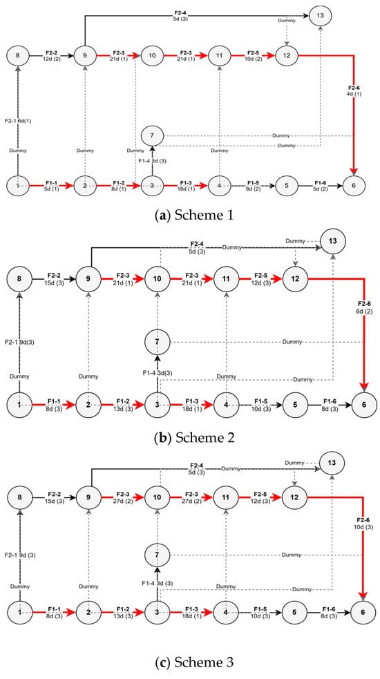
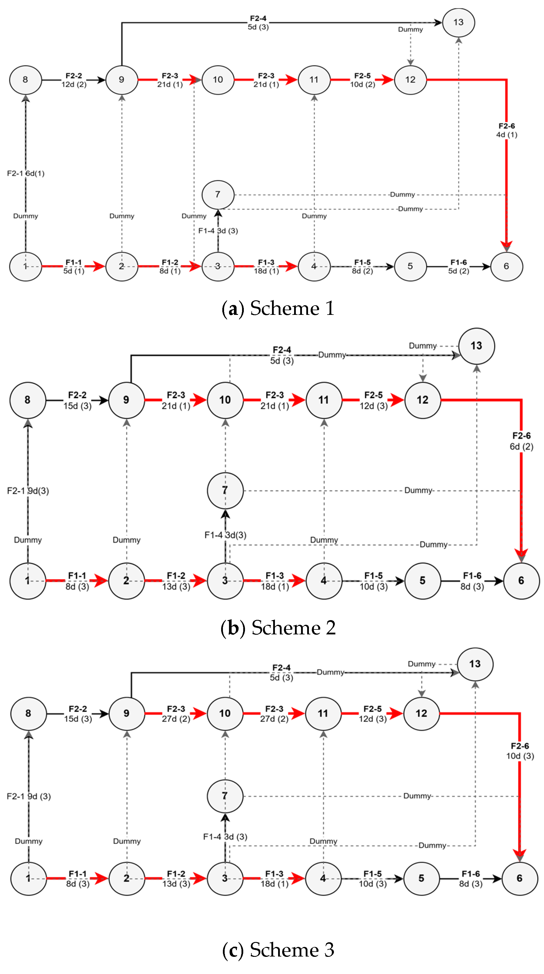
Considering three managerial preference scenarios in practice—schedule priority, balanced coordination, and low-carbon/cost-control orientation—three representative trade-off solutions are selected from the Pareto solution set and presented in Table 7. The corresponding network-plan diagrams are shown in Figure 7, which provide a visual comparison of their activity sequencing and schedule organization under different mode configurations.

Table 7. Pareto solution set and representative construction plans generated under the configured engineering-oriented GA framework.

Scheme	Duration/Days	Cost/104 CNY	Carbon Emissions/kg
1	66	163	17,073
2	78	158	16,389
3	88	155	15,320

Figure 7. Network-plan diagrams of the three representative construction schemes: (a) Scheme 1; (b) Scheme 2; (c) Scheme 3. Red arrow indicates the critical path, black arrow representes real activity, and dashed arrow denotes dummy activity.

The execution-mode coding is defined as follows: crash = 1, normal = 2, and economy = 3.

Scheme 1 achieves the shortest duration (66 days), but also the highest total cost (163 × 10⁴ CNY) and carbon emissions (17,073 kg). This indicates that its schedule advantage is obtained through a more intensive construction organization, especially by strengthening compression on critical-chain activities and inter-floor handover. Scheme 1 is most suitable for projects with rigid milestone requirements.

Scheme 2 represents an intermediate compromise. Compared with Scheme 1, its duration increases to 78 days, whereas total cost and carbon emissions decrease to 158 × 10⁴ CNY and 16,389 kg, respectively. This suggests that moderate schedule relaxation can reduce both economic expenditure and carbon burden without causing excessive delay.

Scheme 3 exhibits the longest duration (88 days), but also the lowest total cost (155 × 10⁴ CNY) and carbon emissions (15,320 kg). Compared with Scheme 1, it reduces total cost by approximately 4.9% and carbon emissions by approximately 10.3%, at the expense of a 33.3% increase in duration. This result indicates that, in the present two-floor construction organization scenario, cost and carbon reduction are mainly achieved by lowering resource-input intensity and reducing schedule compression. Scheme 3 is more suitable when schedule requirements are flexible and low-carbon or cost-control priorities dominate.

4.5.3. Mechanism Interpretation and Activity-Level Contribution Analysis

A deeper examination of the activity-level contributions indicates that the differences among the three representative schemes are mainly driven by a small number of high-load processes rather than by uniform variation across all activities. In all three schemes, F1-3, F2-3, F1-6, and F2-6 jointly account for 80.9–82.0% of total cost and 82.0–84.3% of total carbon emissions. Among them, F2-3 alone contributes 24.7–26.6% of total cost and 37.4–41.0% of total carbon emissions. This result shows that the trade-off structure is dominated by the beam-and-slab formwork and beam-and-slab concrete-related high-load activities on the two floors, rather than by all activities equally.

From the perspective of scheme transition, the mechanism is also clear. Compared with Scheme 2, Scheme 3 reduces total cost by 6.5 × 10⁴ CNY and carbon emissions by 1064.55 kg. Of these reductions, F2-3 alone contributes 69.2% of the cost reduction and 92.5% of the carbon reduction, while F2-6 accounts for most of the remaining change. This indicates that the shift from the balanced scheme to the low-carbon/cost-control scheme is achieved mainly by relaxing compression on the second-floor high-load activities, rather than by uniformly slowing down the entire process network.

By contrast, the transition from Scheme 1 to Scheme 2 is more distributed. The total reduction of 4.9 × 10⁴ CNY and 683.44 kg is jointly contributed by F2-6 and several medium-load activities, including F2-1, F1-1, F2-5, F1-2, F1-5, and F2-2. This suggests that the shift from the schedule-priority scheme to the balanced scheme is realized mainly through a coordinated reduction in resource-input intensity across multiple activities, rather than through the adjustment of a single dominant process.

Overall, the Pareto trade-off is shaped jointly by the unequal resource and energy-intensity structure of different activity types and by their positions in the two-floor construction network. In other words, the differences among the representative schemes arise from how construction intensity is allocated across high-impact and schedule-sensitive activities.

5. Discussion

5.1. Managerial Implications of the Trade-Off

The results indicate that green construction planning should not pursue a single-objective extreme, but should select among multiple quality-feasible compromise plans according to actual managerial priorities. In this sense, the Pareto non-dominated solution set serves as a practical decision interface rather than merely a computational output.

The generalizability of the present findings should be understood appropriately. The validation is based on one engineering case, and the specific Pareto values should not be generalized directly to other projects. However, the case is derived from a typical-floor construction unit in a frame-structure building, and the model is built on generally obtainable engineering information, including activity decomposition, quantity takeoff, quota-based duration and cost estimation, auditable carbon-accounting parameters, and quality-feasibility screening. Therefore, although the numerical results are case-dependent, the underlying “mode configuration–objective evaluation–Pareto selection” workflow is transferable to similar construction-stage planning problems in which activity-level alternatives can be clearly defined and quantified.

5.2. Applicability and Boundary Interpretation

The applicability of the proposed model should be understood within the scope of the adopted two-floor construction organization scenario. The framework is most suitable for construction-stage problems in which decisions can be represented as auditable “activity–construction mode” configurations, activity-level parameters are quantifiable, and a minimum quality threshold must be satisfied. In this study, the model is intended to support mode configuration under a given construction logic rather than to replace full-project scheduling models with complete resource leveling, dense parallel-activity coordination, or refined spatial planning. Accordingly, the main contribution lies more in the modeling logic and decision-support workflow than in the direct transferability of the numerical results.

From the perspective of model validation, the results provide evidence for the broader applicability of the proposed framework to similar construction-stage planning problems. Although the specific Pareto values reported in this study should not be generalized directly, the underlying “mode configuration–objective evaluation–Pareto selection” workflow is transferable when activity-level alternatives, quantifiable inputs, and explicit process logic are available. The present evidence should therefore be interpreted as case-based validation of the workflow rather than as direct proof of universal numerical transferability.

The applicability of the proposed framework may change under different engineering and policy conditions. Carbon pricing, carbon constraints, and low-carbon material substitution may alter the relative attractiveness of alternative schemes by changing both cost ranking and embodied-emission levels. In projects with stronger resource coupling, denser parallel operations, or more severe spatial interference, the representation of process, resource, and workface feasibility may need further refinement.

The carbon results should be interpreted under the adopted site-process-oriented boundary. The additional post-accounting test suggests that a moderate boundary expansion increases absolute carbon values but does not change the ranking of representative schemes, although broader scopes such as material-production variation or wider environmental indicators may still affect the relative attractiveness of alternative plans.

Another important boundary concerns uncertainty. The current model is formulated in a deterministic manner, whereas in practical construction settings, activity duration, labor productivity, equipment availability, energy consumption, and carbon-related parameters may all vary over time. Under such conditions, the position of the Pareto front and the relative ranking of representative solutions may change. Therefore, the present results should be understood as decision support under simplified certainty assumptions. For projects with stronger uncertainty exposure, future extensions toward robust, stochastic, or scenario-based optimization would be more appropriate.

5.3. Limitations and Future Research

Several limitations should be acknowledged. First, the study is still based on a single engineering case, and broader verification across project types, scales, and organizational conditions is still needed despite the inclusion of one auxiliary validation scenario. Second, the carbon-accounting boundary is site-process-oriented. Transportation-related emissions are not included in the main optimization model because transport distance and upstream logistics are not direct decision variables in the present problem, and broader sources such as material-production variation, temporary facilities, and ancillary site services are not explicitly optimized. Third, carbon pricing, policy constraints, and low-carbon material substitution are not currently treated as endogenous decision variables, which means that the present Pareto set should be interpreted under the adopted managerial and accounting assumptions. Fourth, uncertainty is not explicitly modeled; in practical construction environments, duration, labor productivity, equipment performance, and carbon-related parameters may all vary and thereby affect the decision outcome.

Future research can proceed in four directions. The first is external validation across multiple engineering cases to test the stability of the proposed workflow under different project types and organizational scales. The second is boundary expansion, including transportation, broader carbon sources, and low-carbon material alternatives. The third is policy coupling, for example by incorporating carbon pricing, carbon-cap constraints, or other regulatory admissibility rules into the optimization framework. The fourth is uncertainty-aware optimization, such as robust or scenario-based formulations that explicitly account for variability in productivity, cost, and carbon-related parameters. These extensions would improve the forward-looking value of the framework and strengthen its applicability to more complex green construction decision environments.

6. Conclusions

This study develops a multi-objective optimization model for construction mode configuration and an engineering-oriented GA framework for Pareto solution generation. Based on the engineering case, the cross-algorithm comparison, and the trade-off analysis of Pareto-optimal plans, the following conclusions can be drawn.

First, the proposed construction-stage optimization framework enables the coordinated optimization of duration, cost, and carbon emissions while preserving engineering feasibility under the construction organization scenario. Specifically, duration, cost, and carbon emissions are formulated as parallel objectives, whereas construction quality is incorporated as a hard threshold-based feasibility boundary. In addition, the model introduces explicit process logic together with basic resource and workface-feasibility conditions, so that the resulting Pareto solution set remains more consistent with practical construction organization decisions.

Second, the configured engineering-oriented GA framework provides better overall performance than the conventional GA, NSGA-II, and NSGA-III under the same case data, parameter settings, and constraint-handling rules. In the case study, the framework achieves the highest mean HV (0.723 ± 0.074), the lowest mean spacing (0.076 ± 0.207), and the smallest average convergence generation (18.49 ± 2.57), indicating better Pareto-set quality, more uniform distribution, and faster convergence. The ablation results further indicate that elite preservation mainly improves convergence stability, stratified selection mainly enhances solution-set distribution, and dynamic mutation further strengthens late-stage boundary exploration and overall search efficiency.

Third, the engineering case verifies that the proposed model–algorithm combination can stably generate multiple quality-feasible Pareto construction plans and reveal the key trade-off mechanism among duration, cost, and carbon emissions. The results indicate that increasing resource-input intensity generally shortens project duration, but also raises cost and carbon emissions, whereas reducing input intensity improves cost control and carbon mitigation at the expense of a longer construction period. More importantly, high-load beam-and-slab formwork and concrete-related activities dominate the variation in cost and carbon emissions, whereas schedule advantage is mainly associated with stronger compression of critical-chain activities and inter-floor handover.

Overall, the present study provides a practical technical pathway for construction-stage green multi-objective decision-making that balances engineering implementability, solution-set quality, and computational robustness. At the same time, the conclusions should be interpreted within the adopted case and boundary assumptions. Future studies may further strengthen the framework by extending validation across multiple engineering cases, expanding the carbon-accounting boundary, incorporating policy-based conditions such as carbon pricing or carbon caps, introducing low-carbon material alternatives, and developing uncertainty-aware optimization strategies for more complex construction environments.

References

- Yu, J.; Qu, B.; Wei, W. Calculation and Distribution Characteristics of Carbon Emissions during the Construction Phase of Residential Buildings. J. Xi’an Univ. Archit. Technol. (Nat. Sci. Ed.) 2025, 57, 288–296. [Google Scholar]
- Yu, B.; Meng, X.C.; Liu, Q. Multi-objective optimisation of hot in-place recycling of asphalt pavement considering environmental impact, cost and construction quality. Int. J. Pavement Eng. 2020, 21, 1576–1584. [Google Scholar] [CrossRef] [Scilit]
- Panwar, A.; Jha, K.N. Integrating quality and safety in construction scheduling time-cost trade-off model. J. Constr. Eng. Manag. 2021, 147, 04020160. [Google Scholar] [CrossRef] [Scilit]
- Hu, W.; Zhang, Y.; Liu, L.; Zhang, P.; Qin, J.; Nie, B. Study on Multi-Objective Optimization of Construction Project Based on Improved Genetic Algorithm and Particle Swarm Optimization. Processes 2024, 12, 1737. [Google Scholar] [CrossRef] [Scilit]
- Zhang, A.; Zhou, X.; Wang, F.; Yang, J. A multiobjective optimisation and display framework for time–cost–carbon emissions in building materialisation phase based on nD BIM concept. J. Build. Eng. 2025, 103, 111993. [Google Scholar] [CrossRef] [Scilit]
- Wang, H.; Chen, X.; Wang, J. Multiobjective Trade-Off Optimization of Time, Cost, Quality, and Carbon Emission in the Building Construction Stage. J. Constr. Eng. Manag. 2025, 151, 04025009. [Google Scholar] [CrossRef] [Scilit]
- Feng, C.; Liu, L.; Burns, S.A. Using Genetic Algorithms to Solve Construction Time-Cost Trade-Off Problems. J. Comput. Civ. Eng. 1997, 11, 184–189. [Google Scholar] [CrossRef] [Scilit]
- Peng, Z.W. Research on Multi-Objective Optimization of Construction Engineering Based on Improved GA Algorithm. J. Chengdu Technol. Univ. 2022, 25, 55–60. [Google Scholar]
- Zhang, Y.J.; Zhang, B.R.; Wen, G. Multi-Objective Optimization of Green Construction Projects Based on Genetic-Hill Climbing Algorithm. J. Shenyang Jianzhu Univ. (Soc. Sci. Ed.) 2024, 26, 588–594. [Google Scholar]
- Wang, F.; Han, M.C.; Zhao, Y.Y. Multi-Objective Resource-Constrained Project Scheduling Problem Based on an Improved NSGA-II Algorithm. Control. Decis. 2021, 36, 669–676. [Google Scholar]
- Huang, J.T.; Xiao, Z.H.; Zhang, L.M. Research on Multi-Objective Optimization of Super High-Rise Building Construction Schedule Based on BIM and NSGA-III. J. Eng. Manag. 2024, 38, 111–117. [Google Scholar]
- Chen, L.B.; Zhang, M.S.; Chen, H.Y. Analysis and Optimal Control of Shield Tunnel Construction Parameters Based on CatBoost-NSGA-III. Tunn. Constr. (Chin. Engl.) 2024, 44, 1587–1598. [Google Scholar]
- Wang, J.J.; Wang, Z.X.; Liu, H.M. Optimization of Construction Machinery Scheduling Schemes for Prefabricated Buildings Based on NSGA-II. J. Civ. Eng. Manag. 2023, 40, 25–30. [Google Scholar]
- Zhan, Z.; Hu, Y.; Xia, P. Multi-objective optimization in construction project management based on NSGA-III: Pareto front development and decision-making. Buildings 2024, 14, 2112. [Google Scholar] [CrossRef] [Scilit]
- GB 55032-2022; General Code for Construction Quality Control of Buildings and Municipal Engineering. Ministry of Housing and Urban-Rural Development of the People’s Republic of China: Beijing, China, 2023.
- GB/T 51366-2019; Standard for Building Carbon Emission Calculation. Ministry of Housing and Urban-Rural Development of the People’s Republic of China: Beijing, China, 2019.
Disclaimer/Publisher’s Note: The statements, opinions and data contained in all publications are solely those of the individual author(s) and contributor(s) and not of MDPI and/or the editor(s). MDPI and/or the editor(s) disclaim responsibility for any injury to people or property resulting from any ideas, methods, instructions or products referred to in the content. |
© 2026 by the authors. Licensee MDPI, Basel, Switzerland. This article is an open access article distributed under the terms and conditions of the Creative Commons Attribution (CC BY) license.