Two-Stage Damage Identification in Beam Structures Using Residual-Based Wavelet Contrast Index and Improved Dung Beetle Optimizer

Abstract

Accurately identifying damage in beam structures remains a tough challenge, the global trend of wavelet coefficients easily swallows faint local defect signatures, and high-dimensional model updating is computationally inefficient. To tackle these problems, this paper introduces a robust two-stage framework for damage identification that combines a residual-based wavelet strategy with an Improved t-distribution Dung Beetle Optimizer (ITDBO). Rather than relying on guesswork for wavelet selection, we introduce the Residual-based Wavelet Contrast Index (RWCI). By actively stripping away the global trend embedded within the wavelet coefficients, RWCI isolates the pure residual data, drastically amplifying the contrast between genuine stiffness loss and ambient noise for precise damage localization. With the search zone narrowed down, we deploy the ITDBO to quantify the severity. Powered by Bernoulli chaotic mapping and a t-distribution perturbation mechanism, ITDBO effectively bypasses the curse of dimensionality and entirely avoids the premature convergence traps that plague standard metaheuristics. Validated through both numerical simulations and physical experiments on a one-dimensional fixed-fixed steel beam, this hybrid approach proves its mettle. The framework not only accurately flags the defects through heavy noise but also locks onto the exact damage severity with unprecedented efficiency and stability.

1. Introduction

As modern infrastructure continues to age, Structural Health Monitoring (SHM) has become increasingly important for safeguarding bridges, high-rise buildings, and even aerospace structures [1,2,3,4]. In recent years, researchers have gone a step further by developing data-driven decision support systems aimed at improving the safety management of complex systems such as railway bridge networks [5]. As fundamental load-bearing components in civil and mechanical engineering, beam structures are susceptible to the accumulation of early-stage minor damage, which may eventually lead to catastrophic structural failure. Therefore, developing a damage identification method that possesses both high sensitivity and strong robustness is of great engineering significance for assessing the safety status of beam structures. Because of their non-destructive characteristics and ability to provide global structural information, vibration-based damage identification methods have attracted considerable attention in recent years [6,7,8]. Notably, a comprehensive review has further validated the effectiveness of these vibration-based techniques for damage localization and lifetime prediction in bridge structures [9].

In the field of damage localization, signal-processing-based approaches have attracted sustained attention over the past decade. Among them, the Wavelet Transform (WT) has been widely adopted for detecting damage-induced singularities in structural mode shapes, largely because of its strong time–frequency localization capability [10,11]. In practical applications, however, the effectiveness of feature extraction is highly sensitive to the choice of mother wavelet. Different wavelets possess distinct localization characteristics, and this difference can significantly influence how clearly damage signatures are revealed. Traditionally, the selection of a mother wavelet has relied on trial-and-error procedures, Shannon entropy criteria, or similarity metrics between the wavelet basis and the target signal [12,13,14]. While these approaches demonstrate competency in handling simple signals, they frequently falter when applied to intricate modal data. This failure stems from the inherent global curvature of beam mode shapes; this ‘global trend’ generates substantial background coefficients during transformation with certain wavelets, thereby masking the subtle local abrupt changes caused by incipient damage. To make matters more challenging, environmental noise frequently introduces spurious peaks, leading to false positives during localization. Despite ongoing efforts in this direction, there is still a clear lack of an adaptive mother wavelet selection criterion that can effectively suppress modal trend interference while simultaneously enhancing the contrast between genuine damage features and background components. Addressing this gap is therefore both necessary and timely.

Once the damage location has been identified, the next step is to quantify its severity, which is typically accomplished through model updating techniques based on sensitivity analysis or optimization strategies. In this context, evolutionary algorithms have shown considerable promise. For example, Genetic Algorithms (GA) have been successfully integrated into real-time digital twin frameworks for steel bridge monitoring [15]. Recently, meta-heuristic algorithms such as Particle Swarm Optimization (PSO), Grey Wolf Optimizer (GWO), Sine Cosine Algorithm (SSA), and Rime Optimization Algorithm (RIME) have been extensively applied to solve inverse problems in damage identification, owing to their gradient-free nature and ease of implementation [16,17,18,19]. Among emerging swarm intelligence methods, the Dung Beetle Optimizer (DBO) has attracted attention due to its strong global search capability and fast convergence behavior [20]. That said, directly applying optimization algorithms to estimate damage parameters across all structural elements inevitably leads to the so-called “curse of dimensionality.” As the number of variables increases, computational cost grows rapidly, and the risk of getting trapped in local optima becomes more pronounced [21,22]. While DBO holds promise, it remains prone to premature convergence and a loss of population diversity when navigating complex, high-dimensional objective functions characterized by multimodal landscapes. Consequently, establishing a ‘two-stage’ identification framework that synergizes efficient localization with enhanced optimization strategies is pivotal for overcoming these challenges.

Despite the notable progress achieved in structural damage identification, recent two-stage frameworks still exhibit several practical limitations. First, regarding localization, traditional indicators based on modal strain energy or curvature are highly sensitive to measurement noise. They often function as broad-band filters that smooth out the local singularity caused by damage, leading to missed detections in high-noise environments. Second, in the quantification stage, widely used metaheuristic algorithms such as PSO and GWO often struggle with premature convergence. Due to the lack of adaptive mutation mechanisms, these algorithms tend to get trapped in local optima when searching the high-dimensional solution space of inverse problems. This study aims to bridge these specific gaps by introducing a noise-robust wavelet indicator (RWCI) and a structurally enhanced optimizer (ITDBO).

Unlike existing wavelet-based methods that rely on global statistical features (e.g., entropy) and are often compromised when the damage singularity is masked by the global trend of the wavelet coefficients, the proposed RWCI introduces a specialized detrending step. By mathematically removing this trend component from the wavelet coefficients, RWCI isolates the pure residual anomaly induced by damage, offering a significantly higher sensitivity to incipient defects than traditional similarity-based metrics.

Furthermore, in contrast to standard metaheuristic approaches (such as PSO or GWO), which are prone to stagnation in complex multimodal landscapes, the proposed ITDBO integrates Bernoulli chaotic mapping and t-distribution perturbations. These structural enhancements fundamentally alter the search dynamics, ensuring robust global convergence where conventional algorithms typically fail.

To overcome the challenges discussed above, this study develops a two-stage damage identification framework for beam structures by integrating a Residual-Based Wavelet Contrast Index (RWCI) with an Improved t-distribution Dung Beetle Optimizer (ITDBO). The contributions of this work can be summarized from two complementary perspectives.

First, RWCI is proposed to strengthen damage feature extraction during the localization stage. The key idea is to explicitly remove the global trend embedded in the wavelet coefficients through a dedicated de-trending procedure, thereby isolating the pure residual components associated with structural anomalies. On this basis, a contrast index is formulated to quantify the distinction between damage-induced peaks and background noise. In contrast to traditional entropy-based indices, RWCI can adaptively identify the mother wavelet with the highest differentiation margin in noisy environments, enabling precise localization of minor damage.

Second, to address the quantification problem, an enhanced ITDBO algorithm is introduced. Building upon the localization results obtained in the first stage, the parameter search space is significantly reduced, leading to a more tractable reduced-order optimization model. By incorporating Bernoulli chaotic mapping for initialization and a t-distribution perturbation strategy, the standard DBO is refined to bolster its convergence accuracy and robustness. Numerical simulations and experimental validations confirm that this two-stage strategy effectively resolves the issue where modal trends mask damage features, demonstrating superiority over existing methods in both computational efficiency and identification precision.

2. Methods

2.1. Residual-Based Wavelet Contrast Index (RWCI)

To determine the most suitable mother wavelet for damage feature extraction, this study introduces a quantitative evaluation metric grounded in detrended residual saliency. The fundamental basis of this metric is the Continuous Wavelet Transform (CWT). For a given signal f(x)—which corresponds to the modal strain in this study—the wavelet coefficient $W(a,b)$ is calculated as:

$$W(a,b)={\displaystyle \frac{1}{\sqrt{a}}}{\displaystyle {\int }_{-\infty }^{+\infty }f}(x){\psi }^{*}\left({\displaystyle \frac{x-b}{a}}\right)dx$$

(1)

where a is the scale factor, b is the translation factor, and ${\psi }^{*}$ denotes the complex conjugate of the mother wavelet. Because the subsequent damage analysis is carried out at a fixed scale, the scale parameter a remains constant in the following discussion. Under this condition, the translation parameter b directly corresponds to the spatial coordinate x along the structure. In other words, once the scale is specified, shifting the wavelet simply means scanning different spatial locations. For brevity, the wavelet coefficients at a fixed scale are hereinafter denoted as W(x).

Let $\mathbf{\Psi }=\{{\psi }_1,{\psi }_2,\dots ,{\psi }_k\}$ denote the library of candidate wavelet functions. For any given candidate wavelet $\psi \in \Psi$, the computation of its contrast index, $CI(\psi )$, proceeds as follows:

Step 1: Definition of the Effective Analysis Domain

The raw wavelet coefficients W(x) prone to pronounced boundary effects near the signal extremities. These distortions, if not treated properly, can significantly interfere with subsequent damage analysis. To reduce such boundary-induced errors, an effective analysis domain, ${\Omega }_{valid}$, is defined by removing the unreliable data segments at both ends:

$${\Omega }_{valid}=\left\{x\mid x_{start}\le x\le x_{end}\right\}$$

(2)

where $x_{start}$ and $x_{end}$ represent the starting and ending coordinates, respectively, following the truncation of boundary distortions. In this study, based on the observation of the ‘Cone of Influence’ (COI) where boundary errors are significant, the cut-off margin is empirically set to approximately 6–8% of the total span length from each end. For the discretized beam model with 50 nodes, this corresponds to excluding the first and last 3–4 nodes ($x_{start}$ = 4, $x_{end}$ = 47), ensuring the subsequent RWCI calculation is performed on reliable data. All subsequent computations are strictly confined within the range of ${\Omega }_{valid}$, and the truncated wavelet coefficients W(x) are henceforth denoted as $\tilde{W}(x)$.

Step 2: Calculation of Detrended Residuals

The detrended residual is calculated as:

$$R(x)=\tilde{W}(x)-W_{trend}(x)$$

(3)

where $R(x)$ signifies the residual component and $W_{trend}(x)$ represents the global trend component of the wavelet coefficients, which can be derived utilizing the Least Squares Method.

Step 3: Region Partitioning

To assess the prominence of the damage features, the effective analysis domain ${\Omega }_{valid}$ is partitioned into a designated damage region, ${\Omega }_{dmg}$, and a non-damage region, ${\Omega }_{\mathrm{noise}}$. To ensure the damage signature is fully encapsulated while excluding background noise, a peak-centered windowing strategy is adopted. The damage region ${\Omega }_{dmg}$ is defined as follows:

(1) Core Identification: All indices exhibiting significant singularity are identified. Let W(x) be the wavelet coefficient at node x. The set of core indices X_core includes any point where the amplitude exceeds 50% of the global maximum:

$$X_{\mathrm{core}}= \left\{x\mid |R(x)|>0.5\cdot \max (|R|)\right\}$$

(4)

(2) Window Imposition: A window with a width of 10% of the structural span L is imposed around each core index. The damage region ${\Omega }_{dmg}$ is the union of these windows:

$${\Omega }_{dmg}={\displaystyle \underset{x_i\in X_{core}}{\cup }\left[x_i-\frac{0.1L}{2},x_i+\frac{0.1L}{2}\right]}$$

(5)

This formulation ensures that if multiple adjacent points exceed the threshold (e.g., in the case of broad or multi-site damage), the individual windows naturally merge to form a continuous, expanded damage zone.

While the complementary set within ${\Omega }_{valid}$ constitutes ${\Omega }_{\mathrm{noise}}$:

$${\Omega }_{valid}={\Omega }_{dmg}\cup {\Omega }_{\mathrm{noise}},\hspace{1em}{\Omega }_{dmg}\cap {\Omega }_{\mathrm{noise}}=\varnothing$$

(6)

Step 4: Calculation of the Residual-Based Wavelet Contrast Index

$$RWCI(\psi )=\underset{x\in {\Omega }_{dmg}}{\max }|R(x)|-\underset{x\in {\Omega }_{noise}}{\max }|R(x)|$$

(7)

Here, $\underset{x\in {\Omega }_{dmg}}{\max }|R(x)|$ corresponds to the peak signal intensity induced by the damage, whereas $\underset{x\in {\Omega }_{noise}}{\max }|R(x)|$ represents the maximum intensity of background noise or spurious peaks. A higher value of $RWCI(\psi )$ indicates a superior capability of the wavelet to effectively segregate the damage signal from the background noise.

Finally, for the set of candidate wavelet functions, the index value $CI(\psi )$ is calculated for each mother wavelet. The candidate yielding the maximum index is selected as the optimal mother wavelet, ${\psi }_{\mathrm{best}}$:

$${\psi }_{\mathrm{best}}\to \max (RWCI)$$

(8)

Unlike traditional curvature indices where numerical differentiation amplifies high-frequency noise, the proposed RWCI leverages the band-pass filtering property of CWT to isolate singularities. Furthermore, distinct from passive wavelet coefficient methods, RWCI employs an active selection mechanism to maximize the feature-to-noise contrast.

2.2. Improved t-Distribution Dung Beetle Optimizer (ITDBO)

Proposed by Xue and Shen in 2023, the DBO represents a novel addition to the swarm intelligence meta-heuristic family, rapidly garnering significant attention within the computational intelligence community [20]. The algorithm is distinguished not only by its innovative biological underpinnings—mimicking the ball-rolling, dancing, foraging, thieving, and reproductive behaviors of dung beetles—but also its demonstrated effectiveness in solving nonlinear, non-convex, and high-dimensional optimization problems.

Biologically, dung beetles are renowned for their ball-rolling habits. Studies indicate that these insects utilize celestial cues for navigation to maintain a rectilinear trajectory, thereby transporting dung balls to safety via the most efficient path. Furthermore, their social repertoire encompasses oviposition in specific zones to safeguard offspring, the developmental foraging of larvae, and intraspecific theft. These intricate and hierarchical behavioral patterns offer an ideal biological repository for constructing an algorithm equipped with multi-strategy optimization capabilities [20]. Consequently, the mathematical framework of DBO is rigorously mapped to five pivotal natural behaviors: ball-rolling, dancing, breeding, foraging, and stealing.

2.2.1. Bernoulli Chaotic Mapping Initialization Strategy

In the standard DBO framework, the initial positions, denoted as X, are typically generated via pseudo-random numbers:

$$X_{i,j}=l{b}_j+\mathrm{rand}(0,1)\times (u{b}_j-l{b}_j)$$

(9)

where $X_{i,j}$ represents the position of the i-th individual in the j-th dimension, while $u{b}_j$ and $l{b}_j$ define the upper and lower bounds of the search space, respectively. The term $\mathrm{rand}(0,1)$ signifies a random variable following a uniform distribution. However, given the stochastic nature of the rand function, guaranteeing ergodicity within the search space remains challenging, particularly under constraints of limited population size.

To address this limitation, Bernoulli chaotic mapping is introduced to replace the conventional pseudo-random initialization scheme. Unlike purely random sampling, chaotic sequences exhibit properties such as non-repetition, ergodicity, and deterministic pseudo-randomness. These characteristics allow the generated variables to traverse the solution space more thoroughly, resulting in a more uniform and diverse distribution of the initial population. In practical terms, this means that candidate solutions are less likely to cluster in a limited region of the search domain at the outset, thereby improving global exploration from the very first iteration. The iterative mathematical formulation of the Bernoulli map is defined as

$$z_{k+1}=\left\{\begin{array}{ll}{\displaystyle \frac{z_k}{1-\lambda }},\hfill & 0<z_k\le 1-\lambda \hfill \\ {\displaystyle \frac{z_k-(1-\lambda )}{\lambda }},\hfill & 1-\lambda <z_k<1\hfill \end{array}\right.$$

(10)

Typically, the parameter λ is set to 0.5, simplifying the expression to the classic Bernoulli shift map:

$$z_{k+1}=(2z_k)\hspace{1em}\mathrm{mod} 1$$

(11)

where $z_k$ ∈ (0, 1) is the chaotic sequence value at the k-th iteration, and mod1 denotes the fractional part. The initial value z₁ is randomly generated within the interval (0, 1), ensuring that z₁ ≠ 0.5 to avoid fixed-point stagnation. Leveraging the generated chaotic sequence Z = {z₁, z₂, …, z_N}, the population is mapped back into the solution space using the improved initialization equation:

$$X_{i,j}^{\mathrm{new}}=l{b}_j+z_{i,j}\cdot (u{b}_j-l{b}_j)$$

(12)

In contrast to the standard rand function, the ergodicity inherent in the chaotic sequence $z_{i,j}$ ensures a higher probability of exploring both the peripheral and central regions of the search space. This mechanism yields high-quality initial candidate solutions for subsequent iterations, thereby accelerating the algorithm’s convergence rate.

2.2.2. Adaptive t-Distribution Perturbation Mechanism

Within the standard DBO framework, the position update equations—whether for ball-rolling, foraging, or thieving behaviors—invariably incorporate a vector directed towards the current global optimum, X_best. However, a critical vulnerability arises during the latter stages of iteration or when navigating multimodal objective functions: the population tends to cluster. As the term $\left|x_i(t)-X_{best}^g\right|$ approaches zero, the population is stripped of its diversity, often precipitating premature convergence at local optima.

To alleviate this tendency toward stagnation, a mutation strategy based on the t-distribution is incorporated into the algorithm. Rather than being activated only under specific conditions, this mutation mechanism is embedded directly into each iteration as an auxiliary update applied to the global best position. In other words, it operates continuously alongside the standard search process, subtly enhancing diversity without disrupting the overall optimization framework. The rationale behind this design is to introduce controlled perturbations that allow the algorithm to escape potential local optima while preserving convergence stability. Its probability density function, p(x), is defined as follows:

$$p(x)={\displaystyle \frac{\Gamma \left(\frac{n+1}{2}\right)}{\sqrt{n\pi }\Gamma \left(\frac{n}{2}\right)}}{\left(1+{\displaystyle \frac{x^2}{n}}\right)}^{-{\displaystyle \frac{n+1}{2}}}$$

(13)

where n denotes the degrees of freedom and Γ is the Gamma function. The t-distribution exhibits unique characteristics that render it highly suitable for adaptive perturbation: As n → 0, the distribution converges towards a Cauchy distribution, characterized by significant “heavy-tailed” properties. This yields a higher probability of generating large mutation steps, which facilitates global exploration. Conversely, as n → ∞, it approximates a Gaussian distribution, where mutation values concentrate near zero, thereby favoring local exploitation.

In the proposed strategy, the current iteration number t acts as an adaptive parameter to modulate the degrees of freedom. The mutation is applied to the current global best position $X_{\mathrm{best}}(t)$ to generate a new candidate position $X_{\mathrm{new}}(t)$:

$$X_{\mathrm{new}}(t)=X_{\mathrm{best}}(t)+X_{\mathrm{best}}(t)\cdot t(t)$$

(14)

where $\mathrm{t}(t)$ represents a t-distributed random variable with degree of freedom t.

During the early stages of the optimization process, when the degrees of freedom t are relatively small, the mutation operator exhibits behavior similar to a Cauchy distribution. In this regime, the perturbations are heavy-tailed and comparatively large, enabling the algorithm to make bold jumps across the search space. Such high-amplitude variations are particularly effective in dislodging individuals that may have become trapped in local optima.

As the iteration count increases and the degrees of freedom gradually grow, the t-distribution progressively approaches a Gaussian profile. Correspondingly, the mutation step becomes more moderate and concentrated around the current best solution. This shift from large exploratory moves to subtle local refinements allows the algorithm to transition smoothly from global exploration to fine-grained exploitation. In practical terms, it improves the precision of convergence while maintaining overall search stability.

Finally, to avert any degradation in solution quality caused by mutation, a greedy selection mechanism is employed to decide whether to update the optimal position:

$$X_{\mathrm{best}}(t)=\left\{\begin{array}{cc}{X}_{\mathrm{new}}(t),\hfill & f\left(X_{\mathrm{new}}(t)\right)<f\left(X_{\mathrm{best}}(t)\right)\hfill \\ X_{\mathrm{best}}(t),\hfill & \mathrm{otherwise}\hfill \end{array}\right.$$

(15)

where f represents the fitness function.

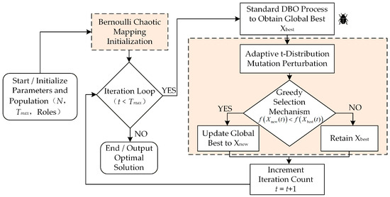
Figure 1 presents the schematic flowchart of the Improved t-distribution Dung Beetle Optimizer (ITDBO). This enhanced framework integrates Bernoulli chaotic initialization with an adaptive t-distribution mutation strategy, finalized via a greedy selection mechanism. The modules enclosed within the dashed frames delineate the specific improvements introduced to the conventional DBO structure.

Figure 1. Schematic flowchart of the ITDBO.

2.3. Definition of Element Damage Severity

In this study, the damage severity is quantified by the degradation of the beam’s flexural rigidity, formulated as:

$$E{I}_S=EI\times (1-\gamma )$$

(16)

where EI and $E{I}_S$ denote the flexural rigidity of the intact (undamaged) and damaged cross-sections, respectively, while γ represents the damage severity index. By leveraging the geometric properties of the rectangular cross-section and the parallel axis theorem, the relationship between stiffness reduction and crack geometry is established as:

$${(h-d)}^3+3d^2(h-d)=h^3(1-\gamma )$$

(17)

where h refers to the height of the beam section, and d signifies the crack depth corresponding to the specific damage severity. Disregarding the non-physical complex roots of Equation (17), the explicit solution for the crack depth is derived as:

$$d={\displaystyle \frac{h}{2}}\left(1-{(1-2\gamma )}^{{\displaystyle \frac{1}{3}}}\right)$$

(18)

Consequently, Equation (18) provides a direct analytical method to convert the theoretical damage severity γ into the physical crack depth d for finite element modeling.

2.4. Objective Function

To accurately quantify damage severity, an objective function is constructed by integrating natural frequencies with mode shapes. This hybrid approach compensates for the insensitivity of frequencies to local defects. The objective function is expressed as the weighted sum of the squared relative errors [18]:

$$\min F=G_{\omega }{\displaystyle \sum _{i=1}^m(}{\displaystyle \frac{f_i^{test}-f_i^{cal}}{f_i^{test}}}{)}^2+G_{\varphi }{\displaystyle \sum _{i=1}^n{\displaystyle \sum _{j=1}^k(}}{\varphi }_{ij}^{test}-{\varphi }_{ij}^{cal}{)}^2$$

(19)

where f_i and ${\varphi }_{ij}^{test}$ denote the natural frequency of the i-th mode and the displacement mode shape component at the j-th node of the i-th mode, respectively. The superscripts ‘test’ and ‘cal’ distinguish between experimental measurements and numerical calculations. The coefficients $G_{\omega }$ and $G_{\varphi }$ weight the contributions of frequency and mode shape errors; both are set to 1.0 in this analysis. Variables m, n, and k correspond to the number of frequency orders, mode shape orders, and sensor locations, respectively. The minimization of F ensures that the updated finite element model optimally matches the physical structure’s dynamic behavior.

During the preparation of this manuscript, the authors used ChatGPT (Model GPT-5.0) for the purposes of translation and English language refinement. The authors have reviewed and edited the output and take full responsibility for the content of this publication.

3. Numerical Simulation

3.1. Selection of the Optimal Mother Wavelet and Damage Localization

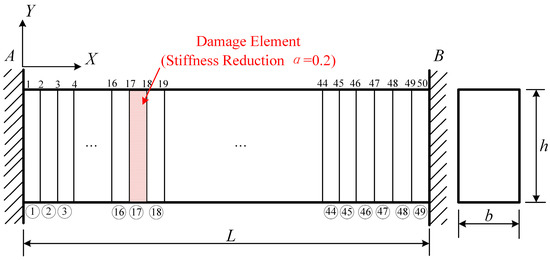
For the numerical setup, we modeled a fixed-fixed Q235 steel beam, as illustrated in Figure 2. The structure spans 1274 mm in length with a 60 mm × 80 mm rectangular cross-section. We assigned standard material properties for the steel: an elastic modulus (E) of 210 GPa, a density (ρ) of 7800 kg/m³, and a Poisson’s ratio (ν) of 0.3.

Figure 2. Schematic diagram of the fixed-fixed beam finite element model.

We built the finite element model (FEM) in ANSYS 2024R1, meshing the structure into 49 uniform BEAM188 elements, each 26 mm long. To set up the damage scenario, we introduced a through-width transverse crack at Element 17—located roughly one-third of the way (1/3L) from the left support—with an equivalent depth of 6.26 mm (γ = 20%).

Once we extracted the displacement mode shapes from the modal analysis, Gaussian white noise at varying signal-to-noise ratios (SNRs) is superimposed to mimic realistic environmental interference. Next, we calculated the curvature and strain modes using a second-order central difference method. For the actual wavelet transform, we relied on MATLAB’s Wavelet Toolbox. We specifically targeted the strain mode data rather than displacement—since strain is far more sensitive to localized stiffness drops—and extracted the corresponding wavelet coefficients to feed into our damage identification process.

In practice, vibration measurements are inevitably susceptible to environmental noise contamination. To test how robust our method is under these real-world conditions, we intentionally added Gaussian white noise to the numerical responses. We control this noise level using the Signal-to-Noise Ratio (SNR), defined as:

$$SNR=20lo{g}_{10}\left({\displaystyle \frac{{\sigma }_s}{{\sigma }_n}}\right)$$

(20)

where ${\sigma }_s$ and ${\sigma }_n$ denote the standard deviations of the effective signal and the added noise, respectively. We opted for Gaussian white noise in these simulations because it serves as an excellent proxy for the broadband thermal and electronic noise you typically encounter in piezoelectric data acquisition setups. The specified SNR levels (90 dB to 60 dB) were chosen to simulate scenarios ranging from ideal laboratory environments to high-interference field conditions. While operational environments may introduce non-Gaussian noise—such as low-frequency drift from wind or harmonic vibrations from machinery—the multi-scale nature of the WT provides inherent filtering capabilities. By localizing features in the scale domain, the proposed RWCI maintains robustness against such interferences, provided that the spectral characteristics of the noise do not coincide with the high-frequency band of the damage singularity.

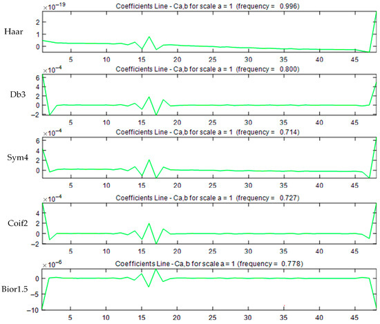
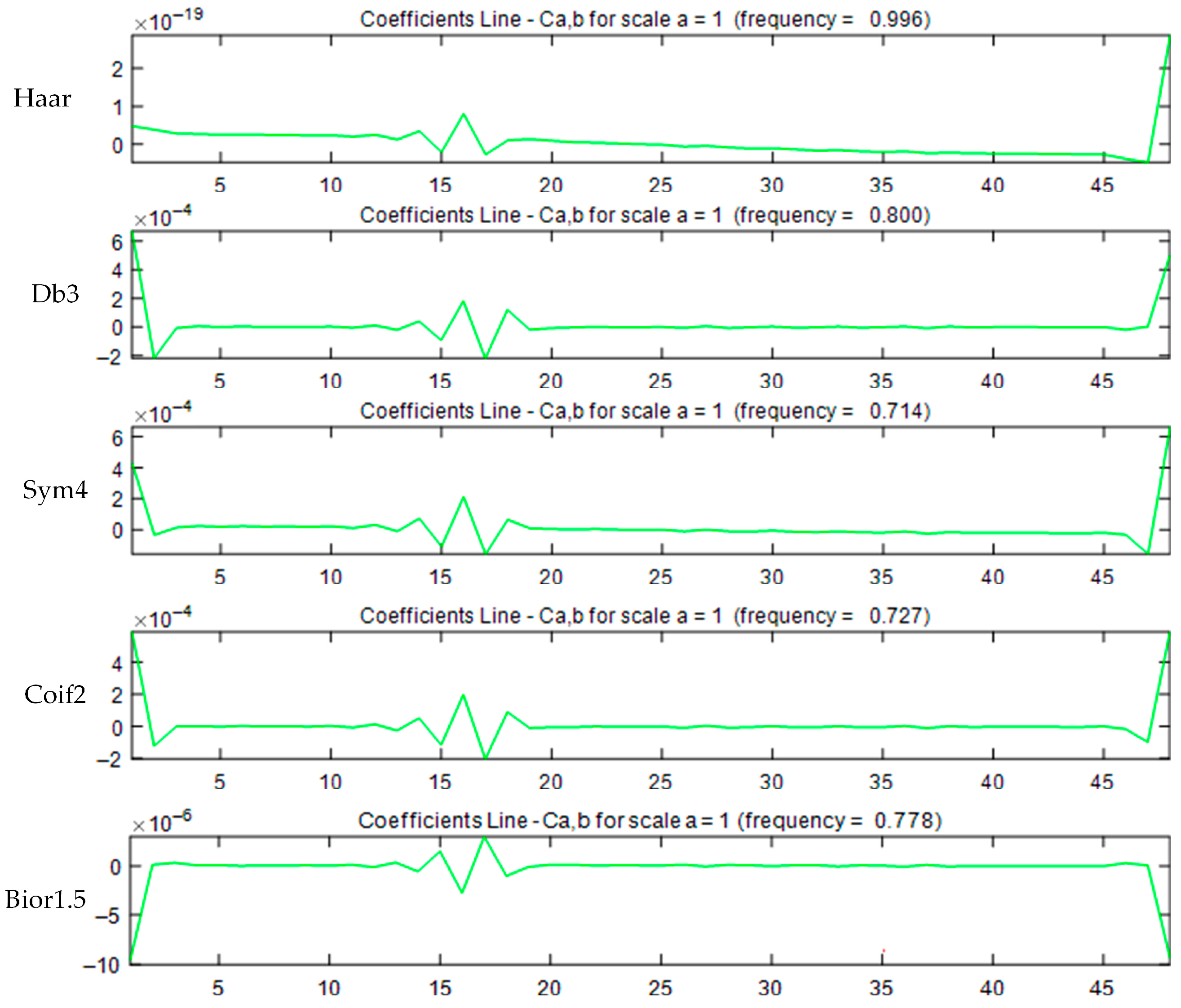
As a baseline, we first applied the conventional trial-and-error approach—still widely used in the literature—to search for the best mother wavelet. This basically involves running the transform with various candidate bases and picking the winner by visually inspecting the coefficient plots. Figure 3 illustrates the wavelet coefficients obtained using Haar, Db3, Symlet4, Coiflet2, and BiorSplines1.5, respectively. Based on the principle of wavelet singularity, all five wavelets successfully reveal a distinct singularity at 1/3 of the beam span, corresponding to the damage location. However, such qualitative assessment is incapable of rigorously identifying the optimal mother wavelet. Worse yet, it completely ignores how environmental noise distorts the signal in real-world engineering scenarios. Given these glaring blind spots, the traditional trial-and-error method falls significantly short.

Figure 3. Mother wavelet selection using the trial-and-error method under noise-free.

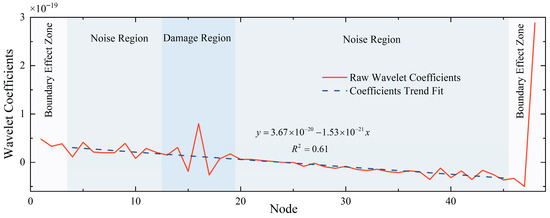
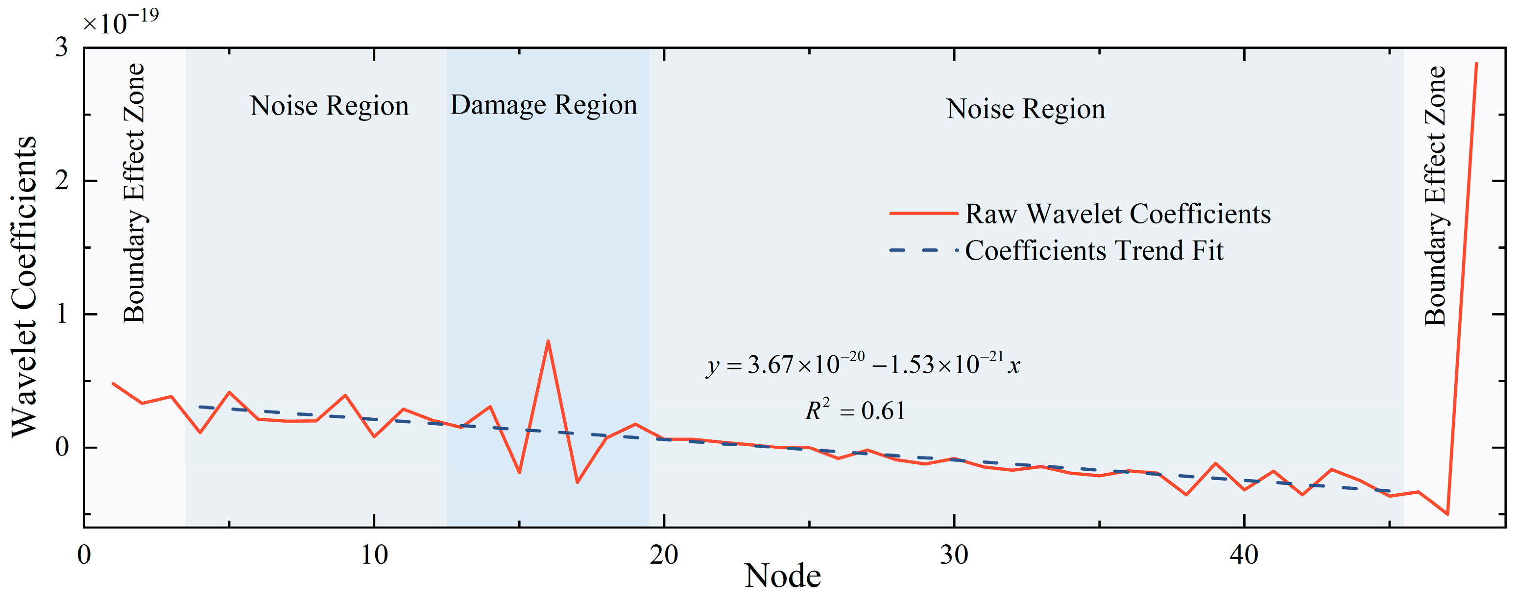
Taking the Haar wavelet as an illustrative example, the RWCI is computed under a noise level of 90 dB.

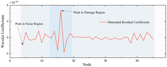
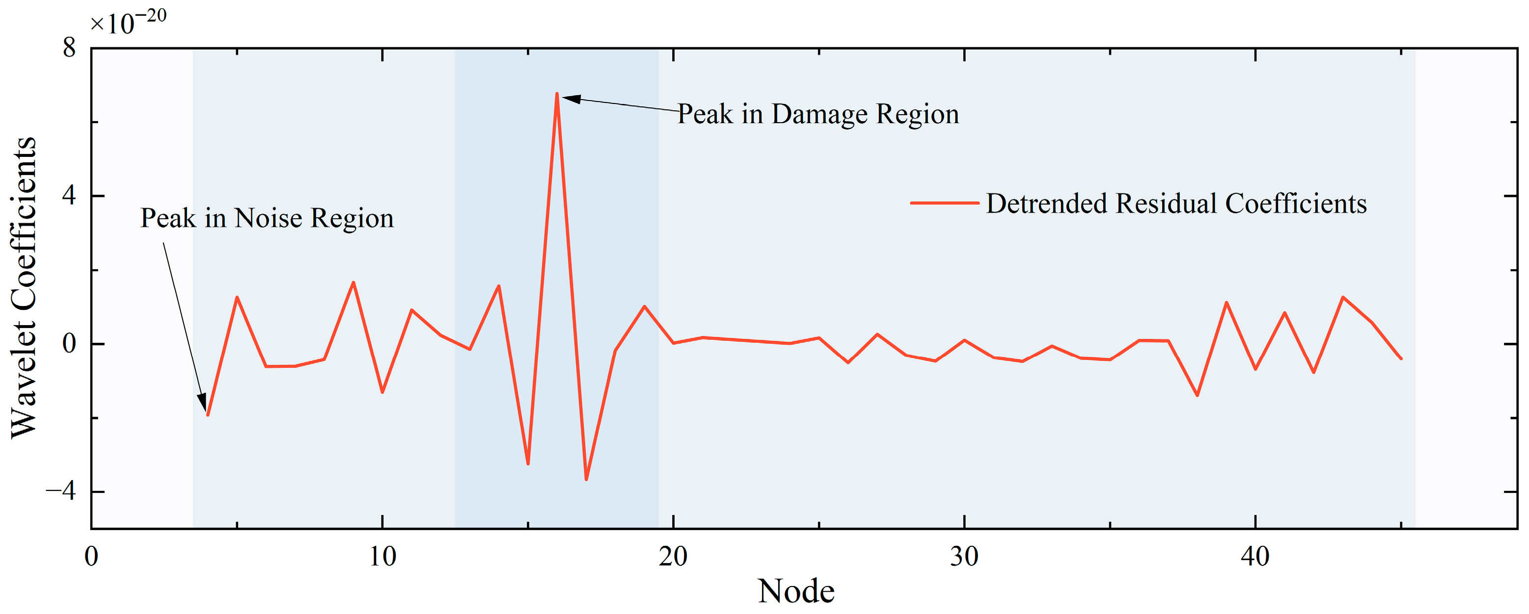
As shown in Figure 4, we kick things off by trimming away the edges of the raw wavelet coefficients to discard any regions corrupted by boundary effects. Next, we use the Least Squares Method to capture the global trend and subtract it directly from the data. This detrending step strips away the underlying curvature, leaving us with the clean residual profile you see in Figure 5. From there, calculating the RWCI is straightforward: we simply take the peak value within the actual damage zone and subtract the highest noise spike found in the background.

Figure 4. Wavelet coefficients and the global trend fit of the coefficients (Illustration of Stage 1 processing for a single-damage scenario).

Figure 5. Detrended residual coefficients.

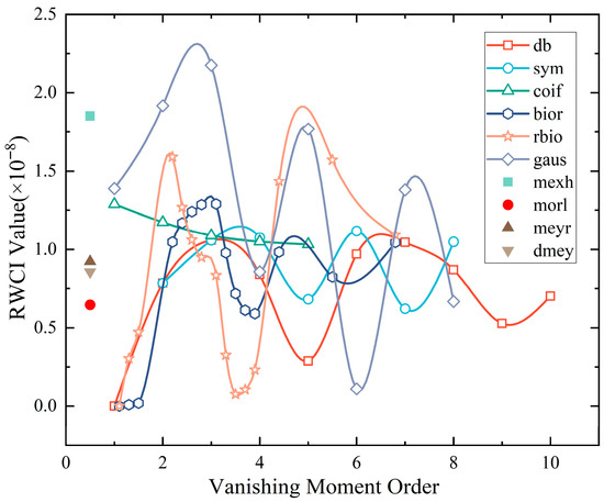
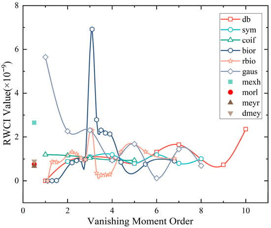
With this procedure in place, we computed the RWCI values across a broad pool of 64 mother wavelets. These candidates were selected from the Db, Sym, Coif, Bior, Rbio, and Gaus families, as well as individual wavelets including mexh, morl, meyr, and dmey. The calculations were performed under five distinct noise scenarios: noise-free, 90 dB, 80 dB, 70 dB, and 60 dB.

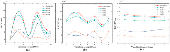
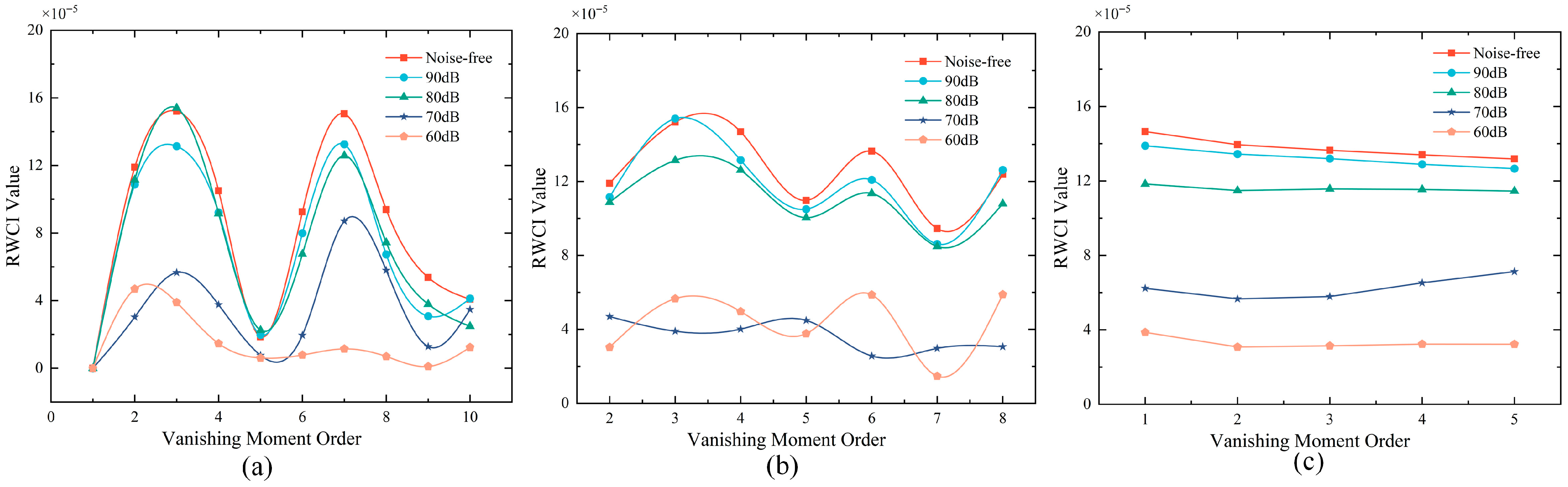
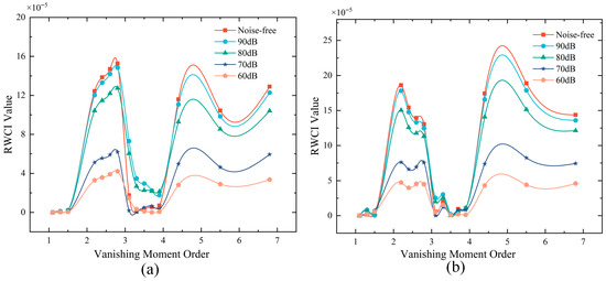
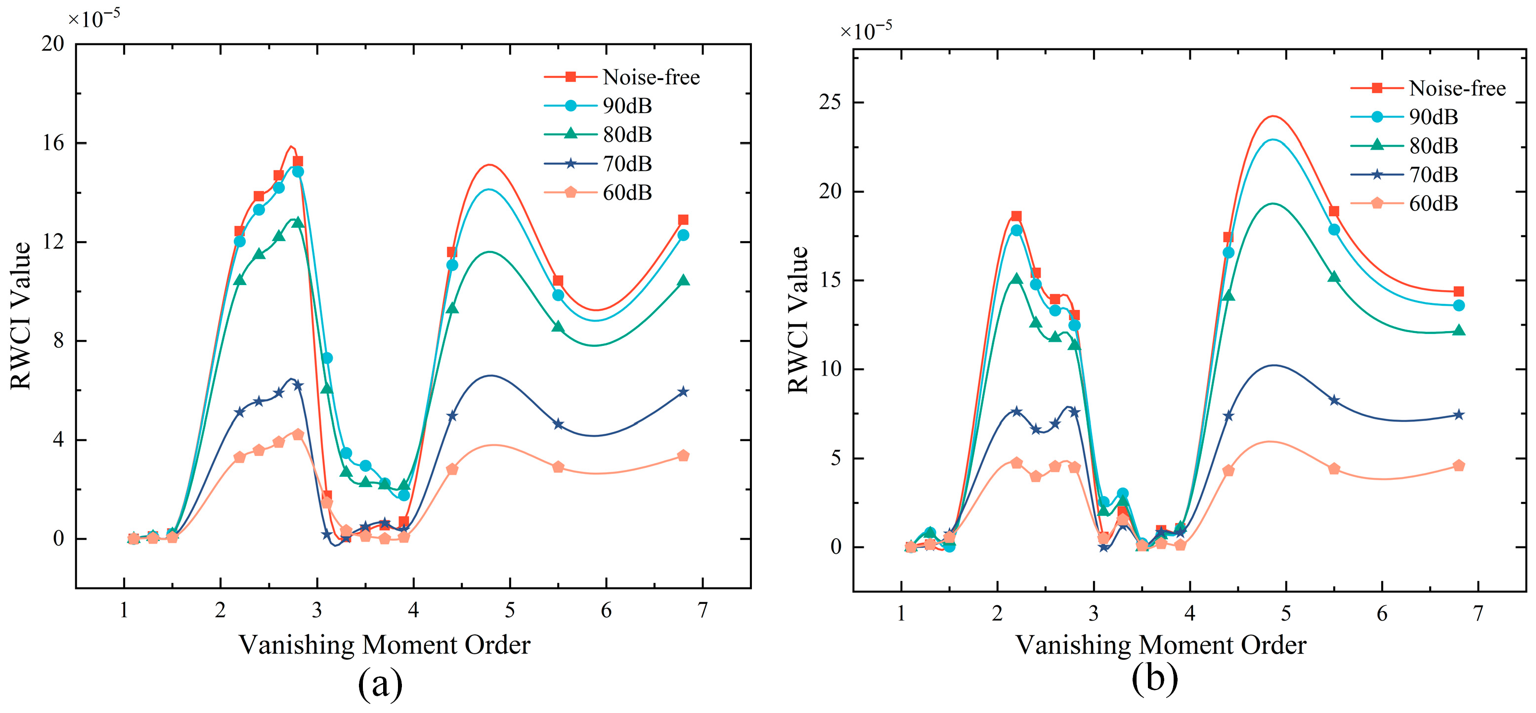
Figure 6a,b map out how the Db and Sym wavelet families perform as their vanishing moment orders increase. Interestingly, the RWCI curves for both families show a distinct ‘double-peak’ pattern, achieving local optima at lower orders (e.g., db3, sym3). This phenomenon can be interpreted through two primary mechanisms.

Figure 6. [Stage 1: Mother Wavelet Selection] Variation in the RWCI with respect to the order of vanishing moments under different noise levels for the single-damage scenario: (a) Db; (b) Sym; (c) Coif.

First, the interplay between compact support and discrete meshing. Given the relatively sparse spatial sampling of the 50-node discrete data used in this study, lower-order wavelets (such as db3) possess a shorter effective support length. This feature allows them to precisely localize the abrupt curvature change induced by the 20% stiffness reduction within a narrow spatial confinement, effectively circumventing the ‘over-smoothing’ effect. By contrast, bumping up the order to something like db10 stretches out the wavelet’s support. This wider footprint causes two major issues: it pulls in unwanted boundary interference from the clamped ends, and it physically “smears” the sharp damage singularity across neighboring elements. Naturally, this blurring effect drags down the RWCI performance.

Second, the role of symmetry in keeping phase distortion in check. Side-by-side, Sym wavelets consistently beat out their Db equivalents at the same orders, delivering much smoother performance curves. This superiority stems from the design of Sym wavelets as least asymmetric, which significantly mitigates nonlinear phase distortion during the transform. For the pulse-like damage signal resulting from the second-order difference, preserving phase linearity is critical for accurately locking onto the peak position and preventing energy leakage.

Turning to Figure 6c, the Coif series clearly struggles to generate high amplitudes across the board. The culprit here is its underlying math: Coiflets enforce vanishing moments on both their scaling and wavelet functions. That dual property might be fantastic for general data compression, but it becomes a liability for our specific needs. The resulting wavelets are simply too smooth—instead of capturing the sharp, abrupt mutations triggered by the damage, they inadvertently iron them out, flattening the very signals we are trying to catch.

Moving on to Figure 7a,b, we mapped out the performance profiles for the Bior and Rbio wavelet families. What immediately jumps out is how completely the Rbio series outshines its standard Bior counterparts. Specifically, the Rbio trajectories exhibit exceptionally high amplitudes (notably in the vicinity of rbio2.2), with RWCI values reaching 1.86 × 10⁻⁴. We can trace this massive performance boost back to the following physical mechanisms.

Figure 7. [Stage 1: Mother Wavelet Selection] Variation in the RWCI with respect to the order of vanishing moments under different noise levels for the single-damage scenario: (a) Bior; (b) Rbio.

First, the power of dual filter construction. Biorthogonal wavelets rely on a clever architecture: they use pair-wise dual filter banks. This setup allows them to hit two targets that are usually hard to reconcile—compact support and exact symmetry—at the same time. For the modal data coming off our fixed-fixed beam, this symmetry is absolutely non-negotiable. It effectively kills the “localization drift” artifacts that asymmetric bases are notorious for creating, ensuring the damage signal stays exactly where it should be.

Second, Rbio’s natural affinity for sharp mutations. The real secret to the Rbio series’ standout performance lies in its decomposition stage, where it relies on scaling functions with highly specific regularity. Because our 20% stiffness drop triggers a sharp, Dirac-like discontinuity in the modal curvature (extracted via that second-order difference), we need a wavelet that physically matches this shape. Rbio’s waveform topology fits the bill perfectly. It is practically tailor-made to reconstruct these abrupt features using a very sparse set of coefficients. Ultimately, this highly efficient energy concentration maximizes the damage signature, making it punch right through the background noise.

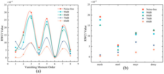
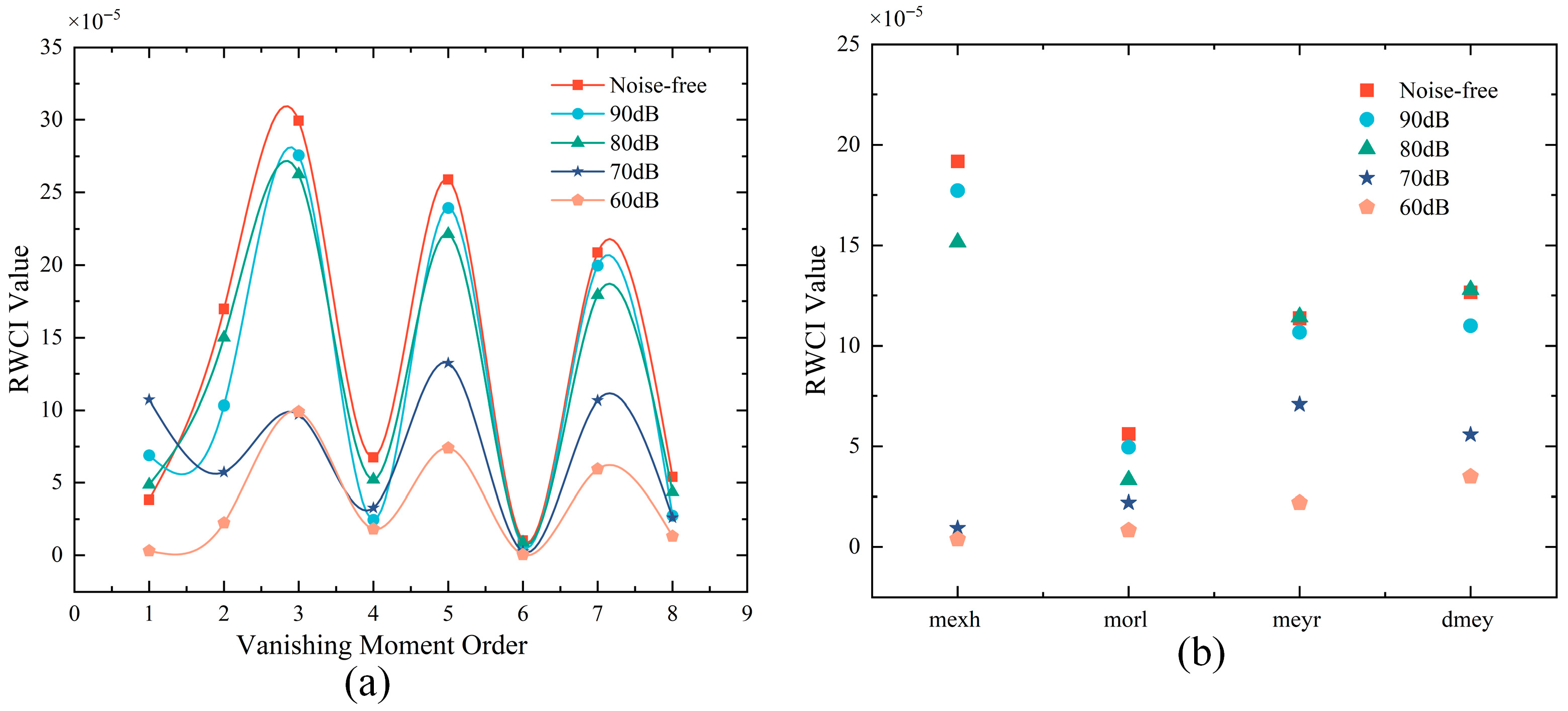
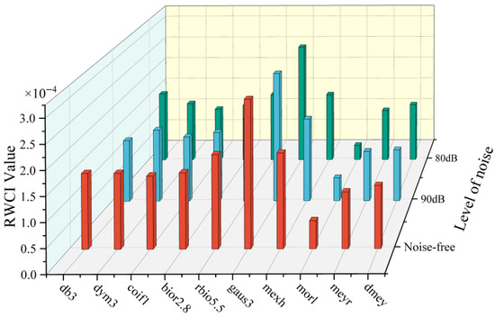
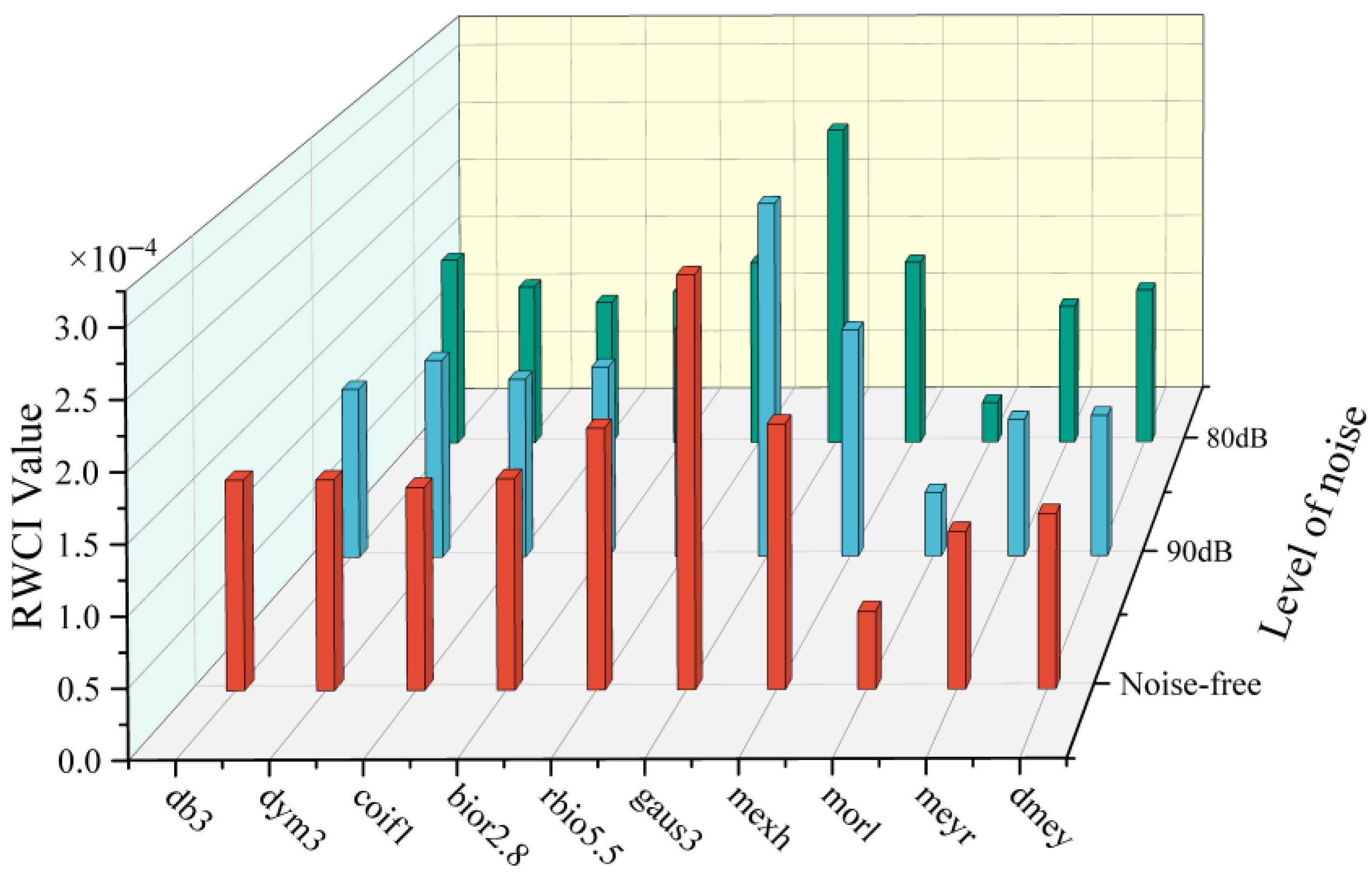
Looking at the broader comparison in Figure 8a and Figure 9, we arrive at the central finding of our work: the Gaussian family—particularly Gaus3 and mexh—stands unrivaled among all tested wavelets. Specifically, Gaus3 achieves remarkable RWCI values approximately 3.0 × 10⁻⁴ (2.99 × 10⁻⁴), while mexh also exhibits strong contrast with a peak value of 1.92 × 10⁻⁴. Crucially, both bases hold their ground exceptionally well even under severe 60 dB noise interference. We narrow this massive performance edge down to three underlying reasons:

Figure 8. [Stage 1: Mother Wavelet Selection] Variation in the RWCI with respect to the order of vanishing moments under different noise levels for the single-damage scenario: (a) Gaus; (b) mexh, morl, meyr and dmey.

Figure 9. [Stage 1: Mother Wavelet Selection] Selection of the optimal mother wavelet based on RWCI values under different noise levels for the single-damage scenario. (Red bars denote the noise-free condition; light blue bars denote the 90 dB noise level; and dark green bars denote the 80 dB noise level.)

Fundamentally, stiffness degradation manifests as an abrupt mutation in modal curvature. Since the mexh wavelet is the second derivative of the Gaussian function, and Gaus3 is the third, performing a CWT with these bases is mathematically equivalent to applying a high-order differential operator to the signal. Consequently, the Gaussian series functions as an inherent ‘curvature mutation detector’, significantly amplifying faint damage signatures.

Smoothness is paramount when processing second-order difference data, an operation that inevitably amplifies high-frequency numerical noise (evidenced by the performance drop across all wavelets at 60 dB). Unlike the jagged, fractal-like waveforms of the Db family, Gaussian wavelets possess C^∞regularity. This property allows them to act simultaneously as a feature extractor and a high-performance smoothing filter, effectively purging the noise amplified by the difference method.

Just as matched filter theory dictates, you hit the highest signal-to-noise ratio when your analyzing wavelet physically resembles the feature you are hunting for. In our case, the curvature singularity triggered by the damage usually takes the shape of a clear ‘single-peak’ or ‘double-peak’. This is practically a mirror image of the natural waveforms of Gaus3 and mexh. Thanks to this exact morphological match, these wavelets can pull out the damage signature with maximum efficiency.

At the other end of the spectrum, Figure 8b reveals that the Morlet (morl) wavelet struggles the most. The root of the problem lies in its core math: it is a complex wavelet inherently prone to heavy oscillations. While that oscillating nature is fantastic for frequency-domain analysis, it backfires completely when trying to catch transient, spatially abrupt signals like our beam damage. Instead of giving us a clean hit, it generates a mess of spurious peaks that completely throw off the identification process.

Then there is the dmey wavelet. While it does check the box for symmetry, its lack of compact support is an absolute dealbreaker here. Because it operates on a much more global scale, forcing it onto a finite-length beam practically invites massive boundary interference. These overwhelming edge effects completely blind the wavelet, stripping away its ability to pinpoint any localized structural flaws.

Tying all these observations together, the takeaway is clear: when you are trying to detect a 20% stiffness drop in fixed-fixed beams using second-order modal differences, success hinges entirely on picking the right wavelet basis. The Gaussian family stands out as the clear winner. It delivers the sharpest damage contrast—even when noise gets in the way—thanks to a perfect mix of smooth differential properties and excellent waveform matching. The Rbior series makes for a solid runner-up, striking a nice balance between keeping the phase linear (via biorthogonality) and sensitively capturing those damage singularities. On the flip side, you need to tread carefully with orthogonal wavelets like Db and Sym. If you go this route, sticking to low orders is non-negotiable—otherwise, the coarse grid will trip you up, and boundary effects will ruin the signal.

3.2. Numerical Identification of Damage Severity

The finite element model of the fixed-fixed beam was established within the MATLAB environment. The beam structure was discretized into 49 elements with 50 nodes, sequentially numbered from the left end (Node 1) to the right end (Node 50). Following the standard Euler-Bernoulli finite element formulation (consistent with the ANSYS element theory), the elemental stiffness and mass matrices were assembled to construct the global matrices.

Subsequently, the source codes for the standard DBO and the proposed ITDBO were developed in MATLAB. Given that the damage location has been preliminarily determined (via wavelet analysis), the optimization problem is simplified to identifying the damage severity of the target element, which serves as the design variable in the fitness function. The natural frequencies and mode shapes derived from the numerical model are substituted into the objective function to minimize the error against the measured data.

To rigorously mitigate the stochastic nature of meta-heuristic algorithms, both DBO and ITDBO were executed for 10 independent runs on the same computing platform. To ensure a fair and comprehensive evaluation of robustness, no outliers were excluded from the statistical analysis of the results.

The population size and maximum number of iterations were set to N = 30 and T = 50, respectively, representing an optimal trade-off between computational efficiency and identification accuracy. The internal demographic distribution of the dung beetles was maintained at standard fixed values without modification. Specifically, the proportions for ball-rolling, thieving, brood, and foraging beetles were allocated as 20%, 40%, 20%, and 20%, respectively. Furthermore, the search space for the damage variables was constrained to ensure physical feasibility: the upper bound (UB), representing the maximum stiffness reduction, was capped at 80%, while the lower bound (LB) was fixed at 0%.

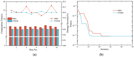
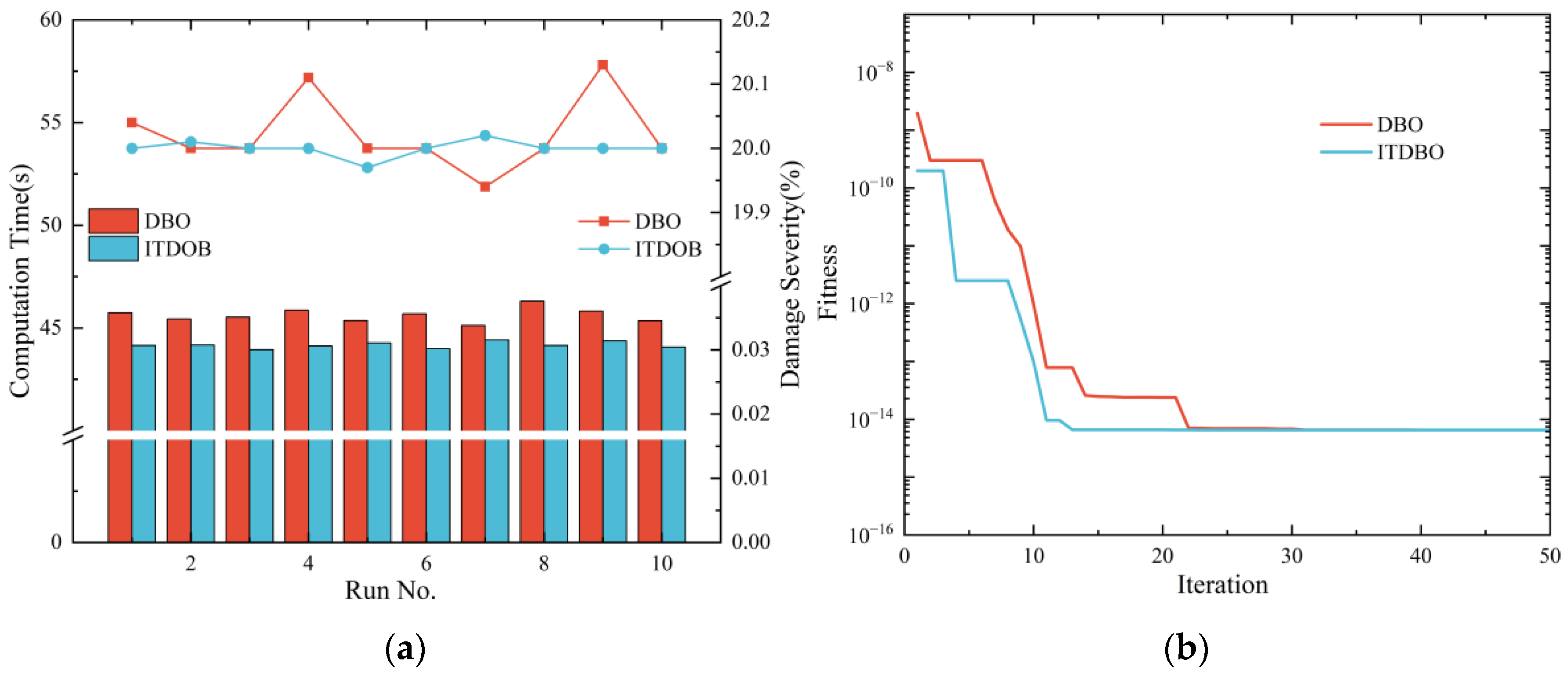
Looking at the statistical breakdown across 10 independent runs in Figure 10a, ITDBO’s robustness really stands out. It nails the actual 20% damage extent almost perfectly, showing a near-zero standard deviation. The standard DBO, on the other hand, struggles with volatility, bouncing anywhere between 19.9% and 20.1%. What is even better is that despite running extra mutation steps, ITDBO actually clocks in slightly faster—averaging 44.165 s compared to DBO’s 45.622 s. This lean computational footprint makes it a highly practical choice for time-sensitive structural health monitoring.

Figure 10. [Stage 2: Damage Quantification] Identification results of the beam damage severity obtained by DBO and ITDBO for the single-damage scenario: (a) Computation time and damage severity; (b) Average convergence curves.

Switching over to the fitness evolution curves in Figure 10b, the difference in convergence speed is striking. ITDBO easily breaks out of local optima and plunges straight to the theoretical minimum (10⁻¹⁴) in under 12 iterations. The standard DBO trails behind with a much lazier descent, needing nearly double the iterations (around 23) just to stabilize. We credit this rapid convergence directly to the adaptive t-distribution perturbation. By actively injecting diversity into the population, it forces the search trajectory to aggressively lock onto the global optimum.

3.3. Sensitivity and Robustness Analysis

This section investigates the robustness of the proposed RWCI strategy under three critical conditions: limited spatial resolution, low-severity damage, and parameter variability. The numerical model employed in this sensitivity analysis retains the identical material properties and boundary conditions as described in Section 3.1.

3.3.1. Detection of Closely Spaced Damage

To push the spatial resolution of our method to the limit, we set up a dual-damage scenario with two closely spaced defects. We introduced 15% stiffness reductions at Elements 18 and 21, leaving just two healthy elements between them. This tight configuration is a classic stress test for resolving adjacent damage sources

Figure 11 plots the RWCI indices across our 64 candidate wavelets for this dual-damage case, heavily masked by 80 dB noise. Just as we saw in the single-damage tests, gaus3 once again claims the top spot. Its performance remains rock-solid, proving that its superior contrast isn’t just a fluke.

Figure 11. [Stage 1: Localization] Comparison of RWCI indices obtained using different wavelet bases for the closely spaced damage scenario (Elements 18 and 21) under 80 dB noise conditions.

Looking closely at Figure 12, the RWCI profile carves out a very clear ‘M-shaped’ double peak right over Elements 18 and 21—even while fighting through the 80 dB noise interference. Sure, the heavy noise stirs up some minor background ripples in the healthy zones, but our 50% adaptive threshold easily keeps those artifacts in check. In fact, this scenario really highlights why that thresholding strategy is so vital. It does much more than just filter noise. Taking a cue from the Full Width at Half Maximum (FWHM) principle, the threshold effectively slices off the overlapping, low-amplitude ‘skirts’ of the adjacent wavelet coefficients. Because of this clean cutoff, the two damage sources emerge as distinct, independent high-energy cores instead of blurring together into one massive, confusing blob. Ultimately, this proves our framework can deliver razor-sharp spatial resolution and dodge false alarms, no matter how poor the signal-to-noise ratio gets.

Figure 12. [Stage 1: Localization] Wavelet coefficients using the gaus3 mother wavelet for the closely spaced damage scenario (Elements 18 and 21) under 80 dB noise conditions.

3.3.2. Detection Limit for Incipient Damage

Spotting incipient damage is notoriously difficult because the SNR always works against you. To see how our method handles this extreme end of the spectrum, we dialed the stiffness reduction at Element 18 way down to just 2%. We kept the Gaussian white noise at 80 dB SNR to mimic high-fidelity measurement conditions.

Turning to Figure 13, the detection results for this tiny defect using the gaus3 wavelet tell a very different story. Unlike the crystal-clear peaks we saw in the 15% damage case, the wavelet coefficients here essentially flatline across the damage location. This happens because of the classic “Signal-Masking Effect.” Even though an 80 dB SNR represents a relatively quiet environment, the curvature singularity triggered by a mere 2% defect is simply too faint. Despite the RWCI’s band-pass filtering capabilities, the spectral energy of that tiny singularity completely drowns in the ambient noise floor.

Figure 13. [Stage 1: Localization] Wavelet coefficients using the gaus3 mother wavelet for the incipient damage scenario (Elements 18) under 80 dB noise conditions.

On top of that, our 50% adaptive threshold kicks in exactly as designed. Because we built it to guarantee zero false positives, it ruthlessly filters out this weak signal right alongside the background fluctuations. This brings us to a fundamental trade-off in structural health monitoring: sensitivity versus robustness. Sure, we could lower the threshold to catch that 2% damage, but doing so would open the floodgates to unacceptable false alarms from random noise artifacts. Ultimately, this test empirically proves that under these specific noise conditions, our method’s Limit of Detection (LOD) sits somewhere above the 2% mark.

Because the true damage signature is completely masked here, the RWCI variations across the different mother wavelets in Figure 14 look entirely different from the consistent patterns we saw earlier. What you are seeing in those values is just random noise artifacts dominating the structural features. For that reason, trying to use this specific 2% scenario to pick the “optimal” wavelet is practically meaningless.

Figure 14. [Stage 1: Localization] Comparison of RWCI indices obtained using different wavelet bases for the incipient damage scenario (Elements 18) under 80 dB noise conditions.

3.3.3. Stability Regarding Parameter Definition

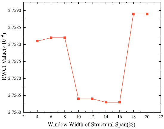
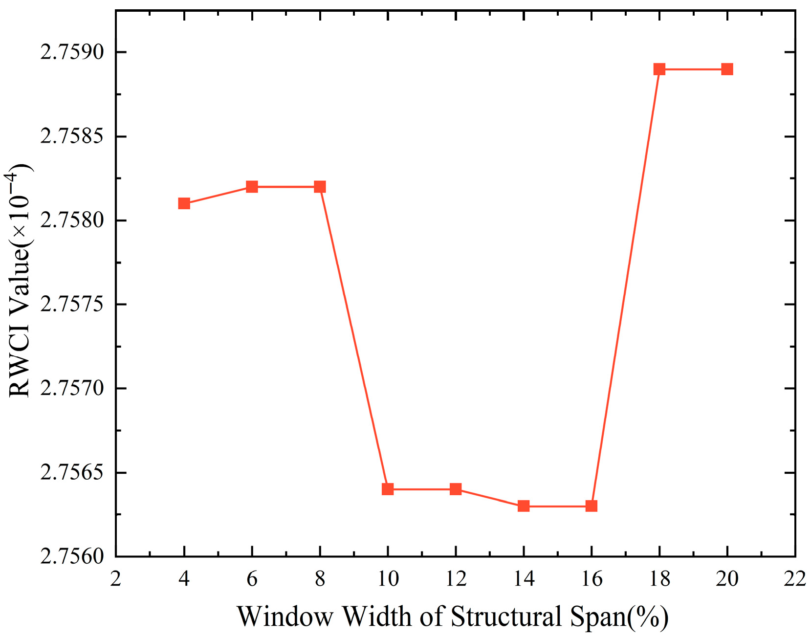
To evaluate the dependence of the RWCI algorithm on the definition of the damage region (${\Omega }_{dmg}$), a parametric study was conducted by varying the window width from 4% to 20% of the structural span. The damage scenario adopted for this parametric study remains consistent with the base line case described in Section 3.1 (specifically, a 20% stiffness reduction at Element 17). Without loss of generality, the analysis is performed using the optimal wavelet basis (gaus3) under the standard 80 dB noise condition. The variation in the RWCI with respect to the window width is illustrated in Figure 15.

Figure 15. [Stage 1: Localization] Variation in the RWCI with respect to the defined window width (ranging from 4% to 20% of the structural span) for the single-damage scenario under 80 dB noise.

The curve exhibits a characteristic “step-wise concave” behavior. The step-like transitions arise from the finite element discretization of the beam. As the continuous window ratio increases, the effective number of discrete elements included in the calculation changes incrementally (e.g., from 3 to 4 elements), leading to discrete jumps in the index value. Despite these morphological fluctuations, the overall variation remains within a narrow range (less than 0.1%). This result demonstrates that the algorithm is virtually invariant to the specific definition of the damage region boundaries. The choice of a 10% window is therefore proven to be not only physically reasonable but also numerically highly robust, ensuring consistent damage quantification results regardless of minor parameter perturbations.

4. Experimental Validation

4.1. Damage Localization

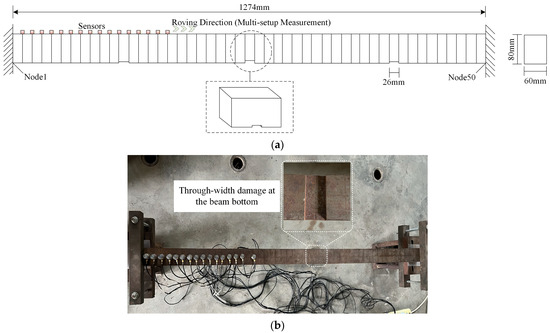
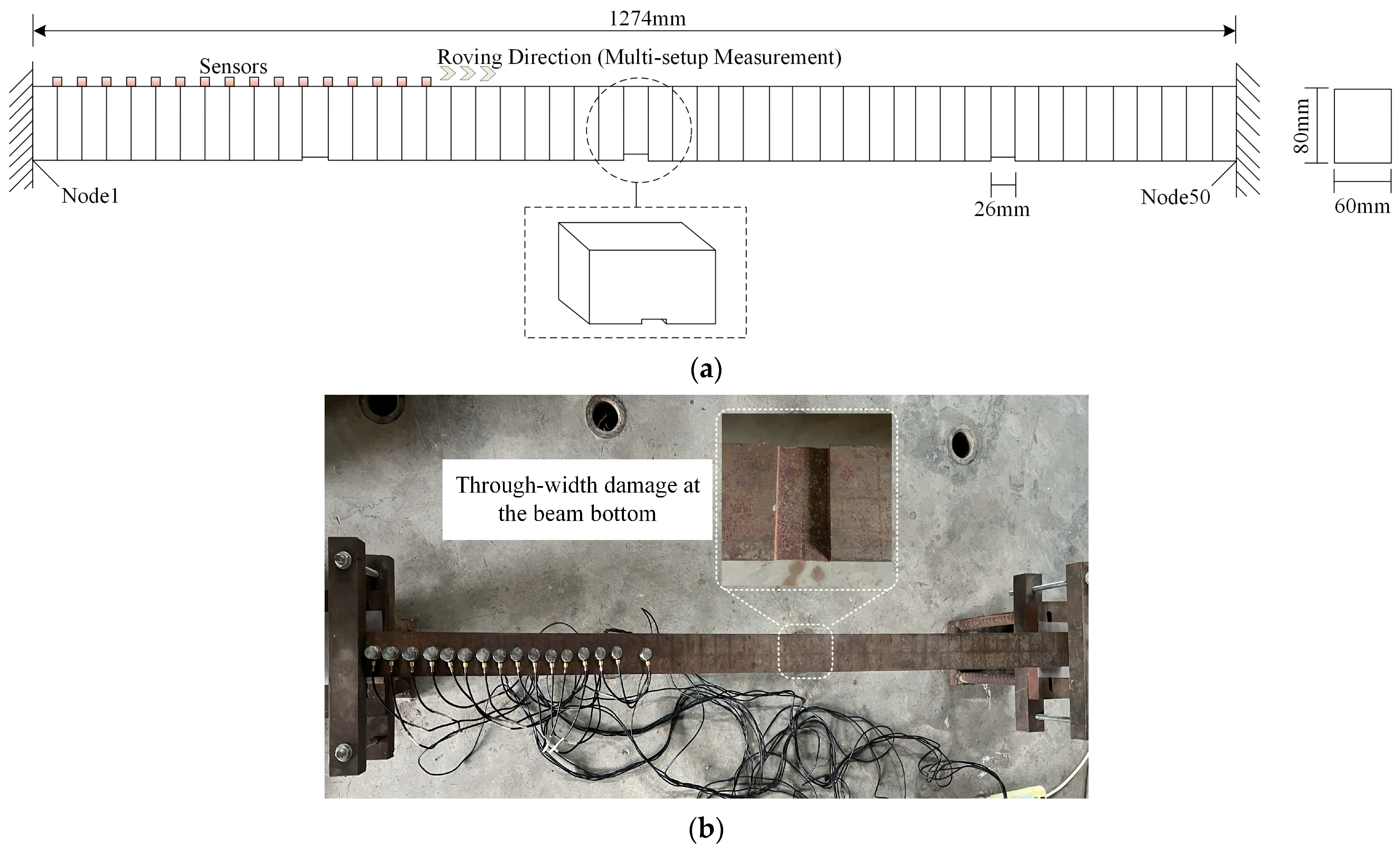
Following the numerical verification of the ITDBO algorithm’s efficacy in detecting edge damage within fixed-fixed beam, experimental trials were conducted to substantiate its applicability to real-world structures. The experimental specimen consists of a fixed-fixed beam subject to a through-width rectangular notch with a width of 26 mm, as illustrated in Figure 16. The material parameters of the beam are consistent with those presented in Section 3.1. The depth of this notch is correlated with the damage severity index defined in Equation (18).

Figure 16. Experimental setup of the fixed-fixed beam: (a) schematic diagram illustrating the sensor arrangement, roving measurement strategy, and geometric dimensions; (b) photograph of the actual test specimen with installed piezoelectric accelerometers.

To capture the structure’s dynamic response, we wired up 16 high-sensitivity 1A110E IEPE piezoelectric accelerometers. To perfectly mirror our numerical grid, we physically marked the beam into 26 mm segments. Of course, dealing with real hardware means accounting for physical constraints—so to comfortably fit the sensors near the clamped boundaries, we left a practical 13 mm offset at both ends. All sensors were aligned along the longitudinal mid-axis of the beam’s upper surface. Since we needed to map all 50 nodes but only had a 16-sensor array on hand, we relied on a classic roving sensor setup. We ran the test in multiple batches, shifting the sensors along the beam while keeping a single reference sensor permanently fixed to guarantee tight phase synchronization. For the structural excitation, we struck the beam using a GST (LC-04A) impact hammer under the unmeasured-force method. Finally, it was just a matter of feeding the raw acceleration data into our DH5922D system to cleanly extract those crucial fundamental displacement mode shapes.

Once we pulled the first-order displacement modes from the test rig, we immediately derived the strain modes using the standard second-order difference method. From there, we piped the signals straight into MATLAB 2019b. Relying on its Wavelet Toolbox, we ran a CWT powered by our top-performing gaus3 basis. This move effectively scrubs out the noise and isolates the clean wavelet coefficients we need. To verify the algorithm’s capability in handling complex conditions, a multi-damage case is introduced where Element 12 (4.9%), Element 25 (18.6%), and Element 40 (9.7%) are damaged simultaneously.

Figure 17 maps out the wavelet coefficients derived from our experimental first-order displacement modes, processed with the ‘gaus3’ basis. As observed in the figure, the wavelet coefficients exhibit distinct singularity peaks at three specific locations along the beam span. These peaks correspond precisely to the indices of Element 12, Element 25, and Element 40, successfully identifying the pre-set damage locations.

Figure 17. [Stage 1: Localization] Wavelet coefficient diagram of the beam under the multi-damage scenario (Experimental result).

What is even more impressive is that the signal strength isn’t random—it scales directly with the severity of the stiffness cut. The peak at Element 25 dominates the landscape, matching its massive 18.6% damage level. Element 40 follows with a moderate spike (9.7%), while the signal at Element 12 is much more subdued, perfectly mirroring that minor 4.9% nick. This result demonstrates that the proposed method utilizing Gaussian wavelet transform can effectively detect simultaneous multiple damages and qualitatively reflect the relative severity of the defects, even under experimental noise conditions.

We do need to be upfront about one critical limitation: the RWCI algorithm lives and dies by its spatial sampling. Because the wavelet transform basically acts as a strict spatial high-pass filter, your sensor layout matters immensely. If you space your sensors too far apart, you run the risk of spatial aliasing. Even worse, the high-frequency singularity triggered by a local stiffness drop could simply fall right through the cracks, slipping entirely unnoticed between two measurement points. In this study, the spatial resolution of 26 mm (L/49) was sufficient to capture the damage features. For practical applications on larger structures where dense sensor arrays are costly, roving measurement techniques (as employed in this experiment) or optimal sensor placement strategies focusing on critical regions are recommended to maintain sufficient local density for wavelet analysis.

4.2. Identification of Damage Severity

This section validates the comprehensive performance of ITDBO by benchmarking it against five mainstream metaheuristics, covering classical, mathematical, and physics-based paradigms. To guarantee experimental fairness, a unified computing environment was established. Specifically, convergence stagnation was observed in the Improved PSO (IPSO) under small population constraints, a uniform population size of N = 60 and a maximum iteration limit of T = 80 were applied to all algorithms.

The internal parameters for the comparative algorithms (IPSO, GWO, SCA, RIME, and IGA) were initialized according to the default configurations suggested in their respective original literature. Specifically, for IPSO [13], the inertia weight w decays linearly from 0.9 to 0.4, with c₁ = c₂ = 2.0. For the IGA [15], the key parameters are set as follows: crossover probability = 0.5, mutation probability = 0.01, cloning rate = 0.6, and cloning inhibition rate = 0.01. Similarly, the convergence factor a in both SCA and GWO linearly decreases from 2 to 0, while the soft-frost coefficient in RIME is fixed at w_rime = 5. For the ITDBO algorithm, apart from the specific introduction of Bernoulli chaos initialization and t-distribution mutation, all basic parameters align with the standard DBO setup detailed previously. By strictly enforcing these standard settings across the board, we ensure that any performance edge ITDBO shows comes purely from our structural upgrades—not from tweaking numbers to stack the deck.

The numerical modeling and calculations were implemented within the MATLAB environment. With the framework set, we brought in the intelligent algorithms to tackle the damage quantification task. To make sure our findings were statistically bulletproof—not just a lucky break—we ran 10 independent trials for each algorithm. We kept the computational conditions strictly identical across every single run, recording the full dataset for a rigorous performance breakdown. The comprehensive identification results under the multiple damage scenario are visualized in Table 1 and Figure 18.

Table 1. Comparison of damage identification accuracy and computational efficiency among different intelligent algorithms.

Algorithm	Elapsed Time (s)	Element 12 (%)	Element 25 (%)	Element 40 (%)
IPSO	276.33 ± 2.13	4.9 ± 0.076	18.6 ± 0.336	9.7 ± 0.261
GWO	279.95 ± 3.03	4.902 ± 0.223	18.607 ± 0.155	9.699 ± 0.007
SCA	285.3 ± 4.31	4.909 ± 0.049	18.511 ± 0.118	9.754 ± 0.074
RIME	273.12 ± 0.69	4.924 ± 0.098	18.586 ± 0.078	9.712 ± 0.04
ITDBO	267.83 ± 1.71	4.9 ± 0.06	18.595 ± 0.015	9.716 ± 0.049
IGA	285.71 ± 1.83	4.922 ± 0.056	18.578 ± 0.177	9.672 ± 0.311

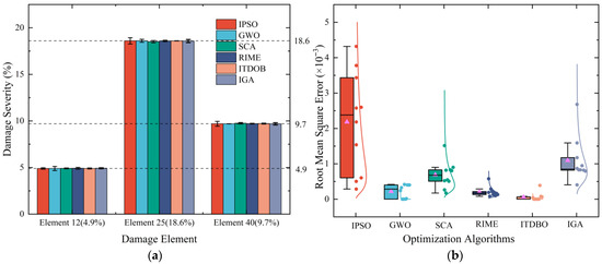
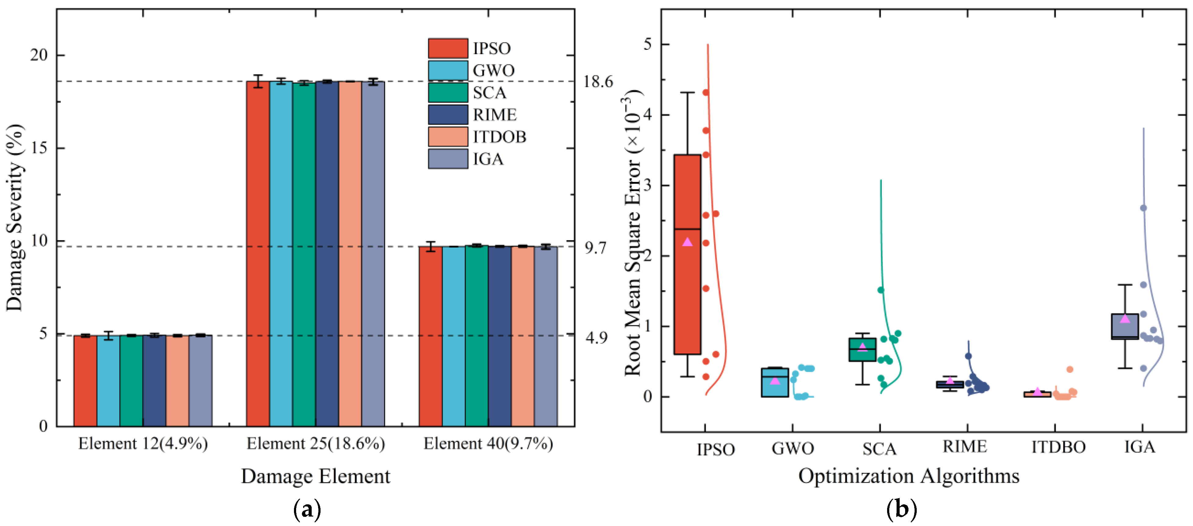
Figure 18. [Stage 2: Damage Quantification] Statistical performance analysis of the six optimization algorithms under the multiple damage scenario: (a) damage severity; (b) Root Mean Square Error (RMSE).

Looking at the identification accuracy in Figure 18a, the histogram tells us right away that all six algorithms can successfully flag the damage locations. However, distinct differences are observed in the precision of severity quantification. The results obtained by the proposed ITDBO align almost perfectly with the benchmark dashed lines across all three damage locations (Elements 12, 25, and 40). Crucially, when compared with our previous works, the IPSO [13] exhibits noticeable deviations from the true values with the largest error bars, reflecting high instability. The IGA [15] achieves improved accuracy over IPSO but still displays visible fluctuations. In contrast, the error bars associated with ITDBO are visibly shorter compared to those of IPSO, IGA and SCA, indicating superior consistency across repeated trials.

Turning to the statistical robustness in Figure 18b, the box plots really expose the underlying performance gaps. The IPSO algorithm exhibits the largest RMSE fluctuation, with a broad probability distribution and high median error, suggesting poor stability. The IGA [15] shows a relatively better distribution benefiting from immune diversity, yet it still contains outliers indicative of occasional stagnation. In contrast, the ITDBO algorithm achieves the lowest mean RMSE and the most compact distribution density, which is heavily concentrated near zero. This narrow distribution range signifies that ITDBO possesses exceptional convergence stability and is less susceptible to stochastic randomness compared to GWO, SCA, IGA and RIME.

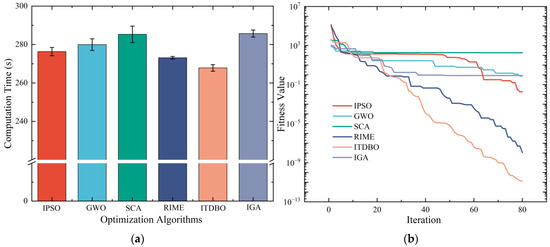
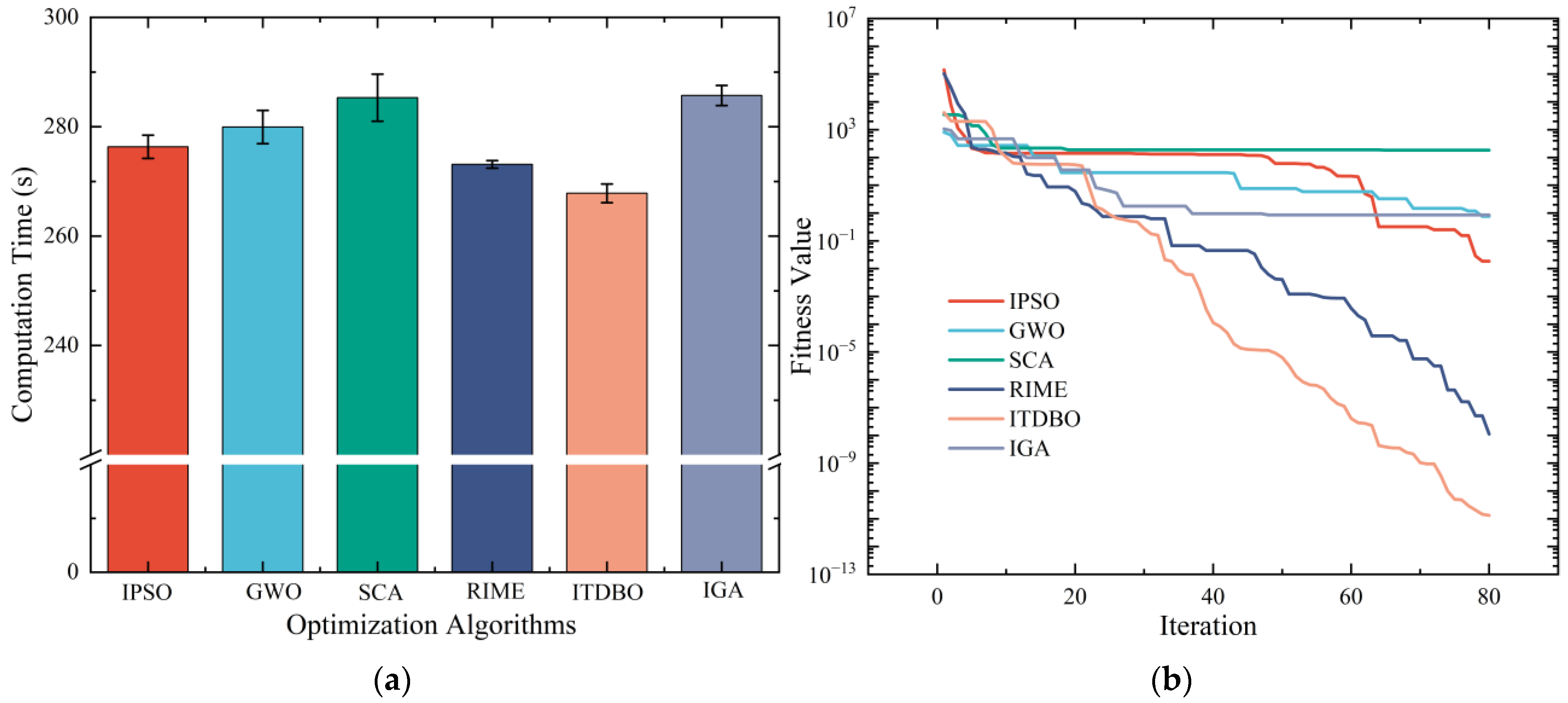
Figure 19 tackles the performance showdown from two distinct angles: time complexity and convergence behavior. As illustrated in Figure 19a, the computation time is a critical metric for practical engineering applications. The bar chart reveals that the ITDBO algorithm achieves the highest efficiency, with a minimum average execution time of 267.83 s. On the flip side, IGA gets visibly bogged down (285.71 s) by its heavy clonal selection and concentration mechanisms. Interestingly, even IPSO (276.33 s), which theoretically has a simpler architecture, fails to gain any real speed advantage over IGA. Consequently, ITDBO stands out as the fastest algorithm in this study, proving its superiority in minimizing computational overhead without compromising the complexity required for high-precision search.

Figure 19. [Stage 2: Damage Quantification] Evaluation of computational efficiency and evolutionary convergence performance. (a) Comparison of average computation time over 10 independent runs; (b) Convergence history of the best fitness values over 80 iterations.

The convergence curves in Figure 19b further elucidate the search mechanism. IPSO comes out of the gate strong with a steep initial drop, but it hits a wall way too early, flatlining around a fitness of 10⁻¹. This confirms that the linear inertia weight strategy adopted in [13], while an improvement over standard methods, is still insufficient to help particles escape local optima in complex multi-damage scenarios. The IGA enters a prolonged state of stagnation around 10⁰, lacking the drive for deep exploitation.

Then there is ITDBO. Instead of stalling out, it keeps digging deeper iteration after iteration. It cleanly punches through the exact same local optima that ensnared IPSO and IGA, driving the fitness all the way down to a razor-sharp 10⁻¹¹. This confirms that the improved strategies in ITDBO successfully mitigate the risk of stagnation and significantly enhance global search efficiency.

The disparity in convergence stability, as evidenced by the boxplots in Figure 18b, can be attributed to the algorithmic mechanisms for handling population diversity. Even improved metaheuristics like IPSO and SCA rely heavily on the ‘best-so-far’ guidance. In the high-dimensional landscape of damage identification, this often leads to a rapid loss of diversity, causing the population to cluster prematurely around local optima (stagnation). The superior stability of ITDBO stems from its t-distribution mutation operator. Unlike the static update rules of DBO, this operator utilizes the heavy-tailed property of the t-distribution to inject significant perturbations when the algorithm tends to stagnate. This mechanism effectively ‘resets’ the search momentum, allowing the optimizer to escape local traps and consistently locate the true global minimum.

5. Conclusions

In this study, we developed a robust, two-stage damage identification framework for beam structures that actively cuts through the noise. By pairing our new Residual-Based Wavelet Contrast Index (RWCI) to hunt down the perfect mother wavelet, with our Improved t-distribution Dung Beetle Optimizer (ITDBO) to crunch the severity numbers, we built a pipeline designed for both precision and speed. After putting the framework through its paces in both numerical simulations and physical steel beam tests, we arrive at four core conclusions:

(1) RWCI Takes the Guesswork Out of Wavelet Selection: Instead of relying on trial and error, the RWCI provides a hard, quantitative metric to adaptively crown the optimal mother wavelet. It definitively flagged the Gaussian family—specifically ‘gaus3’—as the ultimate tool for the job. Because its natural shape perfectly mirrors the damage-induced singularity, gaus3 drastically boosts the signal-to-noise ratio, locking onto defects with pinpoint accuracy even when the data is heavily corrupted by noise.

(2) ITDBO Crushes the Optimization Bottleneck: Standard DBO has its limits, so we supercharged it with Bernoulli chaotic mapping and an adaptive t-distribution perturbation. The statistical payoff is massive. Compared to mainstream heavyweights like IPSO, GWO, SCA, IGA, and RIME, ITDBO simply refuses to get stuck in premature convergence. It consistently punches through local traps to locate the true global optimum, driving quantification errors down to practically zero.

(3) Trying to optimize an entire structure at once is a computational nightmare. Our two-stage strategy sidesteps this completely. By letting the wavelet localization narrow down the exact search zones first, ITDBO only has to focus on the damaged regions. Our multi-damage experiments proved that this targeted approach is incredibly lean—slashing the required iterations—while remaining highly robust for practical structural health monitoring.

(4) Limitations and Future Work: While the proposed framework demonstrates robust performance, it is important to acknowledge certain limitations inherent to laboratory-scale validation. First, the experimental tests were conducted on a scaled beam with idealized fixed boundaries and single-damage scenarios. Real-world civil structures often exhibit semi-rigid connections, complex environmental noise, and potentially multiple damage sites, which were not fully simulated in this study. Despite these constraints, the framework holds significant promise for broader applications in complex structural systems, such as high-rise buildings and bridge girders. Since these structures are principally assemblies of load-bearing members, the core principle of RWCI—detecting local curvature anomalies—remains valid for the constituent 1D-dominant components within these systems. However, applying the method to such complex geometries may require adaptive modification of the trend-removal strategy to account for continuity constraints at joints. Consequently, future work will focus on validating the method on these complex structural forms, investigating its efficacy under varying boundary conditions, and extending the optimization stage to address multi-damage identification challenges.

References

- Deng, Z.; Huang, M.; Wan, N.; Zhang, J. The Current Development of Structural Health Monitoring for Bridges: A Review. Buildings 2023, 13, 1360. [Google Scholar] [CrossRef] [Scilit]
- Zhang, J.; Huang, M.; Wan, N.; Deng, Z.; He, Z.; Luo, J. Missing Measurement Data Recovery Methods in Structural Health Monitoring: The State, Challenges and Case Study. Measurement 2024, 231, 114528. [Google Scholar] [CrossRef] [Scilit]
- Huang, M.S.; Ling, Z.Z.; Sun, C.; Lei, Y.Z.; Xiang, C.Y.; Wan, Z.H.; Gu, J.F. Two-Stage Damage Identification for Bridge Bearings Based on Sailfish Optimization and Element Relative Modal Strain Energy. Struct. Eng. Mech. 2023, 86, 715–730. [Google Scholar]
- Zhao, J.W.; Zhou, Z.; Guan, D.Q.; Guo, J. A Wavelet Based Data Coupling Method for Spatial Damage Detection in Beam-Type Structures. PLoS ONE 2023, 18, e0290265. [Google Scholar] [CrossRef] [Scilit]
- Monti, G.; Rabi, R.R.; Marella, L.; Proietti, S.T. Data-Driven Decision Support System for the Safety Management of Railway Bridge Networks. Reliab. Eng. Syst. Saf. 2025, 262, 111202. [Google Scholar] [CrossRef] [Scilit]
- Hou, R.R.; Xia, Y. Review on the New Development of Vibration-Based Damage Identification for Civil Engineering Structures: 2010–2019. J. Sound Vib. 2021, 491, 115741. [Google Scholar] [CrossRef] [Scilit]
- Fan, W.; Qiao, P. Vibration-Based Damage Identification Methods: A Review and Comparative Study. Struct. Health Monit. 2011, 9, 83–111. [Google Scholar]
- Zhang, H.; Sun, J.; Rui, X.B.; Liu, S. Delamination Damage Imaging Method of Cfrp Composite Laminate Plates Based on the Sensitive Guided Wave Mode. Compos. Struct. 2023, 306, 116571. [Google Scholar] [CrossRef] [Scilit]
- Rabi, R.R.; Vailati, M.; Monti, G. Effectiveness of Vibration-Based Techniques for Damage Localization and Lifetime Prediction in Structural Health Monitoring of Bridges: A Comprehensive Review. Buildings 2024, 14, 1183. [Google Scholar] [CrossRef] [Scilit]
- Saadatmorad, M.; Talookolaei, R.-A.J.; Pashaei, M.-H.; Khatir, S.; Wahab, M.A. Pearson Correlation and Discrete Wavelet Transform for Crack Identification in Steel Beams. Mathematics 2022, 10, 2689. [Google Scholar] [CrossRef] [Scilit]
- Katunin, A.; Lopes, H.; dos Santos, J.V.A. Identification of Multiple Damage Using Modal Rotation Obtained with Shearography and Undecimated Wavelet Transform. Mech. Syst. Signal Process. 2019, 116, 725–740. [Google Scholar] [CrossRef] [Scilit]
- Xia, C.X.; Liu, C.G. Identification and Representation of Multi-Pulse near-Fault Strong Ground Motion Using Adaptive Wavelet Transform. Appl. Sci. 2019, 9, 259. [Google Scholar] [CrossRef] [Scilit]
- Strömbergsson, D.; Marklund, P.; Berglund, K.; Saari, J.; Thomson, A. Mother Wavelet Selection in the Discrete Wavelet Transform for Condition Monitoring of Wind Turbine Drivetrain Bearings. Wind Energy 2019, 22, 1581–1592. [Google Scholar] [CrossRef] [Scilit]
- Pothisarn, C.; Klomjit, J.; Ngaopitakkul, A.; Jettanasen, C.; Asfani, D.A.; Negara, I.M.Y. Comparison of Various Mother Wavelets for Fault Classification in Electrical Systems. Appl. Sci. 2020, 10, 1203. [Google Scholar] [CrossRef] [Scilit]
- Rabi, R.R.; Monti, G. Genetic Algorithm-Based Model Updating in a Real-Time Digital Twin for Steel Bridge Monitoring. Appl. Sci. 2025, 15, 4074. [Google Scholar] [CrossRef] [Scilit]
- Guo, J.; Guan, D.Q.; Zhao, J.W. Structural Damage Identification Based on the Wavelet Transform and Improved Particle Swarm Optimization Algorithm. Adv. Civ. Eng. 2020, 2020, 8869810. [Google Scholar] [CrossRef] [Scilit]
- Guo, J.; Guan, D.Q.; Pan, Y.R. Research on Damage Identification of Nonuniform Microcrack in Beam Structures. Adv. Civ. Eng. 2021, 2021, 8877821. [Google Scholar] [CrossRef] [Scilit]
- Zhao, J.W.; Zhou, Z.; Guan, D.Q.; Gong, L. Structural Edge Damage Detection Based on Wavelet Transform and Immune Genetic Algorithm. Sci. Rep. 2025, 15, 4376. [Google Scholar] [CrossRef] [Scilit]
- Yang, J.H.; Shao, Y.Y.; Fu, B.; Kou, L. Drime: A Distributed Data-Guided Rime Algorithm for Numerical Optimization Problems. Biomimetics 2025, 10, 589. [Google Scholar] [CrossRef] [Scilit]
- Xue, J.K.; Shen, B. Dung Beetle Optimizer: A New Meta-Heuristic Algorithm for Global Optimization. J. Supercomput. 2023, 79, 7305–7336. [Google Scholar] [CrossRef] [Scilit]
- Xu, D.M.; Li, Z.; Wang, W.C. An Ensemble Model for Monthly Runoff Prediction Using Least Squares Support Vector Machine Based on Variational Modal Decomposition with Dung Beetle Optimization Algorithm and Error Correction Strategy. J. Hydrol. 2024, 629, 130558. [Google Scholar] [CrossRef] [Scilit]
- Mansouri, A.; Tiachacht, S.; Ait-Aider, H.; Khatir, S.; Khatir, A.; Cuong-Le, T. A Novel Optimization-Based Damage Detection in Beam Systems Using Advanced Algorithms for Joint-Induced Structural Vibrations. J. Vib. Eng. Technol. 2025, 13, 486. [Google Scholar] [CrossRef] [Scilit]
Disclaimer/Publisher’s Note: The statements, opinions and data contained in all publications are solely those of the individual author(s) and contributor(s) and not of MDPI and/or the editor(s). MDPI and/or the editor(s) disclaim responsibility for any injury to people or property resulting from any ideas, methods, instructions or products referred to in the content. |
© 2026 by the authors. Licensee MDPI, Basel, Switzerland. This article is an open access article distributed under the terms and conditions of the Creative Commons Attribution (CC BY) license.