


Abstract
Traditional machine learning models for concrete compressive strength prediction provide only single-value estimates without quantifying the probability of meeting design requirements, leaving engineers unable to make risk-informed decisions. This study addresses this critical limitation by developing a novel probabilistic prediction framework that integrates explainable machine learning with Copula-based joint distribution modeling. Using a dataset of 1030 concrete samples with curing ages ranging from 1 to 365 days, we first established an XGBoost 2.1.4 prediction model achieving R2 = 0.9211 (RMSE = 4.51 MPa) on the test set. SHAP 0.49.1 (SHapley Additive exPlanations) analysis identified curing age (33.3%) and water–cement ratio (28.8%) as the dominant features, together accounting for 62.1% of predictive importance. These two controllable engineering parameters were then selected as core variables for probabilistic modeling. The key innovation lies in integrating Copula-based dependence modeling with explainable machine learning (XGBoost–SHAP) to quantify the compliance probability of concrete strength under specific mix designs and curing conditions, thereby supporting risk-informed quality control decisions. Through systematic comparison of five Copula families (Gaussian, Student t, Clayton, Gumbel, and Frank), we identified optimal dependence structures: Gaussian Copula (ρ = −0.54) for the water–cement ratio–strength relationship and Clayton Copula for the age–strength relationship, revealing asymmetric tail dependence patterns invisible to conventional correlation analysis. The three-dimensional Copula model enables engineers to estimate compliance probability—the likelihood of concrete achieving target strength under specific mix designs and curing conditions. We propose an illustrative three-tier decision rule for construction quality management based on the compliance probability P: P ≥ 0.95 (high-confidence approval), 0.80 ≤ P < 0.95 (warning zone requiring enhanced monitoring), and P < 0.80 (high risk suggesting corrective actions such as mix adjustment or extended curing), noting that these thresholds can be recalibrated to project-specific risk tolerance and local specifications. This framework supports a paradigm shift from reactive “mix-then-test” quality control to proactive “predict-then-decide” construction management, providing quantitative risk assessment tools previously unavailable in deterministic prediction approaches.
1. Introduction
Concrete compressive strength verification failures represent one of the most costly risks in construction engineering. When concrete fails to achieve design strength at acceptance milestones, contractors face cascading consequences: structural demolition, project delays, material waste, and potential litigation—with remediation costs typically reaching 300–500% of original placement costs. Industry evidence indicates that nonconforming work and the resulting rework typically cost about 2–20% of a project’s contract value, making strength verification failures a major source of cost and schedule risk in concrete construction [1]. More critically, undetected strength deficiencies pose long-term structural safety risks, as evidenced by building failures attributed to substandard concrete. Despite these stakes, the construction industry continues to rely on deterministic “point predictions” that cannot quantify the probability of achieving design requirements, leaving engineers without the risk-informed decision support essential for proactive quality management.
Compressive strength prediction methods have evolved from empirical formulae to machine learning (ML) approaches. Classical models such as Abrams’ water–cement ratio (W/C) law established fundamental relationships between strength and mix design parameters, but can only provide point estimates based on single or few variables, making them difficult to adapt to multivariate coupling scenarios in modern complex mix proportion design [2]. With improved computational capability, ML methods have become mainstream for strength prediction. More recently, hybrid ML frameworks coupled with multi-objective optimization have been introduced to enable intelligent mixture design and low-carbon concrete development [3]. Various algorithms, including artificial neural networks (ANNs) [4], support vector machine (SVM), random forest (RF), and gradient boosting decision tree (GBDT), have been extensively applied [5,6,7]. Ref. [8] compressed the root mean square error (RMSE) of support vector regression to within 5 MPa. Ref. [9] combined XGBoost with non-destructive testing data, achieving high-precision fitting with R2 ≈ 0.92 on 1030 samples, significantly outperforming traditional multiple regression models. The common characteristic of these studies lies in pursuing the high precision of deterministic outputs [10,11]: given a set of input features, the model returns a single strength value, with the core objective being the high-precision fitting of “point prediction” [12,13].
However, the fundamental limitation of deterministic point prediction extends beyond mere “uncertainty ignorance”—it represents a categorical mismatch between algorithmic outputs and engineering decision requirements. When an ML model outputs “predicted strength = 34.8 MPa” for C30 concrete (requiring ≥ 30 MPa), engineers remain unable to quantify the probability of meeting the design threshold, as point estimates inherently lack confidence information. The economic irrationality is stark: decisions worth millions of dollars in construction scheduling and resource allocation are made without any quantified probability of success.
Traditional approaches employ deterministic regression models to describe the negative correlation between W/C and strength [14], or use maturity methods to predict age–strength development curves [15], but these provide only point estimates and cannot reveal joint distribution characteristics and dependencies among variables. In recent years, Copula functions have been successfully applied to the uncertainty quantification of concrete constitutive parameters and non-destructive testing-based strength assessment [16,17], demonstrating their capability for characterizing complex dependence structures. However, existing Copula-based studies in concrete engineering are mostly problem-specific (e.g., constitutive parameter dependence or NDT-based strength conversion), and the extension to a decision-oriented compliance probability framework driven by mix design parameters and curing conditions remains limited. This gap limits uncertainty propagation in reliability analysis and leaves quality control without probabilistic theoretical foundations.
The absence of probabilistic characterization for W/C–age–strength relationships represents more than an academic gap—it constitutes a missing foundation for reliability-based concrete design. While recent studies have explored uncertainty quantification through Monte Carlo simulation, Bayesian inference, and conformal prediction, these approaches share a critical limitation: they assume independent or linearly correlated variables, failing to capture the complex, asymmetric dependence structures inherent in concrete behavior. Specifically, the W/C–strength relationship exhibits pronounced lower-tail dependence (high W/C values cluster with low strength outcomes), while the age–strength relationship shows upper-tail dependence (extended curing produces diminishing but persistent strength gains). These tail dependencies—governing precisely the extreme scenarios most critical for structural safety—cannot be characterized by Pearson correlation coefficients or Gaussian distribution assumptions. Copula theory, originating from Sklar’s theorem (1959) [18], provides a rigorous mathematical framework for separating marginal distributions from the dependence structure, thereby enabling the modeling of nonlinear, asymmetric, and tail-dependent relationships. Despite Copula’s success in many uncertainty and reliability applications, its use in concrete engineering has not yet been widely developed toward a unified workflow that links interpretable ML-based feature selection with Copula-based dependence modeling to output compliance probabilities for engineering decisions.
From a broader reliability-based design perspective, probabilistic modeling has long been a cornerstone for civil engineering decision making, where safety and serviceability are evaluated in terms of failure probability or a reliability index rather than deterministic margins [19]. Accordingly, probabilistic descriptions of material properties (including concrete strength) and uncertainty propagation have been widely discussed in structural reliability and materials reliability studies. Recent research on concrete has also explored probabilistic strength modeling using response surface or data-driven approaches to quantify uncertainty beyond point estimates. In parallel, Copula theory has been actively adopted in civil engineering reliability problems to represent nonlinear and tail-dependent dependence structures, and has also been introduced into certain concrete-related probabilistic dependence settings (e.g., constitutive parameter dependence). Building upon these foundations, the specific advancement of this study is to (i) couple interpretable ML-based feature attribution (SHAP) with engineering-controllable parameter selection, and (ii) translate the learned dependence structure into a decision-oriented ‘compliance probability’ output that directly supports construction quality management under specified mix and curing conditions.
This informational void forces the industry into a reactive ‘mix-then-wait-then-test’ paradigm [20], where designated curing periods must elapse before strength verification. From a reliability-based quality management perspective, engineers need probabilistic evidence to support early decisions (e.g., accelerated formwork removal, scheduling of subsequent trades, or targeted additional curing), where acceptance is often framed in terms of meeting a target reliability level rather than relying solely on a single deterministic estimate [21,22]. In this context, it is common to operationalize decision making using exceedance (compliance) probabilities and quantile-based rules aligned with reliability principles (e.g., target reliability indices/target failure probabilities in structural and civil engineering practice) [23,24,25]. Therefore, in this study, we report the conditional compliance probability and present an illustrative three-tier action rule (high-confidence acceptance/monitoring zone/corrective action), emphasizing that the probability thresholds are not universal constants but can be recalibrated according to project-specific risk tolerance, local specifications, and consequence classes. Furthermore, current ML feature importance rankings often lack fine-grained characterization of influence directions and nonlinear patterns, resulting in a disconnect between uncertainty quantification and feature interpretation [26].
This study addresses these gaps by developing a comprehensive probabilistic prediction framework that applies multi-dimensional Copula functions to characterize the joint probability distribution of the W/C ratio, curing age, and compressive strength. The scientific contributions include: (1) systematic probabilistic characterization of parameter relationships that have defined concrete materials science, providing stochastic interdependency analysis across these fundamental variables; (2) based on 1030 concrete samples spanning curing ages from 1 to 365 days, the Copula-based analysis reveals dependence structures—significant negative dependence between W/C and strength (Gaussian Copula ρ ≈ −0.54), and positive dependence between age and strength—quantifying probabilistic behavior across the full spectrum of concrete maturity.
Methodologically, we establish an integrated XGBoost–SHAP–Copula framework that bridges ML predictive performance with statistically rigorous uncertainty quantification. SHAP provides both global feature ranking and local interpretability that directly informs Copula variable selection and dependence diagnostics, thereby forming a replicable template for probabilistic modeling in materials engineering. From a practical perspective, the framework enables a paradigm shift from reactive ‘mix-then-test’ quality control to proactive ‘predict-then-decide’ construction management by outputting conditional compliance probabilities. To translate probabilistic outputs into actionable field guidance, we introduce an illustrative three-tier decision rule based on : (high-confidence acceptance), (monitoring/mitigation zone), and (corrective action such as mix adjustment and/or extended curing). These cutoffs are presented as a risk communication and operationalization device consistent with reliability-based decision principles, and are explicitly designed to be recalibrated by project consequence class, local specifications, and stakeholder risk tolerance rather than treated as universal normative constants.
2. Data Foundation for XGBoost Feature Selection and Concrete Strength Prediction
2.1. Data Sources and Variable Descriptions
To ensure the model possesses good generalization capability and engineering applicability, this study adopts a public dataset for modeling and validation. This dataset was originally compiled and published by Yeh et al. [27] on the UCI Machine Learning Repository, and later widely disseminated on the Kaggle platform, containing 1030 concrete mix proportion records and their corresponding compressive strength measurements. The dataset contains 7 input variables and 1 output variable; all input variables are raw material proportions or process parameters, and the output variable is concrete compressive strength in megapascals (MPa). The specific definitions of each variable are shown in Table 1.
Table 1.
Description of input and output variables.
In practical structural concrete, W/C is typically≤ 0.70 to satisfy workability and durability requirements; mixtures with W/C > 0.70 (and especially >1.0) are generally non-typical and may not represent workable structural concrete. Therefore, while we report the full data-driven range covered by the dataset/model, we interpret SHAP responses primarily within the engineering-relevant domain (W/C ≤ 0.70), and treat the higher W/C region as a statistical extrapolation that should be used with caution and not as a mix design recommendation.
2.2. Statistical Properties and Distribution Patterns of Data
Table 2 presents the statistical description of all variables. Key observations include: (1) W/C exhibits the highest coefficient of variation (41.3%), spanning from high-performance concrete (0.267) to ordinary concrete (1.882); (2) blast furnace slag and fly ash show “zero-inflation” distributions with median values of 22.0 kg/m3 and 0.0 kg/m3 respectively, indicating that many mix designs exclude these supplementary cementitious materials; (3) curing age distribution presents multi-peak characteristics at standard curing ages (7, 28, and 56 days); (4) compressive strength ranges from 2.33 to 82.60 MPa, covering strength grades from C15 to C80.
Table 2.
Statistical description of the dataset.
Figure 1 illustrates the distribution histograms for all eight variables. The histograms reveal that W/C and compressive strength approximate log-normal distributions, while curing age exhibits discrete clustering at standard testing ages. Shapiro–Wilk normality tests confirm that all eight variables reject the normal distribution assumption (p < 0.001), providing theoretical basis for subsequently adopting Copula families with tail dependence characteristics. The non-normality also suggests that asymmetric distribution families, including log-normal and Gamma distributions, should be considered in marginal distribution fitting for Copula modeling.
Figure 1.
Data distribution histogram.
2.3. Analysis of Correlation Among Variables
Figure 2 presents the Pearson correlation coefficient matrix, displaying relationships among variables through distribution histograms (diagonal), scatter plots with fitting lines (lower triangle), and correlation heatmaps (upper triangle).
Figure 2.
Pearson correlation pairwise matrix. The asterisks denote statistical significance: *** and * .
The correlation analysis reveals several key patterns: (1) W/C exhibits moderate negative correlation with strength (r = −0.501), consistent with Abrams’ W/C law; (2) age exhibits moderate positive correlation with strength (r = 0.329), reflecting strength growth with curing time; (3) superplasticizer shows the strongest positive correlation with strength (r = 0.366) through improving workability while reducing W/C. The weak correlations of Blast furnace slag (r = 0.135) and fly ash (r = −0.106) with strength reflect the complexity of admixture effects—reducing early-age strength while improving long-term strength.
However, the Pearson correlation coefficient can only capture linear relationships. The complex nonlinear coupling relationships among variables, such as the varying influence of W/C on strength at different ages, cannot be characterized by linear correlation coefficients. This limitation motivates the introduction of XGBoost feature importance and SHAP interpretability analysis in Section 4 to identify key features through data-driven methods, and the application of Copula functions in Section 5 to characterize asymmetric dependence and tail dependence structures.
2.4. XGBoost Feature Importance Evaluation
XGBoost is an ensemble learning algorithm based on GBDT, progressively optimizing prediction errors through sequentially adding decision trees. This algorithm possesses unique advantages in feature selection: at each node split, the model evaluates all candidate features and selects the feature with the largest gain, thereby automatically completing feature selection and importance evaluation. This paper adopts the Gain importance metric, which reflects the relative contribution of features to the reduction in model loss function. The Gain calculation formula is
where and are the gradient statistics of left and right child nodes, and are the sums of corresponding second-order gradient (Hessian) statistics, and and are regularization parameters [28].
Although XGBoost feature importance provides intuitive ranking of relative feature contributions, its calculation method is based on heuristic rules, lacking rigorous theoretical foundation, and cannot reveal the directionality of feature influence (positive or negative). To further verify the reliability of feature selection and gain in-depth understanding of feature influence mechanisms, this study introduces the SHAP method for interpretability analysis. SHAP assigns marginal contributions to each feature based on game-theoretic Shapley values, with its value representing the direction and magnitude of feature influence on prediction [29]:
Compared to the Gain metric of XGBoost, SHAP possesses theoretical rigor, satisfying consistency and uniqueness properties, directionality (positive and negative values indicating increase and decrease in strength), and sample-level interpretability. This paper ranks features through SHAP global importance and analyzes the nonlinear relationships between features and strength through dependence plots. The dual verification mechanism of XGBoost and SHAP ensures the scientificity and robustness of feature screening, providing reliable data support for variable selection in subsequent Copula modeling. The specific feature importance analysis results will be presented in detail in Section 4 [30].
3. Concrete Strength Prediction Method Based on XGBoost–SHAP–Copula
3.1. Overall Research Framework
This study constructs an integrated framework of “feature screening → mechanism interpretation → probabilistic prediction” (Figure 3), completing a closed loop from data-driven to mechanism interpretation to risk quantification. As shown in Figure 3, the proposed pipeline consists of four sequential modules: (1) data analysis and feature selection via XGBoost gain and SHAP interpretation, (2) XGBoost model training/validation to establish a high-accuracy benchmark, (3) marginal distribution fitting and Copula-family selection to characterize dependence, and (4) probability prediction with an engineering-oriented grading/decision framework. This figure is provided to clarify how the machine learning stage and the probabilistic dependence modeling stage are integrated into a single closed-loop workflow. Compared to traditional methods: ① Copula outputs conditional probability distributions, compensating for the deficiency that deterministic prediction cannot quantify risk [31]; ② dual verification of XGBoost Gain importance + SHAP marginal contributions reduces subjectivity in feature selection; ③ integration of nonlinear fitting from machine learning and uncertainty measurement from statistics achieves unification of high precision and probabilistic modeling. For reproducibility, implementation details of data preprocessing, train/test split, model hyperparameters, SHAP configuration, and software environment are provided in Appendix A.
Figure 3.
XGBoost–SHAP–Copula ensemble framework for probabilistic prediction of concrete compressive strength.
The process consists of three steps: First, XGBoost is trained based on 1030 concrete data samples, automatically identifying key features and providing Gain ranking, obtaining a high-precision benchmark model (test set R2 = 0.9211; RMSE = 4.51 MPa). Second, SHAP (Shapley values) is employed to analyze the directionality and nonlinearity of each feature: including W/C (negative), age shows a positive effect with diminishing marginal effect, whereas HRWR exhibits a non-monotonic (inverted U-shaped) influence. Finally, a multi-dimensional Copula is established around “W/C, age, HRWR,” separating marginal distributions and dependence structures, providing conditional density, conditional quantiles, and compliance probability under 25%/50%/75% quantile scenarios. Accordingly, actionable probabilistic decision thresholds are formed: p ≥ 0.95 for high-confidence construction, 0.80 ≤ p < 0.95 for enhanced monitoring, and p < 0.80 for mix proportion adjustment or extended curing. This “data–mechanism–probability” framework ensures statistical rigor and physical interpretability of feature screening through XGBoost + SHAP, and captures tail dependence and nonlinear coupling through Copula, directly serving engineering decision making, reducing acceptance risk, and shortening waiting periods.
3.2. Feature Selection Based on XGBoost and SHAP
This paper adopts a two-step screening of “statistical importance + mechanism interpretation.” (1) XGBoost importance evaluation: 5-fold cross-validation was conducted on 7 inputs (W/C, SP, FA, HRWR, CA, FlA, and age) to determine hyperparameters: max_depth = 6, eta = 0.1, subsample = 0.8, and colsample_bytree = 0.8. Ranked by Gain, the contributions of age/W/C/HRWR are 33.3/28.8/10.6 respectively (totaling 72.7%), significantly higher than Blast Furnace Slag (10.1%), FA (8.0%), CA (4.6%), and FlA (4.6%). (2) SHAP verification and mechanism insight: SHAP possesses consistency, uniqueness, and local accuracy. Global SHAP importance is highly consistent with Gain (age > W/C > HRWR > SP > others), and reveals directionality and nonlinearity: W/C exhibits significant negative correlation with steeper effects in high regions; age shows large gains during 7–28 days and marginally diminishing effects beyond 90 days; HRWR is optimal at approximately 6–8 kg/m3, exhibiting an inverted U-shape. This guides Copula selection: the nonlinear patterns revealed by SHAP—W/C’s steeper effects in high regions and age’s diminishing marginal returns—inform the comparison of Copula families with different tail dependence structures in Section 5. HRWR–strength is approximately symmetric (Frank or Gaussian preferred). Accordingly, “W/C, age, HRWR” are ultimately identified as core features, establishing both statistical and physical foundations for 3D Copula modeling.
3.3. Copula and Sklar’s Theorem
Copula, based on Sklar’s theorem, decomposes joint distribution H into marginal distributions and dependence function [32], thereby decoupling “individual variable distributions” from “inter-variable dependence structures.” Modeling proceeds in two steps: ① Marginal distribution fitting and pseudo-observations: optimal marginals are selected for each variable (e.g., log-normal for W/C, Gamma for HRWR, and Weibull for strength), with the Kolmogorov–Smirnov (K-S) test, Anderson–Darling (A-D) test, or Akaike information criterion (AIC)/Bayesian information criterion (BIC) discriminating model superiority; empirical cumulative distribution function (ECDF) then maps original values to pseudo-observations in (0, 1), facilitating focus on characterizing the dependence structure. ② Copula selection and estimation: maximum likelihood estimation (MLE) is performed on candidate families in the pseudo-observation domain, with information criteria and tail diagnostics screening the optimal. This paper compares five families: Gaussian, Student t, Clayton, Gumbel, and Frank. Clayton exhibits a strong lower tail (applicable to “high W/C + short age → low strength” joint adverse scenarios); Gumbel exhibits strong upper tail (“low W/C + long age → high strength” joint favorable scenarios); Frank is neutral in upper and lower tails (moderate dependence and no extreme tails) [33]; Gaussian is symmetric and computationally efficient (correlation matrix parameterization); Student t Copula exhibits significant bi-tail dependence when degrees of freedom are small (<5), capable of simultaneously capturing extreme value co-movements at both ends [34].
To ensure statistical robustness and engineering applicability, a “three-layer diagnostic” comprehensive discrimination is adopted: the first layer uses information criteria (AIC/BIC, prioritizing BIC when conflicting to suppress overfitting) [35]; the second layer uses tail/overall consistency tests (Chi-plot focusing on upper and lower tail fitting, and K-plot verifying Kendall consistency) [36]; the third layer uses 1000 Bootstrap refitting, evaluating parameter intervals and directional stability (models with overly wide confidence intervals or crossing zero are downgraded) [37]. Through parallel comparison and cross-validation with SHAP directionality in 2D (single feature-strength) and 3D (dual feature-strength) scenarios, evidence-based Copula selection and risk quantification output can be achieved across four engineering scenario categories: “joint-adverse/joint-favorable/bi-tail/neutral”.
3.4. Construction of Multi-Dimensional Joint Probability Models Based on Copulas
Joint model construction proceeds in two steps. In the first step, marginal distributions are fitted for W/C (X1), age (X2), HRWR (X3), and strength (Y) respectively. Following K-S tests, log-normal distribution is selected for W/C and strength, Weibull distribution is selected for age, Gamma distribution is selected for HRWR [38], and original observations xij are mapped to pseudo-observations , where is the empirical CDF of the j-th variable. In the second step, Copula functions are constructed in the pseudo-observation space to characterize dependence structure [39]. For 2D cases, joint distributions of single feature and strength are constructed, where j ∈ {1, 2, 3} corresponds to W/C, age, and HRWR respectively; for 3D cases, joint distributions of dual features and strength or are constructed, where θ is the dependence parameter vector. Given feature values x = (x1, x2), the conditional CDF of strength Y can be obtained from partial derivatives of the Copula function:
where , , and are the corresponding marginal CDF. For 2D Copula, the conditional distribution simplifies to a first-order partial derivative:
Based on conditional distributions, conditional quantiles (Y|X = x), conditional mean = E[Y|X = x], and conditional variance can be further calculated. These statistics provide complete probabilistic information for strength prediction under different conditions, transcending the limitations of traditional point estimation methods [40].
3.5. Quartile Scenario Setting and Engineering Interpretation
To establish the correspondence between statistical quantiles and engineering contexts, this paper selects the 25%, 50%, and 75% quantile points of feature marginal distributions, representing “unfavorable,” “typical,” and “favorable” conditions respectively. Specifically, for any feature Xj, quantile points are defined as
where is the inverse CDF of the marginal distribution of feature Xj. It should be noted that the engineering interpretation of quantile points is related to the direction of feature influence on strength. For W/C (X1), larger values are more unfavorable; therefore, the 75% quantile point (high W/C) corresponds to unfavorable conditions, while the 25% quantile point (low W/C) corresponds to favorable conditions. For age (X2), larger values are more favorable; therefore, the 25% quantile point (short age) corresponds to unfavorable conditions, while the 75% quantile point (long age) corresponds to favorable conditions. For HRWR (X3), its influence exhibits non-monotonicity, with the 50% quantile point representing typical dosage.
In 2D Copula analysis, a single feature is fixed at quantile point to examine the pattern changes in the conditional distribution at different quantile levels, with emphasis on comparing conditional quantiles , conditional mean and variance, as well as the compliance probability for design value . In 3D Copula analysis, quantile combinations are employed to represent composite conditions: for example, “high W/C + short age” constitutes the risk group, “low W/C + long age” constitutes the advantage group, and “medium W/C + medium age” constitutes the typical group. Under each combination, conditional distributions, conditional quantiles, and compliance probabilities of strength can be directly calculated from the joint model in Section 3.5, and are presented in graphical and tabular forms in Section 5.
3.6. Strength Probability Prediction
Probabilistic prediction outputs three categories of key metrics, providing quantitative basis for engineering decision making. The first category is conditional distribution characteristics: given feature combination x, conditional quantiles at different confidence levels are calculated through conditional CDF , where the 5%, 50%, and 95% quantiles are denoted as and respectively; simultaneously, conditional mean and conditional standard deviation are calculated to characterize the central tendency and dispersion of strength distribution. The second category is compliance probability assessment: for design strength value (e.g., 30 MPa for C30 concrete), the exceedance probability is calculated:
When ≥ 0.95, it is determined as high-confidence constructible; 0.80 ≤ < 0.95 indicates medium risk; < 0.80 indicates high risk requiring mix proportion adjustment or age extension. The third category is uncertainty quantification: the non-parametric Bootstrap method (resampling times B = 1000) is employed for sampling with replacement from the original dataset [41]; for each Bootstrap sample, marginal distributions and Copula functions are refitted, generating empirical distributions of parameter vector θ, conditional quantiles, and compliance probabilities, with 95% confidence intervals (CIs) calculated to evaluate estimation robustness. Through the above three categories of metrics, Section 5 reports conditional mean and variance, quantiles, and compliance probabilities for 25%, 50%, and 75% quantile scenarios respectively, along with corresponding Bootstrap CIs, demonstrating reliability differences under various
4. Feature Importance Analysis Based on XGBoost–SHAP
4.1. XGBoost Model Construction and Performance Evaluation
The concrete strength dataset employed in this study contains 1030 experimental records from the UCI Machine Learning Repository, with seven input features (W/C, blast furnace slag, FA, HRWR), coarse aggregate (CA), fine aggregate (FiA), and curing age, and compressive strength as output. The dataset covers strength grades from C15 (2.33 MPa) to C80 (82.60 MPa), randomly divided into a training set (824 samples, 80%) and test set (206 samples, 20%).
The XGBoost model was optimized through 5-fold cross-validation (100 trees; max_depth = 6, eta = 0.1, subsample = 0.8, and colsample_bytree = 0.8) with L2 regularization. Performance metrics are summarized in Table 3.
Table 3.
XGBoost model performance metrics.
Figure 4 presents the prediction performance on the full dataset (N = 1030). The model achieves R2 = 0.98 with RMSE = 2.559 MPa, with 98.4% of samples falling within ±10% error band. The superior performance of the full dataset (R2 = 0.98) compared to the test set (R2 = 0.9211) reflects expected differences between training-inclusive fitting and independent generalization. This high-accuracy deterministic model establishes the foundation for subsequent Copula probabilistic modeling.
Figure 4.
Full dataset scatter plot of predicted strength vs. actual strength. Point colors indicate the local sample density (higher density shown by warmer colors). The dashed line denotes the 1:1 reference line.
4.2. Global Feature Importance Analysis Using SHAP Values
SHAP method assigns marginal contributions to each feature based on Shapley value theory. Compared to the Gain importance of XGBoost, SHAP not only provides global feature ranking but also reveals the directionality and interaction effects of feature influences. Figure 5 comprehensively presents SHAP analysis results based on the full dataset (N = 1030) in combined graphical form: (a) The left side shows feature importance ranking, adopting a dual presentation approach of a bar chart (arranged in descending order of contribution) combined with a pie chart (displaying the relative contribution proportion of each feature). Curing age (Age in Days) ranks first, with a contribution proportion of 33.3%, reflecting the decisive role of time on the hydration reaction process; W/C ranks second (28.8%), reflecting the core influence of mix proportion design on cement paste density; HRWR (Superplasticizer Component) ranks third (10.6%), indicating that admixtures significantly enhance strength through improving workability. The cumulative contribution of the top three features reaches 72.7%, fully demonstrating their dominant position in strength prediction. (b) The right side shows SHAP scatter distribution plots for each feature, providing intuitive presentation of feature influence directions. In this plot, the horizontal axis represents SHAP values (magnitude of influence on model output), the vertical axis represents different features, each point represents a sample, and the point color indicates the level of that feature value (red = high value; blue = low value). From the overall distribution, it can be observed that SHAP values of age and HRWR are mainly distributed on the right side of the horizontal axis, indicating positive promoting effects; SHAP values of W/C exhibit obvious left–right distribution, presenting a “blue points on right, red points on left” pattern, indicating that low W/C enhances strength while high W/C weakens strength. This visualization provides intuitive basis for understanding the influence mechanisms of each feature; more detailed feature dependence relationships and interaction effect analyses will be elaborated in Section 4.3.
Figure 5.
SHAP-based feature importance analysis: (a) Global importance ranking with bar chart and pie chart showing relative contributions; (b) SHAP value distribution for each feature.
Synthesizing Figure 5a,b, the sum of SHAP contribution proportions of age and W/C reaches 62.1%, and both exhibit clear monotonic influence patterns; therefore, this paper selects these two features as core input variables for Copula probabilistic modeling.
4.3. Feature Interaction Effects and Dependencies
Based on the analysis in Section 4.2, this section further dissects the nonlinear relationships and interaction effects between features and target variables through SHAP dependence plots. Compared to the overall influence directions shown in Figure 5b, Figure 6 presents SHAP dependence plots for all seven features, revealing nonlinear relationships and interaction effects through three information layers: (1) color gradient encoding interaction feature values; (2) scatter dispersion reflecting prediction uncertainty; (3) smooth fitting curves extracting main trends.
Figure 6.
SHAP dependence plots for all input features: (a) age, (b) W/C, (c) superplasticizer, (d) fine aggregate, (e) blast furnace slag, (f) coarse aggregate, and (g) fly ash.
W/C dependence characteristics (Figure 6b): Strong negative correlation with SHAP values, decreasing from +15 MPa to −10 MPa as W/C increases from 0.3 to 1.5. The fitting curve reveals nonlinear sensitivity: steep descent in the low-W/C region (<0.5) corresponding to high-strength concrete’s high sensitivity; gradual flattening in the high-W/C region (>1.0), indicating saturation effects. Color coding reveals that interaction effects between W/C and other features (age; HRWR) are more pronounced in high-strength concrete. The extended W/C range (0.3–1.5) reflects the statistical domain of the public dataset and is retained for model completeness; however, values above the engineering-relevant range (typically W/C > 0.70 and especially >1.0) should not be interpreted as practical, workable mix designs for structural concrete.
Curing age dependence characteristics (Figure 6a): Typical two-stage growth pattern with fitting curve demonstrating: rapid ascending phase (1–28 days) with SHAP values climbing from −5 MPa to +10 MPa; gradual flattening phase (28–365 days) reflecting diminishing marginal returns. The inflection around 28 days validates engineering convention of using 28-day strength as a design benchmark.
These SHAP-revealed patterns directly inform Copula family selection through the systematic comparison of five Copula families in Section 5, where symmetric dependence patterns suggest Gaussian or Frank Copulas as appropriate candidates.
4.4. Feature Selection Strategy Based on SHAP
Synthesizing SHAP global importance ranking and dependence plot analysis, this study selects W/C and curing age as core input variables for Copula probabilistic modeling based on four criteria. First, their cumulative SHAP contribution reaches 62.1% (age, 33.3%; W/C, 28.8%), ensuring a dominant position in strength prediction. Second, both are controllable engineering parameters with clear physical significance—W/C determines cement paste density while age reflects hydration progression. Third, SHAP dependence plots reveal significant nonlinear patterns suitable for Copula modeling: W/C exhibits steeper effects in low regions; age shows two-stage growth with diminishing marginal returns. Fourth, clear synergistic effects between W/C and age support multi-dimensional Copula construction.
This selection is validated through a systematic dimensionality reduction analysis. Retraining XGBoost with all seven features achieves a test set R2 = 0.9211; reducing to three features (curing age, W/C, and superplasticizer) yields R2 = 0.8481; further reducing to two features (curing age and W/C only) achieves R2 = 0.812. The marginal accuracy loss between adjacent configurations (approximately 7–8% per dimension reduction) is accompanied by substantial computational efficiency gains, as Copula parameter estimation complexity scales exponentially with dimensionality. More importantly, W/C and curing age represent the two universally available parameters in all concrete engineering applications—every concrete mix design inherently specifies these fundamental quantities, whereas admixture dosages (such as superplasticizer) vary significantly across different projects and may not always be documented. This universal availability makes W/C and curing age the most generalizable basis for probabilistic strength prediction, confirming their selection as core variables for Copula modeling
4.5. Comparative Analysis of Traditional Regression Methods
To demonstrate the necessity of multi-feature nonlinear modeling and probabilistic approaches, univariate regression analysis was conducted using four classical methods: linear, exponential, power-law, and polynomial regression. Results in Table 4 and Figure 7 and Figure 8 confirm the fundamental limitations of traditional approaches.
Table 4.
Performance comparison between traditional regression methods and XGBoost model.
Figure 7.
Comparison of different fitting methods for W/C ratio vs. strength.
Figure 8.
Comparison of different fitting methods for curing duration and strength.
The performance gap (R2 = 0.30 vs. 0.92) demonstrates three essential limitations of traditional approaches: (1) univariate modeling neglects multi-feature coupling effects; (2) deterministic prediction lacks uncertainty quantification; (3) preset functional forms cannot capture true data relationships. These limitations provide methodological justification for the XGBoost–SHAP–Copula probabilistic framework developed in Section 5.
Regression analysis of W/C and strength: Exponential regression performs best (R2 = 0.2975), followed by power-law regression (R2 = 0.2949). Linear regression performs worst (R2 = 0.2296), indicating that the relationship between W/C and strength is not simply linear. Even for exponential regression with the best fitting performance, its R2 value remains far below that of the XGBoost multi-feature model (R2 = 0.9211), with a gap as high as 60 percentage points. Figure 7 presents the comparison of different fitting methods for W/C vs. strength, where the overlaid fitting curves with confidence intervals clearly demonstrate that all traditional regression methods fail to adequately capture the nonlinear relationship, particularly in the low-W/C region, where high-performance concrete exhibits high sensitivity.
Regression analysis of curing age and strength: R2 values of all four traditional regression methods are significantly low; power-law fitting performs best (R2 = 0.3159), followed by polynomial fitting (R2 = 0.2814), linear fitting performs poorly (R2 = 0.1143), while exponential fitting even fails completely (R2 = −0.5283). Figure 8 presents the comparison results of age regression; strength variation is extremely large at identical ages, with strength at 28-day standard age spanning from 15 MPa to 75 MPa, with a coefficient of variation (CV) as high as 47.3%. This indicates that, although age represents the temporal dimension of strength development, its influence is dominated by mix proportion parameters (especially W/C). The Pearson correlation coefficient between age and strength is only 0.329, far lower than the correlation between W/C and strength (approximately −0.50).
Methodological comparison conclusions: Traditional univariate regression has three essential limitations. First, univariate modeling neglects multi-feature synergistic effects; concrete strength is the result of multi-factor coupling, and single variables cannot capture complex nonlinear interaction relationships. Second, deterministic prediction lacks uncertainty quantification capability; traditional regression only provides point estimates and confidence intervals (CIs) based on normality assumptions, and is unable to characterize the true form of strength distribution. Finally, parametric regression forms limit flexibility; preset functional forms may not match the true relationships in data. Comparing univariate regressions of W/C (R2 = 0.2975) and age (R2 = 0.3159), both exhibit similar but severely insufficient explanatory power, further validating the necessity of multi-feature synergistic modeling and providing important justification for the XGBoost–SHAP–Copula-based full probabilistic prediction framework.
5. Copula Probability Modeling and Joint Exceedance Probability Analysis
Based on the preceding XGBoost–SHAP analysis that identified W/C and curing age as key features, this section constructs a full probabilistic prediction model based on Copula functions, systematically revealing the joint distribution characteristics and inherent dependence structures between features and strength. Traditional regression methods can only output deterministic single-point predictions, unable to characterize the complete dependence structure among variables; whereas the Copula approach can comprehensively characterize nonlinear dependence relationships among variables and output rich probabilistic information including conditional probability distributions and joint exceedance probabilities, providing quantitative support for risk assessment and reliability analysis in engineering design. This chapter first performs marginal distribution fitting and testing for key variables, then establishes two-dimensional Copula models for age–strength and W/C–strength respectively, selecting the optimal dependence structure by comparing the fitting performance of five commonly used Copula function families (Gaussian, Student t, Clayton, Gumbel, and Frank). On this basis, joint exceedance probability analysis is employed to examine the probability characteristics of “AND” events (both variables simultaneously exceeding thresholds) and “OR” events (at least one variable exceeding the threshold), with the spatial morphology of joint distributions visualized through three-dimensional probability surfaces and two-dimensional contour plots.
5.1. Marginal Distribution Fitting and Testing
Accurate fitting of marginal distributions is the prerequisite for Copula modeling. This study fits marginal distributions for three key variables: W/C, curing age (age), and compressive strength (fc), with candidate distributions including normal distribution, log-normal distribution, Gamma distribution, and Weibull distribution. The fitting process employs maximum likelihood estimation (MLE) to solve parameters, evaluates the validity of distribution fitting through the Kolmogorov–Smirnov (K-S) test, and uses Akaike information criterion (AIC) and Bayesian information criterion (BIC) as model selection criteria (as shown in Table 5).
Table 5.
Marginal distribution goodness-of-fit test.
The K-S test rejection for the age variable (p ≈ 0) warrants clarification. This rejection originates from the inherent multimodal characteristics of curing age data—experimental designs cluster testing at standard ages (7, 28, 56 days), which unimodal continuous distributions cannot precisely capture. However, this does not invalidate the Copula analysis for three reasons: (1) Copula modeling employs the probability integral transform to map data to (0, 1) interval, essentially a rank transformation that is robust enough to marginally distribute misspecification; (2) dependence parameter estimation relies primarily on rank correlation rather than precise parametric forms; (3) model validation through the P-P based diagnostics reported later in Section 5.4 that overall Copula fitting achieves R2 = 0.9799 for the age–strength pair, indicating that local marginal deviations do not propagate to dependence structure characterization.
The marginal distribution goodness-of-fit test results indicate significant differences in fitting performance among the three key variables. For W/C, after fitting with log-normal distribution, the K-S test statistic is 0.0184 with a corresponding p-value of 0.2733, which is greater than the significance level of 0.05, thus failing to reject the null hypothesis, indicating that the log-normal distribution provides excellent fitting for W/C. From the left subplot of the probability–probability plot (P-P plot) in Figure 9, it can be intuitively observed that the empirical cumulative distribution function (ECDF, blue scatter points) and theoretical cumulative distribution function (theoretical CDF, red dashed line) fit well in the middle region, but show obvious deviation at both ends, particularly in the high-W/C region (theoretical CDF > 0.8). This poor tail fitting phenomenon may originate from discrepancies between the empirical behavior of extreme-high-W/C samples (e.g., W/C > 1.4) and the tail shape implied by the fitted log-normal distribution, indicating that rare extreme values are not perfectly captured by a single parametric form. For the age variable, after fitting with log-normal distribution, the K-S statistic reaches as high as 0.0853 with a p-value approaching zero, strongly rejecting the null hypothesis, exhibiting the worst fitting performance. The middle subplot of the P-P plot clearly demonstrates this issue, with systematic deviations between empirical and theoretical distributions across multiple intervals, particularly in the 0.2–0.6 interval of theoretical CDF, where actual data points exhibit obvious step-like jumps. This is closely related to the multimodal characteristics of age (concentrated distributions at 7 days, 28 days, and 56 days) identified in the data distribution analysis in Section 2—as a unimodal continuous distribution, log-normal distribution cannot accurately characterize such discretized experimental design features. In contrast, compressive strength exhibits excellent performance after fitting with Weibull distribution, with a K-S statistic of only 0.0099 and a p-value of 0.8667, far exceeding 0.05, accepting the null hypothesis and indicating that Weibull distribution can well describe the actual distribution pattern of strength. The right subplot of the P-P plot validates this conclusion, with blue scatter points almost entirely falling on the red diagonal line, with only minor deviations at extreme values, demonstrating extremely high overall goodness-of-fit. This result is consistent with the widespread application of Weibull distribution in material strength modeling; the two-parameter form of this distribution can both characterize the right-skewed nature of strength and flexibly adjust tail morphology through the shape parameter, making it suitable for describing the variation patterns of concrete strength. The marginal distribution goodness-of-fit test results show that the log-normal distribution fitting for W/C is excellent (K-S p-value = 0.2733, failing to reject H0), the p-value for age approaches zero (rejecting H0), and the Weibull distribution fitting for compressive strength is excellent (p = 0.8667). As noted in Table 5, the K-S test rejection for the age variable reflects its inherent multimodal characteristics at standard curing ages rather than model inadequacy. The overall Copula model validity is confirmed in Section 5.4 [42]. It should be noted that Table 5 presents the goodness-of-fit test results for the final selected marginal distributions used in Copula modeling. The selection of these distributions followed a systematic comparison process: multiple candidate distributions (normal, log-normal, Gamma, Weibull, and logistic) were fitted to each variable, with the optimal distribution selected based on AIC, BIC, and K-S test criteria. The comprehensive comparison results are presented later in Section 5.4. Specifically, the results show that the log-normal distribution provides the best fit for W/C (AIC = 317.79; K-S p-value = 0.2733), significantly outperforming the Gamma distribution (AIC = 345.07) and other candidates. The results also confirm that the Weibull distribution is optimal for compressive strength (AIC = 8653.85; K-S p-value = 0.8667). For the age variable, although log-normal distribution was adopted, its relatively poor K-S test performance (p-value approaching zero) reflects the inherent multimodal characteristics of standardized curing ages rather than model inadequacy, as discussed in Section 5.1. In summary, this study adopts log-normal distribution for W/C, log-normal distribution for age, and Weibull distribution for compressive strength, with the selection validated by both statistical criteria and the overall Copula model performance presented in Section 5.4.
Figure 9.
P-P test plot of marginal distributions for each variable.
5.2. Two-Dimensional Copula Modeling of Age–Strength and Joint Exceedance Probability Analysis
Based on the completion of marginal distribution fitting, this section establishes a two-dimensional Copula model for age and compressive strength, revealing the full probabilistic characteristics and dependence structure of strength development over time. The SHAP dependence plot in Section 4.3 has indicated that strength increases rapidly with large variability during early ages (1–28 days), while growth slows and gradually saturates at later ages (28–365 days). Although the traditional Pearson correlation coefficient (r = 0.329) reveals a positive correlation, its linear assumption cannot capture such complex nonlinear dependence patterns.
This study performs parallel fitting and comparison of five types of Copula functions, including Gaussian, Student t, Clayton, Gumbel, and Frank. Parameter estimation adopts a two-stage semi-parametric method, first transforming the original data into pseudo-observations (u, v) through marginal distributions, then performing MLE for each Copula function in the pseudo-observation space. Table 6 summarizes the fitting results of the five types of Copula.
Table 6.
Comparison of two-dimensional Copula family selection (age–strength).
The comparison results of two-dimensional Copula family selection provide a clear direction for modeling the age–compressive strength dependence structure. As shown in the table, the five candidate Copula functions exhibit significant stratification in goodness-of-fit. The Clayton Copula ranks first, with both the smallest AIC value (−420.84) and BIC value (−415.90), becoming the optimal choice for this variable pair. The Frank Copula ranks second (AIC = −420.67), demonstrating that the symmetric tail dependence structure also provides reasonable characterization for this variable pair. The Gaussian Copula ranks third (AIC = −408.18), with the correlation parameter ρ = 0.57. The Student t Copula ranks fourth (AIC = −404.18); its log-likelihood value is close to Gaussian, but due to the need for estimating an additional degree of freedom parameter, it receives a heavier penalty under information criteria. The Gumbel Copula exhibits the weakest performance (AIC = −273.25), indicating that the upper-tail dependence structure is not the dominant pattern for the age–strength relationship. Considering goodness-of-fit, parameter parsimony, and computational efficiency comprehensively, this study selects the Clayton Copula as the optimal dependence structure for age–strength two-dimensional modeling. The Clayton Copula’s lower-tail dependence structure effectively captures the dependence pattern where low values of the transformed variables tend to co-occur, which aligns with the positive correlation between age and strength observed in the data. Based on the optimal The Clayton Copula, quantile-based joint exceedance probability analysis was conducted. At the 25% quantile level (age ≥ 7 days; strength ≥ 23.70 MPa), the ‘AND’ event probability is 0.698 and ‘OR’ event probability is 0.894. At the median level (age ≥ 28 days; strength ≥ 34.40 MPa), the probabilities decrease to 0.30 (‘AND’) and 0.643 (‘OR’). At the 75% quantile level (age ≥ 56 days; strength ≥ 46.20 MPa), only 9.8% of samples simultaneously exceed both thresholds (‘AND’ = 0.098), while 39.6% exceed at least one threshold (‘OR’ = 0.396).
5.2.1. Analysis of the Joint Exceedance Probability of “AND” Events (Age–Strength, 2D Copula)
Joint exceedance probability is divided into “AND” events (both variables simultaneously exceeding thresholds) and “OR” events (at least one variable exceeding the threshold). Based on the Copula function and marginal distributions, the joint exceedance probabilities can be calculated as follows:
For “AND” events, the probability that both variables simultaneously exceed their respective thresholds is
For “OR” events, the probability that at least one variable exceeds its threshold is
where and are the marginal cumulative distribution functions of variables X and Y respectively, and C is the selected Copula function that captures the dependence structure between the two variables. Equation (7) represents the survival probability in the upper right quadrant of the joint distribution, while Equation (8) represents the complement of the joint non-exceedance probability.
Figure 10 illustrates the joint exceedance probability distribution characteristics of “AND” events for age–strength. The three-dimensional probability surface (Figure 10a) exhibits a distinct “ridge” structure, extending along the diagonal direction of increasing age–increasing strength, with the density peak located nearby (28 days and 40 MPa), corresponding to the typical strength grade at the standard curing age. In the short age–low strength region (lower left corner) and long age–high strength region (upper right corner), although the probability density is not high, a certain probability mass is still maintained, indicating that combinations simultaneously satisfying “early age and low strength” or “long age and high strength” do exist in practical engineering. The two-dimensional contour plot (Figure 10b) further reveals the spatial distribution pattern of “AND” event probability. The contour lines extend from the lower left to upper right, indicating that, under the same joint exceedance probability level, age and strength exhibit a positive synergistic relationship. In terms of contour line density, in the core region of age at 7–90 days and strength at 20–60 MPa, the contour lines are relatively dense with large probability gradients, meaning that minor changes in age or strength within this region would significantly affect joint exceedance probability; in extreme regions (e.g., age > 200 days or strength > 70 MPa), the contour lines are sparse and tend to be parallel, indicating that the sensitivity of joint probability to a single variable decreases at this point, with diminishing marginal effects. In terms of specific values, when setting the age threshold at 28 days (50% quantile) and strength threshold at 34.45 MPa (median strength), the joint exceedance probability P(Age ≥ 28 ∩ fc ≥ 34.40) = 0.30, indicating that approximately 30% of the samples can simultaneously satisfy these two conditions. For lower thresholds at the 25% quantile level (age ≥ 7 days; strength ≥ 23.70 MPa), the joint probability increases to 0.698, providing a probabilistic basis for early-age quality monitoring. At the 75% quantile level (age ≥ 56 days; strength ≥ 46.20 MPa), only 9.8% of samples simultaneously exceed both thresholds (‘AND’ = 0.098), while 39.6% exceed at least one threshold (‘OR’ = 0.396).
Figure 10.
Combined exceedance probability of age–strength “AND” events: (a) three-dimensional probability surface; (b) two-dimensional contour plot. (The colors of the contour lines represent the magnitude of the joint exceedance probability, low to high: blue → green → yellow).
For “OR” events, Figure 11 shows that the probability surface presents a more gentle and broad morphology. Compared with “AND” events, the density of “OR” events is distributed relatively uniformly across the entire domain, without sharp peaks. The three-dimensional density surface (Figure 11a) shows that the probability density is distributed relatively uniformly across the entire domain, with the highest density appearing in the upper right region, corresponding to the combination of “long age or high strength”.
Figure 11.
Age–strength “OR” event joint exceedance probability: (a) three-dimensional probability density surface; (b) two-dimensional contour plot. (The colors of the contour lines represent the magnitude of the joint exceedance probability, low to high: blue → green → yellow).
The two-dimensional contour plot (Figure 11b) exhibits an L-shaped contour pattern in our results. Here, “L-shaped” refers to the geometry of the high-probability region concentrated along the horizontal and vertical directions (i.e., near the axes). This observed pattern is consistent with the union (“OR”) event interpretation, where the probability is dominated by cases in which at least one variable exceeds its threshold, rather than being a universal property of all OR events. The contour lines are relatively dense near both the horizontal axis (age) and vertical axis (strength), indicating that increasing age alone or increasing strength alone can significantly increase the OR event probability. In probabilistic terms, this corresponds to the union event (“OR”), meaning that at least one threshold exceedance condition is satisfied, whereas near the diagonal (regions where both are simultaneously low or simultaneously high), the contour lines are relatively sparse. In terms of specific values, when setting the thresholds at the median level (age, 28 days; strength, 34.40 MPa), the joint exceedance probability of ‘OR’ events P(Age ≥ 28 ∪ fc ≥ 34.40) = 0.643, exceeding the 0.30 of ‘AND’ events. This difference of 0.34 (ratio POR/PAND ≈ 2.12) corresponds to the proportion of samples where ‘age meets the standard but strength does not’ or ‘strength meets the standard but age does not’, revealing that the two variables do not achieve compliance completely synchronously, with a substantial independent variation component.
5.2.2. Comparative Analysis of “AND” Events and “OR” Events (Age–Strength, 2D Copula)
By comparing “AND” events and “OR” events for age–strength, the engineering implications of these two logical criteria can be deeply understood. From the perspective of probability values, under all threshold combinations, the probability of “OR” events is higher than that of “AND” events, with the ratio POR/PAND varying between 1.2 and 3.0, depending on the stringency of thresholds and the correlation strength between the two variables. When thresholds are low (e.g., age, 7 days; strength, 20 MPa), most samples can satisfy at least one condition, with the “OR” probability approaching 1 while the “AND” probability is approximately 0.45, yielding a ratio of 2.2; when thresholds are high (e.g., age, 90 days; strength, 50 MPa), the samples that can simultaneously satisfy both conditions decrease substantially, with the “AND” probability dropping to 0.18 but the “OR” probability still maintaining at 0.54, and the ratio expanding to 3.0. This trend indicates that, as acceptance standards increase, the probability of “AND” events decays faster than that of “OR” events, and the difference between the two (i.e., the proportion of partially compliant samples) gradually increases.
From the perspective of spatial distribution morphology, the probability density and contour lines of “AND” events exhibit a distinct diagonal structure, reflecting the synergy between age and strength: to increase “AND” probability, both variables must be optimized simultaneously; “OR” events exhibit an L-shaped distribution, indicating that unilateral improvement of either variable can enhance “OR” probability. This difference holds significant implications for engineering decision making: for scenarios requiring strict simultaneous compliance (e.g., concrete in structurally critical locations), attention should be paid to “AND” probability with synergistic optimization strategies adopted; for scenarios allowing partial compensation (e.g., non-structural components or phased acceptance), “OR” probability provides greater design flexibility.
5.3. Two-Dimensional Copula Modeling of Water–Cement Ratio–Strength Relationship and Joint Exceedance Probability Analysis
As the most critical control parameter in concrete mix proportion design, W/C has a long and extensive research history regarding its relationship with compressive strength in concrete science. The classical Abrams’ law states that strength exhibits an exponential or power-law decreasing relationship with W/C. However, the SHAP dependence plot in Section 4.3 reveals that the negative correlation between W/C and strength exhibits significant nonlinear characteristics: in the low-W/C region (W/C < 0.4), the sensitivity of strength to W/C is extremely high; in the high-W/C region (W/C > 0.7), this negative correlation is somewhat weakened. This section performs fitting and comparison of five types of Copula functions, and the results show that the Gaussian Copula stands out with the smallest AIC value (−356.11) and BIC value (−351.17).
The comparison results of two-dimensional Copula family selection provide a clear direction for modeling the W/C–compressive strength dependence structure. As shown in Table 7, the five candidate Copula functions exhibit significant stratification in goodness-of-fit. The Gaussian Copula ranks first with both the smallest AIC value (−356.11) and BIC value (−351.17), becoming the optimal choice for this variable pair; it requires estimating only one correlation coefficient parameter (ρ = −0.54) to effectively characterize the dependence relationship between W/C and strength, achieving a good balance between model parsimony and fitting performance. The Student t Copula follows closely, ranking second, with an AIC value of −352.11 and BIC value of −344.24; its log-likelihood value is essentially identical to Gaussian, but due to the need for estimating an additional degrees of freedom parameter (ν ≈ 4.67 × 10⁶, effectively ν → ∞, indicating practical convergence toward the Gaussian Copula), it receives a heavier penalty under information criteria, thus being slightly inferior to the Gaussian in the trade-off between model complexity and goodness-of-fit. The Frank Copula ranks third (AIC = −337.72), indicating that its symmetric dependence structure has certain limitations compared to elliptical Copulas for the W/C–strength relationship. The Clayton Copula ranks fourth with an AIC of 2.00, essentially degenerating to the independence assumption, demonstrating that the lower-tail dependence structure is not suitable for this variable pair. The Gumbel Copula exhibits the weakest performance, with an AIC of 2.00, also degenerating to independence, indicating that upper-tail dependence is not the dominant pattern for the W/C–strength relationship. Notably, both Clayton and Gumbel Copulas converged to their boundary parameter values (θ → 0 for Clayton and θ → 1 for Gumbel), confirming that asymmetric tail dependence structures are inappropriate for modeling the W/C–strength relationship. Notably, Clayton and Gumbel converge to boundary parameters and effectively degenerate to independence (AIC ≈ 2.00), indicating asymmetric tail dependence is not supported for this pair, suggesting that the dependence structure between W/C and strength is well-characterized by multiple Copula families, with Gaussian providing the best balance of fit quality and parsimony. Considering goodness-of-fit, parameter parsimony, and computational efficiency comprehensively, this study selects the Gaussian Copula as the optimal dependence structure for W/C–strength two-dimensional modeling. The estimated Copula parameters are as follows: Gaussian (ρ = −0.54), Student t (ρ = −0.54; ν → ∞), Frank (θ = −3.45), Clayton (θ → 0), and Gumbel (θ → 1). The boundary convergence of Clayton and Gumbel parameters confirms their degeneracy to independence. The extremely large degrees of freedom of the Student t Copula indicates practical convergence to the Gaussian Copula, explaining their nearly identical AIC values. Quantile-based joint exceedance probability analysis shows: at the 25% quantile level (W/C > 0.533; strength > 23.70 MPa), P(AND) = 0.496 and P(OR) = 0.983; at the median level (W/C > 0.675; strength > 34.40 MPa), P(AND) = 0.169 and P(OR) = 0.851; at the 75% quantile level (W/C > 0.935; strength > 46.20 MPa), P(AND) = 0.013 and P(OR) = 0.472. This selection is not only validated by statistical criteria but also conforms to reasonableness in engineering practice—although the negative correlation between W/C and strength is significant, it is relatively uniform across the entire domain without particularly prominent tail extreme dependence phenomena, and the symmetry of the Gaussian Copula can precisely characterize such regular negative linear dependence pattern.
Table 7.
Comparison of two-dimensional Copula families (W/C vs. strength).
5.3.1. Analysis of the Joint Exceedance Probability of “AND” Events (W/C–Strength, 2D Copula)
For the W/C–strength pair, given the strong negative correlation revealed by both the Pearson coefficient (r = −0.50) and the optimal Gaussian Copula (ρ = −0.54), we investigate the joint probability under the mixed-tail compliance event, i.e., P(W/C ≤ c ∩ fc ≥ s), which quantifies how often both “low W/C” (favorable mix proportion control) and “high strength” (satisfactory performance) are simultaneously achieved under the modeled negative dependence. This event corresponds to the engineering-relevant scenario, where stringent mix proportion control and high mechanical performance are jointly satisfied, representing the target operating region for quality concrete production. Because lower W/C generally promotes higher strength (as confirmed by Abrams’ law and the negative Copula dependence parameter), this mixed-tail event represents a physically consistent combination; its probability can be higher than under independence because negative dependence makes low W/C more likely to co-occur with high strength. Meanwhile, the empirical density concentrates in the low W/C–high strength region in Figure 12, which further supports this negative association.
Figure 12.
Joint compliance probability of the mixed-tail “AND” event for W/C and compressive strength: (a) three-dimensional probability surface; (b) two-dimensional contour plot. (The colors of the contour lines represent the magnitude of the joint compliance probability, from low to high: blue → green → yellow).
Figure 12 illustrates the joint compliance probability distribution characteristics of the W/C–strength mixed-tail “AND” event P(W/C ≤ c ∩ fc ≥ s). The three-dimensional probability surface (Figure 12a) exhibits a distinct high-probability region extending across the low-W/C and high-strength domain, with the probability peak located around and . Here, and denote the threshold levels rather than the observed sample values, so this peak indicates that the event together with still occurs with comparatively high probability under the fitted dependence structure, which represents the concentrated distribution area of high-strength concrete samples in the dataset. This peak region represents the engineering sweet spot where stringent mix proportion control (low W/C) successfully translates into superior mechanical performance (high strength). The surface exhibits lower probability mass in the mismatched regions (high W/C with high strength, or low W/C with low strength), confirming that the Gaussian Copula effectively captures the anti-diagonal dependence structure induced by the negative W/C–strength correlation.
The two-dimensional contour plot (Figure 12b) illustrates the trade-off between the two thresholds for the mixed-tail compliance event. At a fixed joint compliance probability level, a more stringent W/C requirement (a smaller c, making W/C ≤ c harder to satisfy) must be compensated by a less stringent strength requirement (a smaller s, making fc ≥ s easier to satisfy), and vice versa. This threshold trade-off reflects the underlying negative correlation: samples with very low W/C tend to have high strength, so when the W/C threshold becomes more demanding (smaller c), the strength threshold must be relaxed (smaller s) to maintain the same joint probability level. The contour lines are densely distributed in the low-W/C region (c < 0.4), indicating that minor changes in the W/C threshold within this region would significantly affect the joint compliance probability, reflecting the high sensitivity of strength to W/C in the high-performance concrete range. In contrast, in the high-W/C region (c > 0.7), the contour lines become sparser and approximately horizontal, indicating that further relaxing the W/C threshold (making it easier to satisfy) has diminishing marginal effect on the joint probability.
In terms of specific quantile-based threshold combinations, the following patterns emerge. At the median quantile level (W/C ≤ 0.675; fc ≥ 34.40 MPa), the joint compliance probability is P(W/C ≤ 0.675 ∩ fc ≥ 34.40) = 0.169, indicating that approximately 16.9% of samples simultaneously satisfy both the moderate W/C control and median strength requirement. At the 25% quantile level (W/C ≤ 0.533; fc ≥ 23.70 MPa), representing less stringent thresholds, the joint probability increases to P(W/C ≤ 0.533 ∩ fc ≥ 23.70) = 0.496, showing that nearly half of the samples meet both conditions when requirements are relaxed. At the 75% quantile level (W/C ≤ 0.935; fc ≥ 46.20 MPa), the W/C constraint is extremely relaxed, whereas the strength requirement is stringent, resulting in a low probability of 0.013 (only 1.3% of samples). This low probability confirms that achieving very high strength under such high allowable W/C is rare, which aligns with the fundamental principle that high W/C limits strength development. Note that this threshold combination represents an engineering inconsistency (allowing very high W/C while demanding high strength), hence the observed low probability reflects physical constraints rather than a truly desirable operating condition.
These quantile-based probabilities provide an interpretable way to benchmark joint mix design control and performance requirements across different operating regimes. The median level serves as a balanced reference for standard acceptance criteria, while the 25% level offers higher confidence for routine quality monitoring. The 75% level, though statistically defined, highlights the inherent limitation of achieving high performance under relaxed mix proportion control.
The “OR” events for W/C–strength focus on the probability , where at least one of “low W/C” or “high strength” is satisfied, corresponding to relaxed acceptance (i.e., meeting at least one of the two requirements). Figure 13 illustrates the joint exceedance probability distribution characteristics of “OR” events. Compared with the exceedance probability surface of “AND” events, the surface of “OR” events present a flatter and more diffuse morphology (Figure 13a). The exceedance probability shows pronounced mass in both the low-W/C region and the high-strength region, forming two extended “wing” structures, corresponding to samples achieving W/C compliance and strength compliance, respectively.
Figure 13.
Joint probability of the mixed-tail “OR” event for W/C and compressive strength: (a) three-dimensional probability surface; (b) two-dimensional contour plot. (Colors indicate the magnitude of the (joint) probability from low to high: blue → green → yellow).
The two-dimensional contour plot (Figure 13b) exhibits a unique “inverted L” distribution pattern. The contour lines are relatively dense on the left side (low W/C) and upper side (high strength), but compared with the L-shape of age–strength, the contour lines of W/C–strength are steeper and contract faster in the diagonal direction. This reflects the influence of negative correlation: when W/C is already very low, strength is usually already very high, thus separately raising the strength threshold has limited marginal contribution to “OR” probability, and vice versa. In terms of specific values, at the median quantile level, the joint exceedance probability of ‘OR’ events P(W/C ≤ 0.675 ∪ fc > 34.40) = 0.851, significantly higher than the 0.169 of ‘AND’ events, with a ratio POR/PAND ≈ 5.0. At the 25% quantile level, the ‘OR’ probability reaches 0.983, indicating that, at lower thresholds, nearly all samples exceed at least one condition.
5.3.2. Comparative Analysis of “AND” Events and “OR” Events (W/C–Strength, 2D Copula)
By comparing the “AND” and “OR” events for the W/C–strength pair, it can be found that the joint exceedance probabilities under a negative correlation structure exhibit characteristics markedly different from those under positive dependence. From the perspective of the probability ratio, varies between approximately 2.0 (at the 25% quantile level: ) and 36.3 (at the 75% quantile level: ), indicating that the gap between “OR” and “AND” probabilities widens dramatically as thresholds become more stringent. The fundamental reason for this difference lies in the “mutual exclusion” effect induced by negative dependence in the upper tails: when W/C takes large values, strength tends to be low; when strength is very high, W/C tends to be low. Therefore, the simultaneous upper–upper exceedance probability is strongly suppressed (rapidly decreasing with higher thresholds), whereas the probability that at least one variable exceeds its threshold, , remains much higher, leading to an expanding ratio as thresholds become more stringent.
In summary, the small values of across quantile levels (e.g., 0.169 at the median) indicate that the dependence structure is dominated by off-diagonal co-occurrence patterns (low W/C–high strength and high W/C–low strength), consistent with Abrams’ law and the anti-diagonal exceedance probability patterns shown in Figure 12 and Figure 13. From the perspective of spatial distribution morphology, the exceedance probability surface and contour lines of “AND” events exhibit a distinct anti-diagonal structure, reflecting the negative-dependence-induced mutual exclusion between W/C and strength; the inverted L-shaped distribution of “OR” events indicates that unilateral improvement of either variable can enhance the “OR” probability, but due to negative correlation, the marginal benefit of such improvement diminishes faster than in positive correlation scenarios.
From the perspective of dependence structure influence, the estimated correlation parameter of the optimal Gaussian Copula indicates a moderate negative dependence between W/C and strength. Accordingly, for the simultaneous upper–upper exceedance “AND” event , the joint probability is expected to be lower than that implied by independence, consistent with the upper-tail mutual exclusion effect discussed above. In addition, we report a practically relevant mixed-tail compliance event , which corresponds to achieving a low W/C together with a high strength. Under negative dependence, this mixed-tail co-occurrence can be higher than under independence because low W/C tends to coincide with high strength. Taking and MPa as an example, assuming independence yields , whereas the Gaussian Copula-based estimate gives , i.e., an increase of 26.5%.
5.4. Comprehensive Evaluation of Marginal Distribution and Copula Model Fitting
This section provides a comprehensive evaluation of marginal distribution fitting, Copula model selection, and model validation results involved in concrete compressive strength prediction. Table 8, Table 9, Table 10 and Table 11 summarize all key results, providing a complete reference basis for subsequent engineering applications. Specifically, Table 8 and Table 9 report the candidate marginal distribution comparisons for W/C and strength, respectively.
Table 8.
Marginal distribution fitting results for X variable (water-to-cement ratio).
Table 9.
Fitting results for marginal distribution of Y variable (strength).
Table 10.
Comparison of fitting results for three-dimensional Copula models (W/C, age, and strength).
Table 11.
Variable pair fitting validation results.
Marginal distribution fitting analysis: The optimal marginal distribution for W/C (X) is log-normal distribution, with an AIC value of 317.79 and K-S test p-value of 0.2733, indicating that this distribution fits well with actual data. The selection of log-normal distribution conforms to engineering practice of concrete materials: W/C has a lower bound constraint (typically not less than 0.3) and exhibits right-skewed distribution characteristics. The optimal marginal distribution for compressive strength (Y) is Weibull distribution, with an AIC value of 8653.85 and K-S test p-value as high as 0.8667, indicating that this distribution highly matches actual data. Weibull distribution has widespread application in material strength modeling, and its physical significance can be explained from the weakest link theory.
Copula model selection analysis: This study performed fitting comparison of five commonly used Copula functions with the three-dimensional comparison results summarized in Table 10 (Gaussian, Student t, Clayton, Frank, and Gumbel). Based on the AIC criterion, the Gaussian Copula becomes the optimal choice, with the smallest AIC value (−356.11) and BIC value (−351.17). The optimality of the Gaussian Copula can be understood from the following aspects: parameter parsimony (requiring only one correlation coefficient parameter, avoiding overfitting risk); symmetric dependence structure (capable of well-describing joint distributions of positively correlated variable pairs such as W/C–age and age–strength); computational efficiency (based on cumulative distribution function of normal distribution, facilitating analytical calculation of conditional probability and quantiles).
Model validation and fitting effect analysis: Part 4 of Table 11 presents fitting validation results for three variable pairs. The fitting equation for the W/C–age variable pair is y = 0.96x + 0.02, with R2 = 0.9947, exhibiting excellent fitting performance; the fitting equation for the age–strength variable pair is y = 0.98x + 0.05, with R2 = 0.9799, also exhibiting excellent fitting performance; the fitting equation for the W/C–strength variable pair is y = 0.46x + 0.07, with an R2 of only 0.2189, exhibiting poor fitting performance. This result needs to be understood from two perspectives: first, W/C and strength exhibit a significant negative correlation—while the Gaussian Copula can model both positive and negative dependence through the sign of ρ, its symmetric structure may not fully capture asymmetric tail dependence patterns; second, the low R2 of this variable pair precisely validates, from a lateral perspective, the fundamental rule in concrete engineering, namely, that W/C is the key factor determining concrete strength, with the two exhibiting an obvious negative correlation. Although the P-P plot R2 of the W/C–strength variable pair is low, the overall correlation coefficient between CUV and optimal PP values still reaches as high as 0.9974, indicating that the Gaussian Copula can effectively describe the joint distribution structure among multiple variables overall.
Figure 14 presents the P-P plot for Copula fitting validation in both two-dimensional and three-dimensional representations. As shown in Figure 14a, the three variable pairs exhibit significantly differentiated fitting effects: W/C–age (R2 = 0.99) and age–strength (R2 = 0.98) demonstrate tight clustering along the diagonal line, indicating excellent fitting performance, while W/C–strength (R2 = 0.22) shows considerable scatter, reflecting relatively poor fitting quality. Figure 14b provides a three-dimensional visualization where each variable pair is displayed on separate Z-axis layers, more intuitively illustrating the differentiated fitting characteristics among the three Copula models. Overall, the theoretical frequency and empirical frequency maintain good consistency for two of the three variable pairs.
Figure 14.
Copula fitting validation P-P plot: (a) two-dimensional scatter plot showing theoretical frequency versus empirical frequency for three variable pairs; (b) three-dimensional visualization with variable pairs separated along the Z-axis.
Joint probability density distribution characteristics: Based on the optimal Gaussian Copula model, this study calculated and visualized the joint probability density distribution in the three-dimensional space of W/C–age–strength.
Figure 15 presents the three-dimensional joint probability density surface, with the first horizontal axis representing W/C (range 0.37–1.08), the second horizontal axis (depth direction) representing curing age (range 3.86–134.38 days), and the vertical axis representing compressive strength (range 14.25–61.48 MPa), with the color bar indicating the magnitude of joint probability density (0–0.7). From the overall morphology, this three-dimensional density surface exhibits significant asymmetry and local concentration characteristics, reflecting the complexity of multi-factor coupling effects in concrete strength formation mechanisms. The density peak region (red–orange region, with density values of approximately 0.6–0.7) is mainly concentrated near the combination of medium W/C (0.45–0.60), medium–long age (40–100 days), and medium–high strength (35–50 MPa). This distribution pattern highly matches the typical mix proportions and curing regimes of C30–C40 grade concrete in engineering practice.
Figure 15.
Three-dimensional joint probability density surface plot.
5.5. Three-Dimensional Copula Modeling of Water–Cement Ratio–Age–Strength and Joint Exceedance Probability Analysis
Based on the completion of two-dimensional Copula analysis, this section further constructs a three-dimensional joint distribution model for W/C–age–strength to comprehensively characterize the complex dependence structure among the three variables. Compared with two-dimensional cases, three-dimensional Copula can simultaneously capture pairwise correlations among three variable pairs as well as the joint dependence effect of the three. Based on the three-dimensional extension form of Sklar’s theorem, the joint distribution function can be expressed as
where , and are the marginal distribution functions of W/C, age, and strength respectively, and C is the three-dimensional Copula function.
To determine the optimal three-dimensional dependence structure, this study performed a systematic fitting comparison of five commonly used Copula functions, with the results shown in Table 10. As can be seen from the table, the five candidate Copula functions exhibit significant stratification in goodness-of-fit under the three-dimensional scenario. The Gaussian Copula ranks first, with both the smallest AIC value (−1033.31) and BIC value (−1018.50), becoming the optimal choice for three-dimensional modeling; information criteria analysis indicates that the model can effectively characterize the joint dependence structure among the three variables. The Student t Copula ranks second (AIC = −1031.31), with fitting performance close to the Gaussian, but slightly inferior under the penalty of information criteria due to the need for estimating an additional degrees of freedom parameter. The Frank Copula ranks third (AIC = −357.61), while the Clayton Copula ranks fourth (AIC = −208.54), with AIC values both significantly larger than the Gaussian, indicating that the matching degree between their dependence structure assumptions and actual data is relatively poor. The Gumbel Copula exhibits the worst performance, with the largest AIC value (−131.62), indicating that this Copula family provides the poorest fit for the three-dimensional modeling scenario of this study.
The optimality of the Gaussian Copula under the three-dimensional scenario can be understood from the following aspects: (1) parameter parsimony—requiring estimation of only three correlation coefficient parameters (corresponding to correlations among W/C–age, W/C–strength, and age–strength variable pairs respectively), avoiding overfitting risk while effectively characterizing the dependence structure; (2) symmetric dependence structure—capable of simultaneously describing positively correlated (age–strength) and negatively correlated (W/C–strength) variable pairs, adapting to multi-directional dependence relationships in concrete strength formation mechanisms; (3) computational efficiency—based on the cumulative distribution function of multivariate normal distribution, facilitating analytical calculation of conditional probability and quantiles.
The analysis from the SHAP dependence plot in Section 4.3 has revealed that W/C and age have significant interaction effects on strength—low W/C combined with long age can produce synergistic enhancement effects, and this nonlinear coupling relationship cannot be completely captured through two independent two-dimensional models. The three-dimensional Gaussian Copula, by introducing three correlation coefficients, can simultaneously characterize pairwise dependence and ternary joint dependence within a unified joint distribution framework, thereby providing a more precise statistical basis for conditional probability prediction under complex conditions. However, three-dimensional modeling is also accompanied by a significant increase in computational complexity—the number of parameters increases from one in two-dimensional scenarios to three, the likelihood function calculation involves three-dimensional integration, and solving conditional distributions requires taking partial derivatives of the three-dimensional Copula density function, making the computational complexity of the three-dimensional model approximately 3.2 times that of the two-dimensional model. Based on this complexity–accuracy trade-off, this study recommends adopting a hierarchical modeling strategy in engineering applications: for structurally critical locations or high-risk scenarios, the three-dimensional model should be adopted to fully capture multi-factor coupling effects, providing more reliable compliance probability assessment; for routine monitoring or low-risk scenarios, the two-dimensional model can already meet accuracy requirements with a higher computational efficiency, and can be preferentially selected.
5.5.1. Analysis of the Joint Exceedance Probability of “AND” Events (Age–W/C–Strength, 3D Copula)
The “AND” events focus on the joint probability that three variables simultaneously exceed their respective thresholds: P(W/C ≤ c ∩ Age ≥ a ∩ fc ≥ s), corresponding to “strict compliance” scenarios in engineering, where mix proportion, curing time, and strength are required to simultaneously satisfy design requirements.
Figure 16 presents the spatial distribution of three-dimensional co-occurrence probability, with the color depth representing the magnitude of joint exceedance probability (range 0–0.7). From the overall morphology, the co-occurrence probability surface exhibits a significant “corner concentration” characteristic, with the highest probability region (red–orange region, with probability values of approximately 0.6–0.7) located near the corner of low W/C–long age–high strength, specifically corresponding to the combination of W/C of less than 0.40, age greater than 90 days, and strength higher than 50 MPa. This result is completely consistent with the physical mechanism of concrete strength formation: only under conditions of strict W/C control and sufficient curing time can “joint optimization” of all three be achieved. Although the existence probability of this high-probability region is not low (approximately 0.6–0.7), the volume it occupies in the entire parameter space is very limited, indicating that the number of samples achieving “triple excellence” in practical engineering is relatively small.
Figure 16.
Three-dimensional spatial distribution map of joint occurrence probabilities for “and” events.
As thresholds decrease, the co-occurrence probability gradually diffuses toward the central region of the parameter space. Under the combination of medium W/C (0.50–0.60), medium age (40–70 days), and medium strength (35–45 MPa), the co-occurrence probability stabilizes at the level of 0.3–0.4, and this region corresponds precisely to the typical production parameters of C30–C35 grade concrete most commonly used in engineering. Notably, in another corner region of high W/C–short age–low strength, the co-occurrence probability approaches zero (dark blue region), indicating that the “joint inferiority” situation of all three virtually does not exist in the dataset.
5.5.2. Joint Exceedance Probability Analysis of “OR” Events
In contrast to “AND” events, “OR” events focus on the joint probability that at least one variable exceeds the threshold formula P(W/C ≤ c ∪ Age ≥ a ∪ fc ≥ s), corresponding to “relaxed acceptance” or “alternative solution” scenarios in engineering.
Figure 17 presents the spatial distribution of three-dimensional exceedance probability (“OR” events), with the color bar indicating the magnitude of exceedance probability (range 0.2–1.0). In sharp contrast to the density surface of “AND” events, the probability surface of “OR” events exhibits an “edge diffusion” characteristic, with the highest probability region (deep red region, with probability values approaching 1.0) distributed at the boundaries and edges of the parameter space, specifically corresponding to three situations: extremely low W/C (regardless of age and strength), extremely long age (regardless of W/C and strength), and extremely high strength (regardless of W/C and age). The physical significance of this distribution pattern lies in that, when any one variable reaches an extremely excellent level, the probability of “at least one item meeting the standard” naturally approaches 100%.
Figure 17.
Three-dimensional “OR” event probability distribution map.
In the central region of the parameter space, the probability of “OR” events stabilizes at a medium level of 0.5–0.7 (yellow–green region), significantly higher than the 0.3–0.4 of “AND” events. In particular, in the core region of medium W/C–medium age–medium strength (W/C of 0.50–0.60, age of 40–70 days, and strength of 35–45 MPa), the “OR” event probability is approximately 0.6, while the “AND” event probability is only 0.35, with the ratio between the two approximately 1.7.
5.5.3. Comparative Analysis of “AND” Events and “OR” Events (Age–W/C–Strength, 3D Copula)
Through systematic comparison of the joint exceedance probability of “AND” events and “OR” events under the three-dimensional Copula model, the probabilistic patterns of concrete strength formation under multi-variable coupling conditions and their engineering application value can be deeply revealed. From the perspective of the overall probability level, throughout the entire parameter space, the joint exceedance probability of “OR” events is consistently significantly higher than that of “AND” events, with the difference between the two varying according to different parameter combinations, approximately 0.25–0.35 under medium-level parameters, while the difference can exceed 0.5 under extreme parameter combinations.
From the perspective of spatial distribution patterns, “AND” events exhibit a localized “corner concentration” characteristic, with high-probability regions limited only to the advantageous corner of low W/C–long age–high strength; “OR” events exhibit a globalized “edge diffusion” characteristic, with high-probability regions distributed along the boundaries and edges of the parameter space. From the perspective of parameter sensitivity analysis, the sensitivity ranking of the two events to the three variables is basically consistent, all being W/C > age > strength, but the absolute values of sensitivity exhibit significant differences. For “AND” events, W/C increasing from 0.45 to 0.55 causes the joint compliance probability to decrease from 0.50 to 0.25, a reduction of 50%; for “OR” events, the same W/C change only causes probability to decrease from 0.75 to 0.60, a reduction of only 20%.
5.6. Probability Calibration Assessment of Compliance Probability
Although the proposed compliance probability is derived analytically from conditional Copula distributions rather than learned as a black-box probabilistic classifier, calibration diagnostics are still performed to empirically verify the agreement between predicted probabilities and observed frequencies. Since the proposed framework outputs compliance probabilities rather than point estimates, it is essential to evaluate whether the predicted probabilities are well calibrated, i.e., whether predicted probabilities are consistent with observed frequencies in independent data. Poor calibration may lead to misleading reliability interpretations even when discrimination performance is satisfactory.
To address this issue, a comprehensive probability calibration assessment was conducted on the independent test set (), focusing on three representative compliance thresholds derived from the quantile-based analysis:
5.6.1. Reliability Diagrams and Brier Score
Calibration performance was first evaluated using reliability diagrams, which compare the predicted compliance probability with the observed frequency within probability bins. For a perfectly calibrated model, the empirical curve should align with the 1:1 reference line.
Figure 18 presents the reliability diagrams for the three compliance thresholds. Overall, the predicted probabilities exhibit good agreement with observed frequencies across the probability range, particularly for the 25% and median quantile thresholds. Minor deviations are observed at higher probability levels for the 75% quantile case, which is expected due to the reduced number of extreme samples.
Figure 18.
Reliability diagrams for compliance probability at different strength thresholds (test set).
In addition, the Brier score, defined as
was computed to quantify the overall accuracy of probabilistic predictions, where denotes the observed compliance outcome. The obtained Brier scores range from 0.084 to 0.137, indicating satisfactory probabilistic accuracy across all thresholds. The Expected Calibration Error (ECE) values remain below 0.09, further confirming the absence of systematic probability bias.
5.6.2. Probability Integral Transform (PIT) Analysis
To further assess global calibration, we evaluated the continuous calibration of the conditional predictive distribution of compressive strength implied by the fitted Gaussian Copula model. For each test sample , we computed the Probability Integral Transform (PIT) value , where denotes the model-based conditional CDF. For a well-calibrated probabilistic model, PIT values should be approximately uniformly distributed on (0, 1). Figure 19 shows the PIT histogram, and the Kolmogorov–Smirnov test does not reject uniformity (), indicating no statistically significant deviation from ideal distributional calibration on the test set. These results suggest that the proposed Copula-based framework provides well-calibrated predictive distributions without requiring additional postprocessing (e.g., Platt scaling or isotonic regression).
Figure 19.
PIT histogram for compressive strength forecasts (test set).
5.6.3. Implications for Reliability-Based Strength Assessment
The calibration results confirm that the proposed framework provides reliable and interpretable compliance probabilities across different strength demand levels, from low-risk to stringent performance scenarios. This property is particularly important for reliability-based decision making, where probability values are directly used to support engineering judgments and risk management.
6. Discussion and Conclusions
6.1. Discussion
The proposed framework successfully achieves probabilistic concrete strength prediction with both high accuracy and comprehensive uncertainty quantification. The reliability and PIT-based calibration assessment in Section 5.6 further confirms that the proposed framework provides not only accurate but also well-calibrated compliance probabilities, which is critical for reliability-based engineering decision making. The dependence parameters align with established concrete science: negative water–cement ratio–strength dependence confirms Abrams’ law, while positive age–strength dependence reflects hydration kinetics. Crucially, the probability-based analysis reveals tail dependence structures governing extreme scenarios—adverse conditions (high water–cement ratio combined with short curing age) exhibit stronger joint probability clustering, suggesting intensified monitoring when multiple risk factors co-occur.
The three-dimensional modeling improvement over two-dimensional approaches validates the importance of capturing multi-factor coupling effects invisible to univariate analysis. This cross-disciplinary integration—applying dependence modeling from financial risk assessment and hydrological engineering to construction materials—demonstrates methodological transfer potential applicable to asphalt mixtures, soil stabilization, and composite materials.
Several limitations warrant acknowledgment. First, validation relied on a single public dataset; external validation with independent data from different sources would strengthen generalizability. Second, curing age marginal distribution exhibited multimodal characteristics reflecting standard experimental protocols, which continuous distributions cannot fully capture. Third, the framework focuses on two primary variables; higher-dimensional models incorporating additional parameters may improve coverage but increase computational complexity and overfitting risk. Fourth, optimal dependence function families may vary for different concrete types or extreme conditions with asymmetric tail properties.
6.2. Conclusions
This study addressed a fundamental limitation in concrete engineering: deterministic prediction methods cannot quantify the probability of achieving design strength, preventing risk-informed decision making. We developed an integrated framework combining machine learning, interpretability analysis, and statistical dependence modeling for probabilistic strength prediction.
Principal conclusions include: The framework achieves simultaneous high-accuracy prediction and uncertainty quantification. Interpretability analysis identifies the curing age and water–cement ratio as dominant features, exceeding a sixty percent combined importance, providing data-driven confirmation of classical concrete science. The probabilistic characterization extends deterministic understanding to full probability distributions, revealing moderate negative dependence for the water–cement ratio and positive dependence with diminishing marginal effects for the curing age. Three-dimensional modeling captures coupling effects enabling accurate conditional probability estimation under adverse multi-factor conditions.
Practically, the framework enables paradigm shift from reactive “mix-then-test” to proactive “predict-then-decide” construction management through calibrated decision thresholds for construction approval, enhanced monitoring, or mix adjustment. These thresholds are provided for demonstration purposes and should be calibrated according to project-specific reliability requirements, risk tolerance levels, and applicable design codes. The hierarchical strategy balances accuracy and efficiency for deployment.
Future directions include: (1) validation with high-performance, recycled aggregate, and fiber-reinforced concrete; (2) integration of additional variables into multi-dimensional models; (3) coupling with structural reliability analysis; (4) real-time decision support systems; (5) time-varying dependence structures throughout curing processes.
In conclusion, this study establishes a rigorous probabilistic foundation transcending deterministic limitations. By quantifying the probability of achieving design requirements, the framework empowers engineers to make risk-calibrated decisions, which is essential for modern construction, where safety must balance economic constraints. The methodology offers a replicable template for materials engineering domains requiring uncertainty quantification.
Author Contributions
C.Z.: Writing—original draft, Investigation, Data curation, Formal analysis, and Methodology. S.C.: Methodology, Supervision, Writing—review and editing, and Conceptualization. S.T.: Resources, Validation, and Investigation. S.D.: Software, Visualization, Investigation, and Data curation. Z.W.: Conceptualization, Supervision, Funding acquisition, Writing—review and editing, and Project administration. All authors have read and agreed to the published version of the manuscript.
Funding
This research was funded by the Major Water Conservancy Project for Enhancing Grain Production Capacity in Heilongjiang Province (Embankment Protection Engineering), Section 3 (Grant No. WSJLJSFW-2025-02); the Heilongjiang Provincial Key Research and Development Program Guidance Project (Grant No. GZ20220138); and the Scientific Research Project of Heilongjiang Provincial Department of Ecology and Environment (Grant No. HST2022GFF004).
Data Availability Statement
Data will be made available on request.
Conflicts of Interest
The authors declare that they have no known competing financial interest or personal relationships that could have appeared to influence the work reported in this paper.
Appendix A. Reproducibility Details
Appendix A.1. Data and Preprocessing
The concrete compressive strength dataset (N = 1030) was obtained from the UCI Machine Learning Repository. The water-to-cement ratio (W/C, dimensionless) was computed directly from the raw mixture constituents as
W/C = Water (kg/m3)/Cement (kg/m3).
All features were used in their original physical units as provided by the dataset.
Appendix A.2. Train/Test Split
The dataset was randomly split into a training set (80%, N = 824) and a test set (20%, N = 206) using a fixed random seed (random_state = 42) to ensure reproducibility.
Appendix A.3. XGBoost Model Configuration and Hyperparameters
An XGBoost regressor was employed. Hyperparameters were determined based on 5-fold cross-validation on the training set and preliminary tuning; the final model used the following:
n_estimators = 100, max_depth = 6, learning_rate (eta) = 0.1, subsample = 0.8, colsample_bytree = 0.8, random_state = 42, with default L2 regularization in XGBoost implementation.
If automated hyperparameter search is performed, a representative candidate range is
n_estimators ∈ {50, 100, 150, 200}, max_depth ∈ {3, 4, 5, 6}, learning_rate ∈ {0.01, 0.05, 0.10, 0.20}, subsample ∈ {0.6, 0.8, 1.0}, colsample_bytree ∈ {0.6, 0.8, 1.0}, min_child_weight ∈ {1, 3, 5}, reg_alpha ∈ {0, 1 × 10⁻³, 1 × 10⁻², 1 × 10⁻¹}, reg_lambda ∈ {1, 5, 10}.
Appendix A.4. SHAP Configuration
SHAP values were computed using shap.TreeExplainer for the trained XGBoost model. The explanation was performed on the full dataset X (N = 1030) to obtain global feature importance and dependence patterns. Global importance rankings were summarized using the mean absolute SHAP value across samples.
Appendix A.5. Software Environment
The versions of Python 3.9.23, XGBoost 2.1.4, SHAP 0.49.1, and scikit-learn 1.5.1 were recorded to facilitate reproducibility.
References
- Construction Industry Institute (CII). A Guide to Construction Rework Reduction; Implementation Resource IR252-2b; Construction Industry Institute (CII): Austin, TX, USA, 2011; p. 41. Available online: https://www.construction-institute.org/a-guide-to-construction-rework-reduction (accessed on 2 February 2026).
- Li, Z.; Yoon, J.; Zhang, R.; Rajabipour, F.; Iii, W.V.S.; Dabo, I.; Radlińska, A. Machine learning in concrete science: Applications, challenges, and best practices. npj Comput. Mater. 2022, 8, 127. [Google Scholar] [CrossRef] [Scilit]
- Peng, L.; Miao, X.; Zhu, J.-X.; Zhang, M.-Q.; Zheng, X.-Q.; Li, H.-Y.; Wang, Y.; Jiang, X.; Huang, B.-T. Hybrid machine learning and multi-objective optimization for intelligent design of green and low-carbon concrete. Sustain. Mater. Technol. 2025, 45, e01605. [Google Scholar] [CrossRef] [Scilit]
- Moein, M.M.; Saradar, A.; Rahmati, K.; Mousavinejad, S.H.G.; Bristow, J.; Aramali, V.; Karakouzian, M. Predictive models for concrete properties using machine learning and deep learning approaches: A review. J. Build. Eng. 2022, 63, 105444. [Google Scholar] [CrossRef] [Scilit]
- Zhang, Y.; Ren, W.; Chen, Y.; Mi, Y.; Lei, J.; Sun, L. Predicting the compressive strength of high-performance concrete using an interpretable machine learning model. Sci. Rep. 2024, 14, 28346. [Google Scholar] [CrossRef] [Scilit]
- Rathakrishnan, V.; Beddu, S.B.; Ahmed, A.N. Predicting compressive strength of high-performance concrete with high volume ground granulated blast-furnace slag replacement using boosting machine learning algorithms. Sci. Rep. 2022, 12, 9539. [Google Scholar] [CrossRef] [Scilit]
- Raju, M.R.; Rahman, M.; Hasan, M.M.; Islam, M.M. Estimation of concrete materials uniaxial compressive strength using soft computing techniques. Heliyon 2023, 9, e22502. [Google Scholar] [CrossRef] [Scilit]
- Zhang, W.; Wu, Y.; Liu, Y. Prediction of concrete compressive strength using support vector machine regression and non-destructive testing. Case Stud. Constr. Mater. 2024, 21, e03416. [Google Scholar] [CrossRef] [Scilit]
- Arora, H.C.; Bhushan, B.; Kumar, A.; Kumar, P.; Hadzima-Nyarko, M.; Radu, D.; Cazacu, C.E.; Kapoor, N.R. Ensemble learning based compressive strength prediction of concrete structures through real-time non-destructive testing. Sci. Rep. 2024, 14, 1824. [Google Scholar] [CrossRef] [Scilit]
- Elhishi, S.; Elashry, A.M.; El-Metwally, S. Unboxing machine learning models for concrete strength prediction using XAI. Sci. Rep. 2023, 13, 19892. [Google Scholar] [CrossRef] [Scilit]
- Lyngdoh, G.A.; Zaki, M.; Krishnan, N.M.A.; Das, S. Prediction of concrete strengths enabled by missing data imputation and interpretable machine learning. Cem. Concr. Compos. 2022, 128, 104414. [Google Scholar] [CrossRef] [Scilit]
- Kashem, A.; Das, P. Compressive strength prediction of high-strength concrete using hybrid machine learning approaches by incorporating SHAP analysis. Asian J. Civ. Eng. 2023, 24, 3243–3263. [Google Scholar] [CrossRef] [Scilit]
- Das, P.; Kashem, A. Hybrid machine learning approach to prediction of the compressive and flexural strengths of UHPC and parametric analysis with shapley additive explanations. Case Stud. Constr. Mater. 2024, 20, e02723. [Google Scholar] [CrossRef] [Scilit]
- Abrams, D.A. Design of Concrete Mixtures, Bulletin 1; Structural Materials Research Laboratory; Lewis Institute: Chicago, IL, USA, 1918. [Google Scholar]
- Carino, N.J.; Lew, H.S. The maturity method: From theory to application. In Proceedings of the 2001 Structures Congress & Exposition, Washington, DC, USA, 21–23 May 2001; pp. 1–19. [Google Scholar] [CrossRef] [Scilit]
- Tao, J.J.; Chen, J.B.; Ren, X.D. Copula-based quantification of probabilistic dependence configurations of material parameters in damage constitutive modeling of concrete. J. Struct. Eng. 2020, 146, 04020194. [Google Scholar] [CrossRef] [Scilit]
- Tao, J.; Fu, X.; Ren, S. Full probability conversion model for predicting concrete compressive strength using the rebound method. Probabilist. Eng. Mech. 2025, 79, 103730. [Google Scholar] [CrossRef] [Scilit]
- Nelsen, R.B. An Introduction to Copulas, 2nd ed.; Springer: New York, NY, USA, 2006. [Google Scholar] [CrossRef] [Scilit]
- Melchers, R.E.; Beck, A.T. Structural Reliability Analysis and Prediction, 3rd ed.; Wiley: Chichester, UK, 2018. [Google Scholar] [CrossRef] [Scilit]
- Zhang, X.; Dai, C.; Li, W.; Chen, Y. Prediction of compressive strength of recycled aggregate concrete using machine learning and Bayesian optimization methods. Front. Earth Sci. 2023, 11, 1112105. [Google Scholar] [CrossRef] [Scilit]
- Le, Q.H.; Nguyen, D.H.; Sang-To, T.; Khatir, S.; Le-Minh, H.; Gandomi, A.H.; Cuong-Le, T. Machine learning based models for predicting compressive strength of geopolymer concrete. Front. Struct. Civ. Eng. 2024, 18, 1028–1049. [Google Scholar] [CrossRef] [Scilit]
- Alkayem, N.F.; Shen, L.; Mayya, A.; Asteris, P.G.; Fu, R.; Di Luzio, G.; Strauss, A.; Cao, M. Prediction of concrete and FRC properties at high temperature using machine and deep learning: A review of recent advances and future perspectives. J. Build. Eng. 2024, 83, 108369. [Google Scholar] [CrossRef] [Scilit]
- ISO 2394:2015; General Principles on Reliability for Structures. International Organization for Standardization (ISO): Geneva, Switzerland, 2015.
- EN 1990:2002+A1:2005; Eurocode: Basis of Structural Design. European Committee for Standardization (CEN): Brussels, Belgium, 2005.
- JCSS. Probabilistic Model Code; Joint Committee on Structural Safety (JCSS): Champs-sur-Marne, France, 2001. [Google Scholar]
- Karim, R.; Islam, M.H.; Datta, S.D.; Kashem, A. Synergistic effects of supplementary cementitious materials and compressive strength prediction of concrete using machine learning algorithms with SHAP and PDP analyses. Case Stud. Constr. Mater. 2024, 20, e02828. [Google Scholar] [CrossRef] [Scilit]
- Yeh, I.-C. Modeling of strength of high-performance concrete using artificial neural networks. Cem. Concr. Res. 1998, 28, 1797–1808. [Google Scholar] [CrossRef] [Scilit]
- Chen, T.; Guestrin, C. XGBoost: A scalable tree boosting system. In Proceedings of the 22nd ACM SIGKDD International Conference on Knowledge Discovery and Data Mining, San Francisco, CA, USA, 13–17 August 2016; pp. 785–794. [Google Scholar] [CrossRef] [Scilit]
- Rozemberczki, B.; Watson, L.; Bayer, P.; Yang, H.T.; Kiss, O.; Nilsson, S.; Sarkar, R. The Shapley value in machine learning. In Proceedings of the Thirty-First International Joint Conference on Artificial Intelligence (IJCAI-22), Vienna, Austria, 23–29 July 2022; pp. 5572–5579. [Google Scholar] [CrossRef] [Scilit]
- Ekanayake, I.U.; Meddage, D.P.P.; Rathnayake, U. A novel approach to explain the black-box nature of machine learning in compressive strength predictions of concrete using Shapley additive explanations (SHAP). Case Stud. Constr. Mater. 2022, 16, e01059. [Google Scholar] [CrossRef] [Scilit]
- Tyralis, H.; Papacharalampous, G. A review of predictive uncertainty estimation with machine learning. Artif. Intell. Rev. 2024, 57, 15. [Google Scholar] [CrossRef] [Scilit]
- Genest, C.; Okhrin, O.; Bodnar, T. Copula modeling from Abe Sklar to the present day. J. Multivar. Anal. 2024, 201, 105278. [Google Scholar] [CrossRef] [Scilit]
- Saekow, S.; Chiawkhun, P.; Yamaka, W.; Nakharutai, N.; Phetpradap, P. Estimation of contagion: Bayesian model averaging on tail dependence of mixture copula. Mathematics 2024, 12, 3350. [Google Scholar] [CrossRef] [Scilit]
- Saekow, S.; Chiawkhun, P.; Yamaka, W.; Nakharutai, N.; Phetpradap, P. Global market shocks and tail risk spillovers: Evidence from a Copula-based contagion framework. J. Risk Financ. Manag. 2025, 18, 498. [Google Scholar] [CrossRef] [Scilit]
- Zhang, J.; Yang, Y.; Ding, J. Information criteria for model selection. WIREs Comput. Stat. 2023, 15, e1607. [Google Scholar] [CrossRef] [Scilit]
- Dobrić, J.; Schmid, F. A goodness of fit test for copulas based on Rosenblatt’s transformation. Comput. Stat. Data Anal. 2007, 51, 4633–4642. [Google Scholar] [CrossRef] [Scilit]
- Arbel, J.; Crispino, M.; Girard, S. Dependence properties and Bayesian inference for asymmetric multivariate copulas. J. Multivar. Anal. 2019, 174, 104530. [Google Scholar] [CrossRef] [Scilit]
- Ben Alaya, M.A.; Zwiers, F.W.; Zhang, X. A bivariate approach to estimating the probability of very extreme precipitation events. Weather Clim. Extrem. 2020, 30, 100290. [Google Scholar] [CrossRef] [Scilit]
- Boateng, M.A.; Omari-Sasu, A.Y.; Avuglah, R.K.; Frempong, N.K.; Barbiero, A. A mixture of Clayton, Gumbel, and Frank Copulas: A complete dependence model. J. Probab. Stat. 2022, 2022, 1422394. [Google Scholar] [CrossRef] [Scilit]
- Gu, M.; Lin, Y.; Lee, V.C.; Qiu, D.Y. Probabilistic forecast of nonlinear dynamical systems with uncertainty quantification through conditional distributions and quantiles. Phys. D 2024, 457, 133938. [Google Scholar] [CrossRef] [Scilit]
- Cui, Z.; Guo, S.; Chen, H.; Liu, L.; Zhou, D.; Zhou, Y.; Xu, C.-Y. Quantifying and reducing flood forecast uncertainty by the CHUP-BMA method. Hydrol. Earth Syst. Sci. 2024, 28, 2809–2829. [Google Scholar] [CrossRef] [Scilit]
- Smith, M.S.; Yu, W.; Nott, D.; Frazier, D. Cutting feedback in misspecified copula models. J. Am. Stat. Assoc. 2025, 120, 1975–1989. [Google Scholar] [CrossRef] [Scilit]
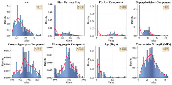
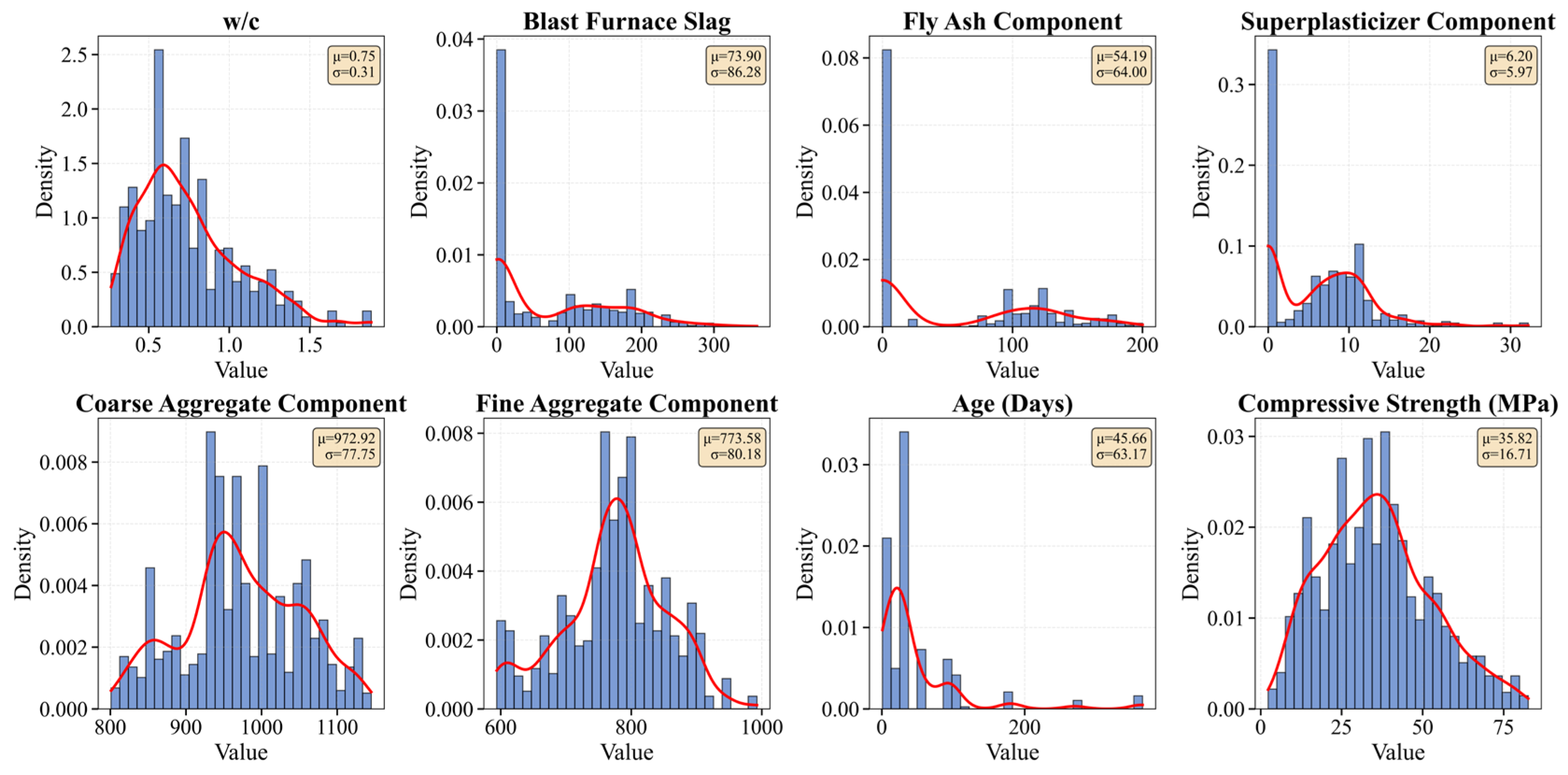
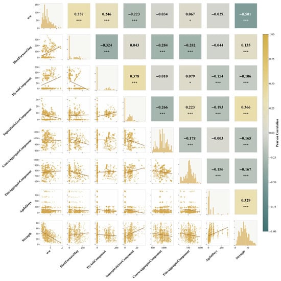
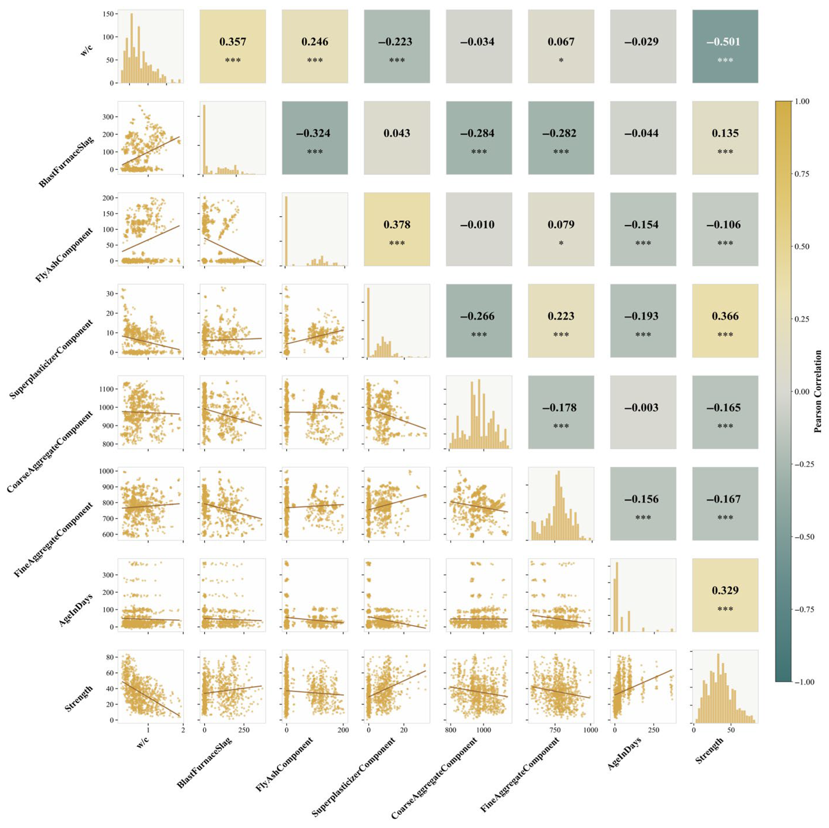
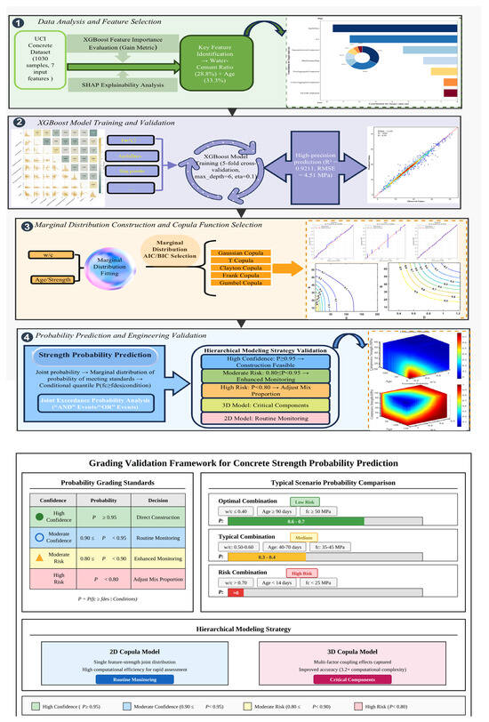
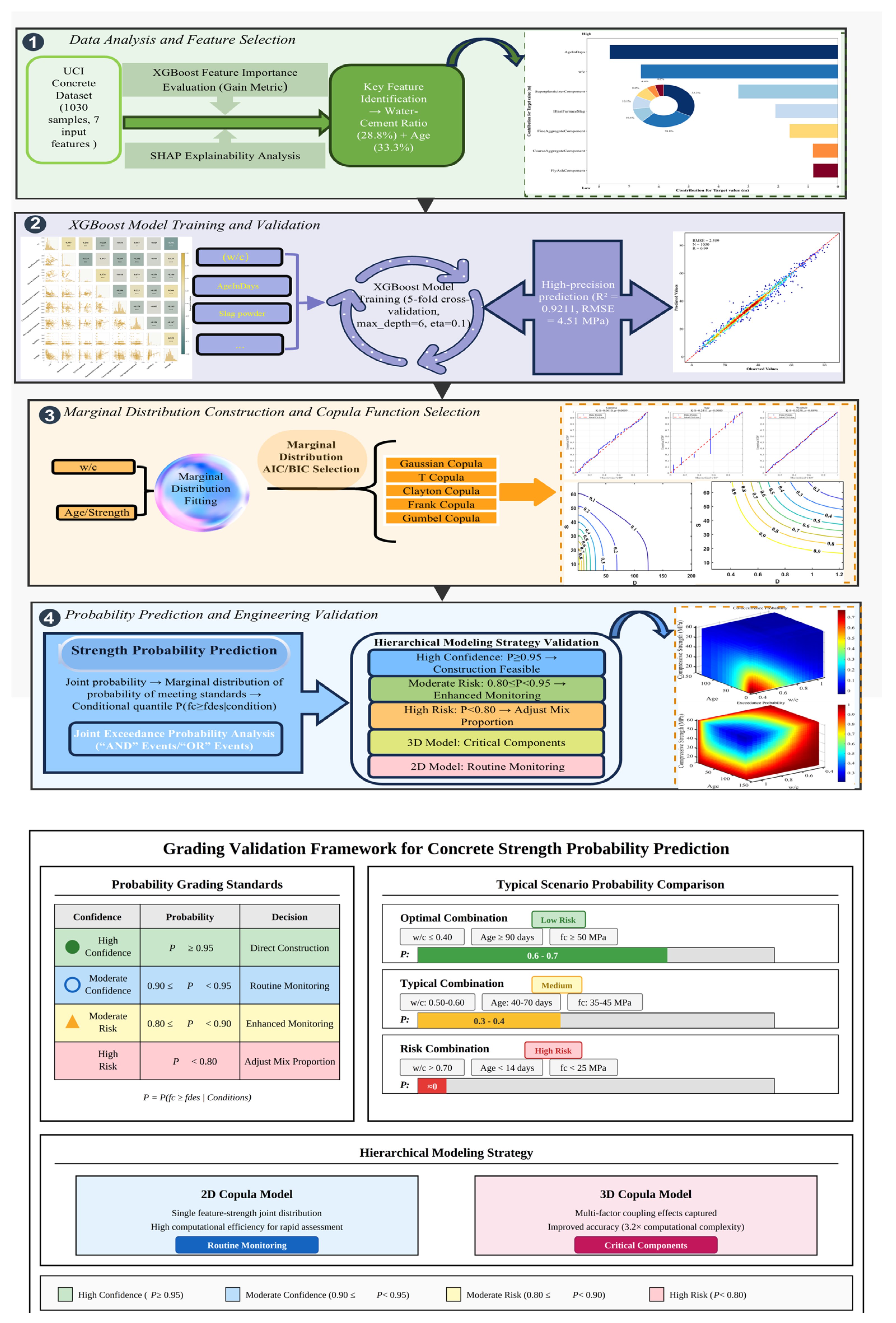
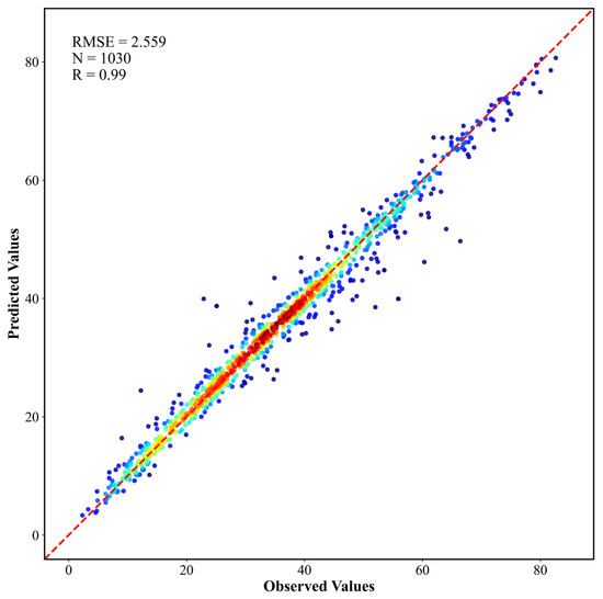
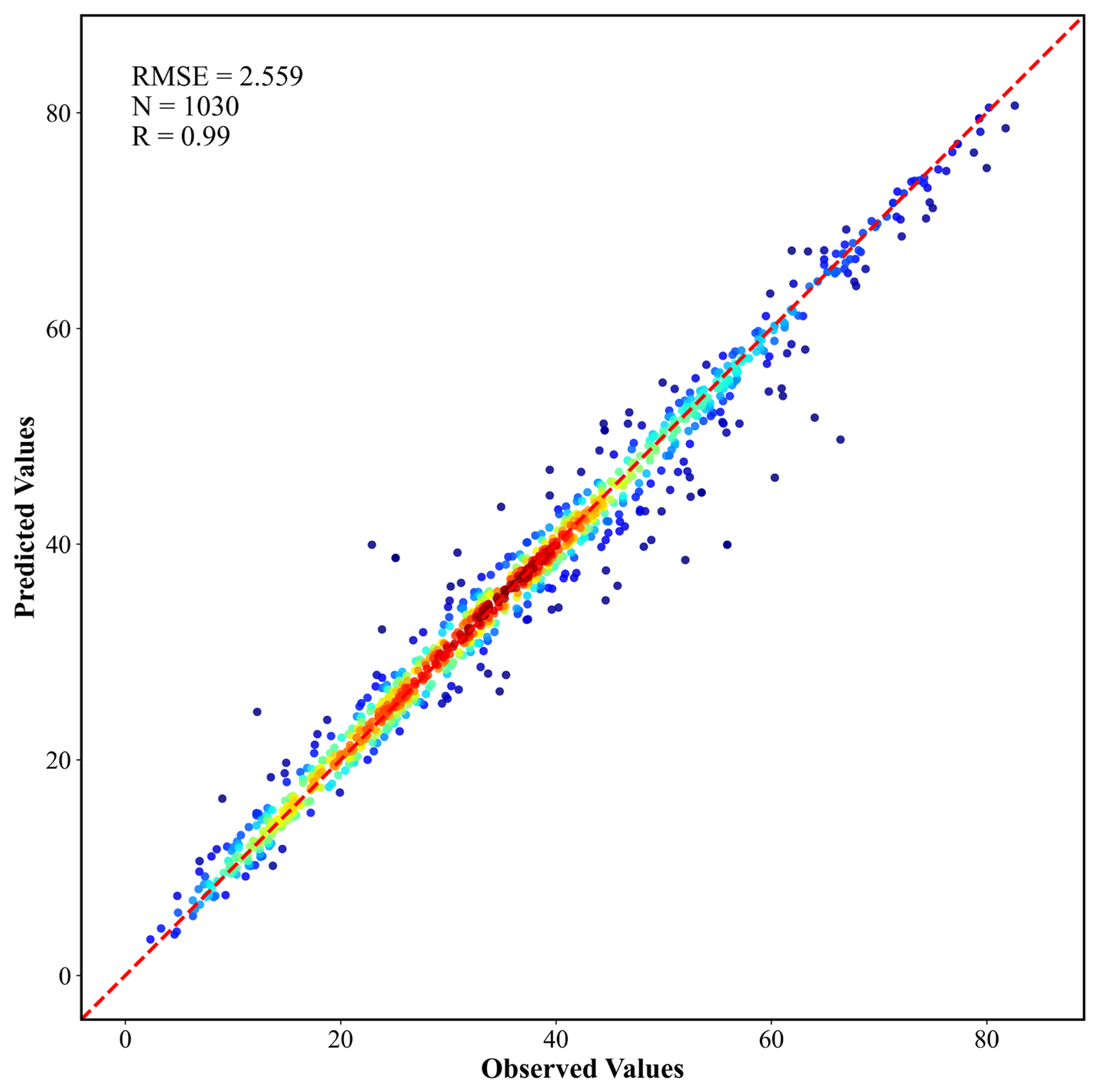
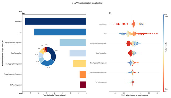
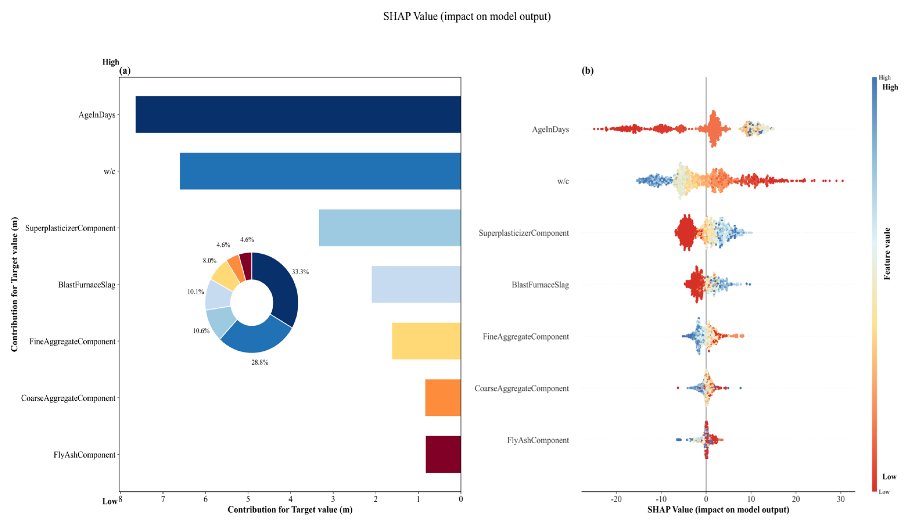
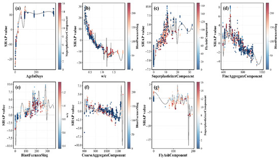
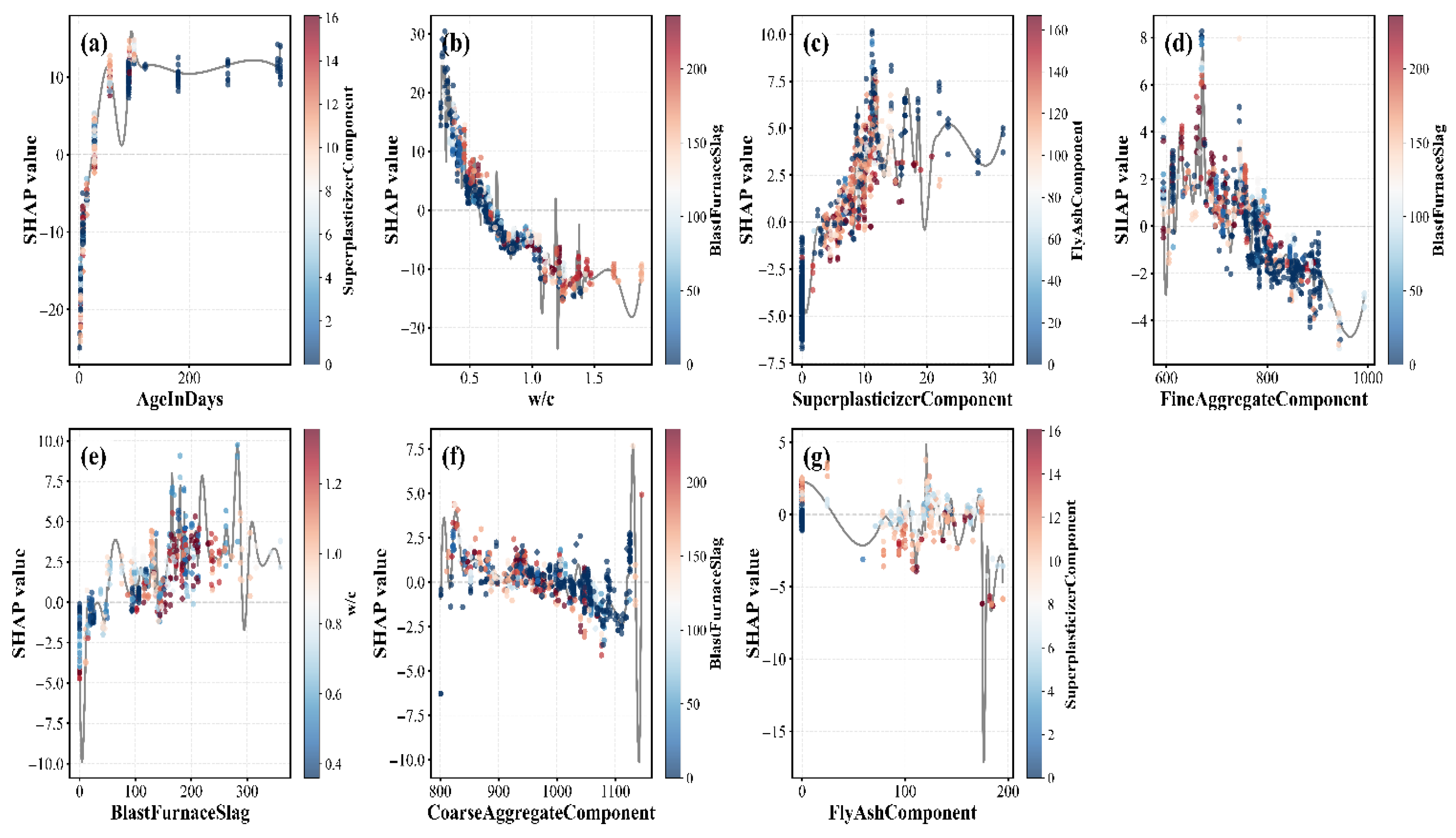
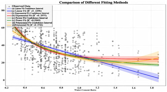
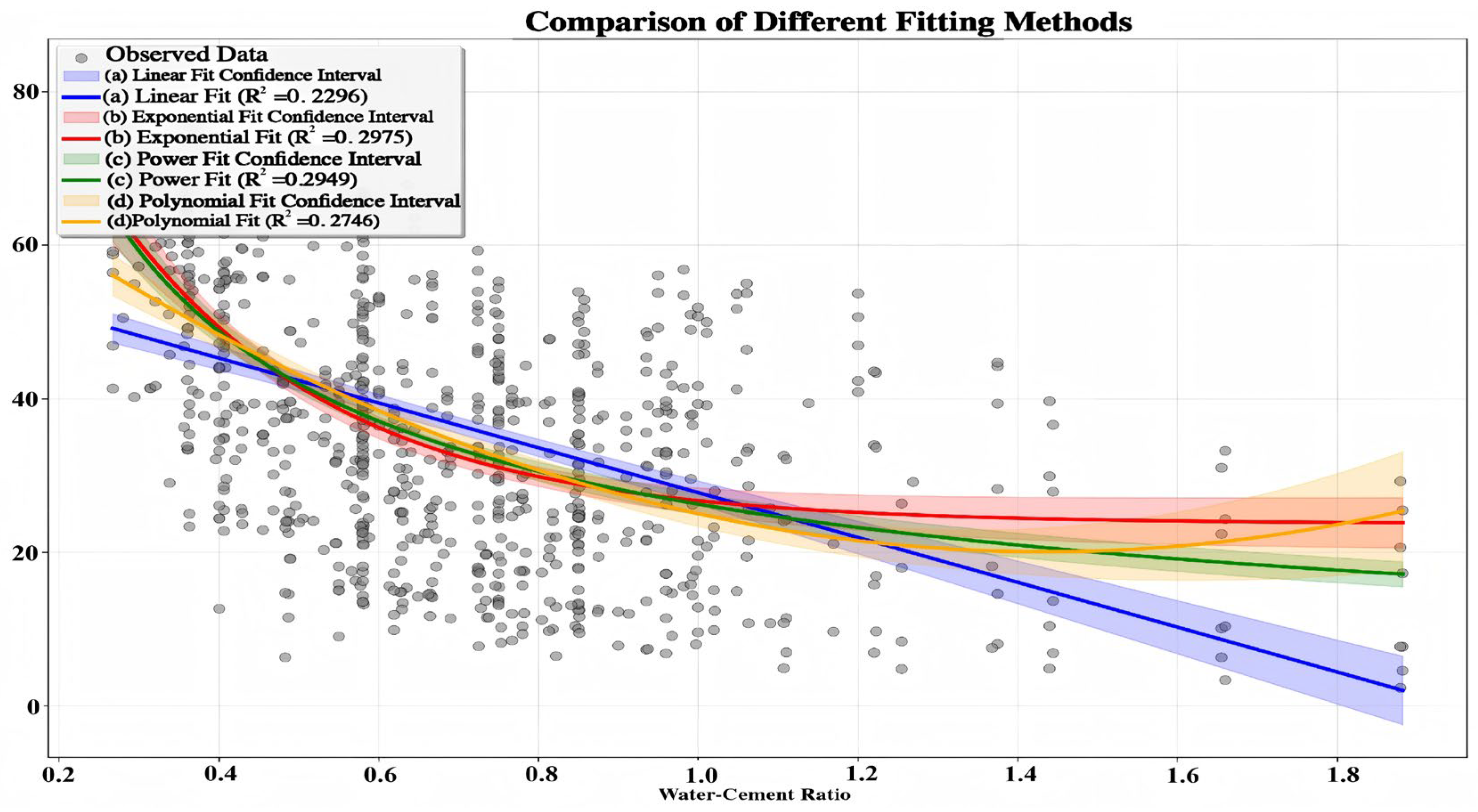
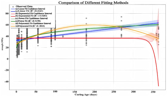
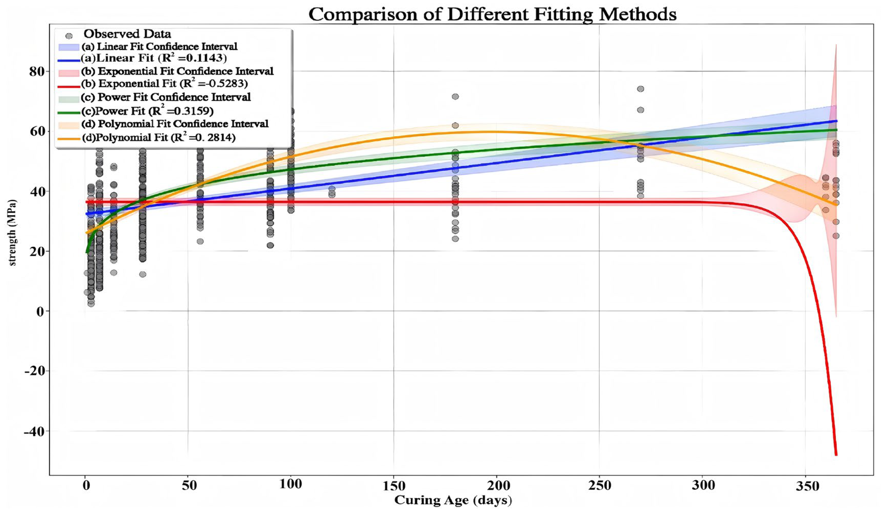
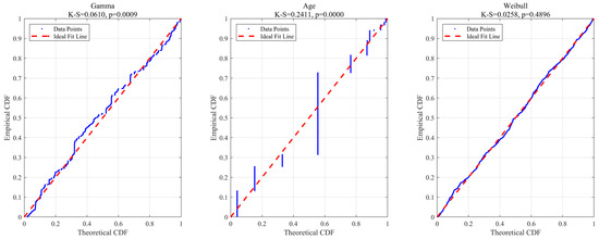
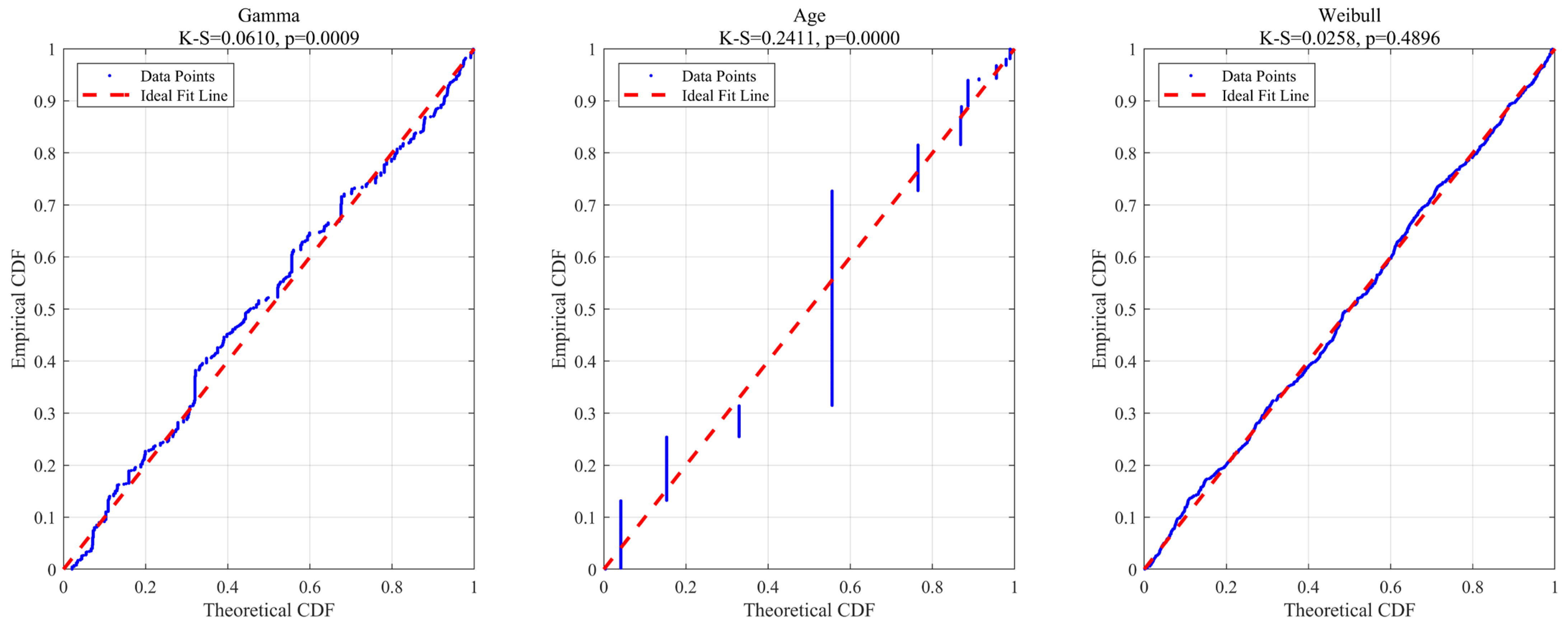
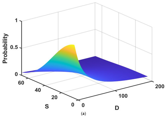
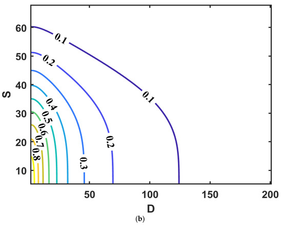
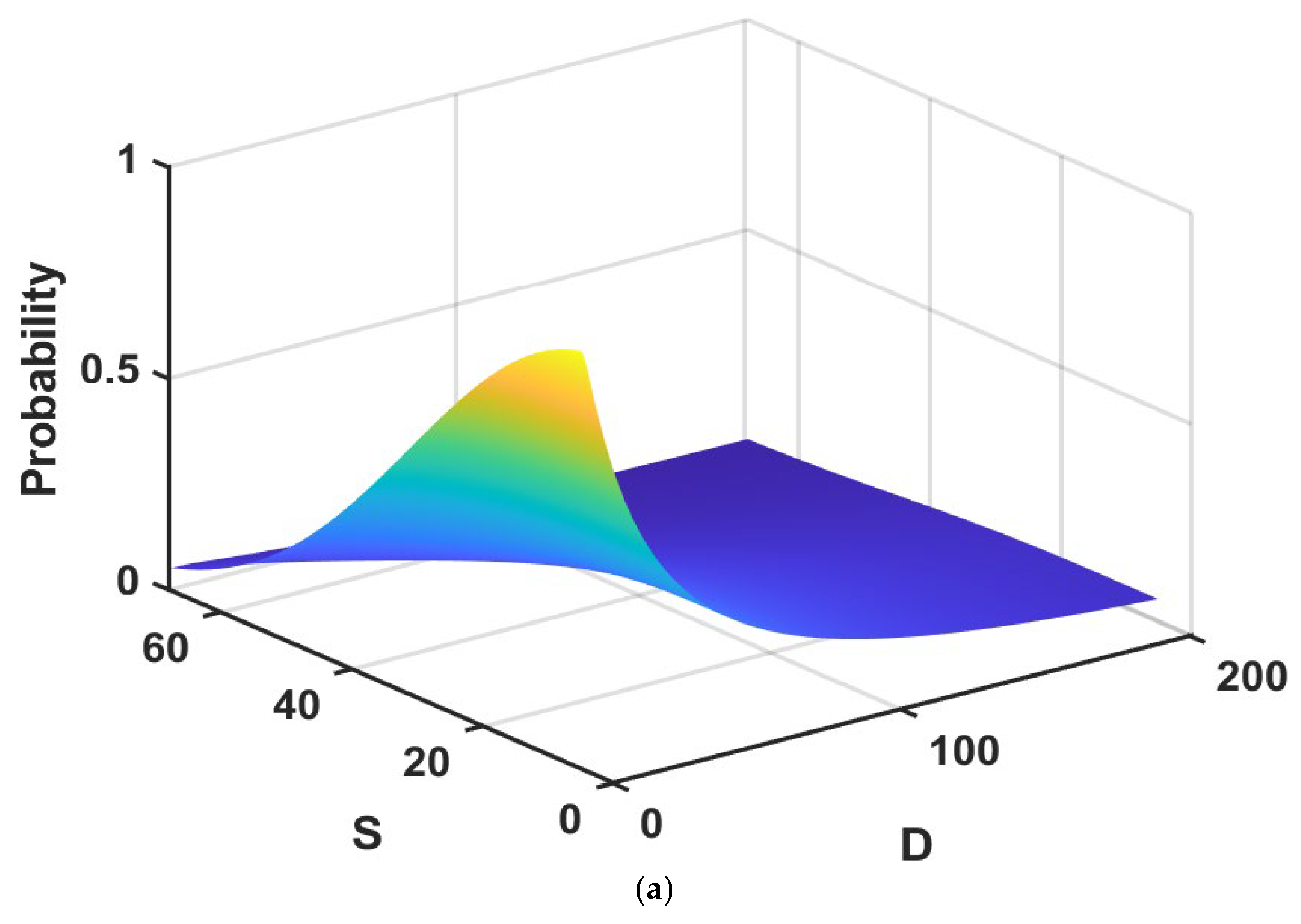
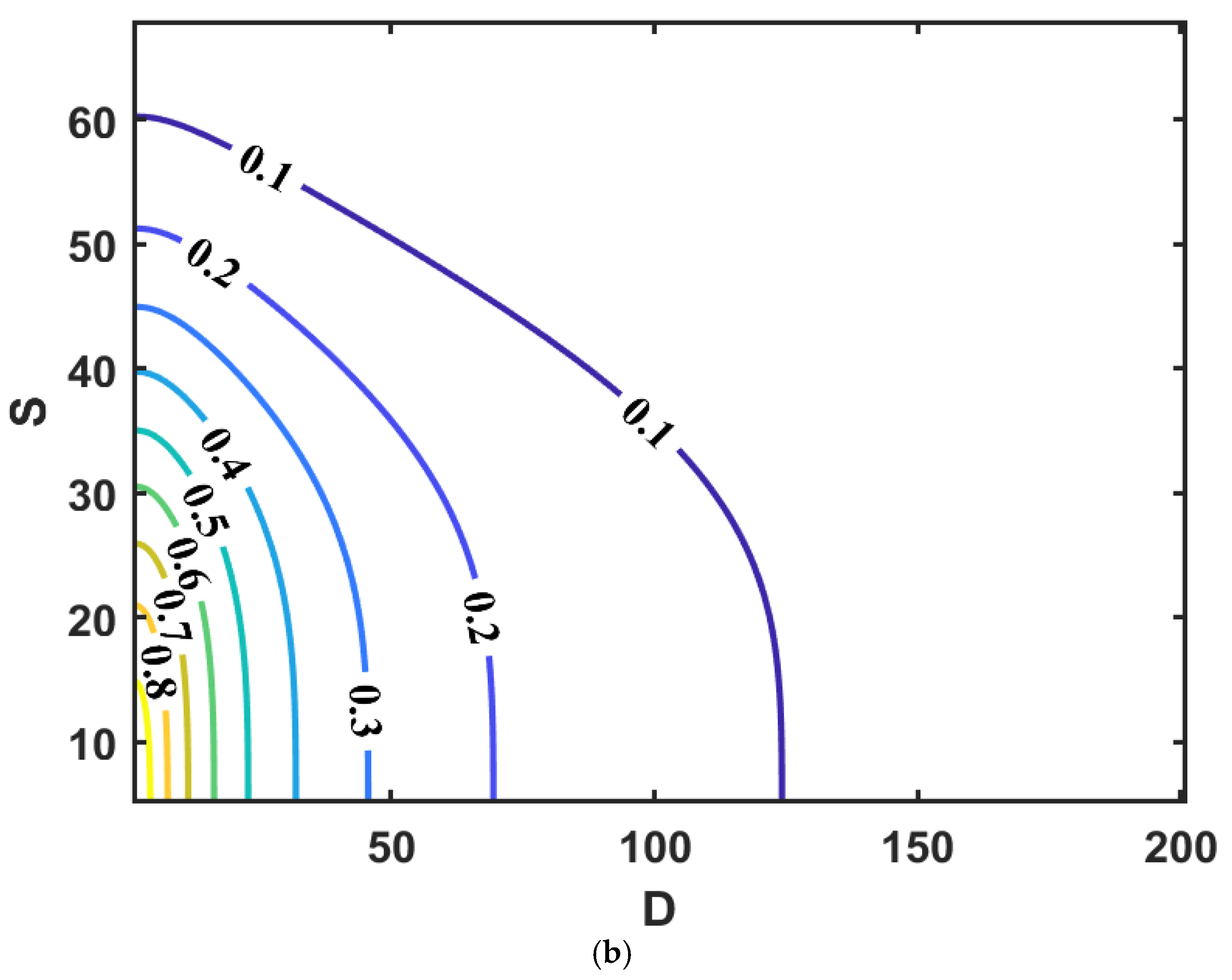
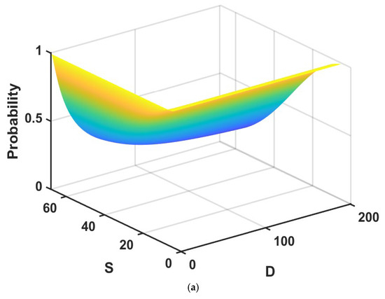
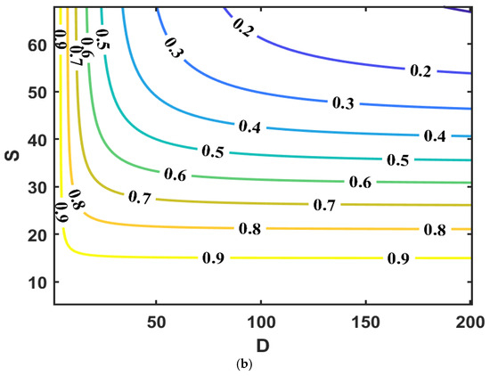
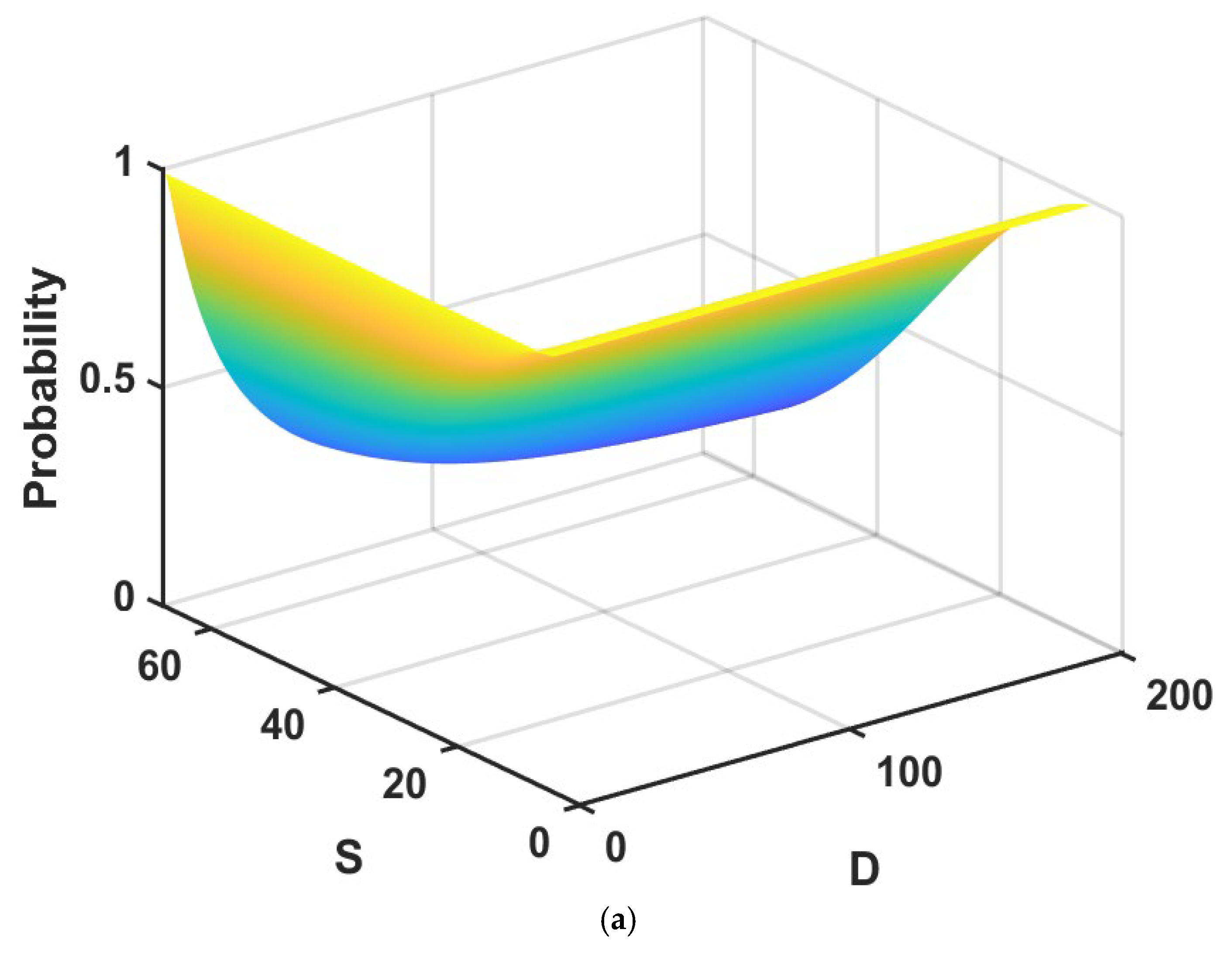
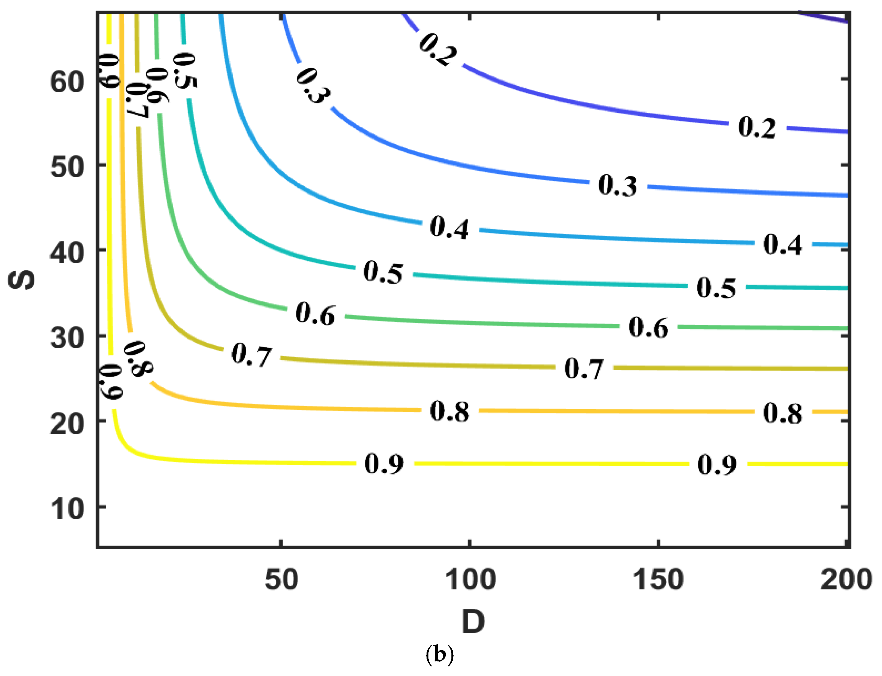
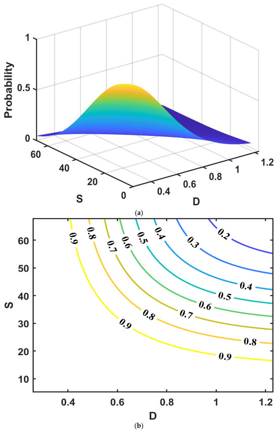
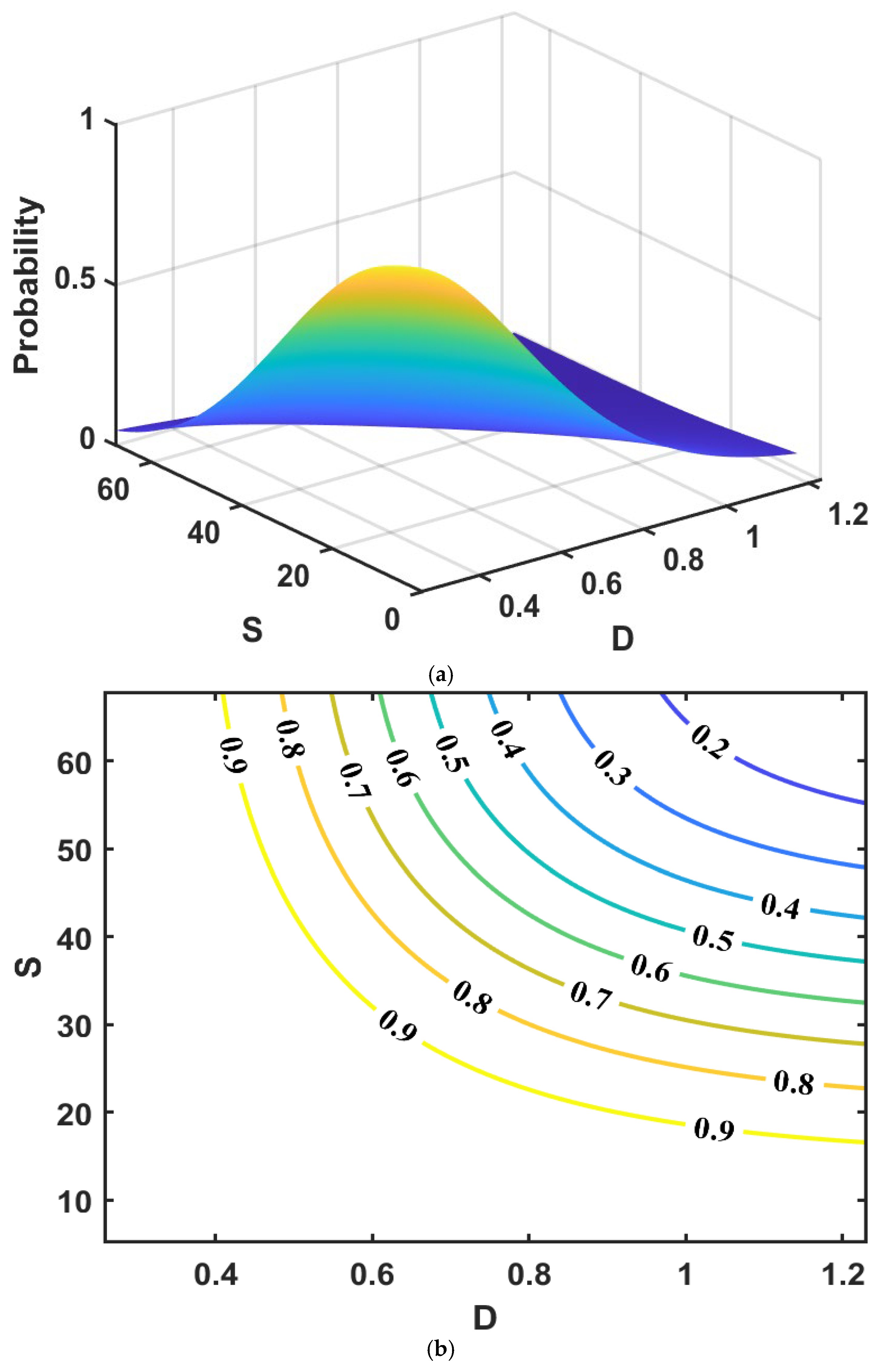
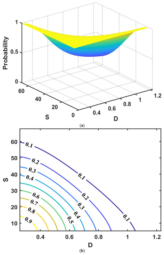
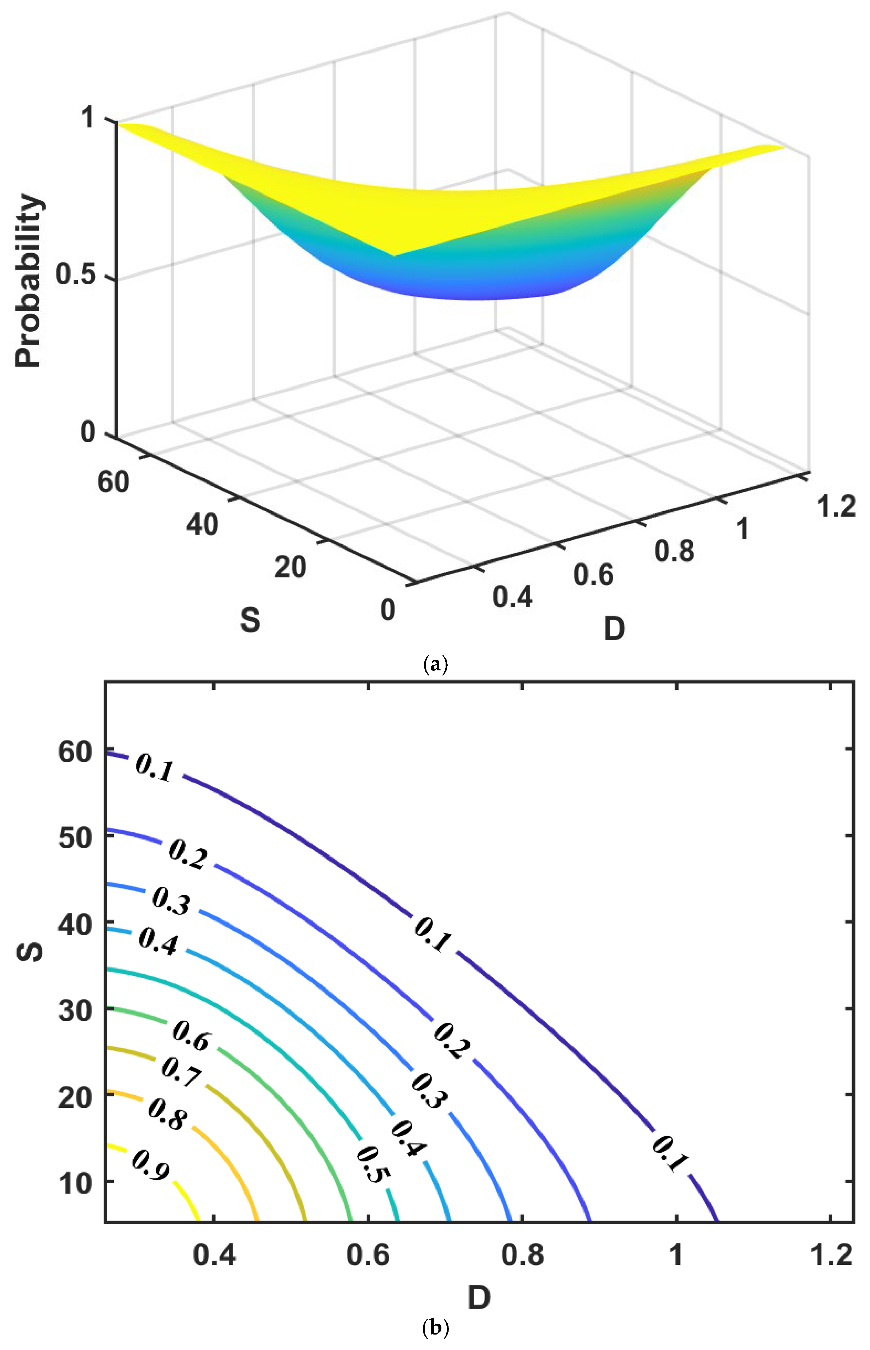
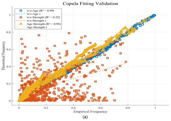
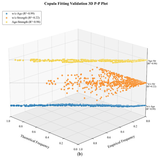
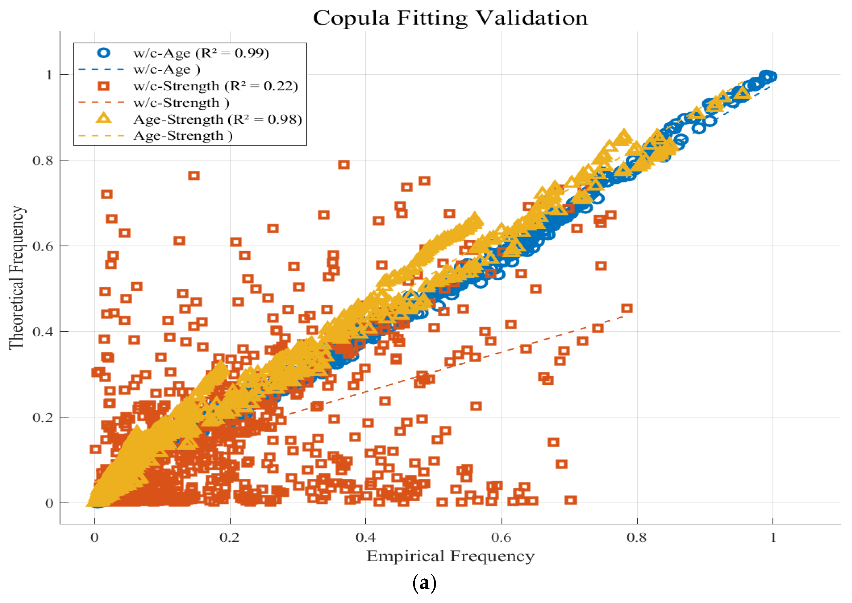
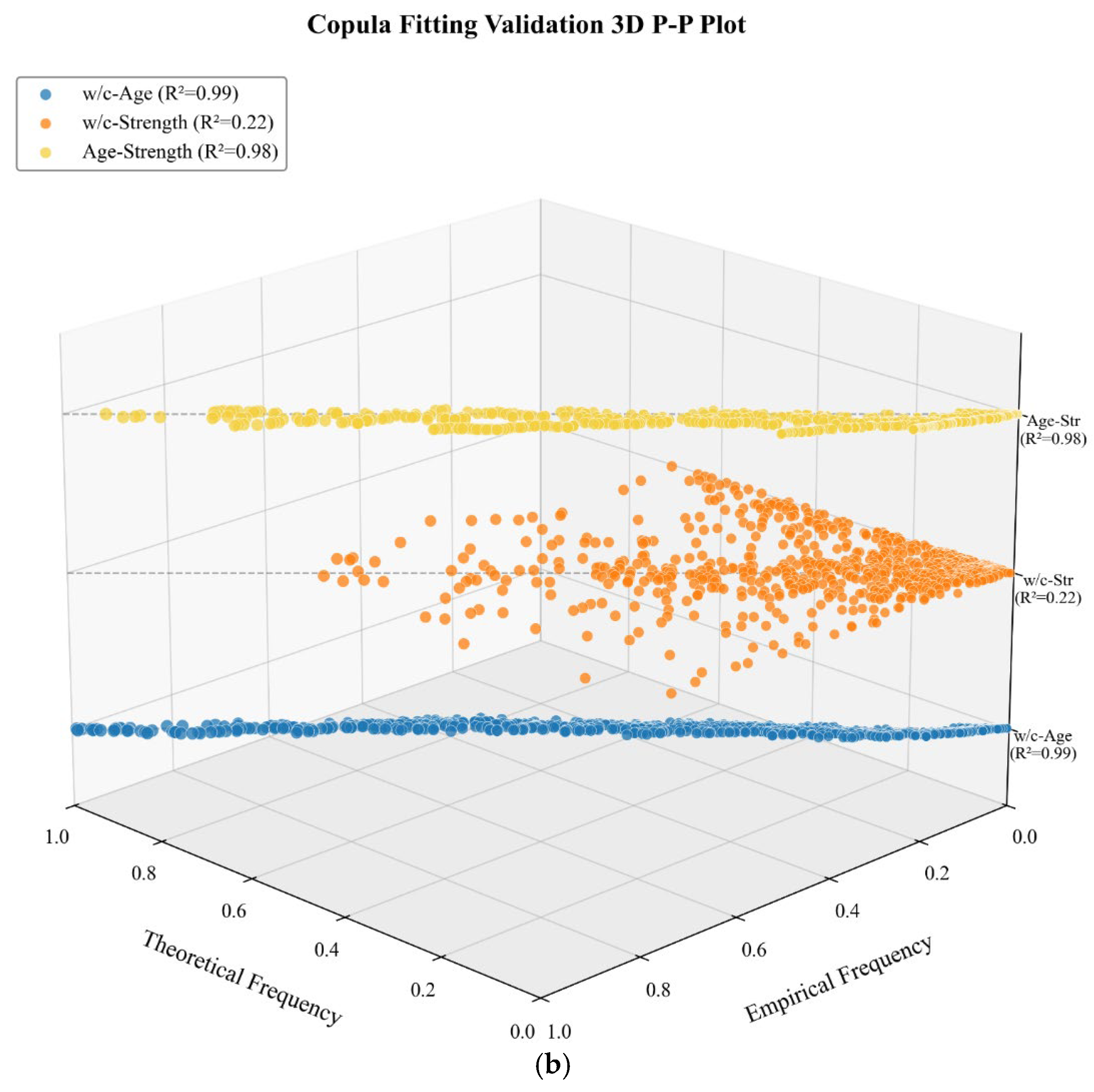
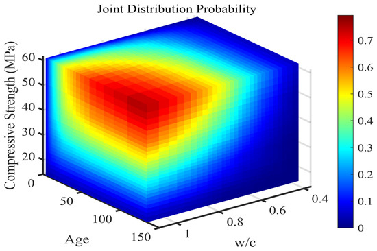
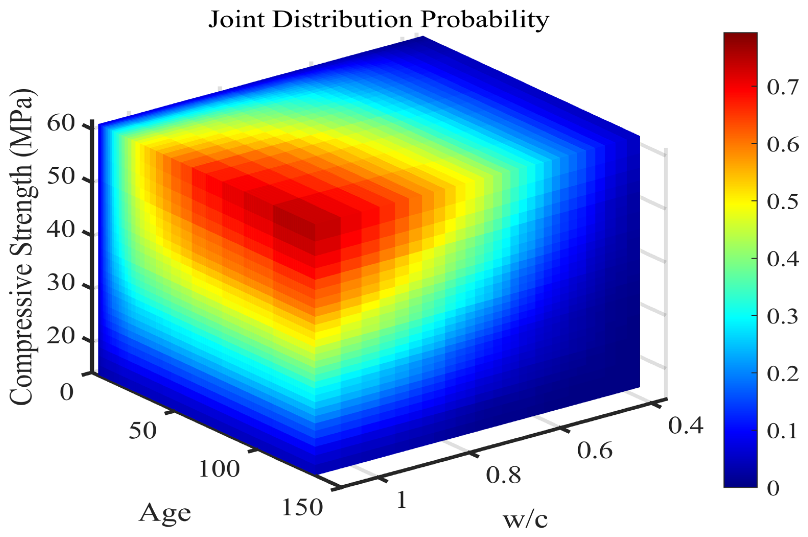
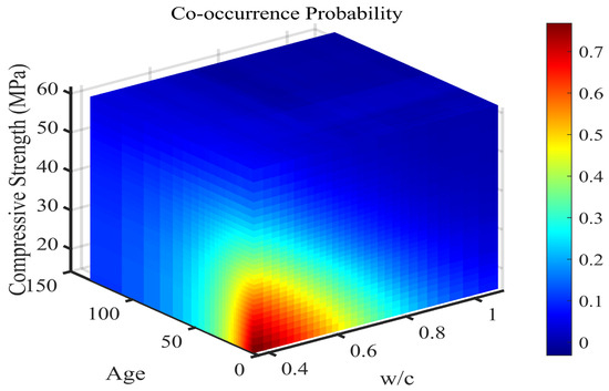
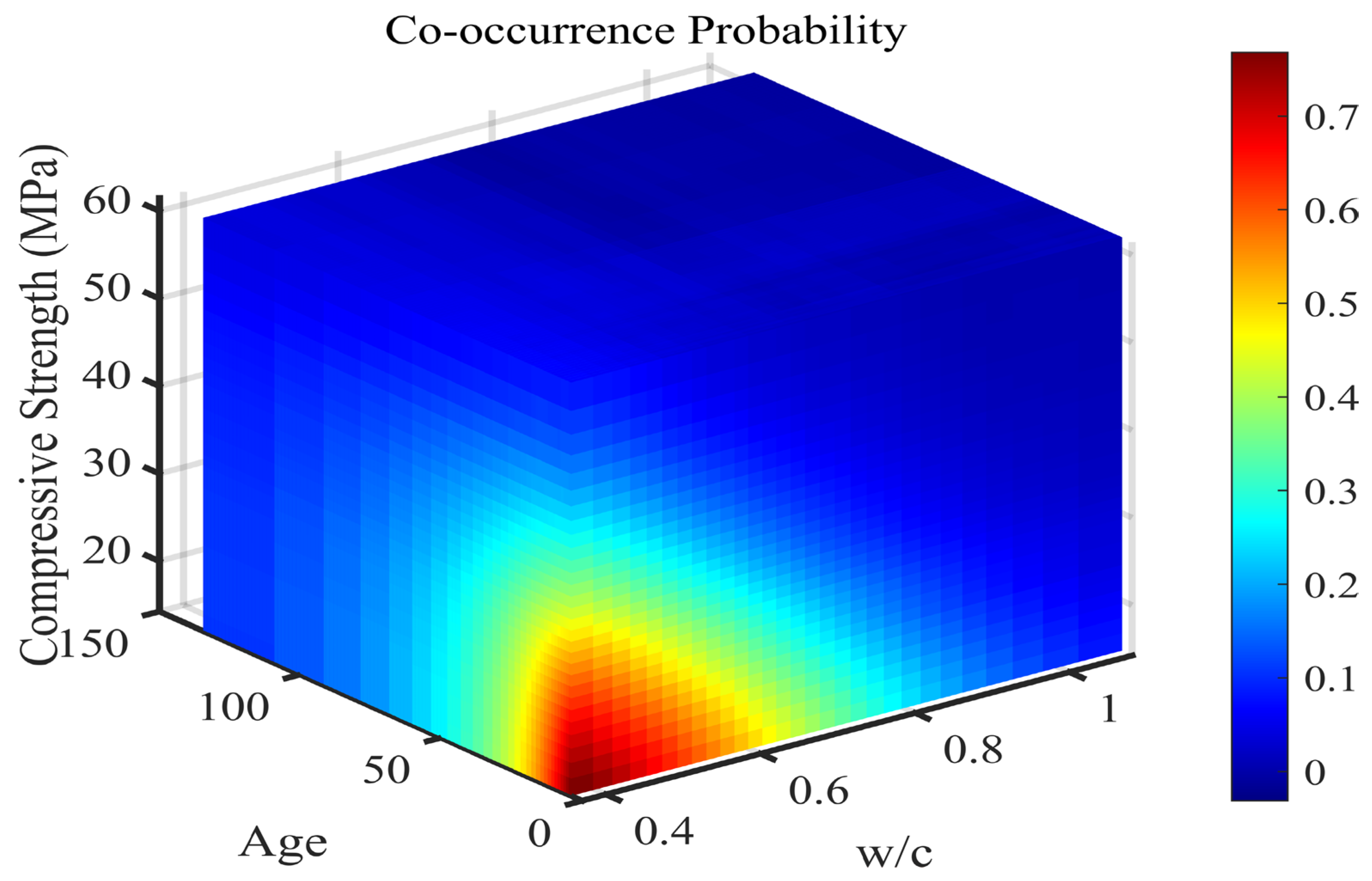
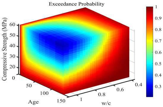
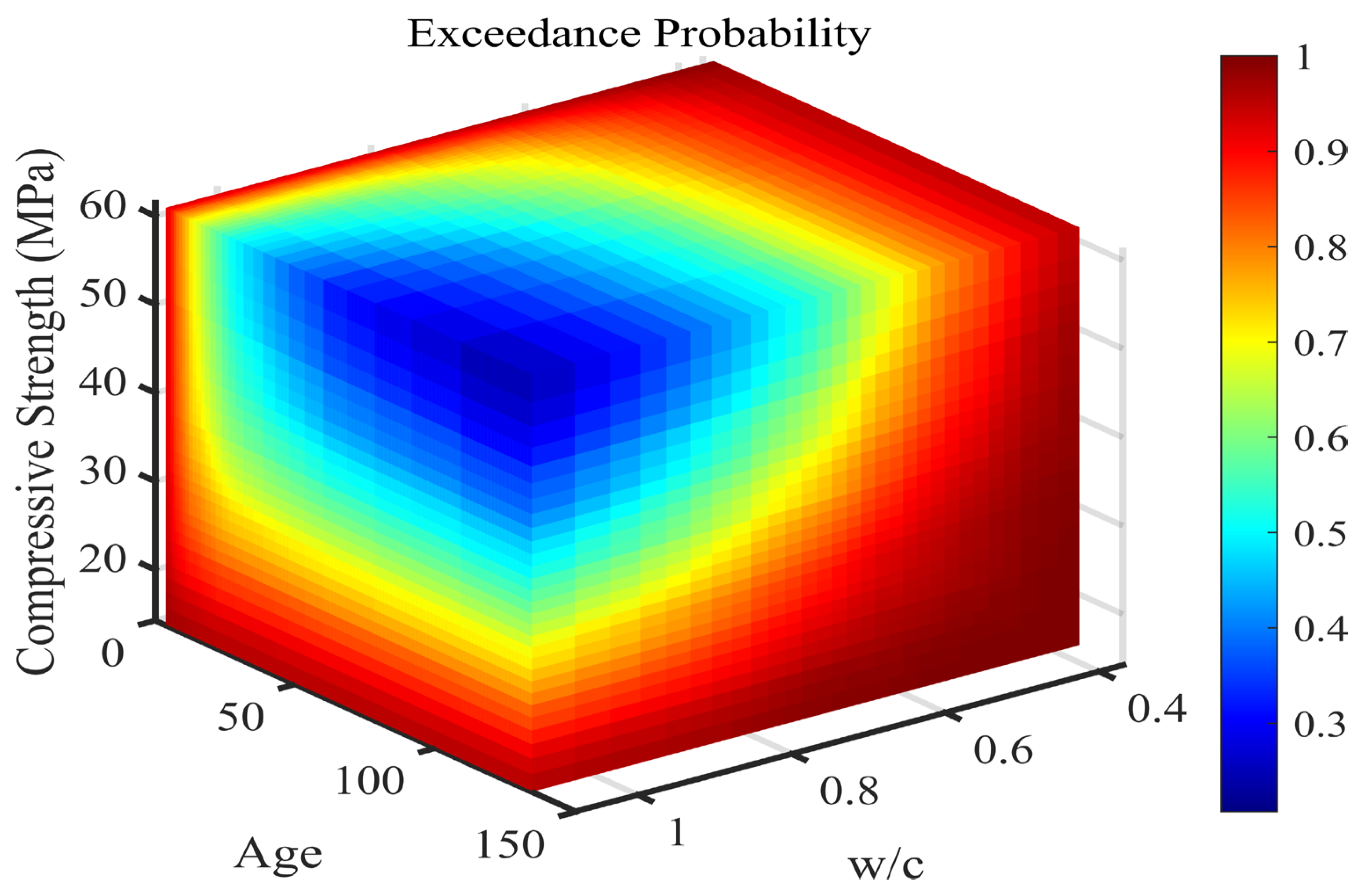
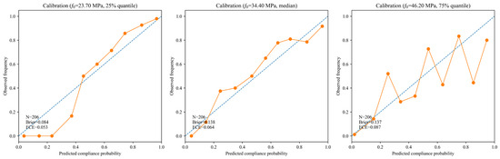
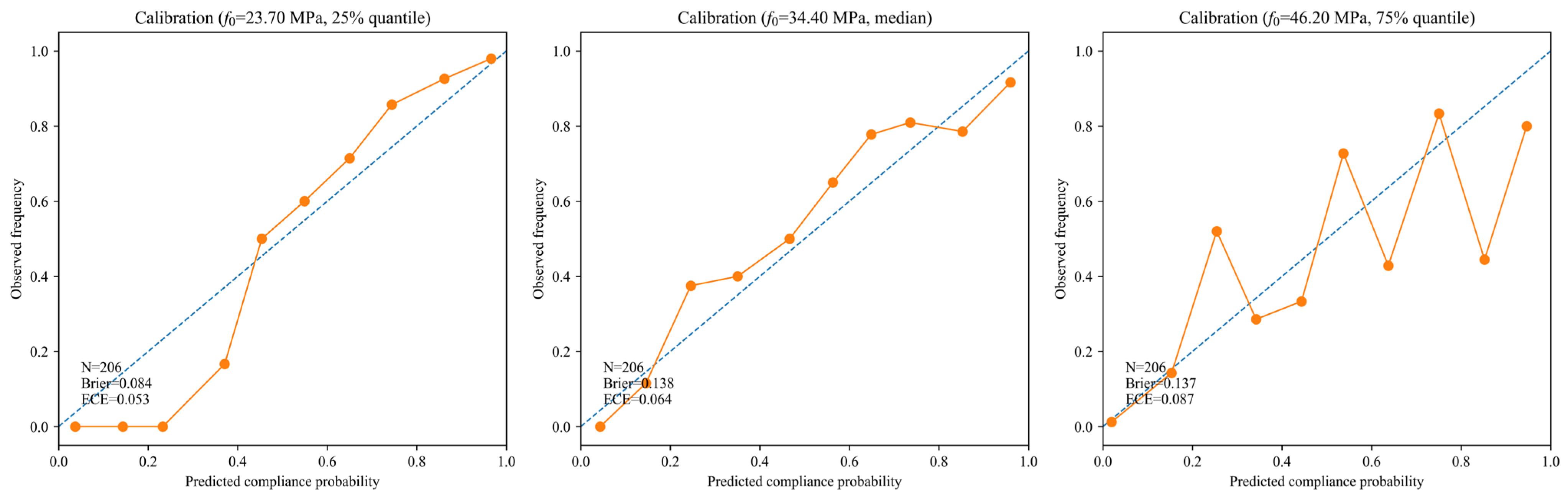
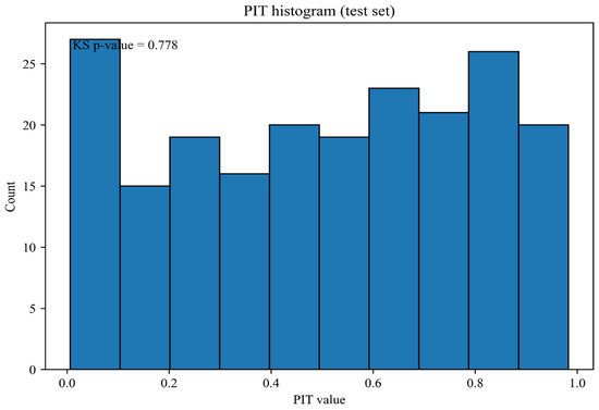
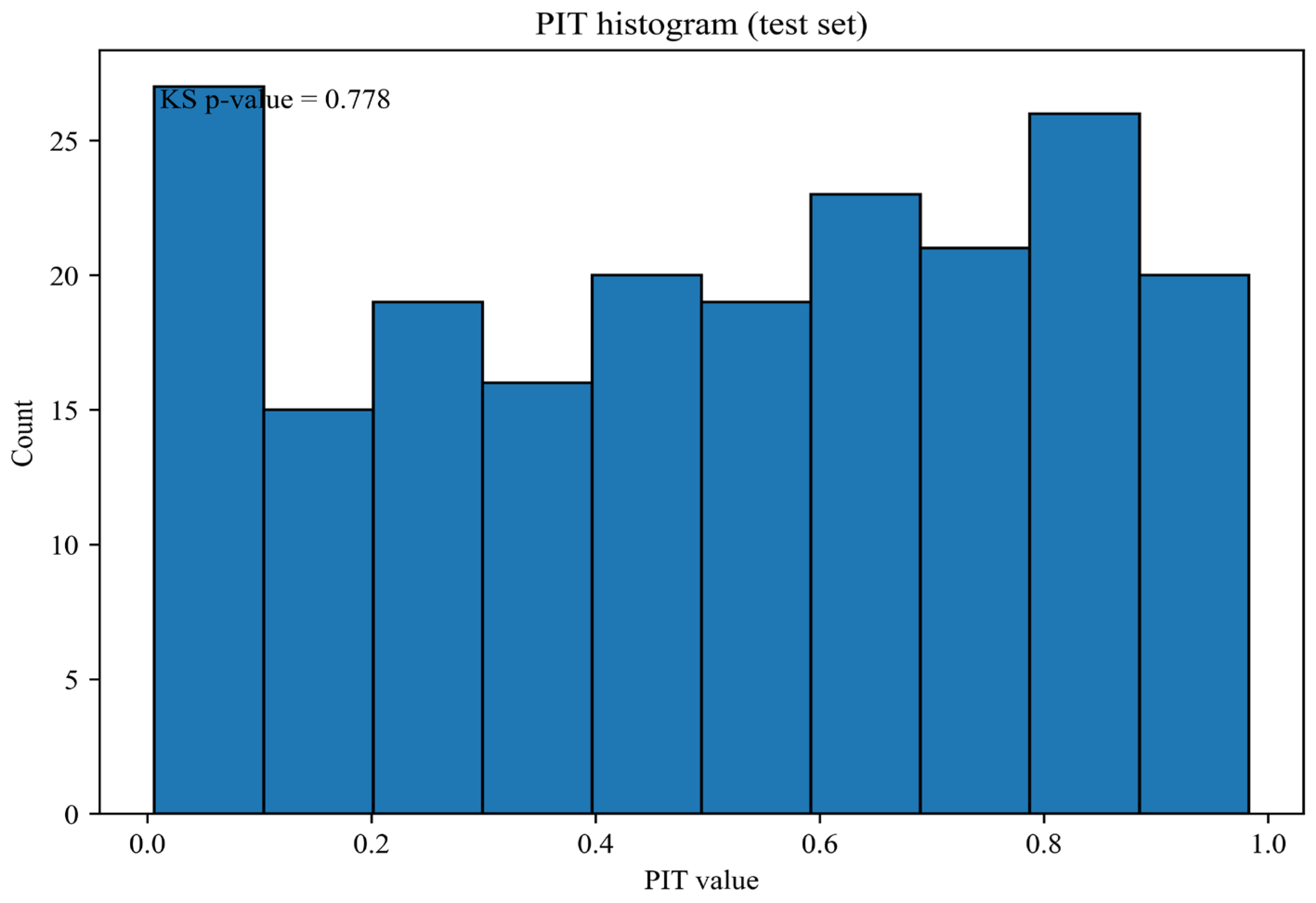

Disclaimer/Publisher’s Note: The statements, opinions and data contained in all publications are solely those of the individual author(s) and contributor(s) and not of MDPI and/or the editor(s). MDPI and/or the editor(s) disclaim responsibility for any injury to people or property resulting from any ideas, methods, instructions or products referred to in the content. |
© 2026 by the authors. Licensee MDPI, Basel, Switzerland. This article is an open access article distributed under the terms and conditions of the Creative Commons Attribution (CC BY) license.