


Abstract
Urban heat islands intensify heat exposure in high-density cities, but the nonlinear and spatially heterogeneous associations between urban morphology and daytime and nighttime urban heat island intensity (UHII) remain unclear. This study examines 4800 urban blocks within Beijing’s Fifth Ring Road by integrating Local Climate Zone (LCZ) classification, remote sensing observations, interpretable XGBoost, and geographically weighted machine learning. Relationships are assessed at citywide, LCZ-specific, and local scales. For the selected observation scenes, UHII was higher in built LCZ types than in land-cover types. Mean UHII was higher in the daytime scene using the LCZ B+D reference, but the ordering reversed with LCZ D alone. Daytime hotspots were spatially fragmented, whereas nighttime hotspots clustered in the urban core. The normalized difference vegetation index (NDVI) and impervious surface aggregation contributed most to daytime model predictions, with shifts in contribution direction near 0.43 and 0.96, respectively. Albedo and NDVI contributed most to nighttime predictions. Across LCZ types, NDVI remained important during the day; at night, building height dominated contributions in LCZ 1 and LCZ 3, while albedo dominated in LCZ 4 and LCZ 5. Geographically weighted modeling further identified local variation in morphological contributions. These findings identify LCZ-specific and local differences obscured by citywide summaries, providing evidence for spatially targeted heat mitigation and block-scale urban renewal.
1. Introduction
Global urbanization has continued to accelerate. According to the World Cities Report 2022, the share of the global population residing in urban areas is projected to increase from 56% in 2021 to 68% by 2050 [1]. The large-scale concentration of population and the continuous expansion of urban built-up areas have substantially intensified the urban heat island (UHI) [2,3,4]. UHI generally refers to a thermal anomaly whereby urban areas exhibit higher near-surface air temperatures or land surface temperatures (LST) than surrounding suburban areas, rural environments, or natural land surfaces [5]. The intensification of UHI deteriorates the urban thermal environment, reduces residents’ thermal comfort, increases heat-related health risks, and raises cooling energy demand during summer [6]. It may also promote the accumulation and secondary formation of air pollutants, such as ground-level ozone, thereby exerting adverse effects on urban ecological quality [7]. Notably, the UHI exhibits pronounced asymmetry between daytime and nighttime, with its formation mechanisms, spatial patterns, and health implications differing markedly. Compared with daytime heat exposure, which directly affects outdoor activities, transportation systems, and occupational safety, persistent nighttime heat is more likely to impede physiological recovery, weaken thermoregulatory capacity, and amplify heat-related health burdens [8]. Therefore, identifying the spatial differentiation of daytime and nighttime UHI intensity and elucidating their underlying driving mechanisms are essential for revealing the time-varying effects of urban morphological factors on the thermal environment. Such evidence can further provide a scientific basis for climate-adaptive urban planning and targeted thermal mitigation strategies.
The urban heat island (UHI) is commonly classified into daytime and nighttime UHI according to the time of day [9]. Existing studies have shown that daytime and nighttime UHI differ substantially in terms of thermal formation processes, spatial distribution patterns, and dominant influencing factors [9,10,11]. In terms of spatial patterns, daytime and nighttime UHI hotspots do not fully overlap [12]. Daytime UHI tends to exhibit a more fragmented and localized distribution, with high-temperature areas mainly concentrated in impervious surfaces with limited vegetation cover and insufficient shading. In contrast, nighttime UHI is more likely to form continuous thermal patterns in high-density built-up areas and often shows stronger spatial clustering [13]. Daytime and nighttime urban heat island intensity (UHII) is jointly affected by two-dimensional (2D) land-cover factors and three-dimensional (3D) urban morphological factors. However, the direction, magnitude, and relative importance of these factors differ markedly between daytime and nighttime periods [14,15,16]. During the day, shortwave solar radiation directly heats the land surface, making 2D land-cover factors, such as vegetation coverage, impervious surface fraction, albedo, and shading conditions, more directly associated with UHII [17]. Specifically, vegetation can reduce surface heat accumulation through evapotranspiration, shading, and reflection, whereas impervious surfaces with limited vegetation and shade are more prone to the formation of daytime heat islands [9,18]. At night, after the cessation of shortwave solar radiation, urban thermal processes shift from radiative heating to the release of stored heat. Heat accumulated during the day in land surfaces and building materials is gradually released into the urban canopy layer. During this process, 3D urban morphological factors, including building height, building density, sky view factor, building roughness, and canopy height, exert a more pronounced influence on nighttime UHII by regulating longwave radiation exchange, ventilation conditions, and heat storage and dissipation processes [14,15,16]. Moreover, the thermal effects of 3D urban morphology may exhibit asymmetric or even opposite responses between daytime and nighttime. During the day, building shadows can reduce solar radiation absorption by the land surface [19,20]. At night, however, a lower sky view factor may inhibit longwave radiation loss and enhance heat retention within dense urban spaces. Overall, existing research has recognized differences in the spatial patterns and driving factors of daytime and nighttime UHI. However, how the dominant thermal processes shift between daytime and nighttime in high-density built-up areas remains insufficiently explained. Therefore, it is necessary to introduce a classification framework capable of characterizing different urban morphological contexts, thereby providing a clearer basis for interpreting the differentiated effects of 2D land cover and 3D urban morphology on daytime and nighttime UHI.
The spatial heterogeneity of UHII is closely associated with variations in urban morphological contexts. If compact high-density built-up areas, low-density open areas, and areas with high green space coverage are analyzed within a single undifferentiated framework, the differences in the formation mechanisms of daytime and nighttime UHII across distinct morphological contexts may be obscured. The Local Climate Zone (LCZ) framework proposed by Stewart and Oke classifies urban space into typological units with relatively homogeneous morphological characteristics by standardizing land cover, urban structure, and human activity attributes [21]. The system comprises 17 standard classes, including 10 built types (LCZs 1–10) and seven land-cover types (LCZs A–G). Built types distinguish variations in building height, density, and arrangement, whereas land-cover types distinguish vegetation, bare surfaces, and water. For example, LCZ 1 represents compact high-rise development, while LCZ 4 represents open high-rise development. LCZs characterize relatively homogeneous areas at the local scale, typically extending from several hundred meters to several kilometers, providing a common basis for comparing thermal conditions across different landscapes [21]. This framework can help reduce interpretive bias in overall-sample analyses caused by the mixing of heterogeneous urban morphological contexts at the typological level. Previous studies have shown that the composite morphological characteristics represented by LCZ types affect heat storage, radiation balance, and air exchange processes, leading to inter-type differences in daytime warming, nighttime heat retention, and heat dissipation capacity [21,22]. These contextual differences may further influence both the dominant role and the effect intensity of urban morphological factors. For example, in compact built types, factors related to building coverage are more likely to produce a warming effect, whereas in LCZ 4, LCZ 5, and LCZ 6, which are characterized by lower building density and relatively higher green space coverage, the summer warming effect of the impervious surface aggregation index may be more pronounced [23]. However, although LCZs provide a typological classification of urban morphological contexts, block-scale morphological differences and local spatial variations may still exist within the same LCZ type. Compared with regular grids and administrative units, urban blocks are more closely aligned with the operational scale of urban planning and renewal interventions [24,25]. Therefore, introducing LCZ stratification at the block scale in this study can not only facilitate the comparison of daytime and nighttime UHII across distinct urban morphological contexts, but also provide an analytical basis for integrating nonlinear and spatially heterogeneous modeling methods to reveal the differentiated effects of urban morphological factors on daytime and nighttime UHII within different LCZ contexts.
Building on the LCZ classification framework, further identifying the nonlinear associations between urban morphological factors and daytime and nighttime UHII and their spatial heterogeneity is essential for understanding morphology–UHII relationships under different morphological contexts. In terms of modeling approaches, geographically weighted machine learning (GWML) provides a promising analytical pathway for this purpose. By constructing local machine learning models at different spatial locations and incorporating spatial weights to characterize neighborhood relationships among samples, GWML can identify nonlinear responses and variable contributions while revealing local variations in factor contributions across space. This approach has already been applied to the study of green-space configuration and urban heat mitigation [26]. For studies of daytime and nighttime UHII, GWML can complement the LCZ classification framework. Specifically, LCZs are used to distinguish different urban morphological contexts, whereas GWML further characterizes the continuous spatial heterogeneity of factor contributions within and across LCZ contexts. In contrast, traditional methods such as multiple linear regression and ordinary least squares have clear model structures and strong interpretability, but they generally rely on assumptions of linearity and spatial stationarity. As a result, they are often insufficient for capturing the nonlinear responses between urban morphological factors and UHII [27,28,29]. Machine learning methods, including random forest (RF), gradient boosting regression (GBR), and extreme gradient boosting (XGBoost), provide effective tools for identifying complex relationships, variable contributions, and nonlinear response patterns [30,31,32]. However, conventional machine learning models mainly reveal average relationships at the overall-sample level and remain limited in capturing spatial variations in factor contributions. Geographically weighted models, such as geographically weighted regression (GWR), can reveal spatial non-stationarity in variable relationships, but they are relatively constrained in modeling complex nonlinear responses [33,34]. Therefore, this study applies GWML within the LCZ-stratified analytical framework to simultaneously characterize nonlinear responses of daytime and nighttime UHII, differences in variable contributions, and local spatial heterogeneity. Studies of Beijing’s surface thermal environment have characterized diurnal surface urban heat island patterns across LCZs and examined their spatial determinants [35]. At the block scale, morphology-based classification combined with XGBoost and Shapley additive explanations (SHAP) has revealed nonlinear associations between urban form and land surface temperature [36]. Research on Beijing’s residential areas has examined nonlinear morphology–LST relationships at global and morphology-specific levels and spatial heterogeneity at the local level [37]. Building on these studies, the present work investigates how the relative importance and spatial patterns of morphological contributions vary across LCZ types and street blocks within Beijing’s Fifth Ring Road under the selected daytime and nighttime observation conditions.
Specifically, this study aims to: (1) Calculate UHII for the selected daytime and nighttime scenes at the block scale within the LCZ framework and analyze their spatial patterns across different LCZ types; (2) Construct a system of 2D and 3D urban morphological factors to identify the key factors associated with daytime and nighttime UHII at both the overall-sample and LCZ-stratified levels, and further analyze their relative contributions and nonlinear response characteristics; (3) Identify local spatial differences in the contributions of urban morphological factors using GWML, thereby complementing overall-sample and LCZ-stratified interpretations at the block scale.
2. Study Area and Data
2.1. Study Area
Beijing is located in North China (115.7–117.4° E, 39.4–41.6° N) and is a typical highly urbanized megacity in China (Figure 1). It has a warm-temperate, semi-humid continental monsoon climate, characterized by hot and rainy summers and cold and dry winters [38]. June to September are typically the hottest months of the year. In the Beijing Plain, persistent high temperatures, strong solar radiation, and extensive high-intensity urban surfaces jointly exacerbate daytime urban thermal environment problems. Previous studies have shown that Beijing’s surface UHI exhibits marked variation between daytime and nighttime, with daytime UHI being more pronounced in summer, whereas nighttime UHI is strongly influenced by heat storage and release processes in urban surfaces [39]. Given the high level of urban development, diverse block types, and strong demand for thermal environment regulation within Beijing’s Fifth Ring Road, this study focuses on urban blocks in this area. The study area covers approximately 668 km2 and includes 4800 urban blocks, encompassing a range of typical spatial types, such as the historic palace district (A), high-density commercial districts (B), traditional hutong urban blocks (C), and large-scale blue-green ecological spaces (D). It is one of the most highly urbanized areas in Beijing and contains some of the city’s most complex land surface types [40].
Figure 1.
Study area.
2.2. Dataset
The data used in this study were obtained from multiple publicly available datasets, with detailed sources and descriptions provided in Table 1. Urban block boundaries were obtained from the Multi-level Street-block Divisions of 985 Cities Worldwide (MSDCW) dataset [41]. These data served as the basic analytical units and provided the spatial framework for variable aggregation and spatial matching in subsequent analyses. LST data were obtained from the ECOSTRESS LST product provided by the NASA LP DAAC (https://www.earthdata.nasa.gov), with a spatial resolution of 70 m, to extract daytime and nighttime LST values for the study area. In addition, hourly LST products from the Copernicus Global Land Service (CGLS) were incorporated to correct for background thermal conditions in asynchronous ECOSTRESS imagery. Urban morphology data, including land cover, building, and canopy height datasets, were used to calculate 2D and 3D urban morphological factors. Land cover data were derived from GLC_FCS10 [42], building data from 3D-GloBFP [43] and canopy height data from sub-meter-resolution canopy height maps [44].
Table 1.
Details of the study data.
3. Methodology
3.1. Research Framework
This study consists of four main stages (Figure 2). First, multi-source data, including block-level data, Landsat 8 imagery, land cover data, building data, and tree height data, were integrated to provide the basis for subsequent LCZ classification and urban thermal environment analysis. Second, based on Landsat 8 imagery, machine learning methods were used to generate LCZ maps at a 30 m spatial resolution, which were further converted into block-scale LCZ classification results. Third, by integrating ECOSTRESS and CGLS LST products and applying image preprocessing and background thermal correction, daytime and nighttime UHII values were calculated, and 2D and 3D urban morphological factors were extracted. Finally, with urban morphological factors as independent variables and UHII as the dependent variable, the XGBoost-SHAP model was employed to analyze nonlinear relationships at both the overall-sample and LCZ-stratified levels. In addition, the GWML framework was used to identify local spatial heterogeneity in the relationships between urban morphological factors and UHII.
Figure 2.
Research and technological framework.
3.2. Machine Learning-Based LCZ Classification
Existing LCZ classification methods can generally be divided into three categories. The first category is manual annotation based on existing LCZ maps or standard LCZ frameworks, which is commonly used to compare urban thermal environments across different urban morphological units [45]. The second category is rule-based classification using geographic information systems and urban morphological parameters, in which LCZ types are identified according to indicators such as building height, sky view factor, and impervious surface aggregation index [46]. The third category is automated classification based on remote sensing imagery and machine learning, which uses multi-source Earth observation data and supervised classifiers for large-scale LCZ mapping [47]. This study adopts a machine learning-based LCZ classification method because it can integrate spectral, index-based, and topographic features from remote sensing imagery. Specifically, an LCZ classification workflow was established on the Google Earth Engine (GEE) platform. First, Landsat surface reflectance products were retrieved, and clouds, cloud shadows, and saturated pixels were masked to generate a median composite image for the target year. Second, indices including the normalized difference vegetation index, land surface water index, normalized difference built-up index, and modified normalized difference water index were calculated. These indices were then combined with the Shuttle Radar Topography Mission Digital Elevation Model (SRTM DEM), slope, and aspect to construct the classification feature set. Finally, manually interpreted LCZ samples were imported and divided into training and testing sets. The validation set contained 960 reference samples covering 14 LCZ classes. An RF classifier was used for LCZ classification, and a confusion matrix was constructed based on independent validation samples. Classification accuracy was assessed using overall accuracy, Kappa, and class-specific metrics (Table S14a,b). Subsequently, with urban blocks as the statistical units, the modal value of the 30 m LCZ raster within each block was extracted and assigned as the corresponding block-scale LCZ type. Table S13a summarizes the image scenes and quality-screening procedures.
3.3. LST Correction and UHII Calculation
This study used the ECOSTRESS LST product to obtain daytime and nighttime LST data for the study area and further calculate UHII. ECOSTRESS is a thermal infrared remote sensing mission aboard the International Space Station that provides multi-temporal LST observations at a spatial resolution of 70 m. In this study, ECOSTRESS images were selected based on a comprehensive evaluation of spatial coverage, valid-pixel integrity, data quality, and overpass time. The daytime scene was acquired at 14:30 on 15 June 2023 and the nighttime scene at 01:56 on 1 May 2023, both in Beijing time (UTC+8). This study compares urban thermal patterns and their associations with urban morphology under the selected daytime and nighttime observation conditions. Because the two scenes were acquired on different dates, the observed contrasts may reflect both diurnal processes and date-dependent environmental conditions. The purpose of the CGLS-based adjustment is to estimate the departure of LST at each location and observation time from the corresponding reference-period mean and to apply an additive adjustment to ECOSTRESS LST [48]. Specifically, for each ECOSTRESS observation scene and location, the additive CGLS-based adjustment was defined as the mean CGLS LST at the corresponding observation time over the reference period minus the CGLS LST matched to the ECOSTRESS acquisition date and time:
Here, denotes a pixel location on the ECOSTRESS grid, and denotes the selected daytime or nighttime observation scene. and represent ECOSTRESS LST before and after the CGLS-based adjustment, respectively. The terms and denote the acquisition date and time of scene , with acquisition times expressed in UTC for matching with CGLS data. The corresponding UTC dates and times are 15 June 2023 at 06:30 for the daytime scene and 30 April 2023 at 17:56 for the nighttime scene. denotes the reference period used to calculate the mean CGLS LST at the corresponding observation time. represents the mean of valid CGLS LST observations at the corresponding time over , whereas denotes the CGLS LST corresponding to the ECOSTRESS acquisition date and observation time. Both CGLS terms refer to values spatially aligned with the ECOSTRESS grid. Temperatures are expressed in °C, and is an additive temperature adjustment expressed in °C. CGLS fields were spatially aligned with each ECOSTRESS scene using bilinear resampling. The adjustment was applied at the pixel level before block-level aggregation. After adjustment, the 70 m ECOSTRESS LST raster was aggregated to the block scale using mean aggregation to obtain the block-average LST.
LCZ B (scattered trees) and LCZ D (low plants) were selected to define an internal vegetated thermal reference within the study area. Previous studies have used LCZ B as a thermal reference or explicitly evaluated it among alternative reference definitions [49,50,51], while LCZ D has also been used as the reference class in LCZ-based surface heat island analyses [35,52,53]. In this study, combining B and D provides an internal baseline representing both scattered-tree and low-plant cover. For each scene, the internal vegetated reference temperature was calculated by summing the adjusted block-average LSTs of all reference blocks classified as LCZ B or LCZ D and dividing this sum by the total number of these reference blocks. Each reference block was assigned equal weight. Block-level UHII (°C) was calculated by subtracting this reference temperature from the adjusted mean LST of each block. UHII here denotes a within-city surface thermal anomaly relative to an internal vegetated reference. At the block scale, UHII was calculated as follows:
where denotes the UHII of block , and denotes its mean land surface temperature. and are the sets of reference blocks classified as LCZ B and LCZ D, respectively, and and are their respective numbers. Sensitivity to the original CGLS processing was assessed by comparing mean LST and mean UHII with and without the processing for the same 4800 blocks in each scene (Table S6). Sensitivity of the top five predictor rankings to CGLS processing was assessed through model reruns (Table S7). Figure S2 provides a worked example of the calculation from adjusted pixel-level LST to block-level UHII.
3.4. Calculation of Urban Morphological Factors
This study selected 16 independent variables to characterize urban morphology at the block scale. These variables were classified into 2D and 3D urban morphological factors according to their attributes. The 2D urban morphological factors were mainly used to describe land-cover composition and planimetric spatial patterns within urban blocks, including the impervious surface aggregation index (AI_I), normalized difference vegetation index (NDVI), blue and green coverage ratio (BGCR), impervious surface landscape shape index (LSI_I), building density (BD), albedo (ALB), aggregation index of green spaces (AI_G), and green space landscape shape index (LSI_G). The 3D urban morphological factors were used to characterize the vertical structure, spatial configuration, and volumetric properties of buildings and vegetation, including building height (BH), building height variability (NHV), sky view factor (SVF), tree height (TH), distribution evenness index (DEI), building shape coefficient (BSC), mean building volume (MBV), and building volume density (BVD). The definitions and calculation methods of these factors are provided in Table 2. BH used footprint-area weights, DEI used footprint-to-block-area ratios, and NHV and MBV weighted buildings equally. Valid structural zeros were retained, whereas blocks lacking a valid observation for any predictor were excluded from modeling. Of the 6436 blocks, 1636 (25.42%) were excluded, leaving 4800 blocks for each of the daytime and nighttime analyses. Table S11 summarizes the observed range of each predictor before sample exclusion, including valid zeros.
Table 2.
Urban morphological factors and their calculation methods.
3.5. Interpretable Machine Learning Model
In the main analysis, the XGBoost and GW-XGBoost fits used predictor values on their stored input scales. This study introduces machine learning methods to characterize the response relationships between urban morphological factors and daytime and nighttime UHII. To assess the potential influence of multicollinearity among explanatory variables on model interpretation, variance inflation factor (VIF) tests were first conducted for all urban morphological factors. Compared with traditional models that assume a fixed functional form, machine learning methods can capture nonlinear responses, threshold effects, and variable interactions between urban morphological factors and UHII within a data-driven framework. These methods have been widely applied in the prediction and interpretation of urban thermal environments [54,55,56]. Accordingly, this study employs an XGBoost regression model to examine associations between urban morphological factors and UHII at both the overall-sample and LCZ-stratified levels, thereby providing the modeling basis for subsequent SHAP interpretation. The machine learning regression process can be summarized as follows:
where denotes the UHII of sample ; denotes the vector of urban morphological explanatory variables corresponding to sample ; denotes the model-predicted UHII for sample ; denotes the candidate function space; denotes the model complexity penalty term; and denotes the regularization coefficient. Standard five-fold cross-validation, with five equal folds of 960 blocks each, was used for model training, hyperparameter optimization, and performance evaluation in the main analysis. In each iteration, four folds were used for model fitting, and the remaining fold was used for validation. Root mean square error (RMSE) was used as the optimization objective, and the final model performance was reported as the average across the five validation folds. The model performance is provided in Table S2a, and the optimized parameters are provided in Table S3.
To further characterize local spatial variations in the relationships between urban morphological factors and UHII in the selected daytime and nighttime scenes, this study constructs a GWML framework. Using the same response variable and urban morphological predictors as the global models, GWML additionally incorporates sample coordinates to calculate spatial weights and fit a local model at each prediction location. Specifically, this study first uses the Haversine formula to calculate the spherical distance between sample points, then determines the neighboring sample set according to the local bandwidth, and finally calculates spatial weights using the bi-square kernel function:
where represents the weight assigned to training sample in the local model at location ; denotes the spatial distance between samples and ; denotes the local bandwidth; and is a small constant used to prevent the denominator from becoming zero. Samples closer to the prediction location are assigned higher weights, whereas samples outside the local bandwidth are assigned a weight of 0. Using this weighting scheme, we fitted geographically weighted XGBoost (GW-XGBoost) models to examine how the contributions of urban morphological factors to predicted UHII varied across street blocks in each observation scene. Bandwidth sensitivity was assessed using candidate bandwidths ranging from 30 to 2200 nearest training neighbors. We compared candidate bandwidths using the mean RMSE across the same validation folds, with the predictors and model hyperparameters held constant (Table S4). A bandwidth of 100 neighbors yielded the lowest RMSE among the tested candidates for both the daytime and nighttime scenes and was therefore selected for subsequent local modeling. The optimized GW-XGBoost parameters are provided in Table S5. For this local-effect analysis, local SHAP values were derived from the location-specific XGBoost models fitted within adaptive spatial neighborhoods.
A separate grid-based spatial cross-validation was conducted for global XGBoost, using fold assignments different from those in the standard five-fold cross-validation but shared by both scenes. The folds were formed from 5-km grid cells, and preprocessing and nested tuning were confined to the training data (Table S8). Each of the 4800 street blocks was assigned by its centroid to a 5 km × 5 km grid cell. The 39 occupied cells were assigned intact to five folds to balance sample counts, keeping all blocks within each cell together (Figure S7). No spatial buffer was applied, allowing blocks across grid-cell boundaries to belong to different training and validation subsets. In nested spatial validation, predictors and UHII were standardized using training-fold means and population standard deviations. Table S8 lists the fold-specific parameters, Table S13b the main-model parameters, and Table S13c the random seeds. Fold-level R2 and RMSE (°C), together with their means and standard deviations across the five spatial folds, are reported in Table S2b.
Moran’s I was calculated for the 4800 pooled out-of-fold residuals of global XGBoost in each scene using union-symmetrized, row-standardized eight-nearest-neighbor weights with a zero diagonal. Two-sided p-values were based on absolute deviations from the randomization expectation using 999 permutations and a plus-one correction (seed 42).
To further interpret the model predictions, this study introduces the SHAP method to quantify variable contributions. SHAP values attribute deviations of a model prediction from its reference value to the supplied predictors under the chosen explanation procedure. To compare the overall importance of different variables, this study uses the mean absolute SHAP value, defined as follows:
where represents the overall importance of variable ; represents the SHAP value of variable for sample ; and is the number of samples. SHAP dependence plots and locally weighted scatterplot smoothing (LOWESS) curves were used to characterize nonlinear patterns in model-attributed contributions. LOWESS zero crossings indicate changes in SHAP contribution direction, not physical or planning thresholds. Table S12 reports crossings and conditional 95% bootstrap intervals for supplementary daytime and nighttime global XGBoost models; stability was assessed across five spatial folds. Crossings in Table S12 with fewer than 20 blocks in the corresponding bin were classified as exploratory. These intervals are conditional on the fitted model and SHAP estimates and do not account for uncertainty from model fitting, predictor selection, spatial dependence, or the choice of LOWESS settings.
Top-five rankings from global XGBoost were compared with those from the main analysis using fixed scene-specific parameters and held-out mean absolute SHAP importance (Table S9). Predictor correlations were examined using Pearson and Spearman matrices (Figure S1), with an absolute correlation threshold of 0.8 used to identify strongly correlated pairs [57,58]. Daytime and nighttime global XGBoost sensitivity analyses were conducted to assess SHAP ranking consistency (Table S10). For the analyses in Table S10, predictors remained on their stored input scales, and only UHII was standardized using the training-set mean and population standard deviation. Predictions, SHAP contributions, and the SHAP reference value were subsequently converted back to the original UHII scale.
4. Results
4.1. LCZ Classification and Daytime and Nighttime UHII Characteristics
4.1.1. LCZ Classification Results
The LCZ classification achieved an overall accuracy of 0.888 and a Kappa of 0.87; the confusion matrix and class-specific validation results for 960 samples are provided in Table S14a,b. A total of 14 LCZ types were identified in the study area, with built types accounting for 95.6% of blocks and land-cover types for 4.4% (Table S14c). This indicates that the area within Beijing’s Fifth Ring Road is dominated by urban built-up space (Figure 3). Among the built types, LCZ 4 had the largest proportion, accounting for 42.1%, and was the most widely distributed LCZ type in the study area. It mainly covered residential areas and newly developed urban areas within the Fifth Ring Road. LCZ 1 followed, accounting for 22.1%, and was primarily concentrated in the central urban area and several high-density development zones in the northern and western parts of the study area. LCZ 2 and LCZ 3 accounted for 8.0% and 8.4%, respectively. Together with LCZ 1, these compact built types accounted for 38.5% of all urban blocks and were mainly distributed in and around the urban core, forming relatively continuous high-density building clusters. LCZ 5 accounted for 11.2% and was mostly distributed around the periphery of compact built-up areas, reflecting the transition from the high-density urban center to relatively open peripheral areas. By contrast, LCZ 6, LCZ 7, and LCZ 8 occupied smaller proportions and were mainly distributed as scattered patches.
Figure 3.
LCZ classification and proportional composition.
4.1.2. Spatial Distribution of Daytime and Nighttime UHII Across LCZs
Figure 4 shows that most urban blocks in the study area exhibited positive UHII in both selected scenes. With LCZ B and D as the thermal reference and LCZ means weighted by block count, the overall mean UHII was 1.81 °C in the daytime scene and 1.12 °C in the nighttime scene. With LCZ D as the sole reference, mean UHII was lower in the daytime scene (0.859 °C) than in the nighttime scene (1.291 °C), while block rankings within each scene remained unchanged. Under both references, NDVI and AI_I ranked first and second, respectively, during the day, while ALB and NDVI ranked first and second at night (Table S16). In terms of spatial distribution, high daytime UHII values showed a widespread but fragmented pattern, mainly between the Third and Fifth Ring Roads. The area within the Second Ring Road was generally dominated by moderate positive UHII values, without evident continuous high-value clustering. Compared with the daytime scene, the nighttime scene showed a narrower UHII range and a greater concentration of high values in the central urban area, forming a spatial pattern characterized by higher UHII in the center and lower UHII in the periphery. For built types (LCZs 1–8), the mean daytime and nighttime UHII values were 1.86 °C and 1.17 °C, respectively, which were higher than those of land-cover types, at 0.73 °C and 0.06 °C. This indicates that built and land-cover types exhibited distinct urban thermal environment characteristics in both scenes.
Figure 4.
Spatial distribution of daytime and nighttime UHII across LCZs.
Based on the boxplots and mean values, among the built types, LCZ 7 exhibited the highest daytime UHII (2.88 °C), followed by LCZ 3 (2.68 °C) and LCZ 2 (2.48 °C). In the nighttime scene, LCZ 1 showed the highest UHII (1.46 °C), whereas LCZ 2, LCZ 4, LCZ 5, and LCZ 3 ranged from 0.93 °C to 1.26 °C. Notably, LCZ 7 exhibited a mean UHII of 2.88 °C in the selected daytime scene and 0.35 °C in the selected nighttime scene, representing the largest between-scene contrast among the built types.
Among the land-cover types, the mean daytime UHII values of LCZ C and LCZ F were 2.74 °C and 2.29 °C, respectively, whereas LCZ B and LCZ G showed negative values. In the selected nighttime scene, LCZ G exhibited a mean UHII of 1.62 °C, while LCZ C, LCZ D, and LCZ F showed negative UHII values of −0.34 °C, −0.17 °C, and −0.10 °C, respectively. Given that land-cover types accounted for only 4.4% of all blocks, the results for some subtypes should be interpreted with caution in light of sample size limitations and associated uncertainty. The comparison of LST and UHII with and without the original CGLS processing is presented in Table S6.
4.2. Associations of Urban Morphological Factors with Daytime and Nighttime UHII
4.2.1. Importance and Direction of Factor Contributions
Figure 5 illustrates the relative contributions of urban morphological factors to daytime and nighttime UHII. Overall, the cumulative contribution of 2D urban morphological factors was higher than that of 3D urban morphological factors in both the daytime and nighttime models. In the daytime model, NDVI and AI_I were the most influential factors, whereas ALB and NDVI dominated in the nighttime model. Among the 3D urban morphological factors, BH contributed substantially in both models, with a markedly higher contribution in the nighttime model than in the daytime model. Specifically, in the daytime UHII model, the cumulative contribution of 2D urban morphological factors reached 63.00%. Among these factors, NDVI (16.5%) and AI_I (14.8%) showed the highest contributions, followed by BGCR, LSI_I, BD, ALB, AI_G, and LSI_G. The cumulative contribution of 3D urban morphological factors was 37.00%, among which BH (10.4%), NHV (8.8%), and SVF (6.1%) made relatively high contributions. In the nighttime UHII model, the cumulative contribution of 2D urban morphological factors was 62.00%. ALB (22.9%) and NDVI (16.3%) had the highest contributions, followed by LSI_I and BGCR, whereas BD, LSI_G, AI_I, and AI_G contributed relatively little. The cumulative contribution of 3D urban morphological factors was 38.00%, with BH (15.6%) making the largest contribution, followed by moderate contributions from NHV and BVD. The top-five predictors and their order were consistent between the main analysis and spatial validation for both scenes (Table S9). NDVI and AI_I remained the two leading daytime predictors in the sensitivity analysis, while ALB and NDVI remained the two leading nighttime predictors (Table S10). Performance under standard five-fold cross-validation and grid-based spatial cross-validation is reported separately in Table S2a,b. Under grid-based spatial cross-validation, R2 ranged from 0.455 to 0.583 in the daytime scene and from 0.527 to 0.726 in the nighttime scene, indicating variation in predictive performance across spatial folds. Residual Moran’s I values for global XGBoost were positive in both scenes, but neither two-sided permutation test was significant at the 0.05 level (Table S15).
Figure 5.
Relative importance of urban morphological factors for daytime and nighttime UHII.
4.2.2. Nonlinear Model Contributions of Key Urban Morphological Factors
The daytime SHAP dependence plots in Figure 6a show that NDVI, BH, BGCR, NHV, and SVF generally exhibited negative responses in the daytime UHII model. Their SHAP values shifted from positive to negative at approximately 0.43, 15.26, 0.08, 8.48, and 0.60, respectively. Beyond these model-derived transition points, their negative contributions gradually increased, with NDVI and BH showing the most pronounced decreases. By contrast, AI_I exhibited the opposite trend, shifting from negative to positive after exceeding 0.96. LSI_I first increased and then decreased, showing positive contributions within the range of 1.37–3.90 and negative contributions below or above this range. BD shifted from negative to positive after exceeding 0.28 and then gradually stabilized. The nighttime SHAP dependence plots in Figure 6b show that ALB, NDVI, and LSI_I shifted from positive to negative after exceeding 0.13, 0.49, and 2.26, respectively. In contrast, BH and NHV shifted from negative to positive after exceeding 13.88 and 8.84, respectively. In the high-value range, the contribution of NHV stabilized, whereas the positive contribution of BH continued to increase. BGCR exhibited a contribution-direction shift around 0.10, showing mainly negative contributions in the low-value range and gradually shifting to positive contributions beyond this model-derived transition point. BVD showed a positive–negative–positive response pattern, with negative contributions occurring between 0.78 and 6.33. BD fluctuated within the range of 0.26–0.38, and its negative contribution gradually increased after exceeding 0.38. These zero crossings indicate changes in model-attributed contributions relative to the SHAP baseline.
Figure 6.
SHAP dependence plots of key urban morphological factors.
Supplementary global XGBoost analyses (Table S12) showed that the recurrence and locations of SHAP zero crossings varied across predictors. NDVI crossings were matched in all five spatial folds, ranging from 0.4168 to 0.4401 in the daytime models and from 0.4724 to 0.4907 in the nighttime models. BH crossings were also matched in all five folds, although their locations varied. In contrast, the lower nighttime AI_I crossing was matched in only one fold. Seven crossings were classified as exploratory because of sparse local observations (Table S12).
4.3. LCZ-Specific Contributions of Urban Morphological Factors
4.3.1. LCZ-Specific Differences in Factor Importance
The XGBoost-SHAP model was used to analyze the relative contributions of urban morphological factors to daytime UHII across different LCZ types (Figure 7). In the daytime models, NDVI ranked among the top two factors in all LCZ types and ranked first in LCZ 1, LCZ 2, and LCZ 4. The dominant factors varied across LCZ types: BH ranked first in LCZ 3, whereas AI_I made the largest contribution in LCZ 5. In addition, AI_I, ALB, and BH ranked among the top eight factors in all LCZ types, while AI_G, BSC, and MBV generally showed lower contributions. LCZ-specific differences were more pronounced for some factors. For example, NHV ranked second in LCZ 1 but dropped to eleventh in LCZ 5, whereas BD ranked third in LCZ 4 but only fifteenth in LCZ 3. Except for LCZ 3, where 3D urban morphological factors dominated with a cumulative contribution of 58.98%, all other LCZ types were dominated by 2D urban morphological factors. In the nighttime models, the dominant factors varied substantially across LCZ types (Figure 8). BH ranked first in LCZ 1 and LCZ 3. ALB dominated in LCZ 4 and LCZ 5. The contributions of ALB and BH were generally larger in the nighttime models than in the daytime models, whereas the contribution of AI_I was smaller. This contrast was particularly evident in LCZ 5, where the contribution of AI_I was 26.6% in the daytime model and 3.3% in the nighttime model. TH showed relatively high SHAP importance in LCZ 1, LCZ 3, and LCZ 5, but ranked much lower in LCZ 4. By contrast, BSC, MBV, and AI_G generally ranked in the middle to lower positions in the nighttime models. Overall, across the two selected scenes, daytime UHII was more strongly associated with 2D urban morphological factors, while 3D urban morphological factors generally contributed more to the nighttime models than to the daytime models.
Figure 7.
Daytime SHAP importance of urban morphological factors across LCZs.
Figure 8.
Nighttime SHAP importance of urban morphological factors across LCZs.
4.3.2. LCZ-Specific SHAP Dependence Patterns
The daytime SHAP dependence plots (Figure 9) show that SHAP values for NDVI generally decreased as NDVI increased across LCZs 1–5, shifting from positive to negative at approximately 0.33, 0.45, 0.35, 0.46, and 0.46, respectively. Beyond these model-derived zero crossings, the negative contribution gradually increased, with LCZ 1 and LCZ 3 tending to stabilize in the high-value range. AI_I shifted from negative to positive after exceeding 0.97 and 0.95 in LCZ 1 and LCZ 5, respectively. In LCZ 2 and LCZ 4, however, AI_I showed a nonlinear pattern characterized by an initial decrease followed by a rapid rebound. In LCZ 1, NHV and ALB shifted to negative contributions after exceeding 10.09 and 0.11, respectively. In LCZ 2, BVD showed positive contributions only within the range of 1.51–7.03, while LSI_I first declined after 1.14, briefly rebounded between 1.55 and 1.91, and then declined again. In LCZ 3 and LCZ 4, BH shifted from positive to negative contributions after exceeding 12.34 and 16.36, respectively. Notably, TH in LCZ 3 showed positive contributions only within the range of 0.31–1.54. BD shifted from negative to positive after exceeding 0.28 in LCZ 4. In LCZ 5, BVD shifted to positive contributions after exceeding 5.44, whereas BGCR shifted to negative contributions after exceeding 0.12.
Figure 9.
Daytime SHAP dependence plots of key urban morphological factors across LCZs.
The nighttime SHAP dependence plots (Figure 10) show LCZ-specific nonlinear patterns in the SHAP contributions of ALB to predicted UHII. In LCZ 1, LCZ 3, LCZ 4, and LCZ 5, the SHAP values of ALB shifted from positive to negative at approximately 0.12–0.13. In LCZ 2, ALB showed positive contributions only within the range of 0.08–0.12. BH shifted from negative to positive contributions after exceeding 19.16, 10.85, 15.26, and 14.91 in LCZ 1, LCZ 3, LCZ 4, and LCZ 5, respectively. The SHAP values for NDVI first increased and then decreased in LCZ 1, LCZ 2, and LCZ 4, showing positive contributions only within the moderate-value range. In LCZ 3 and LCZ 5, NDVI shifted to negative contributions after exceeding 0.45 and 0.52, respectively. In LCZ 1, NHV shifted to positive contributions after exceeding 10.77. In LCZ 2, DEI shifted from negative to positive after exceeding 236.67, while BD showed positive contributions only within the range of 0.28–0.52. TH shifted to positive contributions after exceeding 1.19 and 2.16 in LCZ 3 and LCZ 5, respectively, whereas LSI_I shifted to negative contributions after exceeding 2.29 in LCZ 4. Overall, the SHAP contribution curves and model-derived transition points of key factors differed substantially across LCZ types, indicating LCZ-specific differences in model-attributed associations with nighttime UHII.
Figure 10.
Nighttime SHAP dependence plots of key urban morphological factors across LCZs.
4.4. Spatial Heterogeneity of SHAP Contributions
4.4.1. Spatial Distribution of Dominant Factors
Daytime dominant factors exhibited pronounced spatial variation (Figure 11a). BGCR accounted for the largest proportion (24.4%). BGCR-dominated urban blocks were distributed across all ring-road zones and formed relatively continuous clusters in the southeastern and southwestern parts of the study area, indicating that BGCR was a key factor associated with the spatial variation in daytime UHII. NDVI (12.0%) and AI_I (11.2%) ranked second and third, respectively. NDVI-dominated urban blocks were mainly concentrated between the Fourth and Fifth Ring Roads and in surrounding open areas, whereas AI_I-dominated urban blocks were primarily distributed in mature built-up areas between the Third and Fifth Ring Roads. This pattern reflects the important contributions of NDVI and AI_I to the spatial variation in daytime UHII. BD (9.6%) also showed a certain degree of influence, suggesting that building density contributed to the differentiation of the daytime urban thermal environment. SVF-dominated urban blocks (7.9%) were mainly located in the southern part of the study area and around the Second Ring Road, implying that SVF may influence local radiative exchange and ventilation conditions in both peripheral open areas and high-density inner-city areas. The remaining factors accounted for relatively small proportions and showed more scattered spatial distributions.
Figure 11.
Spatial distribution of dominant urban morphological factors: (a) daytime; (b) nighttime.
In the nighttime models, the pattern of dominant factors differed from the daytime pattern, with factors related to 3D urban morphology and surface properties making greater contributions to the model (Figure 11b). ALB (18.8%) and BH (17.0%) ranked first and second, respectively. ALB-dominated urban blocks were mainly located in the eastern, western, and some peripheral areas between the Third and Fifth Ring Roads, whereas BH-dominated urban blocks were distributed in patches within the central urban area and several high-intensity development clusters. NHV-dominated urban blocks accounted for 12.3% and were mainly concentrated in historic building districts and traditional high-density urban blocks within the Second Ring Road. This indicates that nighttime UHII was more sensitive to building height and building height variability. BGCR was the dominant local SHAP predictor in 24.4% of blocks in the daytime analysis and 5.5% in the nighttime analysis.
Overall, daytime dominant factors were more closely associated with differences in land cover and the 2D built environment, with dominant areas tending to occur in peripheral zones and areas undergoing substantial land-use change. In the nighttime models, a larger share of blocks was dominated by 3D urban morphological factors related to heat storage, such as BH and MBV, with dominant areas mainly concentrated in the inner city and high-density development clusters.
4.4.2. Spatial Distribution of Local SHAP Contributions of Key Factors
Figure 12 shows the spatial distribution of local SHAP importance for eight selected urban morphological predictors in each scene, as estimated by the GW-XGBoost model. Overall, the local contributions of these factors exhibited pronounced differences between the daytime and nighttime scenes, indicating that the contributions of urban morphological factors to UHII were not spatially homogeneous but varied across local neighborhood contexts. In the daytime models, areas with high local contributions showed polycentric and heterogeneous spatial characteristics. High-contribution areas for land-cover factors such as BGCR, AI_I, and NDVI were mainly distributed in the eastern, southern, and western parts of the study area. Specifically, BGCR formed a large contiguous cluster in the east, AI_I appeared mainly in the west and south, and NDVI was concentrated in the eastern and southern areas. This indicates spatial differences in the local contributions of different land-cover factors to daytime UHII. Building planimetric factors also showed certain clustering characteristics. High-contribution areas for BD were concentrated in the south and southeast. SVF was distributed in an arc-shaped belt in the central region and formed isolated clusters along the Fifth Ring Road, with stronger contribution intensity in the northern part than in the southern part. High-contribution areas for LSI_I were concentrated in the central part of the study area and the northern area within the Fifth Ring Road, forming point-like clusters. By contrast, BH and NHV showed relatively weak overall daytime contributions, with only scattered weak clusters appearing in the central and central–eastern regions.
Figure 12.
Local SHAP importance to daytime and nighttime UHII.
Areas with high local SHAP importance generally lay farther west and south in the nighttime scene than in the daytime scene. Local contributions of ALB, BH, and NHV were greater in the nighttime models. Specifically, ALB formed a large high-value cluster in the western part of the study area; NHV formed relatively extensive contiguous medium-to-high-value areas in the central and southern regions; and BH formed two distinct clusters in the northern and southern parts of the study area, with the southern cluster being larger and more continuous. This indicates that factors related to 3D building morphology and albedo played a more prominent role in explaining nighttime UHII. By contrast, areas with high contributions from LSI_I, BGCR, NDVI, and AI_I were less extensive in the nighttime scene. High LSI_I contributions clustered in the center in the daytime scene and in the southeast in the nighttime scene. In the nighttime scene, high BGCR and NDVI contributions were confined to parts of the south, while AI_I contributions were more evenly distributed, with scattered weak clusters in the west. Areas with high BD contributions were also less extensive in the nighttime scene and formed only small, weak patches. Overall, across the two selected scenes, daytime UHII was more strongly associated with land cover and building planimetric characteristics, whereas nighttime UHII showed enhanced local contributions from factors related to 3D building morphology and surface thermal properties. Alternative-color versions of Figure 6, Figure 9, Figure 10 and Figure 12 are provided in Supplementary Figures S3–S6, respectively.
5. Discussion
5.1. Differences in UHII Between the Daytime and Nighttime Scenes
In the two selected ECOSTRESS scenes, daytime and nighttime UHII in urban blocks within Beijing’s Fifth Ring Road exhibited differences in intensity, spatial patterns, and dominant morphological predictors. During the day, solar radiation input and land-cover structure provide a physical basis for interpreting the observed thermal patterns, whereas nighttime patterns may be associated with the release of heat stored during the preceding daylight hours, the thermal properties of surface materials, and spatial enclosure conditions [11,59]. Because the two scenes were acquired on different dates, this comparison does not separate time-of-day effects from date-dependent environmental differences. The between-scene ordering of mean UHII depended on the thermal reference, while the top-five global predictor rankings remained unchanged (Table S16).
Daytime UHII was primarily associated with 2D urban morphological factors. Previous studies have linked surface temperature to vegetation abundance [60], impervious cover [61], and the characteristics of adjacent land covers [59]. In this study, NDVI made substantial contributions to the overall model and most LCZ-specific models and generally exhibited a negative contribution. This pattern is consistent with the cooling associated with vegetation shading and evapotranspiration [37,62]. By contrast, the positive contribution of AI_I at high values complements evidence linking greater impervious-surface fractions to higher LST [63], highlighting the relevance of both the extent and spatial arrangement of impervious cover. BGCR was the dominant daytime factor in the largest proportion of urban blocks, suggesting that the proportion and spatial distribution of blue-green spaces were associated with the spatial variation in daytime UHII, which is consistent with previous findings [64]. These relationships suggest that the daytime thermal pattern reflects the combined influence of vegetation, impervious-surface configuration, and blue-green space distribution. The leading daytime importance of NDVI in this study contrasts with the prominent role of NDBI in Seoul and Daegu [28]. The Korean analysis used 1 km grid averages over May–September and NDVI residualized against NDBI, whereas this study uses street blocks and NDVI without residualization for a selected daytime scene. These differences in spatial and temporal scale and predictor construction may help explain the contrasting importance rankings.
ALB and BH were more important in the nighttime models than in the daytime models, while 2D factors remained predominant at the citywide level, accounting for 62.00% of total importance compared with 63.00% in the daytime model. Thus, the main contrast concerned the contributions of individual factors rather than a shift from 2D to 3D dominance. The greater nighttime contribution of BH is consistent with evidence of stronger relative heat storage in higher-rise and compact LCZs than in lower-rise and open LCZs in Tokyo [11]. Heat retention and restricted heat loss therefore provide possible explanations for the importance of building geometry under nighttime conditions. Nonlinear relationships between SVF and street–canyon thermal conditions in Harbin further illustrate the relevance of geometric context [65]. The present block-scale results complement broader assessments of urban form in Chinese and European cities [66,67] by identifying how the relative roles of building geometry and surface properties vary within the urban area.
The relative importance of nighttime predictors also varies across cities. In Shanghai, green-space coverage and morphology were the principal nighttime LST predictors, whereas built-up indices were more influential during the day [68]. A similar pattern was evident in the Guangdong–Hong Kong–Macao Greater Bay Area, where 2D green-space morphology dominated nighttime LST, while 2D/3D grey-space morphology and 3D vegetation were more influential during the day [16]. The continued importance of NDVI is consistent with the nighttime vegetation associations reported in these studies, while the leading role of ALB and the LCZ-specific importance of BH indicate a different balance among vegetation, surface properties, and building geometry in the present models. Differences in vegetation condition, surface moisture, and urban geometry may contribute to this variation, alongside the use of different morphology indicators. In particular, the nighttime association of ALB may reflect surface-material characteristics and preceding daytime energy storage rather than direct shortwave cooling at night.
5.2. LCZ-Specific and Local Spatial Heterogeneity
LCZ classification provides a typological reference for interpreting the urban thermal environment [69]. Within this reference system, the present results distinguish factors that are important across several built types from those that dominate particular LCZs. NDVI ranked among the two most important daytime predictors across LCZs 1–5, consistent with the relevance of vegetation to thermal conditions [70]. BH ranked first in the daytime LCZ 3 model; shading and street–canyon geometry provide possible physical interpretations of this association [71,72,73]. In LCZ 5, AI_I had the largest daytime contribution, highlighting the relevance of impervious-surface configuration [74]. In the nighttime models, BH ranked first in LCZ 1 and LCZ 3, whereas ALB ranked first in LCZ 4 and LCZ 5. These differences are consistent with the context-dependent roles of building geometry and surface properties discussed in previous studies [75,76]. Within LCZ 5, AI_I accounted for 26.6% of model importance in the daytime model and 3.3% in the nighttime model.
Seasonal LCZ comparisons have linked greater mean building height to lower LST in LCZ 1, LCZ 3, and LCZ 4 during spring and autumn, and greater impervious-surface fractions to higher LST across seven built types in summer [23]. In the present study, the negative daytime BH responses in LCZ 3 and LCZ 4 agree with the cooling direction of the earlier height associations. In contrast, BH showed positive contributions in the higher-value range of the nighttime models for LCZ 1, LCZ 3, LCZ 4, and LCZ 5. These different response directions may reflect changing roles of daytime shading and nighttime heat retention, alongside differences in seasonal conditions. The earlier study examined impervious-surface fractions [23], while our results show positive daytime SHAP contributions at high AI_I values in LCZ 1 and LCZ 5, highlighting the relevance of spatial aggregation. Previous Beijing research identified the enhanced vegetation index and gross domestic product as important explanatory factors for daytime surface urban heat island intensity variation, and air temperature as the strongest nighttime factor [35]. The daytime importance of vegetation is consistent with our findings, which further characterize morphological contributions across LCZ types and street blocks. In the selected daytime scene, NDVI ranked first in global SHAP importance, while BGCR was locally dominant in the largest share of blocks (24.4%). In the selected nighttime scene, ALB and BH were locally dominant in 18.8% and 17.0% of blocks, respectively, with distinct spatial distributions. These findings complement previous research on spatial heterogeneity in Beijing’s residential areas by identifying LCZ-specific and local attribution patterns across street blocks within the Fifth Ring Road [37].
5.3. LCZ-Based Zoning and Local Mitigation Strategies
The results of this study indicate that different combinations of LCZ types and block morphologies within Beijing’s Fifth Ring Road correspond to distinct UHII responses. Therefore, UHI mitigation should not rely on uniform greening or single cooling measures. Instead, mitigation strategies should be optimized by zone, integrating daytime and nighttime thermal processes with local morphological conditions [77,78]. In compact built areas, especially LCZ 1 and LCZ 3, BH ranked first in the nighttime models, suggesting that building geometry deserves particular attention in thermal assessment. BH also dominated nighttime local explanations in 17.0% of blocks, with clusters in the central urban area and high-intensity development areas (Figure 11). In the global nighttime model, BH and NHV showed positive SHAP contributions in their higher-value ranges. These associations are consistent with possible roles of 3D urban morphology in heat storage and dissipation. Therefore, in such areas, alternative spatial arrangements should be assessed while maintaining land-use intensity. Candidate measures include reducing continuous high-density enclosures, adjusting building spacing and height gradients, and preserving ventilation corridors [71,79,80]. Their effects on nighttime heat dissipation require local wind and thermal assessment. At the same time, measures such as rooftop greening, vertical greening, and high-ALB roof or facade materials could be assessed as complementary options [81,82].
In open built areas such as LCZ 4 and LCZ 5, as well as mature built-up urban blocks between the Third and Fifth Ring Roads, the daytime thermal environment was more strongly influenced by 2D urban morphology and land-cover structure. NDVI ranked among the top two daytime predictors across LCZs 1–5. In LCZ 5, AI_I accounted for 26.6% of model importance and showed positive SHAP contributions above approximately 0.95 (Figure 7 and Figure 9). These results support prioritizing the assessment of highly aggregated impervious cover, particularly in LCZ 5. Candidate measures include reducing extensive contiguous hard paving in parking lots and plazas and introducing vegetated breaks [83]. BGCR dominated daytime local explanations in 24.4% of blocks, with relatively continuous clusters in the southeastern and southwestern parts of the study area (Figure 11). Within these clusters, blocks with high UHII and limited blue-green coverage could be prioritized for comparing options such as pocket parks, roadside green belts, street trees, and permeable paving [84,85,86].
LCZ-specific rankings and local attribution maps can guide the selection of locations and morphological factors for site-specific thermal assessment. For example, the nighttime dominance of ALB in LCZ 4 and LCZ 5 supports examination of surface materials. Overlaying these LCZ types with ALB-dominated local areas in the eastern and western parts between the Third and Fifth Ring Roads could help identify blocks for material surveys and comparisons of surface-treatment options (Figure 8 and Figure 11). For practical application, UHII maps could first identify candidate blocks, followed by checks of their LCZ type, locally dominant predictors, and current indicator values against the corresponding LCZ-specific contribution curves. The nonlinear contribution ranges help identify local morphological conditions that warrant closer assessment and guide the evaluation of candidate renewal measures. Their cooling performance requires independent assessment, and SHAP zero crossings should not be adopted directly as design targets.
5.4. Limitations of the Study
This study has several limitations. First, although the QA_PIXEL quality assessment band was used to remove pixel-level cloud contamination, thermal infrared remote sensing remains susceptible to thin clouds, cloud shadows, and atmospheric conditions. The limited number of high-quality daytime and nighttime images may introduce uncertainties in LST retrievals for certain periods or localized areas [87]. Furthermore, the non-sun-synchronous orbit of ECOSTRESS, irregular overpass times, and cloud-related screening constraints limited the availability of suitable paired daytime and nighttime observations. The daytime scene (15 June 2023) and the nighttime scene (1 May 2023) were acquired on different dates and under different seasonal conditions. The observed contrasts may therefore reflect both diurnal processes and differences in meteorological conditions, vegetation phenology, and surface moisture. Future research should incorporate repeated daytime and nighttime observations within the same season, preferably paired on the same dates and supported by ground-based measurements, to evaluate the stability of the reported relationships across observation dates. Second, this study characterizes the surface thermal environment using LST-derived UHII. The findings should therefore not be interpreted as direct estimates of near-surface air temperature or human thermal comfort. Their implications for pedestrian thermal conditions require assessment using additional meteorological observations and appropriate thermal comfort indicators. Third, this study focuses only on urban blocks within Beijing’s Fifth Ring Road. Although this area is characterized by a high-density built environment and a complex LCZ composition, making it suitable for analyzing UHI characteristics in the core area of a megacity, it also limits the generalizability of the findings to other urban forms, LCZ compositions, and climatic contexts. Application to other cities should consider differences in climatic and seasonal conditions, LCZ composition, indicator definitions, spatial scale, and the thermal reference used to calculate UHII. Future studies should incorporate cases from cities in different climate zones, with varying construction densities and development stages, to further validate the relationships between daytime and nighttime UHII and the applicability of the proposed modeling framework. BGCR, BVD, and BH had VIF values between 5 and 10, indicating moderate multicollinearity (Table S1). Correlated predictors may share SHAP attribution; individual contributions therefore represent model-based associations rather than independent causal effects. Assigning a single LCZ category to each block using the majority rule may obscure minority LCZ patches and within-block morphological heterogeneity. Consequently, LCZ-specific analyses characterize dominant block-scale morphological contexts and may not capture thermal contrasts within mixed blocks. Without a spatial buffer, nearby training and validation blocks may share environmental characteristics, potentially yielding more optimistic performance estimates than buffered spatial cross-validation. Spatial block cross-validation reduces spatial leakage but does not ensure that residual spatial dependence is eliminated. Any remaining dependence, if ignored, may lead to underestimated uncertainty and limit spatial transferability. It may also influence geographically varying SHAP contributions, which should be interpreted as model-based local associations.
6. Conclusions
In high-density urban environments, the nonlinear relationships and spatial heterogeneity between urban morphology and UHII within a block-scale LCZ framework require further investigation. Using 4800 urban blocks within Beijing’s Fifth Ring Road as the analytical units, this study integrates LCZ classification, XGBoost models with SHAP interpretation, and the GWML method to examine daytime and nighttime UHII characteristics across different LCZ types, as well as the contributions, nonlinear responses, and spatial heterogeneity of urban morphological factors. The main findings for the selected daytime and nighttime scenes are as follows:
(1) Built types accounted for most analytical blocks within Beijing’s Fifth Ring Road, with LCZ 4 and LCZ 1 having the largest block counts. With LCZ B and D as the thermal reference, most blocks had positive UHII in both selected scenes. Mean UHII was higher in the daytime scene (1.81 °C) than in the nighttime scene (1.12 °C). With LCZ D alone as the reference, mean UHII was lower in the daytime scene (0.859 °C) than in the nighttime scene (1.291 °C). Thus, the mean UHII contrast was reference-sensitive, while the top-five global predictor rankings were unchanged. UHII in built types was generally higher than that in land-cover types. Spatially, daytime high-value areas were relatively fragmented and were mainly located between the Third and Fifth Ring Roads, whereas nighttime high-value areas were concentrated in the central urban area and high-intensity development clusters.
(2) The global SHAP results indicate that the cumulative contribution of 2D urban morphological factors was higher than that of 3D urban morphological factors in both the daytime and nighttime models. However, the dominant variables differed between the two models. In the daytime model, NDVI, AI_I, and BGCR made substantial contributions. ALB, NDVI, and BH were key factors in the nighttime model, with BH showing greater importance than in the daytime model. Key predictors showed nonlinear patterns in their SHAP contributions.
(3) The LCZ-stratified results show that the contribution strength and ranking of urban morphological factors varied across LCZ types. In the daytime models, NDVI ranked among the top two predictors across LCZs 1–5. In the nighttime models, BH ranked first in LCZ 1 and LCZ 3, whereas ALB ranked first in LCZ 4 and LCZ 5. For LCZ 1, 2D urban morphological factors dominated the daytime model, whereas 3D urban morphological factors dominated the nighttime model. These differences, together with variation in model-derived transition points across LCZs, show why citywide factor rankings need to be refined for LCZ-specific thermal assessment and mitigation planning.
(4) The GW-XGBoost results further reveal the spatial heterogeneity of model-attributed contributions to UHII. In the daytime local models, dominant factors were mainly associated with land cover and building planimetric morphology, such as BGCR, NDVI, AI_I, and BD. In particular, BGCR dominated local explanations in the largest share of blocks (24.4%), although NDVI ranked first in the global model. In the nighttime local models, dominant factors included surface material properties and 3D urban morphological indicators, such as ALB, BH, and NHV. These findings indicate that model-attributed contributions to UHII differ between the two scenes and across LCZ types and locations.
Overall, this study reveals LCZ-specific and spatial differences in the contributions of urban morphological factors to surface thermal conditions, informing block-scale thermal assessment and urban renewal.
Supplementary Materials
The following supporting information can be downloaded at: https://www.mdpi.com/article/10.3390/buildings16224614/s1, The accompanying Supplementary Materials file contains the following tables and figures. Table S1. VIF diagnostics for all urban morphological factors. Table S2a. Standard five-fold cross-validation performance of global XGBoost. Table S2b. Grid-based spatial cross-validation performance of global XGBoost. Table S3. Optimal parameters for the XGBoost model. Table S4. Bandwidth selection results for GWML. Table S5. Optimal parameters for the GW-XGBoost model. Table S6. Comparison of LST and UHII with and without the original CGLS processing. Table S7. Comparison of the five highest-ranked predictors in the original results and paired reruns. Table S8. Candidate and selected optimal settings for global XGBoost. Table S9. Comparison of the leading predictors between the main analysis and spatial validation. Table S10. Comparison of leading predictors in global XGBoost sensitivity analysis. Table S11. Observed ranges of the sixteen morphological predictors. Table S12. SHAP zero crossings, conditional 95% bootstrap intervals, and block counts. Table S13a. Image scenes and quality screening. Table S13b. Global XGBoost and GW-XGBoost model parameters. Table S13c. Random seeds. Table S14a. LCZ confusion matrix. Table S14b. LCZ sample distribution and accuracy. Table S14c. Block distribution by LCZ class. Table S15. Residual Moran’s I for global XGBoost under spatial block cross-validation. Table S16. Top five predictors of UHII under two thermal references in global XGBoost models. Figure S1. Pearson (left) and Spearman (right) correlation matrices of the sixteen urban morphological predictors. Figure S2. From adjusted pixel-level LST to block-level UHII. Figure S3a. Daytime SHAP dependence plots (alternative colors for Figure 6). Figure S3b. Nighttime SHAP dependence plots (alternative colors for Figure 6). Figure S4a. Daytime SHAP dependence plots in LCZs 1–3 (alternative colors for Figure 9). Figure S4b. Daytime SHAP dependence plots in LCZs 4–5 (alternative colors for Figure 9). Figure S5a. Nighttime SHAP dependence plots in LCZs 1–3 (alternative colors for Figure 10). Figure S5b. Nighttime SHAP dependence plots in LCZs 4–5 (alternative colors for Figure 10). Figure S6a. Local SHAP importance for daytime urban heat island intensity (alternative colors for Figure 12). Each map has its own scale. Figure S6b. Local SHAP importance for nighttime urban heat island intensity (alternative colors for Figure 12). Each map has its own scale. Figure S7. Grid-based spatial cross-validation folds and LCZ composition.
Author Contributions
Conceptualization, K.L. and H.W.; methodology, H.C. and K.L.; software, H.C.; validation, H.C. and J.S.; formal analysis, H.C.; investigation, H.C. and J.S.; resources, K.L.; data curation, H.C.; writing—original draft preparation, H.C.; writing—review and editing, K.L., J.S. and H.W.; visualization, H.C. and J.S.; supervision, K.L. and H.W.; project administration, K.L. and H.W.; funding acquisition, H.W. All authors have read and agreed to the published version of the manuscript.
Funding
This work was supported by the Hebei Natural Science Foundation (grant number D2025204001) and the Science and Technology Project of the Hebei Education Department (grant number QN2025433).
Data Availability Statement
Requests for the processed block-level data, including block identifiers and coordinates, LCZ and spatial-fold assignments, predictor values, observed and predicted UHII, out-of-fold residuals, and SHAP values, should be directed to the corresponding author. Preprocessing, validation, and modeling scripts are also available upon reasonable request. The original street-block dataset and its derived block-to-fold assignment cannot be publicly redistributed under the current data-use agreement; access requires permission from the data provider. Other source datasets should be obtained from the providers listed in Table 1.
Conflicts of Interest
The authors declare no conflicts of interest.
References
- UN-HABITAT. World Cities Report 2022: Envisaging the Future of Cities; United Nations Human Settlements Programme: Nairobi, Kenya, 2022. [Google Scholar]
- Haldar, S.; Dey, P. Towards UHI Mitigation Adopting Park Cooling Effect: Two-Decade Literature Review for a Theoretical Framework. Mitig. Adapt. Strateg. Glob. Change 2024, 29, 81. [Google Scholar] [CrossRef] [Scilit]
- Oke, T.R. City Size and the Urban Heat Island. Atmos. Environ. 1973, 7, 769–779. [Google Scholar] [CrossRef] [Scilit]
- Oke, T.R. The Energetic Basis of the Urban Heat Island. Quart. J. R. Meteoro Soc. 1982, 108, 1–24. [Google Scholar] [CrossRef] [Scilit]
- Li, K.; Chen, Y. Characterizing the Indicator-Based, Day-and-Night, and Climate-Based Variations in Response of Surface Urban Heat Island during Heat Wave across Global 561 Cities. Sustain. Cities Soc. 2023, 99, 104877. [Google Scholar] [CrossRef] [Scilit]
- Lyu, J.; Yang, Y.; Lai, D.; Lan, L.; Zhao, Z.; Du, H.; Lian, Z. Analysis of Occupant Thermal Comfort and Energy-Saving Potential Based on Cooling Behaviors in Residential Buildings: A Case Study of Shanghai. Build. Environ. 2025, 275, 112792. [Google Scholar] [CrossRef] [Scilit]
- Kalisa, E.; Fadlallah, S.; Amani, M.; Nahayo, L.; Habiyaremye, G. Temperature and Air Pollution Relationship during Heatwaves in Birmingham, UK. Sustain. Cities Soc. 2018, 43, 111–120. [Google Scholar] [CrossRef] [Scilit]
- Qiao, Z.; Tian, G.; Xiao, L. Diurnal and Seasonal Impacts of Urbanization on the Urban Thermal Environment: A Case Study of Beijing Using MODIS Data. ISPRS J. Photogramm. Remote Sens. 2013, 85, 93–101. [Google Scholar] [CrossRef] [Scilit]
- Assaf, G.; Assaad, R.H. Modeling the Impact of Land Use/Land Cover (LULC) Factors on Diurnal and Nocturnal Urban Heat Island (UHI) Intensities Using Spatial Regression Models. Urban Clim. 2024, 55, 101971. [Google Scholar] [CrossRef] [Scilit]
- Giridharan, R.; Ganesan, S.; Lau, S.S.Y. Daytime Urban Heat Island Effect in High-Rise and High-Density Residential Developments in Hong Kong. Energy Build. 2004, 36, 525–534. [Google Scholar] [CrossRef] [Scilit]
- O’Malley, C.; Kikumoto, H. An Investigation into Heat Storage by Adopting Local Climate Zones and Nocturnal-Diurnal Urban Heat Island Differences in the Tokyo Prefecture. Sustain. Cities Soc. 2022, 83, 103959. [Google Scholar] [CrossRef] [Scilit]
- Singh, M.; Sharston, R.; Murtha, T. Critical Evaluation of the Spatiotemporal Behavior of UHI, through Correlation Analyses Based on Multi-City Heterogeneous Dataset. Sustain. Cities Soc. 2024, 110, 105576. [Google Scholar] [CrossRef] [Scilit]
- Wu, T.; Yang, S.; Zhao, J.; Wei, R.; Li, S.; Chen, Z.; Qiao, R.; Wu, Z.; Zhou, S. Spatiotemporal Dynamics and Multidimensional Drivers of Urban Diurnal Temperature Range: Evidence from Integrated Learning at the National Scale in China. Sustain. Cities Soc. 2026, 139, 107202. [Google Scholar] [CrossRef] [Scilit]
- Shen, Y.; Kong, W.; Fei, F.; Chen, X.; Xu, Y.; Huang, C.; Yao, J. Stereoscopic Urban Morphology Metrics Enhance the Nonlinear Scale Heterogeneity Modeling of UHI with Explainable AI. Urban Clim. 2024, 56, 102006. [Google Scholar] [CrossRef] [Scilit]
- Yu, S.; Chen, Z.; Yu, B.; Wang, L.; Wu, B.; Wu, J.; Zhao, F. Exploring the Relationship between 2D/3D Landscape Pattern and Land Surface Temperature Based on Explainable eXtreme Gradient Boosting Tree: A Case Study of Shanghai, China. Sci. Total Environ. 2020, 725, 138229. [Google Scholar] [CrossRef] [Scilit] [PubMed]
- Zhang, J.; Hong, S.; Shi, S.; Chen, B.; Wu, S. Synergistic Impacts of 2D/3D Grey-Green Spatial Morphology on Land Surface Temperature across Local Climate Zones in the Guangdong-Hong Kong-Macao Greater Bay Area. Sustain. Cities Soc. 2026, 139, 107231. [Google Scholar] [CrossRef] [Scilit]
- Mathew, A.; Khandelwal, S.; Kaul, N. Analysis of Diurnal Surface Temperature Variations for the Assessment of Surface Urban Heat Island Effect over Indian Cities. Energy Build. 2018, 159, 271–295. [Google Scholar] [CrossRef] [Scilit]
- Kikon, N.; Singh, P.; Singh, S.K.; Vyas, A. Assessment of Urban Heat Islands (UHI) of Noida City, India Using Multi-Temporal Satellite Data. Sustain. Cities Soc. 2016, 22, 19–28. [Google Scholar] [CrossRef] [Scilit]
- Park, Y.; Guldmann, J.-M.; Liu, D. Impacts of Tree and Building Shades on the Urban Heat Island: Combining Remote Sensing, 3D Digital City and Spatial Regression Approaches. Comput. Environ. Urban Syst. 2021, 88, 101655. [Google Scholar] [CrossRef] [Scilit]
- Shi, Y.; Katzschner, L.; Ng, E. Modelling the Fine-Scale Spatiotemporal Pattern of Urban Heat Island Effect Using Land Use Regression Approach in a Megacity. Sci. Total Environ. 2018, 618, 891–904. [Google Scholar] [CrossRef] [Scilit] [PubMed]
- Stewart, I.D.; Oke, T.R. Local Climate Zones for Urban Temperature Studies. Bull. Am. Meteorol. Soc. 2012, 93, 1879–1900. [Google Scholar] [CrossRef] [Scilit]
- Alexander, P.; Mills, G. Local Climate Classification and Dublin’s Urban Heat Island. Atmosphere 2014, 5, 755–774. [Google Scholar] [CrossRef] [Scilit]
- Zhou, L.; Yuan, B.; Hu, F.; Wei, C.; Dang, X.; Sun, D. Understanding the Effects of 2D/3D Urban Morphology on Land Surface Temperature Based on Local Climate Zones. Build. Environ. 2022, 208, 108578. [Google Scholar] [CrossRef] [Scilit]
- Quan, S.J.; Dutt, F.; Woodworth, E.; Yamagata, Y.; Yang, P.P.-J. Local Climate Zone Mapping for Energy Resilience: A Fine-Grained and 3D Approach. Energy Procedia 2017, 105, 3777–3783. [Google Scholar] [CrossRef] [Scilit]
- Yin, C.; Yuan, M.; Lu, Y.; Huang, Y.; Liu, Y. Effects of Urban Form on the Urban Heat Island Effect Based on Spatial Regression Model. Sci. Total Environ. 2018, 634, 696–704. [Google Scholar] [CrossRef] [Scilit] [PubMed]
- Zhang, Y.; Ge, J.; Wang, S.; Dong, C. Optimizing Urban Green Space Configurations for Enhanced Heat Island Mitigation: A Geographically Weighted Machine Learning Approach. Sustain. Cities Soc. 2025, 119, 106087. [Google Scholar] [CrossRef] [Scilit]
- Gupta, N.; Aithal, B.H. Urban Land Surface Temperature Forecasting: A Data-Driven Approach Using Regression and Neural Network Models. Geocarto Int. 2024, 39, 2299145. [Google Scholar] [CrossRef] [Scilit]
- Jeong, H.; Shin, Y.; An, K. City-Specific Drivers of Land Surface Temperature in Three Korean Megacities: XGBoost-SHAP and GWR Highlight Building Density. Land 2025, 14, 2232. [Google Scholar] [CrossRef] [Scilit]
- Oukawa, G.Y.; Krecl, P.; Targino, A.C. Fine-Scale Modeling of the Urban Heat Island: A Comparison of Multiple Linear Regression and Random Forest Approaches. Sci. Total Environ. 2022, 815, 152836. [Google Scholar] [CrossRef] [Scilit] [PubMed]
- Batunacun; Wieland, R.; Lakes, T.; Nendel, C. Using Shapley Additive Explanations to Interpret Extreme Gradient Boosting Predictions of Grassland Degradation in Xilingol, China. Geosci. Model. Dev. 2021, 14, 1493–1510. [Google Scholar] [CrossRef] [Scilit]
- Ghorbany, S.; Hu, M.; Yao, S.; Wang, C. Towards a Sustainable Urban Future: A Comprehensive Review of Urban Heat Island Research Technologies and Machine Learning Approaches. Sustainability 2024, 16, 4609. [Google Scholar] [CrossRef] [Scilit]
- Lundberg, S.M.; Erion, G.; Chen, H.; DeGrave, A.; Prutkin, J.M.; Nair, B.; Katz, R.; Himmelfarb, J.; Bansal, N.; Lee, S.-I. From Local Explanations to Global Understanding with Explainable AI for Trees. Nat. Mach. Intell. 2020, 2, 56–67. [Google Scholar] [CrossRef] [Scilit] [PubMed]
- Deilami, K.; Kamruzzaman, M. Modelling the Urban Heat Island Effect of Smart Growth Policy Scenarios in Brisbane. Land Use Policy 2017, 64, 38–55. [Google Scholar] [CrossRef] [Scilit]
- Song, Y.; Xu, H.; Liu, T.; Xu, J.; Song, X. Linking Spatiotemporal Variations in Urban Land Surface Temperature to Land Use and Land Cover: A Case Study in Hangzhou City, China. Ecol. Indic. 2025, 173, 113336. [Google Scholar] [CrossRef] [Scilit]
- Guan, Y.; Quan, J.; Ma, T.; Cao, S.; Xu, C.; Guo, J. Identifying Major Diurnal Patterns and Drivers of Surface Urban Heat Island Intensities across Local Climate Zones. Remote Sens. 2023, 15, 5061. [Google Scholar] [CrossRef] [Scilit]
- Xu, F.; Shen, Y.; Zheng, M.; Zhang, X.; Zuo, Y.; Wang, X.; Zhang, M. Characterizing the Thermal Effects of Urban Morphology through Unsupervised Clustering and Explainable AI. Remote Sens. 2025, 17, 3211. [Google Scholar] [CrossRef] [Scilit]
- Liu, X.; Wang, S.; Tang, G. Understanding Nonlinear and Spatially Heterogeneous Effects of Urban Residential Morphology on Land Surface Temperature: Integrating SOM, XGBoost-SHAP, and GWR Models. Sustain. Cities Soc. 2026, 136, 107100. [Google Scholar] [CrossRef] [Scilit]
- Wang, Y.; Xie, X.; Zhao, X.; Liang, S.; Zhu, B.; Tursun, A.; Jiang, F.; Liu, Y.; Zhang, X. Four-Decade Response of Land Surface Temperature to Urban Expansion in Beijing. Agric. For. Meteorol. 2023, 341, 109653. [Google Scholar] [CrossRef] [Scilit]
- Wang, K.; Jiang, S.; Wang, J.; Zhou, C.; Wang, X.; Lee, X. Comparing the Diurnal and Seasonal Variabilities of Atmospheric and Surface Urban Heat Islands Based on the Beijing Urban Meteorological Network. JGR Atmos. 2017, 122, 2131–2154. [Google Scholar] [CrossRef] [Scilit]
- An, H.; Cai, H.; Xu, X.; Qiao, Z.; Han, D. Impacts of Urban Green Space on Land Surface Temperature from Urban Block Perspectives. Remote Sens. 2022, 14, 4580. [Google Scholar] [CrossRef] [Scilit]
- Tang, J.; Xu, L.; Yu, H.; Jiang, H.; He, D.; Li, T.; Xiao, W.; Zheng, X.; Liu, K.; Li, Y.; et al. A Dataset of Multi-Level Street-Block Divisions of 985 Cities Worldwide. Sci. Data 2025, 12, 456. [Google Scholar] [CrossRef] [Scilit] [PubMed]
- Zhang, X.; Liu, L.; Zhao, T.; Zhang, W.; Guan, L.; Bai, M.; Chen, X. GLC_FCS10: A Global 10 m Land-Cover Dataset with a Fine Classification System from Sentinel-1 and Sentinel-2 Time-Series Data in Google Earth Engine. Earth Syst. Sci. Data 2025, 17, 4039–4062. [Google Scholar] [CrossRef] [Scilit]
- Che, Y.; Li, X.; Liu, X.; Wang, Y.; Liao, W.; Zheng, X.; Zhang, X.; Xu, X.; Shi, Q.; Zhu, J.; et al. 3D-GloBFP: The First Global Three-Dimensional Building Footprint Dataset. Earth Syst. Sci. Data 2024, 16, 5357–5374. [Google Scholar] [CrossRef] [Scilit]
- Tolan, J.; Yang, H.-I.; Nosarzewski, B.; Couairon, G.; Vo, H.V.; Brandt, J.; Spore, J.; Majumdar, S.; Haziza, D.; Vamaraju, J.; et al. Very High Resolution Canopy Height Maps from RGB Imagery Using Self-Supervised Vision Transformer and Convolutional Decoder Trained on Aerial Lidar. Remote Sens. Environ. 2024, 300, 113888. [Google Scholar] [CrossRef] [Scilit]
- Lau, K.K.-L.; Chung, S.C.; Ren, C. Outdoor Thermal Comfort in Different Urban Settings of Sub-Tropical High-Density Cities: An Approach of Adopting Local Climate Zone (LCZ) Classification. Build. Environ. 2019, 154, 227–238. [Google Scholar] [CrossRef] [Scilit]
- Molnár, G.; Gyöngyösi, A.Z.; Gál, T. Integration of an LCZ-Based Classification into WRF to Assess the Intra-Urban Temperature Pattern under a Heatwave Period in Szeged, Hungary. Theor. Appl. Climatol. 2019, 138, 1139–1158. [Google Scholar] [CrossRef] [Scilit]
- Hay Chung, L.C.; Xie, J.; Ren, C. Improved Machine-Learning Mapping of Local Climate Zones in Metropolitan Areas Using Composite Earth Observation Data in Google Earth Engine. Build. Environ. 2021, 199, 107879. [Google Scholar] [CrossRef] [Scilit]
- Chang, Y.; Xiao, J.; Li, X.; Middel, A.; Zhang, Y.; Gu, Z.; Wu, Y.; He, S. Exploring Diurnal Thermal Variations in Urban Local Climate Zones with ECOSTRESS Land Surface Temperature Data. Remote Sens. Environ. 2021, 263, 112544. [Google Scholar] [CrossRef] [Scilit]
- Deng, H.; Zhang, S.; Chen, M.; Feng, J.; Liu, K. Sensitivity of Local Climate Zones and Urban Functional Zones to Multi-Scenario Surface Urban Heat Islands. Remote Sens. 2024, 16, 3048. [Google Scholar] [CrossRef] [Scilit]
- Fu, X.; He, B.-J.; Liu, H. Uncertainties of Urban Heat Island Estimation with Diverse Reference Delineation Methods Based on Urban–Rural Division and Local Climate Zone. IEEE J. Sel. Top. Appl. Earth Obs. Remote Sens. 2024, 17, 18818–18833. [Google Scholar] [CrossRef] [Scilit]
- Deng, H.; Feng, J.; Liu, K.; Xiong, Y.; Cao, J. Local Climate Zone Framework: Seasonal Dynamics of Surface Urban Heat Island and Its Influencing Factors in Three Chinese Urban Agglomerations. GIScience Remote Sens. 2025, 62, 2490317. [Google Scholar] [CrossRef] [Scilit]
- Xi, Y.; Wang, S.; Zou, Y.; Zhou, X.; Zhang, Y. Seasonal Surface Urban Heat Island Analysis Based on Local Climate Zones. Ecol. Indic. 2024, 159, 111669. [Google Scholar] [CrossRef] [Scilit]
- He, X.; Yuan, Q.; Qin, Y.; Lu, J.; Li, G. Analysis of Surface Urban Heat Island in the Guangzhou-Foshan Metropolitan Area Based on Local Climate Zones. Land 2024, 13, 1626. [Google Scholar] [CrossRef] [Scilit]
- Ferré, J.A.; Vernet, A.; Fabregat, A. Predicting the Impact of the Urban Texture on the Urban Heat Island Intensity Using Machine Learning: The Case for the Iberian Peninsula. Urban Clim. 2025, 62, 102527. [Google Scholar] [CrossRef] [Scilit]
- Hong, T.; Yim, S.H.L.; Heo, Y. Interpreting Complex Relationships between Urban and Meteorological Factors and Street-Level Urban Heat Islands: Application of Random Forest and SHAP Method. Sustain. Cities Soc. 2025, 126, 106353. [Google Scholar] [CrossRef] [Scilit]
- Tanoori, G.; Soltani, A.; Modiri, A. Machine Learning for Urban Heat Island (UHI) Analysis: Predicting Land Surface Temperature (LST) in Urban Environments. Urban Clim. 2024, 55, 101962. [Google Scholar] [CrossRef] [Scilit]
- Joo, H.E.; Clark, J.A.G.; Kremer, P.; Aronson, M.F.J. Socio-Environmental Drivers of Human-Nature Interactions in Urban Green Spaces. Urban Ecosyst. 2024, 27, 2397–2413. [Google Scholar] [CrossRef] [Scilit]
- Shahfahad; Talukdar, S.; Naikoo, M.W.; Raj, H.; Poddar, S.; Islam, M.R.; Rihan, M.; Rahman, A. Predicting Surface Urban Heat Island Intensity and Its Drivers Using Machine Learning and Spatial XAI for Achieving SDG-11. Comput. Urban Sci. 2026, 6, 56. [Google Scholar] [CrossRef] [Scilit]
- Karimi Firozjaei, M.; Kiavarz, M.; Alavipanah, S.K. Impact of Surface Characteristics and Their Adjacency Effects on Urban Land Surface Temperature in Different Seasonal Conditions and Latitudes. Build. Environ. 2022, 219, 109145. [Google Scholar] [CrossRef] [Scilit]
- Weng, Q.; Lu, D.; Schubring, J. Estimation of Land Surface Temperature–Vegetation Abundance Relationship for Urban Heat Island Studies. Remote Sens. Environ. 2004, 89, 467–483. [Google Scholar] [CrossRef] [Scilit]
- Yuan, F.; Bauer, M.E. Comparison of Impervious Surface Area and Normalized Difference Vegetation Index as Indicators of Surface Urban Heat Island Effects in Landsat Imagery. Remote Sens. Environ. 2007, 106, 375–386. [Google Scholar] [CrossRef] [Scilit]
- Fetene, A. Remote Sensing Analysis of Urban Heat Island Dynamics in Bahir Dar and Hawassa, Ethiopia: The Role of Vegetation, Urbanization, and Climate. Environ. Chall. 2025, 19, 101139. [Google Scholar] [CrossRef] [Scilit]
- Yang, Q.; Huang, X.; Yang, J.; Liu, Y. The Relationship between Land Surface Temperature and Artificial Impervious Surface Fraction in 682 Global Cities: Spatiotemporal Variations and Drivers. Environ. Res. Lett. 2021, 16, 024032. [Google Scholar] [CrossRef] [Scilit]
- Al Shawabkeh, R.; AlHaddad, M.; Al-Fugara, A.; Al-Hawwari, L.; Al-Hawwari, M.I.; Omoush, A.; Arar, M. Modeling the Impact of Urban Land Cover Features and Changes on the Land Surface Temperature (LST): The Case of Jordan. Ain Shams Eng. J. 2024, 15, 102359. [Google Scholar] [CrossRef] [Scilit]
- Li, G.H.; Ren, Z.H.; Zhan, C.H. Sky View Factor-Based Correlation of Landscape Morphology and the Thermal Environment of Street Canyons: A Case Study of Harbin, China. Build. Environ. 2020, 169, 106587. [Google Scholar] [CrossRef] [Scilit]
- Ming, Y.; Liu, Y.; Gu, J.; Wang, J.; Liu, X. Nonlinear Effects of Urban and Industrial Forms on Surface Urban Heat Island: Evidence from 162 Chinese Prefecture-Level Cities. Sustain. Cities Soc. 2023, 89, 104350. [Google Scholar] [CrossRef] [Scilit]
- Schwarz, N.; Manceur, A.M. Analyzing the Influence of Urban Forms on Surface Urban Heat Islands in Europe. J. Urban Plan. Dev. 2015, 141, A4014003. [Google Scholar] [CrossRef] [Scilit]
- Hou, F.; Taib, N.; Marzbali, M.H.; Abdullah, A. Threshold Effects of Urban Built-up and Green Space Morphology on Seasonal Daytime–Night-Time Land Surface Temperature. Sustain. Cities Soc. 2026, 140, 107269. [Google Scholar] [CrossRef] [Scilit]
- Yang, J.; Zhan, Y.; Xiao, X.; Xia, J.C.; Sun, W.; Li, X. Investigating the Diversity of Land Surface Temperature Characteristics in Different Scale Cities Based on Local Climate Zones. Urban Clim. 2020, 34, 100700. [Google Scholar] [CrossRef] [Scilit]
- Sharmin, T.; Chappell, A.; Lannon, S. Spatio-Temporal Analysis of LST, NDVI and SUHI in a Coastal Temperate City Using Local Climate Zone. Energy Built Environ. 2025, 6, 1142–1155. [Google Scholar] [CrossRef] [Scilit]
- Ali-Toudert, F.; Mayer, H. Numerical Study on the Effects of Aspect Ratio and Orientation of an Urban Street Canyon on Outdoor Thermal Comfort in Hot and Dry Climate. Build. Environ. 2006, 41, 94–108. [Google Scholar] [CrossRef] [Scilit]
- Hang, J.; Li, Y.; Sandberg, M.; Buccolieri, R.; Di Sabatino, S. The Influence of Building Height Variability on Pollutant Dispersion and Pedestrian Ventilation in Idealized High-Rise Urban Areas. Build. Environ. 2012, 56, 346–360. [Google Scholar] [CrossRef] [Scilit]
- Yang, X.; Li, Y. The Impact of Building Density and Building Height Heterogeneity on Average Urban Albedo and Street Surface Temperature. Build. Environ. 2015, 90, 146–156. [Google Scholar] [CrossRef] [Scilit]
- Sekertekin, A.; Zadbagher, E. Simulation of Future Land Surface Temperature Distribution and Evaluating Surface Urban Heat Island Based on Impervious Surface Area. Ecol. Indic. 2021, 122, 107230. [Google Scholar] [CrossRef] [Scilit]
- He, Y.; Yuan, C.; Ren, C.; Wang, W.; Shi, Y.; Ng, E. Urban Ventilation Assessment with Improved Vertical Wind Profile in High-Density Cities—Investigations in Nighttime Extreme Heat. Build. Environ. 2022, 216, 109018. [Google Scholar] [CrossRef] [Scilit]
- Wang, D.; Shi, Y.; Chen, G.; Zeng, L.; Hang, J.; Wang, Q. Urban Thermal Environment and Surface Energy Balance in 3D High-Rise Compact Urban Models: Scaled Outdoor Experiments. Build. Environ. 2021, 205, 108251. [Google Scholar] [CrossRef] [Scilit]
- Kotharkar, R.; Bagade, A.; Singh, P.R. A Systematic Approach for Urban Heat Island Mitigation Strategies in Critical Local Climate Zones of an Indian City. Urban Clim. 2020, 34, 100701. [Google Scholar] [CrossRef] [Scilit]
- Xiang, Y.; Cen, Q.; Peng, C.; Huang, C.; Wu, C.; Teng, M.; Zhou, Z. Surface Urban Heat Island Mitigation Network Construction Utilizing Source-Sink Theory and Local Climate Zones. Build. Environ. 2023, 243, 110717. [Google Scholar] [CrossRef] [Scilit]
- Ng, E. Policies and Technical Guidelines for Urban Planning of High-Density Cities—Air Ventilation Assessment (AVA) of Hong Kong. Build. Environ. 2009, 44, 1478–1488. [Google Scholar] [CrossRef] [Scilit] [PubMed]
- Yang, J.; Jin, S.; Xiao, X.; Jin, C.; Xia, J.; Li, X.; Wang, S. Local Climate Zone Ventilation and Urban Land Surface Temperatures: Towards a Performance-Based and Wind-Sensitive Planning Proposal in Megacities. Sustain. Cities Soc. 2019, 47, 101487. [Google Scholar] [CrossRef] [Scilit]
- Susca, T.; Zanghirella, F.; Colasuonno, L.; Del Fatto, V. Effect of Green Wall Installation on Urban Heat Island and Building Energy Use: A Climate-Informed Systematic Literature Review. Renew. Sustain. Energy Rev. 2022, 159, 112100. [Google Scholar] [CrossRef] [Scilit]
- Takebayashi, H.; Moriyama, M. Surface Heat Budget on Green Roof and High Reflection Roof for Mitigation of Urban Heat Island. Build. Environ. 2007, 42, 2971–2979. [Google Scholar] [CrossRef] [Scilit]
- Morabito, M.; Crisci, A.; Guerri, G.; Messeri, A.; Congedo, L.; Munafò, M. Surface Urban Heat Islands in Italian Metropolitan Cities: Tree Cover and Impervious Surface Influences. Sci. Total Environ. 2021, 751, 142334. [Google Scholar] [CrossRef] [Scilit] [PubMed]
- Aleksandrowicz, O.; Pearlmutter, D. The Significance of Shade Provision in Reducing Street-Level Summer Heat Stress in a Hot Mediterranean Climate. Landsc. Urban Plan. 2023, 229, 104588. [Google Scholar] [CrossRef] [Scilit]
- Ferrari, A.; Kubilay, A.; Derome, D.; Carmeliet, J. The Use of Permeable and Reflective Pavements as a Potential Strategy for Urban Heat Island Mitigation. Urban Clim. 2020, 31, 100534. [Google Scholar] [CrossRef] [Scilit]
- Zhou, W.; Cao, W.; Wu, T.; Zhang, T. The Win-Win Interaction between Integrated Blue and Green Space on Urban Cooling. Sci. Total Environ. 2023, 863, 160712. [Google Scholar] [CrossRef] [Scilit] [PubMed]
- Jia, A.L.; Ma, H.; Liang, S.L.; Wang, D.D. Cloudy-Sky Land Surface Temperature from VIIRS and MODIS Satellite Data Using a Surface Energy Balance-Based Method. Remote Sens. Environ. 2021, 263, 112566. [Google Scholar] [CrossRef] [Scilit]
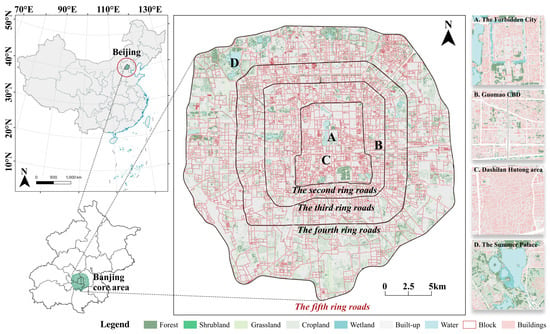
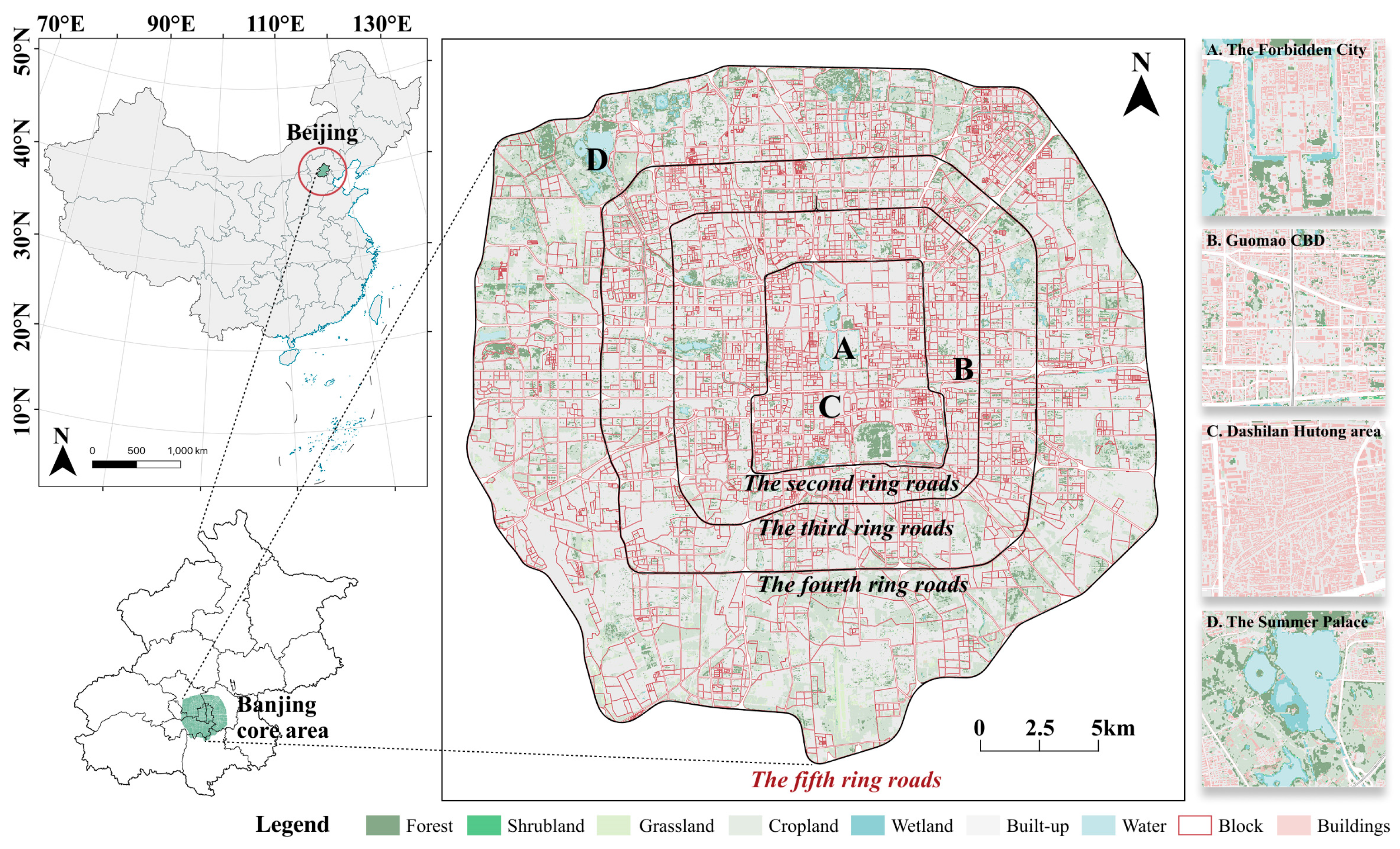
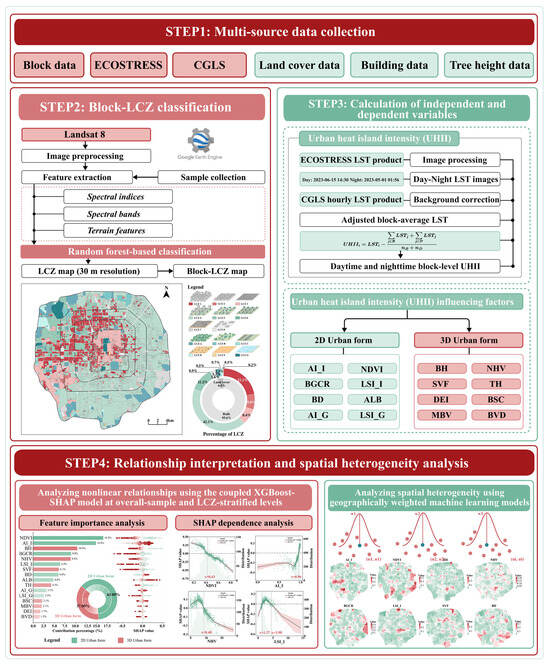
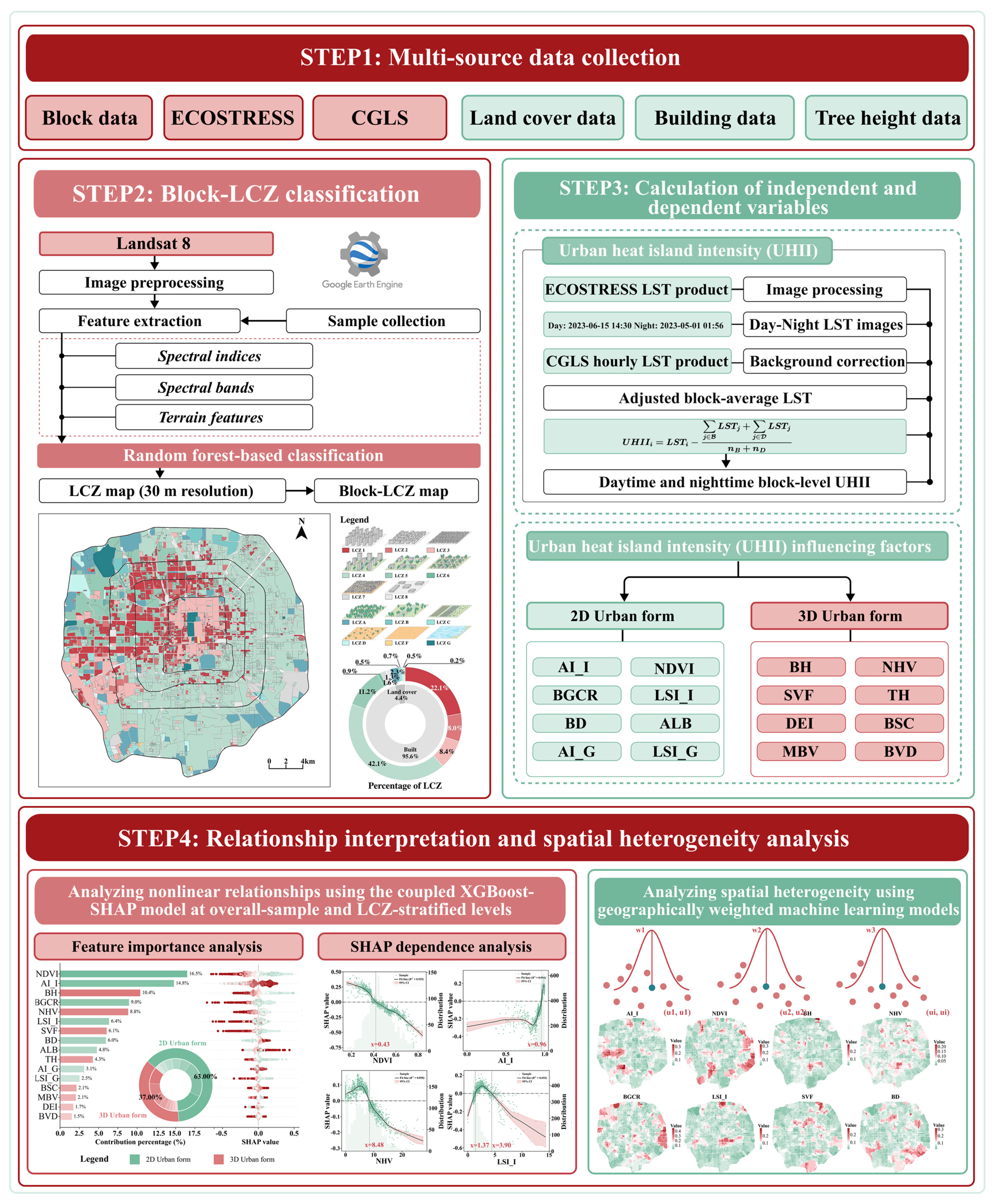
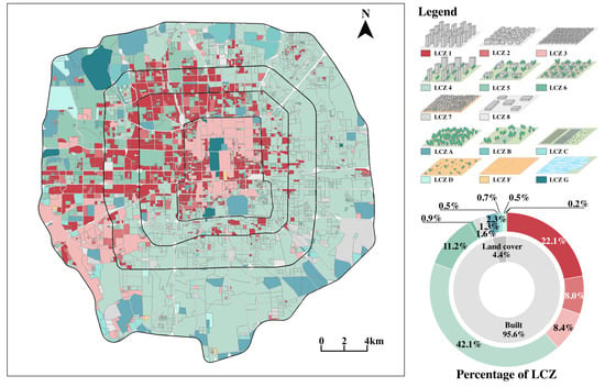
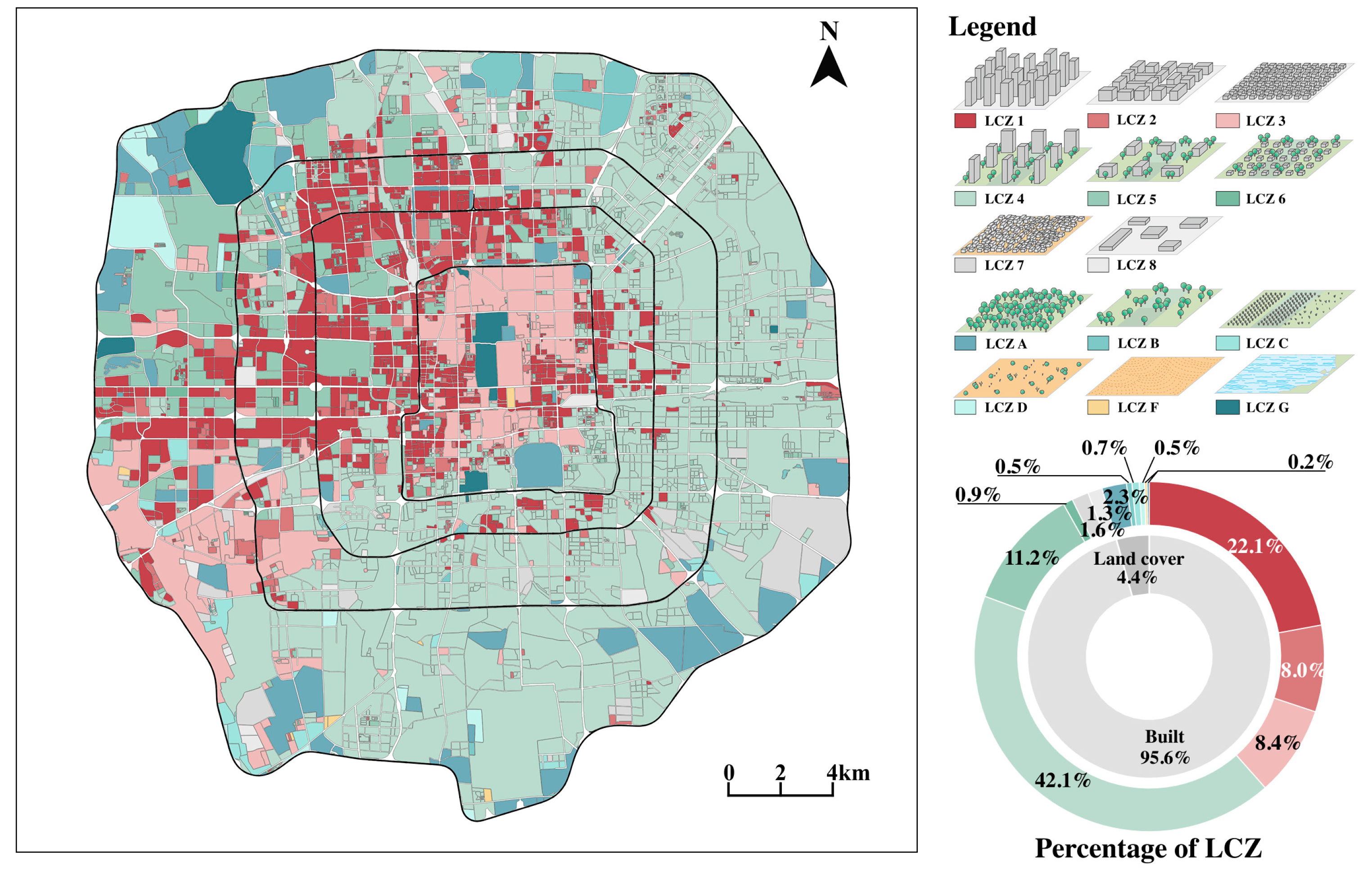
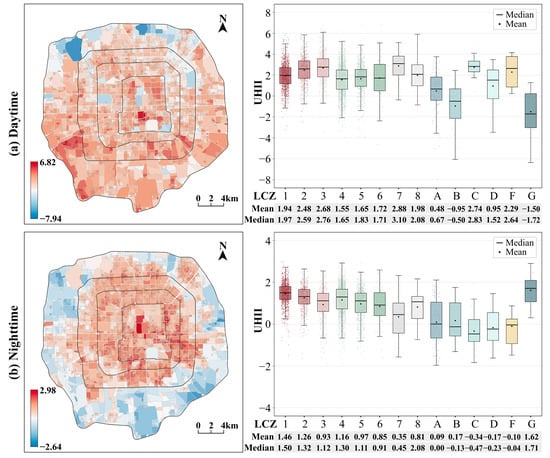
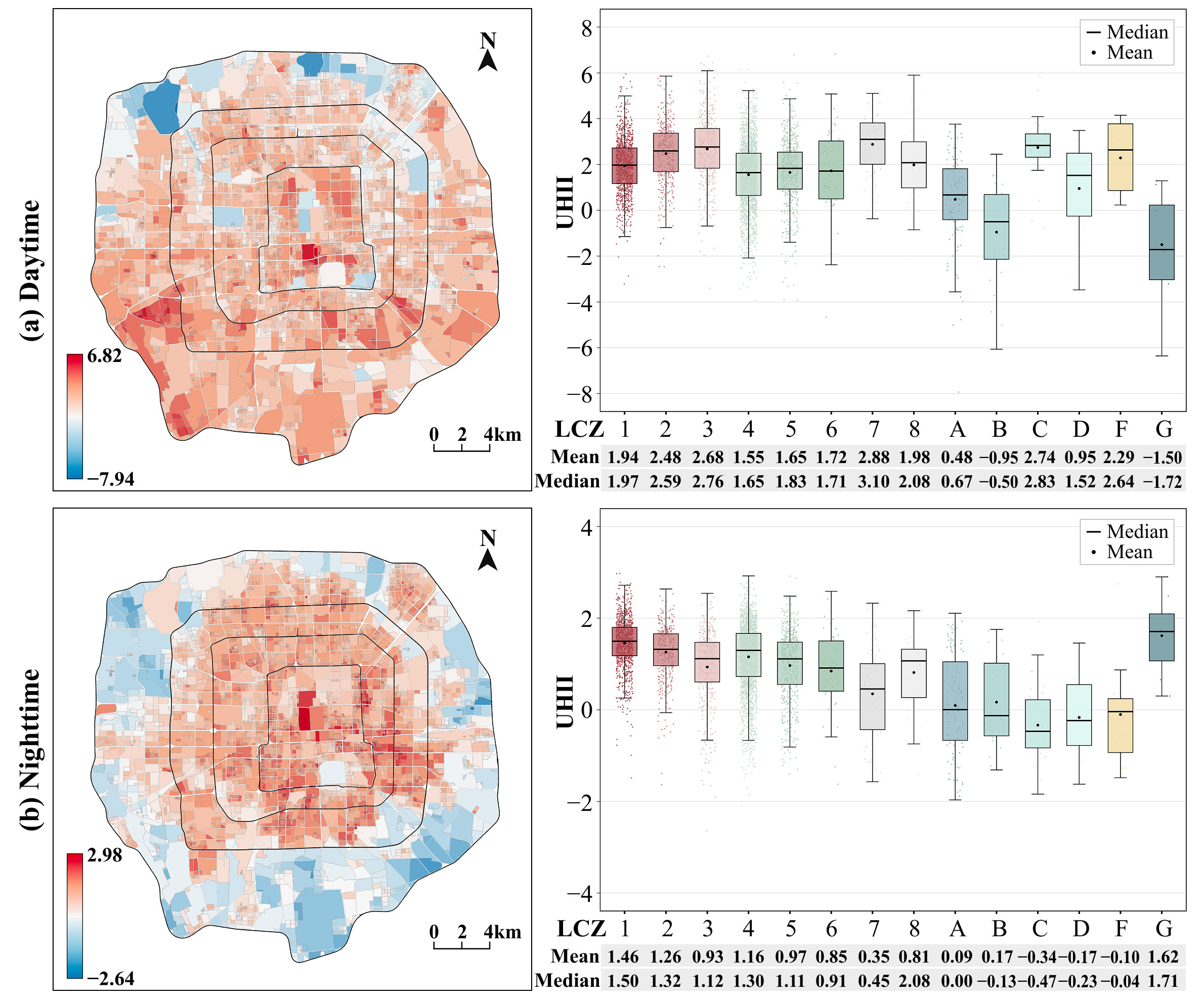
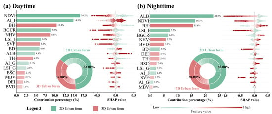
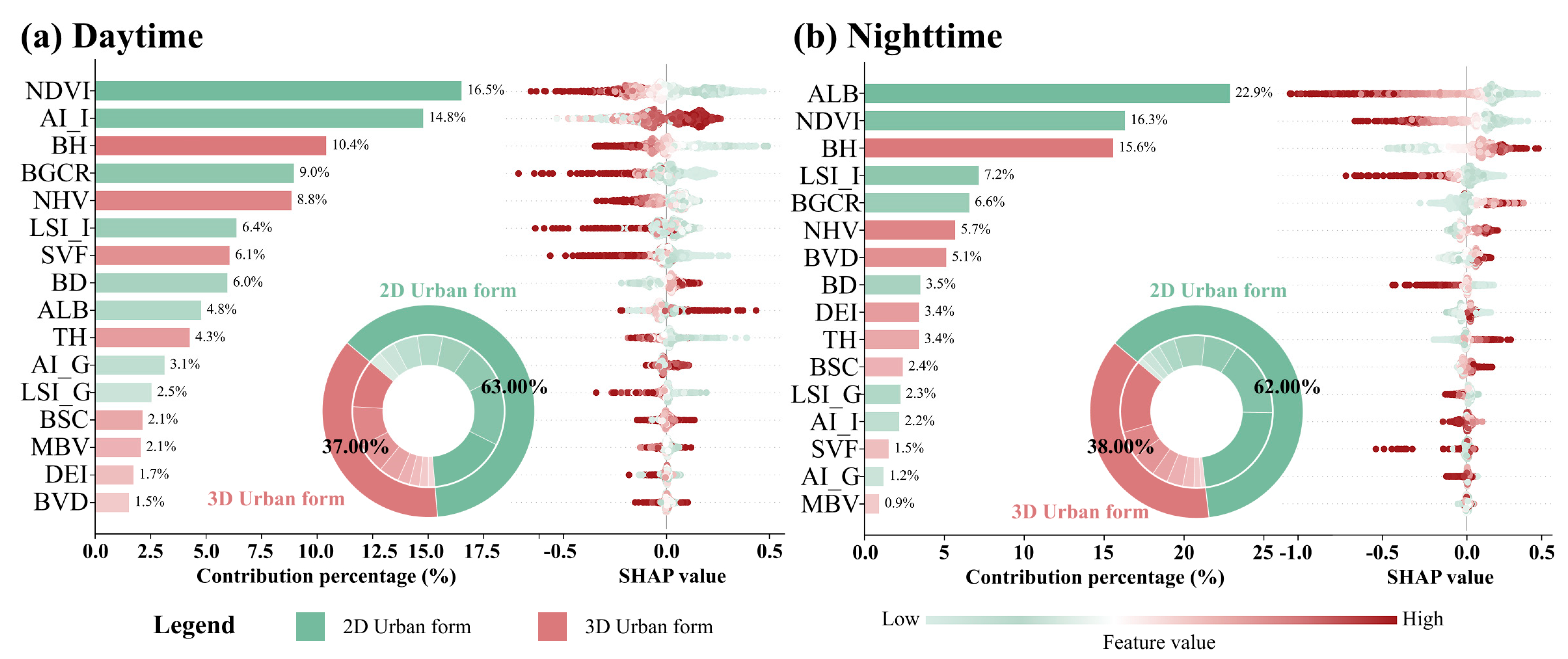
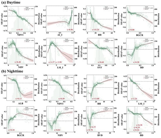
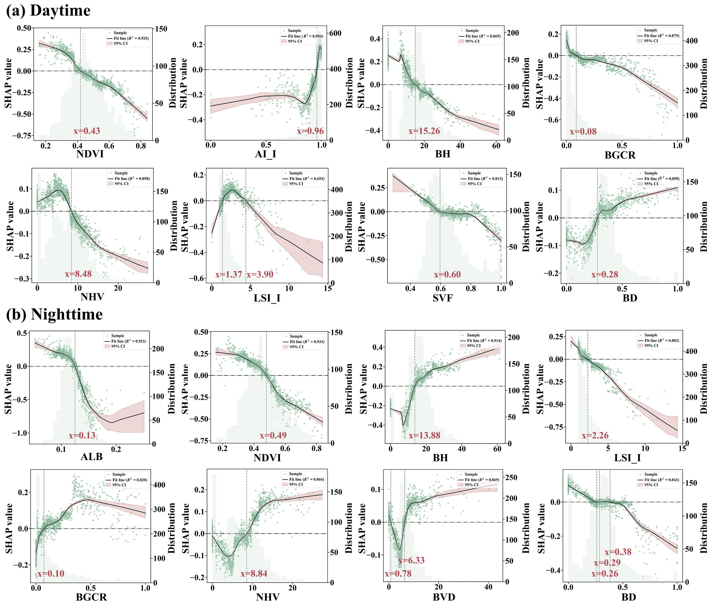
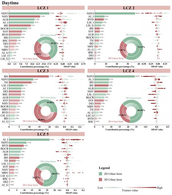
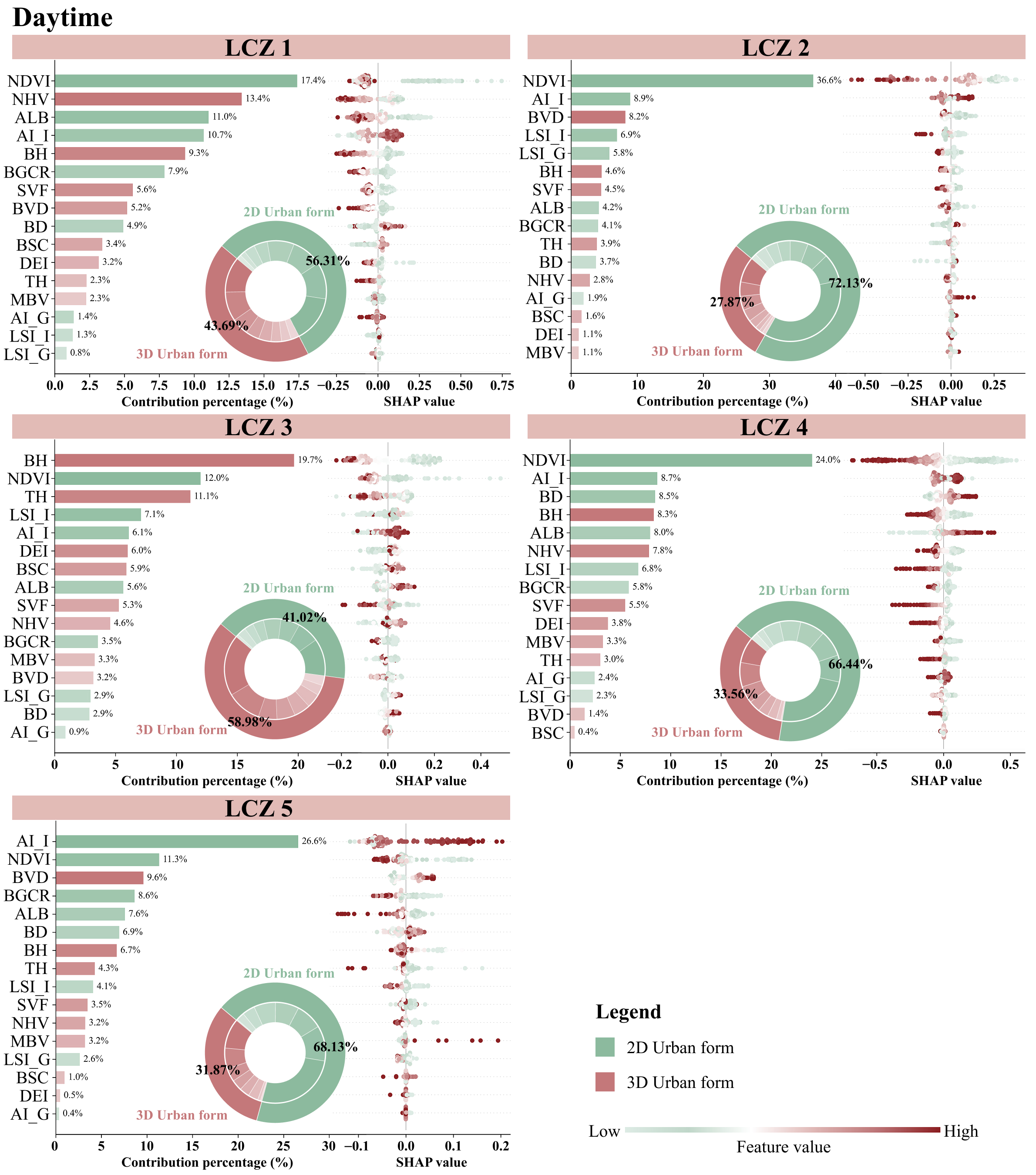
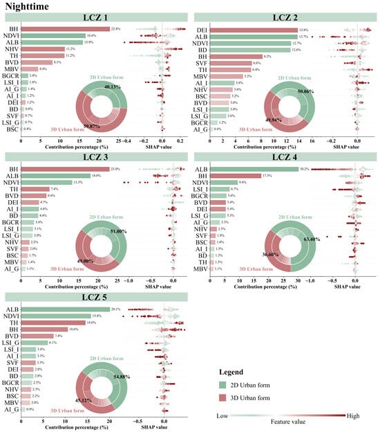
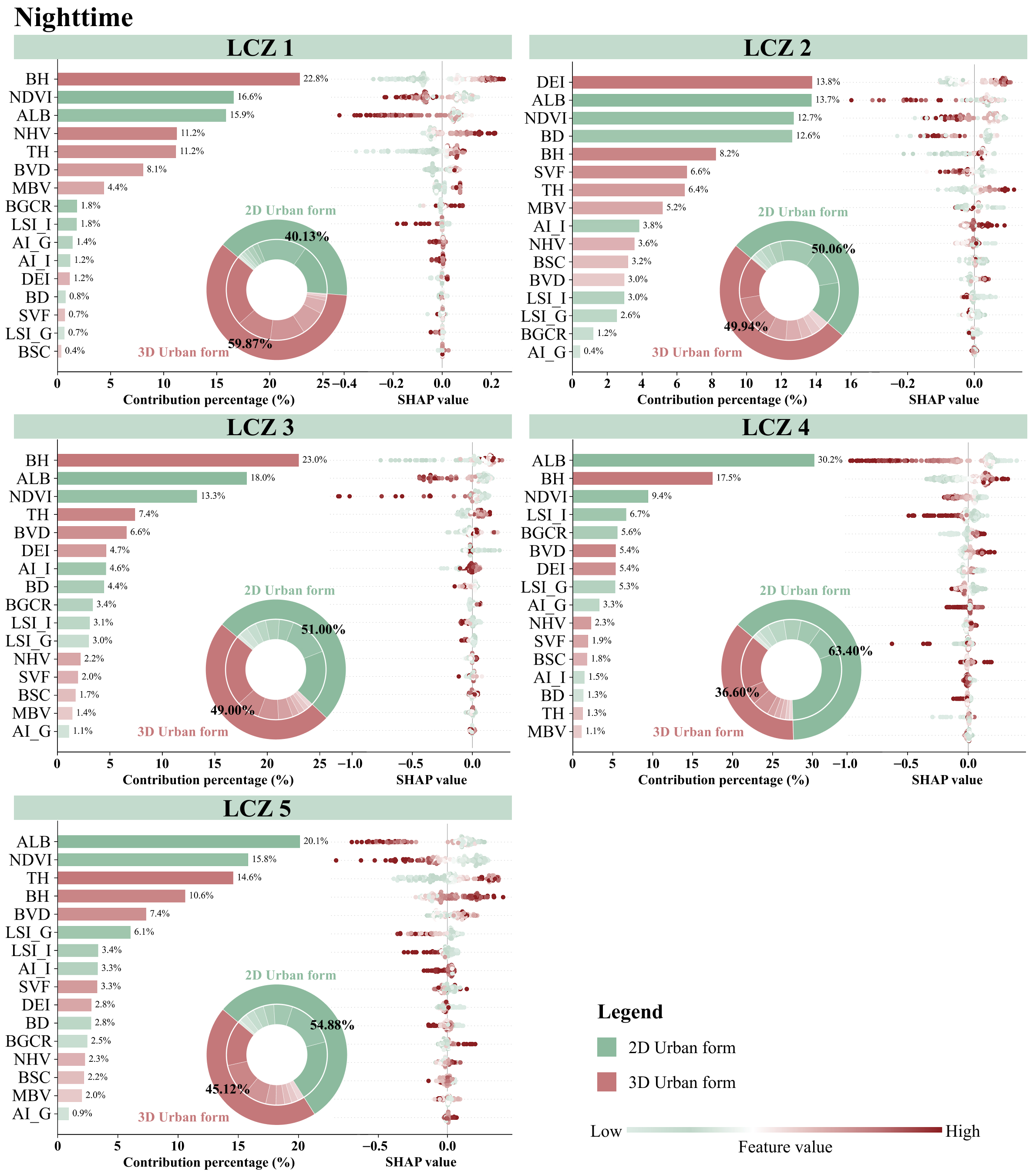
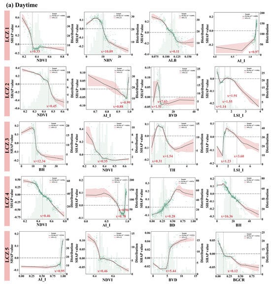
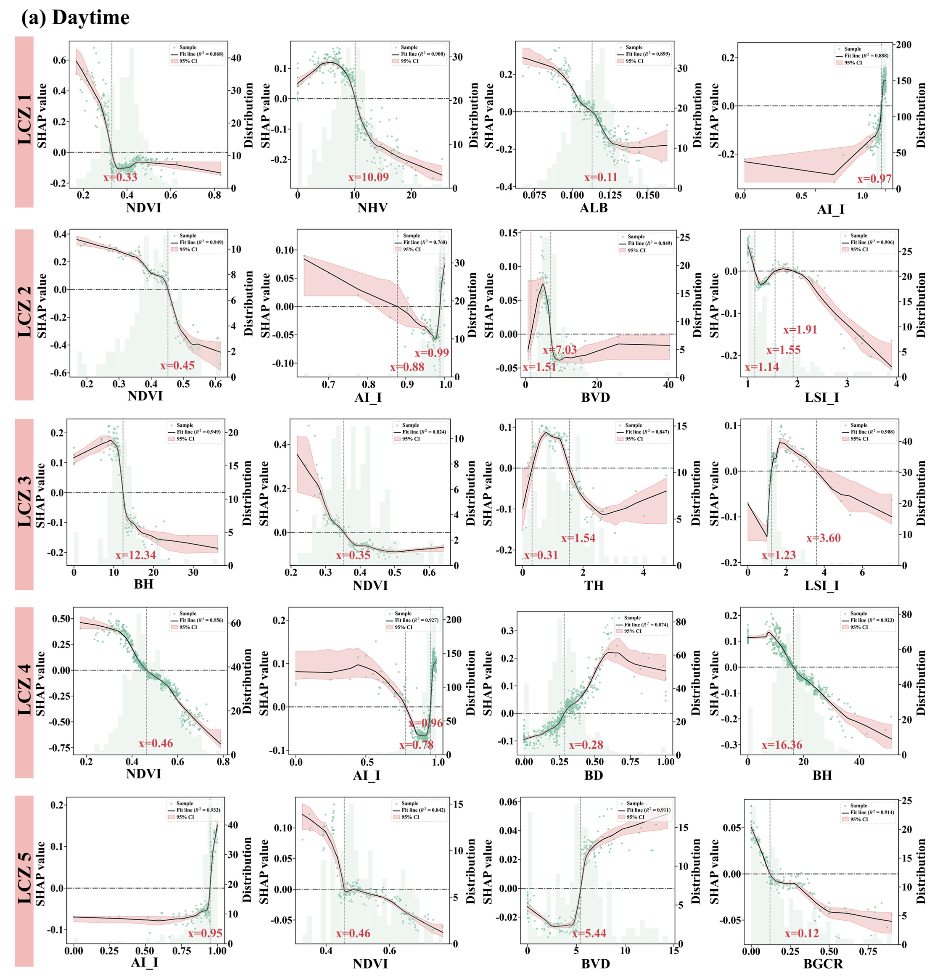
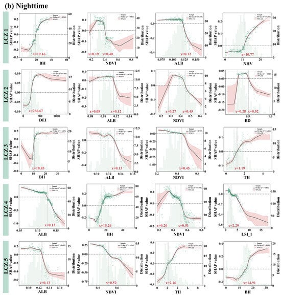
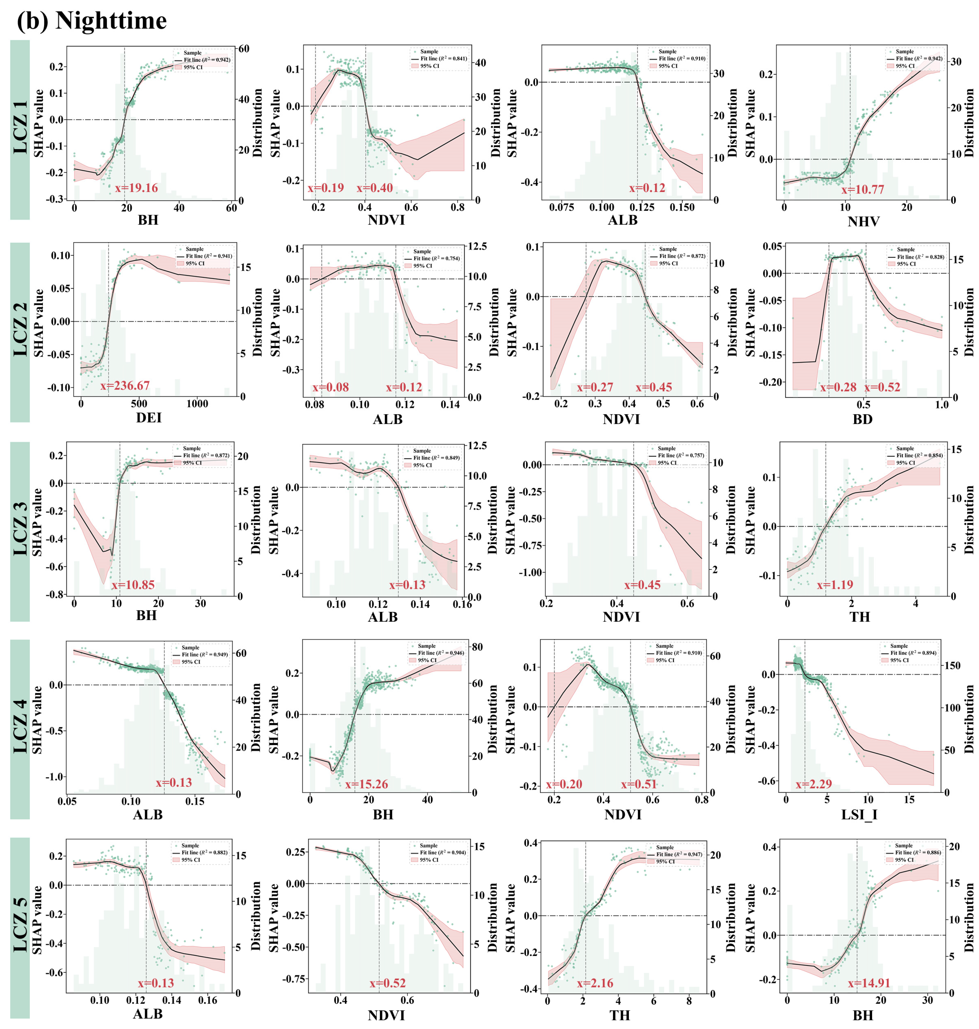
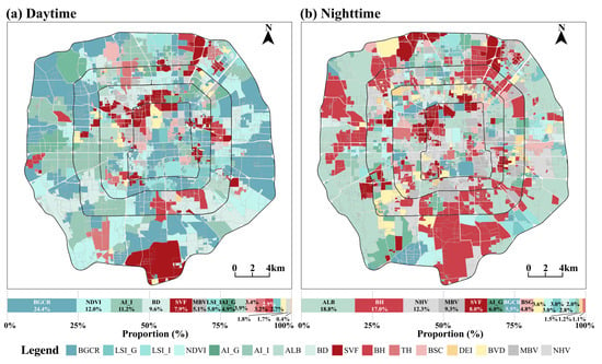
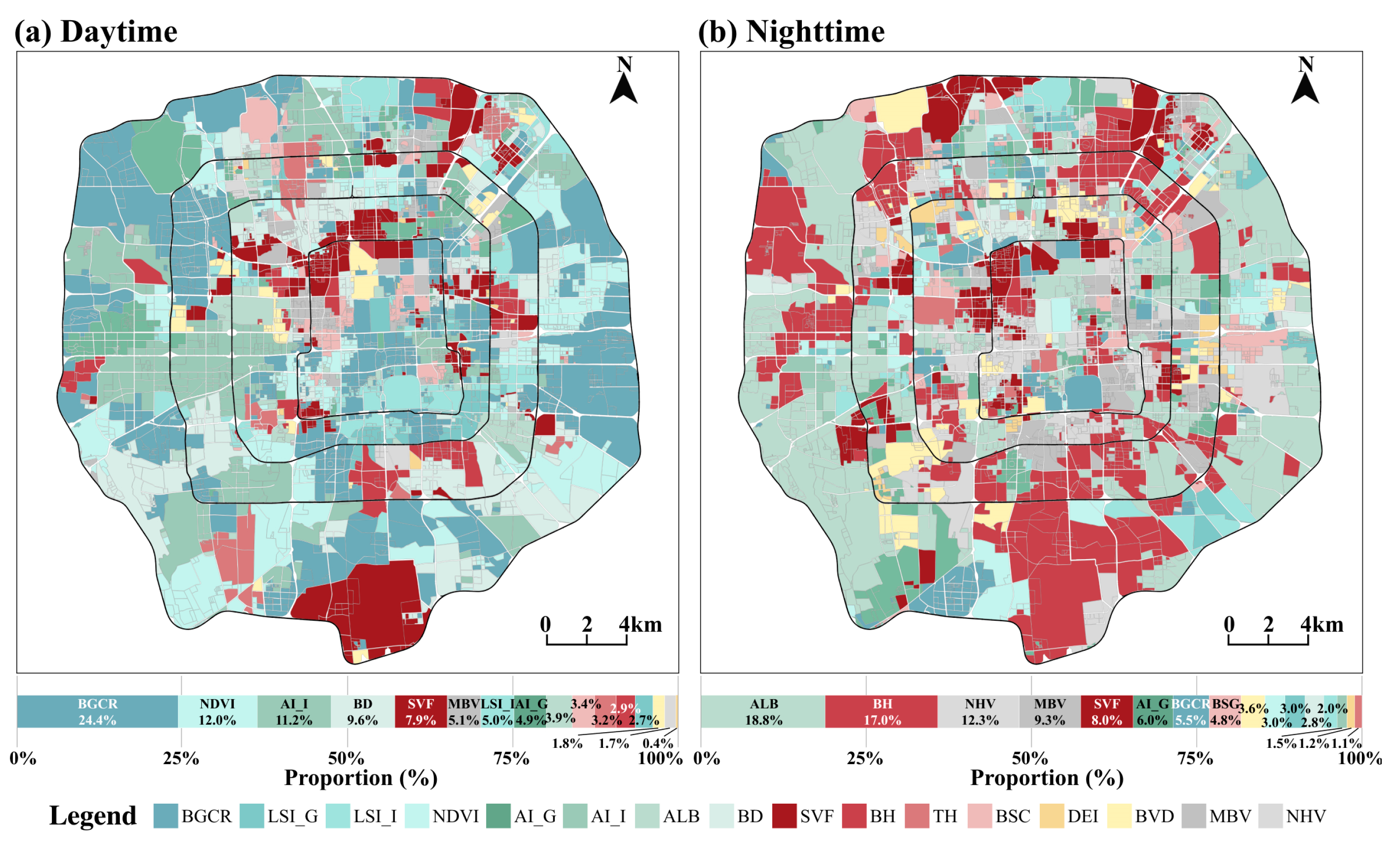
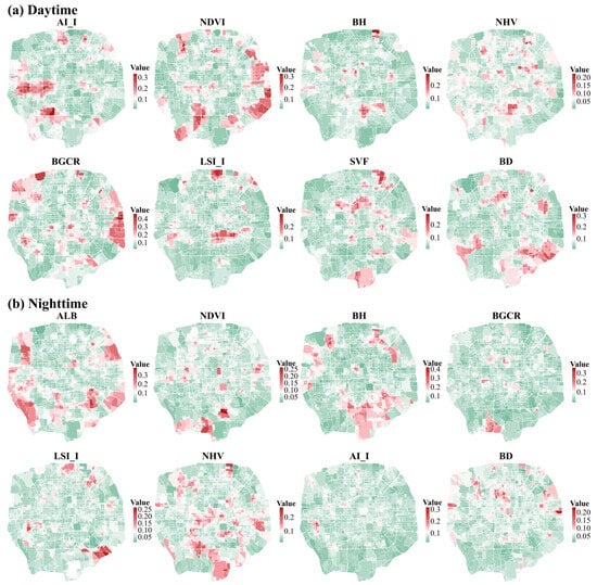
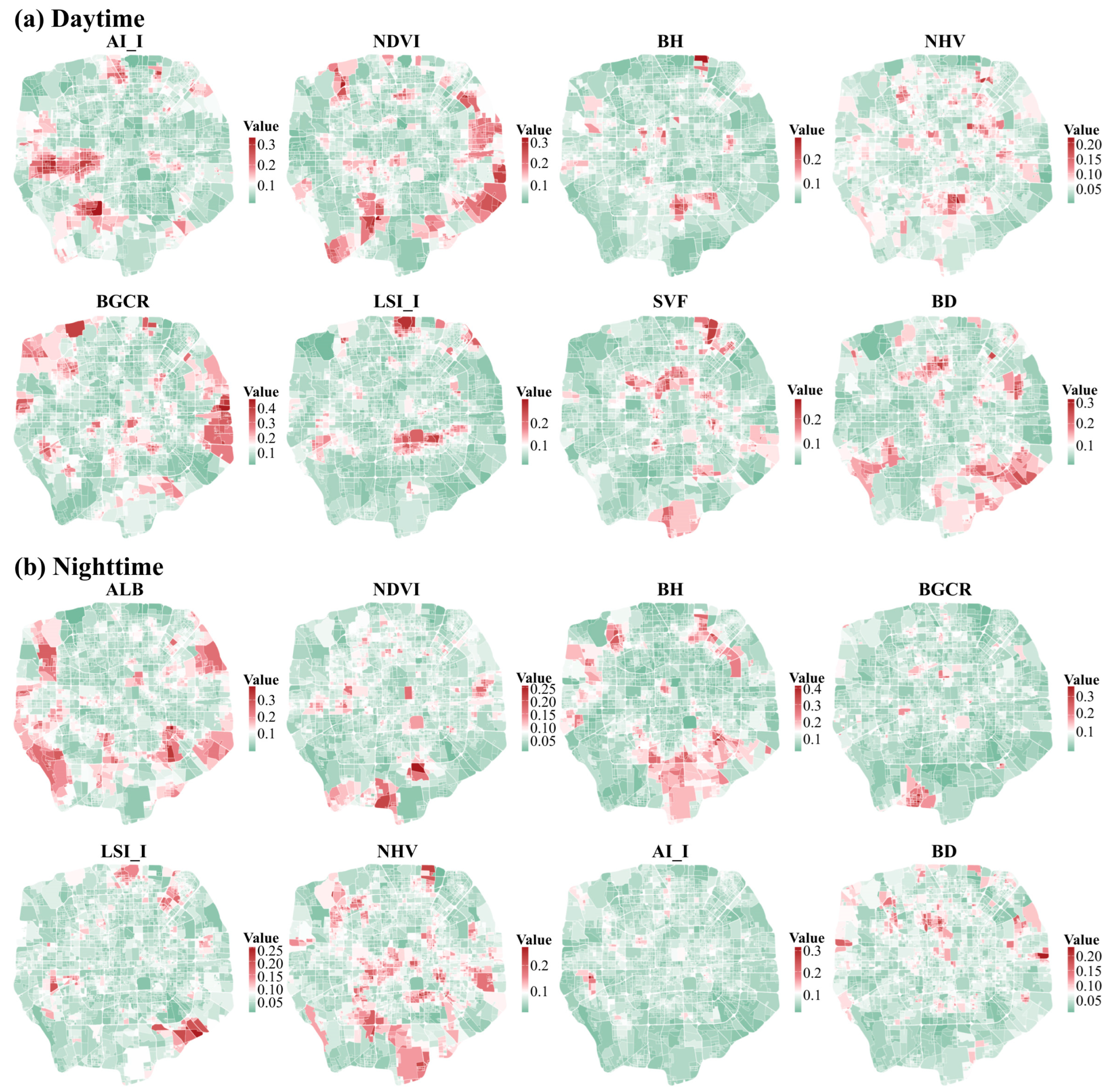

Disclaimer/Publisher’s Note: The statements, opinions and data contained in all publications are solely those of the individual author(s) and contributor(s) and not of MDPI and/or the editor(s). MDPI and/or the editor(s) disclaim responsibility for any injury to people or property resulting from any ideas, methods, instructions or products referred to in the content. |
© 2026 by the authors. Licensee MDPI, Basel, Switzerland. This article is an open access article distributed under the terms and conditions of the Creative Commons Attribution (CC BY) license.