


Abstract
Prefabricated construction relies on tightly coupled component production, transportation, and on-site installation. Local disruptions may affect project schedules via exposure, infection, recovery, and renewed susceptibility, yet the underlying dynamic mechanisms remain poorly understood. To address this gap, this study shifts the analytical focus from aggregate project schedule performance to the risk states of individual activities and the transitions between these states. A SEIRS (Susceptible–Exposed–Infected–Recovered–Susceptible)-based schedule-risk propagation model is formulated; its equilibrium points and propagation threshold are derived, and numerical scenarios are adopted to investigate the effects of risk propagation, exposure-to-infection transition, recovery, and loss of protection. Under the specified scenarios, the system converges to a nonzero-risk equilibrium when h < 1, whereas risks gradually dissipate when h ≥ 1. Variations in the propagation rate α and recovery rate γ can shift the system across the critical threshold and alter whether risks persist or dissipate. The exposure-to-infection rate β affects the manifestation of risks but does not change the ultimate risk-free outcome within the investigated parameter range. The protection-loss rate μ primarily modulates the proportions of susceptible and recovered nodes, with relatively limited effects on exposed and infected nodes. These findings indicate that schedule-risk management should integrate early propagation control, timely intervention for latent disruptions, and recovery and protection after risk infection. This study establishes a theoretical framework for understanding schedule-risk state transitions in prefabricated construction and facilitates its extended practical application.
1. Introduction
Prefabricated construction integrates industrialized production with intelligent management to improve construction efficiency while maintaining quality [1]. However, prefabricated technologies are still underdeveloped in many countries, and schedule risks often trigger delays more severe than those observed in conventional cast-in-place construction [2]. Prefabricated projects encompass design, production, transportation, storage, and on-site installation. Their schedule performance depends not only on the efficiency of individual activities but also on coordination of component supply, transportation logistics, and on-site installation demand. For example, delayed component production can progressively consume the time buffers available to subsequent transportation and installation activities, leading to component shortages or crane idle time. Such uncertainties and interdependencies enable local disruptions to propagate along activity chains, generating coupled and cascading schedule risks [3].
In recent years, prefabricated buildings have attracted substantial attention from academia and industry. Research has addressed barriers to their adoption [4], supply chain management [5], cost management [6], quality management [7], and safety management [8], thereby enriching the theoretical foundations of prefabricated construction. Nevertheless, systematic research on schedule-risk management remains underdeveloped, particularly regarding the coupling of schedule risks in prefabricated projects [3]. Existing risk analyses are also predominantly static and pay insufficient attention to dynamic behavior and feedback mechanisms over time. Accordingly, this study adopts the SEIRS (Susceptible–Exposed–Infected–Recovered–Susceptible) model to investigate the formation and complex dynamic evolution of schedule risks in prefabricated construction, yielding theoretical and practical implications for its sustainable development.
The remainder of this paper is organized as follows. Section 2 reviews research on schedule risks in prefabricated construction and risk-propagation models in construction engineering. Section 3 analyzes the schedule-risk propagation process. Section 4 presents the research methodology, and Section 5 reports the numerical simulations and results. Section 6 discusses the risk-evolution mechanisms and managerial implications of the threshold scenarios and parameter variations. Section 7 summarizes the conclusions and limitations.
2. Literature Review
2.1. Schedule Risks in Prefabricated Construction
Construction schedule-delay analysis examines deviations between planned and actual progress, alongside their causes and allocation of responsibility [9]. Despite extensive research, delays remain prevalent across the global construction sector, leading to schedule slippage, cost overruns, and resource wastage [9]. Prefabricated construction requires coordination among factory production, logistics, and on-site work and it diverges from conventional construction in manufacturing procedures, workflows and technical arrangements, which raises its vulnerability to delays [10]. Accurately identifying schedule-risk factors is therefore a prerequisite for delay mitigation. Abdul Nabi et al. (2021) combined a literature review and questionnaire survey to identify eight critical factors affecting the schedules of prefabricated projects [11]. Cho et al. (2021) used qualitative comparative analysis (QCA) of prefabricated-construction cases to determine the relationships between project conditions and actual schedule delays [12].
The coupled effects of multiple risk factors can exacerbate schedule delays more than their simple additive effects. Their interrelationships during construction therefore need to be examined. Li et al. (2016) applied social network analysis (SNA) to evaluate schedule-risk factors and their relational networks in prefabricated projects [13]. Fan et al. (2022) analyzed the causal relationships and the strength of influence among key delay factors to identify the most critical factors [3]. Li et al. (2018) used a hybrid dynamic model to investigate how dynamic interactions among risk factors affect project schedule performance [14]. Abdul Nabi et al. (2022) applied a weighted-average method to calculate relative risk weights and quantify the influence of individual factors on schedule performance in prefabricated construction [15].
2.2. Risk-Propagation Models in Construction Management
The schedule-risk system for prefabricated construction is complex, comprising numerous risk factors and their interactions. Complex-network theory provides an effective means of revealing the internal structures and relationships of such systems. Risk-evolution studies based on complex networks have therefore laid important methodological foundations for this research. Interpretive structural modeling [3], DEMATEL [1], Bayesian networks [16], system dynamics [14], and social network analysis [13], for example, have been used to analyze risk relationships, pathways, and degrees of influence. However, dynamic risk propagation remains insufficiently addressed in these studies.
Epidemic-dynamics models are mathematical tools for studying transmission processes. With advances in epidemic modelling theory, their applications have extended beyond disease transmission in human populations to risk propagation in engineering systems. He et al. (2021) developed an improved SIR (Susceptible–Infected–Removed) model to analyze social-stability risk diffusion in large complex engineering projects [17]. Xu et al. (2023) applied a SEIRS model to risk transmission in urban river ecological-management projects, examining propagation delays and the influence of latent nodes [18]. Zhang et al. (2023) used an SIR model to examine factors affecting the diffusion of green behavior among contractors and to simulate alternative diffusion pathways [19]. Collectively, these studies demonstrate the value of epidemic-dynamics models for understanding and managing dynamic schedule-risk propagation in prefabricated construction.
2.3. Research Gaps
Previous studies have identified factors associated with schedule delays in prefabricated construction and examined their interdependencies. Epidemic models have also been used to investigate dynamic risk propagation in engineering projects, including the role of latent risk. However, how local disruptions evolve across activity-level risk states in prefabricated construction remains insufficiently understood, particularly when coordination among component production, transportation, and installation allows some disruptions to be resolved before they delay downstream work. To address this gap, this study uses a SEIRS model to track the aggregate evolution of activity-level risk states and examines how transitions out of the latent state affect whether risk persists and the proportion of activities affected when it does.
3. Analysis of Schedule Risk Propagation in Prefabricated Building Projects
In this study, a node represents an observable schedule-related activity or process in prefabricated construction, such as the production or transportation of a batch of precast components or their on-site lifting operation. The model describes system evolution in terms of the proportions of such nodes in different risk states. Table 1 defines these states.
Table 1.
Definitions of risk-node states.
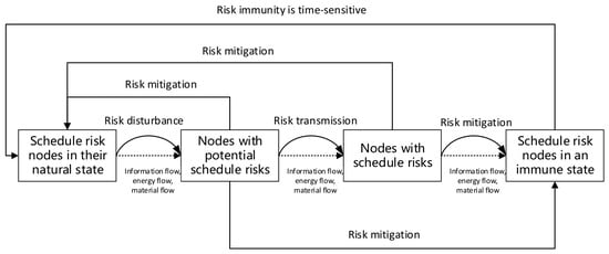
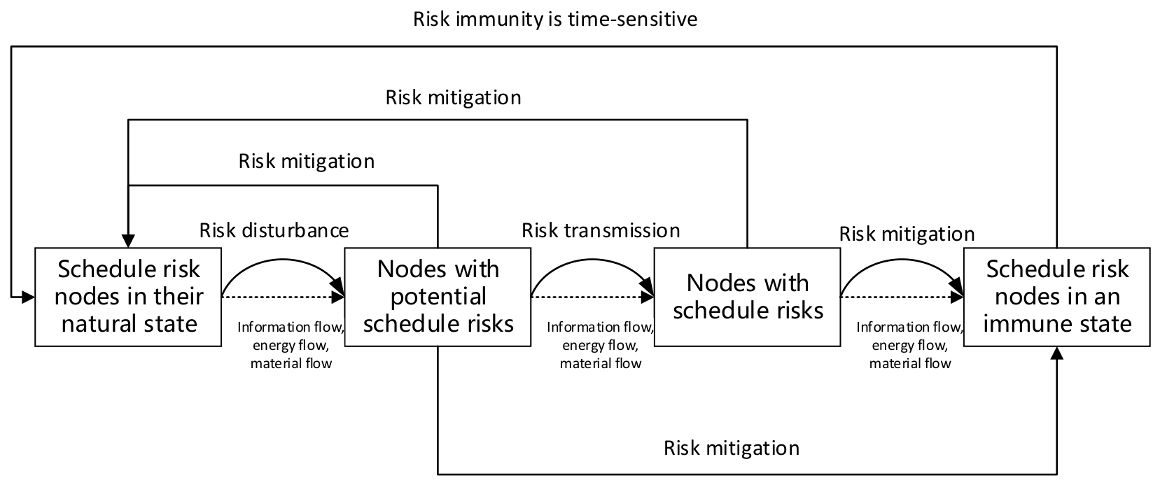
In the schedule-risk network of prefabricated construction, risk factors are connected through the orderly flows of information, materials, and energy. Nodes in the susceptible state face potential threats and disturbances and may therefore develop or be affected by risks. Exposed nodes have encountered risks that have not yet become manifest. Such nodes may possess relatively strong risk resistance or may have been treated through interventions that prevent further propagation. However, resistance varies among nodes. If risks are not effectively controlled, they can travel along inter-node paths, gradually propagate, and ultimately affect the overall schedule of prefabricated construction. Nodes that have mitigated the adverse effects of risks return to a normal, stable state and acquire experience that provides temporary protection against future risks. Over time, however, changes in the external environment or internal conditions can undermine preventive measures, causing nodes to lose protection and become susceptible again. Figure 1 illustrates this schedule-risk propagation process.
Figure 1.
Schedule-risk propagation process in prefabricated construction.
Consider the interface among component production, transportation, and installation. Delayed production may move transportation into the exposed state. If production or transportation arrangements are adjusted promptly enough to absorb the disruption, transportation can return to the susceptible state or enter a recovered, temporarily protected state after effective backup arrangements are established. If the disruption exceeds the available buffer and produces a defined schedule abnormality, the process enters the infected state. Once the abnormality is resolved, the process may recover without sustained protection or recover with additional protective measures. Withdrawal of backup resources, changes in operating conditions, or failure of these measures can return the recovered process to the susceptible state.
4. Research Methodology
4.1. Model Assumptions
The SEIRS model provides a framework for describing transitions among susceptible, exposed, infected, and recovered states. This study extends its application to schedule-risk evolution in prefabricated construction, thereby providing a quantitative approach to risk propagation. Based on epidemic-transmission principles [19,20], the model is developed under the following assumptions.
Assumption 1.
At time t, S(t), E(t), I(t), and R(t) denote the proportions of susceptible, exposed, infected, and recovered nodes, respectively, in the network. These proportions satisfy S(t) + E(t) + I(t) + R(t) = 1, and all four functions are continuous and differentiable with respect to t.
Assumption 2.
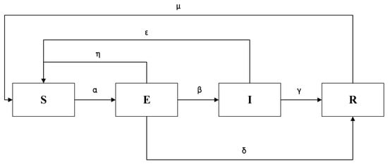
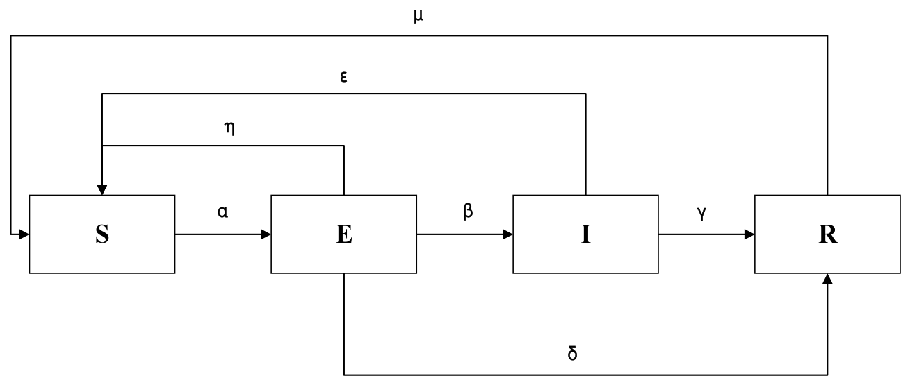
The transition rates are defined as follows: α, from susceptible to exposed; β, denotes the rate from exposed to infected; γ, from infected to recovered; μ, from recovered to susceptible; ε, spontaneous recovery from infected to susceptible; η, from exposed to susceptible; and δ, direct transition from exposed to recovered. All parameters take nonnegative real numbers, where α > 0, β > 0, μ > 0, and γ + ε > 0.
Assumption 3.
Construction activities are the units to which risk states are assigned, while the model describes the evolution of the overall proportions of activities in these states. In the absence of project-specific data on activity dependencies, we use a homogeneous-mixing approximation to examine system-level risk trajectories and persistence conditions. Under this approximation, susceptible activities face the same modeled exposure rate at a given time. This is a simplification for aggregate analysis and does not imply that actual dependencies among fabrication, transportation, and installation activities are uniform.
Under these assumptions, a schedule-risk propagation model based on SEIRS is established to analyze risk-transmission patterns and evolutionary processes in the schedule-risk network of prefabricated construction. Figure 2 illustrates the state-transition process.
Figure 2.
State-transition process of the SEIRS model.
4.2. Model Construction
Based on epidemic-dynamics modeling principles and related studies, the following system of differential equations is formulated to describe schedule-risk propagation in construction projects:
The term αSI represents the aggregate flow of activities from the susceptible state to the exposed state. Here, α is an effective propagation rate, and the per-activity exposure rate αI depends on the overall infected proportion rather than on the states of explicitly linked upstream activities.
Under Assumption 1, the state proportions satisfy the following normalization condition:
This study investigates the mechanisms by which risks disrupt schedule performance in prefabricated projects, focusing on propagation rate, duration, and scope. Determining the equilibrium points and critical threshold is essential for understanding these phenomena. These equilibrium points and the critical threshold reveal schedule-risk propagation patterns and trends, providing a theoretical basis for construction management and risk control.
4.3. Analysis of Equilibrium Points and Thresholds in Schedule Risk Propagation
In the schedule-risk network of prefabricated construction, nodes affected by schedule disruptions can influence downstream nodes over time. Whether risks continue to propagate or dissipate depends on the propagation threshold h. Let a = β + η + δ and b = γ + ε. For all four components of the positive equilibrium to be positive, δb/β + γ > 0 must also hold. Time t may be expressed in arbitrary units. In a fully susceptible population, an infected node remains infected for an average duration of 1/b and generates α new exposed nodes per unit time. A fraction β/a of these nodes subsequently enters the infected state. The basic risk-reproduction number is therefore defined as R0 = αβ/(ab), with h = 1/R0 = ab/(αβ). Here, R0 describes invasion in a fully susceptible population, whereas the instantaneous effective quantity is Re(t) = R0S(t). The effective reproduction quantity alone does not fully summarize the transient process; in particular, Re < 1 does not imply that existing exposed units disappear immediately.
Because the prefabricated-construction schedule-risk network is bounded, all initial values must lie within the following region:
(1) Risk-free equilibrium. When the numbers of exposed, infected, and recovered nodes are all zero, every node in the network is susceptible and unaffected by schedule risk, and no risk propagation occurs. The system therefore has the risk-free equilibrium P0 = (1, 0, 0, 0).
(2) Nonzero equilibrium. The risk-free equilibrium (1, 0, 0, 0) is an idealized state that is generally unattainable in practice. It is therefore necessary to identify nonzero equilibria within the bounded region D. Setting the time derivatives to zero yields:
Substituting the normalization condition in Equation (2) into these expressions gives:
where
Here, h denotes the schedule-risk propagation threshold.
Accordingly, a unique positive equilibrium (S*, E*, I*, R*) exists within D when h < 1, whereas no positive equilibrium exists when h ≥ 1.
The characteristic polynomial of the constrained Jacobian matrix at P0 is . When h > 1, all eigenvalues have negative real parts; when h < 1, a positive eigenvalue exists. At h = 1, the linearization has a zero eigenvalue, so stability requires a separate argument. Taking gives , so V′ ≤ 0 for h ≥ 1. When h > 1, V′ = 0 requires I = 0, and maintaining I = 0 further requires E = 0; the remaining equation then drives the state toward P0. When h = 1, S = 1 implies E = I = R = 0, and the I = 0 branch likewise converges ultimately to P0. Since V constrains E and I, while the stable linear equation for R keeps R small under small perturbations, the compact, positively invariant region D and the invariance principle together establish that P0 is globally asymptotically stable for h ≥ 1. Moreover, P0 remains a feasible equilibrium throughout.
Therefore, when h ≥ 1, the risk-free equilibrium is the only equilibrium, and schedule risks gradually dissipate over time. When h < 1, the system has a unique positive equilibrium (S*, E*, I*, R*). In the absence of control measures, schedule risks can therefore persist at non-zero levels and ultimately impair the overall progress of prefabricated construction.
5. Simulation and Results Analysis
5.1. Impact of Thresholds on Risk Propagation Behavior
Based on the theoretical analysis, MATLAB R2023a simulations are used to examine how the threshold and individual parameters affect risk propagation in prefabricated construction. For all simulations presented below, the governing differential equations were integrated in MATLAB R2023a using the adaptive Runge–Kutta solver ode45 with default solver settings. Each simulation used the interval t ∈ [0,100] in model time units and the initial state ((S(0),E(0),I(0),R(0)) = (0.99,0.01,0,0)). Because empirical data on micro-level risk propagation are difficult to obtain, hypothetical parameter values are specified to represent plausible scenarios. Such scenario-based simulations allow alternative risk conditions and theoretical propositions to be examined systematically, which is essential for understanding complex-system behavior.
(1) Propagation threshold h < 1. To examine the dynamic evolution of risk states after a small number of latent disruptions enter the system, a baseline scenario is constructed with low initial exposure, sufficient propagation potential, and temporarily effective protection. The initial state is S0 = 0.99, E0 = 0.01, I0 = 0, and R0 = 0. Thus, most process units are initially unaffected, while a small proportion are exposed but have not yet developed infection risks or entered a recovered state. This setting represents a small initial disturbance that may subsequently affect other processes.
Parameter values are selected to represent the transition mechanisms and relative rates in this scenario. Setting α = 0.5 and β = 0.5 represents latent disruptions with some capacity to propagate and become manifest. Setting γ = 0.2 and ε = 0.05 makes recovery with temporary protection more likely than direct return to susceptibility after manifestation. Setting δ = 0.1 and η = 0.05 represents early treatment of latent disruptions, including the possibility of temporary protection. Finally, μ = 0.1 allows protection to fail as operating conditions change, returning processes to the susceptible state. Equation (6) yields h = 0.65 < 1. Figure 3 shows the resulting schedule-risk propagation behavior.
Figure 3.
Effects of h < 1 on schedule-risk propagation.
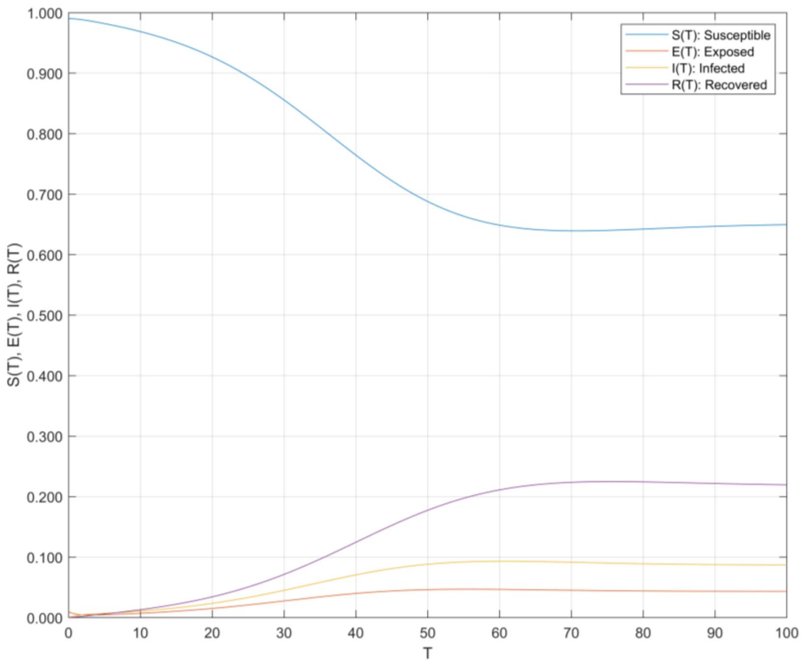
As shown in Figure 3, when h = 0.65 < 1, the proportion of susceptible nodes gradually decreases, whereas the proportions of exposed, infected, and recovered nodes increase from their initial levels and stabilize after moderate fluctuations. Notably, the exposed and infected proportions do not converge to zero, indicating a persistent non-zero risk state.
(2) Propagation threshold h ≥ 1. For comparison with the persistent-risk scenario, a second scenario is constructed with weaker propagation, stronger risk mitigation, and longer-lasting protection. The initial proportions remain S0 = 0.99, E0 = 0.01, I0 = 0, and R0 = 0 so that both scenarios begin with the same disturbance.
The parameters α and β are reduced from 0.5 to 0.45, representing lower transition rates from susceptible to exposed and from exposed to infected, respectively. The parameter γ is increased from 0.2 to 0.25, and ε is increased from 0.05 to 0.15. These changes increase the overall rate at which infected nodes transition to either the recovered or susceptible state, shortening the average duration of infection. The parameter η is increased from 0.05 to 0.1, while δ remains 0.1, increasing the overall rate at which latent disruptions are resolved before manifestation. Finally, μ is reduced from 0.1 to 0.05 so that temporary protection lasts longer. These relative rates represent suppressed propagation, timely risk treatment, and durable protection. Equation (6) yields h = 1.28 ≥ 1. Figure 4 shows the resulting schedule-risk propagation behavior.
Figure 4.
Effects of h ≥ 1 on schedule-risk propagation.
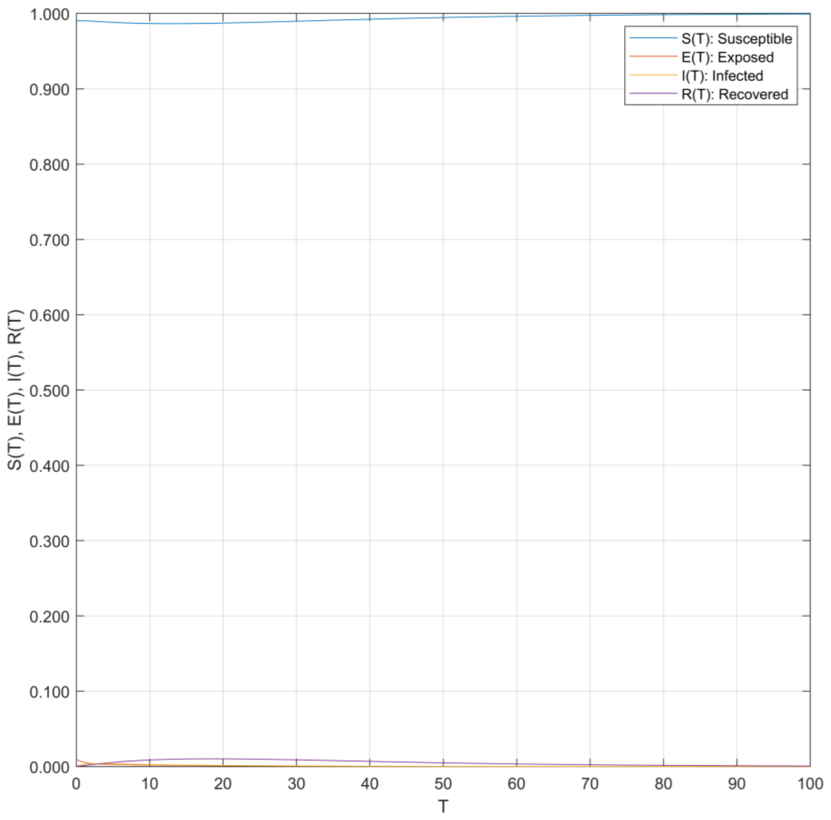
As shown in Figure 4, when h = 1.28 ≥ 1, the susceptible proportion returns gradually to 1 after a short-term change, while the exposed, infected, and recovered proportions all approach zero. In contrast to the scenario depicted in Figure 3, this scenario does not sustain nonzero exposed or infected proportions; instead, the system ultimately approaches the risk-free equilibrium.
5.2. Impact of Various Parameters on Risk Propagation Behavior
Under normal conditions, institutional and regulatory constraints generally keep prefabricated projects in a relatively healthy state. Subsequent analyses therefore use the h ≥ 1 scenario in Figure 4 as the baseline. Preliminary simulations of η, ε, and δ produced similar system responses; these parameters were therefore excluded from the subsequent one-at-a-time analysis. The key parameters α, β, γ, and μ are varied to observe changes in the four state proportions and identify the principal factors affecting schedule-risk propagation.
(1) Effect of α. The parameter α is the transition rate from the susceptible to the exposed state. The values α = 0.1, 0.45, 0.7, and 0.9 are tested separately to examine network dynamics under different propagation intensities. Figure 5 shows the resulting effects on schedule-risk propagation in prefabricated construction.
Figure 5.
Effects of α on schedule-risk propagation.
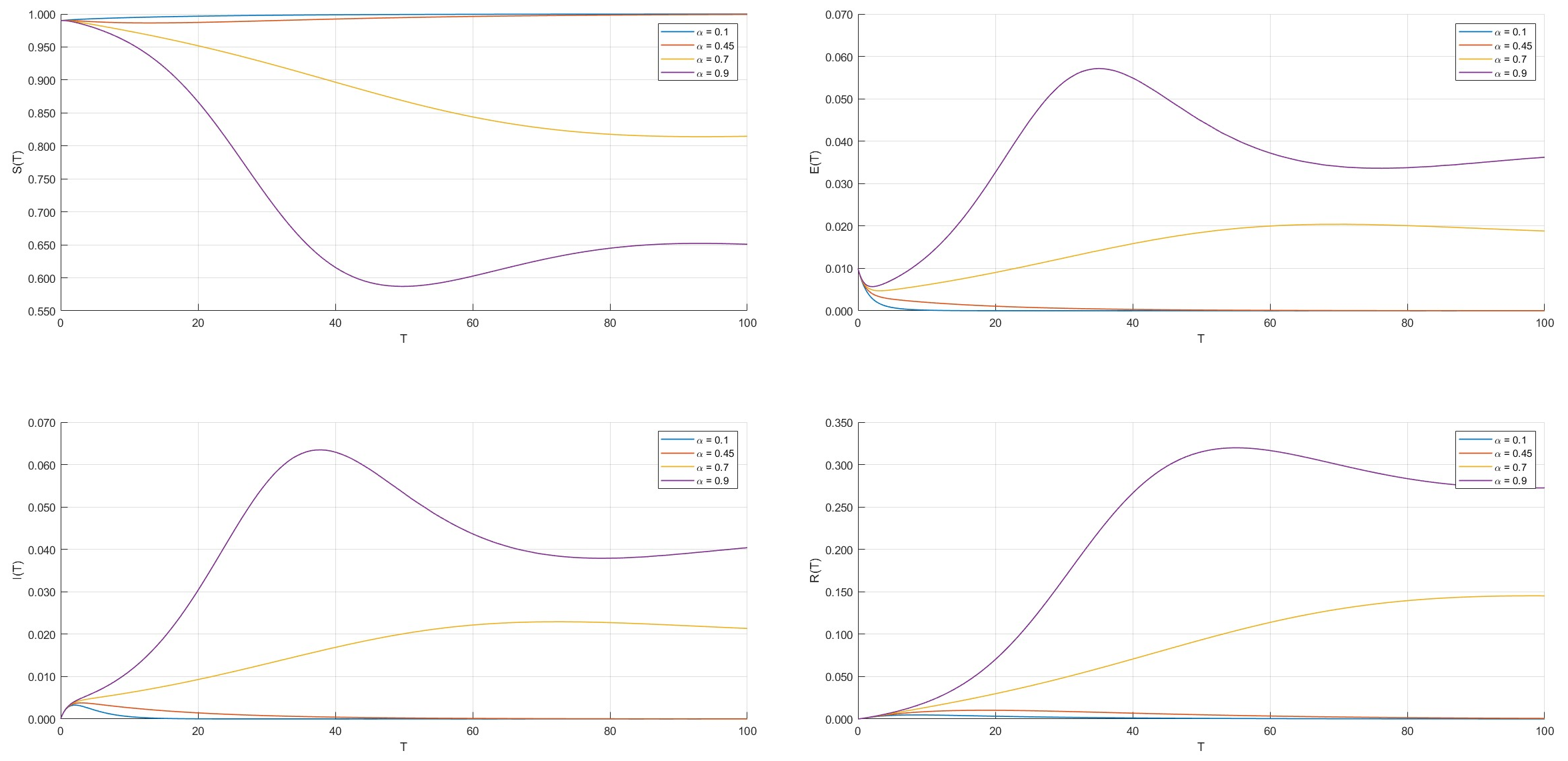
As shown in Figure 5, when α = 0.1 or 0.45, the four state proportions change relatively modestly; S(t) subsequently approaches 1, while E(t), I(t), and R(t) approach 0. When α increases to 0.7 or 0.9, the decline in S(t) and the variations in E(t), I(t), and R(t) become more pronounced, and the exposed and infected proportions remain nonzero near the end of the simulation.
(2) Effect of β. The parameter β is the transition rate from the exposed to the infected state. The values β = 0.1, 0.45, 0.7, and 0.9 are tested separately, and their effects on schedule-risk propagation are shown in Figure 6.
Figure 6.
Effects of β on schedule-risk propagation.
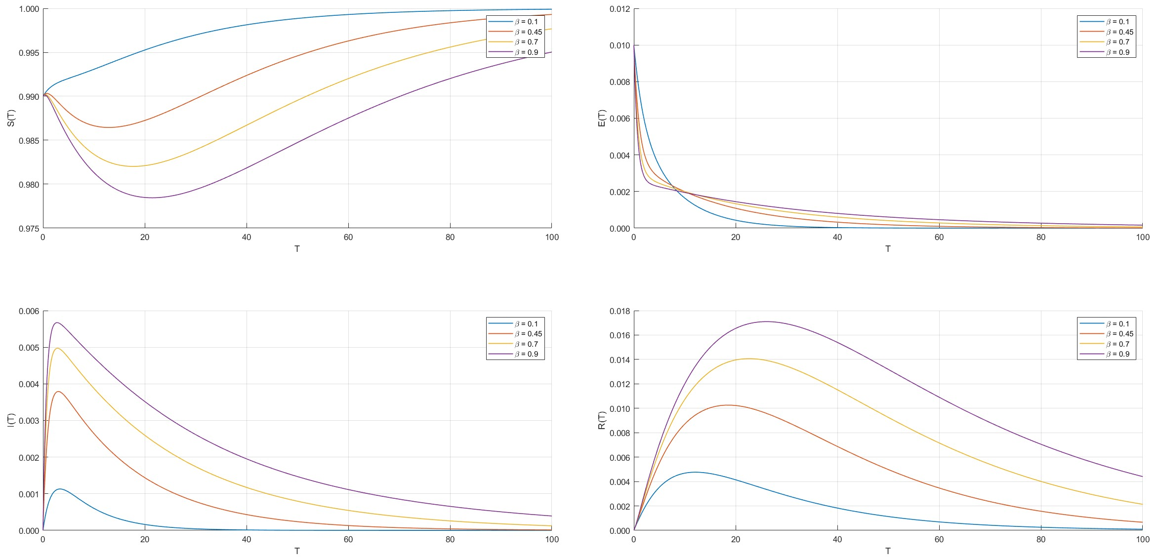
As shown in Figure 6, the curves for S(t), I(t), and R(t) differ more markedly across the examined β values than those for E(t). As β increases, the short-term peak of the infected proportion rises, while the decline in the susceptible proportion and the variation in the recovered proportion become more pronounced. Despite these short-term differences, S(t) ultimately approaches 1 and E(t), I(t), and R(t) approach 0 in all cases.
(3) Effect of γ. The parameter γ is the transition rate from the infected to the recovered state. The values γ = 0.1, 0.25, 0.7, and 0.9 are tested separately, and their effects on schedule-risk propagation are shown in Figure 7.
Figure 7.
Effects of γ on schedule-risk propagation.
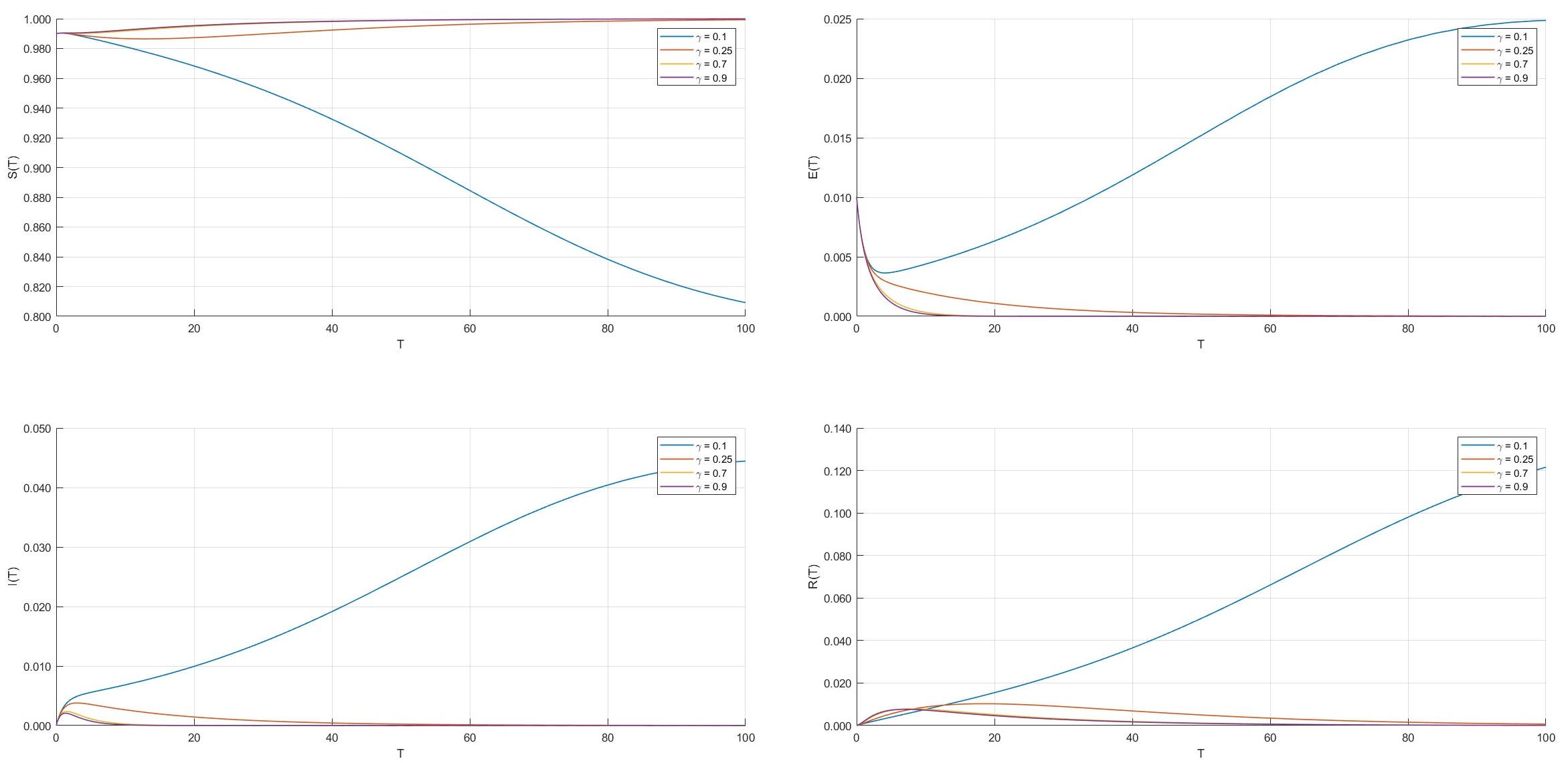
As shown in Figure 7, when γ = 0.25, 0.7, or 0.9, the state proportions exhibit different short-term responses, but S(t) ultimately approaches 1 and E(t), I(t), and R(t) approach 0. When γ decreases to 0.1, S(t) declines markedly, and the exposed and infected proportions remain nonzero near the end of the simulation.
(4) Effect of μ. The parameter μ is the transition rate from the recovered to the susceptible state. The values μ = 0.05, 0.3, 0.7, and 0.9 are tested separately, and their effects on schedule-risk propagation are shown in Figure 8.
Figure 8.
Effects of μ on schedule-risk propagation.
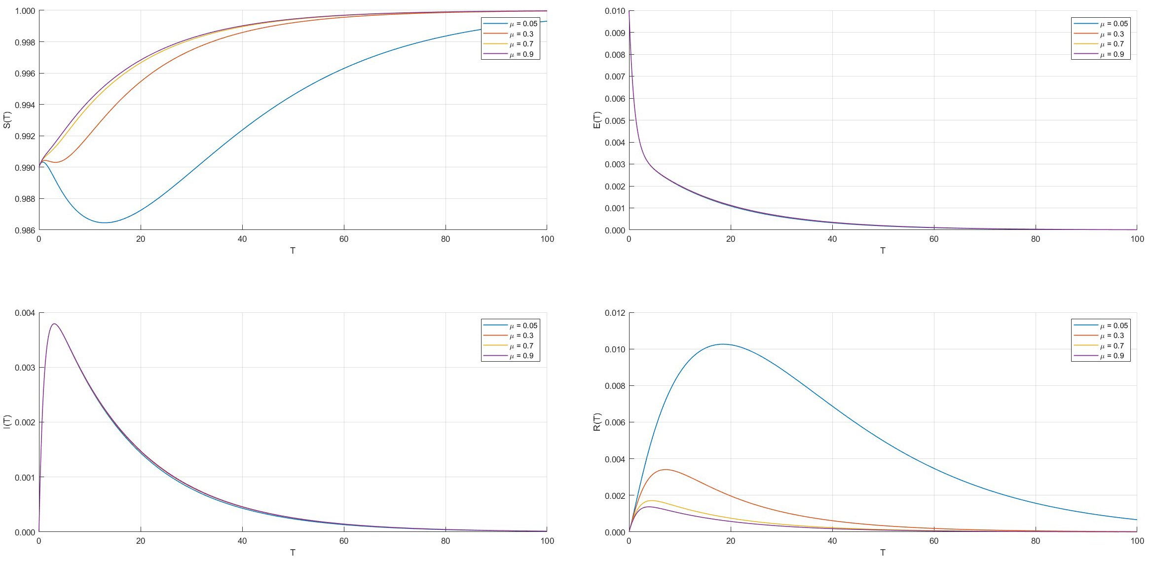
As shown in Figure 8, the E(t) and I(t) curves are similar across the examined μ values, whereas the S(t) and R(t) curves differ more markedly in their short-term amplitudes, recovered-state peaks, and decay processes. As μ increases, the recovered proportion reaches a lower peak and then declines more rapidly. In all scenarios, S(t) ultimately approaches 1, while E(t), I(t), and R(t) approach 0.
In Figure 5, Figure 6, Figure 7 and Figure 8, one parameter was varied at a time, with all other parameters held at their values in the baseline scenario in Figure 4. To complement the trajectory comparisons, the local relative sensitivity of the propagation threshold h to each parameter p was calculated from Equation (6) as . At the baseline, the sensitivities for α, β, γ, and μ were −1.000, −0.308, 0.625, and 0, respectively. Among these four parameters, α had the largest local effect on h for an equal percentage change. The zero sensitivity to μ reflects its absence from the threshold expression; Figure 8 shows that varying μ can still change the state trajectories.
6. Discussion
The foregoing results reveal the evolution of state fractions across threshold scenarios and parameter settings. This section further interprets the mechanisms behind such behaviors and their managerial implications, covering the threshold scenarios in Section 5.1 and the parameter comparisons in Section 5.2.
6.1. Risk Evolution Under Threshold Constraints
Section 5.1 shows that the two parameter combinations produce persistent-risk and risk-dissipation trajectories, respectively. In the h < 1 scenario, the exposed and infected proportions approach nonzero levels, which indicates a balance between risk propagation and mitigation in terms of state proportions rather than unbounded risk accumulation. By contrast, in the h ≥ 1 scenario, the exposed and infected proportions approach zero, indicating that risks cannot persist under the given parameter configuration.
Section 5.2 further shows that parameter adjustments can shift the system across the critical boundary even when the baseline scenario in Figure 4 satisfies h ≥ 1. Increasing α to 0.7 yields h ≈ 0.83, and reducing γ to 0.1 yields h ≈ 0.80; both cases enter the h < 1 region. By contrast, the examined variations in β and μ do not alter the ultimate risk-dissipation outcome. Parameter effects should therefore be evaluated from two dimensions: short-term differences among state curves and changes in the threshold condition; a mechanism should not be considered unimportant merely because the final states are similar. In practice, even a disruption that eventually resolves may warrant attention if it overlaps with a planned installation window or uses up the available schedule float. The model threshold distinguishes propagation regimes under the assumed parameters; project-specific alert levels would need to be established using schedule and disruption records.
6.2. Propagation Control and Latent-Risk Treatment
The propagation rate α determines the intensity with which infection risks generate new disruptions in susceptible processes. The more pronounced variations in the exposed and infected proportions at higher α values in Figure 5 are consistent with the persistent-risk scenario in Section 5.1. This consistency supports reducing propagation intensity as a means of limiting risk diffusion in the model. In practice, a fabrication delay can reduce the time available for transportation and lead to waiting at the planned lifting stage. This example illustrates how activity dependencies can transmit schedule disruptions. The model captures the aggregate effect of such interactions through αSI.
The exposure-to-infection rate β governs the development of existing latent disruptions into manifest abnormalities. Exposed nodes may enter the infected state at rate β or return directly to the susceptible state at rate η. They may also enter the recovered state directly at rate δ, so latent risks do not necessarily become manifest. Increasing β accelerates the flow from exposure to infection and shortens the average exposure duration, while the resulting increase in infected nodes can generate new exposed nodes. This mechanism helps explain the relatively limited variation in E(t) in Figure 6. Within the examined range, h remains greater than 1 even when β = 0.9, so variations in β do not move the system into the persistent-risk region. Before installation is disrupted, project teams can compare expected component dispatch and arrival times with the planned lifting window to identify activities whose schedule buffers are being depleted. Restoring the original delivery plan may resolve the immediate issue, whereas a confirmed backup arrangement may also provide temporary protection against a similar disruption; these are practical interpretations of the two pathways in the model, and their effectiveness depends on project conditions.
6.3. Recovery and Maintenance of Protection
The recovery rate γ affects both the recovery of infected nodes and whether the system satisfies the condition for risk dissipation. In Figure 7, γ = 0.25, 0.7, and 0.9 all lead ultimately to the risk-free state, although they may produce different risk peaks, durations, and cumulative effects. When γ decreases to 0.1, h ≈ 0.80 and risks may persist. The dependence on γ is consistent with the risk-dissipation scenario under stronger mitigation in Section 5.1.
The protection-loss rate μ directly governs the transition from the recovered state back to the susceptible state; a higher μ implies more rapid loss of protection. In Figure 8, its principal effect is to redistribute nodes between the susceptible and recovered states, with relatively limited effects on the exposed and infected proportions in these risk-dissipation scenarios. Faster loss of protection can reduce the number of temporarily protected nodes and leave more nodes susceptible to renewed disruption. If a component shortage interrupts lifting, project teams can assess how to resume the affected operation and then check whether any backup arrangement remains available for subsequent operations. The simulations use hypothetical parameters and report activity-state proportions, so they cannot quantify how much time these measures would save; that assessment requires actual stoppage records and an analysis of their effects on the critical path and project milestones.
7. Conclusions
Schedule risks in prefabricated construction originate from activity interactions and cover aggregate schedule deviations as well as the emergence, spread, mitigation and recurrence of disruptions. This study extends the analytical focus from overall schedule performance to activity-level risk states and their transitions. A SEIRS model is used to describe the dynamics of susceptible, exposed, infected, and recovered states, derive equilibrium points and the propagation threshold, and examine propagation behavior under alternative numerical scenarios. The main conclusions are summarized below.
(1) Persistent schedule-risk propagation is governed by a threshold condition. When h < 1, the model admits a positive equilibrium, and the simulations show that the exposed and infected proportions approach nonzero levels, establishing a dynamic balance between risk propagation and mitigation. When h ≥ 1, risks dissipate under the specified scenarios and the system approaches the risk-free equilibrium. Thus, h = 1 represents the critical boundary between these two regimes.
(2) Changes in the propagation and recovery rates can alter risk-evolution outcomes. Under the baseline parameters, increasing α to 0.7 yields h ≈ 0.83, while reducing γ to 0.1 yields h ≈ 0.80; both cases enter the parameter region that permits persistent nonzero risks. These findings highlight the importance of limiting propagation and maintaining adequate recovery capacity. Within the examined range and with the other parameters fixed at their baseline values, variations in β affect risk manifestation but do not shift the model into the persistent-risk regime.
(3) Risk mitigation and the maintenance of protection play distinct roles. The model allows exposed nodes to return directly to the susceptible state or enter the recovered state before risks become manifest. Thus, latent disruptions do not necessarily develop into infection risks. Recovered nodes may revert to the susceptible state when protective measures fail. In the risk-dissipation scenarios examined here, μ mainly affects the susceptible and recovered proportions, with relatively limited effects on the exposed and infected proportions. Schedule-risk management should therefore integrate early disruption detection, timely intervention after risk manifestation, and sustained protection after recovery.
This study provides a theoretical framework for understanding schedule risks in prefabricated construction from the perspective of risk-state transitions, but several limitations remain. First, the numerical simulations use hypothetical initial conditions and parameters that have not been calibrated or independently validated with project data. Second, the risk-state proportions have not yet been quantitatively linked to activity delays, critical-path adjustments, or project-completion deviations. Third, the parameter sweeps varied one parameter at a time, and the quantitative sensitivity comparison was limited to the propagation threshold near the selected baseline. The robustness of the simulated trajectories and the relative parameter effects across alternative baseline configurations or under joint parameter variation was not assessed. Future research may integrate component-production, transportation, installation, and risk-response records to improve state classification and parameter estimation. Linking the propagation model to activity-level schedule analysis would further enhance its practical applicability.
Author Contributions
Writing—original draft preparation, methodology, formal analysis, validation, visualization, Y.Y.; Conceptualization, writing—review and editing, data curation, Q.L.; All authors have read and agreed to the published version of the manuscript.
Funding
This research was supported by the National Natural Science Foundation of China (Grant No. 52578373).
Institutional Review Board Statement
Not applicable.
Informed Consent Statement
Not applicable.
Data Availability Statement
The raw data supporting the conclusions of this article will be made available by the authors on request.
Conflicts of Interest
The authors declare no conflicts of interest.
References
- Zhao, Y.; Chen, W.; Yang, Z.; Li, Z.; Wang, Y. Analysis on Risk Factors Related Delay in PCPs. Eng. Constr. Archit. Manag. 2022, 30, 4609–4644. [Google Scholar] [CrossRef] [Scilit]
- Shen, K.; Cheng, C.; Li, X.; Zhang, Z. Environmental Cost-Benefit Analysis of Prefabricated Public Housing in Beijing. Sustainability 2019, 11, 207. [Google Scholar] [CrossRef] [Scilit]
- Fan, C.; Binchao, D.; Yin, Y. Hierarchical Structure and Transfer Mechanism to Assess the Scheduling-Related Risk in Construction of Prefabricated Buildings: An Integrated ISM–MICMAC Approach. Eng. Constr. Archit. Manag. 2022, 30, 2991–3013. [Google Scholar] [CrossRef] [Scilit]
- Li, Z.; Zhang, S.; Meng, Q.; Hu, X. Barriers to the Development of Prefabricated Buildings in China: A News Coverage Analysis. Eng. Constr. Archit. Manag. 2020, 28, 2884–2903. [Google Scholar] [CrossRef] [Scilit]
- Dan, Y.; Liu, G. Integrated Scheduling Optimization of Production and Transportation for Precast Component with Delivery Time Window. Eng. Constr. Archit. Manag. 2023, 31, 3335–3355. [Google Scholar] [CrossRef] [Scilit]
- Liu, Y.; Chang, R.-D.; Zuo, J.; Xiong, F.; Dong, N. What Leads to the High Capital Cost of Prefabricated Construction in China: Perspectives of Stakeholders. Eng. Constr. Archit. Manag. 2022, 30, 805–832. [Google Scholar] [CrossRef] [Scilit]
- Xu, Z.; Liang, Y.; Lu, H.; Kong, W.; Wu, G. An Approach for Monitoring Prefabricated Building Construction Based on Feature Extraction and Point Cloud Segmentation. Eng. Constr. Archit. Manag. 2022, 30, 5302–5332. [Google Scholar] [CrossRef] [Scilit]
- Song, L.; Li, H.; Deng, Y.; Li, C. Understanding Safety Performance of Prefabricated Construction Based on Complex Network Theory. Appl. Sci. 2022, 12, 4308. [Google Scholar] [CrossRef] [Scilit]
- Çevikbaş, M.; Okudan, O.; Işık, Z. New Delay-Analysis Method Using Modified Schedule and Modified Updated Schedule for Construction Projects. J. Constr. Eng. Manag. 2022, 148, 04022119. [Google Scholar] [CrossRef] [Scilit]
- Xie, L.; Wu, S.; Chen, Y.; Chang, R.; Chen, X. A Case-Based Reasoning Approach for Solving Schedule Delay Problems in Prefabricated Construction Projects. Autom. Constr. 2023, 154, 105028. [Google Scholar] [CrossRef] [Scilit]
- Abdul Nabi, M.; El-Adaway, I.H. Understanding the Key Risks Affecting Cost and Schedule Performance of Modular Construction Projects. J. Manag. Eng. 2021, 37, 04021023. [Google Scholar] [CrossRef] [Scilit]
- Cho, K.; Ahn, S.; Park, K.; Kim, T.W. Schedule Delay Leading Indicators in Precast Concrete Construction Projects: Qualitative Comparative Analysis of Korean Cases. J. Manag. Eng. 2021, 37, 04021024. [Google Scholar] [CrossRef] [Scilit]
- Li, C.Z.; Hong, J.; Xue, F.; Shen, G.Q.; Xu, X.; Mok, M.K. Schedule Risks in Prefabrication Housing Production in Hong Kong: A Social Network Analysis. J. Clean. Prod. 2016, 134, 482–494. [Google Scholar] [CrossRef] [Scilit]
- Li, C.Z.; Hong, J.; Fan, C.; Xu, X.; Shen, G.Q. Schedule Delay Analysis of Prefabricated Housing Production: A Hybrid Dynamic Approach. J. Clean. Prod. 2018, 195, 1533–1545. [Google Scholar] [CrossRef] [Scilit]
- Abdul Nabi, M.; El-Adaway, I.H. A Proactive Risk Assessment Framework to Maximize Schedule Benefits of Modularization in Construction Projects. J. Constr. Eng. Manag. 2022, 148, 04022052. [Google Scholar] [CrossRef] [Scilit]
- Rezakhani, P. Project Scheduling and Performance Prediction: A Fuzzy-Bayesian Network Approach. Eng. Constr. Archit. Manag. 2021, 29, 2233–2244. [Google Scholar] [CrossRef] [Scilit]
- He, Z.; Huang, D.; Fang, J. Social Stability Risk Diffusion of Large Complex Engineering Projects Based on an Improved SIR Model: A Simulation Research on Complex Networks. Complexity 2021, 2021, 7998655. [Google Scholar] [CrossRef] [Scilit]
- Xu, J.; Zhu, J.; Xie, J. Study on the Evolution of Risk Contagion in Urban River Ecological Management Projects Based on SEIRS. Water 2023, 15, 2622. [Google Scholar] [CrossRef] [Scilit]
- Zhang, Y.; Tai, S.; Zhang, D.; Wu, L. How to Promote the Diffusion of Green Behavior among Contractors? Analysis and Simulation Using the SIR Model. J. Environ. Manag. 2023, 335, 117555. [Google Scholar] [CrossRef] [Scilit] [PubMed]
- Jia, J.; Xiao, J. Stability Analysis of a Disease Resistance SEIRS Model with Nonlinear Incidence Rate. Adv. Differ. Equ. 2018, 2018, 75. [Google Scholar] [CrossRef] [Scilit]

Disclaimer/Publisher’s Note: The statements, opinions and data contained in all publications are solely those of the individual author(s) and contributor(s) and not of MDPI and/or the editor(s). MDPI and/or the editor(s) disclaim responsibility for any injury to people or property resulting from any ideas, methods, instructions or products referred to in the content. |
© 2026 by the authors. Licensee MDPI, Basel, Switzerland. This article is an open access article distributed under the terms and conditions of the Creative Commons Attribution (CC BY) license.