


Abstract
Thermally activated building systems (TABS) shift energy demand away from grid peaks, yet retrofitted buildings often retain heterogeneous slabs, unlike the homogeneous slabs assumed in most studies. This study aims (i) to document compliance with the LEED v5 Grid Harmonization credit at Apolonio Morales 29, an office building in Madrid certified in 2025 with the highest score worldwide for this version; and (ii) to compare six slab typologies through adiabatic simulations with fixed operating parameters. Measurements show winter thermal peak-demand reductions of up to 90%, with a median 15 h reduced-demand period on 126 of 129 winter working days; simulated behavior was checked for consistency with these data. Composition mainly determined heat distribution between floors (inter-floor air-temperature gap of 1.5–1.6 °C in heterogeneous versus ≈ 0.7 °C in homogeneous slabs), whereas pipe depth and intervening mass determined accumulated demand (up to +82%). Heterogeneous slabs, like the case study, suit directional heating and a single nightly charging window; homogeneous slabs can serve two floors from one circuit at higher demand. Sensitivity analyses show relative demand and temperature patterns persist when infiltration or supply temperature change, whereas absolute demand and cycle durations do not, supporting relative comparisons for design and control.
1. Introduction
Thermally Activated Building Systems (TABS) are heating and cooling systems integrated into the structural mass of a building, capable of storing and releasing thermal energy over time by exploiting the thermal inertia of construction elements. Their usefulness depends jointly on their physical integration within the structure and on the control strategy applied to them. In offices and other buildings with restricted occupancy schedules, TABS are typically preheated or precooled overnight, shifting energy production to off-peak hours and reducing daytime peak loads [1,2]. Because the slab itself acts as the storage medium, TABS are natural candidates for building energy flexibility: predictive control allows buildings to harness the flexibility available in their passive thermal mass [3], and a recent systematic review of residential demand-side management identified load shifting as the dominant flexibility type [4].
The combination of TABS with geothermal heat pumps has been described as favorable when approached holistically [2,5], and model predictive control (MPC) has been proposed to optimize operation in hybrid GEOTABS buildings (TABS supplied by geothermal heat pumps) [5]. Because of their large thermal inertia, TABS are difficult to control, and a substantial body of literature addresses their control, simulation, and optimization. Early work established the control concepts and design guidance: Gwerder et al. [6] addressed the control of TABS, Tödtli et al. [7] published the TABS-Control book, and Lehmann et al. [8] linked energy efficiency to control strategy, hydronic circuit topology, and generation system. Kalz [9] reported heating and cooling concepts combining environmental energy and TABS for low-energy buildings. Reviews of TABS simulation and control [10], of thermal mass activation for thermal comfort, peak shifting, and shaving [11], and of the combination of thermal energy storage with buildings [12] consolidate this knowledge. Arteconi et al. [13] analyzed TABS control strategies under demand-side management mechanisms, and Lim et al. [14] developed operational guidelines from heating and cooling load characteristics.
More recent work has focused on predictive and learning-based control. Cupeiro Figueroa et al. [5] reviewed MPC formulations with a focus on hybrid GEOTABS buildings. Yang et al. [15] compared white-box, gray-box, and black-box MPC strategies with rule-based control in a TABS with large energy flexibility, reporting that MPC increased load-shifting cost savings by 30% to 50%. Liu et al. [16] applied an economic MPC to the TABS of a near-zero energy building in Tianjin and obtained a lower energy price cost than with rule-based control, and Hepf et al. [17] showed, with a validated simulation model, that a weather predictive control strategy can improve thermal comfort in an office building with TABS in Munich without increasing energy demand. Learning-based control has also been implemented in real buildings: Silvestri et al. [18] implemented a deep reinforcement learning controller in the TABS of a real building and improved indoor temperature control by 68% relative to the best-performing rule-based controller during a two-month cooling season, without increasing energy consumption. Kathirgamanathan et al. [3] reviewed data-driven predictive control for building energy flexibility, and Sharifi et al. [19] proposed a heuristic algorithm for optimal load splitting in hybrid TABS.
These studies mostly address purpose-designed systems. As recalled in a recent experimental validation in a passive office building [20], the hourly method of ISO 11855-4 describes the slab with one-dimensional heat transfer and a homogeneous temperature distribution in the horizontal direction. A recent review of TABS [21] analyzes system and fluid configurations (speed, temperature, and mass flow rate) in roofs, walls, and floors, and identifies gaps in the literature. Most of this literature assumes a homogeneous slab with embedded pipes, also known as concrete core activation (CCA), consistent with new-construction practice. However, considerably less evidence exists on TABS behavior in existing buildings, where conserving the original structure may result in heterogeneous rather than homogeneous slabs. The available contributions address related aspects: De Saulles [22] discussed the utilization of thermal mass in nonresidential buildings; Xu et al. [23] studied active hollow core slabs that use low-energy sources; De Pereda Fernández described the principles and cases of integration of thermoactive systems [24] and a model of action for improving energy efficiency in the comprehensive rehabilitation of a protected building for offices in Madrid, based on geothermal energy and thermoactive structures [25]; Reilly and Kinnane [26] assessed the impact of thermal mass on building energy consumption; and the authors’ earlier work on the case-study building addressed its control and monitoring [27] and its energy diagnosis [28]. In particular, how slab composition and pipe position affect thermal storage and discharge dynamics, and, consequently, the control strategy needed to shift energy demand, remains insufficiently investigated.
At the same time, European regulation on building decarbonization explicitly addresses existing buildings: the recast Energy Performance of Buildings Directive [29] includes provisions on existing buildings, zero-emission buildings and the smart readiness of buildings, and sustainability certification schemes are increasingly rewarding demand-side flexibility: the LEED v5 for Operations and Maintenance (O+M): Existing Buildings rating system introduces the “Grid Harmonization” credit under the Energy and Atmosphere category, crediting on-site thermal and/or electric energy storage capable of shifting demand away from grid peaks [30]. The Grid Harmonization credit is not used solely as a certification indicator, but also as a framework for evaluating, through operational data, the building’s actual capacity to shift demand. TABS-equipped buildings are natural candidates for this credit, since the slab itself can act as the storage medium, but demonstrating and interpreting this behavior in a real, heterogeneous, retrofitted structure requires linking site monitoring data with an understanding of how the specific slab composition governs thermal storage. The credit has evolved across LEED v5 editions. Initially named Grid Harmonization (1–2 points) in the September 2023 O+M beta [30], its requirements were incorporated into the Energy and Atmosphere credits (EAc) EAc4 Peak Load Reduction Performance (electric or thermal demand reduction) and EAc6 Peak Load Management in April 2025 [31], both retained in November 2025 [32]. The equivalent credit in LEED v5 Building Design and Construction (BD+C) is Grid Interactive (1–2 points) [33].
According to the U.S. Green Building Council (USGBC) public project directory [34], 32 buildings had been certified under LEED v5 O+M: Existing Buildings as of October 2026, and 12 (37.5%) earned points in the Grid Harmonization credit. Five obtained the maximum of two points: the International Commerce Centre in Hong Kong, the Xfinity Mobile Arena in Philadelphia, the Empire State Building in New York, Taipei 101, and the case-study building of this paper, Apolonio Morales 29 in Madrid. The publicly available directory descriptions of these buildings highlight general energy-efficiency measures but do not specify how the credit was achieved. Furthermore, to the authors’ knowledge, peer-reviewed studies documenting measured performance under LEED v5 remain limited, as the rating system was introduced only in 2025 [34].
This study addresses this gap by providing empirical evidence on the Grid Harmonization credit through monitoring data from Apolonio Morales 29, a Madrid office building equipped with a heterogeneous TABS system that achieved LEED v5 O+M Platinum certification on 8 August 2025 under the beta version of the rating system with a world-record score of 96/110 [35,36,37]. Specifically, it documents the building’s measured Grid Harmonization performance and, through a parametric numerical study of six slab typologies, examines how slab composition and pipe position shape thermal storage and discharge dynamics, using the real building as a consistency reference rather than as a validation case. It uses the typology-specific recharge dynamics from the simulation to examine whether the intrinsic thermal response associated with different slab typologies can explain differences in TABS thermal storage and discharge dynamics and, consequently, inform the selection of control strategies aimed at reducing peak demand. Because the parametric model was deliberately built under different boundary and control conditions to isolate the effect of slab composition, the comparison is a qualitative, pattern-level consistency analysis, with its methodological limits stated explicitly rather than absorbed into the conclusions. It is not intended to reproduce or validate the building’s measured demand: the simulated behavior of the slab is only checked for consistency with the real-building data, which provides a reference for interpreting the comparison between typologies.
Based on this framework, the main contributions of this paper are therefore: (i) to document, using operational data, the peak-demand reduction achieved by a retrofitted building equipped with TABS; (ii) to quantify, through a parametric study complemented by sensitivity analyses, the influence of slab configuration and pipe position on thermal dynamics; and (iii) to examine how these dynamics relate to the night-charging strategy of the real building and what they imply for control strategies tailored to different slab designs.
2. Materials and Methods
2.1. Case Study Building and Monitoring System
The case study is an 803 m2 office building, Apolonio Morales 29, in Madrid, Spain (Figure 1), comprehensively retrofitted between 2007 and 2009 in both envelope and energy systems, combining passive strategies (enhanced insulation, airtightness, solar control and daylighting) with active systems supplied by renewable and geothermal sources [24,25,27,28]. The characteristics of the envelope, ventilation and internal loads that set the baseline thermal load managed by the TABS are summarized in Table 1.
Figure 1.
Apolonio Morales 29, Madrid, Spain. 2010, Fernández Molina Obras y Servicios S.A.
Table 1.
Main characteristics of the case-study building (Apolonio Morales 29). Source: ASHRAE Level 2 energy audit of the building (ENERES technical report, unpublished). 2025, Fernández Molina Obras y Servicios S.A.
During the retrofit, 95% of the original structure was preserved to exploit its thermoactive potential. The preexisting slab, composed of double reinforced-concrete joists, hollow clay blocks and a concrete topping, was thermally activated by embedding water circulation pipes under an additional 7 cm cement mortar layer (Figure 2), and is supplied by two geothermal water-to-water heat pumps [24,25,27,28].
Figure 2.
Thermal mass activation. Floor section. Dimension arrows indicate the thickness of each individual slab layer. Apolonio Morales 29, Madrid, Spain. Created by the authors.
The Building Management System (BMS) regulates supply-water temperature and indoor setpoints according to a scheduled day/night logic: during nighttime hours (00:00–08:00), heat pumps charge the slabs applying a shifted setpoint (+1 °C in winter, −1 °C in summer) to maximize thermal storage; during occupied hours (08:00–19:00) an auxiliary Air Handling Unit (AHU) maintains indoor air quality and supplements the TABS in meeting the building’s heating and cooling demand. The AHU operates only during the occupied hours (08:00–19:00) and cleaning hours (06:00–08:00); between 19:00 and 24:00 it is switched off, while the TABS keep operating according to the parameters of the daytime band. The TABS provide the primary radiant conditioning at standard comfort setpoints, resulting in a hybrid configuration consistent with load-splitting strategies for combined TABS/auxiliary systems [19,27,28]. The monitoring infrastructure includes, among other devices, an outdoor temperature and humidity sensor, six indoor temperature and humidity sensors (two per floor), an electrical analyzer (three-phase energy meter) dedicated to the heating, ventilation, and air-conditioning (HVAC) system, and a Kamstrup Multical 403 thermal energy meter on the heat-pump circuit (Table 2; Figure 3), all logged at 10 min intervals. On each floor, two thermostats measure indoor air temperature, and the BMS regulates TABS operation by comparing their average value with predefined daytime and nighttime setpoints [27,28].
Table 2.
Measured variables, monitoring devices, and technical specifications of the sensors installed at Apolonio Morales 29 and used in this study.
Figure 3.
Electrical analyzer ((left); label in Spanish: “analizador de redes,” i.e., network analyzer) and thermal energy meter for flow rate and temperature (right) installed at Apolonio Morales 29, Madrid, Spain. 2020, Fernández Molina Obras y Servicios S.A.
2.2. LEED v5 Grid Harmonization Assessment (Real, Measured Data)
As discussed in the Introduction, the “Grid Harmonization” credit has evolved across LEED v5 editions. Since Apolonio Morales 29 was certified on 8 August 2025 under the LEED v5 O+M beta rating system [34], this study adopts the “Grid Harmonization” designation and the corresponding requirements applicable to the building’s certification.
Compliance with the LEED v5 O+M “Grid Harmonization” credit, Option 2 (“Thermal and/or Electric Energy Storage”), Criterion 3 (“Peak electric demand reduction”), was assessed using two independent, real data sources: (i) monthly electricity billing records for 2023 and 2024, disaggregated by the six periods of the Spanish 3.0TD tariff (P1, most expensive, to P6, cheapest, off-peak); and (ii) Building Management System (BMS) data on electrical and thermal demand for representative winter and summer days in 2024, complemented by the complete hourly series of 2023 and 2024 to test the representativeness of the winter days (Section 3.1).
Following Option 2 (Thermal and/or Electric Energy Storage), Criterion 3, of the LEED v5 O+M beta, the credit requires that storage reduce peak demand by at least 10% (1 point) or 20% (2 points), with the reduction sustained for at least two hours for electricity and four hours for thermal energy [30], consistent with the measured-energy-performance principles set out in EN 15378-3 [38]. The reduction is quantified on BMS data against a counterfactual baseline, that is, the peak that a conventional fast-response system would have reached, since it would have to supply during the occupied hours the energy that the TABS store overnight. It is expressed as ΔP = (Pbase − Pmeas) / Pbase × 100, where Pmeas is the highest demand recorded during the occupied hours and Pbase = Pmeas + Pcharge, with Pcharge the additional nighttime demand of the heat pumps that charge the slabs, estimated as the difference between the nighttime and the daytime demand levels. The same definition is applied to electrical and thermal demand, in winter and in summer, and it is illustrated on representative winter and summer days.
To document compliance with the LEED v5 credit, both a winter and a summer scenario were analyzed. In summer, however, several concurrent factors, such as the support of the AHU for peak cooling, the overnight precooling of the slabs and the solar and internal gains, complicate the attribution of the reduction to the TABS and limit the direct application of the methodology. This paper therefore focuses on winter behavior, which is also the focus of the simulations.
To assess whether the representative days are typical, the complete hourly series of electrical and thermal demand for 2023 and 2024 was analyzed for winter working days, defined as Monday to Friday between December and February (129 days; public holidays were not excluded). For each day, the nighttime level is the mean demand between 00:00 and 08:00, and the reduced-demand period is the number of consecutive hours after 08:00 in which demand stays at least 20% below that level, which is the reduction required by the credit. For thermal demand, thresholds of 50% and 90% were also tested, and the heat delivered before and during the reduced-demand period was summed hour by hour. Days with a nighttime thermal level below 20 kW were considered days without nighttime charging.
Measurement Uncertainty
The uncertainty of the measured demand was assessed from the maximum permissible errors (MPEs) of the two meters in Table 2 and propagated to the reduction ΔP and to the reduced-demand durations. The electrical analyzer is an accuracy Class 1 active-energy meter, with an MPE of ±1.0% of the reading over most of its current range and ±1.5% at the lowest currents [39]; the larger value, e = 1.5%, was applied to every electrical reading. For the thermal energy meter, the MPE of the complete meter is the sum of the errors of the flow sensor (Ef), the temperature-sensor pair, and the calculator, and it increases at low flow rates and at small supply–return temperature differences [40]. For the flow sensor of Table 2, the maximum permissible error is limited to 5% [40], and the errors of the temperature-sensor pair and of the calculator cannot exceed 3.5% and 1.5%, respectively, within the rated operating range [40]; the complete meter therefore cannot exceed 5% + 3.5% + 1.5% = 10%, and this bound, e = 10%, was applied to every thermal reading.
Because all the quantities entering ΔP = Pcharge / Pbase are measured with the same meter, a common gain error cancels out. A conservative bound was nevertheless obtained by assuming that each reading involved, namely Pmeas and the nighttime and daytime levels from which Pcharge is obtained (Pnight and Pday), deviates by the full MPE, independently and in the least favorable direction: |δΔP| ≤ e·Pmeas·(Pnight + Pday + Pcharge) / Pbase2, with Pday = 0 when Pcharge is taken directly as the nighttime level, as on the representative summer day (Section 3.1). Since Pday ≤ Pmeas and Pnight ≤ Pbase, this bound never exceeds 2e·(1 − ΔP), with ΔP expressed as a fraction. The same MPEs were used to assess the reduced-demand durations: because each hourly value is compared with a fraction of the nighttime level of the same day, its classification can change only if its ratio to that level lies within about ±2e of the threshold ratio (0.8 for the 20% criterion).
2.3. Parametric Simulation of Slab Typologies (Simulated Data)
A dynamic thermal simulation study, developed in DesignBuilder v7.3.1.003 [41], whose simulation engine is EnergyPlus v9.4 [42], modeled six slab typologies under a simplified two-story geometry (two superimposed 10 m × 10 m × 3 m blocks, F1 and F2) and adiabatic envelope boundary conditions, designed to minimize external heat-transfer effects and isolate the influence of slab composition and pipe position. In the two-story geometry model, only the intermediate slab separating the two floor blocks (F1 and F2) was activated, as this configuration isolates the response of a single thermoactive element and enables a consistent comparison across the six slab typologies. Typologies 1–3 are heterogeneous (single or double joist with ceramic hollow block, pipe under a 7 or 4 cm cement mortar cover); typology 4 is homogeneous but shares typology 3’s cover and pipe position, isolating the base-material effect alone; typologies 5–6 are homogeneous concrete core activation (CCA) configurations, with the pipe at upper/mid or lower third depth, serving the upper (F2) or lower (F1) floor (Table 3, Figure 4). Material properties came from the Spanish Technical Building Code (CTE DB-HE) [43].
Table 3.
Simulated slab typologies (single-slab activation scenario). Created by the authors.
Figure 4.
Schematic cross-sections of the six simulated slab typologies (numbered 1–6), showing water-pipe position (not to scale). Typology 2 corresponds to the real case-study slab. Created by the authors.
Concrete fraction in typologies 1–3 (Table 3, Figure 4) is a volume fraction per unit plan area, referred to the total slab thickness and averaged over one repeating module (one joist group plus one adjoining hollow-block span), assuming a 60 cm hollow-block span and a 10 cm single joist (typology 1) or two 10 cm joists (20 cm combined, typologies 2–3). For typology 2, for example, the concrete comprises the 60 mm topping plus the two joists, which occupy 20 cm of every 80 cm module, over the 240 mm block depth: (60 + 240 × 0.25) / 380 = 32%.
The hydraulic configuration was kept identical for all slab typologies to isolate the effect of slab composition and pipe position. The hydronic system consisted of pipes with an internal diameter of 0.018 m, spaced 0.20 m apart, with a total length of 500 m per slab distributed across five circuits of 100 m each. The total water flow rate was fixed at 360 L/h per slab (72 L/h per circuit).
In the actual building, slab supply temperature setpoints vary with outdoor temperature, ranging from 30 to 45 °C in winter. A constant supply temperature of 30 °C, within the recommended heating range of 25–40 °C [44], was adopted for all typologies to ensure consistent boundary conditions. This approach allows differences in thermal response to be primarily attributed to slab composition and pipe position. The influence of the supply temperature was assessed with additional simulations at 35 and 40 °C (Section Sensitivity to the Infiltration Rate and the Supply Temperature).
In the real building, the air-temperature setpoints are scheduled and vary over the year within the comfort range (20.0–24.0 °C) of EN 16798-1:2019 [45]. During winter, the nighttime setpoint is maintained approximately 1 °C higher than the daytime setpoint, promoting overnight thermal charging of the slabs. In the simulation, a continuous control logic with a constant air-temperature setpoint of 20 °C was applied, the same controlled variable as in the real building. This value is a prescribed simulation condition and not a reproduction of the building’s schedule. It corresponds to the lower bound of the Category II operative temperature range for sedentary activity in the heating season (20.0–24.0 °C) of EN 16798-1:2019 [45] and matches the default heating setpoint for nonresidential buildings under Spanish energy regulations [46]. As the standard refers to the operative temperature while the controlled variable is the air temperature, the setpoint is used as a reference value and not as a compliance check. It was kept constant to avoid any control-induced effect on the charging dynamics, so that the intrinsic thermal response of each slab typology can be investigated without imposing scheduled charging periods.
A 672 h simulated period, from 18 December to 14 January, was selected as the coldest four-week period of the ESP_MADRID_IWEC weather file, ensuring pronounced heating demand and well-defined thermal charging and discharging cycles. The simulations used the International Weather for Energy Calculations (IWEC) climate file for Madrid [47,48], developed by ASHRAE from historical hourly weather records archived at the U.S. National Climatic Data Center. Over the selected period, the outdoor dry-bulb temperature ranges from −4.6 °C to 14.4 °C, while solar radiation varies substantially, reaching a maximum of 762 W/m2. However, solar radiation does not influence the simulation results, as the model consists of opaque, adiabatic surfaces.
Although the theoretical model was defined as an adiabatic block to minimize the influence of external boundary conditions, a controlled level of infiltration was introduced as the only heat-loss mechanism: a fully closed adiabatic model without internal gains has no heat-loss path, so after the initial transient, the demand would fall to zero and no recharge/discharge cycles could be observed. The infiltration is constant and uniform; it couples the zones to the outdoor temperature, and it provides a daily load cycle that is identical for all typologies. An infiltration rate of 0.2 air changes per hour (ACH) was adopted, consistent with the value adopted in the calibrated DesignBuilder model of the actual building (Apolonio Morales 29) developed within the research project [49]. In that model, infiltration and thermal mass were identified as the main parameters controlling indoor air temperature oscillations and adjusted to match simulated and measured hourly temperatures. Calibration errors remained within the limits specified in [49] (maximum normalized mean bias error, NMBE, of 4.6% and coefficient of variation of the root mean square error, CV (RMSE), of 5.0% across three typical summer weeks in 2022, against thresholds of 10% and 30%, respectively). A blower-door test was attempted in the case-study building but did not yield valid results, because the building is a single open-plan volume without airtight compartments and the available fans were too small. No valid blower-door test results are therefore available.
With no internal or solar gains in the model, infiltration is the sole thermal load and determines the heating demand imposed on the slabs.
In addition to cumulative heating demand, the analysis examined the recharge and discharge periods of each typology. The discharge period was defined as the interval during which heating demand remained zero (inactive) for more than four consecutive hours, consistent with the principle adopted in LEED v5 Grid Harmonization, Option 2, Criterion 3 [30]. For each typology, the preceding recharge period was defined as the interval between the first relevant heating-demand peak and the final peak preceding the discharge period. Recharge and discharge durations for each typology are taken as the median over all complete cycles identified. The first 120 h were excluded as a warm-up period, because the simulation starts from uniform initial temperatures; only the data after this period, which are more reliable, were analyzed (the first days can be seen in Appendix B, Figure A2).
2.4. Basis for Comparison and Methodological Limitations
The real (measured) and simulated data sets differ in several respects that preclude a direct, quantitative comparison and must be stated explicitly: (i) the real building is exposed to actual Madrid weather, solar radiation, occupancy and an auxiliary AHU, whereas the simulated model excludes solar radiation, occupancy and AHU interaction by design; (ii) the real building operates under a scheduled, asymmetric setpoint control logic, whereas the simulation applies a continuous, constant-setpoint logic specifically to expose the composition-driven thermal behavior, undistorted by any control strategy; (iii) the real data cover full calendar years 2023–2024, with monthly billing data and hourly BMS data, whereas the simulation covers a single representative 672 h winter period at hourly resolution. For these reasons, this paper does not attempt to reproduce or numerically validate the real building’s measured demand-reduction percentages using the simulated typologies. Instead, it uses (i) the structural correspondence between the real slab and simulated typology 2 as a consistency check of the simulated slab behavior, and (ii) the typology-specific recharge dynamics obtained under controlled simulation conditions, as the basis for comparing slab typologies.
The simulated geometry (two 10 × 10 × 3 m zones) is much smaller than the 803 m2 case-study building. With adiabatic external surfaces and infiltration as the sole thermal load, the thermal response is governed by the slab cross-section and by the zone volume-to-activated-area ratio (that is, the story height), not by the plan dimensions. Intensive and time-based indicators (demand per m2, temperatures and cycle durations) can therefore be examined for consistency with measured data, while building-specific effects such as envelope losses, perimeter zones, solar gains, the number of activated floors, the semibasement, the actual activated area and the spatial configuration remain outside the scope of the model. In particular, the simulated inter-floor temperature differences refer to an idealized two-story configuration with a single activated slab and are not a reproduction of the real building, where the lower floor is also affected by the floor below; they are therefore compared only among typologies, not with measured temperatures.
The constant infiltration rate and the constant supply temperature (Section 2.3) are modeling assumptions, not measured values. Their influence was assessed for typologies 2 and 5 (Section Sensitivity to the Infiltration Rate and the Supply Temperature). The simulated model was deliberately built with adiabatic surfaces and a fixed infiltration rate, in order to limit and control the external factors and to restrict the analysis to a pure comparison between slab typologies. Therefore, this is a relative rather than an absolute quantitative analysis, aimed at comparing slab typologies rather than establishing an energy balance of the charging period, which depends on the real building envelope. The 672 h period represents heating-dominated winter conditions; cycle durations under mid-season or cooling conditions were not simulated and may differ.
3. Results
3.1. Measured Grid Harmonization Performance at Apolonio Morales 29 (Real Data)
Table 4 summarizes annual electricity consumption by tariff-period group for 2023 and 2024. Off-peak period P6 concentrates approximately 52–53% of annual consumption in both years; the monthly distribution (Figure 5) shows this concentration is markedly stronger in winter months, when TABS night-charging dominates operation, than in summer, when the auxiliary AHU contributes more to daytime cooling.
Table 4.
Annual electricity consumption by tariff-period group. Source: electricity bills, Apolonio Morales 29, 2023–2024.
Figure 5.
Monthly electricity consumption by tariff-period group, 2024. Source: electricity bills, Apolonio Morales 29; LEED v5 Grid Harmonization report, 2025.
On the basis of hourly BMS data, a reduction in peak electrical demand exceeding 20% is sustained for more than two consecutive hours following the off-peak period (P6) in every month of the year, and for up to 14 consecutive hours in some months.
On a representative winter day (8 January 2024), the electrical demand remained at its nighttime level until about 10:00, beyond the programmed charging window (00:00–08:00). This may indicate that the slabs need about two hours beyond the programmed window to reach the daytime setpoint. Nighttime electrical demand exceeded daytime levels by approximately 10 kW on average, which corresponds to a reduction in daytime peak demand of at least 27% over a 14 h period (Figure 6a).
Figure 6.
Evolution of (a) peak electrical and (b) peak thermal demand throughout a typical winter day (8 January 2024) and a typical summer day (22 July 2024). The blue band is the night-charging window programmed in the BMS and the yellow band the occupied hours; the arrows above (a,b) show the recharge and reduced-demand periods of the winter day, the vertical dashed lines mark the end of the recharge period, and the dotted lines show the baselines of Table 5. Source: BMS of Apolonio Morales 29; LEED v5 Grid Harmonization report, 2025.
On a representative summer day (22 July 2024), the heat pumps and circulation pumps drew between 6 and 10 kW overnight to precool the slabs, and the daytime peak reached 30 kW; taking the overnight demand as 10 kW, the reduction relative to a conventional fast-response system is 25% (Figure 6a).
Thermal demand shows analogous reductions, from approximately 20% up to 100% in specific cases, sustained for four to fourteen consecutive hours after P6 and particularly in winter. In Figure 6b, positive values denote heat supplied to the building (winter) and negative values heat extracted from it (summer).
On the representative winter day, the thermal power dropped from 37 kW during the nighttime charging phase (programmed from 00:00 to 08:00, with the high level maintained until about 10:00) to 1–4 kW during the following 13 consecutive hours from 11:00 (14 h counting the transition hour from 10:00 to 11:00); with Pmeas taken as the upper residual value (4 kW), Pbase approaches the nighttime charging level (37 kW) and the reduction is 89% (reported as up to 90%).
On the representative summer day, the overnight precooling averaged about 10 kW of thermal power, and the daytime peak, which appeared around 12:30, reached approximately 21 kW of heat extracted; the reduction relative to a conventional fast-response system is therefore 32% (Figure 6b).
The shaded bands in Figure 6 mark the nighttime charging period programmed in the BMS (00:00–08:00, blue) and the occupied hours of the building (08:00–19:00, yellow) described in Section 2.1. On the winter day, the demand remains at its nighttime level until about 10:00, beyond the programmed window. The BMS data were logged at 10 min intervals (Table 2); the multi-day analysis below uses hourly means.
These results, summarized in Table 5, substantiate compliance with LEED v5 Grid Harmonization, Option 2, Criterion 3 (reduction of at least 20% for 2 points) [30], with the reductions calculated for the four cases against the baseline defined in Section 2.2.
Table 5.
Measured peak-demand reductions on the representative winter (8 January 2024) and summer (22 July 2024) days. Pmeas: highest demand during the occupied hours; Pbase = Pmeas + Pcharge; ΔP = (Pbase − Pmeas) / Pbase × 100. Sustained reduction: In winter, the duration corresponds to the reduced-demand period. In summer, it is assumed to last at least throughout the occupied hours (08:00–19:00), during which the AHU supports the preactivated TABS, and demand remains below Pmeas, corresponding to a minimum duration of 11 h. Source: BMS of Apolonio Morales 29; LEED v5 Grid Harmonization report, 2025.
The complete hourly series show that the representative winter day is typical (Figure 7; Appendix A, Figure A1 and Table A1). The electrical demand (Figure 7a) fell at least 20% below its nighttime level for at least 2 h after 08:00 on 128 of the 129 days (median 13 h, interquartile range, IQR, 10–15 h). Nighttime charging took place on 126 of the 129 winter working days. On these days, the thermal demand (Figure 7b) stayed at least 20% below the nighttime level for a median of 15 h after the charging window (IQR 13–16 h; range 6–16 h), well above the 4 h required by the credit; the 14 h of 8 January 2024 lies within the interquartile range, whereas the longest duration (16 h) exceeds the 14 h cited above from the credit report. A stricter threshold (demand at least 90% below the nighttime level) gives a median of 13 h (IQR 9–14 h), which is the criterion behind the 13 h of Table 5.
Figure 7.
Measured demand on the winter working days of 2023 and 2024. (a) Median and interquartile range of the hourly electrical power on the 129 winter working days, with 8 January 2024. (b) Same for the thermal power on the 126 charging days. The blue band is the night-charging window programmed in the BMS and the yellow band the occupied hours; the arrows show the recharge and reduced-demand periods for 8 January 2024 and as the median of the days, and the dashed vertical lines mark the end of the recharge period for 8 January 2024 (black) and for the median (colored). Source: BMS of Apolonio Morales 29.
The charging block ended at or before 08:00 on 49 of the 126 charging days but extended to 09:00 or later on 77 days (61%) and to 10:00 or later on 61 days (48%), as on the representative day (Figure A1b). A median of 95.1% (IQR 92.6–97.1%) of the daily thermal energy (357 kWh; IQR 299–403 kWh) was delivered before the reduced-demand period and only 4.9% (IQR 2.8–7.2%) during it, so that the heat pumps concentrate their output in the charging block while the building remains in operation.
Measurement uncertainty does not alter these results. With the bounds of Section Measurement Uncertainty (e = 1.5% for the electrical analyzer and 10% for the thermal energy meter), the reductions in Table 5 (27.9%, 25.0%, 89.2% and 32.1%) change by at most ±2.2 percentage points in the winter electrical case, ±0.6 in the summer electrical case, ±2.2 in the winter thermal case and ±4.4 in the summer thermal case, so that their lowest values (25.7%, 24.4%, 87.0% and 27.7%, respectively) remain above the 20% threshold of the credit. For any case to fall below this threshold, every reading would have to deviate by more than 5.4% for the electrical analyzer, 3.6 times the adopted bound, or more than 27% for the thermal energy meter. The reduced-demand durations obtained with the 20% criterion are also robust: daytime thermal demand (1–4 kW) lies far below the threshold of about 28 kW (80% of the median nighttime level of 35 kW; Table A1), so that only the transition hour at the end of the charging block can change classification, which is within the hourly resolution of the analysis. The electrical duration of an individual day can change when an afternoon peak approaches the threshold, as on 8 January 2024 (Figure 7a), and the durations obtained with the 90% criterion, whose threshold (about 3.5 kW) lies within the range of daytime thermal demand, should be regarded as indicative.
3.2. Simulated TABS Typology Performance
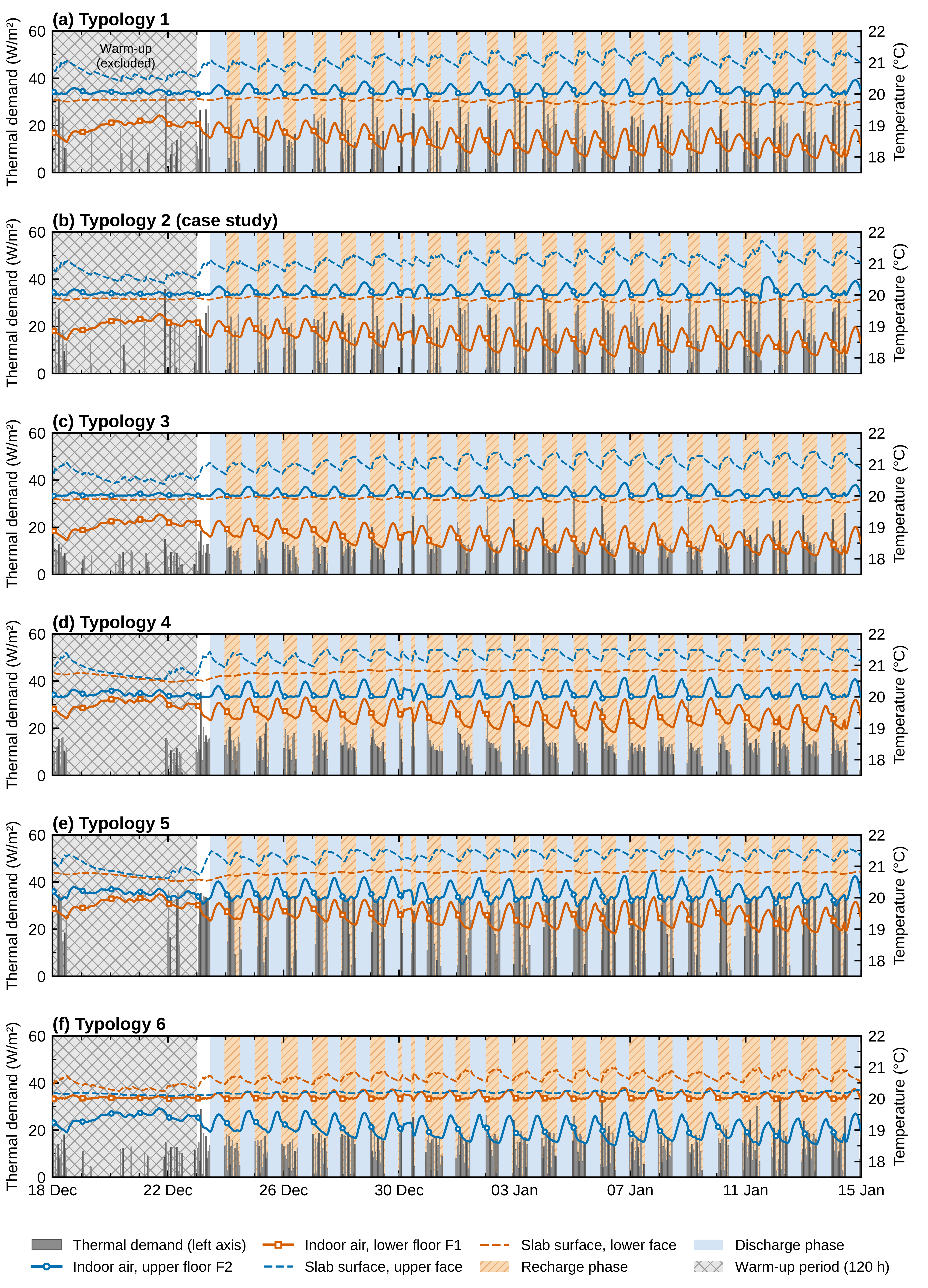
Figure 8 shows, for a representative 72 h window (31 December 00:00 to 3 January 00:00), the thermal power demand (gray bars, left axis), together with the indoor air temperature at the upper (F2) and lower (F1) floors (solid lines, right axis) and the surface temperatures of the upper and lower slab faces (dashed lines, right axis) for each of the six typologies. Air temperatures are zone-mean values (well-mixed assumption) and surface temperatures are area-averaged inside-face values of each side of the activated slab; they are model outputs and have no physical sensor location. The full 672 h series (18 December–14 January) is shown in Appendix B (Figure A2), and the hourly results of the six typologies are provided in Excel File S1 (Supplementary Materials).
Figure 8.
Thermal demand, indoor air temperature, and slab surface temperature of the six simulated typologies over a representative 72 h window (31 December 00:00 to 3 January 00:00), single-slab activation scenario. Source: Authors’ own simulations.
Parameters corresponding to the upper floor (F2) are shown in blue, while those corresponding to the lower floor (F1) are shown in orange (Figure 8). In the same figure, the recharge and discharge cycles described in Section 2.3 can be clearly observed. Table 6 reports, for the single-slab activation scenario, the accumulated heating demand, the recharge and discharge, for each of the six typologies defined in Table 3 (see also the schematic in Figure 4).
Across the six typologies, the three heterogeneous configurations (1–3) register the lowest accumulated demand (3.39–3.54 kWh/m2); homogeneous typology 5 (upper/mid-third pipe) shows substantially higher demand (6.19 kWh/m2), while typologies 4 (pipe under cover) and 6 (pipe at lower third) show values close to, but slightly higher than, those of the heterogeneous group (3.80–3.96 kWh/m2). The six typologies complete approximately one cycle per day (23–24 h; 1.00–1.04 cycles/day), with the daily active window occurring at the same climate-set hours for all typologies. What varies systematically is how that daily cycle is apportioned between the recharge (active) and discharge (inactive) phases.
Table 6.
Accumulated demand and recharge/discharge cycle timing, computed from the raw hourly simulation dataset (Excel File S1), by slab typology, single-slab activation scenario. Bold indicates the case-study slab (typology 2). Source: Authors’ own simulations.
The corresponding data in Table 6 quantify these differences using the recharge-to-discharge split. Doubling the joist count at fixed cover and pipe position (typology 1 → 2) leaves the split essentially unchanged (10.5 h/13.0 h vs. 10.0 h/13.0 h) and changes accumulated demand only marginally (3.45 → 3.54 kWh/m2, +2.6%). Reducing cover thickness by 3 cm (typology 2 → 3) shifts the split toward balance (12.0 h/12.0 h), while demand decreases slightly (3.54 → 3.39 kWh/m2, −4.2%). Replacing the heterogeneous base with a homogeneous slab at the same pipe position (typology 3 → 4) reverses this balance (13.0 h/10.0 h), accompanied by a 16.8% increase in cumulative demand (3.39 → 3.96 kWh/m2). Moving the pipe from 50 mm to 160–165 mm depth within the homogeneous slab (typology 4 → 5) leaves the recharge/discharge split close to balanced (12.0 h/12.0 h) while producing the largest single change in cumulative demand, an increase of 56.3% (3.96 → 6.19 kWh/m2). The transition from typology 5 → 6 combines a change in pipe depth with a change in the served floor (F2 to F1); the split remains close to balanced, while cumulative demand decreases by 38.6% (6.19 → 3.80 kWh/m2). Pipe depth, rather than the degree of material heterogeneity, therefore appears to have a stronger influence on cumulative demand than on the recharge/discharge balance itself, which stays comparatively close to an even split across most typologies (Section 2.3).
As Figure 8 shows, peak intensity within the recharge window follows a pattern related to pipe depth and cover thickness. Typologies 3, 4 and 6, whose pipes sit under a thinner cover or closer to their respective served surfaces, show more moderate median peaks (22.2–22.6 W/m2); typologies 1, 2 and 5, whose pipes sit under a thicker cover or deeper within the slab, show higher median peaks (30.9–33.6 W/m2).
Finally, Figure 9 shows a consistent pattern in both indoor air and slab surface temperature. For the heterogeneous group (typologies 1–3), the served floor (upper) is 1.5–1.6 °C warmer in terms of indoor air temperature and 1.2–1.3 °C warmer at the slab surface than the unserved floor (lower). Replacing the heterogeneous base with a homogeneous slab while keeping the pipe position and served floor unchanged (typology 3 → 4) nearly halves both temperature differences (air: 0.7 °C, −50%; surface: 0.5 °C, −56%). This indicates that material composition strongly affects heat distribution between the two floors. The lower thermal conductivity of the ceramic hollow blocks compared with concrete (λ = 0.6 W/m·K vs. 2.3 W/m·K) limits heat transfer toward the unserved floor in the heterogeneous configurations, whereas the homogeneous concrete slabs favor heat transfer toward the lower floor, thereby reducing the thermal gap between the two levels. A similar reduction is observed for typology 5 (air: −49%; surface: −53%), whereas the temperature difference reverses in typology 6, which serves the lower floor instead.
Figure 9.
Distribution of the slab surface temperature ((a): lower and upper faces) and of the indoor air temperature ((b): lower floor F1 and upper floor F2) across the six slab typologies; the dashed line marks the 20 °C setpoint and the diamonds the means. Source: Authors’ own simulations.
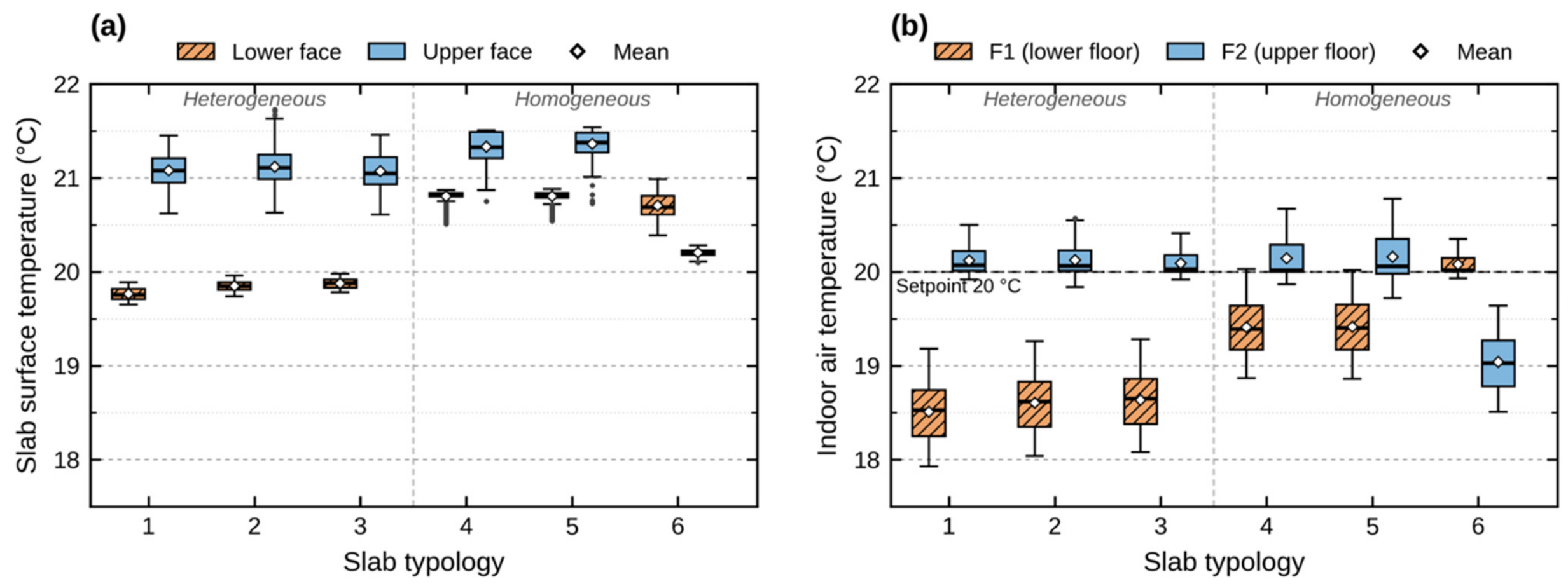
Sensitivity to the Infiltration Rate and the Supply Temperature
To test whether the comparison between typologies depends on the infiltration rate and the supply temperature fixed in the model, one typology was selected for each slab composition: typology 2 for the heterogeneous composition (the case study and the heterogeneous typology with the highest accumulated demand) and typology 5 for the homogeneous composition (the homogeneous typology with the highest accumulated demand). Both were simulated at 0.1 and 0.4 ACH (reference: 0.2 ACH) and at 35 and 40 °C (reference: 30 °C) (Table 7; full results in Appendix B, Table A2, and Excel Files S2 and S3). The infiltration rate scales absolute demand (−55% at 0.1 ACH; +130% in typology 2 and +122% in typology 5 at 0.4 ACH), but typology 5 demand remains 1.69–1.75 times that of typology 2, and the homogeneous slab maintains the smaller air-temperature difference between floors. Recharge and discharge durations do depend on the load (typology 2: 8.5/15.0 h, 10.0/13.0 h and 16.0/9.0 h at 0.1, 0.2 and 0.4 ACH), and at 0.4 ACH the upper-floor air temperature no longer holds the 20 °C setpoint, so durations should be compared only under identical boundary conditions.
Table 7.
Sensitivity of the accumulated demand, the median recharge and discharge periods and the air and slab-surface temperature differences between floors (F2−F1 and upper−lower face) to the infiltration rate and the supply temperature for typologies 2 and 5. The reference case (0.2 ACH and 30 °C) is highlighted in bold to distinguish the baseline simulation from the sensitivity scenarios; full results in Table A2 and Excel Files S2 and S3. Source: Authors’ own simulations.
The supply temperature changes the accumulated demand by less than 2.5% and leaves the temperature differences between floors unchanged; it mainly raises the peak demand (from 37 to 58 W/m2 in typology 2 and from 36 to 84 W/m2 in typology 5 between 30 and 40 °C), shortening the recharge by 1–3 h and lengthening the discharge by 1–1.5 h without altering their order between typologies.
4. Discussion
4.1. Thermal Energy Storage and Peak-Demand Reduction
Apolonio Morales 29 demonstrates, in full-scale operation, that a night-charging strategy applied to its heterogeneous slab can achieve substantial and sustained peak-demand reductions, including thermal-demand reductions of up to 90% (Section 3.1; baselines defined in Section 2.2). Independently, the parametric simulation shows that, among the six typologies studied, the heterogeneous configurations structurally equivalent to the real slab have the lowest accumulated demand of the set (Section 3.2). This lower demand should not be interpreted solely as evidence of higher thermal efficiency. Rather, it reflects how the amount of material between the pipe and the served surface, whether varied through pipe depth or through material composition, governs thermal response and heat-transfer dynamics.
The reductions in Table 5 were calculated with the same definition for the four cases, electrical and thermal demand in winter and in summer, which differ only in the size of Pmeas. In winter, no fast-response auxiliary system supports the TABS in covering peak heating demand, since the air handling unit acts as an auxiliary system for peak cooling in summer (ASHRAE Level 2 energy audit of the building). The heat stored overnight therefore supplies the daytime demand; Pmeas is residual (1–4 kW) and the baseline approaches the nighttime charging level (37 kW), which explains why the reduction in winter thermal demand is much higher than in the other cases.
Both pipe depth and material composition act, in fact, through this same underlying mechanism. Within each material group, a shallower pipe position is associated with a longer recharge phase, a shorter discharge phase, and lower accumulated demand: typology 3 shows this relative to typologies 1–2 within the heterogeneous group, as does typology 4 relative to typology 5 within the homogeneous group, where moving the pipe deeper (typology 4 → 5) raises accumulated demand by 56% and the median peak intensity from 22.3 to 33.6 W/m2 (Section 3.2). At a fixed pipe position, replacing the heterogeneous base with a homogeneous slab shows the opposite pattern, with a shorter recharge phase, a longer discharge phase, and lower accumulated demand for the heterogeneous configuration (typology 3 vs. 4). The greater pipe-to-surface distance and the larger amount of intervening thermal mass increase the thermal resistance between the circuit and the conditioned surface, potentially limiting heat transfer and requiring higher heating power to meet the same setpoint; this behavior is consistent with the thermal response reported by Velasco Gómez et al. [50]. Material composition also has a distinct effect on heat distribution: the air-temperature gap between served and unserved floors decreases by up to 50% in the corresponding homogeneous configuration (Figure 9), because the lower thermal conductivity of the ceramic hollow blocks limits heat transfer toward the unserved floor in heterogeneous slabs, whereas homogeneous slabs favor heat transfer toward the lower floor.
On the other hand, recharge and discharge durations do not divide cleanly along heterogeneous-versus-homogeneous lines: typologies 3, 5 and 6 show an essentially balanced daily split (12.0 h/12.0 h, or close to it), while typologies 1 and 2, with a thicker 7 cm cover, show a shorter recharge than discharge (10.0–10.5 h/13.0 h), favoring nighttime charging within the lower-tariff P6 period. Typology 4 stands out as an exception: despite its greater overall thermal mass relative to typology 3 (same cover and pipe position; only material composition changed), it shows a longer recharge and a shorter discharge (13.0 h/10.0 h), as if its additional inertia did not translate into extra storage capacity. This is consistent with the heat-distribution finding above: because the homogeneous slab channels more of the injected heat toward the unserved floor rather than concentrating it near the served surface, part of typology 4’s recharge effort is not available to sustain discharge at the served surface, so greater overall mass does not by itself guarantee a longer discharge phase.
The relationships between these parameters and their effects on demand shifting, peak-demand reduction, and directional heat-transfer capacity should be carefully considered to achieve an appropriate balance in TABS design and control strategies.
4.2. Practical Design Implications for TABS
Pipe depth and material composition should be considered jointly rather than as competing design variables: together, they determine the timing and duration of the charging window, the resulting accumulated demand, and whether heat is directed toward a specific floor or distributed more evenly (Section 4.1). These results provide complementary design guidance rather than a strict efficiency ranking:
- (a)
- Heterogeneous TABS. These configurations show lower accumulated demand than the homogeneous group. Their main advantages are retrofit flexibility, direct use of the existing slab’s thermal inertia, compatibility with nighttime preheating, lower overall demand, and the ability to target heating or cooling toward a specific floor. However, their more limited power output results in lower and less uniform indoor temperatures, making an auxiliary system likely necessary to ensure adequate comfort, particularly on floors or in areas where TABS installation is not feasible [28].
- (b)
- Homogeneous TABS (concrete core activation, CCA). Despite higher accumulated demand, these typologies can condition both floors through a single embedded circuit, making demand per served floor comparable to typologies serving a single floor. They are therefore particularly suited to buildings with relatively uniform thermal demand across floors; differences in occupancy, use or envelope performance could otherwise lead to thermal imbalances. Their comparatively longer recharge phase (12.0–13.0 h; Table 6) further suits them to buildings whose demand is also relatively uniform over time, without sharp, short-duration peaks that would require faster reactivation.
4.3. Matching Control Strategy to Cycling Dynamics
The simulation applies continuous, unscheduled control (Section 2.3), isolating the slab’s thermal response rather than exploiting its storage capacity through an optimized charging strategy. The HVAC system responds to hourly heating demand to maintain a prescribed, constant setpoint, whereas the real building follows a nightly charging schedule that forces energy production during fixed hours. The two approaches therefore differ mainly in how charging is triggered, making the discharge response the most relevant basis for comparison.
Monitoring data from the real building show that, on 8 January 2024, thermal demand drops from 37 kW at night to 1–4 kW and stays low for 13 consecutive hours (14 h counting the transition hour), and that a reduced-demand period with a median of 15 h recurs on 126 of 129 winter working days (Section 3.1). In the simulation, the discharge phase of typology 2 (the case-study slab) lasts 13.0 h (Table 6). The two quantities are not directly comparable: they are obtained under different boundary conditions and control strategies, and the simulated value depends on the infiltration rate and the supply temperature (9 to 15 h for 0.4 to 0.1 ACH and 13 to 14 h for 30 to 35 °C; Table 7). In the real building, solar and internal gains may extend this period, while envelope and ventilation losses may shorten it. The comparison is therefore used only as a consistency check, not validation: in both cases, the heat stored in the slab sustains conditions for about half a day without active supply. Notably, with a supply temperature of 35 °C, close to the average supply temperature measured during nighttime charging (36.6 °C; BMS data of the winter working days in Section 3.1), the simulated discharge of typology 2 is 14 h.
The simulated discharge is the median interval without heating demand in an adiabatic model with infiltration-only loads, whereas the measured reduced-demand period is the time during which the heat-pump output stays at least 20% below its nighttime level under real weather, occupancy, and internal gains. Both reflect the slab’s ability to maintain indoor conditions without active heating, which is why they are compared only in order of magnitude.
The observed reduced-demand period is consistent with, but not proven to be caused solely by, the thermal response of the slab: weather conditions, internal gains and building operation also influence the daytime demand. A full attribution would require (i) the indoor air temperature during the low-demand period, (ii) an independent estimate of the losses of the charging window, which requires outdoor temperature records, and (iii) the recurrence of the pattern across working days with different weather. The recurrence on 126 of 129 winter working days and the delivery of 95% of the daily thermal energy before the reduced-demand period (Section 3.1) support this attribution but do not prove it.
Recharge timing, however, is primarily an operational strategy rather than an intrinsic slab property: the charging period can be shifted relative to occupancy according to energy availability, tariff structure, or local renewable generation.
- (a)
- Day-occupied buildings (e.g., offices). TABS can be paired with lower nighttime tariffs, precharging the slab overnight and discharging it during daytime operation. In winter, this follows the natural outdoor cycle, as cooler nights favor charging and warmer days favor discharge; in summer, Madrid’s smaller nighttime temperature drop may require active forcing, such as a temporarily lowered setpoint [28].
- (b)
- Night-occupied buildings (e.g., residential). TABS can instead be paired with on-site photovoltaic generation, shifting charging to daytime hours and releasing the stored energy in the evening and at night. This is naturally favorable in summer, when solar availability coincides with cooling production; in winter, charging would instead need to be actively forced toward daylight hours to concentrate production when solar energy is available.
For retrofits that reuse heterogeneous slabs similar to the case study, the results support a single nightly charging window. This is consistent with both the measured performance and the near-daily cycle of typology 2, as well as with load-shifting strategies reported elsewhere [51]. Notably, the full recharge–discharge cycle remains close to 24 h for practically all slab typologies (Table 6). This is another relevant consideration, as building-envelope characteristics (particularly thermal transmittance and airtightness) may strongly influence the duration and timing of the recharge–discharge cycle.
Within this context, the timing selected for charging each typology directly determines when the resulting discharge occurs relative to the building’s occupancy and thermal demand. Discharge duration, by contrast, is governed by the slab’s inherent thermal response and cannot be directly controlled. It must therefore be characterized in advance and treated as a key design constraint. Accordingly, this study proposes tailoring the charging strategy to each slab typology while using its natural discharge duration as the key constraint for aligning stored heat release with building occupancy and use. Assessing the performance of such tailored strategies across the different typologies remains a task for future research.
5. Conclusions
The following main conclusions can be drawn from the operational data of Apolonio Morales 29, a real office building in Madrid with heterogeneous TABS slabs, and from the simulation of six slab typologies.
- (i)
- Monitoring shows that nighttime charging of the heterogeneous TABS slab at Apolonio Morales 29 reduced the daytime peak electrical demand by at least 27% in winter and by more than 25% in summer, relative to a conventional fast-response baseline (the measured daytime peak plus the overnight charging power), and produced a thermal peak-demand reduction of up to 90% (from 37 kW to 1–4 kW), sustained for 13 consecutive hours (14 h counting the transition hour) on the representative winter day and, with a median of 15 h, on 126 of 129 winter working days. These reductions remain above the 20% threshold when accounting for the meters’ maximum permissible errors. This supports compliance with LEED v5 Grid Harmonization, Option 2, Criterion 3.
- (ii)
- In the parametric study, material composition mainly governs how heat is distributed between floors: a homogeneous base narrowed the inter-floor air-temperature difference from 1.5–1.6 to about 0.7 °C. Accumulated demand is mainly governed by the amount of material between the pipe and the served surface: +56% for a deeper pipe within the homogeneous group, and up to +82% relative to heterogeneous slabs. Heterogeneous slabs therefore favor retrofit flexibility and directional heating, while concrete core activation with mid-depth pipes can condition two floors from a single circuit.
- (iii)
- Recharge can be scheduled, whereas discharge duration is an intrinsic slab property and must be characterized in advance. The discharge of the simulated case-study slab (13.0 h under the reference conditions) and the reduced-demand period measured in the building (median of 15 h) are consistent in order of magnitude, although not directly comparable; this supports a single nightly charging window and suggests tailoring charging schedules to each slab typology.
The study has two distinct objectives: (i) to document how compliance with the LEED v5 Grid Harmonization credit was demonstrated at Apolonio Morales 29 using operational data from the real building; and (ii) to compare the thermal and energy performance of different slab typologies through simplified simulations with fixed operating parameters, designed to limit confounding variables. The simulated slab behavior was checked for consistency with the real-building data, rather than validated, providing a reference for interpreting the typology comparison. Sensitivity analyses for typologies 2 and 5 (Section Sensitivity to the Infiltration Rate and the Supply Temperature) show that relative demand between typologies and inter-floor temperature-difference patterns remain consistent when infiltration or supply temperature changes, whereas absolute demand and cycle duration depend on operating and boundary conditions, including the building envelope. The findings therefore support relative performance comparisons to inform slab design, construction, and control, while illustrating how real-building monitoring and simulation can jointly support an assessment framework recognized by an international certification system such as LEED v5.
These findings also point to several areas for further research. The geometric indicators associated with pipe depth and cover thickness could be related to the underlying thermal resistance and diffusivity of each configuration, allowing the mechanisms discussed in Section 3.2 and Section 4.1 to be quantified rather than inferred. Moreover, the proposed relationship between slab typology and control strategy should be tested by applying tailored charging schedules and comparing their performance with the monitoring data from the actual building (Section 4.3). Finally, the benefits of typology-specific charging strategies, particularly in terms of thermal comfort, demand shifting, and energy and cost savings, should be assessed under realistic operating conditions.
Overall, the approach illustrated here, linking certification-driven monitoring with composition-focused simulation, offers a starting point for similar analyses in other existing buildings considering TABS retrofits, while also providing a methodological basis for documenting and supporting compliance with LEED v5 Grid Harmonization, Option 2 (Thermal and/or Electric Energy Storage), Criterion 3 (peak electric demand reduction). More specifically, it offers intuitive guidance for selecting slab composition and pipe position, and for assessing the suitability of implementing TABS or thermally activating existing slabs.
Supplementary Materials
The following supporting information can be downloaded at: https://www.mdpi.com/article/10.3390/buildings16224565/s1. Excel File S1: hourly simulation results (thermal demand, indoor air temperatures and slab surface temperatures) for the six typologies over the 672 h period; Excel Files S2 and S3: hourly results of the sensitivity analyses for typologies 2 and 5, varying the infiltration rate (0.1, 0.2 and 0.4 ACH) and the supply temperature (30, 35 and 40 °C), respectively.
Author Contributions
Conceptualization, R.L.; Methodology, R.L.; Formal Analysis, R.L.; Investigation, R.L.; Data Curation, R.L.; Writing—Original Draft Preparation, R.L.; Visualization, R.L.; Supervision, I.M.P.; Validation, I.M.P.; Writing—Review & Editing, I.M.P. All authors have read and agreed to the published version of the manuscript.
Funding
This research received no external funding.
Data Availability Statement
The simulation data supporting the findings of this study are provided in the Supplementary Materials (Excel Files S1–S3). The operational monitoring data obtained from the Building Management System (BMS) of the case-study building are available from the corresponding author upon reasonable request, subject to authorization from the building owner.
Acknowledgments
The authors acknowledge Fernández Molina Obras y Servicios S.A. and ENERES for providing access to the case-study building and supporting the operation and monitoring of its systems, which enabled the collection of the long-term operational data used in this study.
Conflicts of Interest
Rossana Laera reports an employment relationship with Fernández Molina Obras y Servicios S.A.—ENERES. Fernández Molina Obras y Servicios S.A. owns the building investigated as the case study. These circumstances did not influence the design, analysis, interpretation, or reporting of the study. The research was conducted as part of doctoral research at the Polytechnic University of Madrid (UPM). The authors declare no other known competing financial interests or personal relationships that could have appeared to influence the work reported in this paper.
Abbreviations
The following abbreviations are used in this manuscript:
| 3.0TD | Spanish electricity access tariff with six daily periods (P1–P6) |
| ACH | Air Changes per Hour |
| AHU | Air Handling Unit |
| ASHRAE | American Society of Heating, Refrigerating and Air-Conditioning Engineers |
| BD+C | Building Design and Construction (LEED rating system) |
| BMS | Building Management System |
| CCA | Concrete Core Activation |
| COP | Coefficient of Performance |
| CTE | Código Técnico de la Edificación (Spanish Technical Building Code) |
| CV (RMSE) | Coefficient of Variation of the Root Mean Square Error |
| DB-HE | Documento Básico de Ahorro de Energía (Basic Document on Energy Saving of the CTE) |
| DHW | Domestic Hot Water |
| EAc | Energy and Atmosphere credit (LEED) |
| EER | Energy Efficiency Ratio |
| EN | European Standard |
| F1, F2 | Lower and upper floor blocks of the simulation model |
| GEOTABS | TABS supplied by geothermal heat pumps |
| HVAC | Heating, Ventilation and Air Conditioning |
| IEC | International Electrotechnical Commission |
| IQR | Interquartile Range |
| ISO | International Organization for Standardization |
| IWEC | International Weather for Energy Calculations |
| L-L, L-N | Line-to-line and line-to-neutral voltage |
| LEED | Leadership in Energy and Environmental Design |
| MPC | Model Predictive Control |
| MPE | Maximum Permissible Error |
| n50 | Air change rate at 50 Pa |
| NMBE | Normalized Mean Bias Error |
| O+M | Operations and Maintenance (LEED rating system) |
| PF | Power Factor |
| P1–P6 | Periods of the 3.0TD tariff (P1, most expensive; P6, cheapest, off-peak) |
| TABS | Thermally Activated Building Systems |
| USGBC | U.S. Green Building Council |
| VAC | Volts, alternating current |
Appendix A. Measured Demand on the Winter Working Days
This appendix complements Section 3.1 with the analysis of the hourly BMS series on the 129 winter working days of 2023 and 2024 (Monday to Friday, December to February). Figure A1 shows the duration and the start of the reduced-demand period, and Table A1 summarizes the statistics of the measured demand; the median hourly profiles are shown in Figure 7.
Figure A1.
Reduced-demand period on the winter working days of 2023 and 2024. (a) Duration of the reduced-demand period (demand at least 20% or 90% below the nighttime level for the thermal demand, 126 charging days; at least 20% for the electrical demand, 129 days), with the minimum durations required by the credit and 8 January 2024 (star); diamonds are means. (b) Hour at which the reduced-demand period starts on the 126 charging days; the 08:00 bar includes days on which the demand was already reduced earlier. Source: BMS of Apolonio Morales 29; created by the authors.
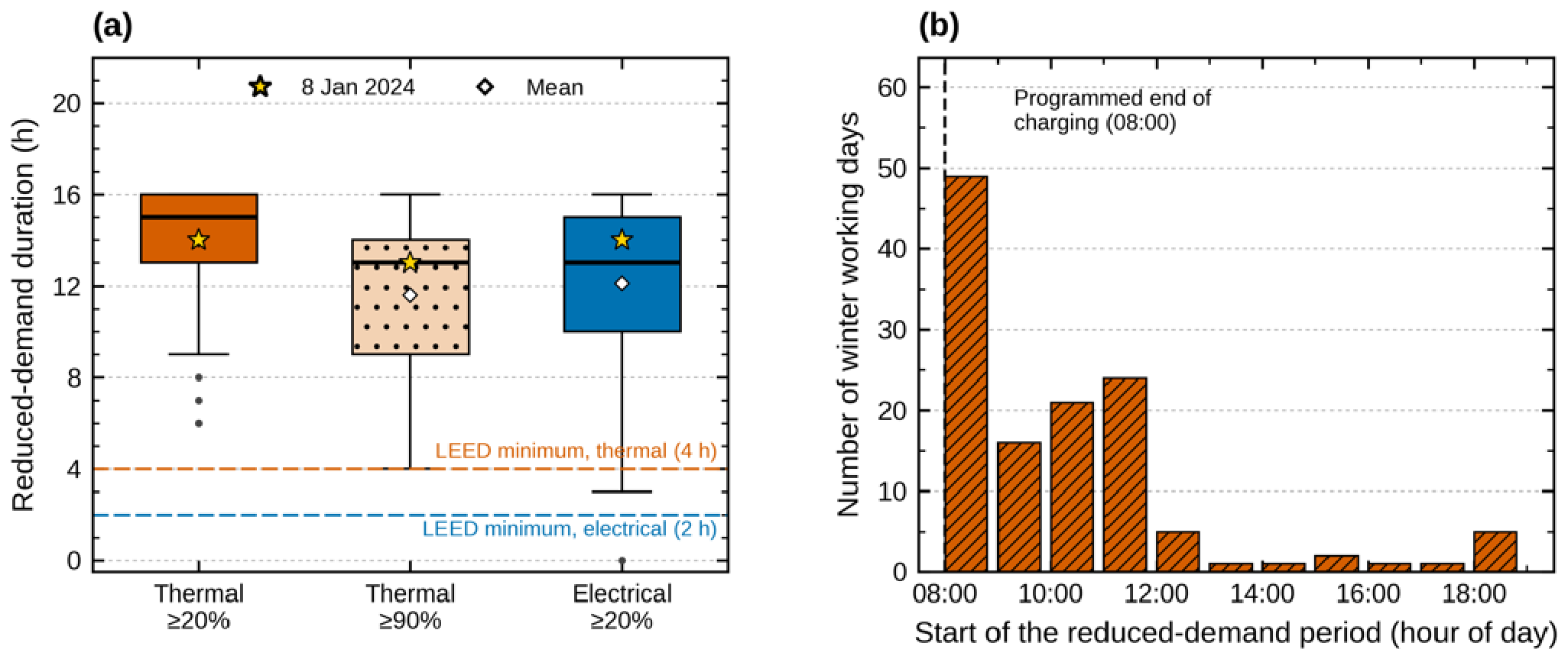
Table A1.
Statistics of the measured hourly demand on the winter working days of 2023 and 2024. Source: BMS of Apolonio Morales 29; created by the authors.
Appendix B. Full Simulation Period and Sensitivity Analysis
This appendix complements Section 3.2. Figure A2 shows the full 672 h simulated period for the six typologies, including the 120 h warm-up period excluded from the analysis, and Table A2 gives the complete results of the sensitivity analysis summarized in Table 7 (Section Sensitivity to the Infiltration Rate and the Supply Temperature). The underlying hourly data are provided in Excel Files S1–S3 (Supplementary Materials).
Table A2.
Sensitivity of the accumulated demand, the peak demand, the median recharge and discharge periods and the air- and surface-temperature differences between floors to the infiltration rate (at 30 °C) and to the supply temperature (at 0.2 ACH) for typologies 2 and 5. The reference case (0.2 ACH and 30 °C) is highlighted in bold to distinguish the baseline simulation from the sensitivity scenarios. Source: Excel Files S2 and S3; authors’ own simulations.
Figure A2.
Thermal demand, indoor air temperature, and slab surface temperature of the six simulated typologies over the full 672 h period (18 December–14 January), single-slab activation scenario. The hatched area marks the 120 h warm-up period excluded from the analysis, and the shaded bands mark the recharge and discharge phases. Source: Authors’ own simulations.
References
- Yang, X.; Li, Y.; Li, X.; Metwally, K.A.; Ding, Y. Activating and Enhancing the Energy Flexibility Provided by a Pipe-Embedded Building Envelope: A Review. Buildings 2025, 15, 2793. [Google Scholar] [CrossRef] [Scilit]
- Helsen, L. Geothermally activated building structures. In Advances in Ground-Source Heat Pump Systems; Rees, S.J., Ed.; Woodhead Publishing: Duxford, UK, 2016; pp. 423–452. [Google Scholar] [CrossRef] [Scilit]
- Kathirgamanathan, A.; De Rosa, M.; Mangina, E.; Finn, D.P. Data-driven predictive control for unlocking building energy flexibility: A review. Renew. Sustain. Energy Rev. 2021, 135, 110120. [Google Scholar] [CrossRef] [Scilit]
- Li, H.; Wang, Z.; Hong, T.; Piette, M.A. Energy flexibility of residential buildings: A systematic review of characterization and quantification methods and applications. Adv. Appl. Energy 2021, 3, 100054. [Google Scholar] [CrossRef] [Scilit]
- Cupeiro Figueroa, I.; Cigler, J.; Helsen, L. Model predictive control formulation: A review with focus on hybrid GEOTABS buildings. In Proceedings of the REHVA Annual Meeting Conference Low Carbon Technologies in HVAC, Brussels, Belgium, 23 April 2018. [Google Scholar]
- Gwerder, M.; Tödtli, J.; Lehmann, B.; Renggli, F.; Dorer, V. Control of thermally activated building systems. In Proceedings of the Clima 2007 WellBeing Indoors, Helsinki, Finland, 10–14 June 2007. [Google Scholar]
- Tödtli, J.; Gwerder, M.; Lehmann, B.; Renggli, F.; Dorer, V. TABS-Control: Steuerung und Regelung von Thermoaktiven Bauteilsystemen; Faktor Verlag: Zurich, Switzerland, 2009. [Google Scholar]
- Lehmann, B.; Dorer, V.; Gwerder, M.; Renggli, F.; Tödtli, J. Thermally activated building systems (TABS): Energy efficiency as a function of control strategy, hydronic circuit topology and (cold) generation system. Appl. Energy 2011, 88, 180–191. [Google Scholar] [CrossRef] [Scilit]
- Kalz, D.E. Heating and Cooling Concepts Employing Environmental Energy and Thermo-Active Building Systems for Low-Energy Buildings: System Analysis and Optimization. Ph.D. Thesis, University of Karlsruhe, Karlsruhe, Germany, 2009. [Google Scholar]
- Romaní, J.; de Gracia, A.; Cabeza, L.F. Simulation and control of thermally activated building systems (TABS). Energy Build. 2016, 127, 22–42. [Google Scholar] [CrossRef] [Scilit]
- Olsthoorn, D.; Haghighat, F.; Moreau, A.; Lacroix, G. Abilities and limitations of thermal mass activation for thermal comfort, peak shifting and shaving: A review. Build. Environ. 2017, 118, 113–127. [Google Scholar] [CrossRef] [Scilit]
- Lizana, J.; Chacartegui, R.; Barrios-Padura, A.; Ortiz, C. Advanced low-carbon energy measures based on thermal energy storage in buildings: A review. Renew. Sustain. Energy Rev. 2018, 82, 3705–3749. [Google Scholar] [CrossRef] [Scilit]
- Arteconi, A.; Costola, D.; Hoes, P.; Hensen, J.L.M. Analysis of control strategies for thermally activated building systems under demand side management mechanisms. Energy Build. 2014, 80, 384–393. [Google Scholar] [CrossRef] [Scilit]
- Lim, J.H.; Song, J.H.; Song, S.Y. Development of operational guidelines for thermally activated building system according to heating and cooling load characteristics. Appl. Energy 2014, 126, 123–135. [Google Scholar] [CrossRef] [Scilit]
- Yang, X.; Liu, D.; Tian, Z.; Deng, N.; Wang, R.; Jiang, Y.; Tang, R.; Zong, Y. Comparison of different control methods on the thermally activated building system (TABS) with large energy flexibility. Appl. Therm. Eng. 2024, 254, 123863. [Google Scholar] [CrossRef] [Scilit]
- Liu, D.; Yang, X.; Guan, W.; Tian, Z.; Zong, Y.; Tang, R. Model predictive control for heat flexibility activation of the Thermally Activated Building System. In Proceedings of the 18th IBPSA Conference on Building Simulation, Shanghai, China, 4–6 September 2023. [Google Scholar] [CrossRef] [Scilit]
- Hepf, C.; Overhoff, L.; Koth, S.C.; Gabriel, M.; Briels, D.; Auer, T. Impact of a weather predictive control strategy for inert building technology on thermal comfort and energy demand. Buildings 2023, 13, 996. [Google Scholar] [CrossRef] [Scilit]
- Silvestri, A.; Coraci, D.; Brandi, S.; Capozzoli, A.; Borkowski, E.; Köhler, J.; Wu, D.; Zeilinger, M.N.; Schlueter, A. Real building implementation of a deep reinforcement learning controller to enhance energy efficiency and indoor temperature control. Appl. Energy 2024, 368, 123447. [Google Scholar] [CrossRef] [Scilit]
- Sharifi, M.; Mahmoud, R.; Himpe, E.; Laverge, J. A heuristic algorithm for optimal load splitting in hybrid thermally activated building systems. J. Build. Eng. 2022, 50, 104160. [Google Scholar] [CrossRef] [Scilit]
- Michalak, P. Heat transfer by transmission in a zone with a thermally activated building system: An extension of the ISO 11855 hourly calculation method. Measurement and simulation. Energies 2025, 18, 2350. [Google Scholar] [CrossRef] [Scilit]
- Villar-Ramos, M.M.; Hernández-Pérez, I.; Aguilar-Castro, K.M.; Zavala-Guillén, I.; Macias-Melo, E.V.; Hernández-López, I.; Serrano-Arellano, J. A review of thermally activated building systems (TABS) as an alternative for improving the indoor environment of buildings. Energies 2022, 15, 6179. [Google Scholar] [CrossRef] [Scilit]
- De Saulles, T. Utilisation of Thermal Mass in Non-Residential Buildings; CCIP-020; MPA The Concrete Centre: Camberley, UK, 2007. [Google Scholar]
- Xu, X.; Yu, J.; Wang, S.; Wang, J. Research and application of active hollow core slabs in building systems for utilizing low energy sources. Appl. Energy 2014, 116, 424–435. [Google Scholar] [CrossRef] [Scilit]
- De Pereda Fernández, L. Integración de sistemas termoactivos para eficiencia. Principios y casos. In Guía sobre Estructuras Termoactivas y Sistemas Inerciales en la Climatización de Edificios; Fundación de la Energía de la Comunidad de Madrid (FENERCOM): Madrid, Spain, 2014; pp. 107–145. [Google Scholar]
- De Pereda Fernández, L. Modelo de actuación para la mejora de la eficiencia energética en la rehabilitación integral de un palacete protegido para oficinas de la Administración en Madrid. Geoterm. Estruct. Termoactivas An. Edif. 2015, 1, 1–9. [Google Scholar] [CrossRef] [Scilit]
- Reilly, A.; Kinnane, O. The impact of thermal mass on building energy consumption. Appl. Energy 2017, 198, 108–121. [Google Scholar] [CrossRef] [Scilit]
- Laera, R.; Martínez Pérez, I.; de Pereda Fernández, L.; Tendero Caballero, R.; Iannone, F. Control strategies, monitoring and management for the efficient behavior of Thermally Activated Building Systems (TABS). Build. Manag. 2019, 3, 7–23. [Google Scholar] [CrossRef] [Scilit]
- Laera, R.; Martínez Pérez, I.; de Pereda Fernández, L.; Tendero Caballero, R.; Iannone, F. The role of Thermally Activated Building Systems (TABS) in building energy retrofitting: Energy diagnosis and management. In Proceedings of the 13th International Conference Modern Building Materials, Structures and Techniques, Vilnius, Lithuania, 16–17 May 2019; pp. 625–633. [Google Scholar] [CrossRef] [Scilit]
- Directive (EU) 2024/1275 of the European Parliament and of the Council of 24 April 2024 on the Energy Performance of Buildings (Recast). Off. J. Eur. Union 2024, L 2024/1275. Available online: http://data.europa.eu/eli/dir/2024/1275/oj (accessed on 17 October 2026).
- U.S. Green Building Council (USGBC). LEED v5 for Operations + Maintenance: Existing Buildings (Beta Version); USGBC: Washington, DC, USA, 2023; Available online: https://www.usgbc.org/sites/default/files/2023-09/LEED-v5-OM-Existing-Buildings-beta-version_1.pdf (accessed on 17 October 2026).
- U.S. Green Building Council (USGBC). Summary of Changes to LEED v5: Operations + Maintenance (O+M); USGBC: Washington, DC, USA, 2025; Available online: https://www.usgbc.org/sites/default/files/2025-04/LEED-OM-v4-v5-Summary-of-Changes.pdf (accessed on 17 October 2026).
- U.S. Green Building Council (USGBC). LEED v5 O+M Rating System, November 2025 Edition; USGBC: Washington, DC, USA, 2025; Available online: https://www.usgbc.org/sites/default/files/2025-10/LEED%20v5%20O+M%20Rating%20System_November%202025_clean.pdf (accessed on 17 October 2026).
- BuildingGreen. LEEDuser: LEED v5 NC, EAc6 Grid Interactive. Available online: https://leeduser.buildinggreen.com/credit/NC-v5/EAc6 (accessed on 17 October 2026).
- U.S. Green Building Council (USGBC). LEED Project Directory. Available online: https://www.usgbc.org/projects (accessed on 17 October 2026).
- Ugalde, R. El Pequeño Edificio de Oficinas Español que ha Ganado a los Rascacielos de Todo el Mundo, El Confidencial. 2025. Available online: https://www.elconfidencial.com/inmobiliario/oficinas/2025-09-17/apolonio-morales-29-oficinas-sostenibilidad_4210046/ (accessed on 17 October 2026).
- Savills Spain, Savills Certifica Apolonio Morales 29, Primer Edificio en España con LEED v5 Platino y Récord Mundial de Puntuación. 2025. Available online: https://www.savills.es/publicaciones/noticias/380929/savills-certifica-apolonio-morales-29--primer-edificio-en-españa-con-leed-v5-platino-y-record-mundial-de-puntuacion (accessed on 17 October 2026).
- Eneres, Apolonio Morales 29, Líder Mundial con Certificación LEED Platinum EB:O+M v5. 2025. Available online: https://eneres.es/apolonio-morales-29-obtiene-leed-v5/ (accessed on 17 October 2026).
- EN 15378-3:2017; Energy Performance of Buildings—Heating and DHW Systems in Buildings—Part 3: Measured Energy Performance, Module M3-10, M8-10. CEN: Brussels, Belgium, 2017.
- IEC 62053-21:2020; Electricity Metering Equipment—Particular Requirements—Part 21: Static Meters for AC Active Energy (Classes 0,5, 1 and 2). IEC: Geneva, Switzerland, 2020.
- EN 1434-1:2022; Thermal Energy Meters—Part 1: General Requirements. CEN: Brussels, Belgium, 2022.
- DesignBuilder Software Ltd. DesignBuilder, Version 7.3.1.003; DesignBuilder Software Ltd.: Stroud, UK; Available online: https://designbuilder.co.uk (accessed on 17 October 2026).
- U.S. Department of Energy. EnergyPlus, Version 9.4. Available online: https://energyplus.net (accessed on 17 October 2026).
- Ministerio de Fomento. Real Decreto 732/2019, de 20 de diciembre, por el que se modifica el Código Técnico de la Edificación, aprobado por el Real Decreto 314/2006, de 17 de marzo (includes the Documento Básico DB-HE Ahorro de Energía). Bol. Of. Estado 2019, 311, 27. [Google Scholar]
- Babiak, J.; Olesen, B.W.; Petráš, D. Low Temperature Heating and High Temperature Cooling: Embedded Water Based Surface Heating and Cooling Systems; Babiak, J., Ed.; REHVA Guidebook No. 7; REHVA: Brussels, Belgium, 2007. [Google Scholar]
- EN 16798-1:2019; Energy Performance of Buildings—Ventilation for Buildings—Part 1: Indoor Environmental Input Parameters for Design and Assessment of Energy Performance of Buildings Addressing Indoor Air Quality, Thermal Environment, Lighting and Acoustics—Module M1-6. CEN: Brussels, Belgium, 2019.
- Ministerio para la Transición Ecológica y el Reto Demográfico; Ministerio de Vivienda y Agenda Urbana. Condiciones Técnicas de los Procedimientos para la Evaluación de la Eficiencia Energética de los Edificios; Ministerio para la Transición Ecológica y el Reto Demográfico: Madrid, Spain, 2026.
- ASHRAE. International Weather for Energy Calculations (IWEC Weather Files); ASHRAE: Atlanta, GA, USA, 2001. [Google Scholar]
- Thevenard, D.J.; Brunger, A.P. The development of typical weather years for international locations: Part I, algorithms. ASHRAE Trans. 2002, 108, 376–383. [Google Scholar]
- Iannone, F.; Franco, N.; Parisi, C.; Laera, R. Building Automation for Passive Cooling of Office Buildings: A Case Study in Madrid. In Proceedings of the 11th International Conference of Ar.Tec. (Colloqui.AT.e 2024); Corrao, R., Campisi, T., Colajanni, S., Saeli, M., Vinci, C., Eds.; Lecture Notes in Civil Engineering; Springer: Cham, Switzerland, 2025; Volume 611, pp. 375–389. [Google Scholar] [CrossRef] [Scilit]
- Velasco Gómez, E.; Andrés Chicote, M.; Rey Martínez, F.J.; Tejero González, A. Thermal behaviour of an active slab: Experimental study for TABs applications. Energy Procedia 2017, 142, 3326–3331. [Google Scholar] [CrossRef] [Scilit]
- Ding, Y.; Lyu, Y.; Lu, S.; Wang, R. Load shifting potential assessment of building thermal storage performance for building design. Energy 2022, 243, 123036. [Google Scholar] [CrossRef] [Scilit]
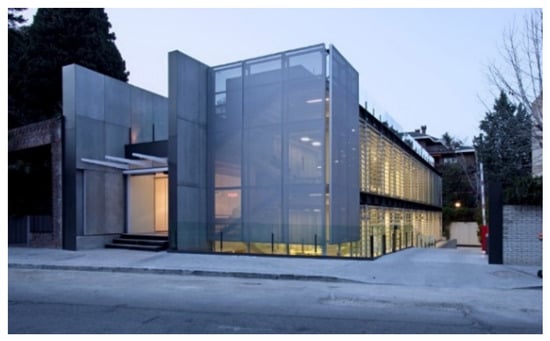
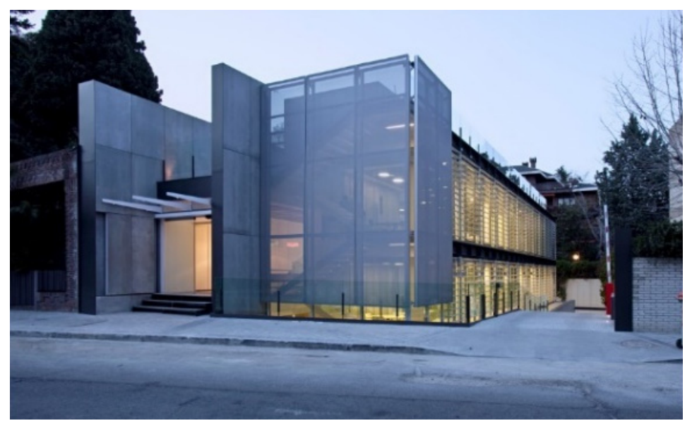
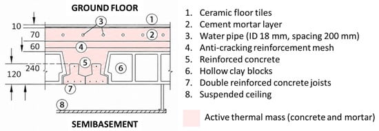
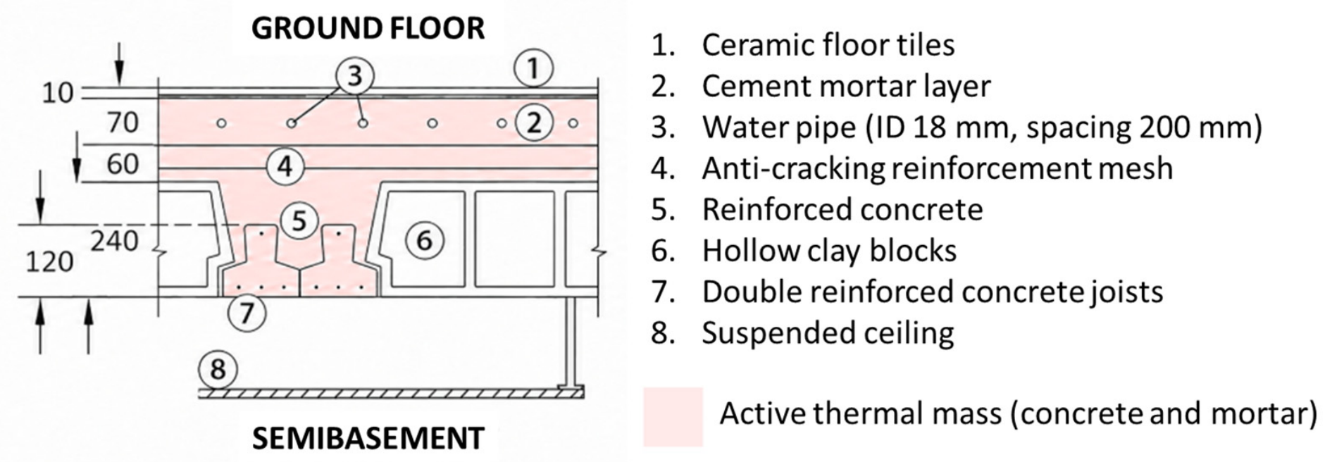
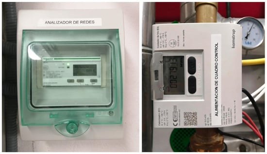
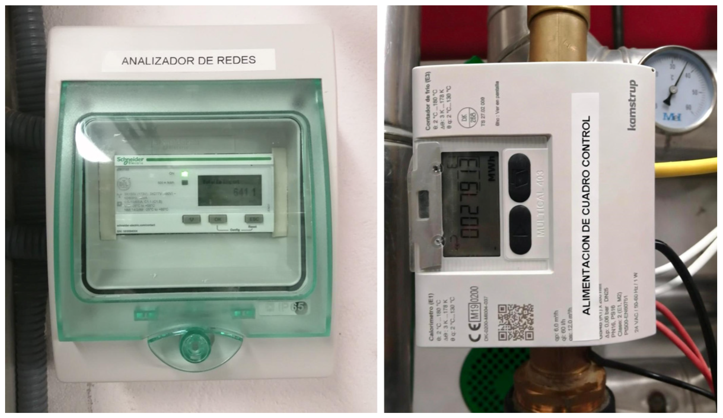
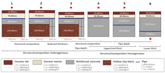
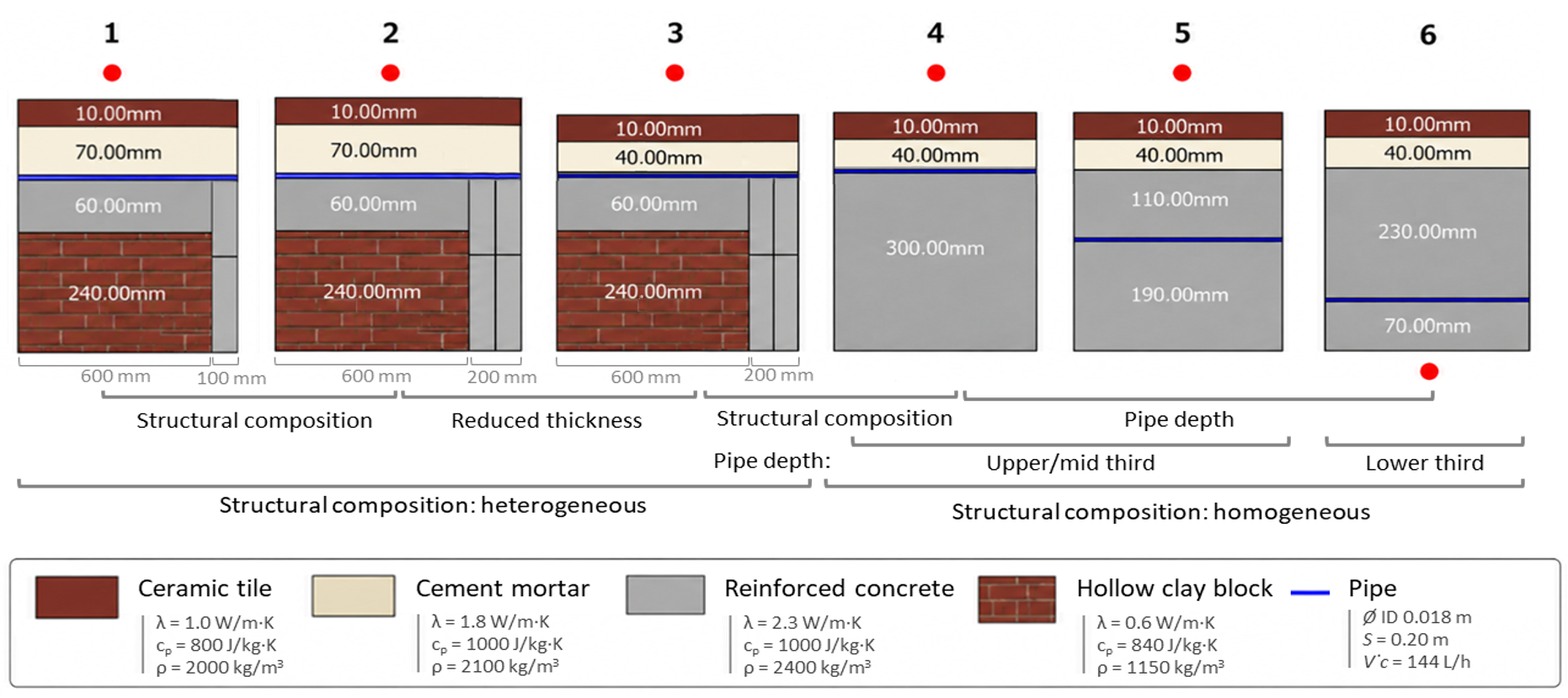
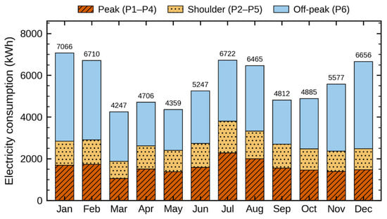
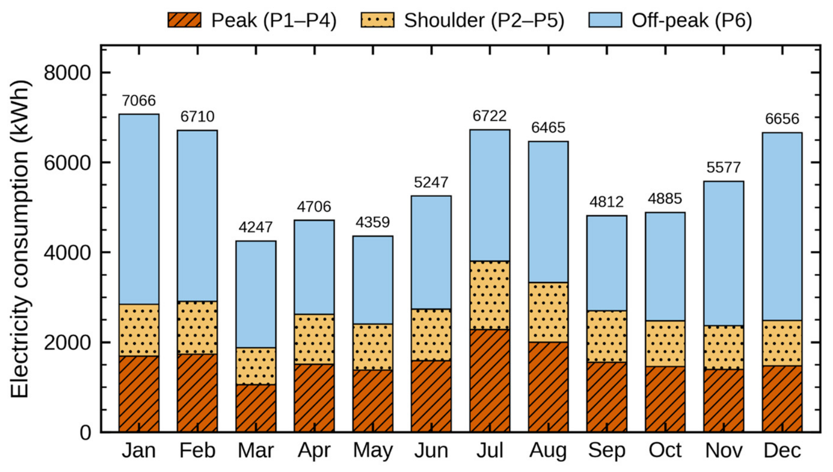
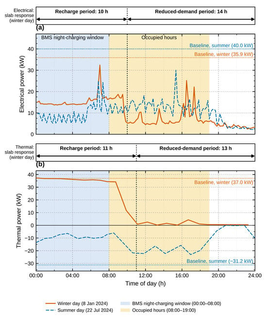
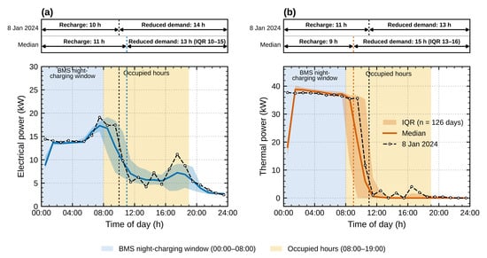
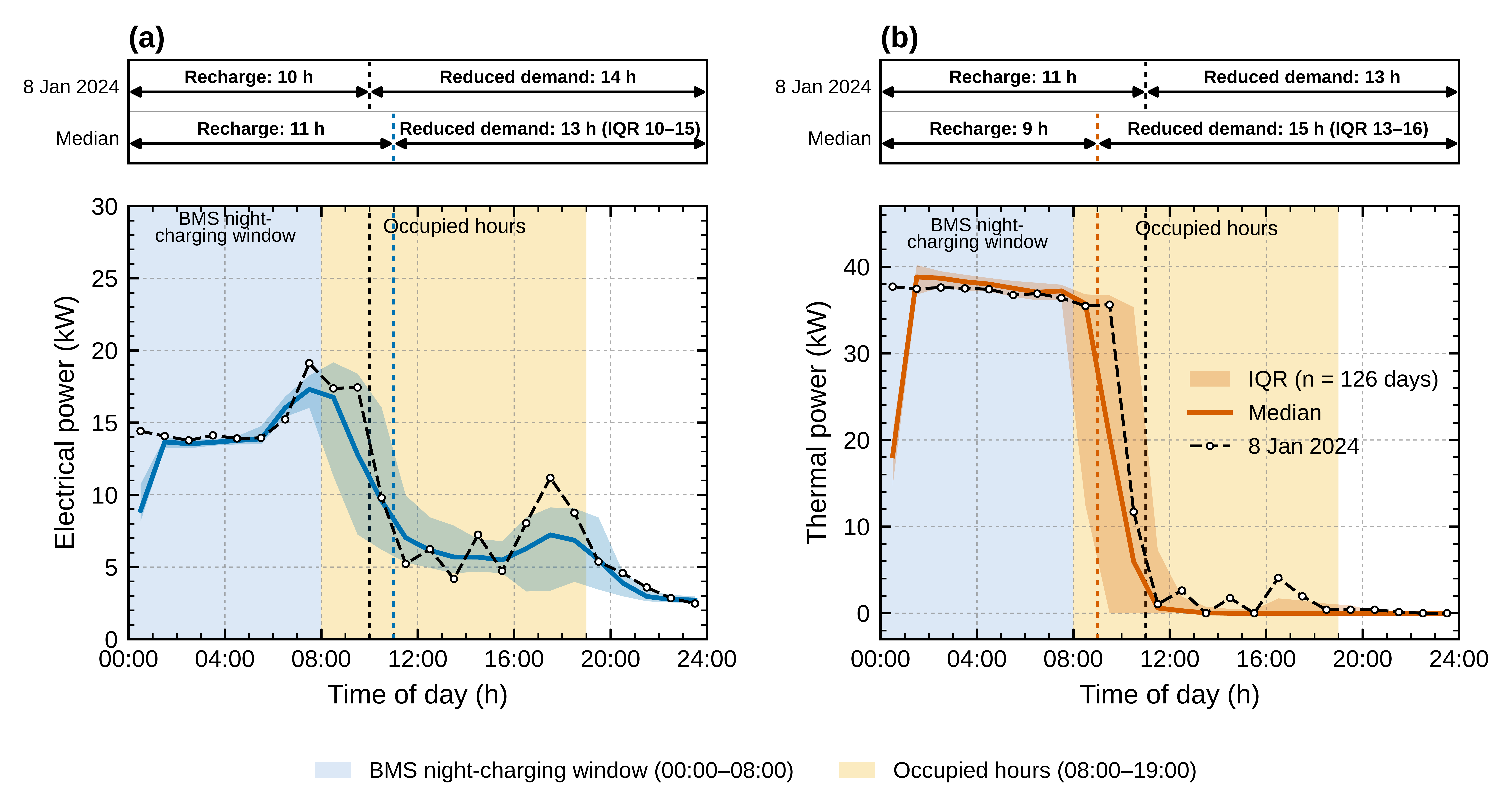
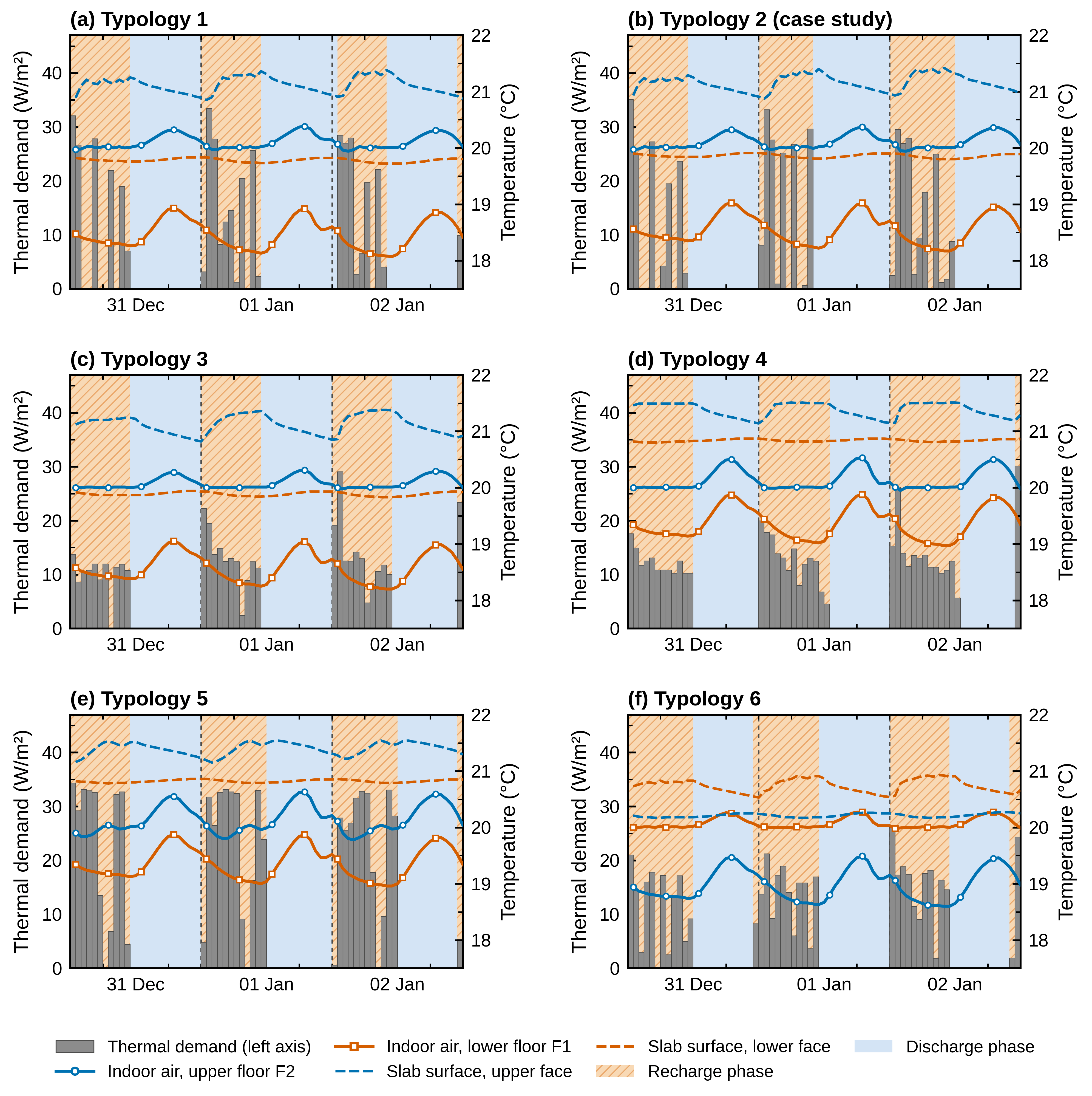

Disclaimer/Publisher’s Note: The statements, opinions and data contained in all publications are solely those of the individual author(s) and contributor(s) and not of MDPI and/or the editor(s). MDPI and/or the editor(s) disclaim responsibility for any injury to people or property resulting from any ideas, methods, instructions or products referred to in the content. |
© 2026 by the authors. Licensee MDPI, Basel, Switzerland. This article is an open access article distributed under the terms and conditions of the Creative Commons Attribution (CC BY) license.