


Abstract
The digital reuse of traditional woodcarving motifs requires coordinated consideration of category recognition, source relationships, and downstream geometric representation. This study develops and evaluates a modular workflow comprising semantic–structural recognition, manufacturing knowledge representation, and single-case toolpath construction to support motif documentation and machining preparation. Classification experiments used 1373 samples across 55 categories, with fixed three-fold partitions constrained by 1302 known-source proxy groups. Four model configurations were evaluated using three random seeds, yielding 36 runs. The manufacturing component separately documented relationships among five entity types and actual CAM configuration lookups. A single Baoxiang motif case was examined through archived NC toolpath reconstruction, idealized feed-motion time estimation, and two-dimensional tool-diameter sensitivity analysis. The semantic-only, full, concatenation, and structural-only configurations achieved mean macro-F1 scores of 44.21%, 43.91%, 43.20%, and 2.74%, respectively, indicating no consistent improvement from the current fusion configuration. Mean sample-level within-class similarity exceeded between-class similarity in all three test folds. The idealized feed-motion time subtotal for the Baoxiang case was 97.08 min. Under the specified scale and foreground-as-removal assumption, the geometrically unreachable foreground area fractions were 0.396% and 19.959% for assumed tool diameters of 1.5 and 4.0 mm, respectively. This study provides comparative recognition evidence under known-source grouping and a single-case geometric analysis workflow that may support architectural ornament cataloguing, candidate retrieval, and machining preparation. These findings do not establish complete physical-object independence, the incremental benefits of manufacturing recommendations, or physical machining accuracy.
1. Introduction
Traditional woodcarving motifs embody cultural memory, craftsmanship knowledge, and regional aesthetics. Their forms integrate symbolic meanings, decorative conventions, and accumulated manufacturing experience transmitted across generations. Recent advances in computer vision, three-dimensional digitization, and cultural heritage informatics have significantly improved the documentation, preservation, and retrieval of traditional artifacts [1,2,3,4]. Large-scale image acquisition and semantic annotation technologies have enabled computational analysis of cultural motifs, providing new opportunities for digital heritage conservation and design innovation [5,6].
However, digital preservation alone does not guarantee physical reproduction. Transforming a digitized motif into a wooden artifact still relies heavily on manual contour reconstruction, CAD refinement, and experience-based CAM parameter adjustment [7,8,9,10]. Unlike ordinary geometric objects, traditional woodcarving motifs contain culturally meaningful structures, variable-width strokes, organic curves, and fine decorative details. Their reproduction requires not only accurate visual understanding but also the preservation of geometric characteristics, carving logic, and manufacturing constraints [11]. Therefore, an effective computational framework should establish a continuous connection between motif perception, process knowledge, and CNC execution.
The transformation from motif images to CNC toolpaths involves several interconnected challenges. First, woodcarving images are often affected by wood grain, uneven illumination, aging, surface damage, shadows, and background interference, which complicate reliable motif extraction [5,12,13]. Second, traditional motifs exhibit strong intra-class similarity and subtle inter-class differences. Their recognition is further challenged by long-tailed category distributions, where frequent categories dominate model optimization and rare motifs remain difficult to identify [14,15,16,17,18,19]. Although vision-language models such as CLIP provide transferable semantic representations [20,21,22,23], their global features may overlook local structural characteristics, including stroke intersections, curvature variations, and boundary details that distinguish visually similar motifs. Third, converting raster-derived motif boundaries into CNC trajectories remains challenging. Direct vectorization usually produces dense and irregular control points, increasing interpolation burden and reducing machining efficiency [24,25,26,27]. For variable-width motifs, inappropriate tool-radius compensation may generate self-intersections, over-cutting, or disconnected regions when local geometric constraints conflict with tool dimensions [28,29]. Furthermore, machining parameter selection, including tool type, strategy, and cutting conditions, is still largely dependent on expert experience because the relationship between cultural motif semantics, geometric attributes, and manufacturing knowledge has not been systematically represented [30,31,32].
Existing studies have addressed individual aspects of this problem. Deep learning methods have achieved considerable progress in cultural heritage classification, retrieval, and digital reconstruction [3,4,33]. YOLO-based segmentation methods have demonstrated effectiveness in object extraction under complex visual conditions [12,13,34]. Fine-grained recognition approaches have introduced discriminative representation learning, focal-based optimization, and long-tail learning strategies to improve category-level recognition performance [14,15,35]. Vision-language pre-training and parameter-efficient adaptation methods further enhance domain transferability [20,21,36,37,38]. However, these approaches mainly focus on visual understanding and rarely establish a direct connection between recognized cultural patterns and executable manufacturing processes.
Knowledge graphs provide a potential solution for organizing heterogeneous knowledge involving products, processes, tools, materials, and manufacturing constraints [16,31,39,40]. In manufacturing applications, knowledge graphs have been explored for knowledge reuse, process recommendation, and decision support [7,9,32,41]. Nevertheless, existing approaches rarely consider cultural motif semantics and geometric characteristics as manufacturing knowledge sources. For traditional woodcarving, the relationships among motif categories, morphological attributes, tool selection, machining strategies, and process parameters remain insufficiently formalized.
Meanwhile, existing tool-radius compensation and trajectory optimization methods mainly target mechanical contours and industrial free-form surfaces [28,29,42]. Although smoothing techniques such as arc fitting, B-spline interpolation, NURBS reconstruction, and Chaikin corner cutting can improve trajectory continuity [25,26,27,42], they are not specifically designed for raster-derived cultural motifs containing narrow connections, variable widths, and organic decorative structures. A manufacturing-oriented strategy that integrates cultural semantics, geometric constraints, and CNC execution remains lacking.
In traditional architecture, woodcarving ornamentation simultaneously serves the functions of visual expression, cultural narrative, and component decoration, and its significance is related to its architectural location and context of use. Cao and Mustafa’s study of door and window carvings in Huizhou-style architecture shows that carving techniques and their application positions have regional characteristics; Zhao et al.’s study of window lattices in Zhaoyu Ancient City further reveals that motif composition is associated with architectural location and spatial function. Therefore, the digitization of architectural patterns requires not only identifying morphological categories in images but also preserving the connections between patterns and component positions, regional contexts, and contexts of use [43,44,45,46].
The corpus of this study consists mainly of images of furniture carvings and decorative panels. Among them, categories such as Bubujin (step-by-step brocade), ice-crack, ruyi, bat, pomegranate, and plum blossom correspond to some of the decorative motifs recorded in existing studies of architectural window lattices. This overlap at the motif level provides an entry point for cross-carrier retrieval and category organization, but it does not imply that different carriers share the same construction methods or manufacturing requirements. In particular, window lattices composed of wooden strips and connecting joints cannot be directly equated with the planar contour milling discussed in this paper.
On the basis of the above connections, this study limits its research object to pattern image recognition, visual relationship representation, and single-case toolpath construction. It focuses on recognition performance under a fixed corpus and split conditions, as well as the implementation process of converting image geometry into program paths. Architectural relevance is reflected in the organization of decorative motifs and front-end information preparation for machining, rather than in validating the entire process of restoring architectural components.
Therefore, three research gaps remain. First, existing cultural heritage digitization approaches lack an integrated pathway that transforms motif images into CNC-executable manufacturing instructions. Second, current knowledge-graph-based manufacturing approaches rarely establish explicit links between learned cultural representations, motif geometry, and machining decisions. Third, existing trajectory-generation methods are insufficiently adapted to the geometric characteristics of traditional motifs, particularly variable-width structures and narrow morphological connections.
To address these gaps, this study develops a semantic-to-toolpath framework for CNC reproduction of traditional woodcarving motifs. The main contributions are summarized as follows:
- (1)
- A documented evaluation protocol for a 55-category, 1373-image woodcarving corpus. Frozen three-fold partitions use 1302 known-source proxy groups to keep identified related records within the same partition. Out-of-fold predictions provide a common basis for comparison across three random seeds. This protocol addresses identified source relationships without assuming complete physical-object independence.
- (2)
- An implementation and comparative evaluation of semantic–structural residual fusion. We compare the full model with semantic-only, structural-only, and concatenation configurations. Across 36 runs, the comparison establishes the empirical contribution and limitations of the implemented configurations: the pre-trained semantic configuration serves as a strong reference, while adding the current structural branch does not consistently improve Macro-F1. Sample-level and category-center similarity analyses further characterize the learned test representations.
- (3)
- An explicit separation of visual similarity, heterogeneous manufacturing relations, and executable category-to-configuration lookup. A five-entity-type representation and its relation paths are documented alongside the actual CAM configuration outputs, making their correspondence and differences inspectable. This component provides a traceable representation of the workflow interfaces rather than evidence of automated manufacturing inference.
- (4)
- A computational characterization of a single Baoxiang toolpath case. This combines archived NC path reconstruction, a decomposition of idealized feed-motion time, and a controlled two-dimensional tool-diameter accessibility analysis. These analyses describe program behavior and geometric sensitivity under stated assumptions. An existing specimen photograph supplies a separate qualitative illustration.
2. Materials and Methods
2.1. Research Framework and Evaluation Scope
This study comprises four components: offline image preparation, semantic–structural recognition, manufacturing knowledge representation, and single-case CAM toolpath construction. The workflow, illustrated in Figure 1, is organized into two parts: recognition with grouped evaluation, and manufacturing representation with single-case evidence. The recognition component uses frozen image inputs and fixed data partitions, with classification performance assessed using out-of-fold (OOF) predictions. The manufacturing component separately documents an explicit relation graph, manually supplied CAM inputs, geometric toolpath construction, archived NC reconstruction, and a physical Baoxiang carving demonstration. The results of these two components are reported and interpreted separately.
Figure 1.
Research workflow.
The classification experiments use images specified in the frozen manifest and evaluate recognition performance on group-constrained test partitions. The manufacturing relation example and CAM configuration lookup are reported independently; the selected image and motif category are manually supplied to the CAM entry point. Archived NC reconstruction and specimen photographs are presented separately. Data-flow connections in the workflow diagram represent implemented operations, while conceptual associations are not depicted as verified automated inference connections. Classification experiments involve 1373 samples, three fixed folds, and three random seeds. The manufacturing component comprises a limited relation graph, a comparison against the default configuration, and the Baoxiang case. Throughout this study, the term “semantic branch” refers to the CLIP-pretrained visual representation branch; it does not imply the use of textual motif descriptions or cultural-semantic inference.
The physical machining demonstration was performed using a Sandu 8080 three-axis CNC engraving machine (Jinan Sandu CNC Equipment Co., Ltd., Jinan, China), with the wooden workpiece secured using standard mechanical clamps. The specimen photograph provides qualitative evidence of the machining demonstration and is reported separately from the computational analyses.
2.2. Dataset Construction and Quality Control
2.2.1. Data Sources and Corpus Composition
The initial collection comprised 1887 image records of woodcarving and traditional decorative motifs, assembled from four source types: enterprise photographs (n = 1150), cultural heritage archives (n = 350), books (n = 240), and digital pattern resources (n = 147). These sources included photographs of carved objects from three Chinese traditional solid-wood furniture manufacturers, archival images from cultural heritage institutions, scanned illustrations and plates from books, and digital motif and pattern materials. The corpus therefore included object photographs, line drawings, and digital pattern materials. The initial collection count describes the scale of corpus preparation; the formal classification experiments are defined by the frozen sample manifest.
Following initial collection, deduplication, cleaning, and auditing, 1373 samples were retained for classification: enterprise photographs (n = 800), cultural heritage archives (n = 250), books (n = 200), and digital pattern resources (n = 123). The difference between the initial and final counts was 514 records. Of these, 497 were accounted for by the three reported exclusion categories: 376 duplicate records, 67 records with insufficiently recognizable motifs, and 54 records lacking annotations. The remaining 17 records were associated with historical inclusion-status entries, comprising nine previously marked “exclude” and eight previously marked “keep.” All 17 were finally removed after adjudication; the historical status labels do not, by themselves, establish the final disposition of individual records. The eight records historically marked “keep” reflected an intermediate curation state rather than a final retention decision and were reclassified as removed following duplicate/homologous-image grouping, legacy-image replacement, or proxy-group construction. The final disposition, documented reason, related retained sample ID, and audit reference for each of these 17 records are provided in Supplementary Table S13a. Accordingly, the full difference reconciles as 1887 initial records − 1373 retained records = 514 removed records = 497 exclusion-category records + 17 individually documented records. All experimental counts are based on the final sample-ID manifest.
The final corpus comprises 55 categories. Category counts, fold-specific allocations, and totals are provided in Supplementary Table S3. Three-fold cross-validation was used, with each sample appearing in the test set exactly once across the three outer folds. The training/validation/test counts were 702/213/458, 703/213/457, and 702/213/458 for Folds 1, 2, and 3, respectively, with 1373 samples represented in each fold. Across the three folds, these allocations correspond to 2107 training assignments, 639 validation assignments, and 1373 test assignments, rather than additional unique samples. The approximate within-fold proportions were 51.1%, 15.5%, and 33.4%, respectively.
Category sizes ranged from 4 to 92 samples, with a mean of 24.96, a median of 20, and a maximum-to-minimum ratio of 23. Six categories contained fewer than 10 samples—orchid, cross-cloud, lingzhi, pomegranate, gourd, and interlocking-ring motifs—accounting for 48 samples, or 3.5% of the corpus. Five categories contained at least 50 samples—bogu (antiquities), fret, longevity-character, scrolling-foliage, and dragon motifs—accounting for 345 samples, or 25.1%. The remaining 44 categories contained 10–49 samples each. Category labels were assigned according to the visually dominant form and established motif terminology and remained frozen throughout the experiments.
Classification labels and segmentation instances were recorded separately. Each classification sample was assigned one category label, whereas the annotation protocol required spatially distinct motif instances within an image to be annotated individually. For composite motifs, the visually dominant motif determined the primary category, while secondary motifs were recorded in the notes. Cases without a clearly identifiable dominant category entered the dispute-resolution process. The presence of a motif category in an image does not imply that all decorative regions were annotated as that category or that every instance was included in the classification dataset.
Source-stratified initial and retained counts, together with source descriptions, are reported in Supplementary Table S13; the 17 individually documented records are listed in Supplementary Table S13a. The 1373 retained images refer to the final retained set across all four source types, not to enterprise photographs alone. Source-level licensing, permission, and disclosure restrictions are retained in internal documentation and are available for editorial verification; they are not publicly released because of confidentiality and copyright restrictions. Enterprise names, archive identifiers, and authorization-document identifiers were de-identified. Original enterprise images are not publicly released because of confidentiality and copyright restrictions. De-identified thumbnails, record-level statistics, and model predictions are available upon request; authorization documentation and original file paths are provided exclusively for editorial verification.
2.2.2. Annotation Rules and Four-Stage Quality Control
- (1)
- Annotation tasks and category definitions
The annotation tasks comprised delineating polygon masks along the visible boundaries of target motifs and assigning labels from 55 predefined categories. The trained first author served as the initial annotator (A) and performed the annotations according to standardized guidelines. Category assignment was based on the dominant motif structure and its associated meaning. For composite motifs, the visually dominant motif was assigned as the primary category, while secondary motifs were recorded in the notes. Cases in which the dominant category could not be determined were referred for expert arbitration.
- (2)
- Four-stage review and personnel responsibilities
Quality control followed four stages: initial annotation, expert review, disagreement arbitration, and final verification. Expert E2 directly inspected the initial annotations, reviewing boundary delineation, composite-motif categorization, and the treatment of damaged regions. Disagreements were referred to E3 for arbitration, after which E1 verified the category taxonomy and final decisions. E2’s review constituted non-blinded annotation quality control and was limited to cross-checking dataset annotations; it did not constitute an independent evaluation of downstream manufacturing recommendations. Expert backgrounds and responsibilities are presented in Table 1.
Table 1.
Backgrounds and actual responsibilities of annotators.
- (3)
- Geometric boundaries and mask specifications
Polygons followed the visible motif boundaries without inferring or reconstructing damaged, occluded, or missing portions. Ambiguous boundaries were delineated conservatively and referred for review. Spatially distinct motif instances within the same image were annotated separately. For structural holes, internal boundaries were recorded and preserved during mask export to prevent these regions from being incorrectly filled as foreground. Bounding-box and point annotations were not accepted as valid polygon masks for segmentation training.
- (4)
- Quality-control records and evaluation scope
The classification manifest and valid segmentation-mask inventory were maintained separately. Consequently, the 1373 classification samples do not define the segmentation training or test-set size. Classification evaluation was conducted strictly using the actual input images specified in the frozen classification manifest.
Annotation review records were linked by sample ID and included the initial annotation, review comments, disagreement type, arbitration decision, final verification, and inclusion status. Missing historical entries were designated as “not recorded,” and supplementary reviews were documented using their actual dates of completion. Although the four-stage protocol specifies review responsibilities, the early archives did not retain complete sample-level review statuses or paired labels recorded before adjudication. Accordingly, no full-dataset review coverage rate or inter-rater agreement coefficient, such as Cohen’s kappa, is reported. Agreement in the final labels is not treated as a substitute for pre-adjudication agreement. Explicit arbitration decisions were retained for all disputed samples, and the recording requirements for each stage are detailed in Supplementary Table S2.
2.2.3. Known-Source Grouping and Three-Fold Partitioning
Formal samples are associated with categories, relative paths, current file hashes, historical original file hashes, and effective group identifiers via sample IDs. Based on identified duplicates, homologous, and derived associations, a total of 1302 proxy groups were established, comprising 1242 single-sample groups and 60 multi-sample groups. The partitioning is constrained by the effective group, assigning an entire group to a single subset. Proxy groups describe known source relationships and are not equivalent to physical collection numbers.
In each fold, the training, validation, and test sets are mutually exclusive, and the same effective proxy group cannot span across these partitions. Let the three subsets of the f-th fold be , , and , and the group mapping be , then the following constraints are satisfied:
where .
The frozen classification dataset comprises 1373 unique samples from 55 classes, organized into the 1302 known-source proxy groups. Supplementary Table S12 provides the anonymized sample ID, class label, proxy-group ID, and training, validation, or test assignment of every sample in each of the three folds. The training/validation/test counts are 702/213/458, 703/213/457, and 702/213/458, respectively (Table 2). Each sample has exactly one subset assignment within each fold and appears in the test subset in exactly one of the three folds. To evaluate the model’s sensitivity to initialization and optimization processes, three random seeds (42, 43, 44) use the exact same frozen partition. This means the random seeds only alter the initialization of network weights and the randomness during training (e.g., dropout and data shuffling), rather than regenerating the data partitions.
Table 2.
Sample sizes of the three folds for the formal classification experiment.
Direct checks of the sample-level manifest identified zero pairwise intersections between the training, validation, and test subsets within each fold for sample IDs and proxy-group IDs. The corresponding intersections were also zero for the recorded current MD5, SHA256, pixel SHA256, and original MD5 identifiers. These hash checks concern the identifiers recorded in the frozen manifest. The split-file hash recorded in all 36 formal runs matches the recovered frozen split file, and the test prediction rosters and class labels agree with the corresponding test assignments.
These checks establish consistency of the recorded partitions and separation of identified source relationships. They do not establish complete physical-object independence. Where correspondence to an original physical object cannot be verified, different photographs or scans of the same object may remain unrecognized as related records. This limitation is retained when interpreting the classification results. Furthermore, the reuse of samples across different outer folds is a standard cross-validation arrangement. Class imbalance is described using per-class sample sizes and macro-average metrics, and results for the many-shot group (N ≥ 50) that are empty in the current training fold are not adopted. Sample-level subset assignments and proxy-group identifiers are provided in Supplementary Table S12.
2.2.4. Motif Region Representation and Classification Preprocessing
The segmentation module is used to generate candidate motif regions. For an input image I and a binary mask M, the foreground representation with the background set to zero is expressed as:
where u and v are pixel coordinates, and k is the color channel; the bounding region of the foreground area Ω is cropped to obtain the candidate instance image. This operation defines the mask-assisted foreground representation.
The formal classification program directly reads the offline images from the frozen list and does not call the segmentation model online during classification training; therefore, the classification experiment evaluates the recognition performance under fixed input conditions. YOLOv8m-Seg is only used for preliminary motif candidate region extraction, and its archived configuration is provided in Supplementary Table S5. This module is introduced as a preprocessing tool in this study and is not included in the independent performance evaluation; it should be specifically noted that the 1373 samples of the classification set and the three-fold partition are not used as the scale of the segmentation data. This paper does not infer segmentation generalization performance based on classification results, nor does it report mIoU or pixel accuracy lacking corresponding independent test evidence.
Classification inputs are uniformly converted to RGB and resized to 224 × 224. During the training phase, the following augmentations are sequentially applied: horizontal flipping with a probability of 0.5, random rotation of ±15°, random translation of up to 5% in both horizontal and vertical directions along with 0.9–1.1 times scaling, brightness/contrast/saturation perturbation with an amplitude of 0.2, and grayscale conversion with a probability of 0.05. The validation and testing phases only perform resizing, tensor conversion, and normalization. Training augmentations are generated online, are not counted as the 1373 independent samples, and are not distributed across subsets. The channel means for the dual-branch model are [0.48145466, 0.45782750, 0.40821073], and the standard deviations are [0.26862954, 0.26130258, 0.27577711].
2.3. Semantic–Structural Dual-Branch Motif Recognition
2.3.1. Global Visual Semantic Branch
To extract the global visual representation of motifs, the semantic branch is constructed using the ViT-B/32 vision encoder of the pre-trained CLIP model [20]. The input images are uniformly resized to 224 × 224 pixels and split into 7 × 7 non-overlapping 32 × 32 pixel patches. The vision encoder outputs a 768-dimensional pooled feature, which is then mapped to a 512-dimensional embedding space via a pre-trained visual projection layer. The term “semantic branch” in this paper refers to the image encoding branch utilizing CLIP’s pre-trained visual representations; the text encoder does not participate in the classification computation of this study.
To unify the feature scale, an L2 normalization function is defined as:
where is a numerical stability constant set to avoid division by zero.
For an input image x, the global visual semantic feature is expressed as:
where denotes the vision encoder, is the pre-trained visual projection matrix, and is the normalized output of the semantic branch.
During training, only the last two Transformer blocks of the visual encoder and the visual projection layer are fine-tuned, while the remaining CLIP parameters remain frozen. This setting exploits pretrained visual representations while adapting to the woodcarving pattern classification task through partial parameter updates. The output of the semantic branch and the output of the convolutional structural branch are jointly input into the residual fusion module, and the overall network structure is shown in Figure 2. The semantic branch was initialized from the OpenAI CLIP ViT-B/32 checkpoint distributed through the Hugging Face repository openai/clip-vit-base-patch32 and loaded using transformers.CLIPModel.from_pretrained. The archived configurations of all 27 formal runs using CLIP record the resolved repository revision 3d74acf9a28c67741b2f4f2ea7635f0aaf6f0268. This revision was recorded from the loaded model configuration; the historical loading call did not explicitly specify a revision argument. The nine structural-only runs did not load CLIP. Supplementary Table S4 reports the pretrained checkpoint identifier, loading interface, and recorded revision. These pretrained-model identifiers are distinct from the experiment-specific fine-tuned checkpoints selected using validation performance.
Figure 2.
Recognition architecture.
The structural branch is a three-layer convolutional network trained from scratch and does not contain ResNet residual blocks. Each layer sequentially applies a 3 × 3 convolution, Batch Normalization, and GELU; the convolution stride is 2 and the padding is 1, and the channel dimensions are 3 → 64 → 128 → 256. Let = x. Then
The spatial dimensions of the three feature maps are 112 × 112, 56 × 56, and 28 × 28, respectively. The final feature map is subjected to global average pooling, linear projection, layer normalization, and L2 normalization to obtain the structural vector:
The projection output dimension of the structural branch is 512. This branch learns local convolutional features through class supervision and forms an image-level structural representation via global pooling; the network structure consists of the above three convolutional layers and the projection.
2.3.2. Residual Fusion and Classification
The two 512-dimensional branch features are first concatenated and then passed through a linear mapping, layer normalization, GELU activation, and Dropout with a rate of 0.2 to obtain the fusion residual. This residual is scaled by a learnable scalar, added to the semantic feature, and subjected to L2 normalization:
where denotes vector concatenation, , and is used for numerical stability; N denotes L2 normalization; α is a trainable scalar without an imposed value-range constraint, initialized to 0.1. This design adopts ReZero-inspired residual scaling but uses non-zero initialization. The residual mapping simultaneously receives semantic and structural features, and the semantic branch also directly participates in the fusion through a skip connection.
The classification head consists of two linear layers. After the first layer, layer normalization, GELU, and Dropout with a rate of 0.5 are applied sequentially:
where , , is the logits output by the classification head, and p is the class probability computed from it; this does not require an additional Softmax layer to be added inside the classification head in the code. Dropout is enabled during training and disabled during evaluation; the final class is . Layer normalization is located inside the residual mapping and the classification head, and the final fused vector uses L2 normalization; the two normalizations are not interchangeable.
2.3.3. Class Weighting and Smoothed Focal Loss
Class weights are computed only from the training samples of the current fold. Let the number of classes be C = 55, the total number of training samples be , and the number of training samples in class . Then
For the idea of focal modulation, see Ref. [14]. The training set of each current fold covers all classes, so . For a batch of size B, the loss is
where is the total number of training samples in the current fold, is the number of training samples in class c, and B is the actual number of samples in the current mini-batch. Both the class weight and the focal modulation term are computed according to the true class and act on the entire smoothed cross-entropy term. Label smoothing makes the target probability of the true class , and that of the remaining classes /C. The training set of each fold covers all 55 classes. The number of training samples in fold 1 is 702, and the corresponding class weight range is 0.31909–6.38182. The class frequencies of the validation and test sets do not participate in weight computation.
2.3.4. Training Control and Ablation Definitions
Training uses AdamW. The learning rate is for the trainable CLIP parameters and for the structural branch, fusion layer, and classification head, with a weight decay of . The maximum number of training epochs is 80, and the learning rate is scheduled by cosine annealing without warm restarts:
The mini-batch size is 2, gradient accumulation is 8 steps, and the nominal effective batch size is 16. For an accumulation window W, the loss is weighted according to the actual number of samples in that window: . When the final window contains fewer than 16 images, it is still computed according to the actual number of samples. The global gradient norm clipping threshold is 1.0. Gradient accumulation does not change the mini-batch seen by Batch Normalization in each forward pass, so this setting cannot be interpreted as a BN batch size of 16.
In each epoch, the best weights are selected according to the validation macro-F1; early stopping is triggered when there is no strict improvement for 15 consecutive epochs. Test evaluation uses the weights corresponding to the best validation epoch, and the last epoch is not automatically used as a substitute. The three random seeds are 42, 43, and 44. Checkpoints save the model, optimizer, scheduler, random states, epoch, and best-model information; when the same experiment is resumed, the total number of epochs and the device type are kept unchanged.
The three folds of seed 42 and the first two folds of seed 43 for the full model were run on an NVIDIA T600, and the remaining four runs used CPU; internal ablations used CPU. The software environment is Python 3.9.25, PyTorch 2.6.0+cu118, torchvision 0.21.0+cu118, transformers 4.57.6, NumPy 2.0.2, scikit-learn 1.6.1, and Pillow 11.3.0. The device is recorded according to the run log; fixed seeds do not guarantee bitwise consistency across CPU and GPU.
The experimental settings include the full model (full) and three internal ablation variants: semantic branch only (semantic), structural branch only (structural), and concatenation mapping (concat). The single-branch variants feed the corresponding 512-dimensional normalized feature into the classification head; concat retains the dual-branch concatenation mapping and directly applies L2 normalization to the resulting residual vector before feeding it into the classification head, removing the semantic skip connection and its residual scaling fusion. The four configurations use the same frozen data splits, training control, and evaluation metrics, and each completes experiments with three random seeds and three folds, totaling 36 runs.
2.3.5. Evaluation Metrics and Inter-Seed Statistics
Let the numbers of true positives, false positives, and false negatives for class , , and , respectively. Define
Macro-precision and macro-recall are the class averages of and , respectively; zero denominators are treated as 0, and all 55 classes are included in the average. Accuracy is the proportion of correctly classified samples among all test samples.
For each seed, the predictions from the three non-overlapping test folds are concatenated into 1373 out-of-fold predictions, and then the metric for that seed is computed, rather than simply averaging the macro-F1 of the three folds first. The mean and sample standard deviation of the three seeds are
The mean and standard deviation are reported on a consistent metric scale; when a metric is expressed as a percentage, the standard deviation is expressed in percentage points. This standard deviation is used to describe the variability of repeated experiments under the fixed splits and actual runtime conditions, and is not used as a confidence interval for generalization performance. Because some full-model experiments used different computing devices, the observed variability is not entirely attributable to random seeds. This paper does not treat the nine-fold results as nine independent repeated experiments, nor does it claim a statistically significant advantage based on the descriptive differences among the three seeds.
2.4. Pattern Similarity Relationships and Manufacturing Knowledge Representation
2.4.1. Class Similarity Relationships and Feature Space Analysis
Class similarity relationships are used to describe the visual representations learned by the recognition model, whereas manufacturing knowledge representation is used to organize the heterogeneous relationships among patterns, attributes, cutting tools, machining strategies, and parameters. The two are conceptually linked through pattern class names but serve different tasks.
Feature analysis was performed separately for the three test folds of the full model under seed 42, using the features associated with each fold’s best-validation checkpoint. Features produced by independently trained fold models were not pooled into a common feature space.
For a given fold, let T denote the set of test-sample indices, the class label of sample i, and its feature vector. The normalized feature and sample-level cosine similarity are defined as
All supplied test features were finite and had nonzero norm. A non-finite or zero-norm feature would be ineligible for cosine-similarity analysis; no such exclusion was required in the present data.
For class c, let . The class center and class-center cosine similarity are
Center similarities are defined for nonzero class centers. Their diagonal entries equal one by construction and are not used to measure within-class consistency.
For each sample anchor i, define the eligible within-class and between-class comparison sets as
The corresponding eligible anchor sets are and . Sample-level within-class similarity is
Sample-level between-class similarity is
Both statistics are computed by averaging over eligible comparison samples within each anchor, and then equally averaging across eligible anchors. They are not unweighted averages over classes or equal-weight averages over all pooled sample pairs.
Self-comparisons are excluded from within-class similarity. Classes represented by only one test sample contribute no within-class anchor, but their samples remain eligible for between-class comparisons and class-center analysis. All test samples have between-class comparators in the present folds. No additional exclusion of within-proxy-group pairs was applied; these are sample-level descriptive statistics rather than estimates based on independently verified physical objects. A statistic is undefined if its eligible anchor set is empty.
The two-dimensional visualization of features uses t-SNE, computed separately for each fold. The parameters are set to perplexity 30, learning rate 200, early exaggeration 12, 1000 iterations, PCA initialization, and random seed 42. Class labels are used only for coloring the results. This analysis is intended to explore the representation distribution of test samples and is not used as independent evidence for the validity of manufacturing rules or model superiority. The specific results are shown in Table 3.
Table 3.
Sample-level intra-class and inter-class cosine similarities of each test fold of the full model under seed 42.
2.4.2. Entities and Relations of Manufacturing Knowledge
The manufacturing knowledge representation is defined as , where the entity set is divided into five categories: patterns , geometric or morphological attributes , cutting tools , machining strategies , and parameters ; the triples satisfy
Relations can represent that a pattern has a certain attribute, that a pattern is associated with a certain cutting tool or strategy, and that a cutting tool or strategy uses a certain parameter. Class names in the class similarity network can serve as concept correspondence keys, but their edge weights do not automatically constitute the confidence of manufacturing rules, nor can the 55-node similarity graph be regarded as a complete manufacturing graph containing the five entity types.
This example contains 2 pattern entities, 2 attribute entities, 2 cutting tool entities, 4 strategy entities, and 7 parameter entities, totaling 17 nodes and 16 directed relations. Supplementary Materials Tables S6–S8 list the complete node list, relation triples, and path retrieval examples.
The manufacturing knowledge representation is used to demonstrate the five entity types and their process associations, and its coverage is limited to the listed example. The manufacturing graph implemented in this paper does not form an automatic execution chain with downstream CAM configuration queries; CAM uses an independent category–configuration mapping. Therefore, the relations in the graph are used for knowledge organization and path retrieval, and are not used to report incremental performance of automatic tool selection or manufacturing recommendation. The class similarity network establishes conceptual correspondence with the manufacturing representation through pattern names, but visual similarity edges do not automatically generate process rules. The example tool associations in the manufacturing graph and the actual configurations adopted by CAM are reported separately; differences between the two are not interpreted as intermediate results and final decisions of the same reasoning process.
2.4.3. Category-Driven CAM Configuration Query
The downstream CAM program adopts an explicit mapping from categories to parameter configurations. If the input category c exists in the configuration dictionary K, the corresponding configuration is returned; otherwise, the default configuration is adopted:
The CAM program queries the configuration dictionary according to the input category and returns the default configuration when no corresponding entry exists. In the current implementation, both Baoxianghua and Wanzi patterns use the default configuration, including a nominal tool diameter of 1.5 mm, spindle command S24000, feed command F300–F1000, layer stepdown of 0.5 mm, and target depth of −2.0 mm. Whether to adopt the result after graph retrieval or adjust it based on experience is a manual process decision. This process establishes a deterministic interface between category input and machining configuration and does not involve attribute constraint solving or automatic reasoning on the manufacturing graph.
2.5. Single-Case Geometric Toolpath Processing and Heuristic Feed Adjustment
2.5.1. Input and Computational Scale
The manufacturing case uses a 193 × 149-pixel Baoxianghua line drawing. This image serves as an independent offline CAM input, and the existing source-image JSON is not used as its independent segmentation ground truth. The source of this input and the licensing gap are explained in the study limitations.
The image is converted to grayscale; the nominal image width is set to = 400 mm, and the computational grid spacing is mm/pixel; the resampling width is pixels, and the height is rounded to an integer according to the aspect ratio of the original image. Bicubic interpolation, Gaussian filtering (5 × 5), Otsu inverse thresholding, and a 3 × 3 closing operation are used to form a binary region. The mapping from image coordinates to planar program coordinates is
where is the height of the resampled image. The 400 mm is the nominal width of the entire input image frame and is not equal to the actual width of the pattern boundary; the 0.1 mm is the computational grid spacing and cannot be regarded as machining accuracy or the true spatial resolution of the input image. Enlarging the 193-pixel-wide original image does not add original geometric detail.
The manufacturing case uses a 193 × 149-pixel Baoxianghua line drawing; this image serves as an independent offline CAM input, and the existing source-image JSON is not used as its independent segmentation ground truth. The source of this input and the licensing gap are explained in the study limitations. The physical execution of the NC program generated from this input was completed on a Sandu 8080 three-axis CNC engraving machine, with the wood sample fixed using a standard mechanical fixture.
2.5.2. Contour Simplification and Smoothing
The program uses hierarchical contour extraction and excludes contours with an area smaller than 50 pixels2 on the resampled grid. For a contour with perimeter , Douglas–Peucker simplification is used with parameter ; both the perimeter and the simplification parameter are in pixels at this stage. A single Chaikin smoothing operation is then performed. For adjacent vertices of a closed contour, generate
The last vertex is adjacent to the first vertex. The order is simplification followed by smoothing; the parameter does not constitute a guarantee of the global Hausdorff error of the subsequent smoothing and offset results relative to the original image.
2.5.3. Geometric Offset and Path Sorting
After converting the smoothed contours into millimeter coordinates, polygonal regions are constructed, and the nominal tool radius is r = 0.75 mm. Candidate offset regions are obtained through positive and negative buffer operations, and their outer boundaries are extracted as candidate paths. For a polygon formed by a smoothed contour, the inner and outer candidate offsets can be expressed as
where is a disk of radius r, and and denote dilation and erosion, respectively; in the implementation, the offsets are obtained through polygon buffer operations. Invalid polygons are attempted to be repaired using buffer(0); when an offset result is empty, it is discarded, and if multiple polygons are produced, only the outer boundary of the sub-polygon with the largest area is retained. Although contour extraction returns a hierarchy, subsequent offsetting does not fully use this hierarchy to recover the inner and outer sides of the material and all holes. Therefore, Equation (20) represents candidate geometric construction and does not constitute a guarantee of topology preservation, gouge-free machining, or collision freedom.
Paths are sorted according to a greedy distance rule. Let the current position be a and the set of unvisited paths be U. The next path is selected as
The initial position of the sorter is , and after a path is selected, the recorded position is updated to the stored end vertex of that path. When the program outputs a closed path, it also returns the first vertex, and the two are not completely consistent. Therefore, this heuristic is not described as a strict minimization of the actual rapid-traverse distance, nor is global optimality claimed.
2.5.4. Corner Feed and NC Output
For adjacent path points, define and . The feed adjustment is determined by the angle between adjacent line segments:
The computed result is converted to degrees; when the length of either vector is zero, is set. Let and . The program adopts
where denotes rounding down. The final segment and the closing segment use , and plunging uses . This rule is a corner-based heuristic command adjustment and does not include machine-axis velocity, acceleration, jerk, or a controller look-ahead model. The program uses absolute coordinates, the XY plane, and millimeter units; the spindle command is S24000, the safe height is mm, and the layer depths are −0.5, −1.0, −1.5, and −2.0 mm. The F values are interpreted as feed per minute as intended by the generator; the existing program does not explicitly write G94, and the machining time verified by the controller cannot be inferred from the F values alone.
The archived NC program contains 168 contour blocks. Each contour is executed sequentially at four depth layers. The path visualization is reconstructed from the XY cutting commands at the first layer Z = −0.5 mm, and the coordinates are nominal program coordinates. Supplementary evaluations include the idealized feed time of the archived program and an independent two-dimensional geometric accessibility analysis; existing physical photographs are used for qualitative demonstration. These three evaluation objects (computed time, two-dimensional geometric accessibility, and physical photographs) are reported independently in Section 3. None of the computational or analytical results is used to replace actual execution verification by the machine controller, nor as physical measurement evidence of physical dimensional accuracy or surface quality.
2.5.5. Idealized Feed Motion Time Accounting
Modal motion commands, absolute positions, and feed values in the archived NC are parsed. Under the calculation premise of millimeter units and feed per minute, all linear feed motions are accumulated in the actual command order of the archived NC, including the four-layer repeated cutting of each contour and the corresponding Z-direction plunges. This premise is consistent with the generator’s interpretation of F values, but it does not mean that the actual feed mode of the factory controller has been verified. Let the start and end positions of the i-th command be and , and let the active feed value be . Then
The total time of all linear feed commands is:
is the set of linear feed commands; length and feed are measured in mm and mm/min, respectively, and the time unit is min. G01 in this file includes only XY-plane motion or pure Z-direction motion. The accumulation covers the four depth layers −0.5, −1.0, −1.5, and −2.0 mm, including repeated contours and each Z-direction plunge; zero-length commands contribute zero. G00 rapid positioning has no verifiable actual speed and is not included in the timing. Tfeed is the subtotal of feed motion time at the specified speeds and does not include acceleration/deceleration, jerk, controller look-ahead, spindle startup, or clamping time; it is not equivalent to the actual machine cycle.
2.5.6. Two-Dimensional Geometric Accessibility and Tool-Diameter Sensitivity
As a supplementary computation independent of the archived NC trajectory, the inputs, 400 mm nominal image frame, 0.1 mm grid, and binarization pipeline of Section 2.5.1 are followed. Holes and all connected regions in the binary foreground are retained, and small-contour removal in CAM is not adopted. This analysis assumes that the foreground Ω is the region to be removed and that the tool cross-section is a disk of radius D/2, and it evaluates the ideal coverage when all allowed tool centers are traversable. This foreground-removal assumption is not used to determine the actual physical recessed/raised carving mode. The continuous forms are
where and are morphological erosion and dilation, respectively; CD is the set of allowed tool centers, SD is the ideal swept region, and UD is the percentage of unreachable foreground area. The discrete implementation uses the Euclidean distance transform: foreground grid points whose distance to the center of a background pixel is strictly greater than D/2 constitute CD, and grid points whose distance to CD does not exceed D/2 are intersected with Ω to obtain SD. The image is padded with 40 grid points of zeros around its border, and the area is computed as the number of points multiplied by 0.12 mm2. This method is a discrete approximation based on pixel centers.
The tool diameters are set to 0.5, 1.0, 1.5, 2.0, 3.0, and 4.0 mm, respectively, with the other conditions fixed. SD is not the actual swept region after executing the archived NC; the analysis does not include cutting depth, feed, collision, tool deflection, wood properties, or surface quality. Therefore, UD is used for single-case idealized geometric accessibility diagnosis and is not interpreted as physical dimensional error or machining qualification rate.
3. Results
3.1. Experimental Completion and Result Consistency
The full model and the three internal ablation configurations all completed training and testing with three random seeds and three folds, yielding a total of 36 run results. All test predictions were generated by the model weights with the highest validation-set Macro-F1 in the corresponding run. After recomputing from the saved per-sample predictions, Accuracy, Macro-Precision, Macro-Recall, and Macro-F1 were consistent with the metric records of the corresponding runs.
Each configuration used the same test samples, class labels, and source proxy groups within the same fold. For each random seed, the predictions from the three non-overlapping test folds were merged to cover all 1373 official samples, and each sample had exactly one out-of-fold prediction. Subsequent overall metrics were first computed on the complete out-of-fold predictions for each seed, and then summarized as the mean and sample standard deviation across the three seeds. The per-fold metrics of the 36 runs are provided in Supplementary Table S11.
3.2. Overall Recognition Performance and Between-Seed Variability
The out-of-fold recognition results of the four configurations are shown in Table 4. The full model achieved an Accuracy of 47.61% and a Macro-F1 of 43.91%; the corresponding results of the semantic-only branch were 47.73% and 44.21%, respectively. The concat mapping model achieved a Macro-F1 of 43.20%, and the structural-only branch achieved 2.74%.
Table 4.
Out-of-fold recognition results of the four model configurations.
The average Macro-F1 of the full model is 0.71 percentage points higher than that of the concatenation mapping model and 0.30 percentage points lower than that of the semantic-only branch. Therefore, adding the current structural branch and residual fusion did not achieve average classification performance higher than that of all internal controls. The structural-only branch is substantially lower than the configurations containing CLIP visual representations on all four metrics, indicating that the three-layer convolutional network has limited ability to independently perform 55-class recognition under the current data scale and training conditions.
Table 5 and Figure 3 further present the results for each random seed. The Macro-F1 of the full model ranges from 43.8721% to 43.9433%, and the values from the three runs are close. The semantic branch reaches 46.7523% under seed 44, higher than 43.0659% and 42.8038% under the other two seeds; the concatenation mapping model reaches 44.5842% under seed 42 and 42.4253% and 42.5974% under seeds 43 and 44, respectively.
Table 5.
Out-of-fold Macro-F1 under different random seeds.
Figure 3.
Out-of-fold Macro-F1 of four model configurations under three random seeds. Each point corresponds to 1373 predictions obtained by merging the three test folds under the same seed. The horizontal axis is the random seed index; the connecting lines are only for assisting comparison and do not indicate trends of a continuous variable.
The full model has a lower Macro-F1 than the concatenation mapping under seed 42 and a higher Macro-F1 than the concatenation mapping under seeds 43 and 44; compared with the semantic branch, the full model is higher under seeds 42 and 43 and lower under seed 44. This indicates that the relative ranking among configurations varies with the random seed. The smaller standard deviation of the full model is a descriptive result based on the current fixed split and run conditions and should not be inferred to indicate general robustness across datasets, objects, or devices.
3.3. Internal Ablation and Class-Level Recognition Differences
The internal ablation results show that the pretrained semantic branch is the main source of the current recognition performance. After removing the semantic branch, the average Macro-F1 of the structural-only branch drops to 2.74%; when the semantic branch is retained but the structural branch and fusion module are removed, the Macro-F1 is 44.21%. Among the configurations using both branches, the average Macro-F1 of the residual fusion model and the concatenation mapping model is 43.91% and 43.20%, respectively.
These comparisons reflect performance differences among the complete configurations. The structural branch is trained from scratch, whereas the semantic branch uses pretrained weights; therefore, the difference between the two cannot be attributed solely to the convolutional structure or the Transformer architecture. Likewise, the performance difference between the full model and the concatenation mapping is insufficient to establish a general advantage of residual scaling on its own.
Figure 4 presents the three-fold out-of-fold confusion matrix of the full model under seed 42. Most classes show visible prediction concentration on the main diagonal, but the degree of concentration differs across classes, and predictions for some true classes are dispersed across multiple classes. The row-normalized diagonal corresponds to the per-class recall, and the off-diagonal elements represent the proportion of a true class predicted as other classes. Therefore, the color intensity in the figure cannot be directly interpreted as class F1 or raw sample counts.
Figure 4.
Out-of-fold confusion matrix of the full model under random seed 42. Rows and columns denote true classes and predicted classes, respectively, and are normalized row by row according to the true class. After merging the three test folds, the matrix contains 1373 predictions, with each formal sample appearing once. Color denotes the prediction proportion conditioned on the true class.
The complete class support counts and the class F1 of each configuration are provided in Supplementary Table S10. Because the class sample sizes in the formal dataset vary considerably, the evaluation of classes with few samples is more susceptible to individual prediction results. This paper retains all 55 classes in the macro-average to present the overall recognition situation, including low-performing classes. The confusion matrix is used to describe the error distribution, and errors are not attributed solely based on this figure to morphological similarity, cultural symbolism, or a specific visual factor.
3.4. Test Feature Distribution and Class Similarity Relationships
To observe the feature organization of the full model, the 512-dimensional normalized features of the test samples in each fold under seed 42 are analyzed separately. The results for Fold 1 are shown in Figure 5, and those for Folds 2 and 3 are shown in Supplementary Figures S1 and S2. The features of each fold are extracted by an independently trained model, and features from different encoders are not directly concatenated into the same similarity space.
Figure 5.
Feature analysis of the full model on the Fold 1 test set under seed 42. (a) t-SNE projection of 458 test features, with colors encoding true class indices; class indices do not represent ordinal values. (b) Cosine similarity among the 55 class centers. The center self-similarity is 1, and the matrix diagonal is not used as an intra-class compactness metric. The mapping between class indices and names is provided in the Supplementary Table S1.
The t-SNE projection of Fold 1 shows that some samples of the same class cluster in local regions, but obvious overlap still exists among different classes, and 55 completely separated class clusters are not formed. Folds 2 and 3 likewise exhibit a distribution in which local clustering and class mixing coexist. Because t-SNE is a nonlinear dimensionality reduction visualization, the two-dimensional positions and inter-cluster distances are not directly used to quantify the classification margins in the original feature space.
The class-center cosine similarity matrix is shown in Figure 5b. The similarity between each class center and itself is 1; therefore, the high values on the diagonal arise from the similarity definition and do not indicate high intra-class sample consistency. The off-diagonal elements reflect the closeness of the mean feature directions of different classes and are computed and interpreted separately from sample-level intra-class consistency.
After excluding sample-self comparisons, the intra-class similarities of the three test folds are 0.3632, 0.3667, and 0.3656, respectively; the inter-class similarities are 0.1958, 0.2003, and 0.1909, respectively, as shown in Table 6. In all three folds, the intra-class similarity is higher than the inter-class similarity, indicating that in the test features of this study, samples of the same class have, on average, closer feature directions. However, this average difference does not mean that all samples of the same class are clustered, nor that different classes are sufficiently separated.
Table 6.
Sample-level cosine similarity of the full model under seed 42.
These results are used to describe the organizational form of the recognition features. Visual representation similarity is not directly equivalent to historical lineage, cultural semantic relationships, or craft compatibility, nor does it automatically generate manufacturing rules.
3.5. Manufacturing Knowledge Representation and Category–Configuration Query
The manufacturing relationship example contains 17 nodes and 16 directed relationships, covering five entity types: patterns, geometric or morphological attributes, tools, machining strategies, and parameters. Their entity composition is 2 patterns, 2 attributes, 2 tools, 4 strategies, and 7 parameters, as shown in Figure 6. The complete list of nodes and relationship triples is provided in Supplementary Materials Tables S6 and S7.
Figure 6.
Example of the archived manufacturing knowledge representation. The graph comprises 17 nodes and 16 directed relationships across five entity types: patterns (2), geometric or morphological attributes (2), tools (2), machining strategies (4), and parameters (7). Node identifiers N01–N17 and relationship identifiers R01–R16 correspond to Supplementary Tables S6 and S7, respectively. Arrows indicate the direction of the recorded relationships. Strategy names are archived node labels and do not imply that all corresponding strategies are implemented in the CAM program.
This representation enables relationship retrieval through explicit edges. For example, the Baoxianghua node is associated with a 0.5 mm V-shaped tool, which is further associated with a −1.0 mm cutting-depth parameter. Such paths demonstrate the pattern–tool–parameter connections recorded in the graph, but they do not involve triggering rules based on actual geometric measurements, solving constraints, or comparing candidate machining schemes.
Figure 6 depicts an example of a manufacturing knowledge representation composed of five entity types. The figure contains 17 nodes and 16 directed relationships; node numbers correspond to the list in the Supplementary Materials, and relationship names and directions are given in the Supplementary Table S7. Strategy names are node labels of the archived knowledge representation and do not indicate that the corresponding strategies have all been implemented in the CAM program (The physical machining demonstration was performed using the Sandu 8080 three-axis CNC engraving machine. The motion control was executed via the Ncstudio control system, and the toolpath was generated using ArtCAM 2008 software).; this figure does not represent an actual machine tool execution process.
The actual CAM uses an independent category–configuration dictionary. After comparing its output with the default configuration, the seven numeric fields and the strategy string for Wanzixiang and Baoxianghua are all identical to those of the default configuration; Ruyixiang changes four numeric fields—spindle speed, maximum feed, minimum feed, and target depth—and uses a different strategy string, as shown in Table 7.
Table 7.
Deterministic comparison between category–configuration queries and the default configuration.
There are differences between the manufacturing relationship example and the actual CAM configuration. In the figure, Baoxianghua is associated with a 0.5 mm V-shaped tool and a −1.0 mm final depth, whereas the CAM uses a nominal tool diameter of 1.5 mm, a layer-wise step-down of 0.5 mm, and a final depth of −2.0 mm. Therefore, path retrieval in the manufacturing graph and CAM configuration queries should be interpreted separately, and archived NC programs or machining photographs must not be regarded as physical execution validation of the paths in the figure.
The transparent configuration comparison shows that the current program can return different configurations based on some explicit category keys, but there is no parameter difference between the Baoxianghua case and the default configuration. Accordingly, this study reports the actual behavior of category queries and does not interpret it as a machining benefit of the CKG over the default configuration.
3.6. Single-Case Toolpath and Physical Specimen Display for Baoxianghua
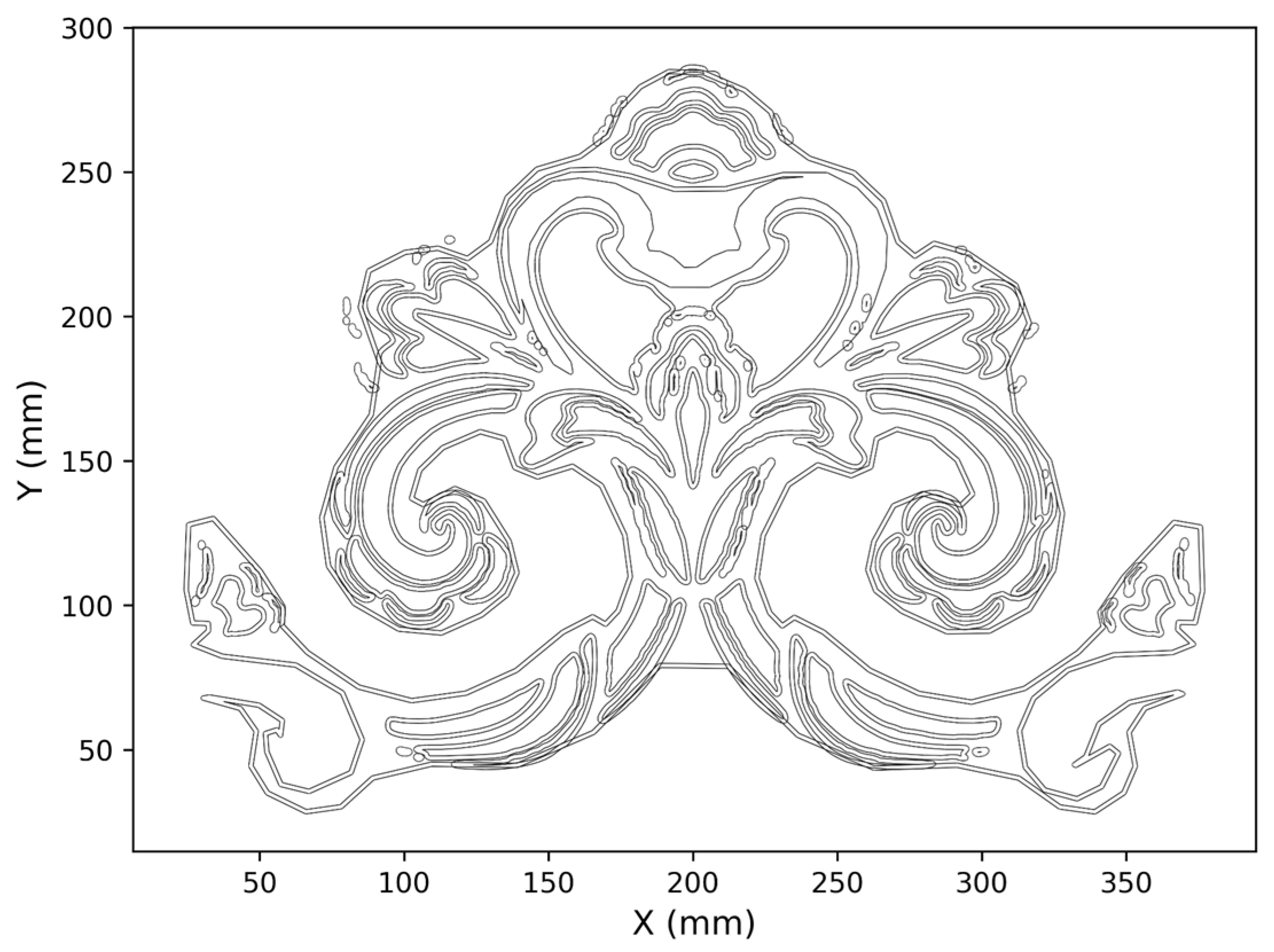
The archived Baoxianghua NC program contains 168 contour blocks, and each contour sequentially executes four cutting depths: −0.5, −1.0, −1.5, and −2.0 mm. The program is programmed in millimeters and absolute coordinates, and the nominal tool diameter marked in the file is 1.5 mm. By parsing the XY cutting instructions at the first layer Z = −0.5 mm, the X-coordinate range of the tool center path is obtained as 23.776–377.175 mm, and the Y-coordinate range is 27.750–287.150 mm; the corresponding bounding-rectangle size of the nominal toolpath is 353.399 × 259.400 mm. Figure 7 shows the XY cutting motion at Z = −0.5 mm, with coordinates in millimeters corresponding to the nominal program coordinates; the drawing line width does not represent the actual tool diameter or carved-groove width.
Figure 7.
First-layer tool center path of the archived Baoxianghua NC program.
To further quantitatively describe the above image-space correspondence, this study uses local dark-feature enhancement and threshold segmentation to extract candidate carved-groove regions from the specimen photograph (Figure 8), and obtains an image line representation through skeletonization. After completing post hoc registration, resampling is performed along the first-layer NC path at intervals of 1.6 mm in nominal program coordinates, yielding a total of 10,994 path sampling points, and the nearest Euclidean distance from each sampling point to the candidate carved-groove skeleton in the photograph is calculated. At the representative threshold T = 24, the median one-way distance from the path sampling points to the photo skeleton is 1.134 pixels, the 90th percentile is 2.724 pixels, and 93.03% of the sampling points lie within 3 pixels of the candidate skeleton. The two distances correspond to 0.436% and 1.046% of the width of the registered pattern image, respectively. A sensitivity analysis is further conducted at thresholds T = 18, 24, 30, and 36; the median distance is 1.134–1.188 pixels, and the 90th percentile is 2.724–2.917 pixels. The complete results are given in Supplementary Table S14. It should be emphasized that the above metrics are one-way image distances from the post hoc-registered program path to the candidate carved-groove skeleton in the photograph, rather than physical dimensional errors between the intended contour and the actual machined contour.
Figure 8.
Machined specimen display for the single Baoxianghua case.
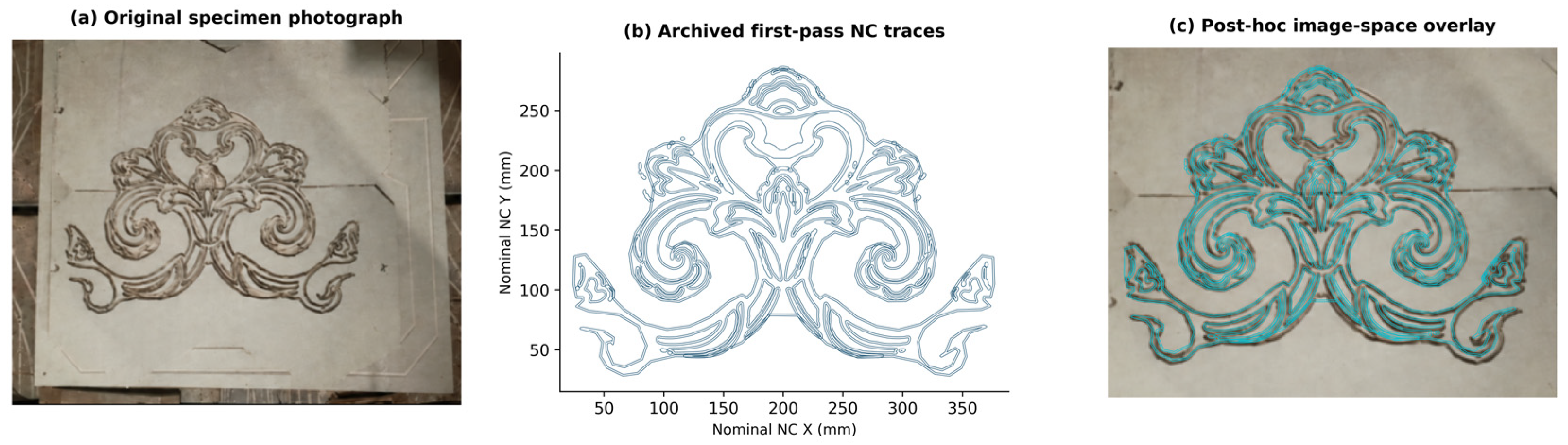
In summary, combined with the aforementioned idealized feed-time calculation and 2D tool-diameter accessibility analysis, the study can describe the geometric characteristics of the toolpath under specific inputs and established computational assumptions, but it cannot yet be used to verify the machining accuracy and general applicability of the workflow under different pattern, tool, wood, or equipment conditions.
3.7. Idealized Feed Motion Time for the Baoxianghua Motif Case
According to the position and modal feed commands in the NC file, all G01 motions across the four depth layers are accumulated. There are 97,980 planar G01 commands in total, with a cumulative path length of 70,093.66 mm, corresponding to an idealized feed time of 71.88 min; there are 672 Z-direction feeds in total, with a cumulative distance of 7560.00 mm, corresponding to 25.20 min. The subtotal of the feed motion time for the two parts is 97.08 min, as shown in Table 8 and Figure 9.
Table 8.
Breakdown of the idealized feed motion time for the archived Baoxianghua NC program.
Figure 9.
Composition of idealized feed motion time across the four depth layers of the archived NC program.
Planar feed is the main component of this time subtotal, but Z-direction motion also accounts for a non-negligible proportion. These Z-direction motions include the tool-lowering process in the program, and their cumulative travel cannot be replaced merely by the sum of the four final depths. Therefore, the planar path time of a single layer or the time containing only XY motion cannot represent the feed time of the entire archived program.
Accumulation is performed according to G01 segment lengths and effective feed values, and XY planar motion and Z-direction motion are reported separately. The calculation assumes feed per minute and does not include rapid positioning, acceleration/deceleration, controller look-ahead, spindle startup, or setup/clamping time.
The 97.08 min represents the subtotal of motion time at the specified feed rate, not a measured machine cycle. Because paired baseline programs under the same input, layer depth, feed, and motion range are lacking, this study does not report a machining time reduction ratio on this basis.
3.8. Two-Dimensional Geometric Reachability and Tool-Diameter Sensitivity
Under a fixed nominal canvas size of 400 mm, a 0.1 mm computational grid, and the foreground-removal assumption, varying the disc tool diameter yields the results shown in Table 9. When the tool diameter increases from 0.5 mm to 4.0 mm, the unreachable foreground area proportion increases from 0.006% to 19.959%.
Table 9.
Unreachable foreground area proportion under different assumed tool diameters.
Among the discrete tool diameters examined, the unreachable area proportions corresponding to 0.5–1.5 mm are all below 0.4%; when the tool diameter is 2.0 mm, this proportion increases to 1.809%, and at 3.0 mm it further increases to 16.710%. The increase between 2.0 and 3.0 mm is 14.901 percentage points, which is the interval with the largest change among the adjacent sampled tool diameters in this study. This change indicates that the current input geometry exhibits a relatively obvious ideal coverage loss within this tool-diameter range, but the limited discrete sampling cannot be used to determine an exact critical tool diameter.
Figure 10 also presents the spatial distributions under tool diameters of 1.5 mm and 4.0 mm. At 1.5 mm, the red unreachable regions are fewer and localized; at 4.0 mm, the red regions expand along multiple narrow lines and curved details. This distribution shows that the effect of increasing tool diameter on different local geometries is not uniform, and reporting only the overall area proportion cannot fully express where the loss occurs.
Figure 10.
Idealized two-dimensional geometric reachability and tool-diameter sensitivity for the Baoxianghua motif case. The left panel shows the unreachable foreground area proportion under different assumed tool diameters, where the red-brown line with dots only connects discrete computational points to indicate the trend; the middle and right panels show the spatial distributions under tool diameters of 1.5 mm and 4.0 mm, respectively. In the spatial distribution panels, the blue outlines represent the target motif contours (i.e., the intended carving paths), and the red lines indicate the geometrically unreachable areas that the tool cannot cover due to size constraints.
This calculation considers ideal coverage when all allowable tool centers can be traversed, rather than the tool sweep region actually generated by the archived NC trajectory. Therefore, the 0.396% corresponding to a 1.5 mm tool diameter cannot be interpreted as physical machining error or the actual material residual rate. The results only support a description of tool-diameter sensitivity under the current input, scale, and foreground interpretation, and do not establish a general threshold for the minimum width-to-tool-diameter ratio.
4. Discussion
4.1. Semantic–Structural Fusion Under Current Data and Training Conditions
Internal comparisons indicate that pretrained visual representations contributed the main part of the recognition performance on the current corpus. The semantic-only configuration achieved an out-of-fold macro-averaged F1 mean of 44.21%, the full model achieved 43.91%, the concatenation fusion achieved 43.20%, and the structural-only configuration achieved 2.74%. These results indicate that the benefit of combining representations depends on the discriminative information learned by each branch and on how this information enters the classifier.
The low performance of the structural-only configuration should be interpreted in light of its training conditions. Unlike the CLIP branch, the three-layer convolutional encoder is trained from scratch, with approximately 700 training images per fold covering 55 classes. The two branches therefore differ in both architecture and access to pretraining, and their performance difference cannot be attributed solely to the difference between convolutional and Transformer processing. Limited training data, optimization settings, model capacity, and normalization may all play a role, but the available experiments cannot determine their independent effects. In particular, gradient accumulation increases the number of samples involved in optimizer updates but does not increase the mini-batch used to estimate Batch Normalization statistics. This distinction points to possible factors for subsequent investigation rather than providing an established explanation of the observed performance.
The fusion results also need to be interpreted at the configuration level. The full model is 0.71 percentage points higher than the concatenation variant in mean macro-averaged F1 but still 0.30 percentage points lower than the semantic-only configuration. Its semantic skip connection provides a direct pathway from pretrained representations to the classifier, which is consistent with the full model maintaining performance close to that of the semantic branch. However, the experiments do not determine whether the learned residual contributes complementary information, compensates for optimization differences, or is largely attenuated during training. Therefore, the small difference relative to the semantic-only model should not be attributed to “noise introduced by fusion” without analyses of residual magnitude, learned scaling coefficients, or controlled branch perturbations.
The standard deviation of the full model across three seeds is smaller than that of the other configurations. However, these runs share the same frozen splits, and the full-model experiments include both CPU and GPU execution. The observed variation therefore describes the variation in repeated training under the recorded conditions rather than sensitivity to new datasets, source collections, or physical objects. Three seeds are also insufficient to establish generally stable training effects of the residual architecture.
Feature analysis provides a complementary perspective. Across the three test folds for seed 42, intra-class cosine similarities were all higher than inter-class similarities, but t-SNE projections showed substantial overlap among classes. These observations indicate that the learned features have class-related organization on average but do not prove complete class separation. They are consistent with a representation that “supports some discrimination but still leaves considerable ambiguity in the 55-class task.” Importantly, this analysis targets visual embeddings: neither local clustering nor class-center similarity can establish equivalence of cultural semantics.
Therefore, the contribution of the recognition component is an explicitly evaluated semantic–structural configuration and its internal comparison under a shared protocol. The experiments identify the importance of the pretrained visual branch and show that the proposed fusion did not consistently outperform that branch. They do not establish an advantage over an external ResNet baseline, nor do they prove that architectural complexity itself yields better pattern recognition.
4.2. Importance of Data Provenance and Grouped Evaluation
The use of 1302 known source-proxy groups addresses a specific evaluation question: identified duplicate, derivative, and other documented provenance-related images should not appear in different partitions within the same fold. This is particularly important for pattern datasets because multiple crops, photographs, or graphic reproductions may share substantial visual information. Preventing these known associations from crossing partitions improves the interpretability of the reported comparisons because all configurations are evaluated under the same documented grouping constraints.
However, the strength of grouped evaluation depends on the completeness of the grouping information. Proxy groups are not necessarily physical objects, and two unlinked records may still depict the same carving. Therefore, the non-overlap of record hashes and proxy identifiers across partitions cannot establish complete object-level independence. The results should be understood as performance under known provenance grouping rather than as a fully validated estimate of generalization to unseen objects. Because no paired comparison with an ungrouped protocol was performed, the magnitude of performance change caused by grouping is also unknown.
The long-tailed distribution further affects interpretation. Macro-averaged F1 weights each class equally, making low-performance and rare classes visible in the overall score. At the same time, estimates for classes with very few samples can change substantially when only one or two predictions differ. Therefore, reporting per-class support and performance in addition to overall metrics is necessary. The smaller seed-level standard deviation of the full model does not eliminate uncertainty in the composition and provenance of these rare classes.
The frozen-input design also separates classification evaluation from segmentation evaluation. Because the classifier uses archived offline images, its results characterize recognition performance under these input conditions. They do not quantify errors introduced when the segmentation model is applied to new photographs. In a practical system, missed regions, merged instances, incomplete boundaries, and residual background may all alter the input distribution of the classifier. An independent segmentation test set and matched downstream evaluation are needed to measure this preprocessing error propagation. The current task separation makes the reported results reproducible while clarifying the additional evidence required for end-to-end evaluation.
4.3. From Visual Relations to Manufacturing Decisions
This study distinguishes three representations that should not be interchanged: class similarity describes proximity in the learned visual space; the manufacturing graph records asserted relations among heterogeneous entities; and the CAM dictionary specifies the configuration returned for a given class key. Shared pattern names provide an interface among these representations but do not by themselves establish valid inference from visual appearance to machining conditions.
This distinction is important because visually similar patterns may have different manufacturing requirements. Tool selection and process settings depend on size, depth, material, setup, and accessible geometry, which are not determined by class-center cosine similarity. Conversely, visually different patterns may use the same machining settings. The current dictionary illustrates the latter case: Baoxianghua and the Wanzi pattern return the same default configuration. This is a transparent description of program behavior but does not provide evidence that class-related recommendations improve manufacturing outcomes.
The discrepancy between the manufacturing graph and the CAM configuration further illustrates the current implementation. The manufacturing graph associates Baoxianghua with a 0.5 mm V-shaped tool and different depth settings, whereas the archived CAM configuration uses a nominal 1.5 mm tool. These records should therefore be interpreted as independent knowledge and execution artifacts. Their coexistence indicates that explicit configuration provenance and version correspondence are required before graph-based recommendations can be described as driving the manufacturing process.
Future actionable knowledge systems need to distinguish stored relations, rule-derived recommendations, operator-approved configurations, and executed programs. Validation would then examine whether recommendations are appropriate and whether they improve specific outcomes relative to transparent alternatives. Listing graph entities and inspecting relation paths are necessary for traceability but cannot replace independent expert judgment or controlled manufacturing comparisons. Therefore, the current contribution is a documented knowledge representation and an inspectable configuration interface, not a validated manufacturing recommendation system.
The new computational analyses reinforce the geometric description of the case while answering different questions. The 97.08 min feed motion subtotal describes the cumulative contribution of programmed G01 motion under an assumed feed interpretation. It does not predict the complete machine cycle because rapid moves, acceleration, controller behavior, and auxiliary operations are excluded. Its value lies in making the scope of the time calculation explicit (including repeated depth passes and Z-axis approaches) rather than in establishing a machining time reduction.
Similarly, the 2D reachability computation identifies where a circular tool can cover the assumed removal region if all allowable tool-center positions are traversed. The unreachable area increases from 1.809% at a 2.0 mm diameter to 16.710% at 3.0 mm, revealing a significant scale-dependent change for this specific binary geometry. It does not establish a universal tool-diameter threshold, nor does it describe the material actually removed by the archived trajectory. A smaller unreachable area percentage also does not necessarily imply acceptable preservation: a small affected area may contain visually or culturally important details. Therefore, in heritage applications, area-based reachability should be supplemented by feature-level inspection.
4.4. Establishing Architectural Relevance Through Contextualized Pattern Records
The architectural relevance of this work lies in the relationship between decorative patterns and their host components. Cao and Mustafa’s study of Huizhou doors and windows identified regional characteristics of carving practices and their locations; Zhao et al. examined associations between window lattice patterns and architectural positions [43,44]. These studies support treating patterns as part of spatial and tectonic context rather than as isolated image categories.
Yusof et al.’s study of Johor Malay houses provides a relevant perspective, documenting woodcarving locations and design composition types as elements of regional architectural identity [45]. This suggests that recognition records intended for architectural use should link images to their buildings, components, locations, and provenance documents. Predicted categories can assist such records but cannot determine whether a pattern is historically appropriate at a specific architectural location.
This contextual requirement also changes how digital reproduction is evaluated. Guo and Sahari’s analysis of Dongyang woodcarving discussed threats such as symbolic change, aesthetic simplification, and detachment from cultural context [46]. Interpreted together with the geometric analysis in this paper, this highlights the distinction between “making shapes machinable” and “preserving their heritage meaning”. Tool-compatible contours may still omit meaningful features or reproduce patterns in inappropriate contexts. Current classification and reachability metrics do not measure these dimensions of authenticity.
Within these limitations, the workflow has three potential architectural uses. For documentation, category predictions and visual feature relationships can assist manual cataloging and candidate retrieval within archives. Given the current recognition performance, these outputs should be reviewed by experts rather than automatically populate authoritative heritage records. Building and component identifiers can also link multiple views and support more defensible object-level evaluation.
For restoration preparation, when original photographs, measured drawings, or reliably associated samples already provide evidence of the intended form, contour processing can serve as a geometric starting point. It cannot infer missing geometry solely from a class label. The 2D reachability map can then help identify details requiring smaller tools, different processes, or manual finishing, but these choices still need to be checked against component dimensions, material condition, and conservation objectives. This study did not validate these decisions on architectural components.
For contemporary design, recognized pattern categories can provide retrieval paths to existing decorative samples. Their reuse needs to consider cultural meaning, regional provenance, composition, and intended architectural setting. Visual similarity should not be regarded as evidence that patterns from different contexts are interchangeable.
The current Baoxianghua case involves geometry derived from planar images and layered contour paths. It does not cover depth reconstruction of complex reliefs, mortise-and-tenon joints in assembled latticework, structural behavior, or installation tolerances. Therefore, the architectural transfer proposed here is specific: it assists pattern documentation and part of geometric preparation tasks, followed by component-level design and validation. It is not a proven substitute for architectural surveying, conservation judgment, or craft expertise.
4.5. Limitations
The main limitations concern both the coverage of evidence and the correspondence among stages. Historical image provenance remains incomplete, physical object independence has not been fully established, and the segmentation module lacks an independent test set. The recognition experiments used a single corpus, three fixed folds, and three training seeds; their results do not establish performance on new cases. Mixed CPU and GPU execution further limits interpreting the observed variation as a pure random-seed effect.
The manufacturing graph has not been independently evaluated for recommendation quality, and the computational manufacturing analysis introduces additional assumptions. The reachability results depend on the binarization of low-resolution images, their nominal 400 mm canvas width, the interpretation of foreground as material to be removed, and a 0.1 mm grid. Resampling cannot recover geometric details absent from the source image. Grid convergence and alternative segmentation or scaling conditions were not examined. Moreover, at the manufacturing level, graph recommendations should be compared with fixed default configurations and independent process decisions under identical input conditions.
Further work should prioritize strengthening correspondence and independent evaluation. At the data level, physical object identity and view relationships should be established before constructing object-level or collection-level held-out tests. Segmentation should be evaluated using an independently annotated mask set, followed by classification evaluation on the corresponding predicted regions. At the model level, controlled comparisons of pretraining, normalization, and fusion behavior can help explain the weaker structural-only results and the conditional value of fusion.
5. Conclusions
This paper addresses traditional woodcarving patterns and establishes and evaluates a modular workflow comprising semantic–structural recognition and downstream geometric toolpath construction. The research contributions are reflected in the unified grouped evaluation of a 55-class corpus, the empirical comparison of four recognition configurations, the explicit separation of manufacturing relations from actual configurations, and the program and geometric analysis of a single case.
Across 36 runs involving 1373 formal samples, three seeds, and three folds, the mean Macro-F1 values of the semantic-only branch, the full model, the concatenation mapping, and the structural-only branch were 44.21%, 43.91%, 43.20%, and 2.74%, respectively. This comparison establishes the pretrained semantic configuration as a strong reference for the current task and shows that the current structural branch and residual fusion have not yet yielded consistent additional classification benefits. In all three test folds, sample-level intra-class similarity was higher than inter-class similarity, providing a complementary description of the class-related organization of the features. In the manufacturing part, relation examples of five entity types and class-configuration queries clarify the interface between knowledge organization and program parameters. For the Baoxianghua case, the subtotal of the archived NC feed motion time is 97.08 min; an independent two-dimensional analysis shows that the unreachable foreground area proportions corresponding to assumed tool diameters of 1.5 mm and 4.0 mm are 0.396% and 19.959%, respectively. These results provide inspectable program characteristics and tool-diameter sensitivity information, while the physical photographs provide a qualitative machining demonstration.
This paper provides comparative evidence for domain-specific data and a single-case geometric computation workflow, which can serve as a reference for the cataloging, retrieval, and geometric machining preparation of architectural woodcarving patterns; restoration of architectural components, the benefit of independent recommendations, and physical machining accuracy still require further validation.
Supplementary Materials
The following supporting information can be downloaded at: https://www.mdpi.com/article/10.3390/buildings16224559/s1. Figure S1: Feature analysis of the full model on the fold 2 test set for seed 42. Including 457 test features; (a) t-SNE projection; (b) class-center cosine similarity matrix. The computational and color-coding descriptions are the same as in Figure 5; Figure S2: Feature analysis of the full model on the fold 3 test set for seed 42. Including 458 test features; (a) t-SNE projection; (b) class-center cosine similarity matrix. Features were extracted using the corresponding encoder for each fold; Table S1: Consolidated Annotation, Ambiguity, and Adjudication Protocol; Table S2: Recording Requirements and Statistical Usability for Annotation Quality Control; Table S3: Formal samples of 55 classes and three-fold details; Table S4: Classification training parameters; Table S5: Archived Configuration of the Preprocessing Segmentation Tool; Table S6: Manufacturing Graph Entity List; Table S7: List of Directed Relations in the Manufacturing Graph; Table S8: Path Retrieval and Configuration Comparison for the Baoxianghua and Wanzi Classes; Table S9: Transparent Default Configuration Comparison; Table S10: Class-level support and pooled out-of-fold F1 scores; Table S11: Complete fold-level results for four model configurations (36 runs); Table S11-A: Pooled out-of-fold metrics by random seed; Table S12: Frozen sample-level manifest and grouped evaluation audit; Table S13: Provenance and source-stratified counts of initial and retained records; Table S13a: Final disposition of the 17 records not accounted for by the three exclusion categories; Table S14: Sensitivity analysis of NC-to-photo skeleton distance for the Baoxianghua pattern with respect to the image extraction threshold.
Author Contributions
X.Y. and J.L.; methodology, X.Y.; software, X.Y.; validation, X.Y. and J.L.; formal analysis, X.Y.; investigation, X.Y.; resources, X.Y.; data curation, X.Y.; writing—original draft preparation, X.Y.; writing—review and editing, J.L.; visualization, X.Y.; supervision, J.L.; project administration, X.Y.; funding acquisition, J.L. All authors have read and agreed to the published version of the manuscript.
Funding
This research was funded by the 2023 Social Science Foundation of Jiangsu Province, “Research on the Construction of Collaborative Innovation Ecosystem of Jiangnan Traditional Handicrafts” (23YSC008), and the 2025 Jiangsu Provincial Postgraduate Research and Innovation Programme (KYCX25_1482). The APC was not applicable.
Institutional Review Board Statement
Not applicable.
Informed Consent Statement
Not applicable.
Data Availability Statement
The data supporting this study are available from the corresponding author upon reasonable request. Specifically, de-identified sample manifests (including sample IDs, class labels, proxy-group IDs, and fold assignments) and cross-subset overlap check reports are provided in Supplementary Files (Table S12). Source-stratified counts and record-level disposition lists (Tables S13 and S13a) are provided in the Supplementary Materials. Aggregated performance metrics, out-of-fold model predictions, and the CAM configuration dictionaries are available upon request. The source code used for the analysis and the geometric toolpath generation scripts are also available upon request. Original enterprise images and archival materials are not publicly released due to copyright and confidentiality restrictions (as detailed in Supplementary Table S13); however, authorization documentation and original file paths are provided exclusively for editorial verification.
Acknowledgments
The authors would like to thank the anonymous reviewers for their constructive comments, which helped improve the quality of this manuscript. We also sincerely thank the leaders and teachers from the College of Furnishings and Industrial Design at Nanjing Forestry University for their help and support.
Conflicts of Interest
The authors declare no conflicts of interest.
References
- Adane, A.; Chekole, A.; Gedamu, G. Cultural heritage digitization: Challenges and opportunities. Int. J. Comput. Appl. 2019, 178, 1–5. [Google Scholar] [CrossRef] [Scilit]
- Manžuch, Z. Ethical issues in digitization of cultural heritage. J. Contemp. Arch. Stud. 2017, 4, 4. [Google Scholar]
- Xia, X.; Chen, Z.; Xu, Y. Digital restoration and feature recognition of a Qing-Dynasty vernacular dwelling based on multimodal data fusion. Sci. Rep. 2025, 16, 1844. [Google Scholar] [CrossRef] [Scilit]
- Iakovaki, E.; Makris, D.; Malea, E. Digital Documentation and Reconstruction of Fragile Organic Artefacts: A State-of-the-Art Review. Int. Arch. Photogramm. Remote Sens. Spat. Inf. Sci. 2025, 48, 607–614. [Google Scholar] [CrossRef] [Scilit]
- Gao, L.; Wu, Y.; Yang, T.; Zhang, X.; Zeng, Z.; Chan, C.K.D.; Chen, W. Research on image classification and retrieval using deep learning with attention mechanism on diaspora Chinese architectural heritage in Jiangmen, China. Buildings 2023, 13, 275. [Google Scholar] [CrossRef] [Scilit]
- Wang, M.; Lau, N. NFT digital twins: A digitalization strategy to preserve and sustain Miao silver craftsmanship in the metaverse era. Heritage 2023, 6, 1921–1941. [Google Scholar] [CrossRef] [Scilit]
- Zhou, G.; Zhang, C.; Li, Z.; Ding, K.; Wang, C. Knowledge-driven digital twin manufacturing cell towards intelligent manufacturing. Int. J. Prod. Res. 2020, 58, 1034–1051. [Google Scholar] [CrossRef] [Scilit]
- Guo, P.; Wu, Y.; Shen, Z.; Zhang, H.; Zhang, P.; Lou, F. A smoothing method of continuous line-segment path in CNC machining based on real-time transformation of interpolation points. Int. J. Adv. Manuf. Technol. 2022, 118, 4043–4054. [Google Scholar] [CrossRef] [Scilit]
- Zhao, Y.; Liu, Q.; Xu, W.; Yuan, H.; Lou, P. An ontology self-learning approach for CNC machine capability information integration and representation in cloud manufacturing. J. Ind. Inf. Integr. 2022, 25, 100300. [Google Scholar] [CrossRef] [Scilit]
- Islami, F.; Sutanto, A. Digitalization of Design and Machining Processes of Wood Carving Products Using CAD/CAM/CNC Technologies for Preservation of Minangkabau Culture. J. Ocean Mech. Aerosp. Sci. Eng. 2024, 68, 127–132. [Google Scholar] [CrossRef] [Scilit]
- Scopigno, R.; Cignoni, P.; Pietroni, N.; Callieri, M.; Dellepiane, M. Digital Fabrication Technologies for Cultural Heritage (STAR). In Proceedings of the Eurographics Workshop on Graphics and Cultural Heritage; GCH ’14; Eurographics Association: Darmstadt, Germany, 2014; pp. 75–85. [Google Scholar]
- Medjadi, M.; Meddeber, L.; Zouagui, T. Enhancing building extraction from remote sensing images using YOLOV8. In 2024 2nd International Conference on Electrical Engineering and Automatic Control (ICEEAC); IEEE: New York, NY, USA, 2024; pp. 1–6. [Google Scholar]
- Zhong, H.; Zhang, Z.; Liu, H.; Wu, J.; Lin, W. Individual tree species identification for complex coniferous and broad-leaved mixed forests based on deep learning combined with UAV LiDAR data and RGB images. Forests 2024, 15, 293. [Google Scholar] [CrossRef] [Scilit]
- Lin, T.Y.; Goyal, P.; Girshick, R.; He, K.; Dollár, P. Focal loss for dense object detection. In Proceedings of the IEEE International Conference on Computer Vision, Honolulu, Hawaii, 21–26 July 2017; pp. 2980–2988. [Google Scholar]
- Cui, Y.; Jia, M.; Lin, T.Y.; Song, Y.; Belongie, S. Class-balanced loss based on effective number of samples. In Proceedings of the IEEE/CVF Conference on Computer Vision and Pattern Recognition, Long Beach, CA, USA, 16–20 June 2019; pp. 9268–9277. [Google Scholar]
- Li, Z.; Zhao, H.; Lin, Y. Multi-task convolutional neural network with coarse-to-fine knowledge transfer for long-tailed classification. Inf. Sci. 2022, 608, 900–916. [Google Scholar] [CrossRef] [Scilit]
- Liu, L.; Qiu, J.; Cao, Y.; Li, Q.; Qian, S.; Sun, Y. An interpretable approach to wood species identification based on anatomical features in microscopic images. Forests 2025, 16, 1328. [Google Scholar] [CrossRef] [Scilit]
- Ye, S.; Chen, S.; Wang, R.; Wu, T.; Xu, J.; Khan, S.; Khan, F.S.; Shao, L. Concept Drift and Long-Tailed Distribution in Fine-Grained Visual Categorization: Benchmark and Method. Proc. IEEE Trans. Pattern Anal. Mach. Intell. 2026, 48, 8970–8986. [Google Scholar] [CrossRef] [Scilit]
- Rodríguez-De-Vera, J.M.; Estepa, I.G.; Bolaños, M.; Bolaños, M.; Nagarajan, B.; Radeva, P. LOFI: LOng-tailed FIne-grained network for food recognition. In Proceedings of the IEEE/CVF conference on computer vision and pattern recognition, Seattle, WA, USA, 17–18 June 2024; pp. 3750–3760. [Google Scholar]
- Radford, A.; Kim, J.W.; Hallacy, C.; Ramesh, A.; Goh, G.; Agarwal, S.; Sastry, G.; Askell, A.; Mishkin, P.; Krueger, G.; et al. Learning transferable visual models from natural language supervision. In Proceedings of the 38th International Conference on Machine Learning, Virtual, 18–20 July 2021; PMLR. pp. 8748–8763. [Google Scholar]
- Zhou, K.; Yang, J.; Loy, C.C.; Liu, Z. Learning to prompt for vision-language models. Int. J. Comput. Vis. 2022, 130, 2337–2348. [Google Scholar] [CrossRef] [Scilit]
- Zhu, L.; Wang, X.; Feng, J.; Cheng, T.; Li, Y.; Jiang, B.; Zhang, D.; Han, J. Weakclip: Adapting clip for weakly-supervised semantic segmentation. Int. J. Comput. Vis. 2025, 133, 1085–1105. [Google Scholar] [CrossRef] [Scilit]
- Jia, C.; Yang, Y.; Xia, Y.; Chen, Y.; Parekh, Z.; Pham, H.; Le, Q.V.; Sung, Y.; Li, Z.; Duerig, T. Scaling up visual and vision-language representation learning with noisy text supervision. In Proceedings of the International Conference on Machine Learning, Virtual, 18–24 July 2021; PMLR. pp. 4904–4916. [Google Scholar]
- Sun, S.; Yu, D.; Wang, C.; Xie, C. A smooth tool path generation and real-time interpolation algorithm based on B-spline curves. Adv. Mech. Eng. 2018, 10, 1687814017750281. [Google Scholar] [CrossRef] [Scilit]
- Chaikin, G.M. An algorithm for high-speed curve generation. Comput. Graph. Image Process. 1974, 3, 346–349. [Google Scholar] [CrossRef] [Scilit]
- Xu, Y.; Mohd Zaman, M.H.; Zhou, F. Optimized continuous small line interpolation algorithm for high end CNC machine tools using a cross segment approach. Sci. Rep. 2025, 16, 1133. [Google Scholar] [CrossRef] [Scilit]
- Wu, L.; Lyu, H.; Xu, J.; Sun, Y. SBQI: A smooth b-spline-based quaternion interpolation method for C3-continuous tool orientation planning in 5-axis CNC machining. Int. J. Adv. Manuf. Technol. 2026, 142, 851–868. [Google Scholar] [CrossRef] [Scilit]
- Wang, Z.; Wang, X.; Wang, Y.; Wang, R.; Bao, M.; Lin, T.; He, P. Ball end mill—Tool radius compensation of complex NURBS surfaces for 3-axis CNC milling machines. Int. J. Precis. Eng. Manuf. 2020, 21, 1409–1419. [Google Scholar] [CrossRef] [Scilit]
- Szaroleta, M.; Treter, G.; Nowak, K. Modified tool radius compensation in the Archimedes’ spiral tool path for high speed machining of circular geometry. J. Manuf. Process. 2023, 97, 275–289. [Google Scholar] [CrossRef] [Scilit]
- Zhao, H.; Zhu, L.M.; Ding, H. A real-time look-ahead interpolation methodology with curvature-continuous B-spline transition scheme for CNC machining of short line segments. Int. J. Mach. Tools Manuf. 2013, 65, 88–98. [Google Scholar] [CrossRef] [Scilit]
- Guo, L.; Yan, F.; Li, T.; Yang, T.; Lu, Y. An automatic method for constructing machining process knowledge base from knowledge graph. Robot. Comput.-Integr. Manuf. 2022, 73, 102222. [Google Scholar] [CrossRef] [Scilit]
- Xiao, Y.; Zheng, S.; Leng, J.; Gao, R.; Fu, Z.; Hong, J. An assembly process planning pipeline for industrial electronic equipment based on knowledge graph with bidirectional extracted knowledge from historical process documents. J. Intell. Manuf. 2025, 36, 3647–3667. [Google Scholar] [CrossRef] [Scilit]
- Gao, Y.; Qin, B.; Chen, F.; Huang, X.; Wu, J.; Wu, Y. Performance Evaluation of the CLIP Model in Classification Tasks. In 2025 IEEE International Conference on Systems, Man, and Cybernetics (SMC); IEEE: New York, NY, USA, 2025; pp. 3230–3235. [Google Scholar]
- Yaseen, M. What is YOLOv9: An in-depth exploration of the internal features of the next-generation object detector. arXiv 2024, arXiv:2409.07813. [Google Scholar]
- Liu, Y.; Yang, L.; Wang, Y. Long-Tailed Classification with Multi-Granularity Semantics. In Proceedings of the IEEE/CVF International Conference on Computer Vision, Honolulu, HI, USA, 19–25 October 2025; pp. 4285–4294. [Google Scholar]
- Li, X.L.; Liang, P. Prefix-tuning: Optimizing continuous prompts for generation. In Proceedings of the 59th Annual Meeting of the Association for Computational Linguistics and the 11th International Joint Conference on Natural Language Processing (Volume 1: Long Papers); Association for Computational Linguistics: Stroudsburg, PA, USA, 2021; pp. 4582–4597. [Google Scholar]
- Hu, E.J.; Shen, Y.; Wallis, P.; Allen-Zhu, Z.; Li, Y.; Wang, S.; Wang, L.; Chen, W. Lora: Low-rank adaptation of large language models. In Proceedings of the International Conference on Learning Representations (ICLR), Virtual, 25–29 April 2022; Volume 1, p. 3. [Google Scholar]
- Houlsby, N.; Giurgiu, A.; Jastrzebski, S.; Morrone, B.; de Laroussilhe, Q.; Gesmundo, A.; Attariyan, M.; Gelly, S. Parameter-efficient transfer learning for NLP. In Proceedings of the International Conference on Machine Learning, Long Beach, CA, USA, 9–15 June 2019; PMLR. pp. 2790–2799. [Google Scholar]
- Ladj, A.; Wang, Z.; Meski, O.; Belkadi, F.; Ritou, M.; Da Cunha, C. A knowledge-based Digital Shadow for machining industry in a Digital Twin perspective. J. Manuf. Syst. 2021, 58, 168–179. [Google Scholar] [CrossRef] [Scilit]
- Hoang, D.; Gorsich, D.; Castanier, M.P.; Imani, F. Knowledge graph fusion with large language models for accurate, explainable manufacturing process planning. Int. J. Prod. Econ. 2026, 300, 110091. [Google Scholar] [CrossRef] [Scilit]
- Marinov, M.; Benkhedda, Y.; Hannaford, E.D.; Alexander, M.; Nenadic, G.; Batista-Navarro, R. Relation extraction for constructing knowledge graphs: Enhancing the searchability of community-generated digital content (CGDC) collections. In Proceedings of the Workshop on Deep Learning and Large Language Models for Knowledge Graphs, Barcelona, Spain, 25–26 August 2024. [Google Scholar]
- Yan, G.; Zhang, D.; Xu, J.; Sun, Y. A C3 continuous double circumscribed corner rounding method for five-axis linear tool path with improved kinematics performance. J. Comput. Des. Eng. 2023, 10, 1490–1506. [Google Scholar] [CrossRef] [Scilit]
- Cao, Z.; Mustafa, M.B. A study of ornamental craftsmanship in doors and windows of Hui-style architecture: The Huizhou three carvings (brick, stone, and wood carvings). Buildings 2023, 13, 351. [Google Scholar] [CrossRef] [Scilit]
- Zhao, H.; He, L.; Cao, R.; Lu, Y. From Pattern to Position: Identifying Spatial Configuration Logic of Traditional Window Lattice Patterns in Zhaoyu Ancient City, China. Buildings 2026, 16, 3395. [Google Scholar] [CrossRef] [Scilit]
- Yusof, H.; Ibrahim, F.K.; Shahminan, R.N.R. Heritage identity conservation of the woodcarving placement and design composition typologies on Johor Malay houses. Plan. Malays. 2020, 18, 12–23. [Google Scholar] [CrossRef] [Scilit]
- Guo, X.; Sahari, F. Authenticity in crisis: Structural tensions and challenges in the heritage preservation of Dongyang woodcarving. J. Chin. Archit. Urban. 2026, 8, 060013. [Google Scholar] [CrossRef] [Scilit]
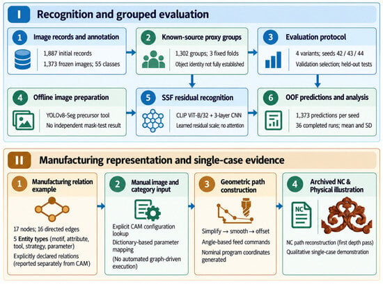
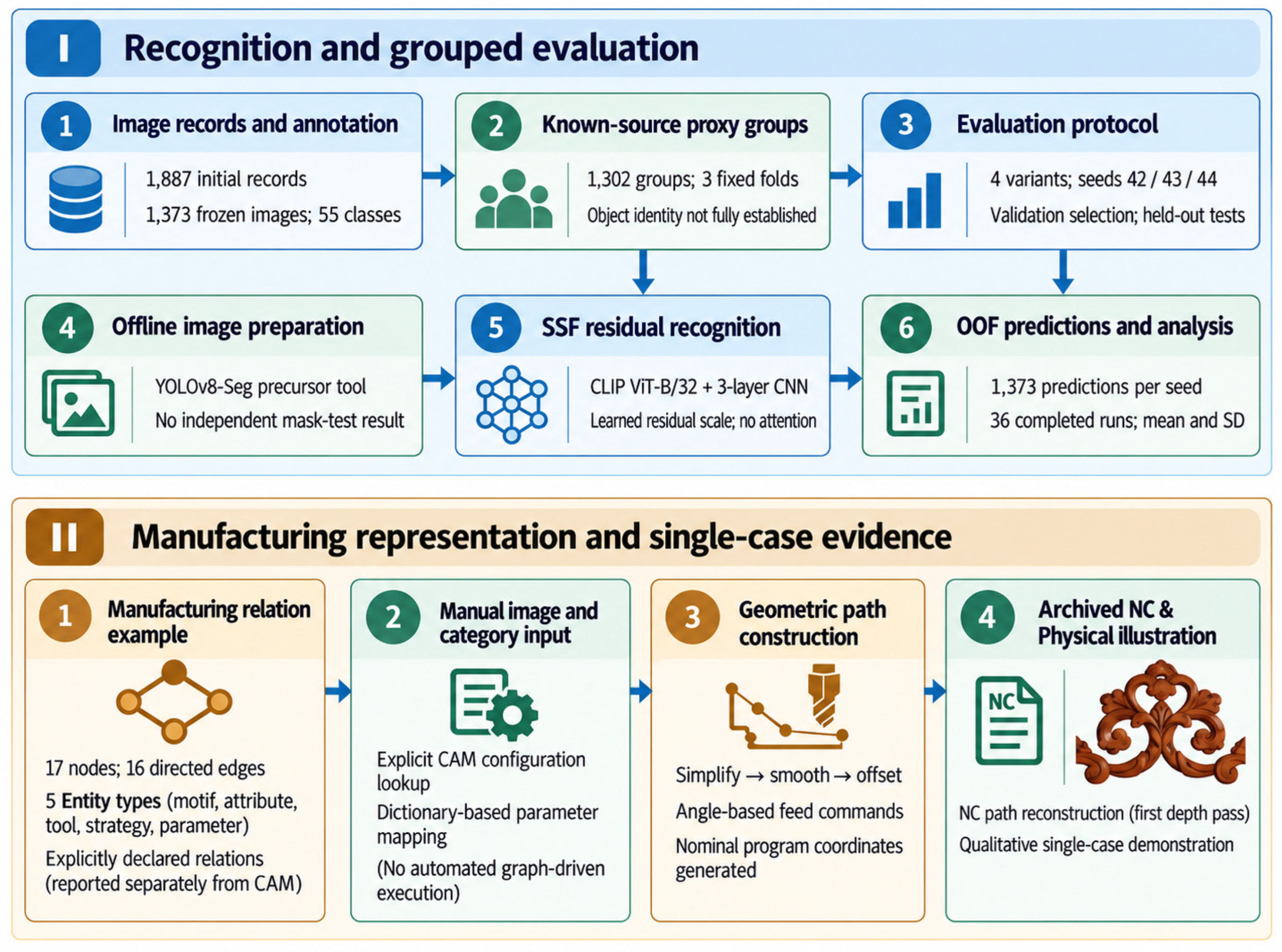
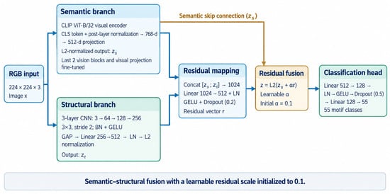
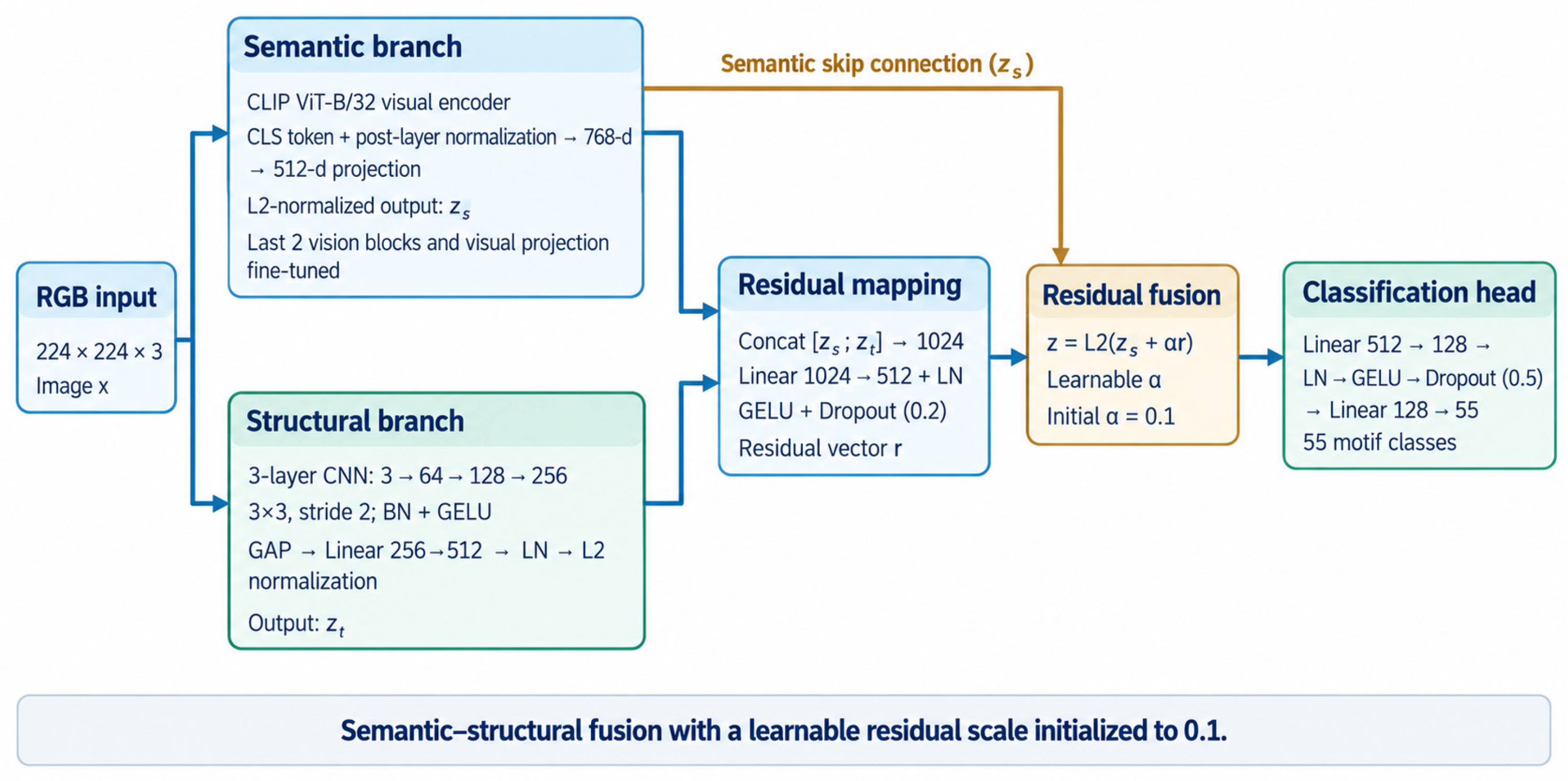
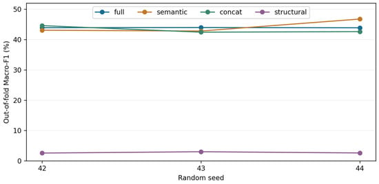
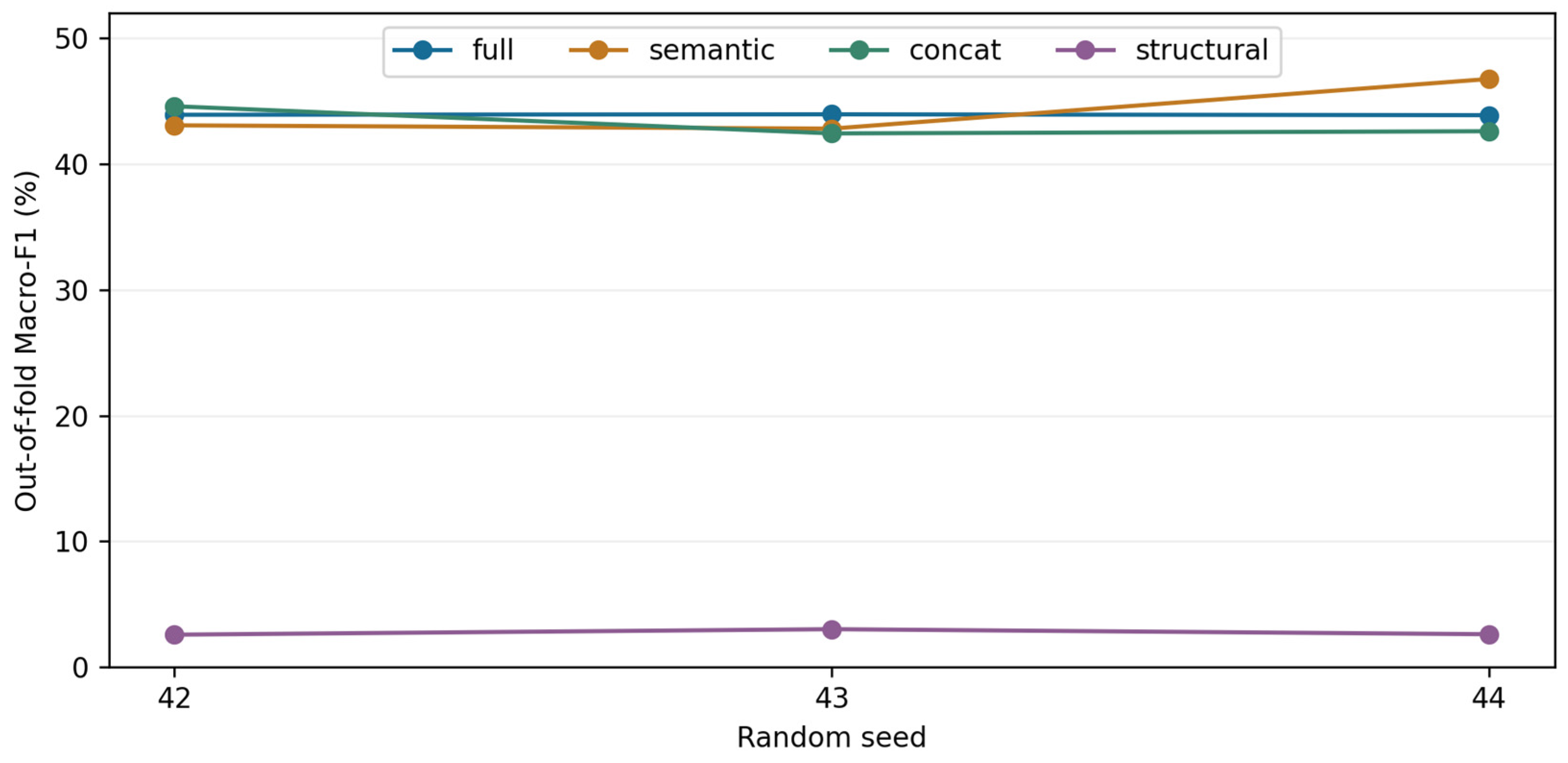
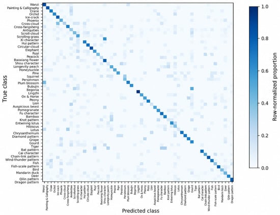
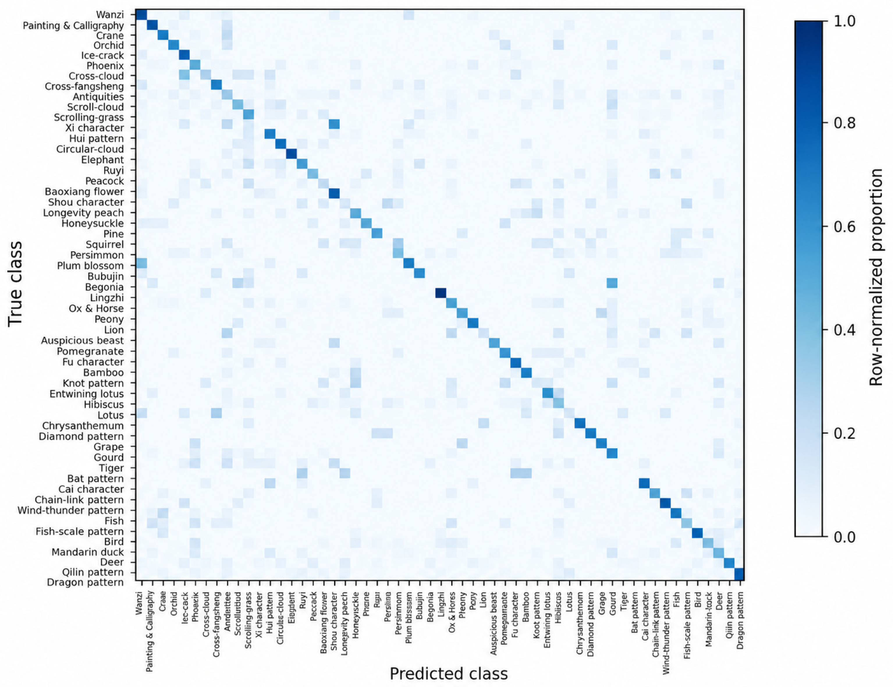
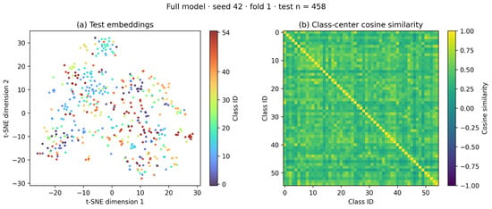
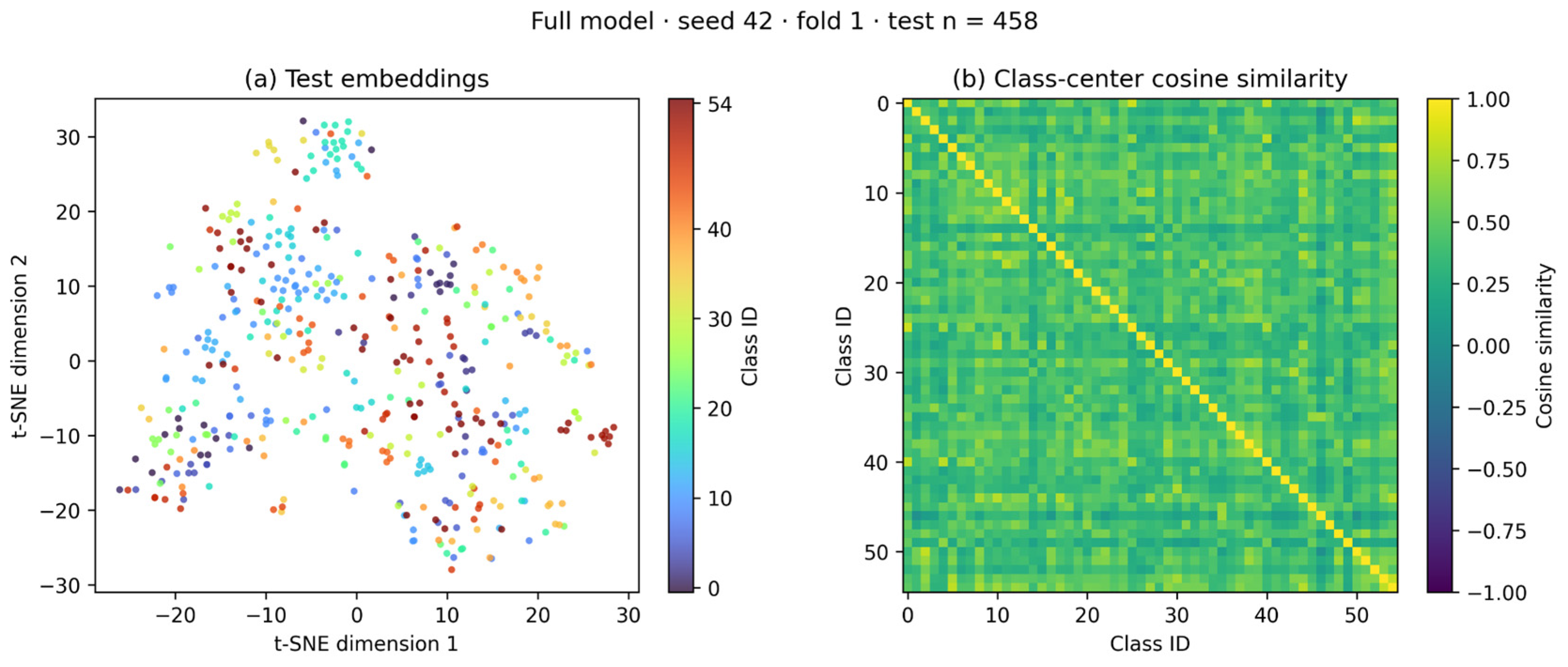
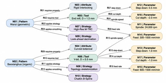
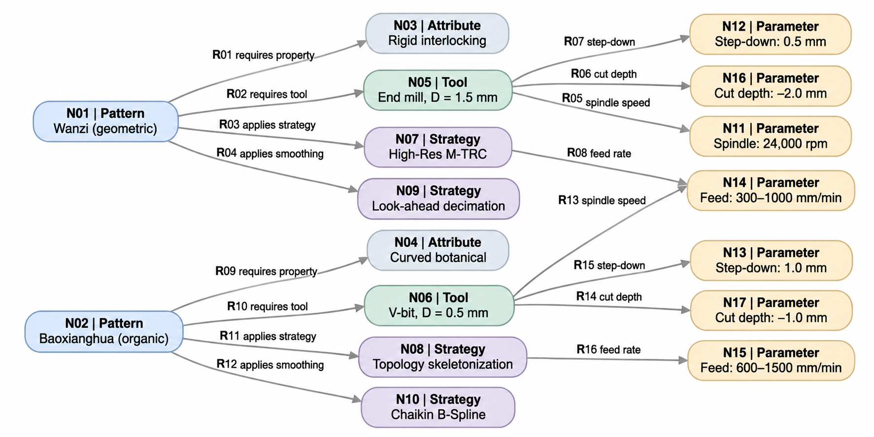
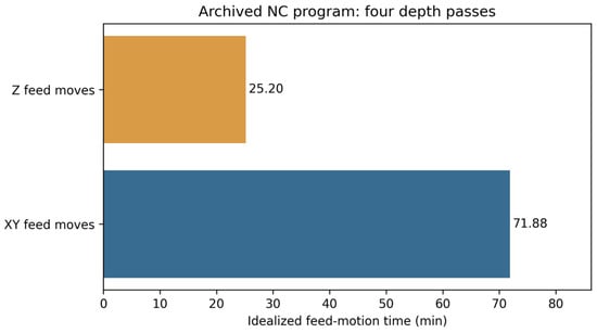
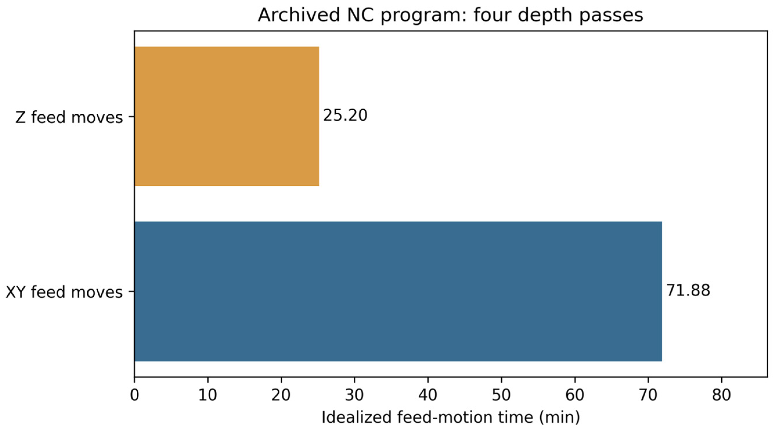
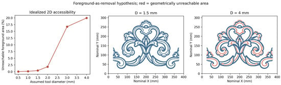
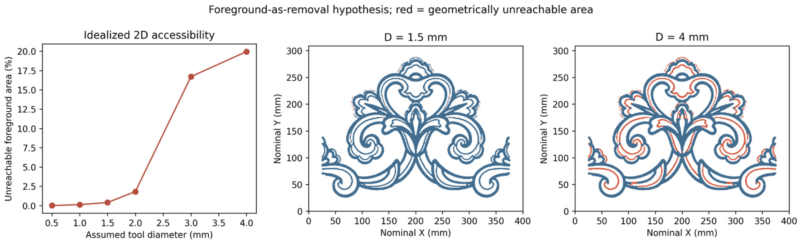

Disclaimer/Publisher’s Note: The statements, opinions and data contained in all publications are solely those of the individual author(s) and contributor(s) and not of MDPI and/or the editor(s). MDPI and/or the editor(s) disclaim responsibility for any injury to people or property resulting from any ideas, methods, instructions or products referred to in the content. |
© 2026 by the authors. Licensee MDPI, Basel, Switzerland. This article is an open access article distributed under the terms and conditions of the Creative Commons Attribution (CC BY) license.