


Abstract
Traditional earthen dwellings combine recurring architectural patterns with differences in geometry, openings, and spatial organization. This study links an architectural inventory with an exploratory numerical characterization in Sacapalca, Ecuador. Of 75 documented dwellings, 40 retained traditional characteristics and were organized into five groups; an independent analysis of 13 bioclimatic descriptors selected one medoid per group. For these five dwellings, whole-dwelling mean air temperature and relative humidity were simulated under two prescribed daily scenarios, with scheduled ventilation in the warm scenario and infiltration only in the cold scenario, using a generated weather file. Under these modeling assumptions, simulated daily air temperature amplitudes ranged from 5.33 °C to 7.00 °C in the warm scenario and from 3.23 °C to 6.41 °C in the cold scenario. No record exceeded the upper thermal reference; lower deviations depended on the case and scenario. Vapor-pressure and absolute-humidity indicators derived from the aggregated outputs complemented the temperature results with a diagnostic of moisture conditions. These values are read as relative responses under common conditions, not as predictions for the actual dwellings. The study proposes an explicit procedure for selecting observed configurations and characterizes their response under common conditions.
1. Introduction
Vernacular architecture around the world records local responses to available materials, construction knowledge, topography, and patterns of use. Its study can be understood as dynamic, since each place has a construction history, and uncovering that history can contribute to current discussions on building adaptation and heritage conservation, provided that observed features are distinguished from performance claims, which require direct measurement or validated simulation [1]. Research on traditional housing has examined passive design, envelope construction, and spatial organization as factors that can modify indoor conditions [2,3]. These studies show that a strategy cannot be transferred from one region or building type to another without contextual evidence, hence the importance of highlighting the construction responses of different localities, including the most remote or smallest ones.
The literature associates indoor thermal regulation with orientation, compactness, wall thickness, thermal mass, roof configuration, openings, shading devices, and natural ventilation [4,5,6,7,8]. This association has been studied in very different climates and with varied methods. In Cyprus, natural ventilation was analyzed as a cooling strategy in rural architecture [4], and the effect of night ventilation on comfort in vernacular buildings was assessed numerically [5]. Other studies monitored the hygrothermal behavior of adobe structures [6], compared room orientations in a hot-humid climate [7], and analyzed passive heat-protection design in Lingnan buildings [8]. These studies highlight bioclimatic strategies and help explain why traditional responses work without complex, energy-intensive systems, a knowledge that stems from construction tradition and from experience transmitted over the years.
Vernacular architecture is built from its surroundings and is refined through the decisions that shaped its design, even in environments with particular climatic conditions, although it should be kept in mind that this type of construction system has limitations. In the Ecuadorian Andes, for example, temperature and relative humidity have been monitored in rural dwellings above 3000 m a.s.l. [9], traditional earthen buildings have been simulated [10], and a rural dwelling of concrete block with a zinc roof has been compared with a traditional one with exposed thermal mass [11]. Traditional or neo-vernacular dwellings can achieve stable indoor temperatures, but comfort is often only partial in cold high-altitude conditions, and envelope insulation, bioclimatic design, and construction quality influence the outcome [9]. Several studies still report rooms outside the comfort range or benefits that depend on later improvements [2,10,12].
The passive strategies described in these cases can be complemented with new technological criteria, to improve the response to the environment of new buildings that replace or are integrated into existing built environments. In this sense, documenting vernacular architecture in remote areas is justified by the fact that cities are being renewed and require solutions suited to current sustainability approaches. There is also a risk of losing this historical technological knowledge as traditional construction methods are replaced by materials with higher embodied energy [13]. This replacement advances more slowly in rural settlements, where vernacular forms, materials, and techniques may persist for longer [14,15].
In Ecuador, studies on the environmental performance of vernacular architecture have concentrated on central Andean contexts, such as Ambato [10] and Cotopaxi [12], and on the coast [3], while settlements in the south are comparatively underrepresented. The closest southern precedent is a courtyard house in the historic center of Azogues [2], an urban setting, and in the city of Cuenca the evolution of embodied energy in Andean housing has been studied [13]. Further south, there are settlements that preserve their traditional architecture, although in contexts that are moving toward new forms and construction technologies. These settlements nonetheless allow us to learn about the role of vernacular construction systems in moderating indoor conditions under their particular climatic configuration.
Sacapalca, a rural parish in the Gonzanamá canton, Loja Province, Ecuador, is an example of such settlements, where a group of dwellings retains earth-based walls, timber elements, and spatial arrangements associated with regional building traditions. The present study broadens the geographical knowledge base with a case from the southern Andes in which these characteristics have been preserved.
This study links the architectural inventory of Sacapalca with an exploratory numerical characterization of five selected dwellings. Its objectives are to describe five architectural groups, to select a central configuration within each group using bioclimatic attributes, and to examine the air temperature and relative humidity response of each dwelling as a whole under two prescribed daily scenarios. The study does not aim to identify an optimal typology or to rank dwellings by technological superiority. The analysis presents the common architectural and bioclimatic characteristics and examines how the overall configuration of each selected dwelling responds under common simulated conditions.
2. Materials and Methods
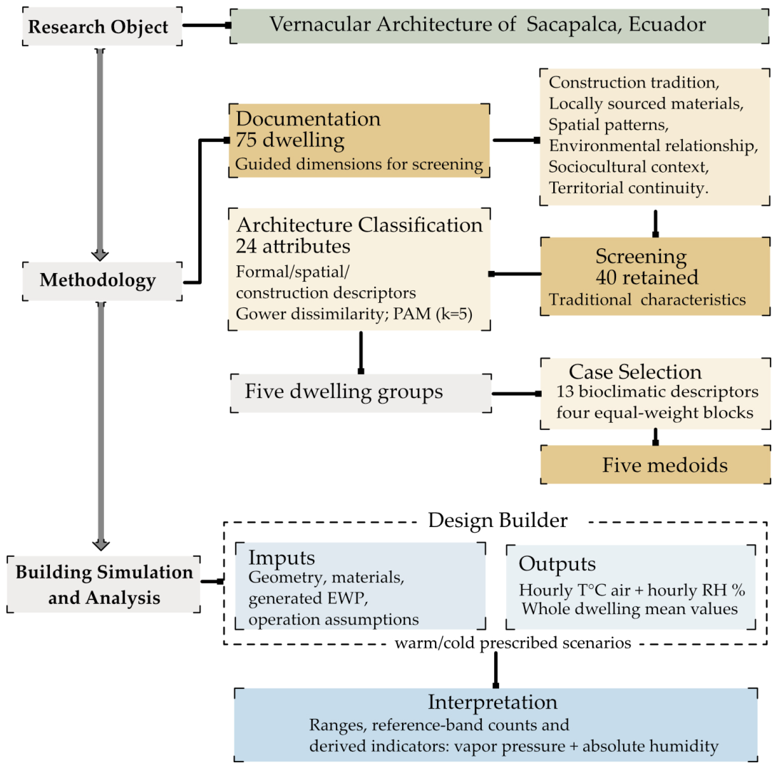
The methodological workflow comprised architectural documentation and screening, classification of the retained dwellings, selection of one medoid per architectural group, simulation of the selected cases, and post-processing of the resulting temperature and relative-humidity outputs. A schematic overview of this sequence is provided in Figure A1.
2.1. Study Area and Location
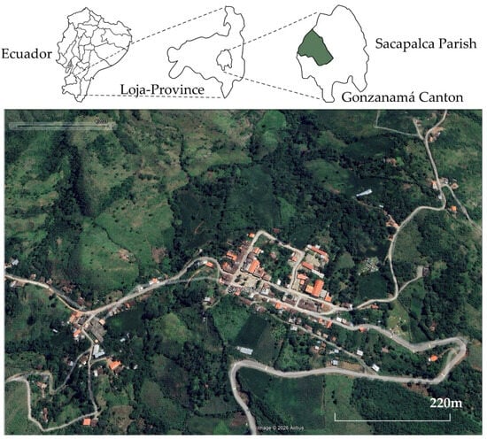
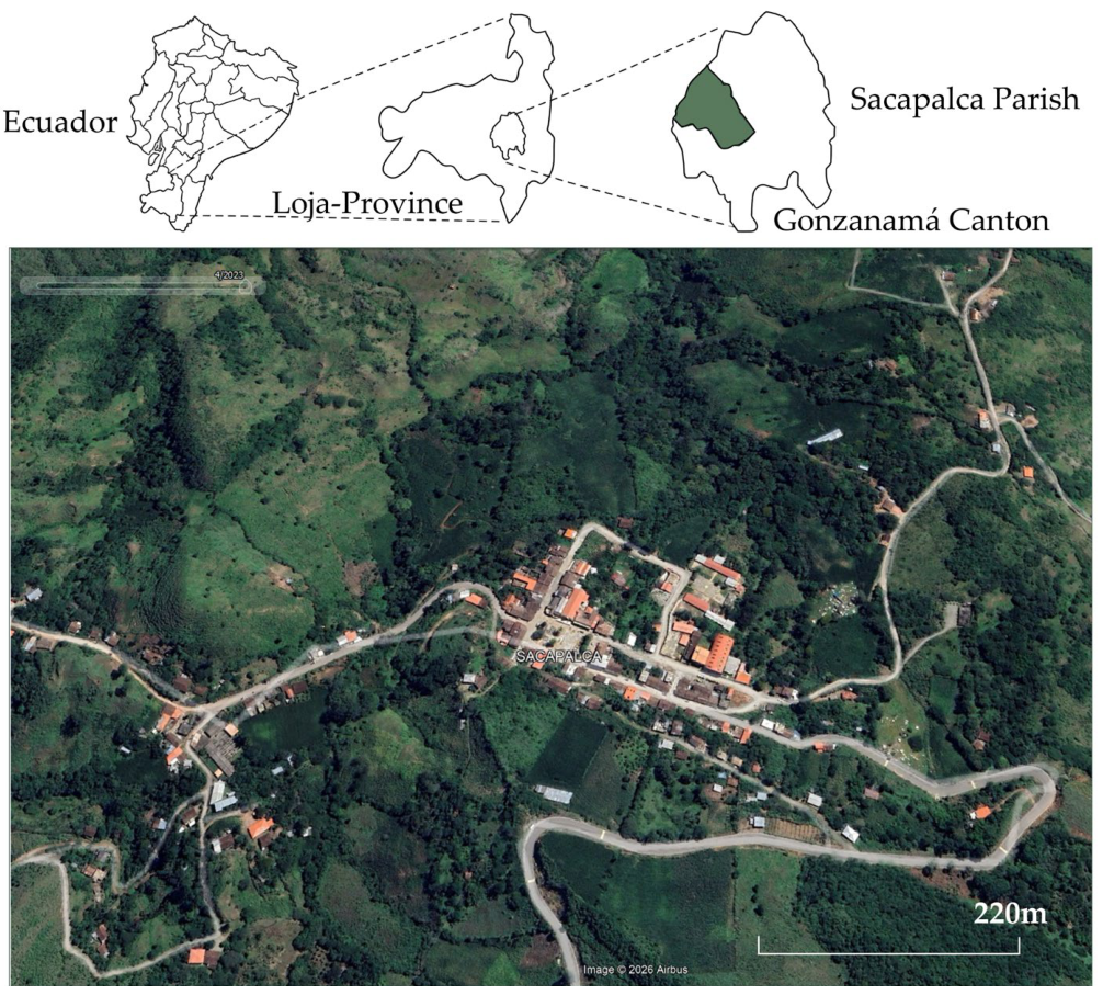
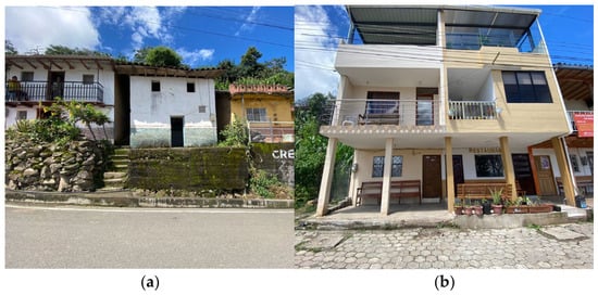
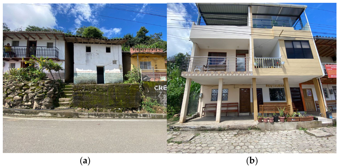
Sacapalca is a rural parish in the Gonzanamá canton, Loja Province, southwestern Ecuador (Figure 1). The parish features a collection of houses built between the 19th and 20th centuries that retain characteristics of Hispanic architecture. Currently, most dwellings in the parish are grouped in the parish seat, where it is possible to find dwellings with vernacular characteristics alongside new constructions that retain some general strategies, such as covered porches and balconies (Figure 2).
Figure 1.
View of the rural parish nestled among mountains, from Google Earth.
Figure 2.
Sacapalca parish, southeastern Ecuador. (a) dwellings with preserved traditional features; (b) an example of contemporary housing typologies.
2.2. Inventory and Case Selection
The field documentation was carried out between April 2023 and April 2024 using survey forms, photographs, and sketches. Architectural documentation was conducted during several site visits using conventional manual measuring tools, survey forms, photographs and sketches to record building geometry and observable architectural and construction characteristics. A matrix of characteristics was established for the selection process based on an inventory of traditional dwellings. Six dimensions were proposed for the initial typological screening to classify the properties:
- •
- Construction tradition (recognized by the community, involving local labor);
- •
- Materiality (use of locally sourced materials);
- •
- Spatial patterns (internal spatial layout, volume, courtyards, roofing, circulation);
- •
- Environmental relationship (orientation, potential for airflow, sun protection and shaded areas, envelope characteristics);
- •
- Sociocultural context (community customs and practices);
- •
- Territorial continuity (similarity to nearby settlements).
These dimensions guided inclusion but do not constitute a numerical score. The inventory reflects the observed state, including substitutions and additions; the study does not reconstruct an unaltered historical condition, given the scarcity of modification records. A total of 75 dwellings were inventoried; contemporary buildings and those with no identifiable relationship to traditional earthen architecture were excluded, leaving 40 cases.
Key spatial similarities among the groups include the absence of an internal courtyard, with corridors or vestibules serving as circulation hubs instead; bay-style layouts featuring one or two street entrances; mixed-use configurations combining residential quarters with one or two commercial areas; and enclosed interior spaces lacking visual permeability. In these spaces, courtyards function as rear setbacks used for secondary purposes, such as bathrooms, storage or vegetable gardens, though not all units feature these rear yards. In two-story dwellings, the upper floor is reserved for private areas, while the ground floor is used for social activities and commercial exchange. Porches connect residents with their surroundings and serve as leisure areas on both levels. Finally, the dwellings consist of a single building volume.
2.3. Architectural Classification and Complementary Checks
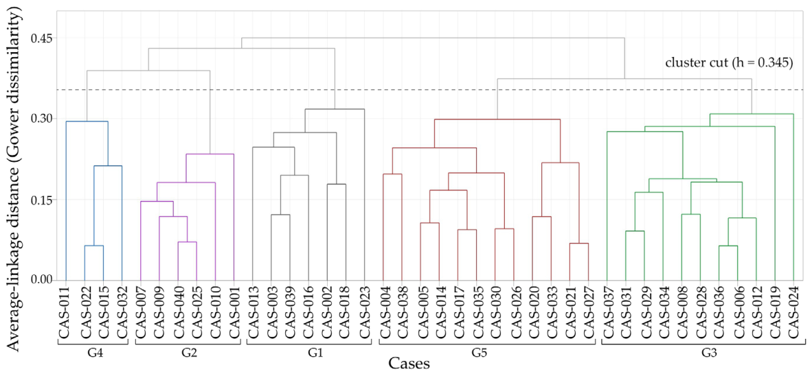
Architectural similarities were examined using Gower dissimilarity [16], which combines quantitative and categorical descriptors, and average-linkage hierarchical clustering. Grouping was based on a five-group partition that constitutes the architectural strata of the study. Its resolution is exploratory, intended to organize patterns at a useful descriptive scale; the inventory does not have a single natural taxonomy. The architectural descriptor specification comprises 24 attributes with equal base weight (Table A1). Quantitative differences are divided by their observed range; nominal variables are compared by matching, and designated ordinal variables use ranked categories. Unobservable or unverifiable values are omitted pairwise, whereas “not applicable” is retained as a category.
A complementary analysis based on partitioning around medoids (PAM) [17] examines a broader representation of 38 attributes, balanced across three blocks: form and spatial organization, construction and finishes, and openings and shading. The mean silhouette [18] describes the separation in this representation, and the adjusted Rand index (ARI) [19] measures the agreement between PAM and average linkage computed on the same stored distance matrix. Stability with respect to attribute selection is examined through 200 subsamples drawn without replacement, retaining 13 of 16, 8 of 10, and 10 of 12 attributes in the respective blocks. Equal weight per block and k = 5 are maintained. This analysis evaluates the dependence on descriptor selection in the complementary specification; it does not redefine the architectural groups or test the thermal models. Complementary clustering results are presented in Table A2 and Table A3.
2.4. Medoid Selection for Bioclimatic Characteristics
Selection was carried out within each architectural group, without modifying group membership. For each pair of dwellings, Gower dissimilarity was computed from 13 descriptors grouped into four blocks (Table 1). Numerical variables were normalized using the ranges of the full inventory of 40 dwellings, and categorical variables were compared by matching.
Table 1.
Descriptors and weights used for medoid selection.
Each block received 25% of the total weight, distributed uniformly among its descriptors. Accordingly, each attribute in a three-descriptor block had a weight of 25%/3 (approximately 8.33%), whereas each attribute in the four-descriptor block received 25%/4 (6.25%). This scheme keeps the nominal influence of each block equal and prevents block weight from depending solely on the number of attributes. The percentages are analytical weights, not physical contributions to thermal behavior.
The medoid was defined as the observed dwelling that minimizes the sum of dissimilarities to the other members of its group, is calculated by Equation (1):
where m_g is group medoid; G_g is the set of dwellings in group g and D_ij is the Gower dissimilarity between dwellings i and j. A check with equal weights for all 13 descriptors identified the same five medoids. Each medoid represents an existing configuration that is central with respect to the attributes considered; its selection does not demonstrate that its thermal response is typical of all members of the group.
m_g = arg min_(i∈G_g) Σ_(j∈G_g) D_ij,
2.5. Meteorological Reference and Daily Scenarios
Owing to the scarcity of historical climate records for the study locality, a reference EPW (EnergyPlus Weather File) was generated with Meteonorm v8.1 [20]. This dataset was defined at a latitude of −4.155°, longitude of −79.518°, altitude of 1530 m, and time zone UTC−5, and contains 8760 hourly records. For this generated record, the mean annual dry-bulb temperature is 17.88 °C, and monthly means range from 15.43 °C to 20.77 °C.
Two 24-record scenarios are examined: 6 January, designated as warm, and 14 June, designated as cold. Outdoor temperatures on these dates span 14.4 °C to 24.8 °C and 13.4 °C to 19.5 °C, respectively. The analysis uses indoor extremes, daily amplitudes, and counts relative to the reference intervals, without calculating instantaneous indoor-outdoor differences, time lag, or decrement factors. No independent, complete local historical weather series was available to evaluate bias.
2.6. Models and Operational Assumptions
The dwellings were represented in DesignBuilder v6 [21] from the surveyed geometry and orientation. Rooms were represented as thermal zones, and air temperature and relative humidity were expressed as whole-dwelling averages. This is because the groupings were based on construction or technological characteristics, combined with the high variability of internal layouts among dwellings (owing to users’ individual adaptations and modifications). The simulations therefore do not reconstruct the contributions of each zone, and the unit of analysis is the aggregate response of the building. Heating and mechanical cooling (neither of which was found in any dwelling) were excluded, and plug-in equipment loads were discarded. Terrain and vegetation were not considered in the simulation. Two of the five simulated dwellings (CASE 5 and CASE1) are partially attached to neighboring buildings in the actual settlement, an influence that the models do not represent. Mutual shading and wind sheltering were therefore not assessed, and the results describe each configuration in isolation and not the settlement environment. The party walls were modeled as exposed exterior walls.
The common reference wall section comprises (from inside to outside) 13 mm of plaster, 30 mm of earthen render, 340 mm of adobe, 30 mm of render, and 13 mm of plaster, for a total thickness of 426 mm. The assigned thermal conductivities were 0.57, 0.40, 0.22, 0.40, and 0.57 W m−1 K−1. Properties for most materials were taken from the software library, whereas those for adobe were obtained from a study in a nearby area [22] and were not measured locally. Table A4 summarizes the properties used for the walls.
Roofs and floors were represented using common templates from the program library. The roof includes clay tiles and an air cavity. For cases with windows, these were assigned to categories of single glazing, timber or metal frames, and solid timber doors. These decisions constitute a simplified representation of the observed buildings, without reconstructing each material substitution. The optical properties and the permeability classes of joinery, which would be needed to attribute their effects quantitatively, were not considered.
Hygroscopic moisture storage in earthen walls was not modeled. Its effect on the simulated daily relative humidity amplitudes was therefore not quantified, and neither the direction nor the magnitude of any resulting bias has been established.
Natural ventilation was prescribed using the Scheduled option. In the warm scenario, the nominal rate is 12 air changes per hour (ACH), an average value that considers full opening of the openings during the warm season and was set from direct field observation of how occupants use them. This rate is multiplied by the Dwell_DomCommonAreas_Occ schedule, in addition to a continuous infiltration of 0.7 ACH. In the cold scenario, only the 0.7 ACH infiltration is applied. The ventilation coefficients for the constant, temperature, velocity, and velocity-squared terms are 1, 0, 0, and 0. The schedule thus modulates a prescribed rate, without deriving the airflow from the geometry of the openings or from wind pressure. Transoms are retained as architectural descriptors; no independent airflow contribution is calculated for them. Information on the operating assumptions and documented ventilation controls is summarized in Table A7.
Occupancy density was 0.043 people m−2, with common assumptions for activity and occupancy, a metabolic factor of 0.90, and nominal clothing values of 1.0 and 0.50 clo. Lighting was specified as 5 W m−2 per 100 lux; without the corresponding illuminance, it cannot be converted into a verified effective load. Equal densities and operating rules do not imply equal total internal gains in buildings of different size.
The models were neither empirically calibrated nor validated, and adobe conductivity, infiltration, and ventilation rates were not measured locally. No thermal-parameter sensitivity or uncertainty-propagation analysis was performed. The reported values therefore describe the models under the prescribed inputs and support exploratory comparisons conditional on those assumptions. Common weather data and operating rules do not ensure that input uncertainties affect all cases equally. The magnitude and ordering of differences between cases may change under alternative parameter values; their robustness remains untested.
Within these limits, the study links the architectural documentation and classification of the surveyed dwellings to an explicit procedure for selecting individual cases for simulation. Medoid selection provides a reproducible basis for choosing configurations that are central in the selected descriptor space, although it does not establish their thermal representativeness. The simulations complement this characterization by examining the responses of five selected configurations under documented scenarios. They provide a basis for formulating hypotheses and identifying comparisons for subsequent investigation, while their correspondence with actual indoor conditions and their generalizability to other dwellings remain to be evaluated.
2.7. Environmental Indicators and Interpretation
The adaptive relationship of ASHRAE 55 [23], Tc = 0.31 Tpma + 17.8 °C, was used with an interval of ±3.5 °C. The prevailing mean outdoor temperature (Tpma) was computed as the mean of the daily mean outdoor temperatures of the 30 days preceding the analyzed day, using the generated weather file. Tpma = (1/30) × Σ T_ext,d, for d = 1 to 30. Each daily mean was calculated from the 24-hourly outdoor temperature records, and the analyzed day was not included in the average. For the warm scenario (6 January), the period used was 7 December to 5 January, giving Tpma = 18.83 °C. For the cold scenario (14 June), it was 15 May to 13 June, giving Tpma = 17.66 °C. Tpma values are reported rounded to two decimals; all subsequent calculations were performed with unrounded values. The weather file represents a typical year and not a continuous series, so it was treated as cyclic for January, with December taken from the same file. Applying the adaptive relationship with limits of Tc ± 3.5 °C yields 20.14–27.14 °C for 6 January and 19.78–26.78 °C for 14 June. Because the weather series is generated and not measured, these intervals inherit its uncertainty and are used as an indicative reference, not as a classification criterion. They provide context for the outputs: the adaptive method refers to operative temperature and has specific conditions of applicability, whereas aggregated air temperature is used here. No extension for elevated air speed was applied.
For each case and scenario, the minimum, maximum, and daily amplitude of the 24 air temperature records were calculated, together with counts below, within, and above the thermal reference. Relative humidity was summarized using a descriptive interval of 40–60%, selected for this analysis and not considered a mandatory ASHRAE 55 criterion or a health threshold. The counts correspond to hourly records, without interpolation or occupancy weighting. No inferential significance tests were applied, since the outputs are serial deterministic results from individual models and not independent experimental replicates.
To examine whether relative humidity variations could be explained by temperature alone, vapor pressure and absolute humidity were derived from paired hourly whole-dwelling mean temperature and relative humidity using a Buck-type saturation pressure expression [24]. These nonlinear transformations of aggregated values may differ from averages of zone-level indicators; the aggregation effect remains unquantified. The derived indicators help distinguish temperature-related changes in relative humidity from changes in vapor content, but reported percentage differences remain diagnostic and cannot quantify moisture sources, ventilation removal, or hygroscopic exchange with adobe, which was not modeled.
3. Results
3.1. Group Structure and Architectural Patterns
The five groups contain 7, 6, 11, 4, and 12 dwellings, respectively. Thirty-nine records describe adobe walls with a width of approximately 0.40 m; only one case (CAS-024), in group 3, has a 0.35 m bahareque wall. CAS-024 is not the medoid of its group and is therefore not among the five modeled dwellings, so the common adobe section does not misrepresent any simulated case. The inventory thicknesses describe the surveyed construction and are distinct from the layered section that characterizes the materials in the model. Timber roof structures and clay tile recur, together with substituted finishes and joinery. Common construction therefore coexists with differences in layout and facade articulation.
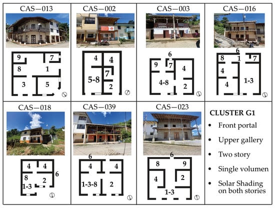
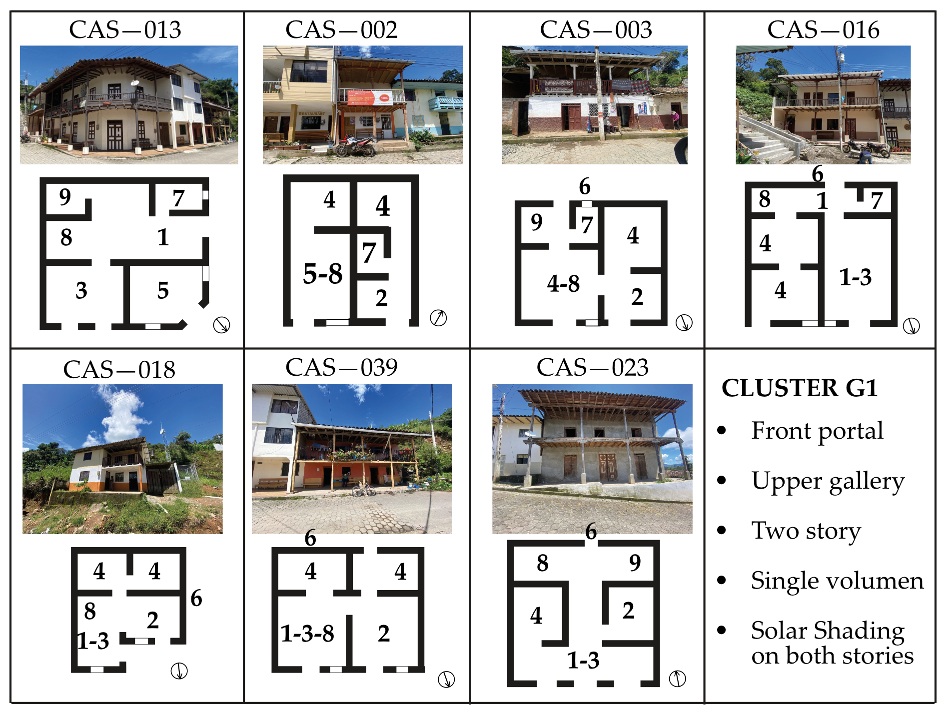
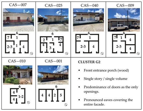
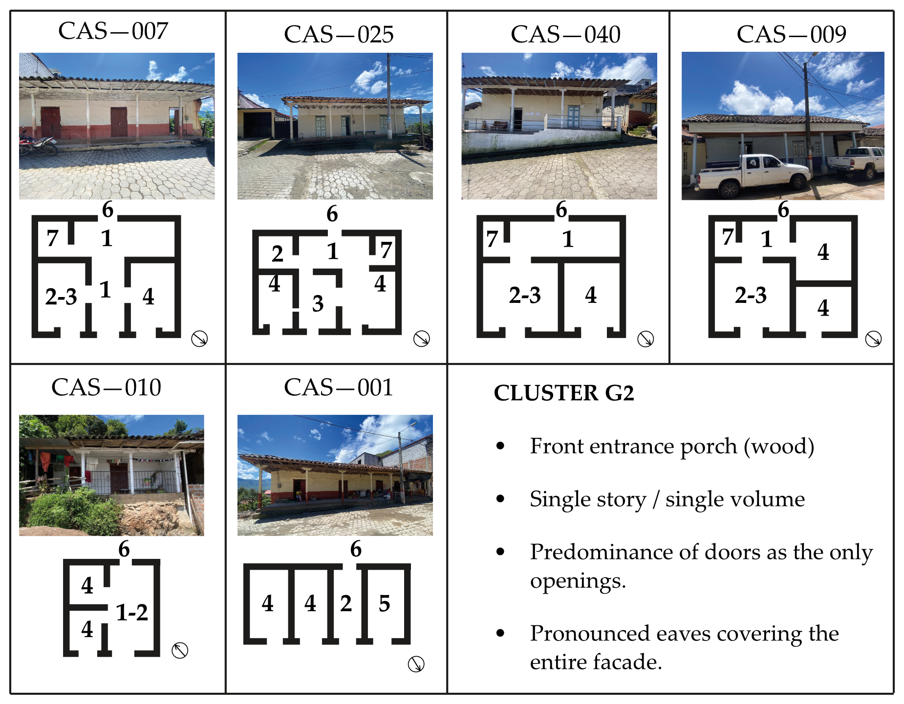
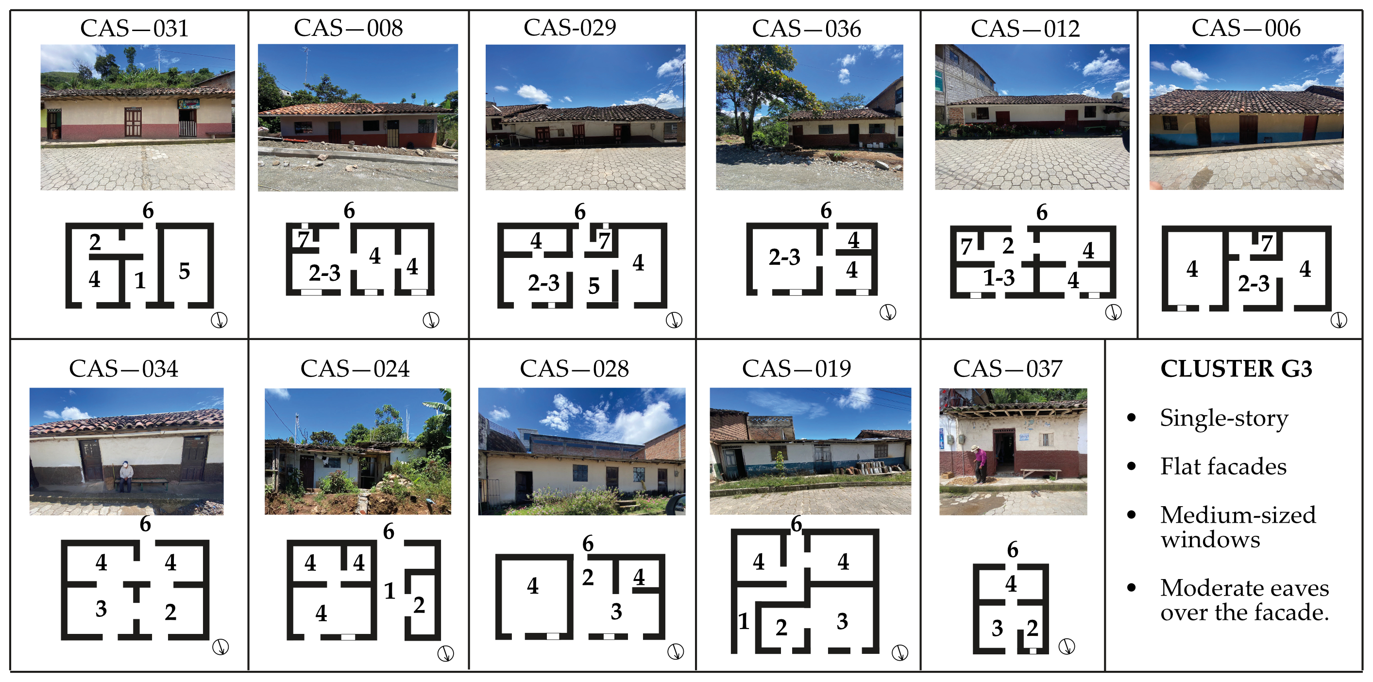
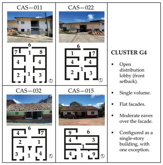
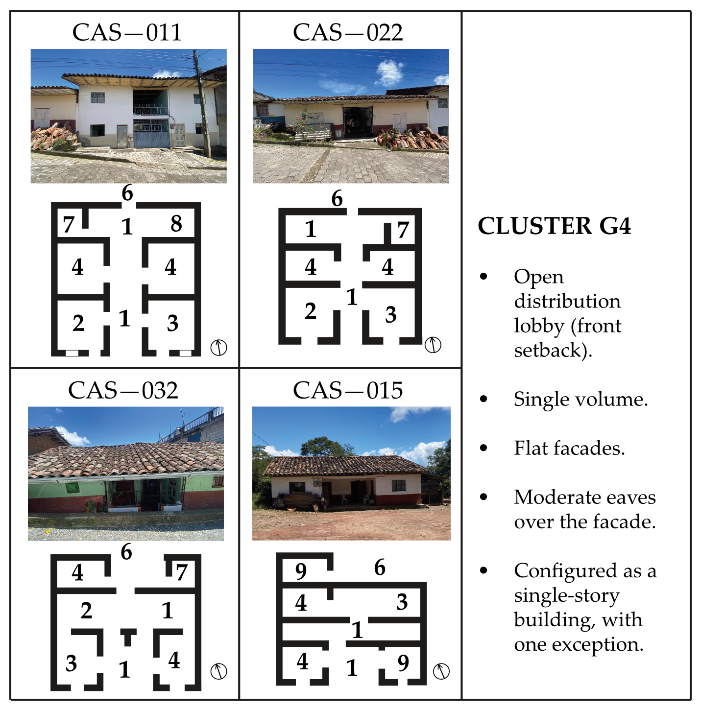
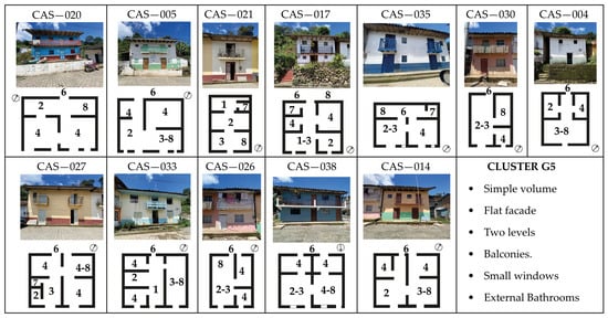
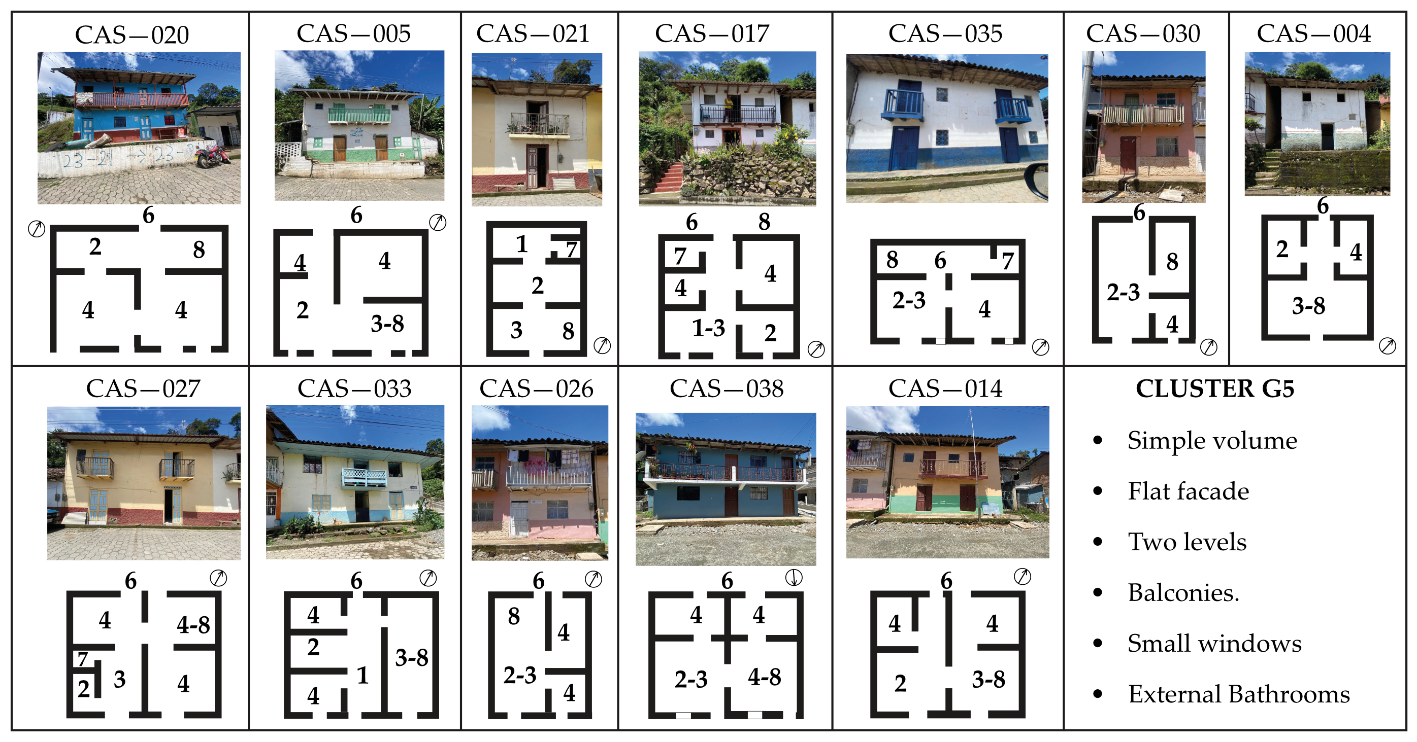
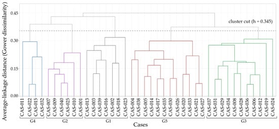
G1 and G5 comprise two-story configurations. Protection by means of covered porches characterizes G1, including the upper exterior portal of CAS-003; G5 combines eaves with upper galleries or balconies. G2 brings together single-story dwellings with protection associated with porches, whereas G3 contains single-story configurations with eaves. G4 includes three single-story dwellings and one two-story dwelling, with set-back entrances and eaves. These descriptions identify recurring combinations, without attributing each membership to a single characteristic. Figure 3, Figure 4, Figure 5, Figure 6 and Figure 7 show buildings and spatial diagrams; spatial diagrams are presented instead of scaled floor plans to protect the privacy of the occupants; the dimensional data used in the analysis are reported in Table 2; Figure 8 presents the architectural dendrogram.
Figure 3.
Cluster G1: View of the cases in their current condition. The diagrams are not metric-scale plans. Key: 1 hall/corridor; 2 kitchen/dining; 3 living room; 4 bedroom; 5 commercial space; 6 garden; 7 sanitary facility; 8 vertical circulation; 9 storage. White gaps indicate openings; arrows indicate orientation.
Figure 4.
Cluster G2: View of the cases in their current condition. The diagrams are not metric-scale plans. Key: 1 hall/corridor; 2 kitchen/dining; 3 living room; 4 bedroom; 5 commercial space; 6 garden; 7 sanitary facility; 8 storage. White gaps indicate openings; arrows indicate orientation.
Figure 5.
Cluster G3: View of the cases in their current condition. The diagrams are not metric-scale plans. Key: 1 hall/corridor; 2 kitchen/dining; 3 living room; 4 bedroom; 5 commercial space; 6 garden; 7 sanitary facility. White gaps indicate openings; arrows indicate orientation.
Figure 6.
Cluster G4: View of the cases in their current condition. The diagrams are not metric-scale plans. Key: 1 hall/corridor; 2 kitchen/dining; 3 living room; 4 bedroom; 5 commercial space; 6 garden; 7 sanitary facility; 8 vertical circulation; 9 storage. White gaps indicate openings; arrows indicate orientation.
Figure 7.
Cluster G5: View of the cases in their current condition. The diagrams are not metric-scale plans. Key: 1 hall/corridor; 2 kitchen/dining; 3 living room; 4 bedroom; 5 commercial space; 6 garden; 7 sanitary facility; 8 vertical circulation. White gaps indicate openings; arrows indicate orientation.
Table 2.
Geometry and attributes of the five selected cases. S/V: envelope surface area per unit of interior volume; OWR: door and window area relative to exposed façades containing openings.
Figure 8.
Architectural dendrogram of the inventory. The branches represent the archived hierarchical analysis; G1–G5 correspond to the groups defined in the study.
For the stored complementary Gower matrix, PAM with k = 5 produced a mean silhouette of 0.372 and an ARI of 0.915 with respect to average linkage. The matrix reconstructed from the 38 attributes produced a mean silhouette of 0.368. Its PAM partition with k = 5 coincided with that obtained by PAM on the stored Gower matrix (ARI = 1.000). This agreement refers to the two PAM partitions and not to their comparison with the adopted architectural groups. Across 200 attribute subsamples, the ARI with respect to the full PAM had a mean of 0.858, a median of 0.915, and a 10th–90th percentile range of 0.670–1.000. The median coincides numerically with the ARI between methods (0.915), but the two values come from different comparisons (PAM versus average linkage, and subsampled PAM versus full PAM), and different partitions can yield the same ARI. These values describe agreement within the complementary analysis. The moderate silhouette and the variation among subsamples are compatible with an exploratory classification whose boundaries depend partly on the descriptors.
3.2. Selected Cases and Bioclimatic Variation
The selected medoids are CAS-003, CAS-025, CAS-031, CAS-015, and CAS-030, hereafter referred to as CASES 1–5. Table 2 presents their geometry and opening-related attributes. CASE 1 combines two stories, an attached configuration, and a portal. CASE 2 is a detached single-story dwelling with an over-door transom; CASE 3 is a single-story attached dwelling with eaves. CASE 4 is a single-story detached dwelling with a recessed entrance and no recorded transom. CASE 5 combines two stories, an attached configuration, eaves, and an upper gallery. Each selection preserves the architectural identity of its group while identifying, within that group, an observed combination of bioclimatic descriptors.
OWR ranges from 2.98% in CASE 5 to 8.92% in CASE 3. CASE 2 has an OWR of 3.33% and CASE 4 an OWR of 7.06%, with surface-to-volume ratios of 0.819 and 0.735 m−1, respectively. Table A5 and Table A6 report group medians and ranges to contextualize the selection. The medoid is not required to coincide with the median of any individual descriptor, because its selection minimizes dissimilarities across the four analytical blocks—nor does its selection imply that other members of the group would reproduce the same simulated trajectory. Differences between the five simulated cases should therefore not be interpreted as a typology-level performance ranking, since within-group variability in thermal responses remains unquantified.
3.3. Air Temperature Under the Warm Scenario
All temperatures, daily amplitudes, and threshold counts reported in the following Sections are simulated outputs conditional on the prescribed inputs. They support exploratory comparisons between the modeled configurations, rather than validated estimates of actual indoor conditions. Counts indicate hourly whole-dwelling mean air temperatures relative to the indicative reference interval and should not be interpreted as observed discomfort hours or evidence of ASHRAE 55 compliance.
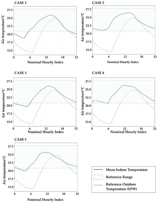
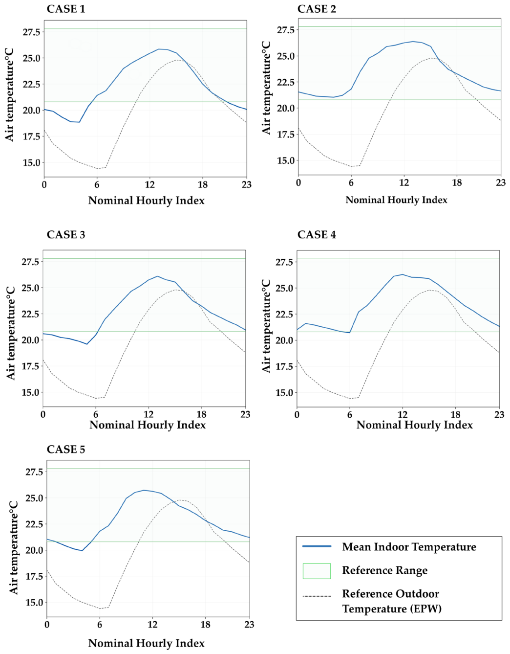
The simulated air temperature in CASE 1 ranged from 18.85 °C to 25.85 °C, with a daily amplitude of 7.00 °C; six of the 24 hourly records were below the lower reference threshold of 20.14 °C. CASE 2 ranged from 21.05 to 26.38 °C, with a daily amplitude of 5.33 °C, and all records remained within the reference interval. CASE 3 ranged from 19.60 °C to 26.10 °C, with three records below the lower threshold. CASE 4 ranged from 20.72 °C to 26.30 °C, with all records within the interval. CASE 5 ranged from 19.94 °C to 25.73 °C, with two records below the lower threshold. None of the cases exceeded the upper reference threshold of 27.14 °C (Figure 9).
Figure 9.
Whole-dwelling mean air temperature for each dwelling in the warm scenario of 6 January. Dashed line: EPW (EnergyPlus Weather File) outdoor dry-bulb temperature; shaded band: indicative thermal interval.
For each model, the series describes the daily temperature evolution under scheduled ventilation and assigned internal gains. The absence of values above the upper reference threshold is a characteristic of these simulated air-temperature outputs. It does not quantify the specific effect of the 12 ACH ventilation rate, because the rate was schedule-dependent and no alternative ventilation scenario was simulated for the same day. Likewise, the small differences among peak temperatures do not establish a practically meaningful performance advantage.
3.4. Air Temperature Under the Cold Scenario
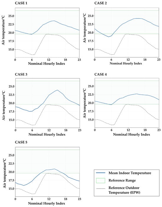
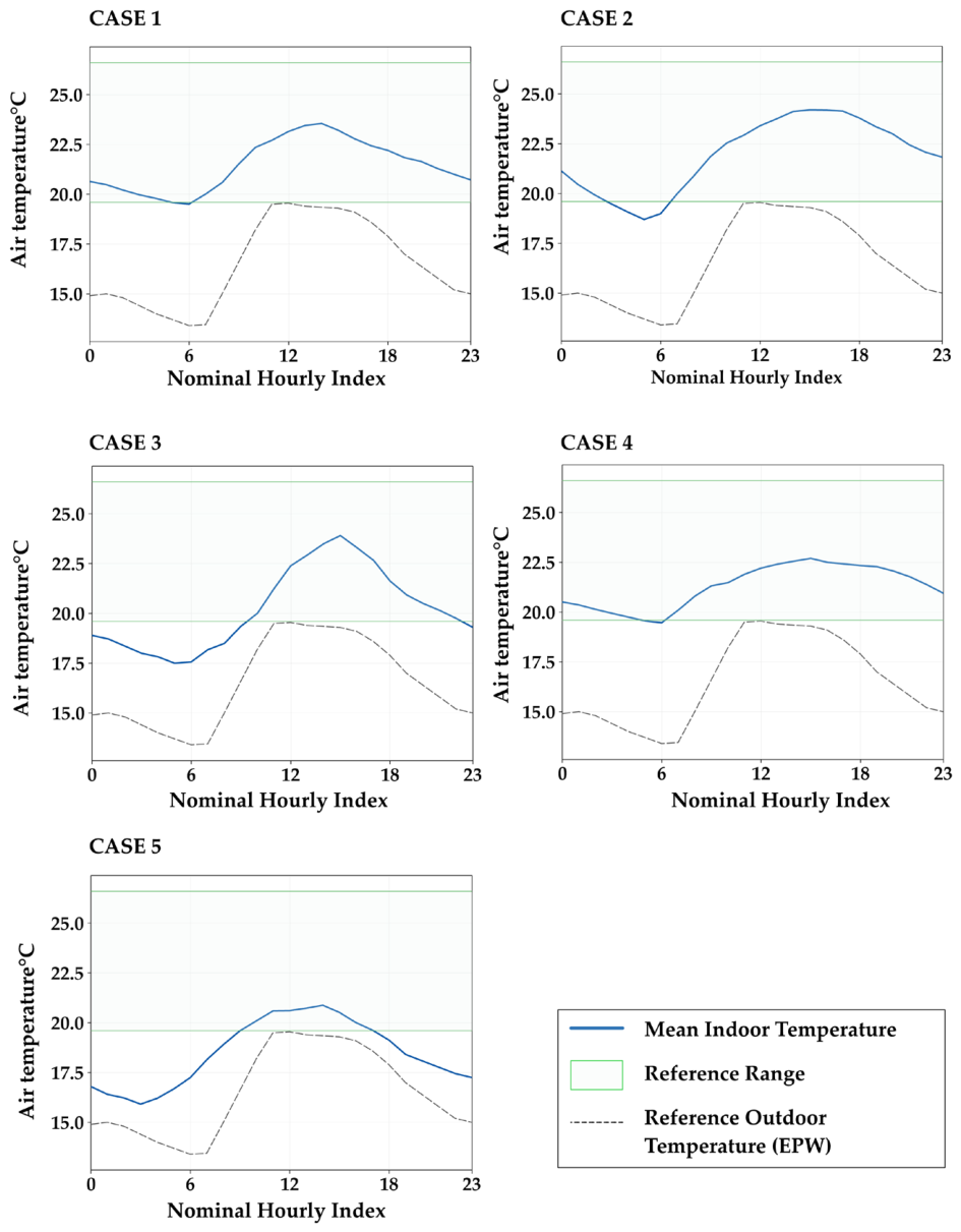
For the cold scenario, simulated air temperature in CASE 1 ranged from 19.51 °C to 23.55 °C, with a daily amplitude of 4.04 °C and two hourly records below the lower reference threshold of 19.78 °C. CASE 2 ranged from 18.70 °C to 24.20 °C, with four records below the threshold. CASE 3 ranged from 17.50 °C to 23.91 °C, with a daily amplitude of 6.41 °C and 12 records below the threshold. CASE 4 ranged from 19.47 °C to 22.70 °C, with a daily amplitude of 3.23 °C and three records below the threshold. CASE 5 ranged from 15.92 °C to 20.88 °C, with 17 records below the threshold. None of the cases exceeded the upper reference threshold of 26.78 °C (Figure 10).
Figure 10.
Average Air Temperature of Each Dwelling under the Cold Scenario on 14 June. Dashed line: EPW (EnergyPlus Weather File) outdoor dry-bulb temperature; shaded band: indicative thermal interval.
The cold-scenario series shows lower-threshold deviations in all selected cases, although their duration differs over the reported day. CASE 4 therefore does not remain within the reference interval for all hourly records, while CASE 5 reaches the lowest temperatures under a scenario in which infiltration was the only prescribed air-exchange mechanism. Its gallery, orientation, and opening ratio describe the architectural configuration associated with this response, but the simulations do not isolate the contribution of each factor. The reported daily amplitudes characterize whole-dwelling air temperature and should not be interpreted as direct measures of the dynamic thermal properties of the walls or roof.
3.5. Relative Humidity and Derived Vapor Indicators
In the warm scenario, CASES 1 and 5 remain within the descriptive relative humidity interval of 40–60% for all 24 records. CASE 2 reaches 69.64% and has seven records above 60%. CASE 3 has one record below 40%, at 39.95%, and CASE 4 has two, with a minimum of 39.18%. These small lower deviations describe numerical positions relative to the chosen interval; the CASE 3 value does not establish a relevant change in environmental acceptability.
In the cold scenario, CASES 1, 3, 4, and 5 have 10, 8, 12, and 6 records above 60%, respectively. CASE 2 has five records below 40% and none above 60%. Its range of 36.69–52.15% shows that the lower-temperature scenario does not imply higher relative humidity in all cases or records. These are whole-dwelling averages; the results do not locate damp surfaces or identify moisture problems by room. Table 3 summarize the warm and cold response.
Table 3.
Relative humidity and counts relative to the descriptive 40–60% range. Counts correspond to 24 records per series and do not represent occupant exposure.
The derived absolute humidity spans 8.33–12.01, 10.14–14.08, 8.17–12.28, 9.33–11.52, and 8.10–11.02 g m−3 for CASES 1–5 in the warm scenario. The respective cold ranges are 9.31–12.68, 8.04–10.15, 8.27–12.48, 9.22–12.73, and 7.38–10.00 g m−3. Vapor pressure also varies (Table A8). These percentages describe changes in vapor pressure and absolute humidity calculated from whole-dwelling mean temperature and relative humidity. Part of this variation may arise from averaging these variables before applying the nonlinear psychrometric equations. The percentages should therefore be treated as diagnostic observations of the aggregated outputs, rather than as quantitative attribution to specific moisture-balance mechanisms.
4. Discussion
The analysis shows that architectural typology and thermal representativeness are not equivalent. A group can be architecturally coherent and still have meaningful differences in terms of compactness, openings, shading, ventilation potential and envelope configuration.
4.1. Architectural Classification and Environmental Interpretations
The classification describes the recurrence of formal and functional decisions in a heterogeneous earthen inventory. The repetition of porches, eaves, vestibules, and upper galleries is of architectural interest even when their thermal contribution is not quantified. These spaces organize circulation, street access, and uses protected from the sun; walls and openings define the enclosure. Describing them together provides a basis for heritage assessment that would be lost by reducing the inventory to a wall material or a facade proportion.
The intragroup medoid analysis adds an explicit selection rule to this description. It preserves the five strata and considers the internal geometric and environmental variation. The medoid represents the central combination of the selected inputs, without defining an ideal building or the response of the whole group.
Only one dwelling per group was simulated, in line with the exploratory aim of characterizing existing configurations selected by an explicit, reproducible rule, not of estimating the distribution of thermal behavior within each group. All dissimilarities reported here were computed with the 13-descriptor Gower matrix used to select the medoids, and not with the 24-attribute matrix used to form the groups. The mean dissimilarity between each medoid and the other members of its group was 0.131 (G1), 0.078 (G2), 0.108 (G3), 0.130 (G4), and 0.130 (G5). The mean over all pairs within a group was higher (0.163; 0.111–0.188 by group), because the medoid is by definition the member closest to the rest. It was in turn lower than the mean between dwellings of different groups (0.369; 0.326 across all 780 pairs). Separation between groups was not uniform: G2 and G3 were the closest pair (0.243), followed by G1 and G5 (0.289), although both values exceed the within-group means of the groups involved. The inventory shares a common constructive base, so within-group differences concern mainly layout, facade articulation, and openings. These differences may alter the response of non-simulated members, and the intragroup variability of the thermal trajectories therefore remains unquantified. The series are interpreted as case studies linked to a classification, and no thermal label is assigned to the 40 dwellings. Future work can quantify within-group variability by simulating additional dwellings that span the descriptor ranges of each group, including those most dissimilar to the medoid. Under common weather and operating assumptions, comparing their temperature trajectories, daily amplitudes, and hourly records relative to the reference interval would show how much each group disperses and where groups overlap. A sensitivity analysis on the input values would then test whether those patterns hold.
4.2. Interpretation of Overall Responses
At the building scale, the evolution of air temperature depends on heat transfer and storage in the envelope, solar and internal gains, and air exchange, and geometry and exposed surface condition how these terms act. The daily amplitudes reported here summarize the joint response of the prescribed model and do not isolate any of these terms. Wall thickness, opening proportion, and shading are therefore treated as descriptors of each configuration, and the results are not used to attribute thermal effects to individual features.
The same restraint applies to transoms and to other operable openings. Their position may allow air exchange near the entrance, but the scheduled ventilation does not compute their airflow separately, and a whole-dwelling average can dilute a local effect. Their ventilation potential is recognized as an architectural characteristic, without quantifying benefits. Likewise, shading and openings may serve competing functions, such as reducing solar gains in warm weather while limiting useful gains in cold weather. Quantifying them would require controlled variants of the same building under the same weather, which is beyond the scope of this exploratory study. The scenarios do not support conclusions on retrofit or optimization.
The relative vapor pressure ranges reported in Table A8 indicate that the derived indicator fluctuated over the day in every case and scenario. These results describe the relative daily variation in the derived indicator and complement the relative humidity analysis. A larger percentage denotes a greater range relative to the series minimum, but does not necessarily indicate a larger absolute range or higher vapor pressure. Comparisons between cases therefore require considering these percentages alongside the corresponding vapor pressure values.
4.3. Relationship with Regional and Simulation Studies
The Azogues study [2] provides a regional example of the analysis of spatial organization and passive strategies; the Andean study by Miño-Rodríguez et al. [11] shows the additional evidence that monitoring and calibration provide. The coastal bamboo study [3] corresponds to a different envelope system and climate. These precedents justify attention to configuration and to methodological scope, without providing equivalent controls for Sacapalca. No measured or simulated alternative with contemporary materials was included, so advantages over concrete block or other substitute systems cannot be quantified.
Simulation research, such as the examination of thermal inertia in vernacular architecture by Montalbán Pozas and Serrano [25], allows specific configurations to be formulated and examined. Its evidentiary strength depends, however, on the inputs implemented and on the validation design. Program evaluation through frameworks such as ASHRAE Standard 140 [26] refers to the behavior of the simulation engines and does not validate the model of a specific dwelling. In Sacapalca, the contribution lies in connecting architectural documentation, explicit selection, and conditioned global response, with empirical evaluation still pending.
4.4. Limitations and Scope of Inference
This study is exploratory and comparative. It links an architectural inventory with a numerical characterization of existing configurations under prescribed scenarios, so its outputs are read as relative responses and not as absolute assessments of the actual dwellings. Within this framework, the models were not empirically calibrated or validated. The remote location of Sacapalca constrained field monitoring, while the limited availability of historical climate records restricted the local climatic information available for the study. Continuous, concurrent indoor and outdoor temperature and humidity measurements were not collected. Material properties and infiltration were assigned as prescribed assumptions, without local measurements of conductivity, wall moisture, or airtightness. Internal partitions and floors were included in the models, but their thermal capacity was not characterized in detail, and furniture was not modeled. Results are reported as the arithmetic mean of the room-level values of each dwelling, so small and large rooms contribute equally, and the aggregate may differ from a volume-weighted value. Simulated daily amplitudes are therefore interpreted as aggregate model responses, not as measures of thermal inertia.
The two daily scenarios are illustrative and do not represent annual performance. They differ in their meteorological and ventilation conditions, so the influence of each is not separated. The outdoor series from the EPW file is contextual, and no time lag or instantaneous indoor-outdoor effects are therefore inferred. Whole-dwelling mean air temperatures omit radiant conditions, local air speed, room-level variability, and the actual adaptive behavior of occupants, aspects that require measurements and a different study design. No uncertainty propagation or sensitivity analysis of thermal parameters was carried out. The common operating rules reduce input differences among cases, although they do not guarantee that errors cancel out. The 24-attribute clustering and the complementary 38-attribute PAM analysis serve different functions: the former defines the architectural groups, and the latter examines their dependence on descriptor selection.
These decisions delimit the available evidence without invalidating the descriptive inventory or the value of the results for formulating hypotheses. Among them are the role of porches and eaves in the configuration of each group and the possible hygroscopic buffering by adobe. Because each simulated case shares material and formal characteristics with other dwellings in its group, the results provide a basis for formulating hypotheses about how these characteristics may relate to thermal response, informing future research on design and rehabilitation. Evaluating these hypotheses requires comparing simulation outputs with on-site measurements. Extending the findings to other dwellings within the architectural groups would also require assessing within-group thermal variability and the sensitivity of the results to uncertain input parameters, following the approach proposed in Section 4.1. Within this scope, the results help define research questions and priorities for future monitoring campaigns, without constituting design prescriptions.
5. Conclusions
The study documents a rural parish in the southern Andes where earthen construction persists, a context that is underrepresented in the Ecuadorian literature on the environmental performance of vernacular architecture. Of 75 inventoried dwellings, 40 retained traditional characteristics and were organized into five groups using Gower dissimilarity and average linkage. The groups are distinguished by recurring combinations of number of floors, protection by porches or eaves, and upper galleries or balconies, on a common constructive base of adobe walls approximately 0.40 m thick, timber roof structures, and clay tile. This joint description provides a basis for heritage assessment that would be lost by reducing the inventory to a wall material or a facade proportion.
The selection procedure is a reproducible contribution. An independent analysis of 13 descriptors, organized into four blocks of equal weight, identified one observed dwelling per group without altering the architectural classification. The medoids were at a mean dissimilarity of 0.08 to 0.13 from the other members of their group, compared with 0.37 between dwellings of different groups, and a check with equal weights for the 13 descriptors identified the same five medoids. For these cases, exploratory simulations characterized whole-dwelling air temperature and relative humidity under two prescribed daily scenarios.
In these simulated scenarios, indoor temperature amplitudes were 5.33 °C to 7.00 °C in the warm scenario and 3.23 °C to 6.41 °C in the cold scenario. No record exceeded the indicative upper thermal reference in either scenario, and in the cold scenario all cases had records below the lower limit. Derived vapor-pressure and absolute-humidity indicators varied across the aggregate series. These diagnostic transformations are affected by spatial aggregation and do not establish the mechanisms responsible for moisture variation.
Given their exploratory and comparative nature, these results describe the relative responses of five existing configurations. They do not establish hierarchies among groups or attribute effects to porches, eaves, openings, or hygroscopic buffering by adobe, which remain hypotheses. Nor do they generalize to the other members of each group, of which only one was simulated. The findings apply to the five simulated cases under the prescribed assumptions. Continuous on-site monitoring with concurrent weather data would test them against measured behavior. Annual simulations, sensitivity analyses, and dwellings more distant from the medoid would extend them to the architectural groups, and controlled variants of a single building would isolate the effect of each element.
Author Contributions
Conceptualization, E.A.-M. and E.C.; methodology, E.A.-M.; software, E.A.-M. and E.C.; validation, C.B.-A., E.A.-M. and E.C. (internal review of the modeling workflow and outputs; not empirical validation against field measurements); formal analysis, E.A.-M. and E.C.; investigation, E.A.-M. and E.C.; resources, E.A.-M. and E.C.; data curation, C.B.-A. and E.C.; writing—original draft preparation, E.A.-M.; writing—review and editing, E.A.-M. and C.B.-A.; visualization, E.A.-M. and E.C.; supervision, E.A.-M.; project administration, E.A.-M. All authors have read and agreed to the published version of the manuscript.
Funding
This research received no external funding.
Data Availability Statement
Data presented in this study are available from the corresponding author upon reasonable request.
Acknowledgments
During the preparation of this manuscript, the author(s) used GPT-5.6 Luna for language editing, including grammar, spelling, and phrasing. All AI-assisted outputs were reviewed and verified by the authors and take full responsibility for the content of this publication.
Conflicts of Interest
The authors declare no conflicts of interest.
Abbreviations
The following abbreviations are used in this manuscript:
| ACH | Air Changes per Hour |
| ARI | Adjusted Rand Index |
| EPW | EnergyPlus Weather File |
| OWR | Opening-to-Wall Ratio |
| PAM | Partitioning Around Medoids |
| RH | Relative Humidity |
| S/V | Surface-to-Volume Ratio |
| AH | Absolute Humidity |
Appendix A
Appendix A.1
Figure A1.
Sequence of the analysis.
The architectural analysis uses mixed descriptors of spatial organization, construction and façade elements. The 24-attribute specification has equal base weights of 1. For complete pairs each attribute therefore contributes 1/24 of the distance denominator; missing pairs change the effective relative weights. The dictionary below specifies the computational representation rather than inferring variable types from their names.
Table A1.
Architectural descriptor specification. All 24 base weights equal 1. The original field front_portal denotes recessed_entrance.
Appendix A.2
PAM [S2] at k = 5 was computed on the saved full-data Gower matrix using deterministic BUILD and SWAP. Average linkage was computed from that same matrix for the cross-method comparison. A raw-feature reconstruction uses 38 attributes with equal block contributions of 1/3 and equal variable weights within each block. These 38 attributes define a separate complementary specification, not a replication of the 24-descriptor dendrogram. Direct access count is ordinal; window opening size uses nominal matching in this complementary specification.
Table A2.
Retained attributes in the complementary PAM specification.
The case identifier, an entirely missing eave-location descriptor, invariant attributes and the redundant upper-timber-floor flag were excluded. At pair level, block distances are formed from comparable attributes, then combined with equal block weights. Exclusion of constant variables prevents the number of redundant descriptors from determining the block contribution.
Table A3.
Complementary clustering results. Saved-reference and raw-feature distances are reported separately.
Appendix A.3
Table A4.
Wall layers listed in section order.
Internal partitions separating the thermal zones were modeled with the same layered section as the exterior walls, and floors and roofs were assigned common construction templates from the software library. Furniture and other contents were not modeled, and the distribution of effective internal thermal capacity was not characterized. Roofs and floors use common library templates; the roof representation includes clay tiles and an air space. Full layer sequences, roof solar absorptance and complete floor properties are not available. Opening categories use single glazing, timber/metal frames and solid timber doors, without a measured airtightness class. No material-moisture, wall-sorption or local conductivity test supports a calibrated hygrothermal interpretation.
Numerical ranges use all 40 cases. For architectural group G, the medoid is m_G = argmin over i in G of the sum of D(i,k) over k in G. Selection is restricted to observed group members. Constant descriptors contribute no differentiation. The equal-attribute-weight check identifies the same five cases. A multivariable medoid can differ from a marginal median because it minimizes a combined distance, not the deviation of any single attribute.
Table A5.
Bioclimatic blocks and weights. Each block contributes 0.25, with equal attribute weights inside a block.
Table A6.
Within-group medians and ranges from the bioclimatic register.
About prescribed operation and model controls, all five cases use the same scenario rules. The warm rate is scheduled ventilation plus infiltration; the cold rate is infiltration alone. A nominal ACH value does not establish observed airflow or an opening-specific contribution.
Table A7.
Operating assumptions and documented ventilation controls.
As a complement to the relative humidity analysis, vapor pressure and absolute humidity were calculated for each hourly pair of air temperature and relative humidity. These indicators make it possible to examine whether the variations in relative humidity can be interpreted solely through changes in temperature.
The saturation pressure over liquid water was calculated using the updated Buck formulation (revised 1996), as given in Appendix 1 of the Buck Research Instruments manual [24].
p_sat(T) = 0.61121 · exp[(18.678−T/234.5) · (T/(257.14 + T))],
The partial vapor pressure and the absolute humidity were obtained, respectively, by:
p_v = (RH/100) · p_sat(T),
AH = 10^6 · p_v/(461.5 · (T + 273.15)),
In these expressions, T is expressed in °C, RH in percent, pressures in kPa, and AH in g m−3. The enhancement factor for moist air given in the same appendix (about 0.4% at the site pressure) was neglected. The calculation was applied to the 24 records of each case and scenario. Table A8 presents the minimum and maximum values of the derived quantities.
For each case and scenario, the calculation started from the 24 paired hourly whole-dwelling mean air temperature and relative humidity values. Saturation vapor pressure was first calculated from each mean temperature using the Buck formulation. Partial vapor pressure was then obtained using the corresponding mean relative humidity, followed by absolute humidity. The minimum and maximum of these 24 derived values are reported in Table A8. These quantities were not calculated separately for each thermal zone and subsequently averaged. Because these transformations are nonlinear, quantities derived from aggregated temperature and relative humidity are not necessarily equivalent to averages of zone-level vapor pressure or absolute humidity. Whole-dwelling aggregation may contribute to their apparent temporal variation, but this contribution cannot be quantified from the available aggregated series. The derived ranges and percentage variations are therefore diagnostic descriptions, not quantitative evidence of moisture sources, ventilation-driven moisture removal or hygroscopic buffering by earthen walls. Material moisture storage and transfer were not modeled.
Table A8.
Derived vapor-pressure and absolute-humidity ranges. These are diagnostic transformations, not direct simulator moisture-balance outputs.
No field validation, annual performance assessment, thermal-parameter sensitivity, controlled strategy-removal simulation or empirical moisture-buffering test accompanies these series. Results describe the individual aggregate models under their prescribed inputs. The RH reference of 40–60% is descriptive and is not a health threshold or a mandatory ASHRAE 55 criterion.
References
- Pardo, J.M.F. Challenges and Current Research Trends for Vernacular Architecture in a Global World: A Literature Review. Buildings 2023, 13, 162. [Google Scholar] [CrossRef] [Scilit]
- Moscoso-García, P.; Quesada-Molina, F. Analysis of Passive Strategies in Traditional Vernacular Architecture. Buildings 2023, 13, 1984. [Google Scholar] [CrossRef] [Scilit]
- Carpio, R.; Valarezo, F.; Aguirre-Maldonado, E.; Balcázar-Arciniega, C. Influence of the Rustic Bamboo Enve-lope Construction Technique on the Thermal Performance of Vernacular Housing in the Ecuadorian Coastal Region: The Case of El Carmen-Manabí. Buildings 2024, 14, 3368. [Google Scholar] [CrossRef] [Scilit]
- Demosthenous, D.; Michael, A.; Philokyprou, M. Natural Ventilation Strategies for Cooling Purposes in the Rural Vernacular Architecture of Cyprus. Renew. Energy Power Qual. J. 2016, 1, 526–530. [Google Scholar] [CrossRef] [Scilit]
- Exizidou, P.; Christoforou, E.; Fokaides, P.A. Numerical Assessment of Night Ventilation Impact on the Thermal Comfort of Vernacular Buildings. J. Build. Pathol. Rehabil. 2017, 2, 2. [Google Scholar] [CrossRef] [Scilit]
- Heracleous, C.; Panagiotou, R.; Ioannou, I.; Michael, A.; Philokyprou, M. Hygrothermal Performance Monitoring and Indoor Thermal Evaluation in Adobe Structures. Energy Build. 2025, 346, 116049. [Google Scholar] [CrossRef] [Scilit]
- Vijayalaxmi, J.; Sekar, S.P. Thermal Performance of Naturally Ventilated Residential Buildings with Various Room Orientations in the Hot Humid Climate of Chennai, India. J. Archit. Plan. Res. 2013, 30, 1–22. [Google Scholar]
- Ji, H.; Wu, S.; Ye, B.; Wang, S.; Chen, Y.; Deng, J.-Y. Exploring the Implementation Path of Passive Heat Protection Design Heritage in Lingnan Buildings. Buildings 2023, 13, 2954. [Google Scholar] [CrossRef] [Scilit]
- Moreno-Albuja, A.N.; Guillén-Mena, V.; Santamaría-Herrera, N.M. Análisis del confort térmico de viviendas con diferentes sistemas constructivos ubicadas sobre 3000 m.s.n.m. Zona Rural Andina de Ecuador. Rev. Hábitat Sustentable 2025, 15, 98–115. [Google Scholar] [CrossRef] [Scilit]
- Bustán-Gaona, D.; Jiménez-Sánchez, Y.; Paredes, L.J.; Caiza, J. Analysis of Thermal Comfort in Traditional Architecture, Focused on Digital Simulations. IOP Conf. Ser. Earth Environ. Sci. 2024, 1370, 012007. [Google Scholar] [CrossRef] [Scilit]
- Miño-Rodríguez, I.; Naranjo-Mendoza, C.; Korolija, I. Thermal Assessment of Low Cost Rural Housing: A Case Study in the Ecuadorian Andes. Buildings 2016, 6, 36. [Google Scholar] [CrossRef] [Scilit]
- Rojas, M.A.; Altamirano, R. Thermal Comfort in Two Housing Typologies in the Andean Region of Ecuador: Cotopaxi Province. Int. J. Adv. Sci. Eng. Inf. Technol. 2023, 13, 1911–1916. [Google Scholar] [CrossRef] [Scilit]
- Torres-Quezada, J.; Torres Avilés, A.; Isalgue, A.; Pages-Ramon, A. The Evolution of Embodied Energy in Andean Residential Buildings. Methodology Applied to Cuenca-Ecuador. Energy Build. 2022, 259, 111858. [Google Scholar] [CrossRef] [Scilit]
- Chen, H.; Zhao, D.; Yang, Y.; Zhang, L.; Zhang, X.; Li, J.; Tian, J.; Tang, Z. Daily Customs and Spatial Reproduction: A Study on the Spatial Regeneration of Vernacular Architectural Customs in Plateau Basin of the Yun-nan Plateau. Built Herit. 2026, 10, 55. [Google Scholar] [CrossRef] [Scilit]
- Semprebon, G.; Fabris, L.M.F.; Ma, W.; Long, L. Vernacular Architecture as a Form of Resilience in Chinese Countryside Transition. Evidence from a Rural Settlement in the Fujian Province. Int. Arch. Photogramm. Remote Sens. Spat. Inf. Sci. 2020, 44, 181–188. [Google Scholar] [CrossRef] [Scilit]
- Gower, J.C. A General Coefficient of Similarity and Some of Its Properties. Biometrics 1971, 27, 857–871. [Google Scholar] [CrossRef] [Scilit]
- Kaufman, L.; Rousseeuw, P.J. Finding Groups in Data: An Introduction to Cluster Analysis; John Wiley & Sons: New York, NY, USA, 1990. [Google Scholar] [CrossRef] [Scilit]
- Rousseeuw, P.J. Silhouettes: A Graphical Aid to the Interpretation and Validation of Cluster Analysis. J. Comput. Appl. Math. 1987, 20, 53–65. [Google Scholar] [CrossRef] [Scilit]
- Hubert, L.; Arabie, P. Comparing Partitions. J. Classif. 1985, 2, 193–218. [Google Scholar] [CrossRef] [Scilit]
- Meteotest. Meteonorm, version 8.1; Meteotest: Bern, Switzerland, 2021. Available online: https://meteonorm.com (accessed on 8 August 2025).
- DesignBuilder Software Ltd. DesignBuilder, version 6.0; DesignBuilder Software Ltd.: Stroud, UK, 2019; Available online: https://designbuilder.co.uk (accessed on 8 August 2025).
- Godoy Vaca, L.F.; Martínez Gómez, J.; Bustamante Crespo, M.F.; Riofrio Trujillo, A.J. Energy analysis of adobe performance as a housing construction material in Ecuador. Int. J. Math. Oper. Res. 2021, 18, 154–168. [Google Scholar] [CrossRef] [Scilit]
- Standard 55—Thermal Environmental Conditions for Human Occupancy. Available online: https://www-ashrae-org.translate.goog/technical-resources/bookstore/standard-55-thermal-environmental-conditions-for-human-occupancy?_x_tr_sl=en&_x_tr_tl=es&_x_tr_hl=es&_x_tr_pto=tc (accessed on 30 April 2025).
- Buck Research Instruments. LLC. Model CR-2 Hygrometer Operating Manual; Appendix 1, Humidity Conversion Equations; Buck Research Instruments, LLC: Boulder, CO, USA, 2009; pp. 19–20. Available online: https://www.hygrometers.com/wp-content/uploads/CR-2-users-manual-2009-12.pdf (accessed on 16 October 2026).
- Montalbán Pozas, B.; Serrano, F. Simulating Specific Bioclimatic Strategies to Recover Valuable Designs in Vernacular Architecture. Case Study: Thermal Inertia in El Valle. Inf. Constr. 2022, 74, e443. [Google Scholar] [CrossRef] [Scilit]
- U.S. Department of Energy. ASHRAE Standard 140 Maintenance and Development. 2018. Available online: https://www.energy.gov/cmei/buildings/articles/ashrae-standard-140-maintenance-and-development (accessed on 19 October 2026).

Disclaimer/Publisher’s Note: The statements, opinions and data contained in all publications are solely those of the individual author(s) and contributor(s) and not of MDPI and/or the editor(s). MDPI and/or the editor(s) disclaim responsibility for any injury to people or property resulting from any ideas, methods, instructions or products referred to in the content. |
© 2026 by the authors. Licensee MDPI, Basel, Switzerland. This article is an open access article distributed under the terms and conditions of the Creative Commons Attribution (CC BY) license.