Study on a Seismic Input Method for Layered Soil with Viscoelastic Artificial Boundaries Based on the Path Cumulative Amplitude Coefficient

Abstract

To improve seismic input accuracy in layered soil, this study proposes a method based on the path cumulative amplitude coefficient within a viscoelastic artificial boundary framework. Retaining single reflections at interfaces and subsequent transmissions, it selects and truncates paths using cumulative amplitude coefficients, accounting for amplitude variations, delays, spatial phase differences, and mode conversion. Free-field responses are transformed into equivalent nodal forces. Harmonic wave analyses of three-layer soil under SV and P incidence at 0°, 10°, and 20° yield displacement histories with mean normalized root-mean-square errors below 2% and mean Pearson correlation coefficients of at least 0.996. For El Centro excitation at 20°, absolute relative peak-displacement errors do not exceed 0.61% with a threshold of 0.001. Lower thresholds produce a convergence trend with diminishing accuracy gains and increasing path counts and input-processing costs. Under identical prescribed incident SV wave intensity, the Pingyao Ancient City Wall example shows that 10° incidence causes progressive peak delays along the wall, reduces displacement peaks and tensile damage in the incident-wave-side flanking tower, and increases displacement and torsion in the central and back-wave-side towers compared with vertical incidence. The method enables an adjustable accuracy-cost tradeoff for spatially non-uniform seismic response analysis at horizontally layered sites.

1. Introduction

With the increasing demand for refined seismic response analysis and seismic performance assessment, soil-structure interaction (SSI) has received extensive attention because it can affect higher-order structural modes [1] and alter seismic response characteristics [2]. Compared with large-scale shaking table tests, which are commonly constrained by similitude requirements, model scale, loading conditions, and cost [3], finite element simulation offers greater flexibility, repeatability, and suitability for parametric analysis and has therefore become an important tool for SSI studies [4]. A fundamental issue in such analyses is how to represent the radiation damping of an infinite soil domain within a finite computational domain while avoiding nonphysical reflections at the truncated boundaries.

For a semi-infinite soil domain, a finite computational domain containing the structure and adjacent soil is typically selected, and artificial boundaries are imposed along the truncation surfaces to represent the restraint provided by the far-field medium and the radiation of outgoing waves. Based on this concept, viscous boundaries [5], transmitting boundaries [6], and infinite-element boundaries [7] have been developed and applied to SSI analysis. However, these methods still have limitations in reproducing the behavior of semi-infinite soil, maintaining low-frequency stability, and absorbing wave energy under complex wave-field conditions [8,9]. Deeks and Randolph [10] and Liu et al. [11] proposed viscoelastic artificial boundaries consisting of springs and dashpots connected in parallel. These boundaries use dashpots to represent the energy radiation of outgoing waves and springs to reproduce the elastic restoring action of the far-field medium. They have been widely applied in SSI analysis and continue to be improved and extended [12,13,14]. Artificial boundaries and seismic input jointly form the basis of wave propagation analysis in finite domains: the former represent far-field restraint and absorb outgoing waves, whereas the latter constructs boundary loads from the incident free field. Therefore, once an artificial boundary formulation has been selected, the free-field displacement, velocity, and stress must be appropriately determined according to the site stratification and incidence conditions [15].

In SSI analyses, some studies assume homogeneous soil to investigate structural dynamic responses under vertically incident seismic waves [16,17]. In layered soil, impedance contrasts between soil layers cause reflection and transmission at interfaces, and the superposition of the resulting wave components determines the free-field response. Within the viscoelastic artificial boundary framework, Yin et al. [18] incorporated interlayer reflection and transmission into free-field calculations for vertical incidence. However, assuming that typical earthquake motions have relatively short durations, they considered only one reflection and one transmission in each soil layer. Bi et al. [19] investigated seismic input in layered soil by superposing subsequent reflected and transmitted waves. An et al. [20] further accounted for the transmission of downgoing waves, improving the physical representation of seismic input in layered soil. From the perspective of substructure load formulation, Zhai et al. [21] combined a one-dimensional free field with a substructure incorporating infinite-element boundaries to generate equivalent input loads and performed nonlinear seismic response analyses of underground structures. Zhou et al. [22] combined the time-delay method with infinite-element boundaries, accounting for initial interface reflections and transmissions as well as wave components subsequently returning to the interfaces from the opposite direction, to develop a seismic input method for vertically incident waves in horizontally layered soil. Through wave superposition, the selection of propagation components, and substructure calculations, these studies have helped integrate seismic input methods for layered sites into engineering analyses.

The actual incidence direction of seismic waves is jointly influenced by source characteristics, propagation paths, local topography, and site stratification. Oblique incidence introduces differences in propagation path, arrival time, and phase among boundary nodes, resulting in spatially non-uniform seismic input [23] and complicating the construction of the free field in layered soil. Huang et al. derived equivalent nodal force formulations for obliquely incident P waves [24] and S waves [25], respectively. Lyu et al. [26] proposed a three-dimensional SV wave input method that accounts for phase differences caused by wave propagation and material damping represented using empirical coefficients. Related methods have been applied to seismic response analyses of high arch dams [27], liquid storage tanks [28], and polymer cutoff walls [29], demonstrating the influence of incidence angle on structural response. However, most methods still assume homogeneous soil or rock. Wang et al. further incorporated transmission [30] and mode conversion [31] at the bedrock-overburden interface and derived expressions for free field seismic motion at arbitrary points within bedrock-overburden sites. Nevertheless, these formulations primarily address bedrock-overburden systems and do not fully describe the traveling-wave effects arising from successive reflections, transmissions, and mode conversions across multiple interfaces in multilayered soil. Zhao et al. [32] solved for the free field response in layered soil using a reduced-dimensional finite element method in the time domain and combined this solution with viscoelastic artificial boundaries to establish an SSI analysis method for oblique incidence in a layered half-space. Wang et al. [33] used a dynamic stiffness matrix to solve for the background free field in layered soil and constructed equivalent input loads using an artificial boundary substructure, enabling nonlinear dynamic analysis of a subway station-layered site system subjected to obliquely incident SV waves at arbitrary angles. These studies provide different computational approaches for describing oblique wave fields in layered media and coupling them with nonlinear near field models. These analysis requirements are also reflected in studies of specific engineering projects. For example, the study of the Wenfeng Pagoda in Fenyang [20] examined the effects of wave reflection and transmission in layered soil on the pagoda’s response and damage, while the study of the Daikai subway station [33] demonstrated the effects of incidence angle variations on structural deformation and internal force distributions. These studies provide an engineering context for seismic input methods that account for site stratification and incidence conditions.

For methods that construct the free field by superposing contributions from different propagation paths, the amplitude of each component depends on the cumulative product of the interface coefficients along its path, whereas its arrival time is determined by the propagation path and wave speeds. As the number of soil layers and mode conversion branches increases, the organization of propagation paths and the selection of retained wave components become important factors affecting seismic input accuracy and input-processing cost. With the adopted propagation path rules clearly defined, it is therefore necessary to relate the amplitude contribution of each component to path retention and the termination of further tracing.

Building on the preceding research, this study proposes a seismic input method for layered soil based on the path cumulative amplitude coefficient. The method retains single reflections at interfaces and subsequent transmitted components, using propagation paths as the basic computational units to organize the wave components generated by vertical and oblique P and SV wave incidence. It records the wave type, cumulative amplitude coefficient, and propagation time delay for each path and constructs the free field by superposing time-shifted waveforms. The cumulative amplitude ratio of each path relative to the initial incident wave is used to screen propagation components, while a truncation threshold controls their retention and the termination of further path tracing. This links the amplitude contribution of each component to path selection and truncation, providing an adjustable mechanism for balancing response accuracy and input-processing cost. MATLAB and Python are then used to automate the application of equivalent loads in Abaqus, providing a reliable and practical seismic input method for SSI seismic response analysis at layered sites.

2. Viscoelastic Artificial Boundary

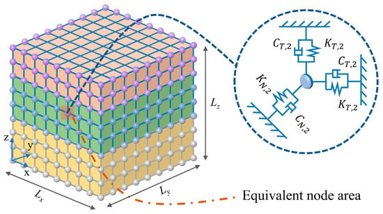
In layered soil, impedance contrasts between adjacent layers result from differences in density and wave speed. When seismic waves reach an interface between soil layers, wave energy is redistributed to satisfy displacement and stress continuity, generating reflected and transmitted waves. From the perspective of wavefield decomposition, the free field response in layered soil results from the superposition of incident, reflected, and transmitted waves rather than from a single incident wave alone. In SSI analysis, dynamic interaction of the structure and its foundation with the surrounding soil also generates reflected and scattered waves. In finite element analysis, truncating the semi-infinite soil domain into a finite computational domain may cause spurious reflections of outgoing waves if the truncation boundaries are not treated appropriately, thereby affecting the dynamic response within the domain. To represent the dynamic restraint of semi-infinite soil and radiation damping, a viscoelastic artificial boundary (VAB), consisting of parallel springs and dashpots, is assigned to the boundary nodes, as shown in Figure 1. The springs primarily provide boundary stiffness under low-frequency and quasi-static deformation, whereas the dashpots primarily absorb outgoing wave energy. The VAB parameters [11] are defined as follows:

$$K_{T,f}={\alpha }_T{\displaystyle \frac{G_f}{R}},C_{T,f}={\rho }_f{c}_{s,f},$$

(1)

$$K_{N,f}={\alpha }_N{\displaystyle \frac{G_f}{R}},C_{N,f}={\rho }_f{c}_{p,f},$$

(2)

where K and C denote the spring stiffness and damping coefficient, respectively; the subscripts T and N represent the tangential and normal directions, and f is the soil layer number, with soil layers numbered consecutively from bottom to top, such that layers f − 1 and f + 1 are the layers immediately below and above layer f, respectively; R is the distance from the wave source to the artificial boundary; α_T and α_N are correction coefficients, taken as 0.67 and 1.333, respectively, for three-dimensional problems; G_f is the shear modulus of the medium; ρ_f is the density; and c_s,f and c_p,f are the shear wave and compressional wave velocities of the foundation, respectively.

Figure 1. Viscoelastic boundary model.

For boundary nodes located at a soil-layer interface, the spring and dashpot contributions are calculated separately using the properties of the adjoining layers and then summed.

3. Proposed Seismic Input Method Based on the Path Cumulative Amplitude Coefficient

3.1. Seismic Input Formulation Under Vertical Incidence

To introduce seismic motion into the finite computational domain, the free-field displacement, velocity, and stress on the truncation boundary are transformed into equivalent nodal force (ENF) applied to the VAB nodes [34]. The ENF comprises the spring-dashpot compensation associated with the free-field motion and the traction induced by the free-field stress:

$${\mathit{F}}_k=({\mathit{K}}_k{\mathit{u}}_k^{\mathit{ff}}+{\mathit{C}}_k{\dot{\mathit{u}}}_k^{\mathit{ff}}+{\mathit{\sigma }}_k^{\mathit{ff}}\mathit{n})A_k,$$

(3)

where ${\mathit{u}}_k^{\mathit{ff}}={\left[\begin{array}{ccc}u& v& w\end{array}\right]}^T$, ${\dot{\mathit{u}}}_k^{\mathit{ff}}={\left[\begin{array}{ccc}\dot{u}& \dot{v}& \dot{w}\end{array}\right]}^T$ and ${\mathit{\sigma }}_k^{\mathit{ff}}$ are the free-field displacement, velocity, and stress tensor at node k, respectively. n is the outward unit normal vector, and A_k is the equivalent nodal area. For boundaries normal to the x-, y-, and z-axes, respectively, K_k = diag(K_N,K_T,K_T),diag(K_T,K_N,K_T),diag(K_T,K_T,K_N), and C_k is defined analogously using C_N and C_T.

Equation (3) constructs equivalent input loads from the free field response, whereas the actual motion of the boundary nodes is determined by the coupled soil-structure finite element model. Reflected and scattered waves generated by the structure and its foundation, together with their propagation, are computed as part of the overall dynamic response. Through free field load compensation, the viscoelastic boundary provides restoring and dissipative actions on the scattered motion, which is the difference between the actual and free field motions, thereby approximately representing the radiation of scattered-wave energy into the far field.

For an isotropic elastic medium, the free-field stress tensor ${\mathit{\sigma }}_k^{\mathit{ff}}$ is

$${\mathit{\sigma }}_k^{\mathit{ff}}=\lambda \left(\nabla \cdot {\mathit{u}}_k^{\mathit{ff}}\right)\mathbf{I}+\mu \left[\nabla {\mathit{u}}_k^{\mathit{ff}}+{\left(\nabla {\mathit{u}}_k^{\mathit{ff}}\right)}^T\right],$$

(4)

where I is the identity matrix, and λ and μ are the Lamé constants.

Because density and wave velocity generally increase with depth, upward-propagating waves are refracted toward the interface normal as they enter shallower, lower-velocity layers. Therefore, seismic waves approaching horizontally layered near-surface sites may be approximated as vertically incident under far-field or deep-source earthquakes [19].

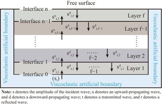
Conventional layered-foundation input methods generally retain only one reflection and one transmission in each soil layer, based on the short duration of earthquake excitation and energy dissipation in the foundation [18,20]. This simplification neglects the subsequent propagation of transmitted waves and the resulting cumulative amplitude and phase variations. The present method therefore retains a single reflection at each interface and the corresponding induced transmitted waves, while using the path cumulative amplitude coefficient for propagation-path selection and truncation, as shown in Figure 2.

Figure 2. Schematic illustration of seismic wave propagation under vertical incidence between different soil layers.

For vertically incident seismic waves, no mode conversion occurs at horizontal soil interfaces; only reflection and transmission alter the wave amplitude and phase. Taking S waves as an example, when an upgoing wave reaches the interface between soil layer f − 1 and soil layer f, the corresponding transmission and reflection coefficients are given by Equations (5) and (6).

$${A_{t,f}}^u={\displaystyle \frac{2}{z_{s,f}+1}},{A_{t,f}}^d={\displaystyle \frac{2z_{s,f+1}}{z_{s,f+1}+1}},$$

(5)

$${A_{r,f}}^u={\displaystyle \frac{z_{s,f}-1}{z_{s,f}+1}},{A_{r,f}}^d={\displaystyle \frac{1-z_{s,f+1}}{z_{s,f+1}+1}},$$

(6)

where A_t,f and A_r,f denote the transmission and reflection amplitude ratios, respectively, and the superscripts u and d indicate upgoing and downgoing waves. The S wave impedance ratio z_s,f is defined as

$$z_{s,f}={\displaystyle \frac{{\rho }_f{c}_{s,f}}{{\rho }_{f-1}{c}_{s,f-1}}}.$$

(7)

In layered soils, seismic waves undergo successive reflection and transmission at soil interfaces, generating multiple propagation paths. The amplitude of each wave component can be obtained by multiplying the amplitude variation coefficients along its corresponding path. Accordingly, the path cumulative amplitude coefficient Ψ is introduced to quantify the contribution of a given propagation path relative to the original incident wave. The proposed method retains a single reflection at each interface and the corresponding induced transmitted waves. When |Ψ| falls below a prescribed threshold ε, the contribution of the corresponding path is considered negligible, and further tracing of that path is terminated. In actual seismic-wave propagation, geometric spreading and material damping cause additional attenuation with increasing propagation distance. Therefore, neglecting sufficiently small-amplitude paths is also consistent with the physical attenuation characteristics of seismic waves in real sites. Accordingly, the cumulative amplitude coefficients for the upgoing transmitted, downgoing reflected, and downgoing transmitted wave components in soil layer f are expressed as follows:

$${\alpha }_{t,f}^u={\displaystyle \prod _{j=1}^f{A_{t,j}}^u},$$

(8)

$${\alpha }_{r,f}^d={\displaystyle \prod _{j=1}^f{A_{t,j}}^u}\times {A_{r,f}}^d,$$

(9)

$${\alpha }_{t,f}^d={\displaystyle \sum _{k=1}^{n-f}{\displaystyle \sum _{l=f+1}^n{\displaystyle {\displaystyle \prod _{j=1}^l}{A_{t,j}}^u}\times {A_{r,l}}^d\times {\displaystyle {\displaystyle \prod _{j=f}^n}{A_{t,j}}^d}}},$$

(10)

$${\mathrm{\Psi }}_{r,f}={\alpha }_{r,f}^d\times {\displaystyle {\displaystyle \prod ^{>\frac{\epsilon }{{\alpha }_{r,f}^d}}}({A_{r,f}}^u{A_{r,f}}^d)},{\mathrm{\Psi }}_{t,f}={\alpha }_{t,f}\times {\displaystyle {\displaystyle \prod ^{>\frac{\epsilon }{{\alpha }_{t,f}}}}({A_{r,f}}^u{A_{r,f}}^d)}.$$

(11)

For a x-direction S wave under vertical incidence, the free-field displacement vector is ${\mathit{u}}_k^{\mathit{ff}}={\left[\begin{array}{ccc}{u}_0(t)& 0& 0\end{array}\right]}^T$, and the corresponding velocity vector is ${\dot{\mathit{u}}}_k^{\mathit{ff}}={\left[\begin{array}{ccc}{\dot{u}}_0(t)& 0& 0\end{array}\right]}^T$. For any point O in Layer f, the displacement and velocity at an arbitrary time can be expressed as

$$u(t)={\alpha }_{t,f}^u{u}_0(t-\Delta {t_{\mathit{st},f}}^u)+{\alpha }_{r,f}^d{u}_0(t-\Delta {t_{\mathit{sr},f}}^d)+{\alpha }_{t,f}^d{u}_0(t-\Delta {t_{\mathit{st},f,k}}^d)+{\displaystyle \sum ^{\left|{\mathrm{\Psi }}_f>\epsilon \right|}{\mathrm{\Psi }}_f{u}_0(t-\Delta t_{s\mathrm{\Psi }})},$$

(12)

$$\dot{u}(t)={\alpha }_{t,f}^u{\dot{u}}_0(t-\Delta {t_{\mathit{st},f}}^u)+{\alpha }_{r,f}^d{\dot{u}}_0(t-\Delta {t_{\mathit{sr},f}}^d)+{\alpha }_{t,f}^d{\dot{u}}_0(t-\Delta {t_{\mathit{st},f,k}}^d)+{\displaystyle \sum ^{\left|{\mathrm{\Psi }}_f>\epsilon \right|}{\mathrm{\Psi }}_f{\dot{u}}_0(t-\Delta t_{s\mathrm{\Psi }})}.$$

(13)

where Δt_sΨ denotes the delay time associated with the S wave propagation path corresponding to the cumulative amplitude coefficient; Δt_st,f is the delay time for the transmitted wave to reach the point; and Δt_sr,f is the delay time for the reflected wave to reach the point.

$$\Delta {t_{\mathit{st},f}}^u={\displaystyle \sum _{j=1}^{f-1}\frac{h_j}{c_{s,j}}}+{\displaystyle \frac{d_f}{c_{s,f}}},$$

(14)

$$\Delta {t_{\mathit{sr},f}}^d={\displaystyle \sum _{j=1}^{f-1}\frac{h_j}{c_{s,j}}}+{\displaystyle \frac{2h_f-d_f}{c_{s,f}}},$$

(15)

$$\Delta {t_{\mathit{st},f,k}}^d={\displaystyle {\displaystyle \sum _{j=1}^{f-1}}\frac{h_j}{c_{s,j}}}+{\displaystyle {\displaystyle \sum _{i=0}^k}\frac{2h_{f+i}}{c_{s,f+i}}}-{\displaystyle \frac{d_f}{c_{s,f}}},$$

(16)

where h_f is the thickness of soil layer f, and d_f is the vertical distance between node O and the bottom boundary of Layer f.

Accordingly, the stress tensor ${\mathit{\sigma }}_k^{\mathit{ff}}$ in Equation (4) can be reduced to:

$${\mathit{\sigma }}_k^{\mathit{ff}}=\left[\begin{array}{ccc}& & {\rho }_f{c}_{s,f}^2{\displaystyle \frac{\partial u}{\partial z}}\\ & & \\ {\rho }_f{c}_{s,f}^2{\displaystyle \frac{\partial u}{\partial z}}& & \end{array}\right],$$

(17)

$${\displaystyle \frac{\partial u}{\partial z}}=-{\displaystyle \frac{1}{c_{s,f}}}\left[{\alpha }_{t,f}^u{\dot{u}}_0(t-\Delta {t_{\mathit{st},f}}^u)-{\alpha }_{r,f}^d{\dot{u}}_0(t-\Delta {t_{\mathit{sr},f}}^d)-{\alpha }_{t,f}^d{\dot{u}}_0(t-\Delta {t_{\mathit{st},f,k}}^d)\pm {\displaystyle \sum ^{{\mathrm{\Psi }}_f>\epsilon }{\mathrm{\Psi }}_f{\dot{u}}_0(t-\Delta t_{s\mathrm{\Psi }})}\right]$$

(18)

Substituting Equations (12)–(18) into Equation (3) yields the ENF on the five surfaces of the VAB for vertically incident S waves polarized in the x-direction.

For node O_−x on the negative x-direction boundary (x = 0), the ENF is expressed as follows:

$$\begin{array}{l}{F}_{-\mathit{xx}}=\left\{\begin{array}{l}{K}_{N,f}\left[{\alpha }_{t,f}^u{u}_0(t-\Delta {t_{\mathit{st},f}}^u)+{\alpha }_{r,f}^d{u}_0(t-\Delta {t_{\mathit{sr},f}}^d)+{\alpha }_{t,f}^d{u}_0(t-\Delta {t_{\mathit{st},f,k}}^d)+{\displaystyle \sum ^{{\mathrm{\Psi }}_f>\epsilon }{\mathrm{\Psi }}_f{u}_0(t-\Delta t_{s\mathrm{\Psi }})}\right]\\ +C_{N,f}\left[{\alpha }_{t,f}^u{\dot{u}}_0(t-\Delta {t_{\mathit{st},f}}^u)+{\alpha }_{r,f}^d{\dot{u}}_0(t-\Delta {t_{\mathit{sr},f}}^d)+{\alpha }_{t,f}^d{\dot{u}}_0(t-\Delta {t_{\mathit{st},f,k}}^d)+{\displaystyle \sum ^{{\mathrm{\Psi }}_f>\epsilon }{\mathrm{\Psi }}_f{\dot{u}}_0(t-\Delta t_{s\mathrm{\Psi }})}\right]\end{array}\right\}{A}_k\\ F_{-\mathit{xy}}=0\\ F_{-\mathit{xz}}={\rho }_f{c}_{s,f}\left[{\alpha }_{t,f}^u{\dot{u}}_0(t-\Delta {t_{\mathit{st},f}}^u)-{\alpha }_{r,f}^d{\dot{u}}_0(t-\Delta {t_{\mathit{sr},f}}^d)-{\alpha }_{t,f}^d{\dot{u}}_0(t-\Delta {t_{\mathit{st},f,k}}^d)\pm {\displaystyle \sum ^{{\mathrm{\Psi }}_f>\epsilon }{\mathrm{\Psi }}_f{\dot{u}}_0(t-\Delta t_{s\mathrm{\Psi }})}\right]A_k\end{array}.$$

(19)

For node O_x on the positive x-direction boundary (x = L_x), the ENF is given by:

$$\begin{array}{l}{F}_{\mathit{xx}}=F_{-\mathit{xx}}\\ F_{\mathit{xy}}=0\\ F_{\mathit{xz}}=-F_{-\mathit{xz}}\end{array}.$$

(20)

For node O_−y on the negative y-direction boundary (y = 0), the ENF is given by:

$$\begin{array}{l}{F}_{-\mathit{yx}}=\left\{\begin{array}{l}{K}_{T,f}\left[{\alpha }_{t,f}^u{u}_0(t-\Delta {t_{\mathit{st},f}}^u)+{\alpha }_{r,f}^d{u}_0(t-\Delta {t_{\mathit{sr},f}}^d)+{\alpha }_{t,f}^d{u}_0(t-\Delta {t_{\mathit{st},f,k}}^d)+{\displaystyle \sum ^{{\mathrm{\Psi }}_f>\epsilon }{\mathrm{\Psi }}_f{u}_0(t-\Delta t_{s\mathrm{\Psi }})}\right]\\ +C_{T,f}\left[{\alpha }_{t,f}^u{\dot{u}}_0(t-\Delta {t_{\mathit{st},f}}^u)+{\alpha }_{r,f}^d{\dot{u}}_0(t-\Delta {t_{\mathit{sr},f}}^d)+{\alpha }_{t,f}^d{\dot{u}}_0(t-\Delta {t_{\mathit{st},f,k}}^d)+{\displaystyle \sum ^{{\mathrm{\Psi }}_f>\epsilon }{\mathrm{\Psi }}_f{\dot{u}}_0(t-\Delta t_{s\mathrm{\Psi }})}\right]\end{array}\right\}{A}_k\\ F_{-\mathit{yy}}=0\\ F_{-\mathit{yz}}=0\end{array}.$$

(21)

For node O_y on the positive y-direction boundary (y = L_y), the ENF is given by:

$$\begin{array}{l}{F}_{\mathit{yx}}=F_{-\mathit{yx}}\\ F_{\mathit{yy}}=0\\ F_{\mathit{yz}}=0\end{array}.$$

(22)

For node O_z on the bottom boundary (z = 0), the ENF is given by:

$$\begin{array}{l}{F}_{-\mathit{zx}}=\left\{\begin{array}{l}{K}_{T,1}\left[{\alpha }_{t,1}^u{u}_0(t-\Delta {t_{\mathit{st},1}}^u)+{\alpha }_{r,1}^d{u}_0(t-\Delta {t_{\mathit{sr},1}}^d)+{\alpha }_{t,1}^d{u}_0(t-\Delta {t_{\mathit{st},1,k}}^d)+{\displaystyle \sum ^{{\mathrm{\Psi }}_1>\epsilon }{\mathrm{\Psi }}_1{u}_0(t-\Delta t_{s\mathrm{\Psi }})}\right]\\ +C_{T,2}\left[{\alpha }_{t,1}^u{\dot{u}}_0(t-\Delta {t_{\mathit{st},1}}^u)+{\alpha }_{r,1}^d{\dot{u}}_0(t-\Delta {t_{\mathit{sr},1}}^d)+{\alpha }_{t,1}^d{\dot{u}}_0(t-\Delta {t_{\mathit{st},1,k}}^d)+{\displaystyle \sum ^{{\mathrm{\Psi }}_1>\epsilon }{\mathrm{\Psi }}_1{\dot{u}}_0(t-\Delta t_{s\mathrm{\Psi }})}\right]\\ +{\rho }_1{c}_{s,1}\left[{\alpha }_{t,1}^u{\dot{u}}_0(t-\Delta {t_{\mathit{st},1}}^u)-{\alpha }_{r,1}^d{\dot{u}}_0(t-\Delta {t_{\mathit{sr},1}}^d)-{\alpha }_{t,1}^d{\dot{u}}_0(t-\Delta {t_{\mathit{st},1,k}}^d)\pm {\displaystyle \sum ^{{\mathrm{\Psi }}_1>\epsilon }{\mathrm{\Psi }}_1{\dot{u}}_0(t-\Delta t_{s\mathrm{\Psi }})}\right]\end{array}\right\}{A}_k\\ F_{-\mathit{zy}}=0\\ F_{-\mathit{zz}}=0\end{array}.$$

(23)

In the subscript of the equivalent nodal force, the first letter denotes the outward normal direction of the boundary surface on which the node is located, while the second letter denotes the component direction of the force.

The calculation procedures for vertically incident S waves in the y-direction and vertically incident P waves are analogous.

3.2. Seismic Input Formulation Under Oblique Incidence

For far-field or deep-source earthquakes, seismic waves can often be approximated as vertically incident waves. In reality, however, seismic waves are not always strictly vertical when they arrive at engineering sites. In addition, P and SV waves undergo more complex reflection, transmission, and mode conversion at soil layer interfaces, thereby altering the free field response of the foundation, as shown in Figure 3. If only the vertical incidence assumption is adopted, the wave propagation characteristics in actual sites and their influence on the structural dynamic response may not be fully represented. Therefore, based on the vertical incidence formulation, this section further derives the seismic input method under oblique incidence conditions.

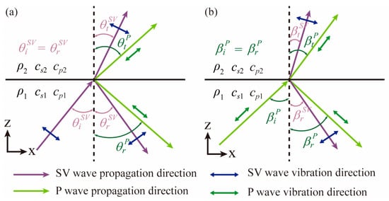
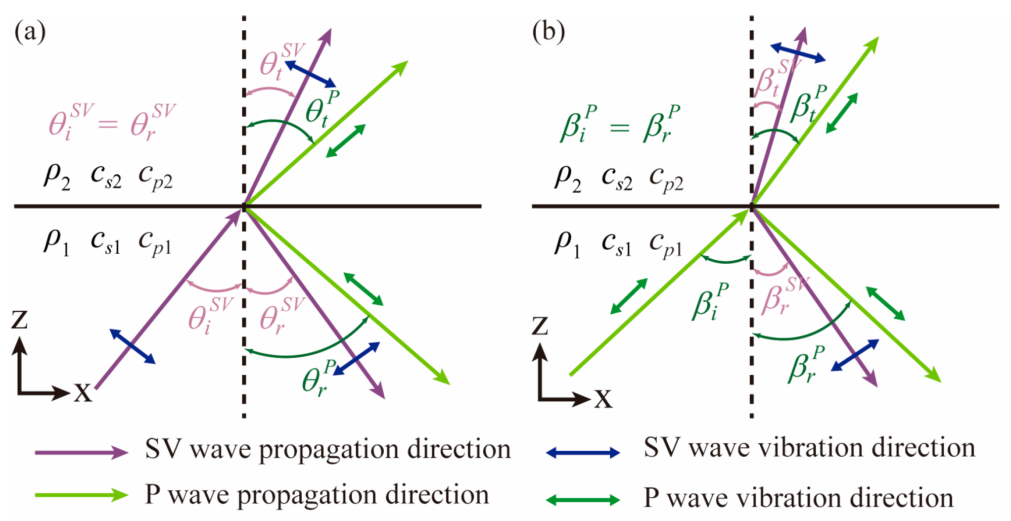
Figure 3. Schematic illustration of reflection and transmission under oblique incidence of different waves: (a) obliquely incident SV wave; (b) obliquely incident P wave.

3.2.1. Reflection and Transmission Coefficients

This study considers wave propagation at angles below the critical incidence angle, such that all reflected, transmitted, and converted components remain propagating. The applicable range of incidence angles is determined jointly by the incident wave type and the wave speeds in the individual layers. Under these conditions, when an incident SV wave propagates from soil-1 to soil-2 and reaches the layer interface, as shown in Figure 3a, the incident wave energy is redistributed at the interface because of the difference in wave impedance. Consequently, a reflected SV wave, a reflected P wave, a transmitted SV wave, and a transmitted P wave are generated. According to Snell’s law, the horizontal slowness of each wave mode along the interface must remain identical. Therefore

$${\displaystyle \frac{\sin {\theta }_i^{\mathit{SV}}}{c_{s,1}}}={\displaystyle \frac{\sin {\theta }_r^P}{c_{p,1}}}={\displaystyle \frac{\sin {\theta }_t^{\mathit{SV}}}{c_{s,2}}}={\displaystyle \frac{\sin {\theta }_t^P}{c_{p,2}}},$$

(24)

where ${\theta }_i^{\mathit{SV}}$ is the angle between the incident SV wave and the interface normal; ${\theta }_r^P$, ${\theta }_t^{\mathit{SV}}$, and ${\theta }_t^P$ are the propagation angles of the reflected P wave, transmitted SV wave, and transmitted P wave, respectively. Since the reflected SV wave and the incident SV wave are in the same medium and have the same wave velocity, the reflection angle of the reflected SV wave is equal to the incident angle.

Enforcing continuity of the normal and tangential displacements and stresses across the interface gives the amplitude ratios of the reflected and transmitted waves:

$$\left[\begin{array}{cccc}\cos {\theta }_i^{\mathit{SV}}& \sin {\theta }_r^P& -\cos {\theta }_t^{\mathit{SV}}& -\sin {\theta }_t^P\\ \sin {\theta }_i^{\mathit{SV}}& -\cos {\theta }_r^P& \sin {\theta }_t^{\mathit{SV}}& -\cos {\theta }_t^P\\ -\cos 2{\theta }_i^{\mathit{SV}}& -{\displaystyle \frac{c_{s,1}}{c_{p,1}}}\sin 2{\theta }_r^P& -{\displaystyle \frac{{\rho }_2{c}_{s,2}}{{\rho }_1{c}_{s,1}}}\cos 2{\theta }_t^{\mathit{SV}}& -{\displaystyle \frac{{\rho }_2{c}_{s,2}^2}{{\rho }_1{c}_{p,2}{c}_{s,1}}}\sin 2{\theta }_t^P\\ -\sin 2{\theta }_i^{\mathit{SV}}& {\displaystyle \frac{c_{p,1}}{c_{s,1}}}\cos 2{\theta }_i^{\mathit{SV}}& {\displaystyle \frac{{\rho }_2{c}_{s,2}}{{\rho }_1{c}_{s,1}}}\sin 2{\theta }_t^{\mathit{SV}}& -{\displaystyle \frac{{\rho }_2{c}_{p,2}}{{\rho }_1{c}_{s,1}}}\cos 2{\theta }_t^{\mathit{SV}}\end{array}\right]\left[\begin{array}{c}{A}_r^{\mathit{SV},d}\\ A_r^{P,d}\\ A_t^{\mathit{SV},u}\\ A_t^{P,u}\end{array}\right]=\left[\begin{array}{c}-\cos {\theta }_i^{\mathit{SV}}\\ \sin {\theta }_i^{\mathit{SV}}\\ -\cos 2{\theta }_i^{\mathit{SV}}\\ \sin 2{\theta }_i^{\mathit{SV}}\end{array}\right],$$

(25)

where $A_r^{\mathit{SV},d}$, $A_r^{P,d}$, $A_t^{\mathit{SV},u}$, and $A_t^{P,u}$ denote the amplitude ratios of the reflected SV wave, reflected P wave, transmitted SV wave, and transmitted P wave to the incident SV wave, respectively. The superscript u denotes an upgoing wave, whereas d denotes a downgoing wave. Their expressions are given as follows:

$$\begin{array}{c}{A}_r^{\mathit{SV},d}=-1+{\displaystyle \frac{-A_r^{P,d}\sin {\theta }_r^P+A_t^{\mathit{SV},u}\cos {\theta }_t^{\mathit{SV}}+A_t^{P,u}\sin {\theta }_t^P}{\cos {\theta }_i^{\mathit{SV}}}}\\ A_r^{P,d}=a_1+a_2{A}_t^{\mathit{SV},u}+a_3{A}_t^{P,u}\\ A_t^{\mathit{SV},u}={\displaystyle \frac{a_6{a}_8-a_5{a}_9}{a_4{a}_8-a_5{a}_7}}\\ A_t^{P,u}={\displaystyle \frac{a_4{a}_9-a_6{a}_7}{a_4{a}_8-a_5{a}_7}}\end{array},$$

(26)

where a_j denotes the algebraic coefficient of the expression, as given in Appendix A.

When the upper boundary is a free surface, the amplitude ratios of the reflected waves to the incident wave reduce to:

$$\begin{array}{c}{A}_r^{\mathit{SV},\mathit{free}}={\displaystyle \frac{c_{p,1}^2{\cos }^{2}2{\theta }_i^{\mathit{SV}}-c_{s,1}^2\sin 2{\theta }_i^{\mathit{SV}}\sin 2{\theta }_r^P}{c_{p,1}^2{\cos }^{2}2{\theta }_i^{\mathit{SV}}+c_{s,1}^2\sin 2{\theta }_i^{\mathit{SV}}\sin 2{\theta }_r^P}}\\ A_r^{P,\mathit{free}}={\displaystyle \frac{2c_{s,1}{c}_{p,1}\sin 2{\theta }_i^{\mathit{SV}}\cos 2{\theta }_i^{\mathit{SV}}}{c_{p,1}^2{\cos }^{2}2{\theta }_i^{\mathit{SV}}+c_{s,1}^2\sin 2{\theta }_i^{\mathit{SV}}\sin 2{\theta }_r^P}}\end{array}.$$

(27)

For an obliquely incident P wave (Figure 3b), the reflection and transmission coefficients are derived in the same manner from Snell’s law and the displacement and stress continuity conditions:

$$\left[\begin{array}{cccc}\sin {\beta }_i^P& \cos {\beta }_r^{\mathit{SV}}& -\sin {\beta }_t^P& -\cos {\beta }_t^{\mathit{SV}}\\ -\cos {\beta }_i^P& \sin {\beta }_r^{\mathit{SV}}& -\cos {\beta }_t^P& \sin {\beta }_t^{\mathit{SV}}\\ -\sin 2{\beta }_i^P& -{\displaystyle \frac{c_{p,1}}{c_{s,1}}}\cos 2{\beta }_r^{\mathit{SV}}& -{\displaystyle \frac{{\rho }_2{c}_{s,2}^2{c}_{p,1}}{{\rho }_1{c}_{s,1}^2{c}_{p,2}}}\sin 2{\beta }_t^P& -{\displaystyle \frac{{\rho }_2{c}_{s,2}{c}_{p,1}}{{\rho }_1{c}_{s,1}^2}}\cos 2{\beta }_t^{\mathit{SV}}\\ \cos 2{\beta }_r^{\mathit{SV}}& -{\displaystyle \frac{c_{s,1}}{c_{p,1}}}\sin 2{\beta }_r^{\mathit{SV}}& -{\displaystyle \frac{{\rho }_2{c}_{p,2}}{{\rho }_1{c}_{p,1}}}\cos 2{\beta }_t^{\mathit{SV}}& {\displaystyle \frac{{\rho }_2{c}_{s,2}}{{\rho }_1{c}_{p,1}}}\sin 2{\beta }_t^{\mathit{SV}}\end{array}\right]\left[\begin{array}{c}{B}_r^{P,d}\\ B_r^{\mathit{SV},d}\\ B_t^{P,u}\\ B_t^{\mathit{SV},u}\end{array}\right]=\left[\begin{array}{c}-\sin {\beta }_i^P\\ -\cos {\beta }_i^P\\ -\sin 2{\beta }_i^P\\ -\cos 2{\beta }_r^{\mathit{SV}}\end{array}\right],$$

(28)

where $B_r^{P,d}$, $B_r^{\mathit{SV},d}$, $B_t^{P,u}$, and $B_t^{\mathit{SV},u}$ denote the amplitude ratios of the reflected P wave, reflected SV wave, transmitted P wave, and transmitted SV wave to the incident P wave, respectively. The superscript u denotes an upgoing wave, whereas d denotes a downgoing wave. Their expressions are given as follows:

$$\begin{array}{c}{B}_r^{P,d}=-1+{\displaystyle \frac{-B_r^{\mathit{SV},d}\cos {\beta }_r^{\mathit{SV}}+B_t^{P,u}\sin {\beta }_t^P+B_t^{\mathit{SV},u}\cos {\beta }_t^{\mathit{SV}}}{\sin {\beta }_i^P}}\\ B_r^{\mathit{SV},d}=b_1+b_2{B}_t^{P,u}+b_3{B}_t^{\mathit{SV},u}\\ B_t^{P,u}={\displaystyle \frac{b_6{b}_8-b_5{b}_9}{b_4{b}_8-b_5{b}_7}}\\ B_t^{\mathit{SV},u}={\displaystyle \frac{b_4{b}_9-b_6{b}_7}{b_4{b}_8-b_5{b}_7}}\end{array},$$

(29)

where b_j denotes the algebraic coefficient of the expression, as given in Appendix A.

For an obliquely incident P wave, when the upper boundary is a free surface, the corresponding reflection coefficients reduce to:

$$\begin{array}{c}{B}_r^{P,\mathit{free}}={\displaystyle \frac{c_{s,1}^2\sin 2{\beta }_i^P\sin 2{\beta }_r^{\mathit{SV}}-c_{p,1}^2{\cos }^{2}2{\beta }_r^{\mathit{SV}}}{c_{s,1}^2\sin 2{\beta }_i^P\sin 2{\beta }_r^{\mathit{SV}}+c_{p,1}^2{\cos }^{2}2{\beta }_r^{\mathit{SV}}}}\\ B_r^{\mathit{SV},\mathit{free}}={\displaystyle \frac{2c_{s,1}{c}_{p,1}\sin 2{\beta }_i^P\cos 2{\beta }_r^{\mathit{SV}}}{c_{s,1}^2\sin 2{\beta }_i^P\sin 2{\beta }_r^{\mathit{SV}}+c_{p,1}^2{\cos }^{2}2{\beta }_r^{\mathit{SV}}}}\end{array}.$$

(30)

The coefficients for propagation from soil-2 to soil-1 are obtained analogously using the corresponding material properties and propagation angles.

For both obliquely incident SV waves and P waves, the path cumulative amplitude coefficient Ψ can be expressed as:

$$\mathrm{\Psi }={\displaystyle \prod A_t{B}_t}{\displaystyle \prod A_r{B}_r}.$$

(31)

3.2.2. Free Field Response Under Oblique Incidence

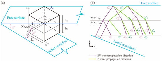
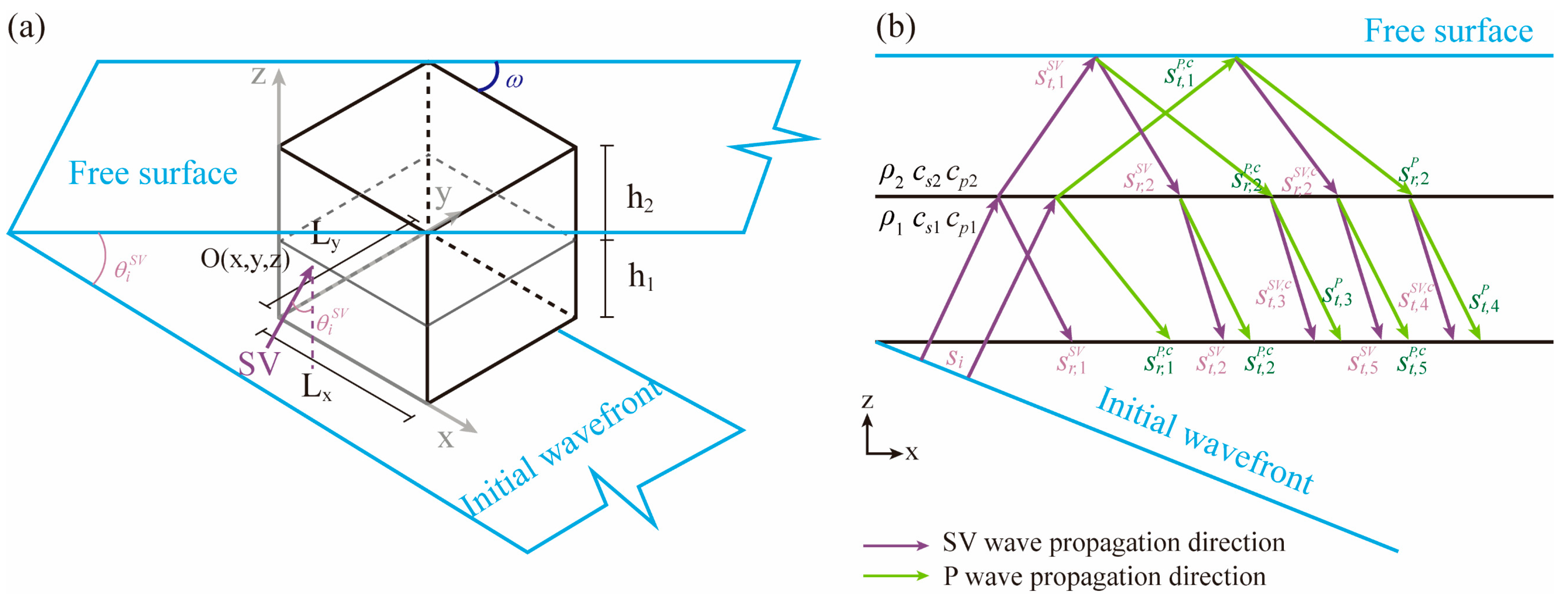
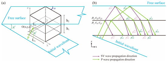
Taking a two-layer soil profile as an example, Figure 4a illustrates the free field under obliquely incident SV waves. The incident angle θ is defined between the propagation direction and the positive z-axis, while the azimuth angle ω is measured between its horizontal projection and the positive x-axis. Assuming that the initial wavefront passes through the origin at t = 0, the incident SV wave displacement history is denoted by s_i(t), and its contribution at an arbitrary point O(x,y,z) is expressed as s_i(t_s0). As shown in Figure 4b, each wave component generated by reflection, transmission, and mode conversion is constructed by multiplying the amplitude coefficients along its propagation path and introducing the corresponding time delay. Its contribution can therefore be expressed in the general form ΠA_jB_js_i(t_sk), with propagation-path retention and truncation governed by the path cumulative amplitude coefficient Ψ. The amplitude expressions for the individual wave components are given in Table A1 of Appendix B.

Figure 4. Schematic illustration of the free field in a semi-infinite medium under obliquely incident SV waves: (a) three-dimensional free field in a semi-infinite medium; (b) composition of the site motion.

Accordingly, the free-field displacement components in the lower soil layer can be expressed as:

$$\left[\begin{array}{c}u\left(t\right)\\ v\left(t\right)\\ w\left(t\right)\end{array}\right]=\left[\begin{array}{cccc}\cos {\theta }_i^{\mathit{SV}}\cos \omega & \cos {\theta }_i^{\mathit{SV}}\cos \omega & \sin {\theta }_r^P\cos \omega & (\cos {\theta }_i^{\mathit{SV}}+\sin {\theta }_r^P)\cos \omega \\ \cos {\theta }_i^{\mathit{SV}}\sin \omega & \cos {\theta }_i^{\mathit{SV}}\sin \omega & \sin {\theta }_r^P\sin \omega & (\cos {\theta }_i^{\mathit{SV}}+\sin {\theta }_r^P)\sin \omega \\ -\sin {\theta }_i^{\mathit{SV}}& \sin {\theta }_i^{\mathit{SV}}& -\cos {\theta }_r^P& \sin {\theta }_i^{\mathit{SV}}-\cos {\theta }_r^P\end{array}\right]\left[\begin{array}{c}{s}_i\left(t_{s0}\right)\\ s_{r,1}^{\mathit{SV}}\left(t_{s1}\right)+s_{t,2}^{\mathit{SV}}\left(t_{s9}\right)+s_{t,3}^{\mathit{SV},c}\left(t_{s11}\right)+s_{t,4}^{\mathit{SV},c}\left(t_{s13}\right)+s_{t,5}^{\mathit{SV}}\left(t_{s15}\right)\\ s_{r,1}^P\left(t_{s2}\right)+s_{t,2}^{P,c}\left(t_{s10}\right)+s_{t,3}^P\left(t_{s12}\right)+s_{t,4}^P\left(t_{s14}\right)+s_{t,5}^{P,c}\left(t_{s16}\right)\\ {\displaystyle \sum \mathrm{\Psi }{s}_i\left(t_{s\mathrm{\Psi }}\right)}\end{array}\right]$$

(32)

The free-field displacement components in the upper soil layer can be expressed as:

$$\left[\begin{array}{c}u\left(t\right)\\ v\left(t\right)\\ w\left(t\right)\end{array}\right]=\left[\begin{array}{ccccc}\cos {\theta }_t^{\mathit{SV}}\cos \omega & \sin {\theta }_t^P\cos \omega & \cos {\theta }_t^{\mathit{SV}}\cos \omega & \sin {\theta }_t^P\cos \omega & (\cos {\theta }_t^{\mathit{SV}}+\sin {\theta }_t^P)\cos \omega \\ \cos {\theta }_t^{\mathit{SV}}\sin \omega & \sin {\theta }_t^P\sin \omega & \cos {\theta }_t^{\mathit{SV}}\sin \omega & \sin {\theta }_t^P\sin \omega & (\cos {\theta }_t^{\mathit{SV}}+\sin {\theta }_t^P)\cos \omega \\ -\sin {\theta }_t^{\mathit{SV}}& \cos {\theta }_t^P& \sin {\theta }_t^{\mathit{SV}}& -\cos {\theta }_t^P& \pm \sin {\theta }_t^{\mathit{SV}}\pm \cos {\theta }_t^P\end{array}\right]\left[\begin{array}{c}{s}_{t,1}^{\mathit{SV}}\left(t_{s3}\right)\\ s_{t,1}^{P,c}\left(t_{s4}\right)\\ s_{r,2}^{\mathit{SV}}\left(t_{s5}\right)+s_{r,2}^{\mathit{SV},c}\left(t_{s7}\right)\\ s_{r,2}^{P,c}\left(t_{s6}\right)+s_{r,2}^P\left(t_{s8}\right)\\ {\displaystyle \sum \mathrm{\Psi }{s}_i\left(t_{s\mathrm{\Psi }}\right)}\end{array}\right],$$

(33)

where t_sk denotes the corrected time at which the corresponding wave component reaches an arbitrary point O(x,y,z), which can be expressed as t − Δt_sk. Here, Δt_sk represents the propagation time delay associated with the corresponding propagation path. The detailed expressions for the time delays of all propagation paths on the five boundary surfaces are provided in Appendix B.

Similarly, for obliquely incident P waves, the free field can also be constructed using the path-tracing method together with the cumulative multiplication of amplitude variation coefficients, as illustrated in Figure 5. Let the displacement time history of the incident P wave be p_i(t), with the incident angle denoted by β and the azimuth angle by ω. Since the particle motion of a P wave is parallel to its propagation direction, the P wave component corresponding to each propagation path, ΠB_jA_jp_i(t_pk), can be directly projected onto the x-, y-, and z-directions. The retention and truncation of wave components are likewise governed by the path cumulative amplitude coefficient Ψ. The amplitude expressions for the individual wave components are given in Table A1 of Appendix B.

Figure 5. Schematic illustration of the free field in a semi-infinite medium under obliquely incident P waves: (a) three-dimensional free field in a semi-infinite medium; (b) composition of the site motion.

The free-field displacement components in the lower and upper soil layers are therefore expressed as:

$$\left[\begin{array}{c}u\left(t\right)\\ v\left(t\right)\\ w\left(t\right)\end{array}\right]=\left[\begin{array}{cccc}\sin {\beta }_i^P\cos \omega & \sin {\beta }_i^P\cos \omega & \cos {\beta }_r^{\mathit{SV}}\cos \omega & (\sin {\beta }_i^P+\cos {\beta }_r^{\mathit{SV}})\cos \omega \\ \sin {\beta }_i^P\sin \omega & \sin {\beta }_i^P\sin \omega & \cos {\beta }_r^{\mathit{SV}}\sin \omega & (\sin {\beta }_i^P+\cos {\beta }_r^{\mathit{SV}})\sin \omega \\ \cos {\beta }_i^P& -\cos {\beta }_i^P& \sin {\beta }_r^{\mathit{SV}}& \sin {\beta }_r^{\mathit{SV}}-\cos {\beta }_i^P\end{array}\right]\left[\begin{array}{c}{p}_i\left(t_{p0}\right)\\ p_{r,1}^P\left(t_{p1}\right)+p_{t,2}^P\left(t_{p9}\right)+p_{t,3}^{P,c}\left(t_{p11}\right)+p_{t,4}^{P,c}\left(t_{p13}\right)+p_{t,5}^P\left(t_{p15}\right)\\ p_{r,1}^{\mathit{SV}}\left(t_{p2}\right)+p_{t,2}^{\mathit{SV},c}\left(t_{p10}\right)+p_{t,3}^{\mathit{SV}}\left(t_{p12}\right)+p_{t,4}^{\mathit{SV}}\left(t_{p14}\right)+p_{t,5}^{\mathit{SV},c}\left(t_{p16}\right)\\ {\displaystyle \sum \mathrm{\Psi }{p}_i\left(t_{p\mathrm{\Psi }}\right)}\end{array}\right]$$

(34)

$$\left[\begin{array}{c}u\left(t\right)\\ v\left(t\right)\\ w\left(t\right)\end{array}\right]=\left[\begin{array}{ccccc}\sin {\beta }_t^P\cos \omega & \cos {\beta }_t^{\mathit{SV}}\cos \omega & \sin {\beta }_t^P\cos \omega & \cos {\beta }_t^{\mathit{SV}}\cos \omega & (\sin {\beta }_t^P+\cos {\beta }_t^{\mathit{SV}})\cos \omega \\ \sin {\beta }_t^P\sin \omega & \cos {\beta }_t^{\mathit{SV}}\sin \omega & \sin {\beta }_t^P\sin \omega & \cos {\beta }_t^{\mathit{SV}}\sin \omega & (\sin {\beta }_t^P+\cos {\beta }_t^{\mathit{SV}})\sin \omega \\ \cos {\beta }_t^P& -\sin {\beta }_t^{\mathit{SV}}& -\cos {\beta }_t^P& \sin {\beta }_t^{\mathit{SV}}& \pm \sin {\beta }_t^{\mathit{SV}}\pm \cos {\beta }_t^P\end{array}\right]\left[\begin{array}{c}{p}_{t,1}^P\left(t_{p3}\right)\\ p_{t,1}^{\mathit{SV},c}\left(t_{p4}\right)\\ p_{r,2}^P\left(t_{p5}\right)+p_{r,2}^{P,c}\left(t_{p7}\right)\\ p_{r,2}^{\mathit{SV},c}\left(t_{p6}\right)+p_{r,2}^{\mathit{SV}}\left(t_{p8}\right)\\ {\displaystyle \sum \mathrm{\Psi }{p}_i\left(t_{p\mathrm{\Psi }}\right)}\end{array}\right],$$

(35)

where t_pk has the same definition as t_sk. The corresponding propagation time delay Δt_pk can be obtained from the geometric relationships of the obliquely incident wave propagation paths given in Appendix B by replacing the propagation angles and wave velocities of the SV wave with the corresponding parameters of the P wave.

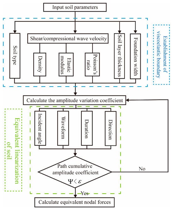
By substituting Equations (32)–(35) into the ENF formulations in Equations (3) and (4), the ENF applied to the boundary nodes of the model during obliquely incident seismic wave input in layered soil with VAB can be obtained. Following the procedure shown in Figure 6, automated seismic input in Abaqus 2021 can be achieved through MATLAB R2024a and Python 2.7.15 implementations.

Figure 6. Flowchart of the ENF calculation procedure.

4. Numerical Validation and Analysis

4.1. Harmonic Wave Validation

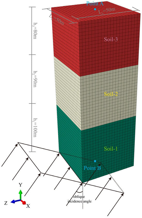
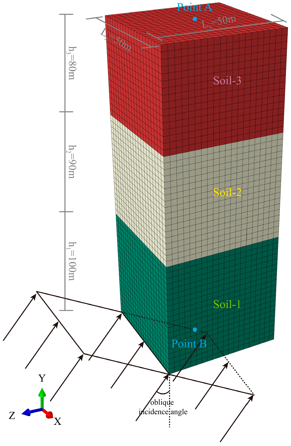
To verify the implementation accuracy of the proposed VAB and ENF input method for layered soil, an independent three-dimensional layered soil model consisting of three soil layers was established, as shown in Figure 7, where Y is vertical and X and Z are horizontal. The model was extracted from a three-dimensional semi-infinite domain with a plan dimension of 100 m × 100 m and a depth of 270 m. The ground surface was modeled as a free surface. From top to bottom, the three soil layers have thicknesses of 80, 90, and 100 m, respectively, and their material properties are listed in Table 1. An automated program was developed using MATLAB and Python to generate the Abaqus .inp file, enabling efficient implementation of the VAB and ENF on the bottom boundary and the four lateral boundaries. Different incident wave types were applied at the model base, including vertically incident SV waves (with particle motion along X) and P waves, as well as obliquely incident SV and P waves at both 10° and 20°. For the obliquely incident SV waves, the horizontal particle-motion component was aligned with X. In path tracing, the cumulative amplitude coefficient Ψ_r represents the amplitude contribution of the rth path relative to the initial incident wave, and a dimensionless truncation threshold of ε = 0.001 is adopted. Whenever a new propagation branch is generated, it is retained and traced further only if it satisfies |Ψ_r| ≥ ε. All examples in this study use converged semi-analytical free field solutions for the corresponding incidence conditions as theoretical references. These solutions satisfy displacement and stress continuity at layer interfaces and the traction-free condition at the free surface. They are constructed by summing contributions up to the 50th order of interface scattering without pruning based on individual path amplitude ratios, and are verified by increasing the scattering order and comparing the results with independently computed frequency-domain solutions [35,36]. The displacement time history of the incident wave is given by:

$$u(t)={\displaystyle \frac{1-\cos (10\pi t)}{2}},t\in \left[0,0.2\right].$$

(36)

Figure 7. Schematic illustration of seismic wave incidence in a three-dimensional layered soil domain.

Table 1. Soil parameters of the validation model.

Layer	Density ρ (kg/m3)	Poisson’s Ratio v	Shear Wave Velocity cs (m/s)	Compressional Wave Velocity cp (m/s)	Thickness (m)
Soil-3	2000	0.25	400	692.82	80
Soil-2	2000	0.25	450	779.42	90
Soil-1	2000	0.25	500	866.03	100

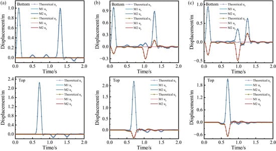
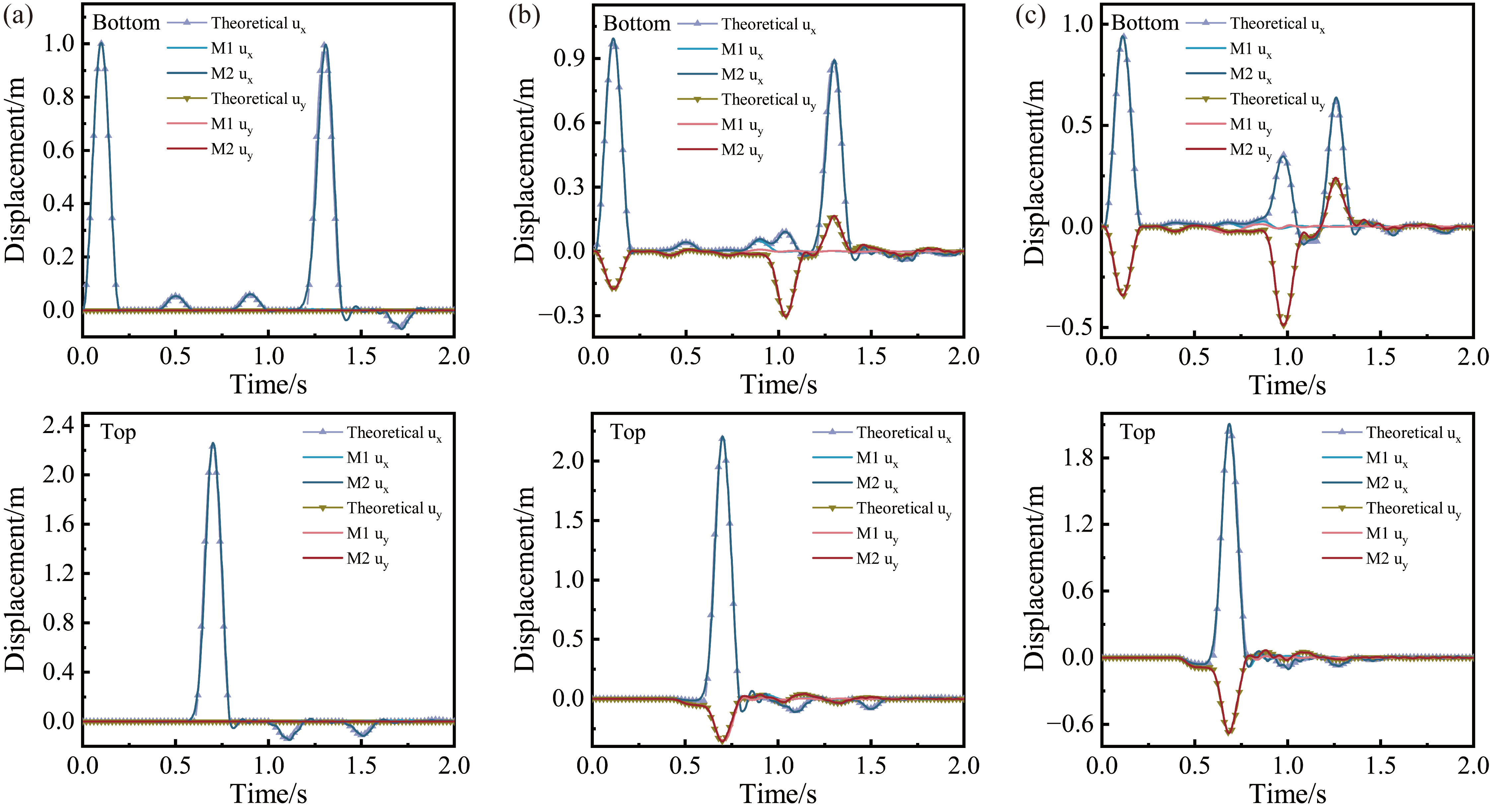
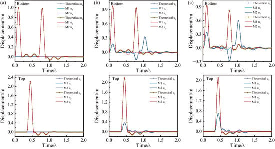
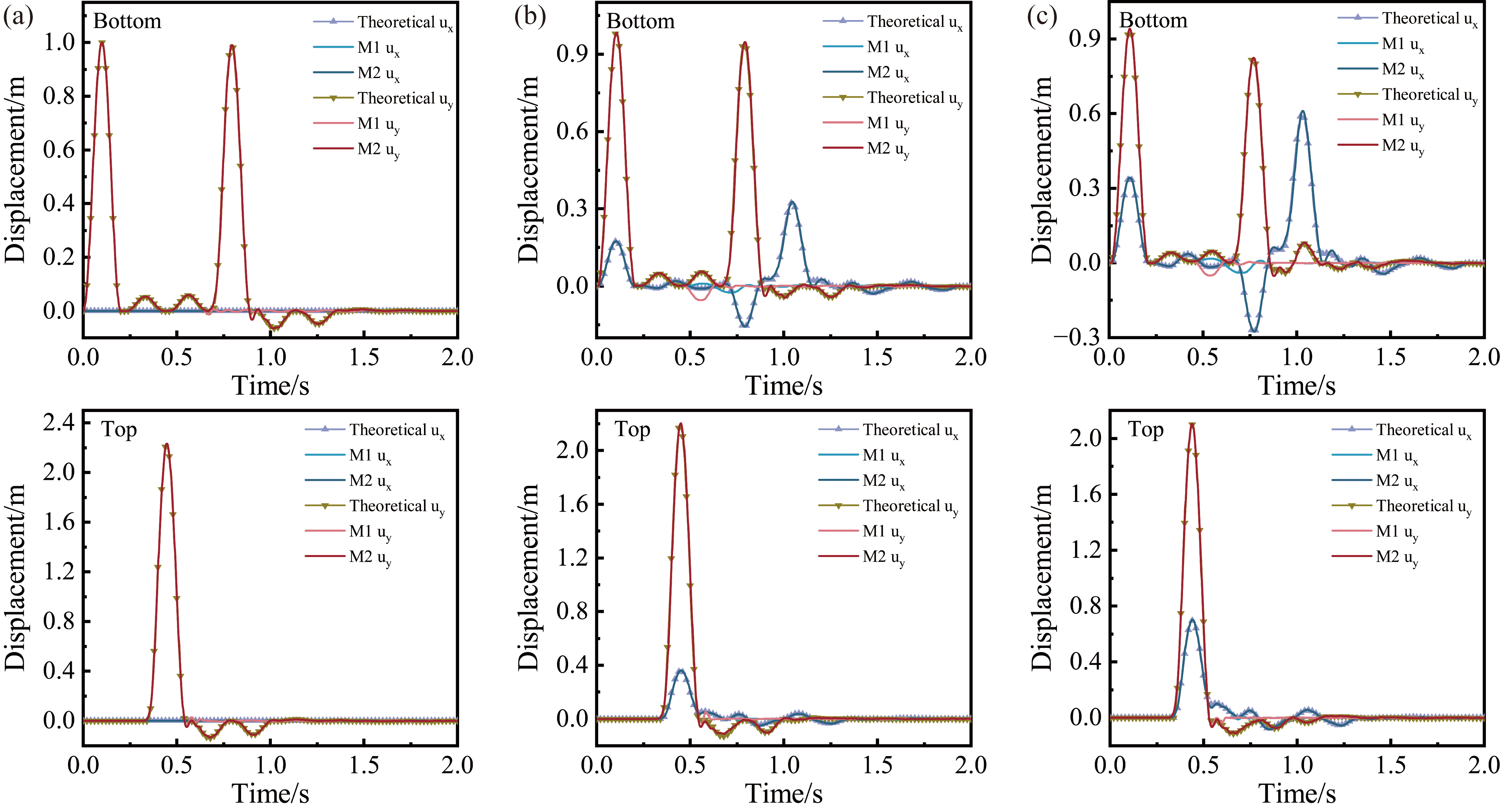
Figure 8 compares the displacement time histories at monitoring point A (top) and monitoring point B (bottom center), as shown in Figure 7, under SV-wave incidence. Method 1 (M1) considers only one reflection and one transmission in each soil layer [20], whereas Method 2 (M2) is the path cumulative amplitude coefficient based method proposed in this study. For incident angles of 0°, 10°, and 20°, the average NRMSE values of M1 are 10.62%, 11.48%, and 10.11%, respectively. These values decrease to 1.91%, 1.65%, and 1.25% for M2. The corresponding Pearson correlation coefficients increase from 0.838, 0.773, and 0.814 to 0.996, 0.997, and 0.998. Overall, M2 reproduces both the amplitude and phase characteristics of the layered soil response with substantially higher accuracy. The superiority of M2 becomes more evident after the first-arrival and initial reflected waves have passed. For the 10° case, the theoretical solution exhibits distinct wave packets at the bottom monitoring point during 0.84–1.09 s and 1.21–1.38 s. These wave packets arise from subsequent reflected and transmitted waves. They are largely absent in the M1 results, whereas M2 accurately reproduces their arrival times, amplitudes, and waveform evolution. This comparison confirms that retaining propagation paths with non-negligible contributions is essential for representing multipath wave superposition in layered soil.

Figure 8. Displacement time histories at the monitoring points under SV wave incidence: (a) 0° incidence; (b) 10° incidence; (c) 20° incidence.

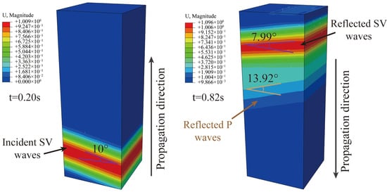
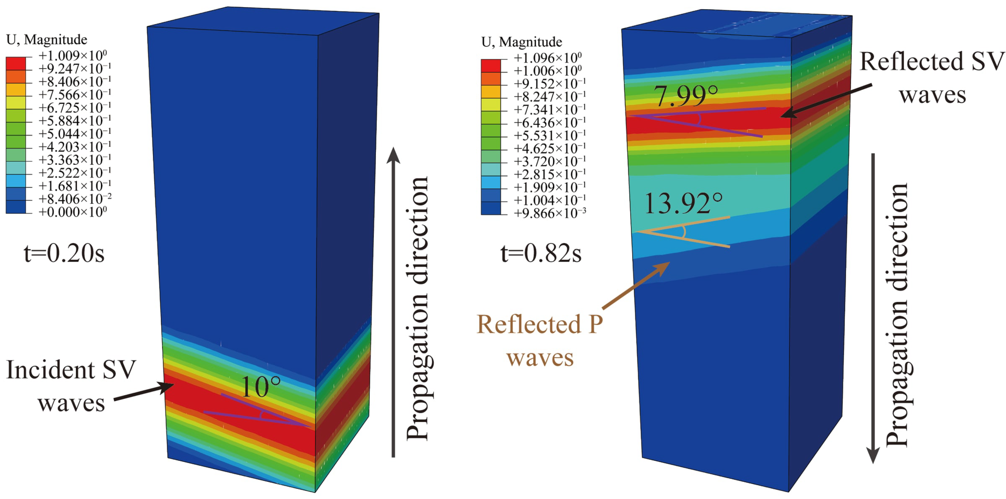
Figure 9 further illustrates SV wave propagation for the 10° incidence case. At t = 0.2 s, only the incident SV wave is present in the finite domain. At 0.82 s, free-surface reflection and mode conversion generate reflected SV and P waves. Their wavefront angles relative to the horizontal plane are 7.99° and 13.92°, respectively. Because the P wave propagates faster, its wavefront travels farther over the same time interval. The propagation sequence and wavefront angles agree well with the theoretical predictions.

Figure 9. Wave propagation snapshots of obliquely incident SV wave in the finite domain.

Figure 10 shows a similar improvement under P wave incidence. For 0°, 10°, and 20°, the average NRMSE values decrease from 10.43%, 11.73%, and 10.95% for M1 to 0.53%, 1.08%, and 0.88% for M2. Meanwhile, the Pearson correlation coefficients increase from 0.837, 0.765, and 0.782 to 0.9997, 0.9988, and 0.9991. A representative discrepancy occurs in the 10° case. At approximately 0.56 s, the theoretical bottom vertical displacement reaches 0.05543 m, and the M2 error is only 1.06%. In contrast, M1 predicts −0.05432 m, indicating a pronounced phase reversal. A similar phenomenon is observed at 20°. These results show that premature truncation of propagation paths can distort both the local amplitude and phase of the response.

Figure 10. Displacement time histories at the monitoring points under P wave incidence: (a) 0° incidence; (b) 10° incidence; (c) 20° incidence.

After the major wave packets pass, the displacement responses at all monitoring points decay smoothly toward zero. No persistent oscillations or spurious reflections are observed. This confirms that the VAB effectively absorbs outgoing waves and reasonably represents the radiation damping of the semi-infinite foundation.

4.2. Seismic Wave Validation

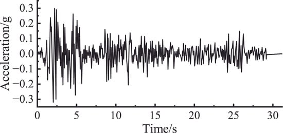
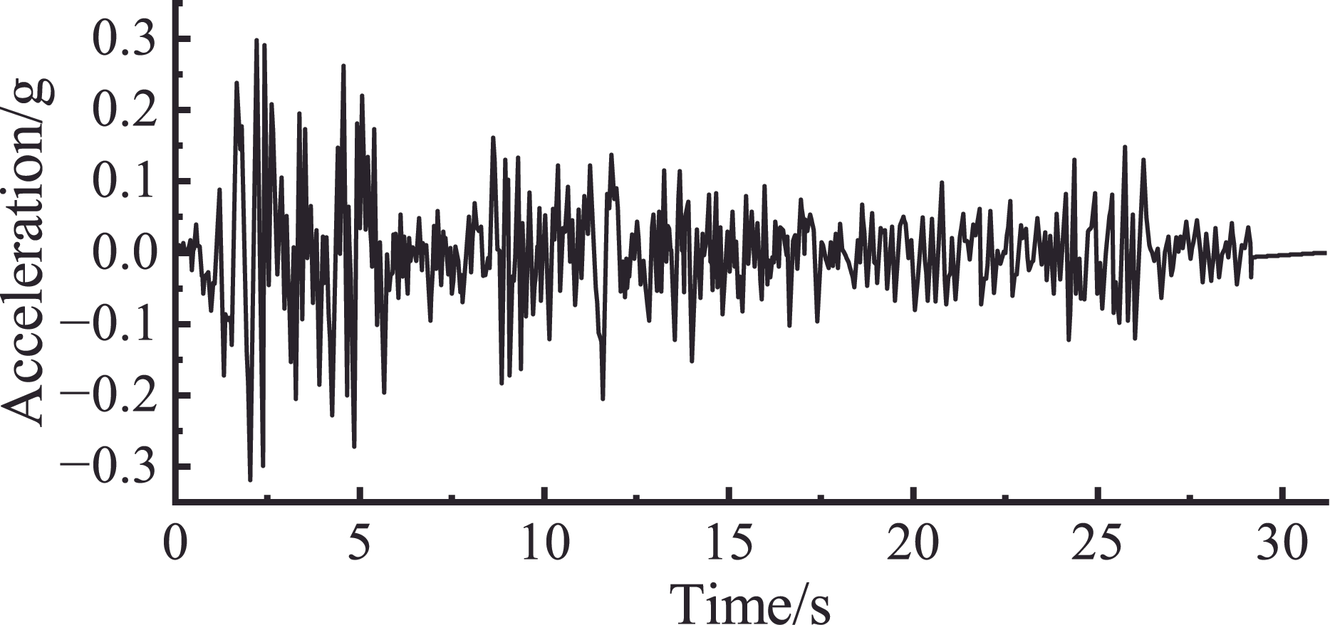
To further verify the applicability and accuracy of the proposed method and assess the effects of the path truncation threshold on response accuracy and computational efficiency, the El Centro earthquake record, baseline-corrected using SeismoSignal, was used to define an SV wave obliquely incident at 20° from the base of the model shown in Figure 7. The truncation threshold ε was set to 0.01, 0.001, and 0.0001 in separate cases. The responses were compared over 0–31.18 s at a sampling interval of 0.02 s, and the total number of retained paths and the input-processing time were recorded for each case. The El Centro acceleration record is shown in Figure 11.

Figure 11. Acceleration time history of the El Centro earthquake record.

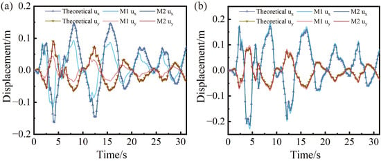
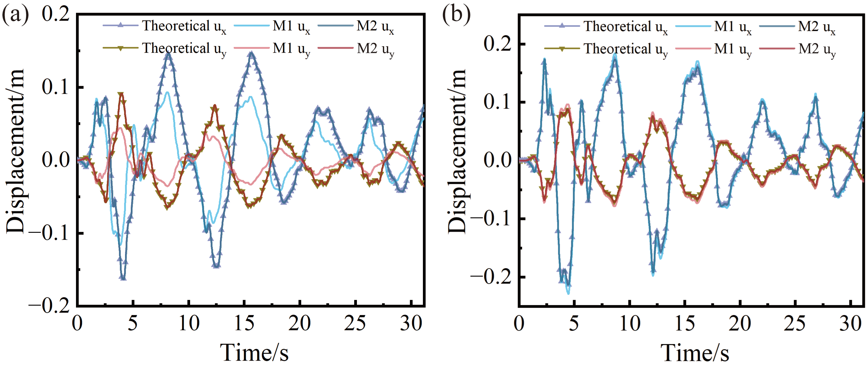
Figure 12 compares the theoretical and numerical displacement time histories under obliquely incident El Centro excitation. The same incident wave, incidence angle, and soil parameters are used for both methods. Compared with the theoretical solution, the peak u_x and u_y displacements predicted by M1 at the top monitoring point are 7.01% and 10.49% larger, respectively. At the bottom monitoring point, however, the corresponding M1 peak values are 28.93% and 52.01% smaller than the theoretical solution. The NRMSE values of M1 for the horizontal and vertical displacement histories are 2.95% and 4.63% at the top midpoint, respectively, increasing to 22.42% and 19.84% at the bottom midpoint. These location-dependent deviations indicate that the response of layered soil is governed by multipath wave superposition involving incident, reflected, transmitted, and mode-converted waves, as well as free-surface reflections, rather than by the first-arriving wave and a limited number of initial reflected and transmitted components. By truncating subsequent propagation paths of waves reflected at layer interfaces, M1 omits wave components that make non-negligible contributions to the response. This weakens the superposition of subsequent wave packets with the main response, limiting the representation of interactions within the multipath wavefield and leading to different deviation patterns at the top and bottom monitoring points. In contrast, M2 retains higher-order reflected and transmitted components that make non-negligible contributions to the response through the path cumulative amplitude coefficient and therefore better represents propagation delay, amplitude variation, phase difference, and multipath superposition.

Figure 12. Displacement time histories at the monitoring points under El Centro earthquake excitation: (a) bottom center; (b) top center.

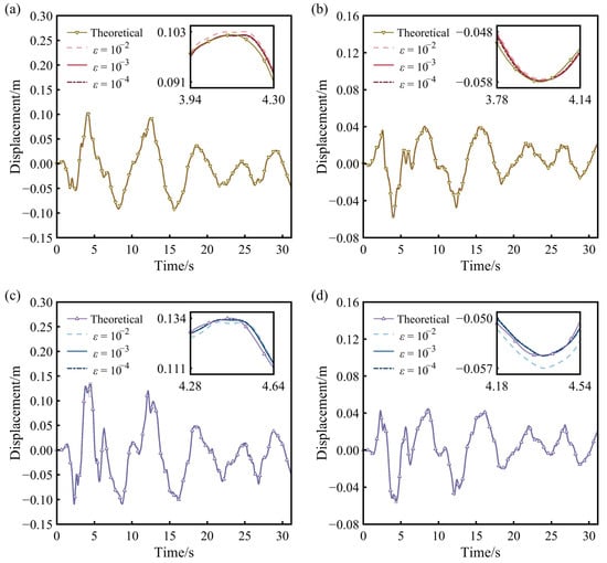
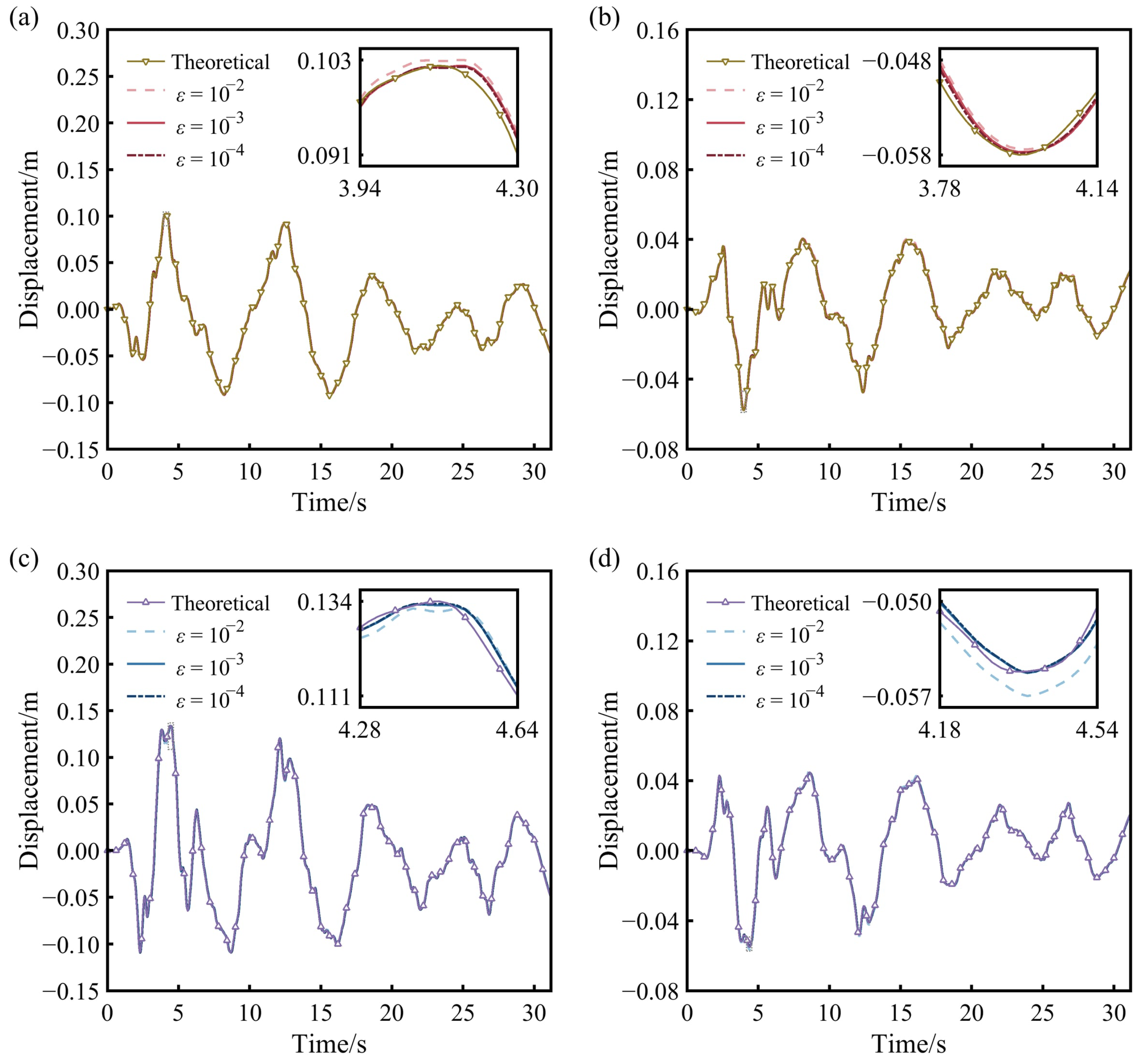
The numerical results obtained using M2 agree closely with the theoretical solutions over the entire time history. By incorporating these additional propagation contributions, M2 reproduces the main peaks and troughs, phase characteristics, and waveform variations of the theoretical response. At ε = 0.001, the relative errors of the peak u_x and u_y responses are 0.02% and −0.61% at the bottom monitoring point and −0.50% and 0.43% at the top monitoring point, respectively. The NRMSE values are approximately 1%, while all Pearson correlation coefficients exceed 0.9994. These results confirm that the proposed method accurately reproduces both peak responses and waveform evolution, with good phase alignment over the entire time history.

Figure 13 further compares the displacement time histories obtained using different truncation thresholds. Enlarged views around the main peaks of each displacement component highlight the response differences caused by threshold variations. When ε decreases from 0.01 to 0.001, the mean NRMSE decreases from 1.66% to 1.08%, representing a reduction of 34.94%. The maximum NRMSE among displacement components decreases from 1.96% to 1.14%, the maximum absolute relative error in peak displacement decreases from 3.32% to 0.61%, and the minimum Pearson correlation coefficient increases from 0.9989 to 0.9995. Further reducing ε to 0.0001 gives a mean NRMSE of 0.99%, a maximum NRMSE among displacement components of 1.13%, a maximum absolute relative error in peak displacement of 0.45%, and a minimum Pearson correlation coefficient of 0.9996. Compared with ε = 0.001, the mean NRMSE decreases by only a further 0.09 percentage points and the maximum NRMSE among displacement components by 0.01 percentage points. The results for both thresholds agree closely with the theoretical waveforms. The overall error decreases as the threshold is reduced, while the accuracy gain from 0.001 to 0.0001 becomes markedly smaller, indicating a clear trend toward convergence in the numerical response. At ε = 0.001, the principal propagation components governing the overall response are already adequately retained.

Figure 13. Displacement time histories at the monitoring points for different truncation thresholds: (a) horizontal displacement at the bottom midpoint; (b) vertical displacement at the bottom midpoint; (c) horizontal displacement at the top midpoint; (d) vertical displacement at the top midpoint.

In path tracing, increasing the number of soil interfaces with impedance contrasts increases the potential combinations of reflection, transmission, and mode conversion paths. Lowering the threshold retains more low-amplitude paths, increasing the computational effort required for path tracing, time-history superposition, and boundary load generation. Screening based on cumulative amplitude ratios concentrates input-processing resources on propagation components with larger contributions to the response. Table 2 illustrates the method’s ability to balance accuracy and computational cost. M1 retains 21 paths, and its input-processing time is normalized to 1.00. At ε = 0.01, 0.001, and 0.0001, M2 retains 90, 203, and 880 paths, respectively, with corresponding normalized input-processing times of 1.85, 2.91, and 10.72. At ε = 0.001, M2 achieves a mean NRMSE of approximately 1%, a maximum absolute relative error in peak displacement below 1%, and Pearson correlation coefficients above 0.9994 through a moderate increase in the number of retained paths. M2 thus improves response accuracy over M1 while keeping the input-processing cost manageable. When ε is further reduced from 0.001 to 0.0001, the number of retained paths and the input-processing time increase to 4.33 and 3.68 times their previous values, respectively, while the mean NRMSE decreases by only a further 0.10 percentage points. Compared with ε = 0.0001, using ε = 0.001 reduces the number of retained paths by 76.93% and the input-processing time by 72.85%, while maintaining comparable accuracy in reproducing both the full response time histories and peak displacements.

Table 2. Comparison of errors and computational cost for M1 and M2 with different truncation thresholds.

Method	Truncation Threshold	Mean NRMSE (%)	Maximum Absolute Relative Error in Peak Displacement (%)	Minimum Pearson Correlation Coefficient	Total Number of Retained Paths	Normalized Input-Processing Time
M1	-	12.46	52.01	0.8655	21	1.00
M2	0.01	1.66	3.32	0.9989	90	1.85
M2	0.001	1.08	0.61	0.9995	203	2.91
M2	0.0001	0.99	0.45	0.9996	880	10.72

5. Engineering Application to the Pingyao Ancient City Wall

5.1. Numerical Model and Seismic Input

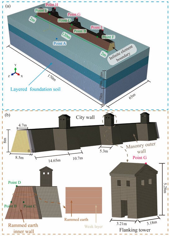
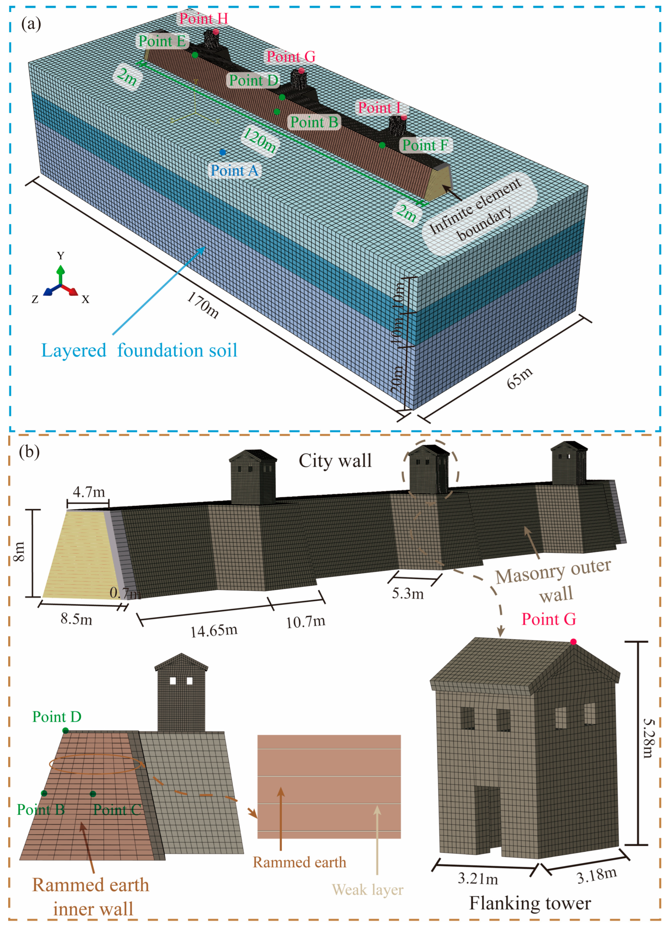
The seismic performance assessment of earthen heritage sites has long been a major focus in the fields of cultural heritage conservation and disaster mitigation [37,38]. In this study, the Pingyao Ancient City Wall, a UNESCO World Heritage Site in Shanxi Province, China, was selected for seismic response analysis. The wall consists of a rammed earth core constructed by layer-by-layer compaction of local loess, with exterior brick facing and brick flanking towers along the crest.

A typical wall segment was modeled, as shown in Figure 14. The masonry of the flanking towers and exterior facing was described using the concrete damage plasticity model (CDP) within a homogenized modeling approach to represent its nonlinear behavior, with a density of 1800 kg/m³, elastic modulus of 1341.4 MPa, Poisson’s ratio of 0.15, compressive strength of 2.36 MPa, and tensile strength of 0.157 MPa. The tensile softening and damage evolution relationships followed the forms adopted in Refs. [34,39].

Figure 14. Finite element model of the Pingyao Ancient City Wall: (a) overall model of the city wall-soil system; (b) geometry and construction details of the city wall and flanking towers.

To represent the layered construction of the rammed earth core, the wall was divided into 25 compacted layers using the element activation-deactivation technique. A 10 mm weak interface was inserted between adjacent layers [40]. The rammed earth and weak interface layers were modeled using the modified Mohr–Coulomb constitutive model [41], with material parameters listed in Table 3 and a tensile strength adjustment coefficient of 0.05. Hard contact was adopted in the normal direction, and Coulomb friction with a coefficient of 0.7 was used in the tangential direction at both the flanking tower-wall and brick facing-rammed earth interfaces. Infinite elements were assigned to the two longitudinal ends of the wall to approximate its extended longitudinal continuity [42].

Table 3. Physical and mechanical properties of the rammed earth wall.

	Young’s Modulus E/MPa	Poisson’s Ratio v	Cohesion c/kPa	Internal Friction Angle φ/°	Lode Angle θT/°
Rammed earth	100.8	0.30	178.0	30.1	25
Weak layer	85.7	0.30	151.3	26.2	25

Based on the site investigation, the foundation was modeled as a 170 m × 65 m × 40 m three-layer system [9,34]. From top to bottom, the soil profile consists of a 10 m silt layer (ρ = 1.82 g/cm³, c_s = 210.3 m/s, v = 0.31), a 10 m silty clay layer (ρ = 1.85 g/cm³, c_s = 239.7 m/s, v = 0.30), and a 20 m silt layer (ρ = 1.87 g/cm³, c_s = 266.4 m/s, v = 0.28). A geostatic analysis was first performed to establish the initial stress state, after which the boundary conditions were converted for dynamic analysis [43,44].

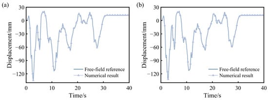
Considering the seismic fortification intensity of 8 in the Pingyao region and the Class III site conditions adopted in this study, the El Centro record was adopted as a reference waveform for constructing the incident SV wave and scaled to a reference peak acceleration of 0.20 g. In a homogeneous elastic half-space, a vertically incident shear wave and its reflected wave superpose in phase with equal amplitudes at a flat free surface, so that the outcrop motion amplitude is twice that of the upgoing incident wave [45]. Following this amplitude relationship and the input settings adopted in previous studies [32,46,47], the amplitude of the scaled record was reduced by half to construct the upgoing incident SV wave at the site base. This factor of one-half specifies the incident excitation intensity. Impedance contrasts, wave reflection and transmission, P-SV mode conversion, and propagation delays in the actual layered site are explicitly accounted for by the proposed method. Motions at the ground surface and within the soil are obtained through the corresponding free field analysis, and the resulting free field response is converted into equivalent nodal loads on the viscoelastic artificial boundaries to implement the seismic input. To examine the influence of incidence angle on the wall’s dynamic response, both vertical incidence and 10° oblique incidence were considered. The incidence angle was measured from the vertical, and the plane of incidence was defined by the longitudinal and vertical directions of the wall. The horizontal particle-motion component was oriented along the longitudinal direction of the city wall (the X-direction).

5.2. Seismic Response and Damage Analysis

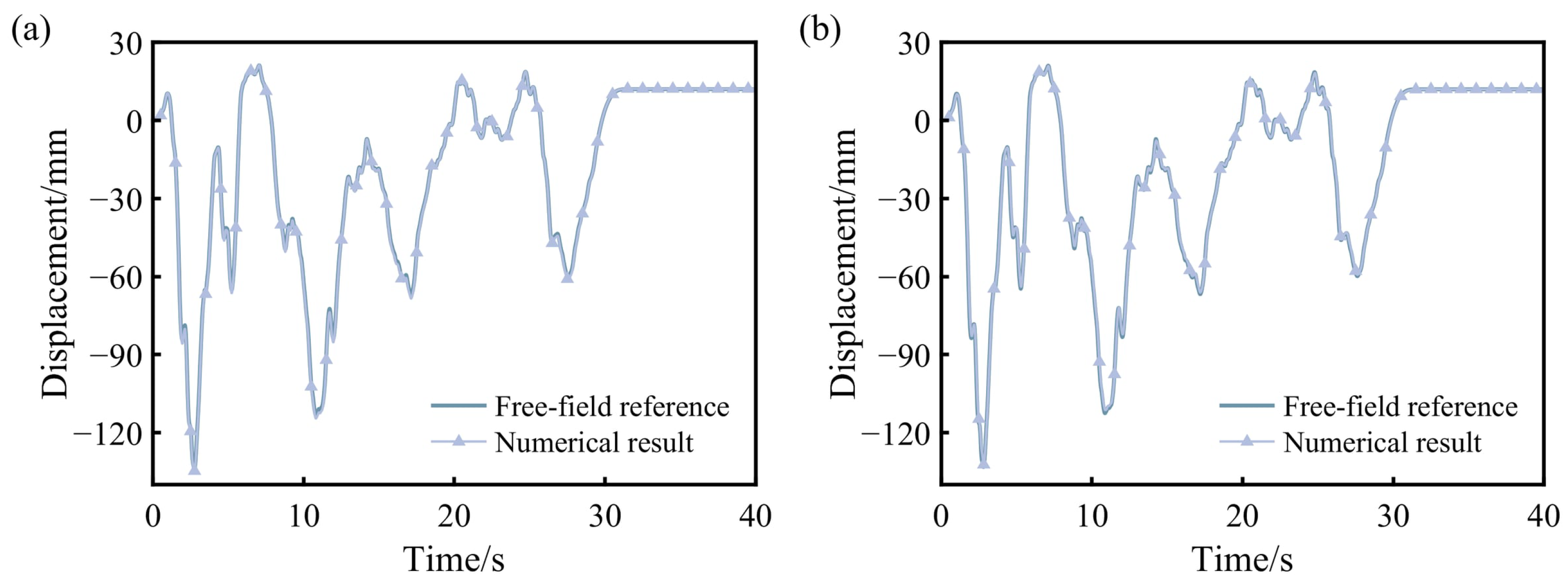
Figure 15 compares the numerical and theoretical horizontal displacement time histories at ground Point A. Before the incident wave arrives, the numerical response remains nearly zero, indicating that the VAB and ENF input scheme introduces no noticeable initial disturbance. The proposed method yields peak relative errors of 0.52% and 0.70% for vertical and 10° oblique incidence, respectively. The corresponding NRMSE values are 0.47% and 0.60%, and the Pearson correlation coefficients are at least 0.9996 in both cases. In both cases, the numerical response accurately reproduces the major peaks, troughs, and phase characteristics throughout the time history. As the excitation decays, the response converges smoothly without numerical divergence, following the same trend as the theoretical solution. These results confirm that the proposed method can still accurately reproduce the free-field response of layered soil in the SSI model.

Figure 15. Comparison of horizontal displacement time histories at Point A: (a) vertical incidence; (b) 10° oblique incidence.

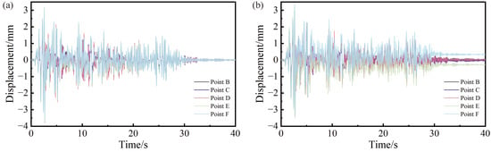
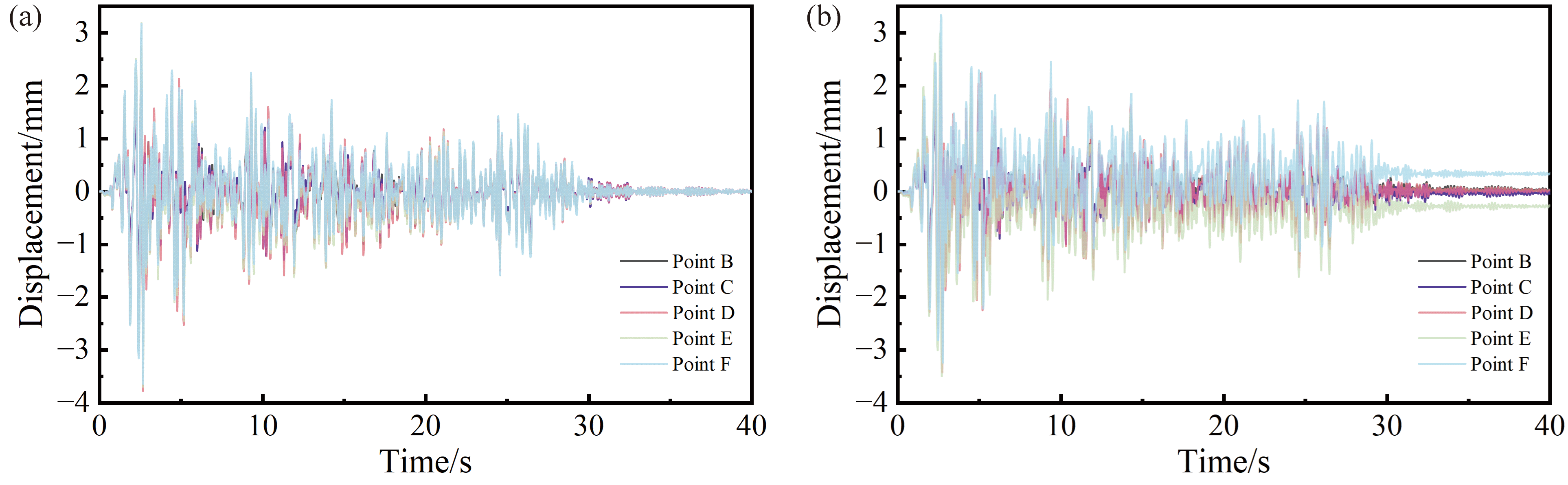
Figure 16 presents the horizontal displacement time histories at representative points along the city wall. Point E is located on the incident-wave side, whereas Point F is on the back-wave side. Point D is located in the upper part of the central wall segment. Compared with vertical incidence, 10° oblique incidence reduces the peak absolute displacements at Points E, D, and F by 5.49%, 9.45%, and 8.24%, respectively, indicating that the effect of incidence angle on response amplitude varies with location. Under vertical incidence, the positive and negative peaks at Points E, D, and F occur at 2.56 s and 2.66 s, respectively, indicating nearly synchronous major peaks. Under 10° oblique incidence, the peak responses occur at different times. The positive peaks appear at 2.60, 2.62, and 2.64 s at Points E, D, and F, respectively, while the corresponding negative peaks occur at 2.70, 2.72, and 2.76 s. These progressive time shifts indicate that the wall does not respond synchronously under obliquely incident SV waves. Instead, propagation delay produces evident phase lags and spatially non-uniform seismic responses along the longitudinal direction. The peak absolute displacements at Points D, E, and F under 10° oblique incidence are of the same order of magnitude, indicating no abrupt amplification along the wall. However, the peak-to-peak displacement at the back-wave-side Point F is slightly larger than that at Point E. This suggests a greater cyclic displacement range on the back-wave side. The difference reflects the combined effects of propagation delay, superposition with the structural inertial response, and local scattering: when the seismic motion reaches the back-wave side, it interacts with the inertia-induced response that has already developed in the incident-wave-side and central wall segments and with locally scattered waves in the wall, producing more pronounced cyclic deformation in the back-wave-side wall segment. As a result, the later arrival of the wave does not necessarily lead to a smaller response, and larger displacement responses may develop under these combined effects.

Figure 16. Displacement time histories at the monitoring points of the city wall: (a) vertical incidence; (b) 10° oblique incidence.

The displacement amplitude at the slope-surface Point B is larger than that at the interior Point C under both incidence conditions, indicating a surface amplification effect associated with weaker confinement near the exposed slope surface. In addition, the response at the upper Point D exceeds that at Point B, showing a clear elevation amplification effect. The reduced lateral restraint near the wall crest contributes to this increase. After the main excitation, the displacement responses gradually approach stable values without persistent oscillations or numerical divergence. Residual displacements remain at several points, indicating irreversible deformation of the rammed earth wall.

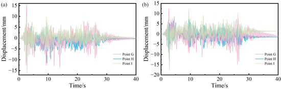
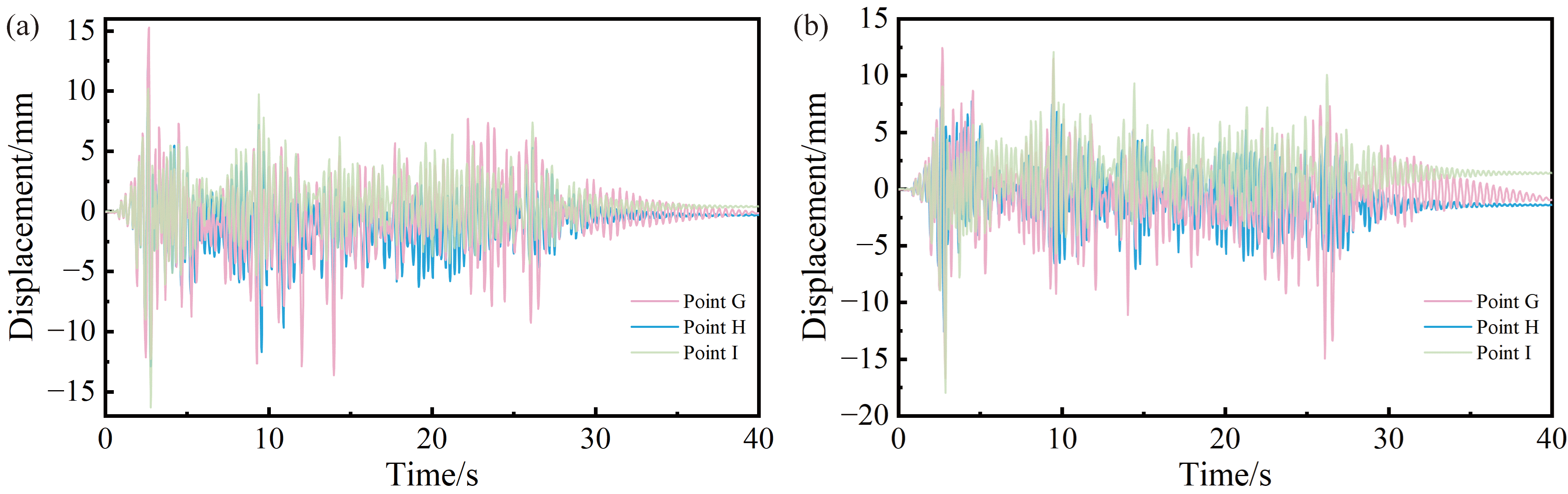
Figure 17 presents the horizontal displacement time histories at the tops of the flanking towers under vertical and 10° oblique incidence. Compared with vertical incidence, 10° oblique incidence reduces the peak absolute displacement at the incident-wave-side Point H by 5.03%, whereas those at the central Point G and the back-wave-side Point I increase by 9.11% and 10.31%, respectively. These changes indicate that the effect of incidence angle differs considerably among towers at different locations. Under both conditions, the displacement response is largest at the back-wave-side tower, followed by the central and incident-wave-side towers. Oblique incidence further increases the displacement responses of the central and back-wave-side towers. Compared with vertical incidence, the peak-to-peak displacement under 10° oblique incidence decreases by 22.21% at Point H and increases by 0.75% and 13.42% at Points G and I, respectively. Thus, the back-wave-side tower experiences both a larger peak absolute displacement and greater cyclic displacement range under 10° oblique incidence. Further comparisons between towers show that, under vertical incidence, the peak absolute and peak-to-peak displacements at Point I exceed those at Point H by 22.96% and 1.46%, respectively. Under 10° oblique incidence, the peak absolute displacement at Point I is 42.82% greater than that at Point H, while the peak-to-peak displacement is 47.92% larger. Similarly, the percentage by which the peak absolute displacement at Point G exceeds that at Point H increases from 15.37% under vertical incidence to 32.54% under 10° oblique incidence. These results indicate that oblique incidence changes the response amplitudes of individual towers and further increases the spatial differences between the incident-wave-side tower and the central and back-wave-side towers, making the stronger responses of the latter two towers more pronounced.

Figure 17. Displacement time histories at the monitoring points of the flanking towers: (a) vertical incidence; (b) 10° oblique incidence.

The flanking towers also exhibit spatially varying torsional responses. Under vertical incidence, the peak torsional angles of the incident-wave-side, central, and back-wave-side towers are 0.0017, 0.0085, and 0.0017, respectively. The central tower’s peak torsional angle is five times that of either side tower. Under 10° oblique incidence, the peak torsional angles of the incident-wave-side, central, and back-wave-side towers are 0.0011, 0.0244, and 0.0055, respectively. Compared with vertical incidence, the peak torsional angle decreases by 35.29% at the incident-wave-side tower and increases by 187.06% and 223.53% at the central and back-wave-side towers, respectively. The central tower’s peak is 22.18 and 4.44 times those of the incident-wave-side and back-wave-side towers, respectively. Under oblique incidence, the central tower accommodates the non-synchronous deformation of adjacent wall segments through local rotation about the vertical axis. This produces asymmetric forces on the two sides of its base, increasing local damage. The percentage increase in the central tower’s peak torsional angle is much greater than the 9.11% increase in its peak absolute horizontal displacement. The back-wave-side tower exhibits increases in both horizontal displacement and torsional response.

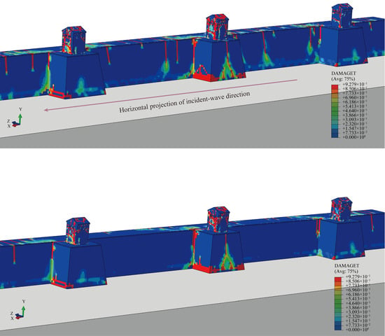
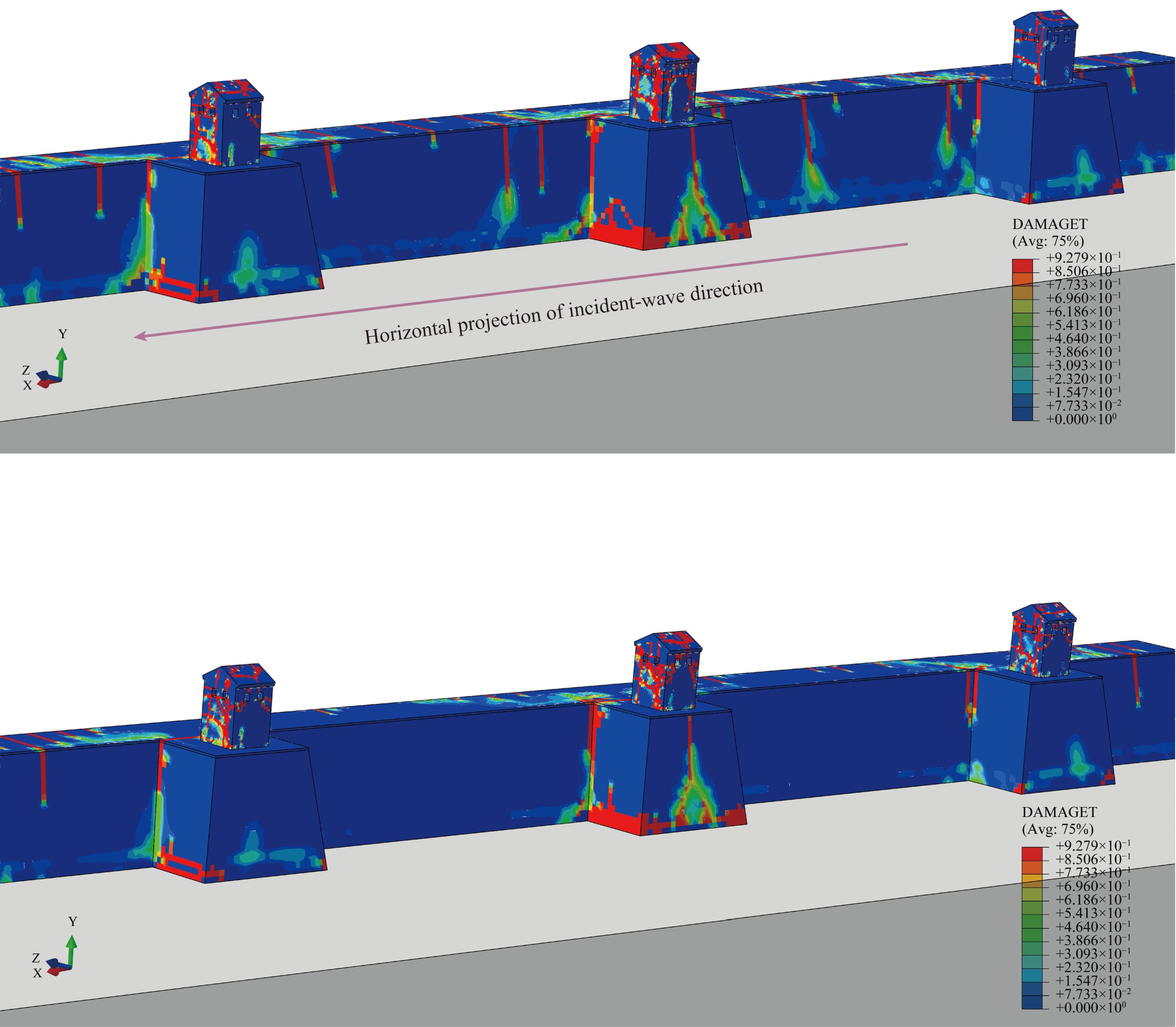
Figure 18 presents the tensile damage distributions in the city wall under the two incidence conditions. Tensile damage in the masonry is represented by the DAMAGET variable in the CDP model. A value of zero indicates no tensile damage, and larger values indicate greater tensile stiffness degradation. Under vertical incidence, the overall tensile damage distributions are similar among the three flanking towers. Under 10° oblique incidence, the incident-wave-side tower exhibits a noticeably smaller damaged region, whereas the back-wave-side tower shows more pronounced local damage and a more continuous damage distribution. The central tower exhibits relatively concentrated local damage. The damage distributions correspond well to the displacement and torsional responses. The reduced displacement and torsional responses of the incident-wave-side tower correspond to less tensile damage. The increased horizontal cyclic deformation and torsional response of the back-wave-side tower correspond to the development of local damage, while the concentrated tensile damage in the central tower is consistent with its pronounced local torsional response.

Figure 18. Tensile damage contours of the flanking towers: (a) vertical incidence; (b) 10° oblique incidence.

As the excitation subsides, the displacement amplitudes of the flanking towers generally decay, and their responses gradually stabilize, with numerical stability maintained throughout the dynamic analysis. Compared with vertical incidence, 10° oblique incidence produces larger post-earthquake residual displacements in all three flanking towers, further demonstrating the influence of incidence angle on the post-earthquake displacement distribution.

The Pingyao Ancient City Wall case links the proposed method to the seismic response assessment of long, linear heritage structures. For city walls with flanking towers distributed along their length and local variations in structural configuration, assessments should consider overall displacement, the response timing of different wall segments, torsional responses of the flanking towers, and local damage distributions. These analyses can inform the selection of locations for focused inspection, the placement of monitoring points, and comparisons of local strengthening schemes. In engineering applications, model and input parameters should be determined based on site investigations and the existing condition of the structure, and assessments should integrate analysis results from multiple ground motion scenarios.

6. Conclusions

A seismic input method for layered foundations was developed within the VAB framework using the path cumulative amplitude coefficient for propagation-path selection and truncation. The method retains a single reflection at each interface and the corresponding induced transmitted waves, and accounts for propagation delay, amplitude variation, spatial phase difference, and mode conversion under oblique incidence. The main conclusions are as follows:

(1) The proposed method provides a unified formulation for vertically and obliquely incident P and S waves in layered soil. Compared with the simplified method that considers only one reflection and one transmission in each layer, it retains wave components with non-negligible contributions and more accurately represents multipath superposition. This reduces amplitude errors and phase distortion caused by premature path truncation.

(2) Harmonic wave validation confirms the accuracy of the proposed method. For SV wave incidence at 0°, 10°, and 20°, the average NRMSE ranges from 1.25% to 1.91%, with Pearson correlation coefficients above 0.996. For P wave incidence, the corresponding NRMSE ranges from 0.53% to 1.08%, and the correlation coefficients exceed 0.998. The propagation sequence and wavefront angles also agree well with the theoretical solutions.

(3) Under obliquely incident El Centro excitation, the method reproduces theoretical displacement responses with a mean NRMSE of 1.08% and absolute relative errors in peak displacement no greater than 0.61% at a truncation threshold of 0.001. Within the investigated range, responses tend to converge as the threshold decreases, with more retained paths, longer input-processing times, and diminishing accuracy gains. Selection based on the path cumulative amplitude coefficient enables a balance between response accuracy and input-processing cost.

(4) The Pingyao Ancient City Wall case demonstrates the method’s application in SSI analysis. With the same structural model and prescribed incident SV wave intensity, 10° oblique incidence progressively delays major response peaks along the wall compared with vertical incidence. It reduces peak absolute displacement and tensile damage in the incident-wave-side tower but increases displacement and torsional responses in the central and back-wave-side towers, altering local damage distributions. These changes indicate that analyses assuming spatially uniform ground motion alone may not accurately identify critical locations.

The free field input formulation in this study assumes horizontal layering, perfectly bonded interfaces, and linear wave propagation, with oblique incidence restricted to subcritical angles. For minor earthquakes and moderate earthquakes with limited soil strains, linear or strain-compatible equivalent-linear site models have an established basis in engineering practice and can be coupled with nonlinear structural and contact analyses in the near field. However, when strong shaking induces significant soil nonlinearity, modulus degradation, cyclic plasticity, and interlayer slip or opening cause wave propagation characteristics to evolve with the loading history. These processes are difficult to capture fully using the current path superposition method with fixed coefficients. The superposition formulation based on real propagation angles and travel times also requires extension to account for evanescent components under supercritical incidence. Future work could integrate iterative strain-compatible parameter updates and nonlinear time-domain free-field solvers with the path-based input framework to maintain consistency among wave propagation, dissipation, and boundary treatment. The spatial decay and phase descriptions of evanescent components could also be improved to extend applicability to supercritical incidence. For inclined or irregular interfaces and laterally heterogeneous sites, path tracing based on local interface normals could be combined with two- or three-dimensional free-field solutions to account for mode conversion, focusing, diffraction, and lateral scattering in complex sites.

References

- Ceroni, F.; Sica, S.; Pecce, M.R.; Garofano, A. Evaluation of the natural vibration frequencies of a historical masonry building accounting for SSI. Soil Dyn. Earthq. Eng. 2014, 64, 95–101. [Google Scholar] [CrossRef] [Scilit]
- Lazizi, A.H.; Tahghighi, H. Influence of Soil–Structure Interaction on Seismic Demands of Historic Masonry Structure of Kashan Grand Bazaar. Bull. Earthq. Eng. 2023, 21, 151–176. [Google Scholar] [CrossRef] [Scilit]
- Wang, J.; Guo, T.; Du, Z.; Yu, S. Shaking Table Tests and Parametric Analysis of Dynamic Interaction between Soft Soil and Structure Group. Eng. Struct. 2022, 256, 114041. [Google Scholar] [CrossRef] [Scilit]
- Wang, J.; Guo, T.; Xie, Y.; Du, Z. Parametric Analyses of Dynamic Interaction between Three-Dimensional Soil and Frame Structure Group under Earthquake Loadings. Bull. Earthq. Eng. 2022, 20, 8305–8324. [Google Scholar] [CrossRef] [Scilit]
- Lysmer, J.; Kuhlemeyer, R.L. Finite Dynamic Model for Infinite Media. J. Eng. Mech. Div. 1969, 95, 859–877. [Google Scholar] [CrossRef] [Scilit]
- Xing, H.; Li, X.; Li, H.; Liu, A. Spectral-Element Formulation of Multi-Transmitting Formula and Its Accuracy and Stability in 1D and 2D Seismic Wave Modeling. Soil Dyn. Earthq. Eng. 2021, 140, 106218. [Google Scholar] [CrossRef] [Scilit]
- Saleh Asheghabadi, M.; Ali, Z. Infinite Element Boundary Conditions for Dynamic Models under Seismic Loading. Indian J. Phys. 2020, 94, 907–917. [Google Scholar] [CrossRef] [Scilit]
- Shabani, A.; Feyzabadi, M.; Kioumarsi, M. Model Updating of a Masonry Tower Based on Operational Modal Analysis: The Role of Soil-Structure Interaction. Case Stud. Constr. Mater. 2022, 16, e00957. [Google Scholar] [CrossRef] [Scilit]
- Özmen, A.; Sayin, E. Different Soil-Structure Interaction Modelling Strategies for Seismic Analysis of a Masonry Church. Int. J. Archit. Herit. 2025, 19, 1341–1361. [Google Scholar] [CrossRef] [Scilit]
- Deeks, A.J.; Randolph, M.F. Axisymmetric Time-domain Transmitting Boundaries. J. Eng. Mech. 1994, 120, 25–42. [Google Scholar] [CrossRef] [Scilit]
- Liu, J.; Du, Y.; Du, X.; Wang, Z.; Wu, J. 3D Viscous-Spring Artificial Boundary in Time Domain. Earthq. Engin. Engin. Vib. 2006, 5, 93–102. [Google Scholar] [CrossRef] [Scilit]
- Bao, X.; Liu, J.-B.; Li, S.-T.; Wang, F. A New Viscoelastic Artificial Boundary with Improved Numerical Stability in Explicit Calculation of Wave Propagation Problems in Infinite Domains. Comput. Geotech. 2022, 145, 104698. [Google Scholar] [CrossRef] [Scilit]
- Xu, C.; Liu, Q.; Xie, W.; Wang, Y.; Li, S.; Lu, W.; Zhang, H. Investigation on Artificial Boundary Problem in the Combined Finite-Discrete Element Method (FDEM). Comput. Geotech. 2022, 151, 104969. [Google Scholar] [CrossRef] [Scilit]
- Lin, S.; Deng, T.; Zheng, L.; Zhang, H.; Wu, W.; Fu, X.; Chen, G. Implementation of Viscoelastic Artificial Boundary and Seismic Motion Input Method in Three-Dimensional Discontinuous Deformation Analysis Method. Rock Mech. Rock Eng. 2024, 57, 4995–5015. [Google Scholar] [CrossRef] [Scilit]
- Li, Y.; Zhao, M.; Xu, C.; Du, X.; Li, Z. Earthquake Input for Finite Element Analysis of Soil-Structure Interaction on Rigid Bedrock. Tunn. Undergr. Space Technol. 2018, 79, 250–262. [Google Scholar] [CrossRef] [Scilit]
- Li, X.; He, Q.; Ling, K.; Wu, H.; Wang, J.; Liu, D. Seismic Response of Masonry Pagodas Considering Soil-Structure-Interaction (SSI) Effect and CFRP Reinforcement. npj Herit. Sci. 2025, 13, 49. [Google Scholar] [CrossRef] [Scilit]
- Chen, D.; Hou, C.; Wang, F. Influences on the Seismic Response of the Gravity Dam-Foundation-Reservoir System with Different Boundary and Input Models. Shock Vib. 2021, 2021, 6660145. [Google Scholar] [CrossRef] [Scilit]
- Yin, G.; Zhao, L.; Li, T. Viscoelastic artificial boundary model considering layered foundation. Adv. Sci. Technol. Water Resour. 2019, 39, 87–94. (In Chinese) [Google Scholar] [CrossRef]
- Bi, Z.; Cui, B.; Zhai, Y. Research on Seismic Input Method of Layered Ground Foundation. IEEE Access 2021, 9, 54820–54830. [Google Scholar] [CrossRef] [Scilit]
- An, Y.; Chen, X.; Qin, J.; Wang, X.; He, B.; Wang, X.; Ren, Y.; Bai, Z.; Han, P. Seismic Damage Patterns of the Wenfeng Pagoda Considering SSI in a Rammed Earth Foundation via an Improved Wave Method. Bull. Earthq. Eng. 2026, 24, 5777–5810. [Google Scholar] [CrossRef] [Scilit]
- Zhai, Y.; Song, Z.; Liu, Y.; Gao, T.; Bai, Z.; Bi, Z. A New Seismic Input Method for Layered Soil and Its Application in Dynamic Response Analysis of Underground Structure. Structures 2023, 58, 105488. [Google Scholar] [CrossRef] [Scilit]
- Zhou, P.; Cao, G.; Ding, X.; Xu, C.; Zheng, C. Seismic Input Method for Layered Soils in Static-Dynamic Coupling Analyses Based on Infinite Element Boundaries. Soil Dyn. Earthq. Eng. 2026, 203, 110099. [Google Scholar] [CrossRef] [Scilit]
- Gao, Z.; Zhao, M.; Huang, J.; Du, X.; Wu, L. Three-Dimensional Nonlinear Seismic Response Analysis of Subway Station Crossing Longitudinally Inhomogeneous Geology under Obliquely Incident P Waves. Eng. Geol. 2021, 293, 106341. [Google Scholar] [CrossRef] [Scilit]
- Huang, J.-Q.; Du, X.-L.; Jin, L.; Zhao, M. Impact of Incident Angles of P Waves on the Dynamic Responses of Long Lined Tunnels. Earthq. Eng. Struct. Dyn. 2016, 45, 2435–2454. [Google Scholar] [CrossRef] [Scilit]
- Huang, J.; Du, X.; Zhao, M.; Zhao, X. Impact of Incident Angles of Earthquake Shear (S) Waves on 3-D Non-Linear Seismic Responses of Long Lined Tunnels. Eng. Geol. 2017, 222, 168–185. [Google Scholar] [CrossRef] [Scilit]
- Lyu, D.; Ma, S.; Yu, C.; Liu, C.; Wang, X.; Yang, B.; Xiao, M. Effects of Oblique Incidence of SV Waves on Nonlinear Seismic Response of a Lined Arched Tunnel. Shock Vib. 2020, 2020, 8093804. [Google Scholar] [CrossRef] [Scilit]
- Zhang, T.; Xu, Q.; Chen, J.; Li, J. Nonlinear Seismic Response and Index Correlation of High Arch Dams under Cross-Stream Oblique Incidence of near-Fault SV Waves Based on Wavelet Decomposition. Soil Dyn. Earthq. Eng. 2023, 164, 107635. [Google Scholar] [CrossRef] [Scilit]
- Bi, Z.; Zhang, L.; He, X.; Zhai, Y. Effect of Oblique Incidence Angle and Frequency Content of P and SV Waves on the Dynamic Behavior of Liquid Tanks. Soil Dyn. Earthq. Eng. 2023, 171, 107929. [Google Scholar] [CrossRef] [Scilit]
- Wang, F.; Tulamaiti, Y.; Fang, H.; Yu, X.; Zhou, C. Seismic Response Characteristics of Polymer Anti-Seepage Wall in Earth Dam Based on Earthquake Wave Motion Input Method. Structures 2023, 47, 358–373. [Google Scholar] [CrossRef] [Scilit]
- Wang, F.; Song, Z.; Liu, Y.; Luo, B. Seismic Wave Input Method for High Earth Dams Considering the Transmission Amplification Effect of the Bedrock–Overburden Interface. Comput. Geotech. 2021, 130, 103927. [Google Scholar] [CrossRef] [Scilit]
- Wang, F.; Song, Z.; Liu, Y.; Luo, B.; Zhang, W. Construction of the Spatially Varying Ground Motion Field of a Bedrock-Overburden Layer Site and Its Influence on the Seismic Response of Earth-Rock Dams. Arab. J. Geosci. 2021, 14, 1914. [Google Scholar] [CrossRef] [Scilit]
- Zhao, M.; Gao, Z.; Wang, L.; Du, X.; Huang, J.; Li, Y. Obliquely Incident Earthquake for Soil-Structure Interaction in Layered Half Space. Earthq. Struct. 2017, 13, 573–588. [Google Scholar] [CrossRef]
- Wang, Y.; Wu, M.; Yang, J. Nonlinear Seismic Analysis of Subway Station—Layered Site under Obliquely Incident Shear Waves with Arbitrary Angles. Tunn. Undergr. Space Technol. 2025, 163, 106660. [Google Scholar] [CrossRef] [Scilit]
- An, Y.; Han, P.; Bai, X.; Qin, J.; He, B.; Li, J. Seismic response analysis of Wenfeng Pagoda in Yongzuo Temple considering SSI. J. Vib. Shock 2024, 43, 105–116+168. (In Chinese) [Google Scholar] [CrossRef]
- Schmidt, H.; Tango, G. Efficient Global Matrix Approach to the Computation of Synthetic Seismograms. Geophys. J. Int. 1986, 84, 331–359. [Google Scholar] [CrossRef] [Scilit]
- Lowe, M.J.S. Matrix Techniques for Modeling Ultrasonic Waves in Multilayered Media. IEEE Trans. Ultrason. Ferroelect. Freq. Contr. 1995, 42, 525–542. [Google Scholar] [CrossRef] [Scilit]
- Wang, Y.; Zhong, X.; Wang, Q.; Hu, X. Mechanism and Characteristics of Jishixiongguan Failure Induced by Jishishan MS 6.2 Earthquake, China. Shock Vib. 2025, 2025, 5424830. [Google Scholar] [CrossRef] [Scilit]
- Kömürcü, S.; Balık, Ö.; Işık, B. Examination of the Earthquake-Induced Failure Mechanism of Intentionally Damaged Rammed Earth Walls via Shaking Table Experiments. Eng. Fail. Anal. 2026, 185, 110397. [Google Scholar] [CrossRef] [Scilit]
- An, Y.; Han, P.; Qin, J.; Bai, X.; He, B.; Wang, X. Seismic response analysis of leaning Wenfeng Pagoda considering soil-structure interaction. Chin. J. Geotech. Eng. 2023, 45, 201–207. (In Chinese) [Google Scholar] [CrossRef]
- Pei, Q.; Zhang, B.; Qi, P.; Zhao, J.; Li, W.; Chen, W. Study on Numerical Simulation Analysis Methods of Multi-Layer Discontinuous Rammed Earth Structure. Phys. Chem. Earth Parts A/B/C 2025, 140, 103962. [Google Scholar] [CrossRef] [Scilit]
- An, Y.; Chen, X.; Bai, X.; Wang, Q.; Wang, X.; Wang, X.; Han, P. Constitutive Model for Rammed Earth Materials Based on a Modified Mohr–Coulomb Criterion. Results Eng. 2026, 29, 109080. [Google Scholar] [CrossRef] [Scilit]
- Yun, C.-B.; Kim, D.-K.; Kim, J.-M. Analytical Frequency-Dependent Infinite Elements for Soil–Structure Interaction Analysis in Two-Dimensional Medium. Eng. Struct. 2000, 22, 258–271. [Google Scholar] [CrossRef] [Scilit]
- Gao, F.; Zhao, F.-B. Study on transformation method of artificial boundaries of the static-dynamic analysis in underground structure. J. Vib. Shock 2011, 30, 165–170. (In Chinese) [Google Scholar] [CrossRef]
- Su, W.; Qiu, Y.-X.; Xu, Y.-J.; Wang, J.-T. A Scheme for Switching Boundary Condition Types in the Integral Static-Dynamic Analysis of Soil-Structures in Abaqus. Soil Dyn. Earthq. Eng. 2021, 141, 106458. [Google Scholar] [CrossRef] [Scilit]
- Huang, J.; McCallen, D. Applicability of 1D Site Response Analysis to Shallow Sedimentary Basins: A Critical Evaluation through Physics-Based 3D Ground Motion Simulations. Earthq. Eng. Struct. Dyn. 2024, 53, 2876–2907. [Google Scholar] [CrossRef] [Scilit]
- Zhao, M.; Wang, X.; Zhong, Z.-L.; Du, X.-L. Study on seismic responses of nuclear island structure in non-bedrock site under obliquely-incidence of P waves. Eng. Mech. 2020, 37, 43–51+77. (In Chinese) [Google Scholar] [CrossRef]
- Sun, B.; Deng, M.; Zhang, S.; Cui, W.; Wang, C.; Yu, L.; Cao, K. Inelastic Dynamic Analysis and Damage Assessment of a Hydraulic Arched Tunnel under Near-Fault SV Waves with Arbitrary Incoming Angles. Tunn. Undergr. Space Technol. 2020, 104, 103523. [Google Scholar] [CrossRef] [Scilit]
Disclaimer/Publisher’s Note: The statements, opinions and data contained in all publications are solely those of the individual author(s) and contributor(s) and not of MDPI and/or the editor(s). MDPI and/or the editor(s) disclaim responsibility for any injury to people or property resulting from any ideas, methods, instructions or products referred to in the content. |
© 2026 by the authors. Licensee MDPI, Basel, Switzerland. This article is an open access article distributed under the terms and conditions of the Creative Commons Attribution (CC BY) license.