


Abstract
This study retrospectively evaluated partial cost information and empirical contingency in an archived extract of public-building retrofits. The primary reporting sample comprised 246 records, with all 250 retained for sensitivity analysis. Adding four recorded component costs reduced total-cost mean absolute percentage error (MAPE) from 23.35% to 17.30% for genetic-algorithm-weighted case-based reasoning and from 23.05% to 14.68% for Extra Trees. The primary comparison did not establish a larger improvement for Extra Trees. Predicting the remaining cost and adding the observed subtotal produced 12.72% total-cost MAPE, but remaining-cost-weighted absolute percentage error was 19.28% and remaining-cost MAPE was 29.42%. The paired target-route difference also remained uncertain. Additional nested selection across 14 family-target routes yielded 12.64% total-cost MAPE within the same archive. The historical project-level 90th-percentile (P90) allowance was 35.47%; separate training/calibration/evaluation splits achieved 76–98% coverage with empirical P90 allowances calibrated on disjoint records. For the largest-area holdout, remaining-cost weighted error reached 46.74%, and the 35.47% historical allowance covered only 62% of cases. The selected extract differed from the other records in our 419-record research archive. Field timing and project dates were unavailable. The results support an evaluation framework, not demonstrated early-stage forecasting accuracy or a transferable contingency rate.
1. Introduction
Building owners need cost estimates to decide which retrofit projects can be completed within a limited budget. These estimates are often prepared before the scope of work and the costs of individual items are fully known. An estimate may therefore change as more information becomes available. Cost estimate classifications recognize this relationship between project definition and estimate accuracy [1,2,3]. For retrofit projects, it is useful to determine how much additional information improves an estimate and whether the improvement depends on the prediction method.
Case-based reasoning (CBR) estimates the cost of a new project by retrieving similar historical projects. The retrieved cases can help an estimator explain how a prediction was obtained [4]. Machine learning methods, such as Extra Trees, provide another way to learn relationships between project characteristics and costs. However, a comparison becomes difficult when the methods use different inputs or different test projects. The same inputs and test partitions are needed to determine whether additional information helps one method more than another. Another issue arises when an input is part of the cost being predicted. For example, recorded window and heating costs may explain a large share of total retrofit cost. A model can then produce a small percentage error for total cost even when its error for the remaining amount is substantial. These inputs are useful only if they are available when the estimate is prepared. Otherwise, their use may give an unrealistic picture of prediction performance [5,6]. Prediction accuracy also does not directly indicate how much contingency should be added to a budget. An average error summarizes prediction performance, whereas a contingency allowance is intended to cover a chosen proportion of possible cost outcomes. The allowance may change when a new project differs from the historical projects or when several projects are considered together [7,8]. These differences need to be examined before model results are used for budgeting.
This study examines whether the same added cost information changes two prediction procedures differently, how observed cost components affect the interpretation of error, and whether an empirical allowance survives the separation of calibration and evaluation and changes in project composition. Its contribution is an auditable evaluation of these linked questions on common projects. Paired comparisons, errors for the predicted remainder and separate allowance evaluation together show which claims the available information can support. The analysis concerns the archive derived from the Korea Land and Housing Corporation (LH) and motivates validation on future building projects.
2. Literature Review
Table 1 summarizes eleven studies that used historical data to estimate construction or retrofit costs. The studies differ in their applications, sample sizes, prediction methods, and evaluation procedures.
2.1. Methods for Construction Cost Estimation
Early cost estimates use regression, similarity, neural and ensemble models. CBR research addresses weighting, retention and robustness [9,10,11,12,13,14,15]. Across samples of 24 to 1978 cases, however, tuning is not always nested, local support is rarely quantified and added dimensions can weaken distance contrast. Recent work also compares smoothed CBR with neural and support-vector methods, reinforcing that analogue construction and estimator choice must be assessed together [16]. Ensemble methods capture nonlinearity [17,18] but seldom hold input boundaries constant while testing shift and calibration. Reviews identify inconsistent variables, proprietary samples and limited external assessment [19,20,21,22,23]. Other studies examine limited-data ensembles [24], prediction linked to construction operations optimization [25], and the need for explicit attribute availability and public datasets [26].
Park et al. [27], co-authored by members of the present team, developed genetic algorithm (GA)-weighted CBR models for preliminary public-building green remodeling costs using 401 cases retained from 456 records, with 305 cases for training and 96 for validation; their reported experiment used 15 selected validation cases. Section 4.1 of that paper describes “preliminary construction cost-related details established during project application” and field-survey-based estimates. Both studies use LH-derived retrofit records and overlapping building and cost attributes. The present study evaluates the effect of partial cost information across prediction methods, distinguishes total-cost from remaining-cost errors, and examines empirical contingency under different validation and project-composition conditions. Its contribution therefore lies in these research questions and the evaluation design, rather than in an independently collected project population.
Recent construction cost research also extends beyond conventional tree ensembles. Wang et al. [28] combine graph convolution, graph attention and a multilayer perceptron with a fused loss, while Wang et al. [29] examine TabPFN-based stacking with SHAP interpretation. These studies broaden the architecture choices and reinforce the need to state the target and validation design. In particular, the latter predicts permit-declared pre-commencement estimated cost, which is distinct from verified final expenditure. Neither its error magnitude nor a graph model’s performance can be transferred to a different archive with undocumented field maturity. The present gap concerns a matched evaluation of information boundaries, remaining-cost error and allowance validation, rather than a claim that CBR and Extra Trees exhaust recent prediction methods.
Table 1.
Previous cost estimation studies.
Estimate maturity depends on project and scope definition [1,2,3]. The descriptors, quantities and component costs define information sets. A decision-stage interpretation additionally requires that each field be available when the estimate is prepared. The studies summarized in Table 1 did not compare the effect of the same input change across model families on common test partitions. Let Y denote total cost, C the component subtotal and R = Y − C. Reconstructing Y gives the same absolute error as predicting R, but a different percentage error because the denominators differ:
When C is a large share of Y, evaluating Y alone can make the error in the unknown amount appear smaller. The reviewed studies do not report errors for Y and R together.
2.2. Model Evaluation and Contingency
Accuracy depends on preprocessing, selection and assessment. Direct exponentiation targets a conditional median, whereas Duan smearing can improve mean calibration [31,32]. Nested validation separates selection from assessment; repeated overlapping folds require corrected uncertainty [33,34,35,36]. Importance rankings remain associational [37], and new cases require distribution and support checks [38,39]. Valid prediction intervals require exchangeability or correction [40,41,42]. Because mean absolute percentage error (MAPE) is asymmetric and denominator-dependent, weighted absolute percentage error (WAPE), bias and Y/R results are also needed.
Contingency differs from average error [7,8,43,44,45,46]. A reserve targets a required non-overrun probability. For project groups, it also depends on error cancellation and shared bias. Reference-class forecasting is therefore not only a statistical adjustment: it is a governance choice about which completed projects are sufficiently comparable, when that class is frozen and who approves later changes [47,48]. Table 1 contains no model evaluated at both project and portfolio scales after a distribution change.
2.3. Research Gaps
Previous studies have improved cost estimation through advances in similarity measures, feature weighting, and ensemble methods. However, improvements in overall prediction accuracy do not fully resolve three practical issues. First, the value of additional cost information cannot be separated from estimator choice without comparing models using the same information and validation partitions. Second, total-cost accuracy alone does not reveal how accurately the remaining cost is predicted when some components are already known. Third, contingency allowances derived from historical errors may be sensitive to project mix and grouping, limiting their applicability beyond the projects used to calculate them.
3. Materials and Methods
3.1. Study Procedure
Figure 1 summarizes the study procedure. Four retrospectively flagged records were excluded from the 250-record extract for the primary reporting sample. Five repeats of fivefold splitting produced 25 outer partitions shared by matched models within each sample. Inner cross-validation selected hyperparameters by total-cost MAPE; the selected settings were refitted on the outer training set before predicting its held-out fold. Section 3.4 describes an additional experiment that selects model family, target and hyperparameters together.
Figure 1.
Study procedure and validation design.
The protocols distinguish fold-level model contrasts, retrospective contingency from five held-out predictions averaged per case, six composition holdouts, and new three-way training/calibration/evaluation splits. Each comparison shares partitions within its stated sample; the 246-case and 250-case protocols are not interchangeable. Only direct total-cost prediction from X1–X6 avoids component costs. Every remaining-cost route requires C when reconstructing Y, even if its fitted inputs contain only X1–X6. The 419-record linkage audit describes selection and does not add training data or external test cases. The additional model-comparison, calibration, and sensitivity analyses were performed using Python 3.11.2 (Python Software Foundation, Beaverton, OR, USA), with NumPy 1.26.4, pandas 2.2.3, SciPy 1.13.1, and scikit-learn 1.5.2. Figures 1–8 were generated using Matplotlib 3.9.3, whereas Figure A1 and Figure A2 were generated using Matplotlib 3.11.1.
3.2. Project Data
We analyzed a retained extract of 250 public-building retrofit records derived from the Korea Land and Housing Corporation (LH), South Korea. A record-level audit linked all 250 records to a 419-record workbook held by our research group: 248 geometric matches were unique, and 2 ambiguous matches were resolved using recorded costs. Table A8 compares the included records with the other 169 using the same workbook values. The descriptive archive comparison reported in Table A8 was implemented using NumPy 2.3.5 and pandas 3.0.1. This verifies a relationship with the retained archive; it does not establish that the workbook is the complete eligible-project population. The 419-record workbook used for this audit should not be equated with the 401-case analytical sample reported in [27]. We could not locate a dated extraction log identifying the preparer, preparation date or original record-level selection rule for the 250-record extract.
The included 250 records had a median gross floor area of 223.64 m2 and nominal total cost of 147.54 million South Korean won (KRW), compared with 387.00 m2 and KRW 216.26 million in the other 169 records. The descriptive Kolmogorov–Smirnov (KS) distances were 0.318 for floor area and 0.262 for cost. Buildings with at least three recorded floors comprised 8.0% and 17.2%, respectively; recorded scope and component-cost distributions also differed. Both groups were compared using the same 419-record workbook values, because three component entries differed from the preserved 250-record extract. These results do not support the assumption of representativeness. The primary 246-record comparison gave the same qualitative conclusion (Table A8).
The other 169 records had no X2 value above the full primary sample maximum of 2997.24 m2 (0/169); their maximum was 1434.89 m2. In contrast, 81/169 (47.93%) exceeded the 393.32 m2 training maximum used in the deliberately restricted largest-50 holdout. These are different reference ranges. Remaining within the full sample’s univariate range does not establish representative sampling or adequate multivariate support.
All primary prediction analyses use the preserved extract’s nominal KRW values. Neither implementation dates nor defensible cost-base dates are encoded in the extract or linked workbook. An index-based restatement requires the price date of each amount and a common target date. Building completion year, the 2022 age reference and the publication year are not substitutes. We therefore report nominal-cost comparisons and retain price heterogeneity as a limitation; no defensible time window was available for an index-based sensitivity bound. The USD conversion in Appendix A is a display scale only [49].
The six initial inputs were building area (X1, m2), gross floor area (X2, m2), building age (X3, years), number of floors (X4), external-wall insulation work quantity (X5, m2), and roof-insulation work quantity (X6, m2). X3 equals 2022 minus the recorded completion year; 2022 is the age reference year, not an asserted year of retrofit or data collection. Completion years in this extract range from 1966 to 2015. The four additional inputs were window replacement cost (X7), door installation cost (X8), high-efficiency heating, ventilation and air conditioning cost (X9), and high-efficiency boiler cost (X10). Recorded zeros were retained without imputing absence of work or missingness.
Four flagged records (IDs 7, 13, 142 and 204) were excluded from the primary reporting analysis, leaving 246 projects; all 250 were retained in sensitivity analyses. Table A6, Panel G records the affected fields, values and rules. Three records contained positive component costs below KRW 1000; the corresponding linked source values differed. The fourth had recorded building area greater than gross floor area despite more than one floor. This is a consistency flag requiring source clarification, not proof of an impossible building. The checks were developed retrospectively during reanalysis; no preregistration or dated record demonstrates that the exclusion decision preceded inspection of predictive accuracy. We therefore retain both samples and do not characterize the primary sample as prospectively quality-certified. Case 212 had a small positive remainder but met neither flag and was retained. In the full extract, X1 exceeded X2 in 79 of 104 one-floor records, none of 126 two-floor records and 1 of 15 three-floor records; the inequality alone was not an exclusion rule.
We also examined the three discrepant component entries by substituting the linked workbook values in a separate copy, leaving the preserved data unchanged. With a fixed remaining-cost Extra Trees specification, paired versions used identical partitions at n = 249 (excluding only ID 142) and n = 250. Total-cost MAPE changed from 12.27% to 12.48% and from 12.39% to 12.57%, respectively (Table A12B). This is a source-version sensitivity, not proof of a transcription error or a reversal of the retrospective screening chronology.
Total recorded retrofit cost was denoted by Y, the component subtotal by C = X7 + X8 + X9 + X10, and the remaining cost by R = Y − C; all R values were positive. For this extract, field-level timestamps, estimate versions, contract status and payment status are unavailable, so we cannot verify the maturity of each X7–X10 or Y value. Table A1, Panel D records that boundary. The component-cost experiments condition on the recorded amounts, and their errors describe that information scenario. X1–X6 also presumes access to the recorded insulation quantities. In the primary sample, C/Y had a median of 27.36% and an interquartile range of 21.42–34.94%.
The variables were retained to define comparable information sets, not selected by searching all possible cost drivers. X1, X2 and X4 describe scale and geometry; X3 describes age at a fixed reference; X5 and X6 quantify recorded insulation scope; and X7–X10 represent the observed monetary subtotal. These roles support a controlled comparison with the inherited CBR specification. They do not imply completeness. Building use, detailed condition, accessibility, specification and material quality, region, procurement, contractor, project date and price basis could affect costs but are unavailable consistently. A recorded zero cannot distinguish the absence of work from incomplete recording. The resulting experiment assesses the retained fields rather than their sufficiency for a new project population.
Figure 2a lists the recorded building attributes, work quantities and component costs; panel (b) gives a schematic cost decomposition, and panel (c) crosses the two input sets with direct and remaining-cost targets. The bar is illustrative rather than a sample proportion. Every reconstruction of Y from R requires observed C. Adding the same C preserves absolute error, mean absolute error (MAE) and root mean squared error (RMSE) while changing percentage error denominators (Equation (1)).
Figure 2.
Input sets, cost targets and prediction routes.
3.3. Cost Prediction Models
CBR was used because its predictions can be related to similar historical projects. Extra Trees was used to examine whether a tree ensemble responded differently to the same additional information. The comparison focused on the effect of the input set rather than identifying a universally best estimator. Equal-weight CBR, Dirichlet-weighted CBR, Ridge, and histogram gradient boosting were included in the additional comparisons. In the unfiltered sample, total-cost MAPE changed from 38.86% to 29.03% for median-scaled Ridge and from 25.89% to 20.48% for histogram gradient boosting when X7–X10 were added (Table A2A).
For CBR, each input was scaled using only the training data. Min-max scaling was the main specification. Logarithmic and rank-based transformations were examined as sensitivity checks. Ridge used a logarithm scaled by the nonzero training median, followed by standardization:
Here aj and bj are the training minimum and maximum of input j, sj is its nonzero training median, and μj and σj are the training mean and standard deviation after the logarithmic transformation. All scaling statistics are estimated within the relevant training fold. Median scaling is invariant to a positive change of measurement unit; log1p was retained as a separate, unit-dependent sensitivity.
CBR first calculated the distance between a test project and the training projects. The number of retrieved cases, distance measure, and case weighting were selected within the training data. Distance and prediction were calculated as follows:
Feature weights αj are nonnegative and sum to one. Case weights wi are uniform or proportional to inverse distance and normalized over the k retrieved cases; exact matches use their mean log cost. The distance power p is 1 or 2, and k is selected from 3, 5, 7, 10 and 15.
The primary CBR comparison used a genetic algorithm (GA) to select feature weights. The search used 50 individuals and 30 generations. A separate Dirichlet search assessed 512 combinations of feature weights and settings for each input set and outer split. All weight selection used the outer training sample. The held-out projects were not used to choose the weights. Table A2 provides the search settings and selection frequencies.
Extra Trees combined 250 randomized regression trees. The fraction of candidate features, the minimum leaf size, and the maximum tree depth were selected within the training data. Its prediction was the average of the tree predictions:
The direct models predicted log(Y), which was converted back to cost by exponentiation. The remaining-cost models predicted log(R), converted it back to cost, and added C. The compared CBR and Extra Trees models used the same target, inputs, and outer test projects. A separate sensitivity check prevented a direct total cost prediction from falling below the known subtotal C:
The floor at C was examined separately from changing the target to R. For the back-transformation sensitivity of the selected route, the n = 246 remaining-cost Extra Trees settings were retained within each of the original 25 outer splits. Their unsmeared predictions were reproduced before applying Duan smearing [31,32]. Fivefold out-of-fold (OOF) predictions within the outer training sample supplied log residuals; the factor S was the mean of exp(observed log(R) minus its training-held-out prediction). The same fitted model and factor were then applied to the outer test records. Outer test outcomes never entered the factor. This evaluates back-transformation conditional on the selected settings; it does not independently select a smearing rule. The earlier fixed-model n = 250 sensitivity is retained as a separate historical specification in Table A10.
3.4. Model Evaluation
The primary evaluation used five repeats of nested fivefold cross-validation. Each outer split divided the 246 projects into training and test samples. Inner validation selected the settings using total cost mean absolute percentage error (MAPE). The selected settings were then applied to the outer test projects. CBR and Extra Trees used the same 25 outer partitions. The analysis of all 250 records used separately generated partitions.
The original procedure kept hyperparameter selection separate from outer testing [33], but did not enclose family and target choice in the same selection process. Its lowest error is consequently a descriptive minimum among evaluated configurations [34]. We additionally report MAE and RMSE in million nominal KRW (KRW m), alongside MAPE, median absolute percentage error (MdAPE), WAPE, R squared and the descriptive ±15% tolerance. Remaining-cost metrics receive equal emphasis. For a reconstructed route, Y and R have identical absolute errors and therefore identical MAE and RMSE, while percentage errors and R squared differ. For a direct Y route, an implied remainder can be assessed as Ŷ − C; it need not be positive and is labeled as an implied remainder. Aggregate bias uses actual cost as the denominator:
The signed error is ei = Ŷi − Yi; negative aggregate bias therefore denotes underprediction.
For each outer split, the change in MAPE after adding X7–X10 was calculated for each method. The two changes were then compared. Changes in percentage errors are expressed in percentage points (pp). Because the training samples overlapped, the 25 estimates were not independent. The Nadeau–Bengio correction was used to calculate the standard error and confidence interval [35]:
Small samples can still give wide intervals even when cross-validation is repeated [36]. Case bootstrap intervals and additional attribution checks were therefore reported separately from the corrected split comparisons. Feature importance describes predictive associations rather than causal effects. Permuting dependent inputs can also force extrapolation and distort importance estimates [50].
The additional n = 246 benchmark used the same 25 outer test partitions and a common fivefold inner partition within each training sample. Its candidate pool comprised Extra Trees, random forest, histogram gradient boosting, ordinary least squares, Ridge, and k-nearest neighbors with equal feature weights each predicting log(Y) or log(R), with C added for the latter. Training-median Y and R baselines complete the 14-route pool; these medians are calculated on the original cost scale, with C added for the R baseline. Family, target and hyperparameters were selected jointly using inner total-cost MAPE. The outer fold was untouched until the selected procedure was refitted. Division by positive training medians, log1p transformation and training-only standardization for linear models and min-max scaling for k-nearest neighbors were fitted inside each inner training partition. Table A9 gives grids and all 14 route results. Original GA-CBR was retained as its separate archived information-change comparison and was not re-optimized inside the expanded candidate pool. This is an exploratory internal validation of a stated selection rule; the candidate set itself was developed after examining the archive. The original selected-route result and the new joint-selection result retain separate labels because they estimate different procedures.
For component-cost sensitivity, the original selected Extra Trees models were refitted on their recorded outer-training data, then X7–X10 were perturbed only for held-out prediction. The same perturbed components formed C in the remaining-cost reconstruction. We used common multipliers of 0.8, 0.9, 1.1 and 1.2, and 100 Monte Carlo replicates of independent mean-one lognormal multipliers exp(σZ − σ2/2), Z standard normal, for σ = 0.05, 0.10, 0.20 and 0.30. An additional uniform multiplier on [0.7, 1.3] imposed a genuine ±30% bound. Recorded zeros remained zero and held-out Y stayed unchanged. The seed schedule and complete metrics accompany Table A13B.
3.5. Tests Using Different Project Groups
The originally selected remaining-cost model was tested on six groups that differed from the training projects. Five tests held out successive ID blocks: 1–50, 51–100, 101–150, 151–200, and 201–250. The sixth held out the 50 projects with the largest gross floor areas. The four retrospectively flagged records were excluded before each test. Model settings were selected again using only the remaining projects.
These tests examined sensitivity to project composition. The ID blocks index archive order rather than calendar time, and all groups came from the same LH extract. The tests were therefore neither temporal nor external validation. The six results were also not independent replications. A separate nearest-neighbor check compared the distance of the 201–250 group with the distances found within cases 1–200. This check used all 250 records and did not remove projects or change predictions. It provided a descriptive indication of whether the held-out projects were well represented in the training data [38,39].
3.6. Empirical Contingency
Each project received five held-out predictions from repeated cross-validation. These predictions were averaged before calculating project-level contingency diagnostics. A metric calculated from case-mean predictions differs from a mean of the 25 outer-fold metrics. We checked the effect of aggregation by calculating P90 separately within each repetition and after pooling all 1230 predictions, retaining the dependence between repeated predictions of a case. This check evaluates aggregation sensitivity; a single final fitted model remains a different deployment procedure.
An empirical contingency allowance was calculated from the ratio of actual cost to predicted cost. The allowance was set to zero if the selected quantile was negative. P80, P90, and P95 denoted allowances corresponding to the 80th, 90th, and 95th percentiles of this ratio. Coverage at the 12.72% fold-mean MAPE allowance was also calculated to illustrate what happens when MAPE is used as contingency:
For project groups, the same calculation used the sum of actual costs and the sum of predictions. For each group size of 5, 10, 25, 50 and 100, 10,000 subsets were sampled without replacement within each draw (NumPy seed 20292807). A group of 246 contained the full primary dataset. Sensitivity analyses examined replacement sampling and shared shocks. The main calculations used the same historical records for calibration and description. They did not provide a prospective coverage guarantee for new projects. Such guarantees require additional assumptions and validation [40,41,42]. Pointwise project-quantile intervals used 10,000 case-bootstrap resamples (seed 20291807). Composition-test P90 intervals used 10,000 resamples per test (seed 20293807 plus the test index, numbered 1–6); further sampling details are reported in Appendix A.2, and the archived analysis code is available from the corresponding author on reasonable request.
An additional calibration/evaluation experiment used ten seeded partitions, each with 146 proper training, 50 calibration and 50 evaluation records. The remaining-cost Extra Trees family and target were fixed from the original study. Only the 146 training records were used for hyperparameter selection and training-out-of-fold smearing. A single frozen fit then predicted both disjoint calibration and evaluation sets. The empirical P90 allowance was the nonnegative linear 90th percentile of calibration Y/Ŷ − 1 and was applied unchanged to the evaluation set. A finite-rank sensitivity used the 46th of 50 ordered ratios, ceil(51 × 0.90). Coverage is reported as covered/evaluated with exact binomial intervals separately by split; overlapping repetitions are not pooled as independent observations. This internal experiment does not independently validate the original 35.47% allowance or establish coverage under future price or project-mix changes.
A supplementary training-OOF allowance check reused the original 25 outer partitions and each route’s selected settings. Within outer training, fivefold out-of-fold predictions supplied the allowance, which was then applied to the outer-test predictions. We examined both the original selection folds and separately seeded OOF folds. Selection had already used the full outer-training sample, so these residuals retain selection dependence; OOF fits also use fewer records than the refitted prediction model. This conditional check complements the disjoint training/calibration/evaluation design and carries no split-conformal coverage guarantee (Table A13A).
4. Results
4.1. Effect of Additional Cost Information
In the n = 246 primary reporting analysis, direct log(Y) MAPE decreased from 23.35% to 17.30% for GA-weighted CBR and from 23.05% to 14.68% for Extra Trees (Table 2). The improvements were 6.05 and 8.36 percentage points. The Extra-Trees-minus-CBR change was −2.31 points (corrected 95% interval −5.20 to 0.58; p = 0.112), so the primary analysis did not establish a larger benefit for Extra Trees. Its direction favored Extra Trees in 21 of 25 splits, but those overlapping splits are not independent replications. Negative changes in Table 3 indicate lower MAPE. All component-cost results remain retrospective experiments conditional on observed X7–X10.
Table 2.
Prediction performance. (A). Primary model comparisons. (B). Total and remaining cost errors. (C). Internal project composition tests.
Table 3.
Changes in prediction error. (A). Primary and full-sample analyses. (B). Alternative specifications and target sensitivity.
In the full n = 250 sensitivity, the Extra-Trees-minus-CBR change was −3.94 points (−7.80 to −0.07; p = 0.046). Screening reduced component-cost-free errors more than component-cost-conditional errors. However, the 1.63-point change in the between-method contrast reflects both the sample change and refitting on regenerated partitions; it does not isolate the effect of individual excluded records. The dependent full-sample and alternative-specification comparisons qualify the primary result and do not supply independent confirmation of a between-method advantage.
Figure 3a compares mean MAPE and descriptive standard deviations across the 25 outer partitions; panels (b) and (c) use the same change convention as Table 3: X1–X10 minus X1–X6, with a negative Extra-Trees-minus-CBR contrast indicating a larger Extra Trees improvement. The corrected interval includes zero. In the unfiltered support sensitivity, 50% of the 201–250 holdout exceeded the X1–X6 development threshold and 48% exceeded the X1–X10 threshold (Table A3D).
Figure 3.
MAPE and error changes for CBR and Extra Trees with and without component-cost inputs. (a) mean MAPE ± SD for CBR and Extra Trees; (b) cumulative distributions of MAPE changes; (c) paired differences in changes (Extra Trees minus CBR), with the mean and corrected 95% confidence interval.
4.2. Total and Remaining Cost Errors
For the amount genuinely predicted, the original remaining-cost Extra Trees route had R-WAPE of 19.28%, R-MAPE of 29.42% and R squared of 0.730 (Table 2B). Its MAE was KRW 25.67 million and RMSE was KRW 49.28 million. Adding observed C preserved those absolute errors but yielded Y-MAPE of 12.72%, Y-WAPE of 13.41% and Y R squared of 0.873. The higher total-cost fit is partly attributable to known C. On identical outer test records, remaining-route minus direct-route Y-MAPE was −1.97 percentage points (dependence-corrected 95% interval −3.97 to 0.04; p = 0.055). Thus, the lower point estimate does not establish route superiority at the 5% level. Case 212 accounted for 24.47% of summed case-mean R percentage error; removing it reduced case-mean R-MAPE from 29.08% to 22.05%, but R-WAPE only from 19.11% to 18.88%. We retain it and report the denominator sensitivity rather than removing the difficult observation.
The matched log(R) + C full-sample sensitivity is conditional on C. Equal-weight CBR changed from 17.02% to 18.45%, Extra Trees from 15.14% to 12.56%, and their difference was −4.01 points (−6.48 to −1.53; Table 3).
The component-cost-free X1–X6 Extra Trees route achieved 23.05% MAPE. Its quantities still require verification at the intended decision point. The lower known-component-cost errors do not demonstrate performance under that information boundary. In the n = 250 sensitivity, flooring direct X1–X10 predictions at C changed MAPE only from 14.59% to 14.52%.
Prediction-time component perturbations increased the remaining-route MAPE to 13.11%, 14.00% and 15.22% for lognormal σ of 0.10, 0.20 and 0.30; multiplying all components by 0.8 or 1.2 gave 14.25% and 15.99% (Table A13B). A genuinely bounded ±30% uniform perturbation gave 13.73%. These values remain below the component-cost-free benchmark under the specified assumptions. They do not establish observed early-estimate performance: lognormal σ = 0.30 is not a ±30% bound, and its multiplier’s central 95% interval is approximately 0.531–1.721.
Errors were grouped by predicted-cost decile because grouping by the observed outcome couples error comparisons to the percentage error denominator. Primary-sample decile MAPE ranged from 7.44% to 18.80%. Aggregate bias was most negative in deciles 6 and 10 (−12.45% and −13.93%) but was close to zero in deciles 1 and 8 (+0.80% and +0.09%). The pattern is non-monotonic and does not support a blanket high-cost adjustment. WAPE, bias and original-scale residuals therefore complement project-level APE.
In the unfiltered n = 250 analysis, the X5 = 0 versus X5 > 0 MAPE ratio was 2.24 for repeated-validation case-mean predictions and 1.30 for the separate 201–250 holdout (Table A3A). This ratio comparison has no reported confidence interval. A distinct support diagnostic compared outside- with inside-support holdout errors; its MAPE difference was 4.98 points with a bootstrap interval of −2.83 to 12.49 (Table A3B). The primary X5 groups had case-mean MAPE of 8.9% for positive values (n = 163) and 19.7% for zero values (n = 83). A recorded zero is not a verified absence of work, so these descriptive contrasts do not establish a deployment rule.
Figure 4a compares observed Y and R with case-mean held-out predictions, (b) shows their cumulative percentage-error distributions, and (c) ranks projects by remaining-cost error. Each mean uses five predictions. Panel (b) medians of 7.76% for Y and 13.08% for R differ from fold-mean MdAPE values of 7.93% and 12.03% because aggregation differs. Component costs are known, and family selection was not nested. The extreme R error is retained because a small denominator alone did not justify exclusion.
Figure 4.
Prediction performance for total and remaining costs: (a) observed versus predicted costs; (b) cumulative percentage-error distributions; (c) project-level errors ranked by remaining-cost error.
In the additional common-partition benchmark, inner selection chose Extra Trees with log(R) in all 25 outer splits. The resulting Y-MAPE was 12.64% ± 1.54%, MAE KRW 25.47 million, RMSE KRW 48.67 million and R-WAPE 19.14% (Table A9; Figure 5a). Random forest with log(R) gave 13.90% Y-MAPE; the paired Extra-Trees-minus-random-forest difference was −1.26 points (corrected 95% interval −2.98 to 0.47; p = 0.146). Thus, the expanded comparison does not establish general Extra Trees superiority. All candidates use the same component-cost information and original-scale metrics, and the full table retains weaker baselines rather than reporting only the minimum.
Figure 5.
Additional internal validation of selection and calibration: (a) model comparison using mean total-cost MAPE ± SD; (b) calibration-set contingency allowances; (c) evaluation coverage with exact 95% binomial confidence intervals for empirical-quantile coverage. The dashed line in (c) indicates the nominal 90% coverage target.
Panel (a) shows mean ± SD of outer-fold Y-MAPE, not confidence intervals. All routes use X1–X10; the inner selector chose ET log(R) in 25/25 folds. The two median baselines included in selection are omitted from the panel for readability. Panels (b) and (c) show separately calibrated P90 allowances and evaluation coverage; panel (c) includes exact 95% binomial intervals for the empirical-quantile coverage. Each split has 146 training, 50 calibration and 50 evaluation records with no within-split overlap. Repetitions reuse records. Calibration results are discussed in Section 4.4.
4.3. Performance for Different Project Groups
Figure 6 compares the six composition tests. The primary ID block MAPE ranged from 10.96% to 18.88%, and P90 ranged from 18.00% to 55.33%. The largest floor area group had a median X2 of 622.24 m2 and a median total cost of KRW 279.88 million. Its MAPE was 23.84%, aggregate bias was −29.53%, and P90 was 98.07% (bootstrap interval 52.18–118.33%; Table A7A; point estimate in Table 2C). These results show a substantial loss of coverage for the larger projects.
Figure 6.
Performance across project groups: (a) inner-validation and held-out total-cost MAPE; (b) aggregate signed error; (c) budget coverage using a 12.72% contingency allowance.
The unfiltered comparison between cases 1–200 and 201–250 also found differences in project composition. X2 had the largest difference (KS D = 0.480; Holm-adjusted p < 0.001). Total cost, C, R, X9, and X7 differed, whereas C/Y and X5 did not (Table A5). These findings describe project composition because ID order was not a documented time sequence.
Table A3, Table A5 and Table A7 together distinguish three associated characteristics: larger building and cost scale, weaker similarity to the development cases, and an ambiguous recorded insulation state. In the primary 201–250 block, median floor area was 418.89 m2, compared with 163.15–221.29 m2 across the other four ID blocks; aggregate bias was −17.93% and P90 was 55.33% (Table A7A). The supporting unfiltered 200/50 comparison in Table A5 had median floor areas of 180.75 and 413.44 m2, respectively. The holdout differences in floor area and in total, component and remaining costs were supported by Holm-adjusted p values below 0.05 for X2, Y, C, R, X7 and X9. The component share C/Y did not differ detectably (adjusted p = 0.727). Thus, a larger known subtotal did not eliminate the larger amount still to be predicted. These composition contrasts identify a relevant change in the prediction task; they do not isolate the effect of any one variable.
Limited analogue support accompanies that shift. In the unfiltered ordered holdout, 24/50 projects exceeded the development P95 nearest-neighbor-distance threshold for X1–X10 (Table A3B,D). Their aggregate bias was −21.57%, versus −10.34% inside the threshold, and MAPE was 21.12% versus 16.14%. The MAPE-difference interval (−2.83 to 12.49 percentage points) includes zero, so this is a descriptive warning rather than a validated rejection rule. Table A3A also shows larger errors for X5 = 0 than X5 > 0, both in repeated-validation case means (19.34% versus 8.64%) and in the ordered holdout (21.36% versus 16.47%). However, X5 did not differ detectably between development and holdout samples after adjustment (Table A5). Its zero state therefore identifies an error-prone subgroup without explaining the block-level deterioration by itself. These n = 250 diagnostics support the interpretation of, but are not numerically interchangeable with, the n = 246 composition tests.
The example predictions in Table A7B make the remaining-cost limitation concrete. For the largest-cost ordered-holdout case, a recorded subtotal of KRW 615.5 million raised the reconstructed total prediction to KRW 682.8 million, against an observed total cost of KRW 1084.6 million; remaining-cost APE was still 85.7%. Adding known components can therefore improve the total prediction while leaving a large scope-dependent remainder unresolved. This selected example is from the unfiltered sensitivity and is not a population effect estimate. Together with the largest-area support diagnostics below, it motivates checking comparable large projects and the content of the remaining work before using a historical contingency rate.
Figure 6a compares inner validation MAPE with MAPE for each held-out group. Panel (b) shows aggregate signed error; negative values indicate underprediction. Panel (c) shows coverage after the same 12.72% allowance is added to each prediction. The dashed line marks the 79.7% reference coverage, and the dotted line marks the 90% reference target. The six holdouts reuse the same dataset and are not independent external or temporal cohorts. The largest area test indicates limited applicability rather than a recommended reserve.
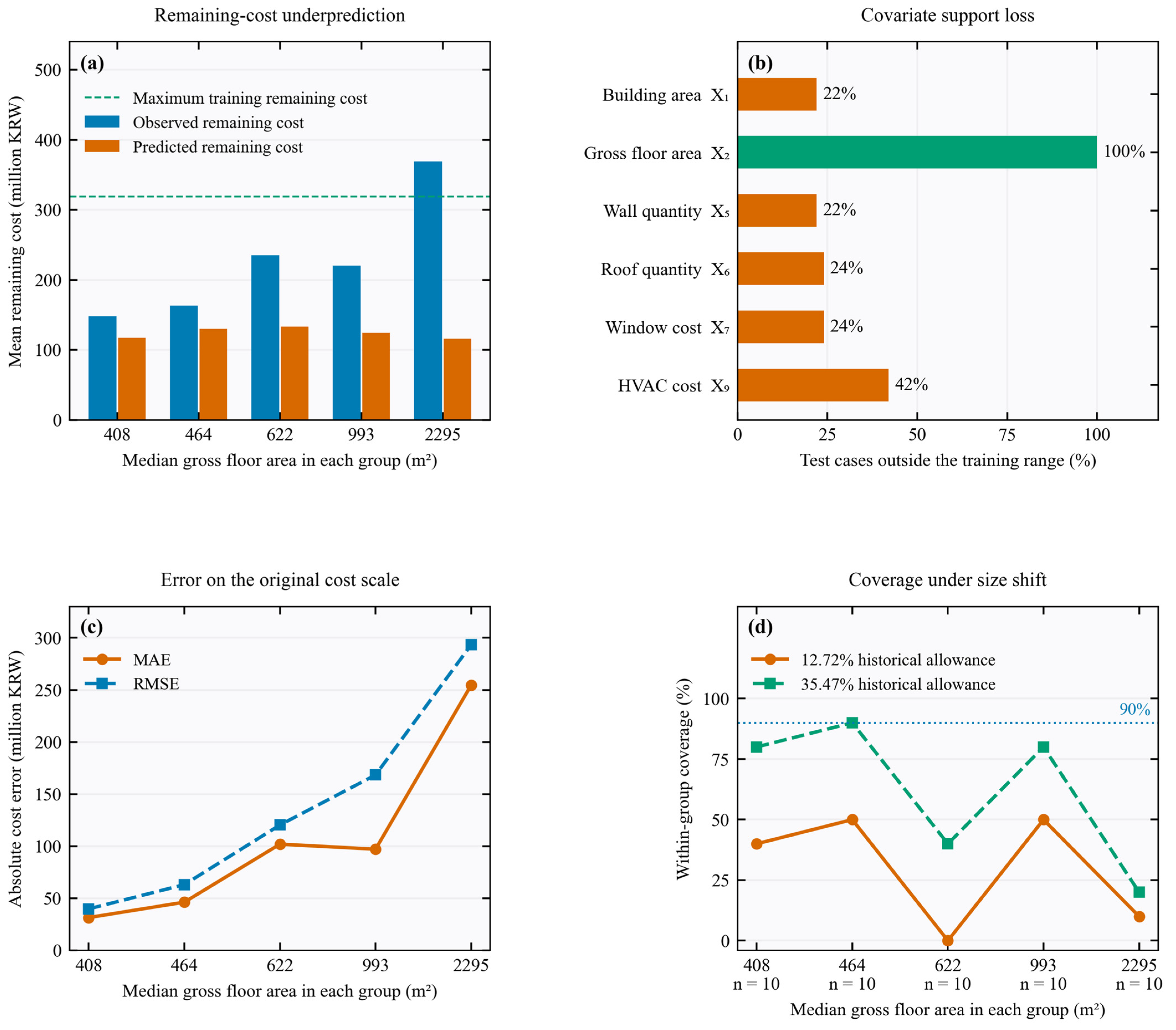
The largest-area holdout reveals a specific extrapolation problem (Figure 7; Table A11). All 50 test projects exceeded the training maximum X2 of 393.32 m2. Eleven had actual R above the training maximum of KRW 318.95 million, and 42% had X9 outside its training range. An unsmeared regression-tree ensemble averages training log-target values and cannot extrapolate R beyond the fitted target range; adding known C does not remove that limit. Reproduced holdout MAE was KRW 106.26 million, RMSE KRW 163.98 million, R-WAPE 46.74% and R squared −0.004. Even the historical 35.47% allowance covered only 31/50 cases (62%). In the ten largest test buildings, mean observed R was KRW 369.36 million versus the mean predicted R of KRW 116.18 million. These diagnostics support limited training support and target-range restriction as plausible contributors; they do not identify a causal effect of size or rule out omitted scope and price factors. This fixed-threshold stress check is not an independent calibration because the historical allowance used all 246 records; the disjoint experiment assesses calibration separately.
Panels (a), (c) and (d) show predictions, absolute errors and fixed-uplift coverage for five ordered area groups, each containing ten held-out projects and labeled by median area. Panel (b) shows out-of-range input frequencies. The fixed allowances in panel (d) were derived from the complete sample; the coverage results are not independent allowance calibration. Full results are shown in Table A11.
4.4. Empirical Contingency for Projects and Groups
For the flag-excluded reference class, single-project contingency was 13.87% at P80, 35.47% at P90 and 47.12% at P95 (Table 4, Panel A). The bootstrap interval for P90 was 23.70–42.89%. Treating the 12.72% fold-mean MAPE as an allowance covered only 79.7% of repeated case-mean predictions, rather than 90%. With grouping without replacement, P90 fell to 20.90% for five projects and 9.00% for 100, while the probability of aggregate underprediction rose from 52.44% to 99.97%. P90 gives reserve size; underprediction probability ignores magnitude. The complete n = 246 reference class required a 6.51% aggregate uplift relative to predicted cost. The MAPE calculated directly from the case-mean predictions was 12.51%.
P90 calculated separately within the five repetitions ranged from 34.19% to 37.01%; pooling all 1230 dependent held-out predictions gave 35.38%, compared with 35.47% from the 246 case-mean predictions (Table A12A). The observed comparison does not indicate a downward P90 effect from averaging predictions.
Figure 7.
Training support and remaining-cost errors for the largest-area holdout.
For the selected n = 246 route on its original partitions, training-only smearing reduced case-mean aggregate Y bias from −6.11% to −0.03% and retrospective P90 from 35.47% to 27.88% (Table 4B). However, fold-mean Y-MAPE increased from 12.72% to 15.16% and R-WAPE from 19.28% to 21.07%; Y-RMSE decreased from KRW 49.28 million to KRW 47.40 million. A smaller additional uplift therefore partly reflects a higher point prediction and is not evidence that every loss or budget outcome improves. The factors ranged from 1.062 to 1.189. These matched results directly assess the selected route, while the earlier n = 250 fixed-specification sensitivity remains in Table A10.
Table 4.
Contingency for project groups. (A). Tuned remaining-cost model. (B). Matched back-transformation sensitivity for the selected n = 246 route.
Figure 8a ranks project uplift as 100 × (Y/Ŷ − 1); negative values denote overprediction. Panel (b) gives empirical allowances with pointwise 95% bootstrap intervals, and (c) gives quantiles for sampled project groups. Table 4 reports aggregate underprediction probability. At 246 projects, only one aggregate ratio remains, so P80, P90 and P95 coincide. These retrospective estimates use the same records for calibration and description and provide no prospective coverage guarantee.
Figure 8.
Historical empirical budget contingency: (a) ranked project-level required cost uplifts; (b) contingency estimates by target non-overrun probability, with 95% bootstrap intervals; (c) P80, P90, and P95 contingency estimates by sampled project-group size.
With disjoint calibration and evaluation records, unsmeared empirical P90 allowances ranged from 16.39% to 43.63% and evaluation coverage ranged from 38/50 to 49/50 (76–98%; Figure 5b,c and Table A10). The descriptive mean coverage across ten overlapping splits was 89.8%; it is not a binomial estimate from 500 independent projects. Split 1 covered 47/50 (94%; exact 95% interval 83.45–98.75%), whereas split 3 covered 38/50 (76%; 61.83–86.94%). The finite-rank sensitivity achieved 82–98% coverage, with a descriptive mean of 91.4%. Table A10 also reports the matched smeared fits. The wide spread demonstrates calibration uncertainty within this archive and prevents the interpretation of the historical 35.47% as a fixed future P90 budget rule.
Conditional training-OOF calibration gave mean P90 allowances of 34.14% for log(R) + C, 34.34% for direct X1–X10 and 49.78% for direct X1–X6, with mean outer-test coverage of 89.36%, 89.93% and 89.36%, respectively (Table A13A). Separately seeded OOF folds gave mean P90 allowances of 33.98%, 33.56% and 51.01%, with mean coverage of 89.85%, 89.85% and 89.68%, respectively, for the same three routes. These estimates suggest how the assumed information boundary affects the required allowance, while retaining the selection and refit-size qualifications described in Section 3.6.
5. Discussion
5.1. Additional Cost Information and Model Performance
The added component costs improved both GA-weighted CBR and Extra Trees within this archive, while their difference in improvement remained uncertain. Previous CBR work emphasizes feature weighting, retention and robustness [9,11,12,14,15]; the smaller contrast after learned weighting is consistent with similarity design affecting the comparison. The additional ensemble comparisons reinforce the need to assess the whole selection procedure. Recent graph-based and TabPFN stacking studies [28,29] address different data structures and prediction targets, so their findings inform method choice rather than a direct accuracy ranking on the LH extract.
The nested benchmark evaluates selection within an explicit candidate pool and complements the original GA-CBR comparison of information changes. It retains weaker baselines and uncertainty around paired contrasts, which makes the consequences of selecting the lowest observed error visible. The candidate pool and screening decisions nevertheless reflect prior work with this archive; Section 5.5 states the resulting validation limits.
An observed cost component has two roles: it can be a predictor and it can be an amount added directly to a predicted remainder. Reporting Y and R together separates this accounting contribution from the learned prediction. A low total-cost percentage error can coexist with substantial error for the unknown amount, especially when R is small. This distinction gives the information comparison a practical interpretation even when the preferred estimator remains uncertain.
The timing of information determines how these comparisons can be used. Cost-estimate classifications relate accuracy to project definition [1,2,3]. For application to a new estimate, both the component costs and the insulation quantities would need a dated snapshot at the intended decision stage, with an independently defined outcome. The present experiments quantify performance conditional on the recorded inputs.
5.2. Errors in Total and Remaining Cost
The remaining-cost errors in Section 4.2 describe the modeling burden when C is known. Reporting those errors alongside common MAE and RMSE prevents the larger total-cost denominator from obscuring prediction uncertainty. The remaining-cost formulation can be chosen for its information boundary and accounting transparency; the paired comparison leaves its accuracy advantage over direct prediction uncertain.
Case 212 illustrates the denominator sensitivity of remaining-cost MAPE: subtracting known components left a small remainder, and removing the case would have improved MAPE much more than WAPE. Retaining it and reporting several error measures therefore gives a more complete view of model performance. Predicted-cost deciles and the comparisons of zero versus positive X5 values also showed heterogeneous error patterns. Field definitions and validation on new projects are needed before these patterns can justify cost adjustments or exclusion rules.
5.3. Using Model Errors to Examine Contingency
The historical MAPE allowance and P90 allowance answer different questions. The former averages absolute percentage errors; the latter summarizes the upper tail of observed-to-predicted cost ratios. Contingency studies and reference-class forecasting similarly distinguish risk allowance from average accuracy [7,8,43,44,45,46,47,48]. The separate calibration and evaluation experiment shows how uncertainty in an estimated quantile translates into variable coverage, even within the same archive.
The loss of coverage in the largest-area holdout calls for a review of comparable projects and model support before increasing a reserve. At portfolio scale, overestimates partly offset underestimates, reducing the required uplift, while negative aggregate bias made some shortfall more frequent. Reserve size and shortfall probability therefore describe different aspects of budget risk. Future common shocks would add dependence that historical grouping alone cannot assess.
An operational evaluation would define a justified comparison population, dated information sets and a common price basis, freeze the prediction procedure, and reserve separate records for allowance calibration and final evaluation. The present three-way experiment demonstrates the last step internally. The remaining data requirements are stated in Section 5.5.
5.4. Cost Uncertainty and Economic Feasibility
Energy-retrofit appraisal connects intervention costs to energy-performance outcomes and measures such as net present value (NPV), return on investment (ROI) and payback [51]. For a point estimate Ŷ and cost uplift q, the stressed initial investment is K(q) = Ŷ(1 + q). NPV equals the discounted sum of annual net savings over the chosen horizon less K(q). Discounted net ROI is NPV divided by K(q); with constant annual net savings S, simple payback is K(q)/S. The allowance is a risk-budget scenario, not expected expenditure. Earmarking an unspent reserve alone does not reduce realized NPV; the calculation assumes that the stressed capital amount is spent.
For illustration only, consider a KRW 100 million capital estimate, annual net savings of KRW 10 million, a 15-year horizon and a 5% discount rate. Discounted savings total KRW 103.80 million. At capital multipliers of 1.0000, 1.1272 and 1.3547, NPV is respectively +3.80, −8.92 and −31.67 million KRW; discounted net ROI is +3.80%, −7.92% and −23.38%; simple payback is 10.00, 11.27 and 13.55 years (Table 5). The 12.72% and 35.47% uplifts illustrate consequences of the historical quantities, not validated probabilities for this hypothetical project. A marginally feasible option can cross an acceptance threshold as cost assumptions change. A uniform multiplier need not reorder simple-payback rankings, whereas intervention-specific uncertainty or funding constraints can alter priorities. The LH archive contains no measured energy savings or intervention-specific cash flows, so actual ROI, NPV or ranking effects cannot be estimated. Those applications require joint uncertainty in costs, savings, tariffs, maintenance, service life and discount assumptions.
Table 5.
Illustrative capital-cost stress test for economic feasibility.
5.5. Limitations and Practical Use
The extract is not a probability sample, and the 419-record comparison shows differences in building scale, costs and recorded work content. We could not reconstruct the original extraction decisions, project implementation dates, cost-base dates or field-entry timestamps. Area conventions and recorded zeros remain incompletely documented. The exclusions and candidate development were retrospective. Joint family/target selection is nested within its stated candidate set, but earlier data-informed choices remain. The additional source-version analysis fixes one model setting; the training-OOF allowance analysis conditions on settings selected from the same outer-training data; and component perturbations are assumed error mechanisms. All are sensitivity analyses alongside the disjoint calibration experiment. Independent dated projects, measured energy savings and verified final-outturn records are still needed.
The supported use is to evaluate how a cost model is being interpreted. Information availability, remainder error, selection uncertainty and coverage under changed project composition should be reported together [52]. The largest-area holdout illustrates a concrete failure mode: models trained on smaller buildings substantially underpredicted the remainder. Dated and independently collected data, source-field verification and provider permission for wider access are necessary before extending the framework to actual budgeting or economic prioritization.
5.6. Information Collection and Decision-Time Uncertainty
The results suggest an information-collection sequence, as follows. First, verify the fields already used; distinguish true zero work from an unrecorded quantity, document the extent and specification of insulation and other retrofit work, and attach an estimate date and maturity status to each component amount. The X5 contrasts in Table A3 make scope verification relevant, while Table A11 shows why a new large project also needs comparable training cases. More detailed inputs alone cannot supply missing examples of large remaining costs. Until that support is established, an estimator should obtain a project-specific scope review and itemized estimate, rather than apply the historical 35.47% allowance automatically.
Second, collect information that can be known at the intended estimate date but is not included as a verified predictor here. Building use and occupancy can describe service requirements and constraints on working in an occupied building; region and site-access conditions can describe local procurement and execution conditions. Planned retrofit year, estimate date and component price-base dates can support a common price basis, while verified actual implementation dates are needed later to distinguish scheduling changes from price changes. Planned and actual dates must be stored separately. Detailed work packages, specifications, survey findings and procurement assumptions would help distinguish projects with similar floor areas but different remaining scope. These are candidate explanations for unexplained errors, not demonstrated causes of the observed block or size effects; this study has not estimated the accuracy gain from adding building use, region or retrofit year.
The available quantitative evidence for extra information concerns recorded component costs. On the matched Extra Trees comparison, adding X7–X10 reduced direct total-cost MAPE from 23.05% to 14.68%; predicting R and adding C gave 12.72%, without establishing an advantage over direct prediction. Under assumed prediction-time component error, remaining-route MAPE increased to 15.22% for mean-one lognormal σ = 0.30 and to 13.73% for independent uniform multipliers on [0.7, 1.3] (Table A13B). These sensitivities indicate that information quality matters, but they do not measure the benefit of collecting a particular new field. A future evaluation should add verified descriptor, scope and dated-cost groups incrementally on common partitions, retain only information available at the prediction date, and report changes in Y-MAPE, R-WAPE, bias and independently evaluated coverage. Dated cohorts and sufficiently represented building-use, regional and size groups would permit assessment of where a gain persists.
Finally, some realized information cannot be known with certainty when the estimate is prepared. Concealed deterioration may be discovered only during intrusive inspection or construction; later design changes, contractor outcomes and future price or schedule shocks may remain uncertain. Surveys and documented assumptions can reduce parts of this uncertainty, but realized changes and final expenditure must remain outcomes for later evaluation. At the decision date, their plausible consequences should be represented by explicit scenarios and a separately calibrated allowance, with the estimate updated when new evidence becomes available. This separates missing but collectable descriptors from uncertainty that remains at the chosen decision stage, and prevents future information from being used as if it were already observed.
6. Conclusions
The data support three bounded findings. First, adding four recorded component costs reduced error for both GA-weighted CBR and Extra Trees, while the primary corrected interval did not establish a difference in the magnitude of improvement. Second, the original remaining-cost route had 19.28% R-WAPE and 29.42% R-MAPE despite a reconstructed total-cost MAPE of 12.72%; its paired advantage over direct prediction was uncertain. Third, the model transferred poorly to the largest-area holdout, where R-WAPE reached 46.74% and a 35.47% historical allowance covered only 62% of cases. The extract also differed from the other records in the research archive.
The methodological implication is an evaluation sequence that distinguishes the information observed, the amount predicted and the allowance evaluated. Joint inner selection makes the candidate comparison explicit, while separate calibration and evaluation expose uncertainty in coverage. This sequence connects model assessment to the decisions needed before a contingency rate can be applied.
Smearing reduced the additional historical uplift while worsening relative prediction errors, showing that the point forecast and reserve must be assessed together. The illustrative economic calculation similarly shows how spending a cost allowance can turn a marginally positive NPV negative. Applying that calculation to actual retrofit choices requires independently assessed savings and cost outcomes.
Prospective use requires validation on independently collected, dated projects with documented cost versions, price bases and selection rules.
Future studies should freeze the model and information boundary before assessing separate calibration and evaluation cohorts, including larger buildings. Economic applications also need independently validated energy savings, tariffs, maintenance and service-life assumptions.
Author Contributions
Conceptualization, N.K.; methodology, N.K.; software, N.K.; formal analysis, N.K.; validation, N.K., H.M. and S.P.; investigation, J.K. and S.P.; data curation, J.K.; resources, J.K.; visualization, N.K. and J.K.; writing—original draft preparation, N.K.; writing—review and editing, N.K., J.K., H.M., Y.A. and S.P.; supervision, H.M. and Y.A.; project administration, Y.A. and S.P.; funding acquisition, N.K. All authors have read and agreed to the published version of the manuscript.
Funding
This work was supported by the National Research Foundation of Korea (NRF) grant funded by the Korean Government (MSIT) (RS-2024-00344868).
Institutional Review Board Statement
Not applicable. This study analyzed deidentified project cost records and involved no human participants, personal data, or intervention.
Informed Consent Statement
Not applicable.
Data Availability Statement
The project records were provided by the Korea Land and Housing Corporation. The authors have not established permission to redistribute the record-level extract or its linked source workbook in a public repository. Access requests may be directed to the corresponding author and remain subject to the provider’s authorization. Analysis code, data definitions, aggregate results and the analysis specification can be supplied on reasonable request. Appendix A contains the principal aggregate audit and validation results. The reproduction of record-level predictions requires authorized access; no public dataset deposit is claimed.
Conflicts of Interest
The authors declare no conflicts of interest.
Appendix A. Supporting Methods and Results
The appendix reports data definitions, retrospective screening, model-selection details, sampling comparisons and supporting validation results. Table A1, Table A2, Table A3, Table A4, Table A5, Table A6 and Table A7 report data definitions, screening and the primary analyses; Table A8, Table A9, Table A10 and Table A11 report the archive comparison, expanded benchmark, calibration and large-area diagnostics; Table A12 and Table A13 report aggregation, source-version, calibration and input-perturbation checks. Monetary units and aggregation levels are stated for each panel.
Unless a panel labels KRW, monetary displays use USD converted from nominal KRW at USD 1 = KRW 1383.60 (basic exchange rate, 24 August 2026). The conversion is a reporting scale only; percentage metrics are unchanged, while labeled log1p sensitivities remain scale-dependent.
Data provenance and notation. The analysis uses a 250-record LH public-building retrofit extract. X1 is recorded building area and X2 is recorded gross floor area. X3 equals 2022 minus completion year; 2022 is an age reference, not the retrofit or collection year.
Appendix A.1. Data Definitions and Supporting Tables
Table A1.
Data definitions (Panel (A)). Descriptive statistics (Panel (B)). Primary descriptive statistics (Panel (C)). Recorded field provenance and decision-time availability (Panel (D)).
Table A2.
Comparator models (Panel (A)). Selected model settings (Panel (B)).
Table A3.
Errors by insulation quantity (Panel (A)). Nearest neighbor support (Panel (B)). Case level calibration (Panel (C)). Nearest-neighbor geometry (Panel (D)).
Table A4.
Feature importance (Panel (A)). Selection loss sensitivity (Panel (B)).
Table A5.
Project composition.
Table A6.
Data quality sensitivity (Panel (A)). Area and floor checks (Panel (B)). Component share groups (Panel (C)). Predicted cost deciles (Panel (D)). Preprocessing sensitivity (Panel (E)). Remaining cost sensitivity (Panel (F)). Retrospective screening audit (Panel (G)).
Table A7.
Composition holdouts (Panel (A)). Example predictions (Panel (B)).
Table A8.
Included versus other records in the research archive (Panel (A)). Recorded scope and floor composition (Panel (B)).
As a supplementary archive check, the 15 test-case profiles published in Table 6 of [27] were compared using building area, gross floor area, completion year and floor count. Areas were compared within the rounding tolerance of the published two-decimal values, with exact year and floor-count agreement. None matched the 250-record extract; 14 had unique four-field matches among the other 169 archive records. These are profile matches, not confirmation of identical cost entries. This limited check supports a connection with the retained archive but does not establish the full record-level overlap with the published 401-case sample or reconstruct the historical selection procedure.
Table A9.
Additional common-partition family and target benchmark (Panel (A)). Search settings and preprocessing (Panel (B)).
Table A10.
Disjoint calibration and evaluation (Panel (A)). Back-transformation and allowance summaries (Panel (B)). Archived fixed-model sensitivity (Panel (C)).
Table A11.
Error within the largest-area holdout.
The expanded benchmark uses 25 common outer partitions, and the three-way design uses ten separately seeded random partitions of the available IDs (seeds and full grids are available on request; see the Data Availability Statement). Within each three-way split the ID sets are disjoint, while repetitions reuse records. Recalculated metrics and split membership were checked against saved predictions. Nominal KRW MAE/RMSE are computed within each outer test fold before averaging. Code and aggregate outputs can be supplied on request; source records and individual predictions remain access-controlled.
Appendix A.2. Reproducibility Details
Project-quantile intervals use 10,000 case-bootstrap draws with seed 20291807. Subset contingency uses 10,000 draws per intermediate size, without replacement within each draw, with seed 20292807. Composition-test P90 intervals use 10,000 draws and seed 20293807 plus the test index, numbered 1–6. Historical quantiles use NumPy linear interpolation; the new rank-46 sensitivity explicitly uses an order statistic instead. Analysis code and archived aggregate results are available from the corresponding author on reasonable request; regenerating project-level diagnostics requires authorized access to the source data.
The fixed smearing sensitivity uses all 250 cases, X1–X10 and log(R). Fivefold inner out-of-fold residuals (shuffle seed 1) estimate the mean exponentiated log residual. Extra Trees uses 250 trees, default hyperparameters and seed 0; outer repeated fivefold validation uses seed 42. These results use a different protocol from the tuned primary model.
The primary case-mean Y-MAPE is 12.51285%, distinct from fold-mean Y-MAPE 12.72%. Case-mean aggregate bias is −6.10922% for Y and −8.78465% for R. Predicted cost and project uplift have Spearman correlation 0.15902; this weak positive association does not establish a unique cause of the nonmonotonic P80. The full-sample X5 MAPE ratios 2.24 and 1.30 compare repeated-validation case-means with the separate ordered holdout; the support-group difference interval is a distinct analysis.
Appendix A.3. Supporting Figures
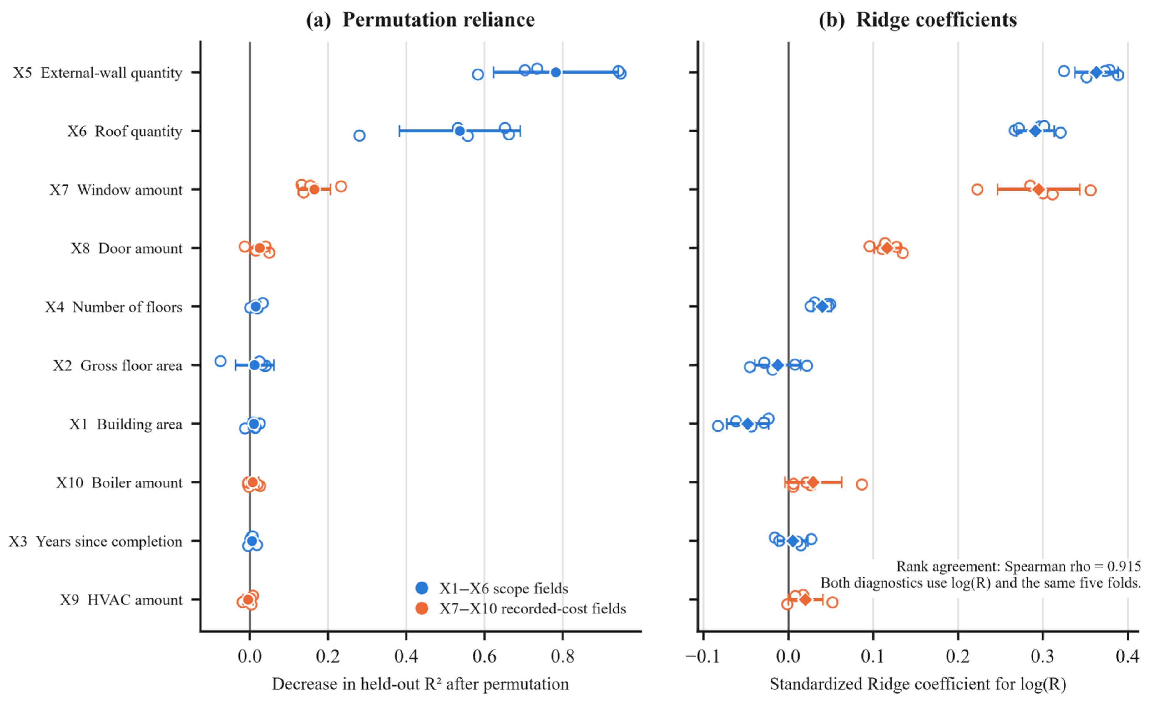
Figure A1 reports rank correlations and marginal cost distributions in the unfiltered sample. Figure A2 compares permutation-based Extra Trees reliance with standardized Ridge coefficients; these are association diagnostics, not causal effects.
Figure A1.
Data correlations and distributions.
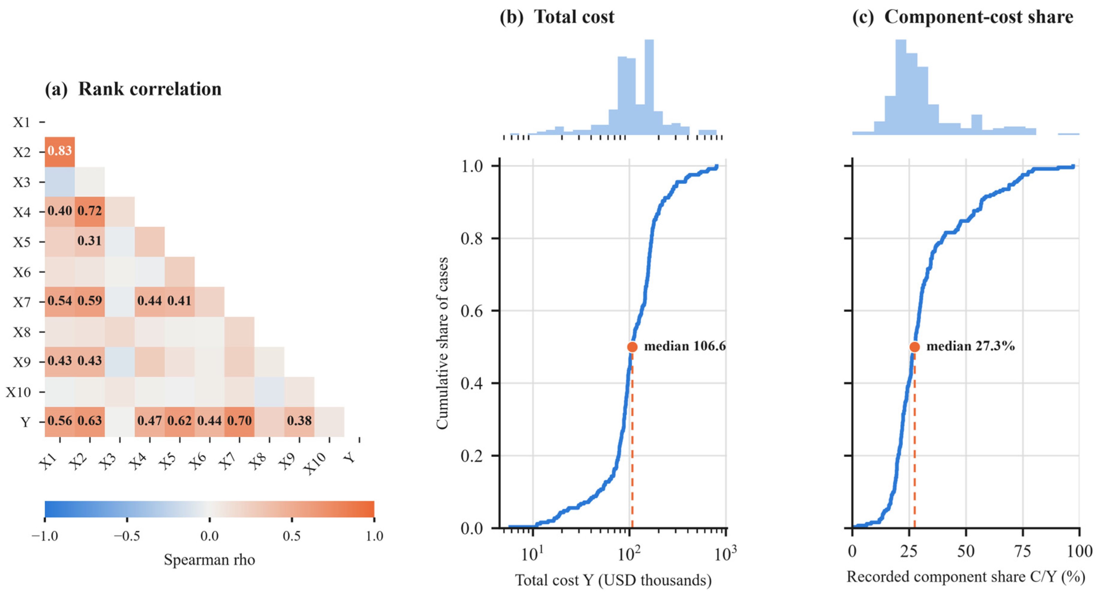
Figure A2.
Feature importance comparisons.
Appendix A.4. Additional Sensitivity Analyses
Table A12.
Aggregation and source-version sensitivity. (A). Historical P90 under alternative aggregation. Aggregation and source-version sensitivity. (B). Fixed-model source-version substitution.
Table A13.
Conditional calibration and component-cost perturbation. (A). Training-OOF allowance check. Conditional calibration and component-cost perturbation. (B). Prediction-time input sensitivity.
References
- AACE International. Cost Estimate Classification System; Recommended Practice No. 17R-97; AACE International: Morgantown, WV, USA, 2020; Available online: https://web.aacei.org/docs/default-source/toc/toc_17r-97.pdf (accessed on 25 August 2026).
- AACE International. Cost Estimate Classification System—As Applied in Engineering, Procurement, and Construction for the Building and General Construction Industries; Recommended Practice No. 56R-08; AACE International: Morgantown, WV, USA, 2020; Available online: https://web.aacei.org/docs/default-source/toc/toc_56r-08.pdf (accessed on 25 August 2026).
- Cho, C.-S.; Gibson, G.E., Jr. Building project scope definition using project definition rating index. J. Archit. Eng. 2001, 7, 115–125. [Google Scholar] [CrossRef] [Scilit]
- Aamodt, A.; Plaza, E. Case-based reasoning: Foundational issues, methodological variations, and system approaches. AI Commun. 1994, 7, 39–59. [Google Scholar] [CrossRef] [Scilit]
- Kaufman, S.; Rosset, S.; Perlich, C.; Stitelman, O. Leakage in data mining: Formulation, detection, and avoidance. ACM Trans. Knowl. Discov. Data 2012, 6, 15. [Google Scholar] [CrossRef] [Scilit]
- Kapoor, S.; Narayanan, A. Leakage and the reproducibility crisis in machine-learning-based science. Patterns 2023, 4, 100804. [Google Scholar] [CrossRef] [Scilit] [PubMed]
- Bakhshi, P.; Touran, A. An overview of budget contingency calculation methods in construction industry. Procedia Eng. 2014, 85, 52–60. [Google Scholar] [CrossRef] [Scilit]
- Ko, T.; Le, C.; Jeong, H.D.; Choi, K. Enhancing reliability of construction contingency estimation at the scoping phase through historical cost data analysis. ASCE-ASME J. Risk Uncertain. Eng. Syst. Part A Civ. Eng. 2024, 10, 04024068. [Google Scholar] [CrossRef] [Scilit]
- Kim, K.J.; Kim, K. Preliminary cost estimation model using case-based reasoning and genetic algorithms. J. Comput. Civ. Eng. 2010, 24, 499–505. [Google Scholar] [CrossRef] [Scilit]
- Ahn, J.; Park, M.; Lee, H.-S.; Ahn, S.J.; Ji, S.-H.; Song, K.; Son, B.-S. Covariance effect analysis of similarity measurement methods for early construction cost estimation using case-based reasoning. Autom. Constr. 2017, 81, 254–266. [Google Scholar] [CrossRef] [Scilit]
- Ji, S.-H.; Ahn, J.; Lee, E.-B.; Kim, Y. Learning method for knowledge retention in CBR cost models. Autom. Constr. 2018, 96, 65–74. [Google Scholar] [CrossRef] [Scilit]
- Jung, S.; Pyeon, J.-H.; Lee, H.-S.; Park, M.; Yoon, I.; Rho, J. Construction cost estimation using a case-based reasoning hybrid genetic algorithm based on local search method. Sustainability 2020, 12, 7920. [Google Scholar] [CrossRef] [Scilit]
- Kwon, N.; Song, K.; Ahn, Y.; Park, M.; Jang, Y. Maintenance cost prediction for aging residential buildings based on case-based reasoning and genetic algorithm. J. Build. Eng. 2020, 28, 101006. [Google Scholar] [CrossRef] [Scilit]
- Uysal, F.; Sonmez, R. Bootstrap aggregated case-based reasoning method for conceptual cost estimation. Buildings 2023, 13, 651. [Google Scholar] [CrossRef] [Scilit]
- Xiao, X.; Skitmore, M.; Yao, W.; Ali, Y. Improving robustness of case-based reasoning for early-stage construction cost estimation. Autom. Constr. 2023, 151, 104777. [Google Scholar] [CrossRef] [Scilit]
- Shen, C.; Meng, P.; Shen, J.; Sun, G. A construction cost estimation system based on case-based reasoning and exponential smoothing. J. Build. Eng. 2025, 113, 114120. [Google Scholar] [CrossRef] [Scilit]
- Fung, J.F.; Sattar, S.; Butry, D.T.; McCabe, S.L. Machine learning methods for predicting seismic retrofit costs. Presented at the 17th World Conference on Earthquake Engineering, Sendai, Japan, 27 September–2 October 2021; Available online: https://tsapps.nist.gov/publication/get_pdf.cfm?pub_id=929595 (accessed on 25 August 2026).
- Alshboul, O.; Shehadeh, A.; Almasabha, G.; Almuflih, A.S. Extreme gradient boosting-based machine learning approach for green building cost prediction. Sustainability 2022, 14, 6651. [Google Scholar] [CrossRef] [Scilit]
- Elmousalami, H.H. Artificial intelligence and parametric construction cost estimate modeling: State-of-the-art review. J. Constr. Eng. Manag. 2020, 146, 03119008. [Google Scholar] [CrossRef] [Scilit]
- He, X.; Liu, R.; Anumba, C.J. Data-driven insights on the knowledge gaps of conceptual cost estimation modeling. J. Constr. Eng. Manag. 2021, 147, 04020165. [Google Scholar] [CrossRef] [Scilit]
- Gill, E.Z.; Cardone, D.; Amelio, A. Revolutionizing the construction industry by cutting edge artificial intelligence approaches: A review. Front. Artif. Intell. 2024, 7, 1474932. [Google Scholar] [CrossRef] [Scilit] [PubMed]
- Karadimos, P.; Anthopoulos, L. A taxonomy of machine learning techniques for construction cost estimation. Innov. Infrastruct. Solut. 2024, 9, 420. [Google Scholar] [CrossRef] [Scilit]
- Zhang, W. Applications of machine learning and artificial intelligence in construction project cost prediction: A scientometric analysis and qualitative review. Front. Built Environ. 2026, 12, 1867673. [Google Scholar] [CrossRef] [Scilit]
- Lee, J.G.; Lee, H.S.; Park, M.; Seo, J.O. Early-stage cost estimation model for power generation project with limited historical data. Eng. Constr. Archit. Manag. 2022, 29, 2599–2614. [Google Scholar] [CrossRef] [Scilit]
- Sharma, V.; Zaki, M.; Jha, K.N.; Krishnan, N.M.A. Machine learning-aided cost prediction and optimization in construction operations. Eng. Constr. Archit. Manag. 2022, 29, 1241–1257. [Google Scholar] [CrossRef] [Scilit]
- Wang, R.; Salleh, H.; Lyu, J.; Abdul-Samad, Z.; Radzuan, N.F.M.; Wen, K.C. Application and prospect of machine learning techniques in cost estimation of building projects. Eng. Constr. Archit. Manag. 2025, 32, 8445–8471. [Google Scholar] [CrossRef] [Scilit]
- Park, S.; Park, S.; Jang, H.; Ahn, Y.; Kwon, N. Computing green remodeling construction cost for public buildings based on genetic algorithm and case-based reasoning. Dev. Built Environ. 2025, 22, 100655. [Google Scholar] [CrossRef] [Scilit]
- Wang, J.; Gu, Q.; Chileshe, N. Construction cost prediction using a fused loss–enhanced hybrid GCN–GAT–MLP approach. Eng. Constr. Archit. Manag. 2025, 1–24, advance online publication. [Google Scholar] [CrossRef] [Scilit]
- Wang, J.; Gu, Q.; Chileshe, N. Construction cost prediction using TabPFN-based stacking model with SHAP analysis. Eng. Constr. Archit. Manag. 2026, 1–25, advance online publication. [Google Scholar] [CrossRef] [Scilit]
- Kim, G.-H.; An, S.-H.; Kang, K.-I. Comparison of construction cost estimating models based on regression analysis, neural networks, and case-based reasoning. Build. Environ. 2004, 39, 1235–1242. [Google Scholar] [CrossRef] [Scilit]
- Duan, N. Smearing estimate: A nonparametric retransformation method. J. Am. Stat. Assoc. 1983, 78, 605–610. [Google Scholar] [CrossRef]
- Manning, W.G. The logged dependent variable, heteroscedasticity, and the retransformation problem. J. Health Econ. 1998, 17, 283–295. [Google Scholar] [CrossRef] [Scilit] [PubMed]
- Varma, S.; Simon, R. Bias in error estimation when using cross-validation for model selection. BMC Bioinform. 2006, 7, 91. [Google Scholar] [CrossRef] [Scilit] [PubMed]
- Cawley, G.C.; Talbot, N.L.C. On over-fitting in model selection and subsequent selection bias in performance evaluation. J. Mach. Learn. Res. 2010, 11, 2079–2107. [Google Scholar]
- Nadeau, C.; Bengio, Y. Inference for the generalization error. Mach. Learn. 2003, 52, 239–281. [Google Scholar] [CrossRef] [Scilit]
- Varoquaux, G. Cross-validation failure: Small sample sizes lead to large error bars. NeuroImage 2018, 180, 68–77. [Google Scholar] [CrossRef] [Scilit] [PubMed]
- Larocque, R.; Boulé, A.-M.; Cappart, Q. Estimating road construction costs with explainable machine learning. Inf. J. Appl. Anal. 2025, 55, 137–153. [Google Scholar] [CrossRef] [Scilit]
- Moreno-Torres, J.G.; Raeder, T.; Alaiz-Rodriguez, R.; Chawla, N.V.; Herrera, F. A unifying view on dataset shift in classification. Pattern Recognit. 2012, 45, 521–530. [Google Scholar] [CrossRef] [Scilit]
- Sahigara, F.; Mansouri, K.; Ballabio, D.; Mauri, A.; Consonni, V.; Todeschini, R. Comparison of different approaches to define the applicability domain of QSAR models. Molecules 2012, 17, 4791–4810. [Google Scholar] [CrossRef] [Scilit] [PubMed]
- Tibshirani, R.J.; Foygel Barber, R.; Candes, E.; Ramdas, A. Conformal prediction under covariate shift. Adv. Neural Inf. Process. Syst. 2019, 32, 2526–2536. [Google Scholar]
- Barber, R.F.; Candes, E.J.; Ramdas, A.; Tibshirani, R.J. Predictive inference with the jackknife+. Ann. Stat. 2021, 49, 486–507. [Google Scholar] [CrossRef] [Scilit]
- Angelopoulos, A.N.; Bates, S. Conformal prediction: A gentle introduction. Found. Trends Mach. Learn. 2023, 16, 494–591. [Google Scholar] [CrossRef] [Scilit]
- Touran, A. Calculation of contingency in construction projects. IEEE Trans. Eng. Manag. 2003, 50, 135–140. [Google Scholar] [CrossRef] [Scilit]
- Bae, J. Supervised learning to covering cost risk through post-construction evaluation of transportation projects by project delivery methods. Eng. Constr. Archit. Manag. 2025, 32, 5863–5884. [Google Scholar] [CrossRef] [Scilit]
- Nindartin, A.; Park, S.-J.; Lee, K.-T.; Kim, J.-H.; Rostiyanti, S.F. Prediction of cost contingency in construction projects by introducing machine learning algorithms. J. Civ. Eng. Manag. 2025, 31, 860–880. [Google Scholar] [CrossRef] [Scilit]
- Sihombing, L.B.; Saputra, B. Optimizing contingency cost for mid-scale contractors: An integrated Delphi and Monte Carlo method. Eng. Constr. Archit. Manag. 2026, 33, 7904–7919. [Google Scholar] [CrossRef] [Scilit]
- Flyvbjerg, B.; Holm, M.S.; Buhl, S. Underestimating costs in public works projects: Error or lie? J. Am. Plan. Assoc. 2002, 68, 279–295. [Google Scholar] [CrossRef] [Scilit]
- Flyvbjerg, B. From Nobel Prize to project management: Getting risks right. Proj. Manag. J. 2006, 37, 5–15. [Google Scholar] [CrossRef] [Scilit]
- Seoul Money Brokerage Services. Basic Exchange Rate: August 24, 2026. Available online: http://www.smbs.co.kr/Eng/ExRate/StdExRate.jsp (accessed on 24 August 2026).
- Hooker, G.; Mentch, L.; Zhou, S. Unrestricted permutation forces extrapolation: Variable importance requires at least one more model, or there is no free variable importance. Stat. Comput. 2021, 31, 82. [Google Scholar] [CrossRef] [Scilit]
- Piras, G.; Muzi, F.; Ziran, Z. A data-driven model for the energy and economic assessment of building renovations. Appl. Sci. 2025, 15, 8117. [Google Scholar] [CrossRef] [Scilit]
- Collins, G.S.; Moons, K.G.M.; Dhiman, P.; Riley, R.D.; Beam, A.L.; Van Calster, B.; Ghassemi, M.; Liu, X.; Reitsma, J.B.; Van Smeden, M.; et al. TRIPOD+AI statement: Updated guidance for reporting clinical prediction models that use regression or machine learning methods. BMJ 2024, 385, e078378. [Google Scholar] [CrossRef] [Scilit] [PubMed]
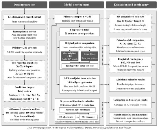
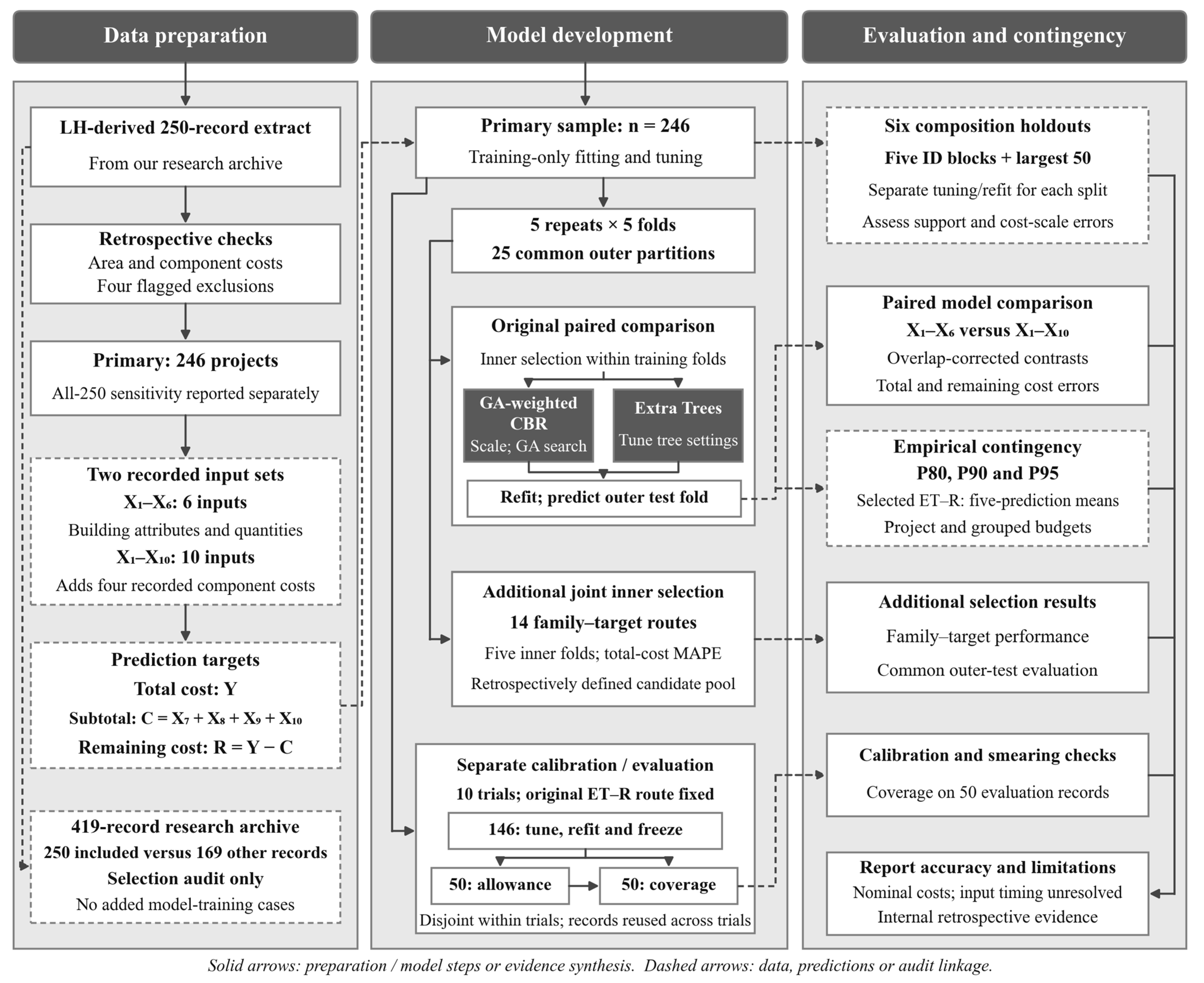
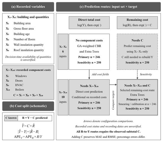
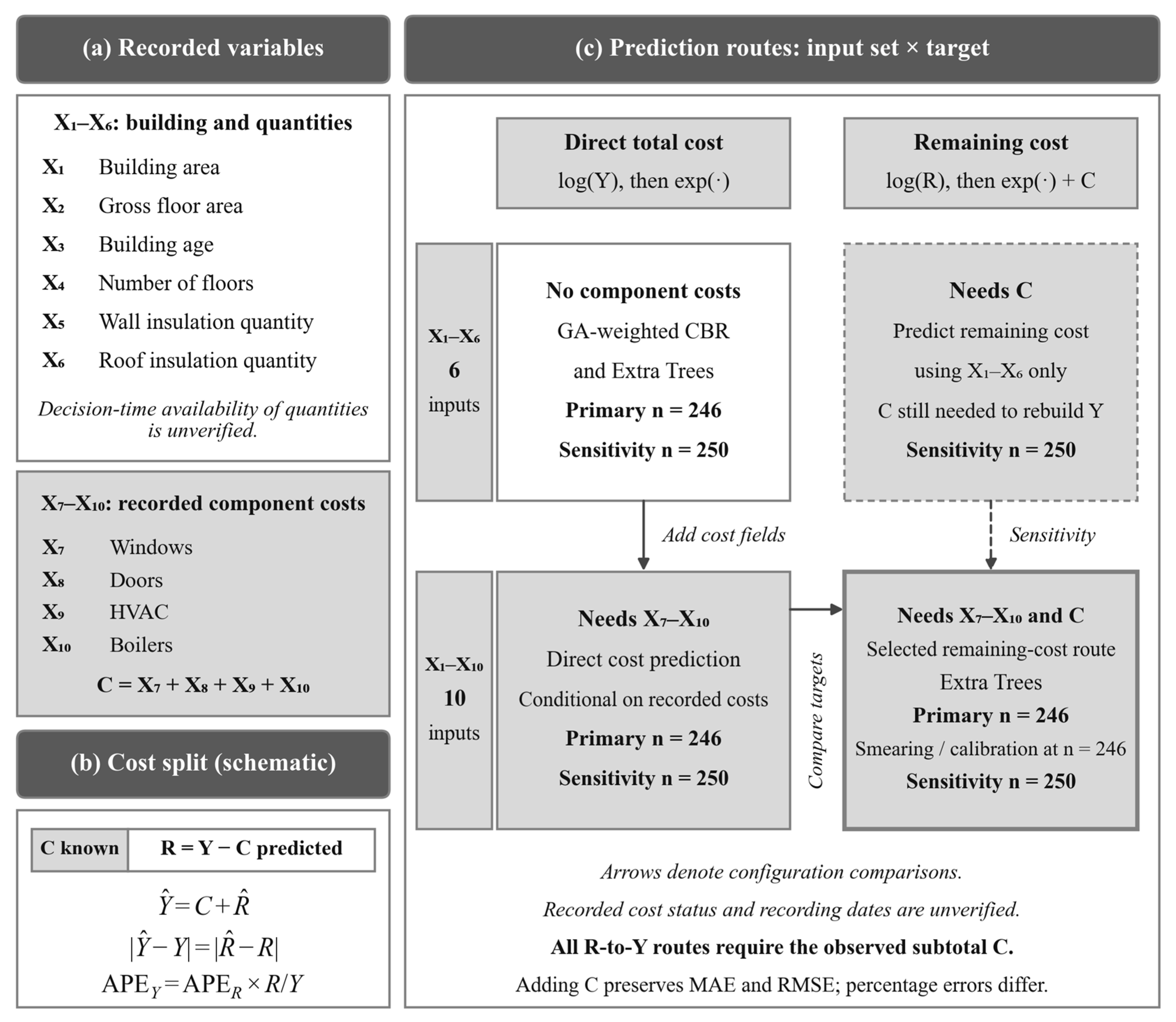
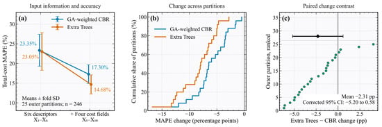
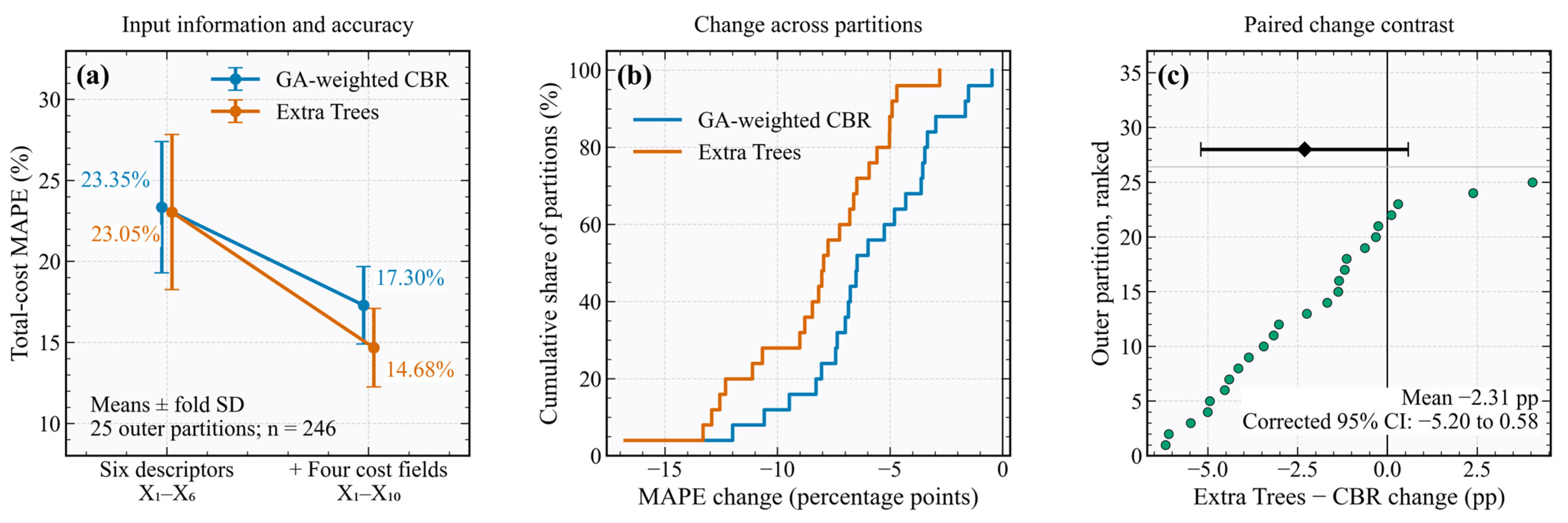
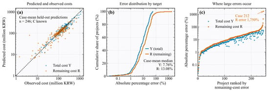
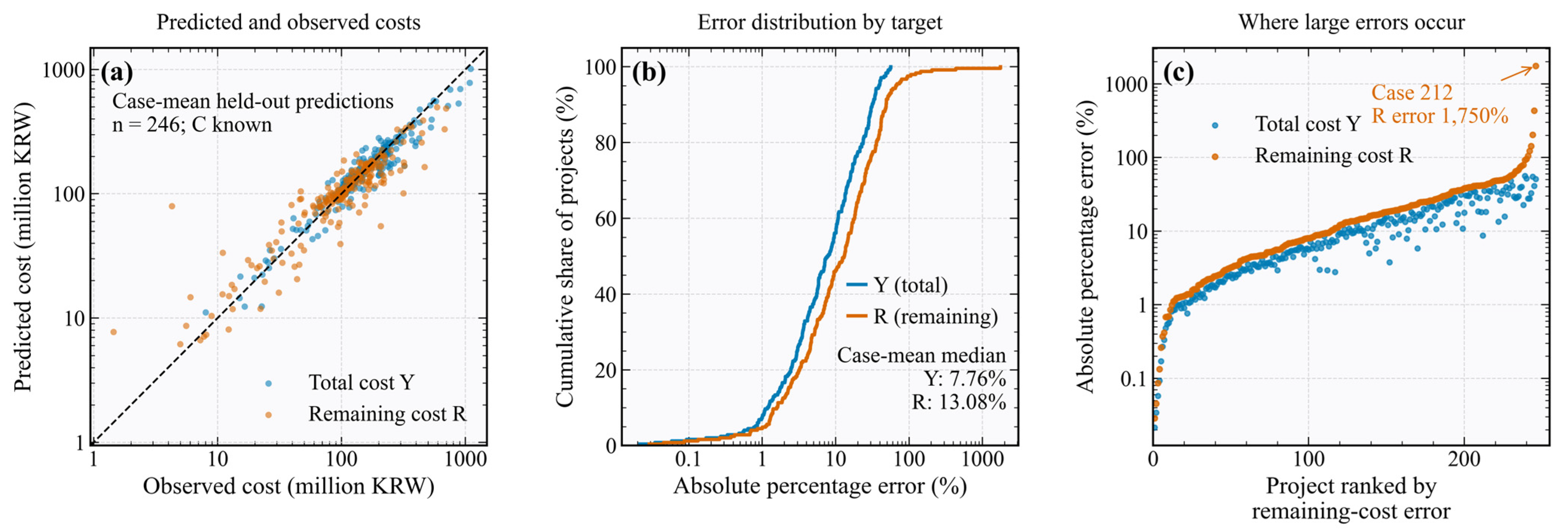
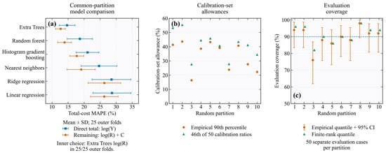
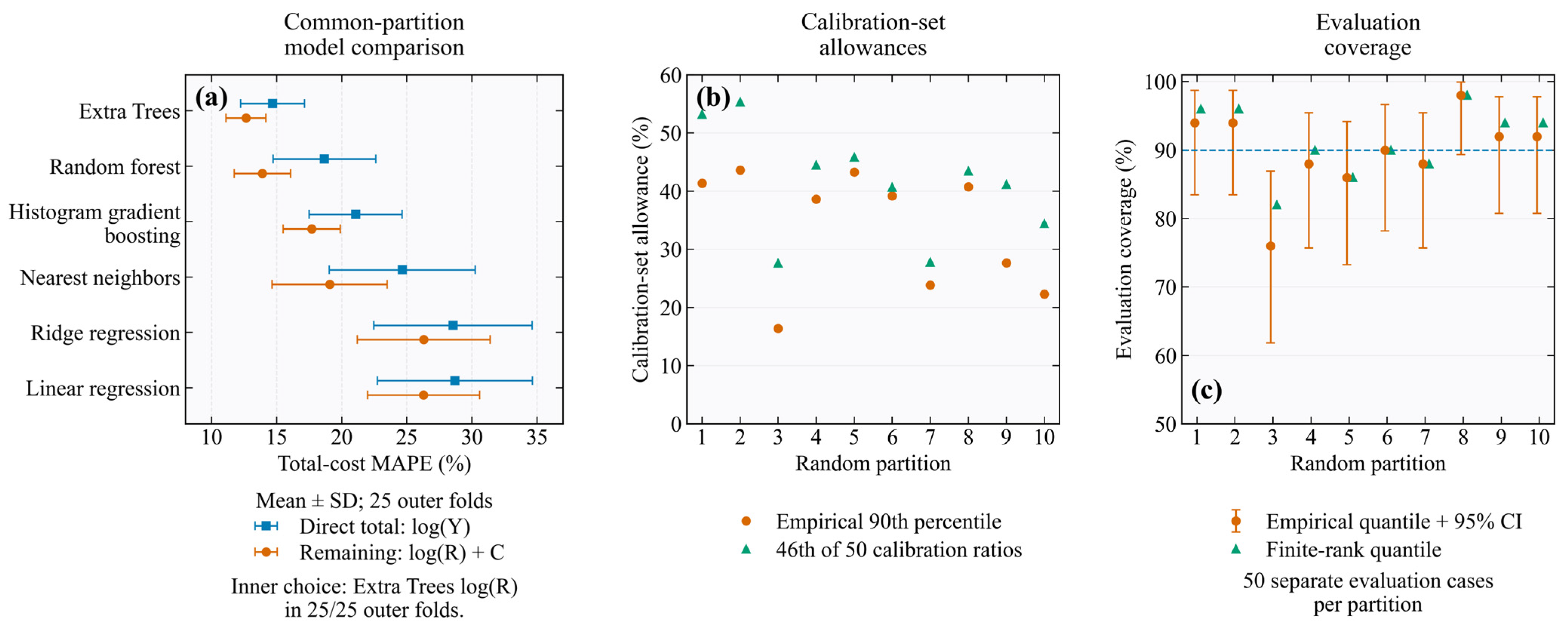
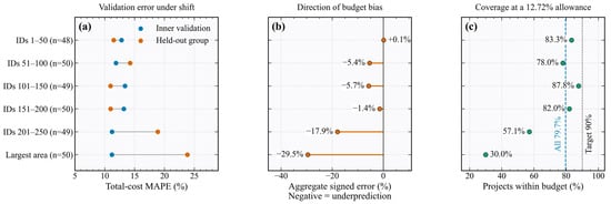
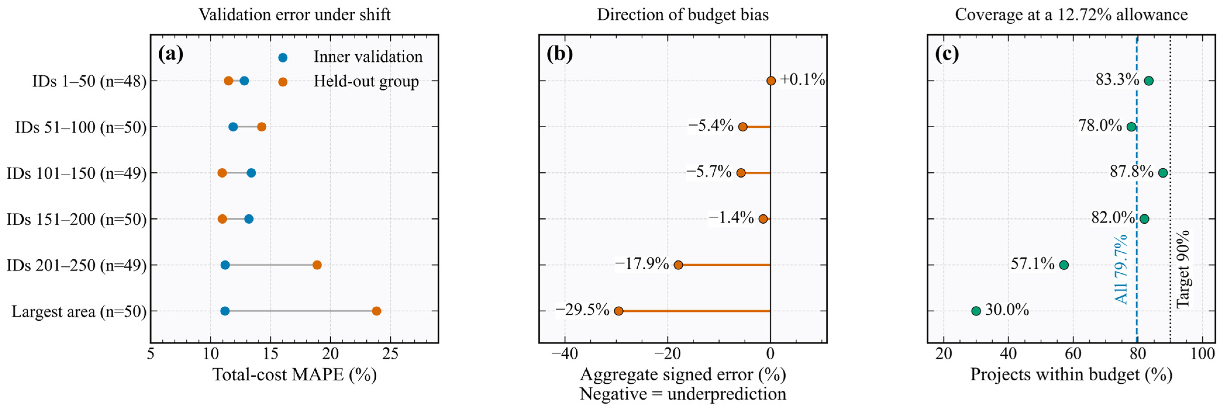
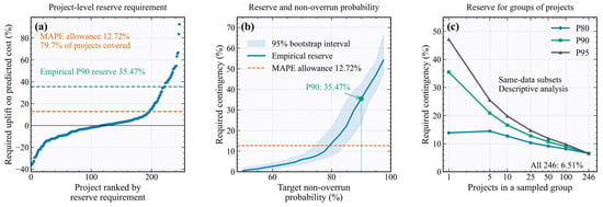
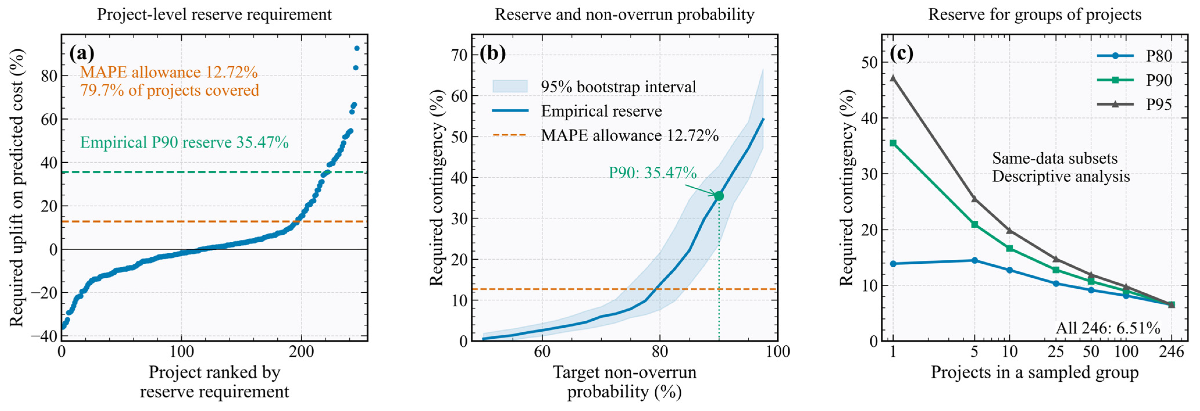

Disclaimer/Publisher’s Note: The statements, opinions and data contained in all publications are solely those of the individual author(s) and contributor(s) and not of MDPI and/or the editor(s). MDPI and/or the editor(s) disclaim responsibility for any injury to people or property resulting from any ideas, methods, instructions or products referred to in the content. |
© 2026 by the authors. Licensee MDPI, Basel, Switzerland. This article is an open access article distributed under the terms and conditions of the Creative Commons Attribution (CC BY) license.