Grouping-Driven Production Scheduling Optimization for Precast Concrete Components

Abstract

Precast component production is an important part of industrialization in construction. However, in actual production, it often faces problems such as high resource occupation, long production cycles, and high delivery costs caused by unreasonable scheduling arrangements. This study proposes a hybrid multi-objective optimization framework that combines Q-learning with the non-dominated sorting genetic algorithm, termed QL-NSGA-II, to address the highly coupled problem of component grouping on pallets and production scheduling in precast component manufacturing. The model aims to collaboratively minimize the number of pallets used, the makespan, and the penalty cost. The algorithm constructs a dual Q-table Markov decision architecture, in which the agent adaptively coordinates PC component grouping and scheduling strategies based on reward feedback from the evolutionary state. Through extreme-value tests on multiple benchmark instances from the literature, the results show that the proposed QL-NSGA-II not only achieves the accuracy of the benchmark solutions, but also, in some cases, reduces the makespan and penalty cost by 34.77% and 60.24%, respectively, compared with existing benchmark algorithms. In a real industrial order experiment with 87 components, the algorithm notably outperforms the comparison algorithms across comprehensive convergence metrics such as hypervolume and inverted generational distance, confirming its favorable practical application potential for balancing pallet resource consumption and flow cycle.

1. Introduction

With the rapid advancement of building industrialization, prefabricated buildings have been widely adopted worldwide owing to their advantages including shortened construction schedules, reduced environmental pollution and controllable quality [1]. As a core component of the prefabricated construction supply chain, the factory production of precast concrete (PC) elements directly determines the overall delivery efficiency and manufacturing cost of projects [2,3]. Nevertheless, most manufacturers of precast concrete elements are still confronted with common bottlenecks such as relatively low production efficiency, insufficient resource utilization and high energy consumption, which hinder the further development of the industry [4].

From the perspective of production processes, the manufacturing of PC elements is essentially a typical two-stage coupled optimization problem. Most PC elements are two-dimensional rectangular parts. Before entering the production line, different elements from multiple orders need to be arranged on pallets of fixed dimensions. This falls within the scope of the two-dimensional rectangular packing problem, whose primary objective is to maximize pallet area utilization and reduce the quantity of pallets used [5]. The second stage is production scheduling. The pallets carrying the components must sequentially pass through multiple processes such as reinforcement placement, concrete casting, curing, and demolding, and PC repairing. Since different processes may be equipped with different numbers of parallel machines (or workstations), this stage constitutes a typical hybrid flow shop scheduling problem [6]. The two stages are not independent of each other. The spatial layout of elements on pallets can directly affect the processing duration of subsequent procedures, creating a strong coupling relationship between space and time.

In existing research and engineering practice, grouping and production scheduling are generally treated as two separate problems and solved sequentially. Such a decomposed local optimization approach tends to trigger the barrel effect on production lines, resulting in workstation idleness and disrupted material flow rhythms [7]. Although numerous studies have conducted in-depth investigations into two-dimensional grouping or flow shop scheduling separately, research that integrates spatial grouping and temporal scheduling for the PC element scenario remains insufficient. Few studies have simultaneously achieved multi-dimensional balance among production efficiency, resource input and delivery cost, which makes it difficult to support the globally optimal operation of PC element production lines. Therefore, research on the joint optimization of two-dimensional grouping and hybrid flow shop scheduling carries important theoretical value and engineering significance for shortening the production cycle of PC elements, improving production line throughput and achieving energy conservation and emission reduction in the curing stage [5].

To address the above research gaps, this paper investigates the joint optimization of grouping and scheduling for PC components. The main contributions are outlined as follows:

1. A joint optimization mathematical model for PC component grouping and scheduling (PC-GS) is established. By mapping the spatial layout of PC components on the pallet into the processing parameters of subsequent processes, this model formulates a coupling mechanism between spatial grouping and temporal scheduling.

2. A three-dimensional optimization objective that balances production efficiency and cost is constructed. Minimizing the number of pallets used and the makespan, and minimizing the penalty cost are taken as objectives, so as to improve the throughput and resource utilization of the PC production line, and to address the pain points in PC component manufacturing and contract delivery management.

3. A hybrid solution method integrating Q-learning with a non-dominated sorting genetic algorithm (NSGA-II) is proposed, named QL-NSGA-II. By leveraging the environment interaction and perception capabilities of reinforcement learning to guide the evolutionary direction of the NSGA-II, the convergence and efficiency of the proposed method are verified through case studies of different scales.

The remainder of this paper is organized as follows. Section 2 reviews the current group technology and scheduling problems in PC production. Section 3 formulates a mathematical programming model for the collaborative optimization of PC production grouping and scheduling. Section 4 elaborates on the hybrid solution procedure combining Q-learning and NSGA-II. Section 5 validates the feasibility of the proposed PC-GS model and the computational efficiency of the Q-learning-driven NSGA-II through PC production cases of varying scales. The conclusion outlines promising directions for PC-GS in future research.

2. Literature Review

2.1. PC Production Grouping and Production Organization

PC manufacturing typically takes place in a hybrid flow shop with a relatively high level of automation. Standard-sized pallets serve as the primary carriers in this environment [8]. Since the footprint of a single component is generally smaller than the effective area of a pallet, factories often arrange multiple components from different orders on the same pallet to form a production batch [9]. This arrangement constitutes a typical two-dimensional bin packing problem. After placement, the loaded pallets undergo a series of processing operations until the components are complete [10].

At the macro level, PC manufacturing can be classified into two main systems: fixed-pallet and movable-pallet production [11]. In fixed-pallet systems, pallets remain stationary while workers, materials, and auxiliary equipment move to the pallets for manual or semi-automated operations. This mode offers high flexibility and is often used for oversized, complex-shaped, or highly customized components [12,13]. However, its relatively slow process flow tends to hinder a highly standardized production rhythm. In contrast, movable-pallet systems resemble modern assembly lines, where workstations and major equipment stay fixed, and pallets are transferred continuously or semi-continuously between standardized stations via tracks or rollers. Owing to their advantages in efficiency, scalability, and consistent quality, movable systems are more widely adopted for the mass production of standardized PC components [14]. The grouping and scheduling problem discussed in this paper is based precisely on this more automated movable-pallet production mode.

2.2. PC Production Scheduling

PC production scheduling research has been a research hotspot in the field of prefabricated construction. Dawood was among the first to adopt a job-shop scheduling approach to construct a scheduling model for prefabricated component factories, and verified the applicability of different scheduling rules under various factory conditions through simulation methods [15]. Subsequently, Chan and Hu proposed a flow-shop sequencing model for specialized production modes in prefabricated factories, incorporated practical production constraints into the model, and demonstrated the superior efficiency of genetic algorithms over classical heuristic rules [11,16,17]. Leu and Hwang further introduced equipment and labor resource constraints into the flow-shop scheduling model and developed a hybrid production scheduling system under resource constraints [18]. Benjaoran et al., focusing on the characteristics of customized prefabricated component production, incorporated multiple objectives including total flow time, machine idle time, tardiness, and earliness into a multi-objective optimization framework [19].

As research progressed, scholars gradually recognized the limitations of single-line models. Yang et al. proposed a multi-line flow-shop scheduling model to address the scheduling problems arising from parallel operation of multiple production lines in actual prefabricated factories [20]. Ma et al. extended the rescheduling problem to multi-line scenarios and proposed an optimized rescheduling method to cope with production disruptions [21]. Liu et al., considering the parallel operation of serial machines in production lines, established a scheduling model for prefabricated component production that accounts for parallel operations [22]. In terms of refining process characteristics, Dan et al. focused on process connections and blocking features in prefabricated production and developed a scheduling optimization model that considers both characteristics simultaneously [23].

Molds are a critical resource in prefabricated component production, and their capacity limits have a notable influence on scheduling solutions. Liu et al. introduced batch production under mold capacity constraints into the scheduling model, proposed an integer-programming-based component batching method, and developed an optimization strategy based on the whale algorithm [7]. Xiong et al. incorporated two-dimensional bin packing constraints into the flow-shop batch scheduling problem, enabling co-optimization of component layout and scheduling on mold tables [5]. Ko and Wang developed a multi-objective prefabricated production scheduling model and, under constraints of production resources and buffer capacity between workstations, used a multi-objective genetic algorithm to search for Pareto optimal solutions that minimize makespan and tardiness penalties [24].

Demand uncertainty in prefabricated component production is an important challenge in actual operations. Du et al. proposed a dynamic flow-shop scheduling model in response to demand fluctuations, including early deliveries, urgent component insertions, and order cancellations [25]. Kim et al. developed a dynamic PC production scheduling model that accounts for due-date uncertainty and employs discrete-event simulation to respond to due-date changes in real time [26].

Production interruptions are an unavoidable practical issue in prefabricated component manufacturing. Wang et al. proposed a hybrid rescheduling optimization model to minimize rescheduling costs and ensure timely delivery under machine breakdowns [27]. Wang and Hu studied dynamic rescheduling problems across multiple production lines under demand changes [13]. Zhang et al. incorporated carbon emissions into rescheduling optimization objectives and established a two-level scheduling disturbance management model [28].

For the PC production scheduling problem, genetic algorithms and their variants have demonstrated robust performance in flow-shop scheduling and occupy a dominant position in practice [29]. Iterative greedy algorithms [30], tabu search [31], differential evolution [32], whale optimization [33], and other swarm intelligence methods, along with exact approaches such as mixed-integer programming and constraint programming [17], complement each other in areas including distributed scheduling, transportation coordination, and small-scale optimal solution finding. For dynamic environments such as demand fluctuations and machine failures, event-driven simulation has also proven to be an effective strategy [34,35,36]. Deep reinforcement learning has achieved efficient online decision-making and strong generalization capabilities by defining the set of unscheduled components as the action space, making it particularly suitable for large-scale and highly dynamic scenarios [7,37,38]. In recent years, embedding Q-learning into evolutionary algorithms for collaborative optimization has also begun to appear in the scheduling domain, effectively improving convergence efficiency and solution quality [39,40].

2.3. Research Gap

In summary, existing research on PC production optimization has achieved many valuable advances. However, a notable gap in the current literature is that many studies separate the grouping and arrangement of PC components on pallets from the flow-shop scheduling problem, treating them as two independent or sequential processes. We have identified only three studies that integrate these two aspects. Zhang et al. randomly allocate PC components to pallets without considering their specific dimensions [41]. Liu et al. mainly assume that the grouping scheme of components on each pallet is known in advance, and then carry out production scheduling for the pallets based on this assumption [7]. Xiong et al. take into account the relationship between the two aspects, but their grouping allocation scheme is mainly based on the relatively inefficient Bottom-Left and Best Fit methods [5]. Moreover, they do not consider the realistic condition that the number of molds is limited, and its influence on PC grouping and production scheduling.

Recently, Liang et al. investigated the production sequence and layout of PCs on mold tables under limited mold quantities using a GFA-Tabu algorithm [10]. However, their methodological scope is strictly confined to the spatial arrangement and sequence mapping on isolated mold tables to optimize static metrics such as energy consumption and mold table utilization balance. It does not extend into the temporal scheduling of these pallets across subsequent hybrid flow shop workstations. Integrating spatial grouping with temporal scheduling goes far beyond a mere extension of the problem scope; it is fundamentally necessary to resolve the intrinsic “coupling conflict” between spatial density and temporal flow. A purely spatial optimization approach often pursues maximum pallet density, which consequently creates “heavy” pallets that require significantly longer processing times at downstream workstations such as concrete casting and curing. In a hybrid flow shop environment, this variance in processing times causes severe workstation blocking, idle times, and unbalanced takt rhythms, ultimately deteriorating the makespan and delivery costs.

Therefore, it is necessary to consider these two aspects in a coordinated manner. At the same time, the development of more efficient grouping methods for PC components on pallets and scheduling algorithms is also urgently needed.

3. Modeling of PC Grouping and Scheduling (PC-GS)

3.1. Problem Description

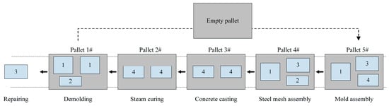
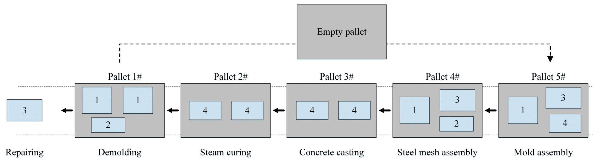
Figure 1 illustrates the workstation layout and process flow of a PC production line based on movable pallets. The production line is equipped with several circulating pallets, which are arranged according to the production process logic, including mold assembly, steel mesh assembly, concrete casting, steam curing, demolding, and component repair [42]. Each pallet can flexibly accommodate different types and quantities of PC components based on component dimensions and specifications. In the figure, different numbered PC components are arranged on each pallet, representing a grouping scheme of various components on a single pallet. Except for the PC repair process, the pallets carrying the components move along the process sequence in turn, and after completing all process steps, the finished products are output. After the demolding step, the empty pallets are returned to the mold assembly station for the next production cycle [43].

Figure 1. PC production line and its production processes.

In PC production planning, the primary challenge arises at the mold assembly stage, namely how to determine the optimal grouping scheme for components on pallets. Given a fixed number of PC components, the problem is how to rationally design the arrangement and combination of components on pallets so that the number of pallets required can be kept at a relatively low level while improving the utilization efficiency of spatial resources.

Another key task is the sequencing and scheduling optimization of pallets carrying PC components. Its purpose is to achieve a balance in delivery costs through reasonable scheduling arrangements, reducing both inventory holding costs caused by early completion and contractual penalties caused by delayed delivery. It is worth noting that a coupling relationship exists between grouping and scheduling. If the maximization of pallet space utilization is pursued alone, it may lead to imbalanced process workloads and increased waiting time on the production line. Conversely, if only scheduling optimization is considered, pallet space resources may remain idle. Therefore, it is necessary to optimize the two aspects in a coordinated manner.

3.2. Model Assumptions

1. All pallets used on the production line have identical specifications, effective working area, and rated load capacity. Pallet circulation time is negligible, and pallet failures, repairs, and abnormal conditions are not considered during the production cycle.

2. The geometric dimensions, weight, order affiliation, delivery date, and process requirements of all PC components to be produced are known and fixed parameters.

3. Production standards for components are uniform, and no component scrapping or rework occurs during production.

4. The processing time for a single component in each process is a fixed constant. The processing time for each pallet in each process is equal to the sum of the processing times of all components it holds in that process.

5. Workstations operate sequentially; a single workstation can process only one pallet at a time, and a single pallet can only be processed at one workstation at a time.

6. The buffer area between processes on the production line has sufficient capacity, preventing production blockage due to work-in-process accumulation.

7. Early completion of components incurs unit-time inventory storage costs, while delayed delivery incurs unit-time penalty costs. Both cost coefficients are known and fixed values [22,41].

8. The model only covers the production process and does not consider the additional costs of finished product transportation, off-site warehousing, and batch delivery.

3.3. Mathematical Model of PC-GS

All notations in the model are detailed in the Notations. In the PC mold assembly process, the grouping of PC components on pallets is subject to the following constraints:

$${\displaystyle \sum _{j\in J}{c}_{\mathit{ktj}}}=1,\hspace{1em}\forall (k,t)\in I$$

(1)

$$c_{\mathit{ktj}}\le y_j,\hspace{1em}\forall (k,t)\in I,j\in J$$

(2)

$$a_{\mathit{ktj}}\ge e\cdot c_{\mathit{ktj}},\hspace{1em}\forall (k,t)\in I,j\in J$$

(3)

$$b_{\mathit{ktj}}\ge e\cdot c_{\mathit{ktj}},\hspace{1em}\forall (k,t)\in I,j\in J$$

(4)

$$a_{\mathit{ktj}}+w_k\left(1-r_{\mathit{kt}}\right)+h_k{r}_{\mathit{kt}}\le \left(W-e\right)+M_W\cdot \left(1-c_{\mathit{ktj}}\right),\hspace{1em}\forall (k,t)\in I,j\in J,M_W=W$$

(5)

$$b_{\mathit{ktj}}+h_k\left(1-r_{\mathit{kt}}\right)+w_k{r}_{\mathit{kt}}\le \left(H-e\right)+M_H\cdot \left(1-c_{\mathit{ktj}}\right),\hspace{1em}\forall (k,t)\in I,j\in J,M_H=H$$

(6)

$$a_{\mathit{ktj}}+w_k\left(1-r_{\mathit{kt}}\right)+h_k{r}_{\mathit{kt}}+e\le a_{\mathit{lsj}}+M_W\cdot \left(1-u_{\mathit{kt},\mathit{ls},j}^L\right),\hspace{1em}\forall (k,t)<(l,s)\in I,j\in J,M_W=W$$

(7)

$$a_{\mathit{lsj}}+w_l\left(1-r_{\mathit{ls}}\right)+h_l{r}_{\mathit{ls}}+e\le a_{\mathit{ktj}}+M_W\cdot \left(1-u_{\mathit{kt},\mathit{ls},j}^R\right),\hspace{1em}\forall (k,t)<(l,s)\in I,j\in J,M_W=W$$

(8)

$$b_{\mathit{ktj}}+h_k\left(1-r_{\mathit{kt}}\right)+w_k{r}_{\mathit{kt}}+e\le b_{\mathit{lsj}}+M_H\cdot \left(1-v_{\mathit{kt},\mathit{ls},j}^B\right),\hspace{1em}\forall (k,t)<(l,s)\in I,j\in J,M_H=H$$

(9)

$$b_{\mathit{lsj}}+h_l\left(1-r_{\mathit{ls}}\right)+w_l{r}_{\mathit{ls}}+e\le b_{\mathit{ktj}}+M_H\cdot \left(1-v_{\mathit{kt},\mathit{ls},j}^A\right),\hspace{1em}\forall (k,t)<(l,s)\in I,j\in J,M_H=H$$

(10)

$$u_{\mathit{kt},\mathit{ls},j}^L+u_{\mathit{kt},\mathit{ls},j}^R+v_{\mathit{kt},\mathit{ls},j}^B+v_{\mathit{kt},\mathit{ls},j}^A\ge c_{\mathit{ktj}}+c_{\mathit{lsj}}-1,\hspace{1em}\forall (k,t)<(l,s)\in I,j\in J$$

(11)

$${\displaystyle \sum _{t=1}^{m_k}{U}_{\mathit{kt}}}(u)\le Q_k,\hspace{1em}\forall k\in K,\forall t\ge 0$$

(12)

$$y_j,c_{\mathit{ktj}},r_{\mathit{kt}},u_{\mathit{kt},\mathit{ls},j}^L,u_{\mathit{kt},\mathit{ls},j}^R,v_{\mathit{kt},\mathit{ls},j}^B,v_{\mathit{kt},\mathit{ls},j}^A\in \{0,1\}$$

(13)

$$a_{\mathit{ktj}}\ge 0,\hspace{1em}{b}_{\mathit{ktj}}\ge 0,\hspace{1em}\forall (k,t)\in I,j\in J$$

(14)

Equation (1) denotes that the mold of each PC component must be placed on exactly one pallet. Equation (2) denotes that a pallet must be activated if any PC is placed in it; no PC can be placed in an unused pallet. Equations (3)–(6) respectively require a minimum gap of e between the left, bottom, right, and top edges of each PC and the corresponding pallet edges. When two PC components are placed on the same pallet, they are required to satisfy both non-overlap and minimum production gap constraints. Equations (7) and (8) describe the positional coordinate relationships for the case where any two components are in a left-right adjacent configuration, ensuring non-overlap and minimum spacing. Equations (9) and (10) describe the coordinate constraints for a top-bottom separated configuration. The big-M parameters M_W and M_H in Equations (5)–(10) are both related to the coordinates of the PC components on the pallet, and their relatively tight values do not exceed the pallet dimensions. Therefore, M_W and M_H can be set to the pallet width and height, respectively. Equation (11) expresses the mutual positional logic constraint, which states that for any two components on the same pallet, at least one type of separation with gap must be satisfied. Equation (12) indicates that the quantity of each PC mold type used per use does not exceed its prepared inventory. Equations (13) and (14) represent the variable domain constraints.

After the molds of PC components are grouped and placed onto pallets, they proceed sequentially through the following processes: steel mesh assembly, concrete casting, steam curing, demolding, and component repair. In this process, the pallets carrying PC components are equivalent to jobs in the production scheduling problem, where the objective is to determine at which workstation each job is processed. The following constraints must be satisfied:

$$C_{\mathit{jp}}\le S_{j,p+1},\hspace{1em}\forall j\in J,p=1,2,3,4,5$$

(15)

$${\displaystyle \sum _{q\in M_p}{x}_{\mathit{jpq}}}=1,\hspace{1em}\forall j\in J,\forall p\in P$$

(16)

$$C_{j6}\le C_{\max },\hspace{1em}\forall j\in J$$

(17)

$$t_{\mathit{jp}}=\left\{\begin{array}{c}{\displaystyle \sum _{k\in K}\left({\displaystyle \sum _{t=1}^{m_k}{c}_{\mathit{tkj}}}\right)}\cdot x_{\mathit{kp}},\hspace{1em}\hspace{1em}\hspace{1em}\forall j\in J,p\in \{1,2,3,5,6\}\\ t^{*},\hspace{1em}\hspace{1em}\hspace{1em}\forall j\in J,p=4\end{array}\right.$$

(18)

$${\displaystyle \sum _{d\in D}{t}_{\mathit{jpd}}}=t_{\mathit{jp}},\hspace{1em}\forall j\in J$$

(19)

$$\begin{array}{cc}\begin{array}{r}\hfill \mathit{WS}(d)\le S_{\mathit{jpd}}\le C_{\mathit{jpd}}\le \mathit{WN}(d)\\ \hfill C_{\mathit{jpd}}-S_{\mathit{jpd}}=t_{\mathit{jpd}}\\ \hfill 0\le t_{\mathit{jpd}}\le H_w\cdot y_{\mathit{jpd}}\end{array}& \forall j\in J,\forall d\in D\end{array}$$

(20)

$$\begin{array}{cc}\begin{array}{r}\hfill S_{\mathit{jp}}\le S_{\mathit{jpd}}\\ \hfill C_{\mathit{jp}}\ge C_{\mathit{jpd}}\\ \hfill C_{\mathit{jpd}}\le S_{\mathit{jp},d+1}\end{array}& \forall j\in J,\forall d\in D,d<D_{\max }\end{array}$$

(21)

$$\begin{array}{cc}\begin{array}{c}{S}_{\mathit{jpd}}\ge C_{j^{\prime }\mathit{pd}}-H_w\cdot \left(2-x_{\mathit{jpd}}-x_{j^{\prime }\mathit{pd}}\right)-H_w\cdot \left(2-y_{\mathit{jpd}}-y_{j^{\prime }\mathit{pd}}\right)\\ S_{j^{\prime }\mathit{pd}}\ge C_{\mathit{jpd}}-H_w\cdot \left(2-x_{\mathit{jpd}}-x_{j^{\prime }\mathit{pd}}\right)-H_w\cdot \left(2-y_{\mathit{jpd}}-y_{j^{\prime }\mathit{pd}}\right)\end{array}& \forall j,j^{\prime }\in J,j\ne j^{\prime },\forall p\in M_p,\forall d\in D\end{array}$$

(22)

$${\displaystyle \sum _{j\in J}{t}_{\mathit{jpd}}}\cdot x_{\mathit{jpq}}\le H_w,\hspace{1em}\forall q\in M_p,\forall d\in D$$

(23)

$${\displaystyle \sum _{d\in D}{z}_{j3d}}=1,\hspace{1em}j\in J$$

(24)

$$\begin{array}{cc}\begin{array}{l}{S}_{j3}\ge \mathit{WS}(d)-M_T\cdot \left(1-z_{j3d}\right)\hspace{1em}\hspace{1em}\hfill \\ C_{j3}\le \mathit{WE}(d)+M_T\cdot \left(1-z_{j3d}\right)\hfill \end{array}& \forall j\in J,\forall d\in D\end{array}$$

(25)

$$C_{j3}=S_{j3}+t_{j3},\hspace{1em}\forall j\in J$$

(26)

$$\begin{array}{cc}\begin{array}{l}{S}_{j3}\ge C_{j^{\prime }3}-\left(H_w+H_a\right)\cdot \left(2-z_{j3d}-z_{j^{\prime }3d}\right)-\left(H_w+H_a\right)\cdot \left(2-x_{j3q}-x_{i^{\prime }3q}\right)\hfill \\ S_{j^{\prime }3}\ge C_{j3}-\left(H_w+H_a\right)\cdot \left(2-z_{j3d}-z_{j^{\prime }3d}\right)-\left(H_w+H_a\right)\cdot \left(2-x_{j3q}-x_{i^{\prime }3q}\right)\hfill \end{array}& \forall j,j^{\prime }\in J,j\ne j^{\prime },\forall p\in M_3,\forall d\in D\end{array}$$

(27)

$${\displaystyle \sum _{j\in J}{t}_{j3}}\cdot x_{j3q}\cdot z_{j3d}\le H_w+H_a,\hspace{1em}\forall q\in M_3,\forall d\in D$$

(28)

$${\displaystyle \sum _{d\in D}{z}_{j4d}}=1,\hspace{1em}\forall j\in J$$

(29)

$$\begin{array}{cc}\begin{array}{c}{S}_{j4}\ge \mathit{WS}(d)-M_T\cdot \left(1-z_{j4d}\right)\\ S_{j4}\le \mathit{WE}(d)+M_T\cdot \left(1-z_{j4d}\right)\end{array}& \forall j\in J,\forall d\in D\end{array}$$

(30)

$$C_{j4}^{\prime }=S_{j4}+t_{j4},\hspace{1em}\forall j\in J$$

(31)

$$C_{j4}\ge C_{j4}^{\prime },\hspace{1em}\forall j\in J$$

(32)

$$\begin{array}{cc}\begin{array}{c}{S}_{j4}\ge C_{j^{\prime }4}^{\prime }-M_T\cdot \left(2-x_{j4k}-x_{j^{\prime }4q}\right)\\ S_{j^{\prime }4}\ge C_{j4}^{\prime }-M_T\cdot \left(2-x_{j4k}-x_{j^{\prime }4q}\right)\end{array}& \forall j,j^{\prime }\in J,j\ne j^{\prime },\forall q\in M_4\end{array}$$

(33)

$$t_{\mathit{jp}},S_{\mathit{jp}},C_{\mathit{jp}},C_{j4}^{\prime },S_{\mathit{jpd}},C_{\mathit{jpd}},t_{\mathit{jpd}},C_{\max }\ge 0$$

(34)

$$x_{\mathit{jpq}},y_{\mathit{jpd}},z_{j3d},z_{j4d}\in \{0,1\}$$

(35)

Equation (15) denotes the process sequence constraint that the next process can only start after the previous process is completed. Equation (16) denotes that each job must be assigned to exactly one parallel machine per process. Equation (17) expresses the makespan constraint. Equation (18) indicates that in the curing stage, the processing time of pallets carrying PC elements equals a fixed value t^*, while the processing time in other stages is the sum of the processing times of components on the pallet for each stage. For the mold assembly, steel mesh assembly, demolding, and PC repairing processes, they are subject to interruptible operation constraints [6,12]. If the work cannot be completed within the normal working hours of the current day, the operation may be suspended midway and resumed on the next working day. Equations (19)–(23) express these interruptible operation constraints. Equation (19) indicates that the sum of daily processing durations equals the total net processing time of the interruptible jobs. Equation (20) states the daily working window constraint that the operation only occurs during regular working hours, no overtime allowed. Equation (21) performs the coordinate transformation from the continuous global time of the schedule to the workday index and the relative time within the day. This transformation is used to accommodate the time rule determinations for daily work, overtime, and interruptible operations across processes. Constraint (22) uses the big-M method to ensure that, on the same machine and within the same working day, the processing time intervals of any two jobs do not overlap. Equation (23) restricts the cumulative processing time (including waiting time) of all jobs on a single machine within the same working day to not exceed the maximum allowable time window of that stage for that day.

The casting stage is a non-interruptible process. Meanwhile, to improve production efficiency and make full use of non-working time, the casting stage can be completed with appropriate overtime. Equation (24) indicates that the casting operation is required to be completed within a single working day and cannot be split. Equation (25) represents the single-day time window constraint for the casting process, meaning that its entire processing duration falls within the normal working hours and overtime hours of that day. Equation (26) represents the non-interruptible continuous processing constraint for the casting process. Equations (27) and (28) respectively represent the non-overlap constraint for parallel machines on a single day and the machine daily load constraint for the casting process.

The curing stage is a non-interruptible parallel processing stage. It allows processing to continue across multiple working days without being truncated by daily time windows. Equation (29) indicates that the start time of the curing stage must fall within the normal working and overtime hours of a working day. Equation (30) states that once the steam curing operation starts, it cannot be interrupted; it may continue across working days and is not forced to stop due to daily shift ends. Equation (31) describes that the curing equipment operates automatically and continuously, and may span non-working periods. Equation (32) indicates that the effective completion time of the curing stage is not earlier than its actual completion time; if completion occurs during non-working hours, it is automatically deferred to the start of the next working day. Equation (33) indicates that a single curing device cannot process two jobs simultaneously within the same time period. Equations (34) and (35) represent the variable domain constraints. It should be noted that the big-M parameter in the time scheduling stage can be determined by ten times the required due date of the PC order.

Based on the above constraints, this study simultaneously optimizes three objectives. Equation (36) aims to minimize the number of pallets used; a smaller value indicates higher pallet utilization efficiency. Equation (37) denotes the minimization of the makespan. Equation (38) is used to minimize the temporary storage cost caused by early completion of PC components and the contractual penalty cost resulting from delayed delivery.

$$\min f_1={\displaystyle \sum _{j\in J}{y}_j}$$

(36)

$$\min f_2=C_{\mathit{max}}$$

(37)

$$\min f_3={\displaystyle \sum _{k\in K}{\displaystyle {\sum }_{t=1}^{m_k}\left(a\cdot \mathit{max}\left\{0,d_k-e_{\mathit{kt}}\right\}+b\cdot \mathit{max}\left\{0,e_k-d_{\mathit{kt}}\right\}\right)}}$$

(38)

4. QL-NSGA-II for PC-GS

4.1. Advantages of the QL-NSGA-II Algorithm

The joint optimization of grouping and scheduling in PC production is a strongly NP-hard problem [10]. The solution space includes not only discrete combinations of component spatial layouts but also complex continuous-time scheduling constraints. When solving such high-dimensional, strongly coupled problems, conventional NSGA-II typically uses fixed crossover and mutation rates and relies on a single grouping heuristic. Such static parameter settings can cause the algorithm to become trapped in local optima during evolution, a phenomenon often described as premature convergence, or to lack refined local search capability in the later stages of evolution.

To address these limitations, this paper proposes a hybrid algorithm that combines Q-learning and NSGA-II, referred to as QL-NSGA-II. The main advantage of this algorithm lies in a two-level control architecture that connects a reinforcement learning agent with the genetic evolution environment. The Q-learning module functions as a meta-controller and does not require prior knowledge of the underlying complex physical constraints of the system [44]. Instead, it monitors the hypervolume variation in the population during the iterative process and dynamically learns to assign the most suitable grouping heuristic rule and genetic operator combination. This data-driven adaptive mechanism helps the algorithm maintain a better balance between global exploration and local exploitation.

4.2. Chromosome Encoding and Decoding

4.2.1. Encoding Scheme

In PC production, grouping is used to address the spatial layout of components on the demolding platform, while scheduling aims to solve the sequencing problem of pallets that carry the components. Since both problems focus on PC components as the research object, a two-level segmented real vector encoding strategy is adopted in QL-NSGA-II to integrate the spatial grouping decisions of components and the temporal scheduling decisions of the workshop within a single chromosome.

The first layer of the encoding represents the components themselves. Given the limited supply of precast concrete molds, the first-layer chromosome is divided into several batches. For example, there are 13 PC components of four types in Figure 2. Except for the first type, whose mold supply is 1, the mold supply for all other types is 2. Consequently, only 7 components can be encoded in the first batch, while the remaining 6 components are encoded in the second batch. The second layer represents the placement orientation of the precast concrete components on the demolding platform, where 0 indicates horizontal placement and 1 indicates placement after orthogonal rotation.

Figure 2. A feasible encoding scheme.

4.2.2. Decoding Strategy

The decoding process consists of two steps. The first step is to assign components in the encoding to pallets, a process also referred to as the grouping strategy. This step determines the number of pallets that are activated. To address the heterogeneity in the size distribution of components, three decoding heuristic rules with complementary characteristics are constructed.

Subsequently, the pallets carrying the components are treated as independent jobs. By combining the processing time of each component type at each operation, the actual processing time of each pallet at each operation can be obtained. It should be noted that the steam curing operation is independent of the number of components on the pallet, and its processing time generally depends on the curing process requirements of the concrete components. For simplicity of calculation, it is set as a fixed value. Finally, the pallets are assigned to the machines of the corresponding operations according to the first-come first-service in the hybrid flow shop scheduling strategy, so that the maximum completion time and the penalty cost can be calculated.

4.2.3. Genetic Operators

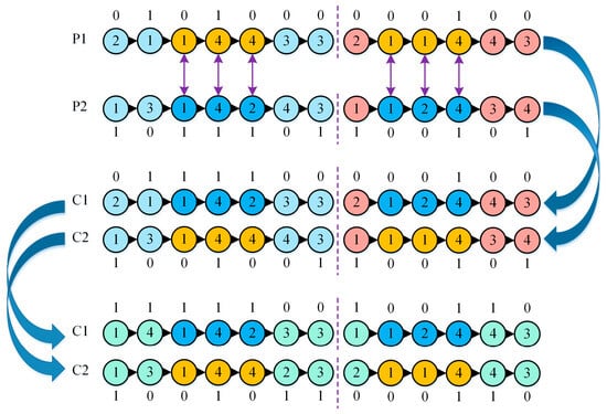
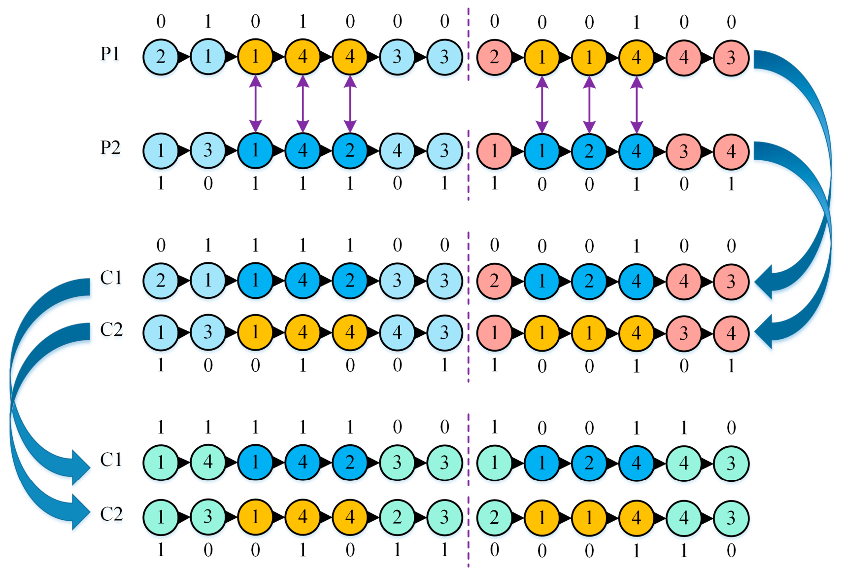
Under the proposed dual-layer encoding framework, the algorithm’s genetic operations consist of two core steps: two-point crossover and two-point mutation. In the two-point crossover operation, as shown in Figure 3, the algorithm randomly selects two identical crossover points within the gene sequences of two parent individuals (P1 and P2). It then entirely swaps the genetic segments between these two points to generate the initial offspring (C1 and C2). To resolve the issues of duplicated or missing component IDs that may arise after crossover, the algorithm employs a repair strategy based on partially mapped crossover. This strategy replaces redundant genes outside the crossover region with the missing valid genes, thereby maintaining the physical legality of the operation sequence while preserving the excellent traits of the parents.

Figure 3. Crossover operator.

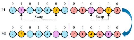
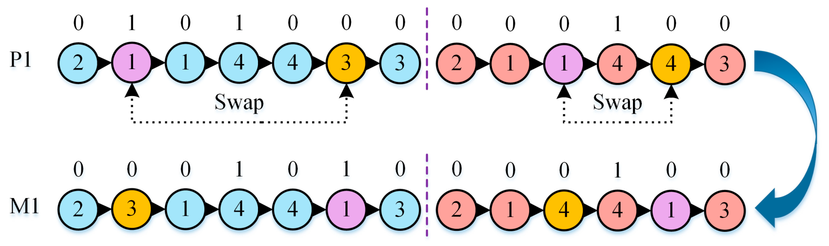
The two-point mutation operation in Figure 4 injects random perturbations into the population, helping the algorithm escape local optima. This operation acts on a single parent individual (P1). The algorithm then selects two random mutation points in the sequence and directly swaps the component gene blocks at those positions.

Figure 4. Mutation operator.

4.3. Process Design Based on Q-Learning

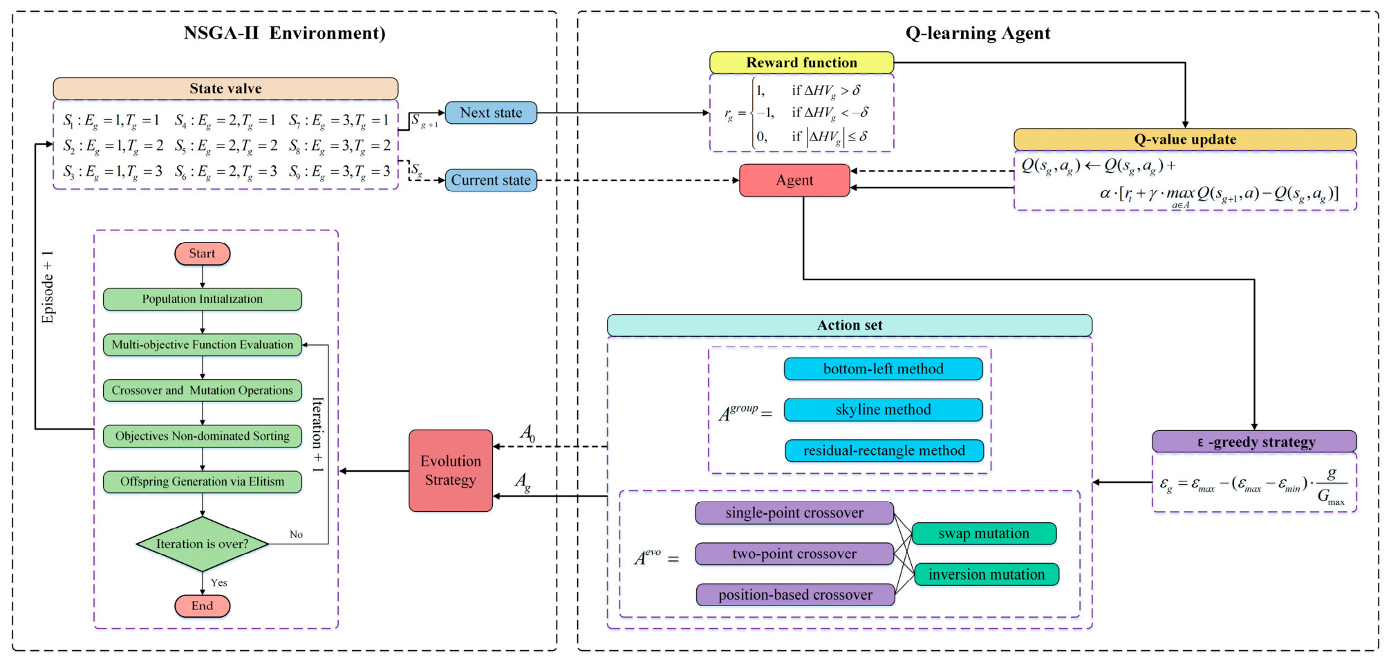
In this study, a Q-learning reinforcement learning mechanism is introduced as a meta-controller and embedded into the evolutionary loop of NSGA-II. Through a Markov decision process, this controller continuously interacts with the evolutionary environment to achieve dynamic and adaptive regulation of the underlying operators [39,45]. Its core components include the state space, the action space, the reward function, and the update strategy. The specific definitions are as follows.

4.3.1. State Space

Based on the population evolution characteristics of NSGA-II, this paper constructs a compact two-dimensional discrete state space S. At any generation g, the system state S_g in S is uniquely determined by two feature dimensions. The first dimension is the evolution stage. NSGA-II has different demands for global exploration and local exploitation at different search stages. By using the ratio of the current generation g to the maximum generation G_max, the search process is divided into three stages, namely the early stage, the middle stage, and the late stage, as defined in Equation (39). Here, E_g ∈ {1,2,3}, and ⌈⋅⌉ denotes the ceiling function.

$$E_g=⌈3\cdot {\displaystyle \frac{g}{G_{\max }}}⌉\hspace{1em}\hspace{1em}\hspace{1em}\hspace{1em}\forall g\in G$$

(39)

The second dimension is the population quality trend, which is used to characterize the evolutionary vitality of the population in the objective space. The trend is determined by calculating the difference between the true hypervolume (HV) values of the population in the two most recent generations, as shown in Equation (40). Here, T_g represents the population quality being in an improving state, a stagnant state, or a deteriorating state, and δ is a preset small positive threshold. Combining the above two dimensions, the state space contains nine discrete states.

$$T_g=\left\{\begin{array}{ll}1,\hfill & \mathrm{if}\Delta H{V}_g>\mathit{\delta }\hfill \\ 2,\hfill & \mathrm{if}\left|\Delta H{V}_g\right|\le \mathit{\delta }\hfill \\ 3,\hfill & \mathrm{if}\Delta H{V}_g<-\mathit{\delta }\hfill \end{array}\right.\forall g\in G,\Delta H{V}_g=H{V}_g-H{V}_{g-1}$$

(40)

4.3.2. Action Space

To address the decoupling requirement between the spatial grouping constraints and the scheduling time constraints for PC components, we design a dual-action space mechanism comprising a grouping-mapping strategy (grouping action space, A^group) and a genetic evolution strategy (genetic action space, A^veo). At each state transition, the agent must simultaneously output decision instructions for both action spaces.

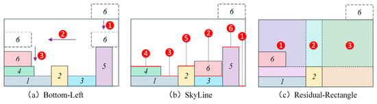
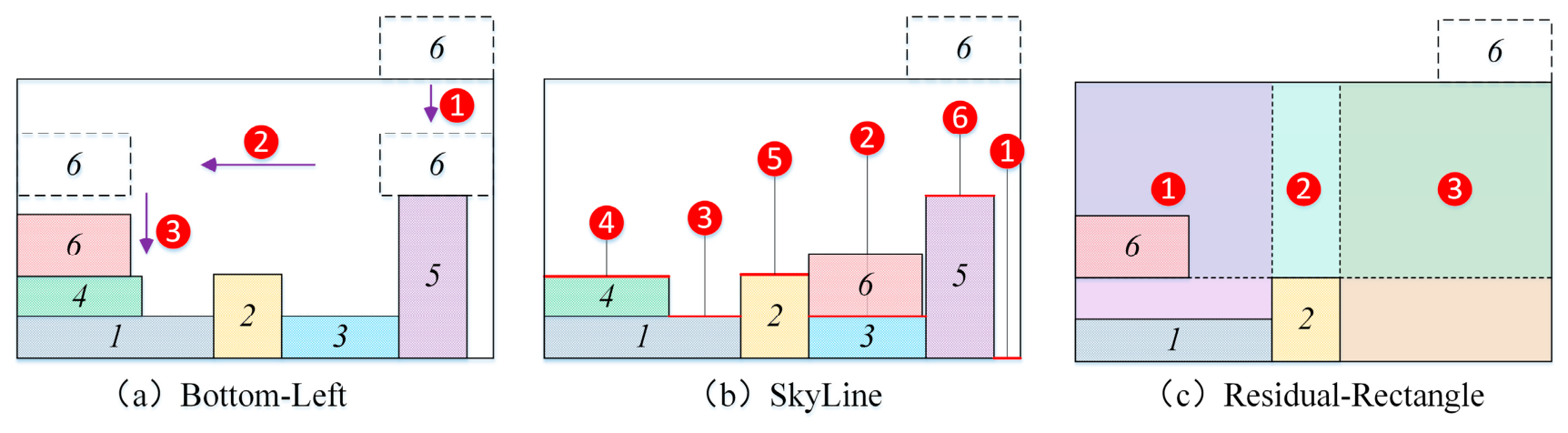
The grouping action space provides three methods for placing PC component molds onto pallets, which the agent can dynamically invoke according to the population evolution state. The first is the bottom-left method, which relies on a successive translation rule that moves downward, then leftward, then downward again, forcing the component to be placed in the lowest and leftmost available area on the current pallet. The second is the skyline method, which dynamically tracks the stepped contour formed by the tops of already arranged components on the pallet, directly extracting horizontal line segments as candidate placement reference points. This approach helps maintain local packing compactness while effectively reducing the optimization dimension and computational cost. The last is the residual-rectangle method, which dynamically partitions and updates all unoccupied free areas inside the pallet into two-dimensional rectangular blocks, thereby capturing and filling fragmented idle spaces. Figure 5 illustrates the schematic process of the three actions in the grouping action space.

$$A^{\mathit{group}}=\{a_1^{\mathit{group}},a_2^{\mathit{group}},a_3^{\mathit{group}}\}$$

(41)

Figure 5. Process of the three actions in the grouping action space.

To reduce the dimensionality of the action space, the evolutionary action space is constructed with three crossover strategies and two mutation methods. The crossover strategies include single-point, two-point, and position-based crossovers, while the mutation strategies include swap and inversion mutations. Two-point crossover and swap mutation are detailed in Section 4.2. The orthogonal combination of these strategies yields six discrete actions that together form a complete spectrum ranging from local exploitation to global exploration.

$$A^{\mathit{evo}}=\{a_1^{\mathit{evo}},a_2^{\mathit{evo}},a_3^{\mathit{evo}},a_4^{\mathit{evo}},a_5^{\mathit{evo}},a_6^{\mathit{evo}}\}$$

(42)

4.3.3. Hypervolume-Based Reward Function

The grouping and scheduling optimization of PC components involves three objectives with significantly different scales: the number of pallets, the makespan, and the penalty cost. Traditional reward mechanisms based on a single scalar fitness often lead to distorted evaluation. Therefore, this paper designs a HV-based reward function as the sole feedback signal to guide the agent’s learning. The mechanism first uses the global ideal point to dynamically normalize the first non-dominated front of the current evolutionary generation, and then calculates the Lebesgue measure formed by the solution set of that front together with a reference point in the multi-objective space to obtain the HV [39]. By comparing the difference in HV between two successive generations, the reward function is obtained as shown in Equation (43).

$$r_g=\left\{\begin{array}{ll}1,\hfill & \mathrm{if}\Delta H{V}_g>\mathit{\delta }\hfill \\ -1,\hfill & \mathrm{if}\Delta H{V}_g<-\mathit{\delta }\hfill \\ 0,\hfill & \mathrm{if}\left|\Delta H{V}_g\right|\le \mathit{\delta }\hfill \end{array}\right.\hspace{1em}\hspace{1em}\hspace{1em}\forall g\in G,\Delta H{V}_g=H{V}_g-H{V}_{g-1}$$

(43)

4.3.4. Action Selection and Q-Value Update

In the dual-layer control architecture of QL-NSGA-II, the agent maintains separate grouping and evolutionary Q-tables, denoted as Q^group and Q^evo, to record the expected cumulative returns of various operator combinations under different states. To achieve a favorable balance between exploration of unknown strategies and exploitation of known optimal strategies, the agent adopts a dynamically decaying ε-greedy policy for both the grouping and evolutionary action spaces. At the evolutionary state S_g of generation g, the decision rule for the agent to select action a_g is given by Equation (44).

$$a=\left\{\begin{array}{l}\mathit{arg}\underset{a\in A}{\mathit{max}}Q(s_g,a),\hspace{1em}\hspace{1em}{\epsilon }_g\le \mathit{prob}<1\hfill \\ \mathit{random}\mathit{select}a\mathit{in}A,\hspace{1em}\hspace{1em}0<\mathit{prob}<{\epsilon }_g\hfill \end{array}\right.$$

(44)

The equation shows that the agent performs exploitation with a high probability of 1 − ε_g, that is, it directly queries the Q-tables and selects the action with the highest expected value under the current state. At the same time, it retains a probability of ε_g to perform uniform random sampling in the action space A. To enable broad trial-and-error capability in the early stages of evolution, while ensuring stable convergence to the optimal operator in the later stages, the exploration rate ε_g decays linearly with the evolutionary generation g. In Equation (44), ε_max and ε_min denote the initial upper and lower bounds of the exploration rate, respectively, and G_max is the maximum number of evolutionary generations.

$${\epsilon }_g={\epsilon }_{\mathit{max}}-({\epsilon }_{\mathit{max}}-{\epsilon }_{\mathit{min}})\cdot {\displaystyle \frac{g}{G_{\max }}}\hspace{1em}\hspace{1em}\forall g\in G$$

(45)

After the agent issues the action instructions ($a_g^{\mathit{group}},a_g^{\mathit{evo}}$) at state S_g, the underlying NSGA-II performs decoding of the physical environment and population evolution. Subsequently, the system observes the transition to a new state S_g+1 and computes a HV-based immediate reward r_g. Based on the off-policy mechanism, the agent updates the corresponding value elements in the Q-tables using the Bellman equation.

$$Q(s_g,a_g)\leftarrow Q(s_g,a_g)+\alpha \cdot [r_t+\gamma \cdot \underset{a\in A}{\mathit{max}}Q(s_{g+1},a)-Q(s_g,a_g)]$$

(46)

In Equation (46), α ∈ (0, 1] is the learning rate, which controls the extent to which newly acquired reward information adjusts the historical estimates. γ ∈ [0, 1) is the discount factor, which quantifies the weight of future potential rewards in the current decision [39].

4.4. Overall Algorithm Workflow

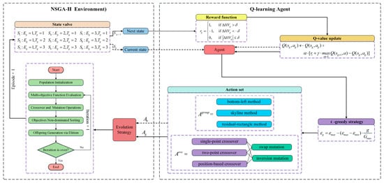
The QL-NSGA-II algorithm decouples the PC component grouping and scheduling process into two parts: agent decision-making and environment evolution. The detailed procedure is illustrated in Figure 6.

Figure 6. Flowchart of the QL-NSGA-II.

In the agent decision-making part, the Q-learning agent acts as a controller. It extracts the current generation progress and the HV difference in the population to perceive the discrete evolutionary state. Through a dynamically decaying ε-greedy policy, it independently makes decisions from the Q-tables and issues the grouping rule and evolutionary operator combination strategy. In the environment evolution part, the NSGA-II environment receives the instructions, invokes the corresponding genetic operators to perform population reproduction and decoding, and calculates the multi-objective fitness values. After environmental selection, the system computes the HV change in the new Pareto front, converts it into a discrete reward, and feeds it back to the agent. This drives the Bellman equation to update the value system, ultimately guiding the algorithm to adaptively converge to the global optimal solution set.

5. Experimental Study and Analysis

To thoroughly evaluate the performance of the proposed QL-NSGA-II in solving the PC-GS, all comparative experiments are conducted on a unified software and hardware platform. The hardware environment includes an Intel Core i5-10500 processor at 3.1 GHz, 16.0 GB of RAM, and the Windows 10 operating system. The software environment is based on the MATLAB R2022b computing platform.

5.1. Experimental Setup and Parameters

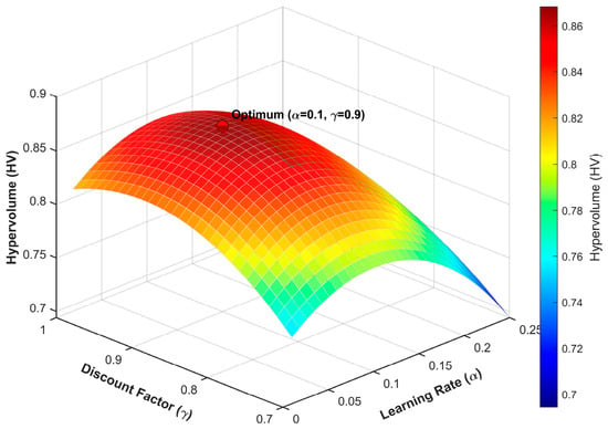
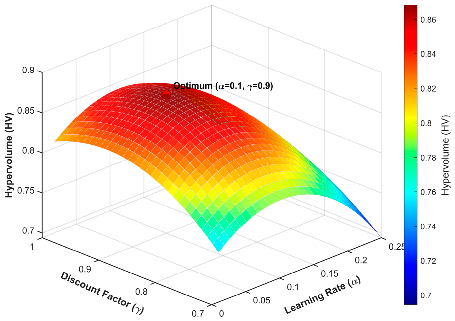
The test instances consist of two types. The first type includes three benchmark instances, denoted as P10 [46], P20 [22], and P30 [46], which are taken from published literature. These instances are used to verify the algorithm’s optimization capability on the boundaries of single-objective extrema. The second type comprises real production orders extracted from a large prefabricated construction component factory in Zigong, Sichuan Province of China. Before conducting the formal experiments, a grid search pre-experiment was performed on the two core coupled hyperparameters of Q-learning, namely the learning rate and the discount factor. The final global optimal parameters are shown in Figure 7.

Figure 7. Sensitivity analysis for core Q-learning hyperparameters of $\mathsf{\alpha }$ and $\mathsf{\gamma }$.

The parameters of the environment-level NSGA-II, such as population size and maximum evolutionary generation, are kept consistent with those in the literature. The parameters of the agent control layer are set as follows: the maximum number of training episodes E_max is 100, the learning rate $\mathsf{\alpha }$ is 0.1, the discount factor $\mathsf{\gamma }$ is 0.9, the upper and lower bounds of the exploration rate ${\mathsf{\epsilon }}_{\mathit{max}}$ and ${\mathsf{\epsilon }}_{\mathit{min}}$ are 0.9 and 0.1, respectively, and the reward minimum threshold δ is 10⁻⁴.

5.2. Benchmark Instances

As shown in Table 1, the QL-NSGA-II algorithm demonstrates good optimization stability on benchmark instances from the literature with different scales and machine configurations. For the P10 instance and the P20 with the first parallel machine configuration, the makespan and penalty cost obtained by our algorithm are consistent with the benchmark solutions provided in the existing literature. This indicates that, under the framework of multi-objective joint scheduling, the algorithm still retains a single-objective boundary optimization capability comparable to that of the existing benchmark algorithms.

Table 1. Comparison of QL-NSGA-II with known optimal solutions on benchmark instances.

Case	Machine Configuration	Optimization Objective	Literature Algorithms	QL-NSGA-II	Relative Deviation
P10 [46]	1,1,1,10,1,1	Cmax (hour)	126.9	126.9	0.00%
		Penalty cost (yuan)	701.6	701.6	0.00%
P20 [22]	1,1,1,8,1,1	Cmax (hour)	236.3	236.3	0.00%
		Penalty cost (yuan)	31.92	31.92	0.00%
P20 [22]	2,3,1,8,1,1	Cmax (hour)	48.64	31.73	↓ 34.77%
		Penalty cost (yuan)	443.84	176.48	↓ 60.24%
P30 [46]	1,1,1,10,1,1	Cmax (hour)	315.1	219.1	↓ 30.47%
		Penalty cost (yuan)	2525.9	2204.1	↓ 12.74%

Note: Optimal solutions by QL-NSGA-II on P20: 11-1-15-5-9-3-4-2-7-12-8-13-10-6-18-19-14-16-20-17; Optimal solutions by QL-NSGA-II on P30: 10-4-4-4-4-4-9-1-1-3-2-1-1-2-3-9-9-6-6-9-8-8-7-9-6-7-5-5-5-10.

When the machine configuration becomes more complex or the problem scale increases, QL-NSGA-II shows certain performance advantages. For the P20 instance with the parallel machine configuration (2,3,1,8,1,1), the makespan obtained by our algorithm is reduced from the benchmark value of 48.64 h to 31.73 h, which is a reduction of 34.77% compared with the optimal solution in the literature, while the penalty cost is reduced by 60.24%. For the P30 instance, the makespan and penalty cost are also reduced by 30.47% and 12.74%, respectively, compared with the literature solutions.

In addition, to facilitate comparison and verification of the computational results, the optimal scheduling sequences corresponding to the P20 and P30 instances obtained by our algorithm are specifically listed below the table. This performance disparity stems from the limited solution space of simple instances, where benchmark algorithms can already converge to the global optimum. In contrast, the solution space of complex instances expands exponentially, making traditional algorithms prone to local optima, whereas the proposed algorithm’s reinforcement-learning dynamic search mechanism can better leverage its optimization strengths and obtain higher-quality feasible solutions.

5.3. Real Production Case

The test data for case P87 in Table 2 are derived from real production orders of composite slabs from a prefabricated construction enterprise in Zigong, China. This batch scheduling task involves 21 types of precast components with varying specifications, and the total demand is 87 units. The demand quantity and the available mold inventory vary for each component type. For example, PC type 1# has a demand of 2 units, while the corresponding mold quantity is also 2. In this case, the molds need to be reused twice to fulfill the order. The physical dimensions of these components exhibit a relatively noticeable distribution, with lengths ranging from 1500 mm to 5920 mm and widths ranging from 1020 mm to 2620 mm. To meet the just-in-time delivery requirements of the construction site, each component of each type is assigned a precise, independent due time. For example, there are eight units of PC type 2#, among which two units have a required time of 1872 min, two units have 7344 min, two units have 8784 min, and the remaining units have other due times.

Table 2. Real PC production order information for P87.

PC	Mold Number	Order Demand	Size (mm)		Due Date	Process Time (min)
			Length	Width	Due Time × Nuber (min × piece)	P1	P2	P3	P4	P5	P6
1#	2	4	2920	2360	1872 × 1/3168 × 1/4464 × 1/5904 × 1	22	24	17	420	18	12
2#	2	8	3520	1620	1872 × 2/4752 × 1/5760 × 1/7344 × 2/8784 × 2	22	22	16	420	18	11
3#	2	4	2520	1190	1728 × 2/4752 × 1/6048 × 1	15	18	13	420	15	10
4#	1	2	2520	2520	1872 × 1/5904 × 1	21	23	16	420	17	11
5#	2	7	3120	1710	3168 × 2/4752 × 2/7344 × 1/7488 × 1/8784 × 1	20	22	15	420	17	11
6#	3	8	3520	2360	1872 × 1/3024 × 2/4608 × 1/5760 × 1/5904 × 1/6048 × 1/7488 × 1	25	27	18	420	19	12
7#	1	2	5920	1920	1728 × 1/4464 × 1	34	32	20	420	22	13
8#	2	4	3310	1320	3024 × 1/3168 × 1/4752 × 1/5904 × 1	19	20	14	420	17	11
9#	2	4	3420	2000	3024 × 1/3168 × 1/4608 × 2	23	24	17	420	18	12
10#	3	5	3420	1220	1728 × 2/1872 × 1/4464 × 1/5904 × 1	19	20	14	420	17	10
11#	2	4	4320	2620	1728 × 1/3168 × 1/4464 × 1/6048 × 1	30	32	20	420	20	13
12#	2	4	1920	1220	1728 × 1/3168 × 1/4608 × 1/4752 × 1	12	16	13	420	14	10
13#	2	8	2920	1800	1728 × 2/4464 × 1/5904 × 1/7488 × 2/8784 × 2	20	22	15	420	17	11
14#	1	3	2620	2060	1872 × 1/5760 × 1/7344 × 1	20	22	15	420	17	11
15#	2	4	1500	1260	1728 × 2/4752 × 2	11	16	12	420	14	10
16#	2	4	2520	1860	1728 × 2/4752 × 1/5760 × 1	18	21	15	420	16	11
17#	1	2	2420	2420	3168 × 1/4752 × 1	20	23	16	420	17	11
18#	1	2	2920	2420	1872 × 1/4752 × 1	23	25	17	420	18	12
19#	2	3	2320	2120	1872 × 1/3168 × 1/4464 × 1	18	21	15	420	16	11
20#	1	2	5520	1920	1872 × 1/5904 × 1	32	31	20	420	21	13
21#	2	3	2170	1020	1728 × 2/4608 × 1	13	16	13	420	15	10

In terms of workshop resource configuration, the production line is divided into six sequential processing stages, with parallel machine configuration (2,2,1,8,1,1). The fourth stage, namely the curing stage, is the bottleneck operation and is therefore equipped with a relatively high capacity for parallel processing.

The production process operates under an intermittent time window mechanism, where each working day consists of 8 h of regular working time, 2 h of overtime, and the remaining hours are machine idle time.

5.4. Comparative Tests and Results Discussion

5.4.1. Statistical Analysis of Evaluation Metrics

To verify the efficiency and effectiveness of the proposed QL-NSGA-II for the PC-GS problem, QL-NSGA-II-Evo, QL-NSGA-II-Group, Standard-NSGA-II (S-NSGA-II), Random-NSGA-II (R-NSGA-II), and MOEA/D are adopted as the control algorithms. The hypervolume (HV), inverted generational distance (IGD), and spacing (SP) are selected as the objective evaluation metrics. All objective values are pre-normalized to the range [0, 1], and the reference point for HV is set to (1.1, 1.1, 1.1). To control random variability, all seven algorithms are independently run 20 times on the same hardware platform, and statistical differences are assessed using the Wilcoxon rank-sum test at a significance level of 0.05. Table 3 summarizes the mean values, standard deviations, and statistical test results of the comprehensive performance metrics for each algorithm.

Table 3. Metrics, Wilcoxon significance test, and Cohen’s d effect size for all algorithms on P87.

Algorithm	HV (Mean ± Std)	IGD (Mean ± Std)	SP (Mean ± Std)
QL-NSGA-II	0.8652 ± 0.0031	0.0124 ± 0.0005	0.0185 ± 0.0012
QL-NSGA-II-Evo	0.7954 ± 0.0065 (−, d = 13.71)	0.0345 ± 0.0021 (−, d = 14.48)	0.0241 ± 0.0018 (−, d = 3.66)
QL-NSGA-II-Group	0.7812 ± 0.0058 (−, d = 18.06)	0.0382 ± 0.0024 (−, d = 14.88)	0.0265 ± 0.0015 (−, d = 5.89)
MOEA/D	0.7420 ± 0.0085 (−, d = 19.26)	0.0512 ± 0.0035 (−, d = 15.52)	0.0175 ± 0.0010 (+, d = 0.91)
S-NSGA-II	0.6958 ± 0.0124 (−, d = 18.74)	0.0684 ± 0.0052 (−, d = 15.16)	0.0354 ± 0.0041 (−, d = 5.59)
R-NSGA-II	0.5841 ± 0.0351 (−, d = 11.28)	0.1254 ± 0.0185 (−, d = 8.64)	0.0845 ± 0.0120 (−, d = 7.74)
Summary (+/−/=)	0/5/0	0/5/0	1/4/0

Note: The symbols (+), (−), and (=) indicate that the performance of the compared algorithm is statistically significantly better than, worse than, or equivalent to that of QL-NSGA-II based on the Wilcoxon rank-sum test. The value ‘d’ represents Cohen’s d effect size, where d ≥ 0.8 indicates a practically substantial (large) difference.

From the statistical results, it can be observed that QL-NSGA-II shows strong competitiveness in the HV and IGD metrics, which reflect comprehensive convergence and distribution breadth. Compared with QL-NSGA-II-Evo and QL-NSGA-II-Group, which adopt only a single Q-table strategy, the proposed algorithm achieves a relatively notable improvement in the mean HV value. Compared with S-NSGA-II and R-NSGA-II in the control group, the differences in the metrics are significant, indicating that the performance improvement mainly benefits from the adaptive operator scheduling strategy learned by the Q-agent in the Markov decision process, rather than merely from the expansion of the action space. Furthermore, in the horizontal comparison with MOEA/D, the proposed algorithm maintains advantages in HV and IGD, while MOEA/D exhibits a slight advantage in the SP metric, which can be mainly attributed to its decomposition-based nature and the underlying preset uniform weight vector matrix. However, considering that QL-NSGA-II does not show an order-of-magnitude performance gap on this metric, and that it achieves a notable improvement over MOEA/D in the HV metric, which determines the absolute quality of multi-objective solutions, its overall optimization capability remains at a leading level.

To eliminate possible biases caused by algorithmic randomness, we conduct the Wilcoxon rank-sum test at a significance level of 0.05 on the results of 20 independent runs of all algorithms. As shown in Table 3, for the HV and IGD metrics that measure the comprehensive convergence performance, all comparison algorithms are marked with a negative sign (−) in the statistical results, which, in a strict statistical sense, proves that QL-NSGA-II does not achieve the best performance by chance, and its dual-action-space intelligent control mechanism is significantly superior to the other five comparison algorithms.

5.4.2. Convergence Dynamics and Pareto Front Distribution

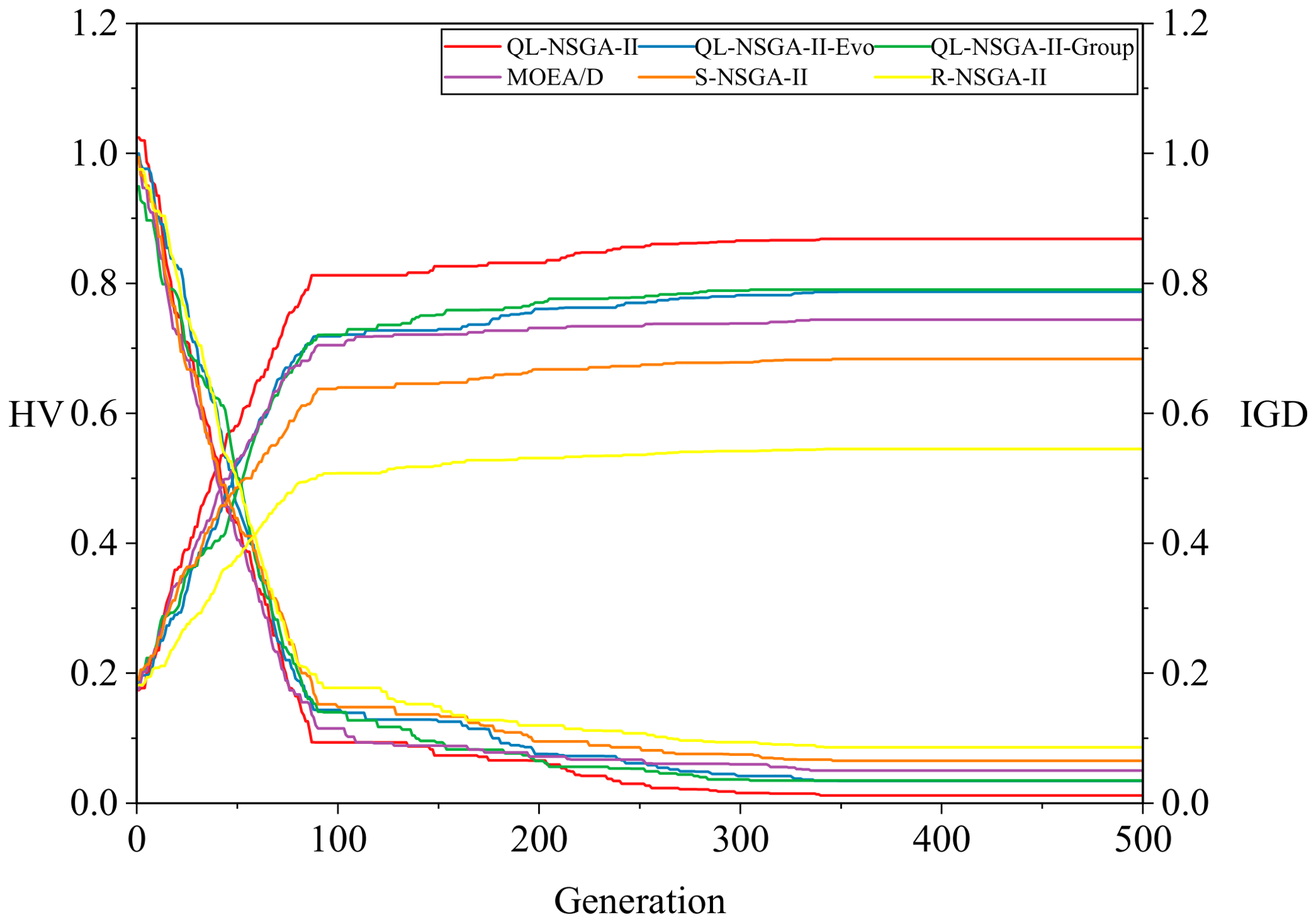
To further analyze the dynamic behavior of the algorithms during the evolutionary process, we extract the convergence trajectories of HV and IGD metrics over 500 generations, as well as the final Pareto fronts. It should be noted that for the proposed QL-NSGA-II and its Q-table-based variants, the convergence trajectory data are obtained from a single independent test run guided by the fully converged Q-tables after the agent has completed all training episodes.

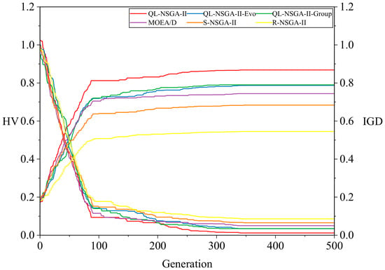
From the dynamic convergence curves of HV and IGD in Figure 8 on the P87 instance, it can be observed that all six algorithms undergo a rapid improvement phase in the first 100 generations, characterized by a notable rise in HV and a considerable decline in IGD. As evolution progresses into the middle and later stages, the convergence trajectories of QL-NSGA-II-Evo and several traditional comparison algorithms gradually flatten, indicating premature stagnation. In contrast, the proposed QL-NSGA-II algorithm, with its dynamic adjustment of the dual-Q-table exploration strategy, maintains relatively sustained fine-tuning capability even in the later evolutionary stages. Its HV curve eventually converges to a relatively higher level among all comparison algorithms, while its IGD curve smoothly decreases to a relatively lower range. This dynamic process intuitively indicates that introducing the dual-action-space mechanism in QL-NSGA-II helps preserve search vitality and robustness in frontier approximation for the population within the complex PC component grouping and scheduling space.

Figure 8. Convergence performance of HV and IGD for all algorithms on P87.

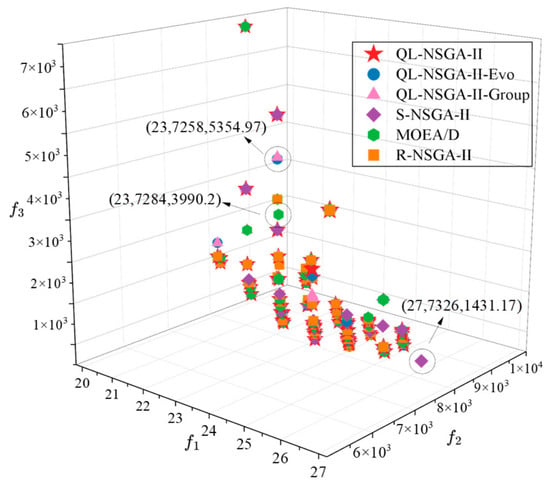
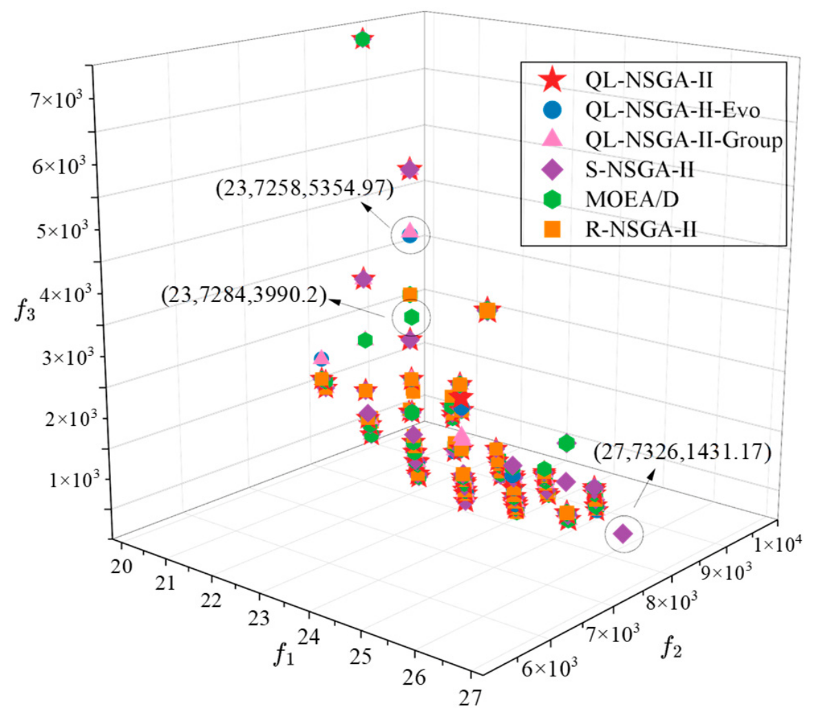
To further analyze the dynamic behavior of the algorithms during the evolutionary process, the final Pareto fronts obtained by each algorithm, as shown in Figure 9. The non-dominated solution set generated by the proposed QL-NSGA-II algorithm (marked with red stars) exhibits a generally favorable convergence trend, with its scattered points enveloping most of the solutions obtained by the other algorithms in the objective space. Additionally, some optimal solutions from the compared algorithms are dominated by those from QL-NSGA-II. For example, the solution (23, 7258, 5354.97) obtained by QL-NSGA-II-Evo and QL-NSGA-II-Group is dominated by (23, 7257, 3632.37) from QL-NSGA-II; the solution (23, 7284, 3990.2) from MOEA/D is dominated by (23, 7278, 2981.3); and the solution (27, 7326, 1431.17) from S-NSGA-II is dominated by (25, 7325, 1430.83), among other examples.

Figure 9. Comparison of Pareto solution distributions among algorithms.

5.4.3. Grouping and Scheduling Scheme for PC Components

To further analyze QL-NSGA-II’s decision-making mechanism in handling the conflict between spatial grouping and temporal sequencing of PC components, Table 4 lists the component grouping schemes on pallets when the three optimization objectives reach their respective minima. When the algorithm prioritizes minimizing the number of pallets, physical space utilization takes higher priority, and all 87 PC components are arranged relatively compactly across only 20 pallets. To make full use of the effective pallet area, the algorithm frequently employs a mixed arrangement of multiple component types and orthogonal rotation operations within a single pallet. In contrast, when the algorithm focuses on reducing the makespan or lowering the total penalty cost, the constraint on grouping density is moderately relaxed, and the total number of pallets used increases to 26 and 25, respectively.

Table 4. Grouping schemes for PC component production on P87.

Pallet	PC Component/Group Layout Direction
	Minimum f1	Minimum f2	Minimum f3
1#	11/0–12/0–13/0–13/1	10/0–1/0–13/1–21/0–21/0	11/0–16/0–21/0–15/0–12/0
2#	19/0–7/0–21/0–15/0–3/0–12/0	18/0–6/0–13/1	13/1–14/0–6/0–21/0
3#	4/0–2/1–1/0–15/0–21/0	6/0–5/1–15/0–2/1–15/1	16/0–3/1–13/0–3/1–15/1
4#	2/0–14/1–1/1–5/0	5/0–3/0–19/1–2/0–12/0	7/0–10/0–19/0–10/0
5#	20/0–10/0–10/0–3/0	9/0–14/0–10/1–8/0–3/0	2/0–1/0–4/0–2/0
6#	6/1–9/0–6/1–8/0	16/0–17/0–10/0–9/0–12/0	20/0–18/0–10/0
7#	10/1–19/0–5/1–6/0	7/0–19/0–8/0	6/1–17/0–6/0
8#	9/1–8/1–17/1–18/0	11/0–11/0	8/0–9/0–19/1–5/0–8/0
9#	16/1–11/0–16/0	4/0–20/0	1/0–5/0–9/1
10#	13/0–3/1–4/0–16/1–21/0	1/0–6/0–16/0	11/0–12/1
11#	2/0–11/0–5/0–15/1	21/1–16/1–5/1–15/0–13/0–12/0	2/0–19/1–13/0–10/0–12/0–21/0
12#	8/0–6/1–13/1–16/0–8/1	4/1–2/0–13/1–2/0	11/0–6/1–1/1
13#	17/1–2/0–6/1–5/0	9/1–14/0–5/0–10/0–3/0	11/0–9/0–15/1–8/0
14#	7/0–1/0–15/0–10/0	20/0–1/0–8/0–15/0	5/1–18/0–16/0–3/1–15/0
15#	19/0–11/0–6/1–12/0	19/1–1/1–8/1–3/0–12/0	17/0–9/1–5/0–12/1–10/0
16#	20/0–1/1–12/0–10/1–3/0	7/0–10/0–9/0	6/0–3/1–16/0–8/1
17#	14/1–18/1–9/1–9/1	11/0–6/0	6/1–2/0–4/1
18#	14/0–13/1–6/1–13/1	6/0–6/0	13/0–1/0–14/0
19#	2/0–5/0–6/1–5/0–2/0	11/0–16/0	20/0
20#	2/0–13/1–13/1–2/1–5/0	18/0–17/1	7/0
21#	×	5/1–13/0–13/0	6/1–13/0–2/0
22#	×	5/0–14/0	14/0–13/0–5/1
23#	×	2/0–6/0–2/0	2/1–6/1–5/1
24#	×	6/0	13/0–13/0–5/0
25#	×	13/0–13/0–5/1	2/0–2/0
26#	×	2/1–2/0	×

Note: The symbols ×, indicates that the pallet is not utilized.

This loosening of spatial distribution indicates that, in exchange for smoother process flow rhythm and more flexible delivery control, the agent tends to dilute the processing load of a single transfer by increasing pallet batches, thereby reducing queuing backlog at critical stages such as steam curing. For example, in Table 4, the grouping scheme that minimizes the penalty cost activates a total of 25 pallets, with an average of 3.48 components per pallet, and the total penalty cost is 647.87. In contrast, the scheme that minimizes the number of activated pallets uses a total of 20 pallets, with an average of 4.35 components per pallet, and incurs a total penalty cost of 7748.47.

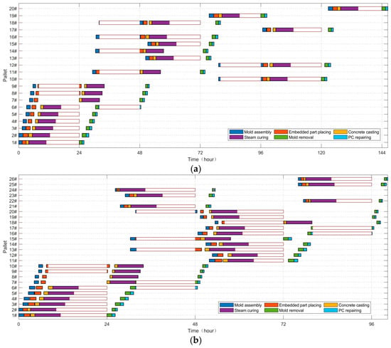
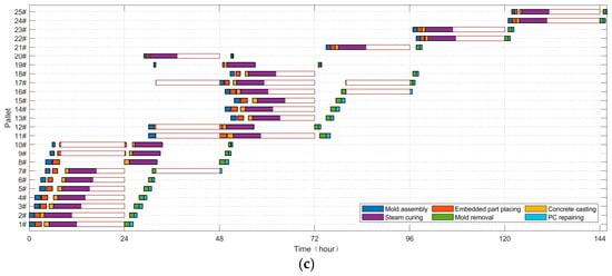
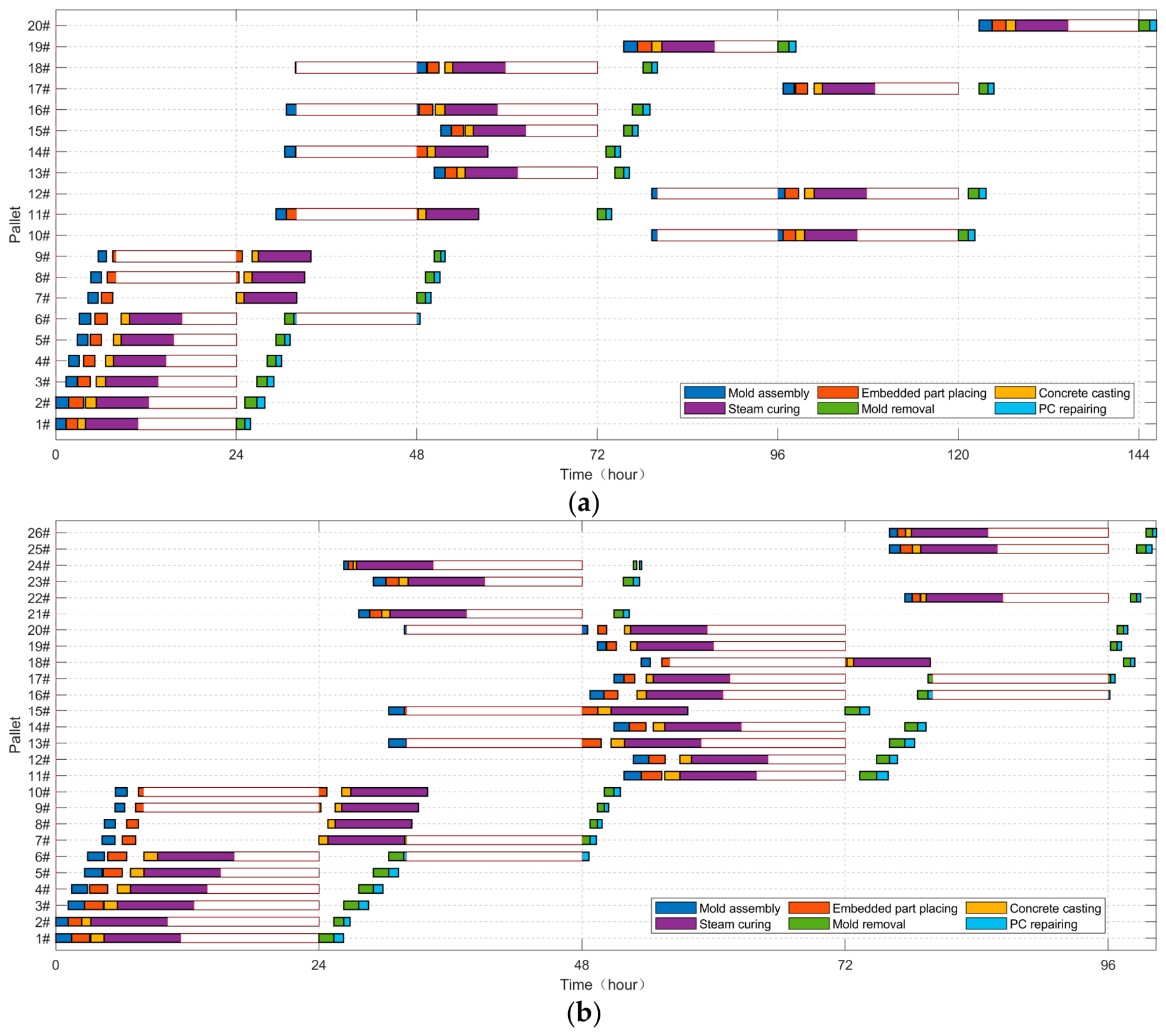
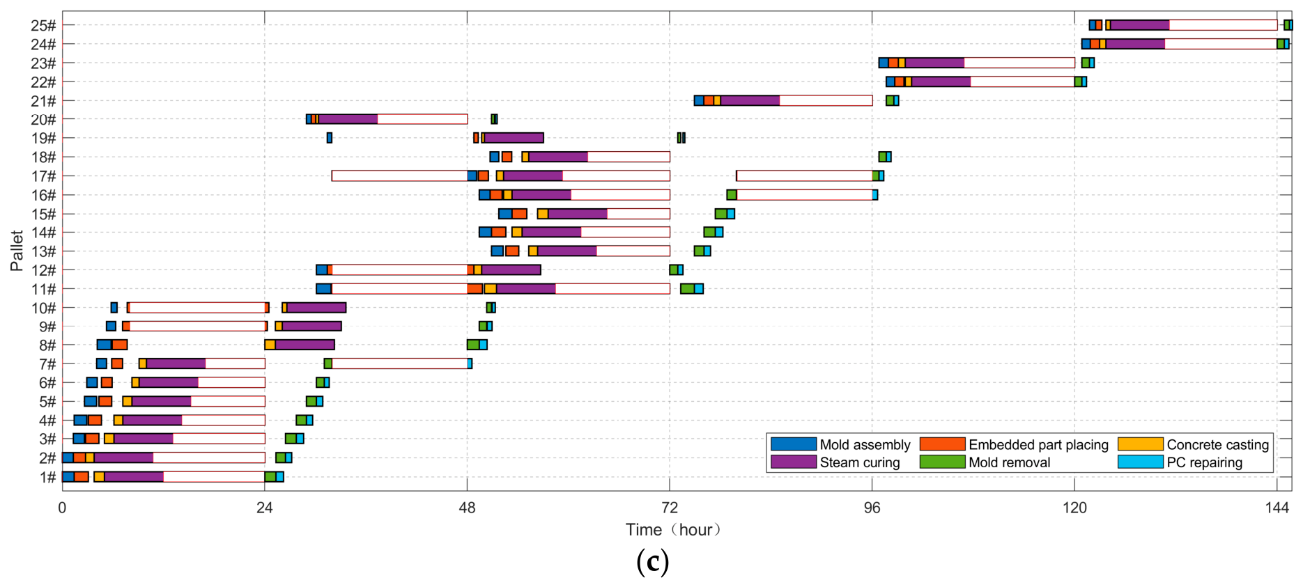
For the three PC component grouping schemes that reflect different optimization preferences, Figure 10 presents the workshop scheduling Gantt charts when the three objectives reach their minimum values, intuitively reflecting the algorithm’s differentiated decision-making characteristics in time resource allocation. When the algorithm is primarily oriented toward minimizing the number of pallets, the Gantt chart in Figure 10a shows a considerable number of long white blank areas between operations, indicating waiting time. In particular, before entering the resource-constrained steam-curing stage, the pallets experience a significant backlog, which extends the makespan of the entire order batch to around 144 h.

Figure 10. Scheduling schemes for PC component production on P87. (a) Scheduling scheme for P87 with minimum f₁. (b) Scheduling scheme for P87 with minimum f₂. (c) Scheduling scheme for P87 with minimum f₃.

In contrast, when the optimization objective shifts to minimizing the makespan, as shown in Figure 10b, the connections between operations become compact, the idle waiting time between operations is considerably reduced, and the production cycle of the entire batch is effectively controlled within 96 h, presenting a relatively efficient and smooth continuous manufacturing rhythm.

In addition, when the model focuses on minimizing the penalty cost, as shown in Figure 10c, the system uses a total of 25 pallets. Although its time span also extends to about 144 h, the distribution trajectory of its scheduling time exhibits a characteristic stepped pattern. The start times of the pallets are intentionally dispersed. For example, some tasks are strategically delayed until 48 or 120 h before initiation. This non-centralized scheduling layout is an adaptive scheduling decision made by the agent to anchor the differentiated delivery time windows of various components in the order. By reasonably inserting idle buffer periods between operations, QL-NSGA-II achieves a favorable balance between the inventory holding cost due to early completion and the tardiness penalty due to delayed delivery.

6. Conclusions

This study addresses the highly coupled problem of component grouping on pallets and production scheduling in precast component manufacturing by proposing a hybrid multi-objective optimization framework that integrates Q-learning with the non-dominated sorting genetic algorithm, termed QL-NSGA-II. The model aims to collaboratively minimize the number of pallets used, the makespan, and the penalty cost. The algorithm constructs a dual Q-table Markov decision architecture, in which a Q-learning agent adaptively coordinates PC component grouping and scheduling strategies based on hypervolume feedback from the evolutionary state. Through single-objective extreme tests on multiple benchmark instances from the literature, the results show that the proposed algorithm not only achieves the accuracy of benchmark solutions but also reduces the makespan and penalty cost by 34.77% and 60.24%, respectively, under certain complex configurations. In a multi-objective test on a real engineering order containing 87 components, based on 20 independent runs and the Wilcoxon rank-sum test at a significance level of 0.05, the complete QL-NSGA-II exhibits statistically significant advantages in both hypervolume and inverted generational distance metrics, effectively overcoming the drawback of being prone to local stagnation that affects the ablation variants and six comparison algorithms such as the traditional S-NSGA-II. Meanwhile, by analyzing grouping and scheduling schemes on the Pareto front, the model can provide visualized PC component production schedules for the workshop. This confirms that the proposed algorithm has good practical application potential in balancing pallet resource consumption and flow cycle.

Although the model and algorithm have achieved certain results in static scheduling scenarios, the existing framework has not yet fully accounted for dynamic disturbances in the workshop, such as equipment failures and urgent order insertions. At the same time, traditional discrete Q-tables are easily constrained by the dimension of the state space when dealing with larger-scale production scheduling. Future research will extend this joint scheduling model to uncertain manufacturing environments and explore the introduction of deep reinforcement learning mechanisms capable of handling high-dimensional continuous states, thereby breaking through the high-dimensional state space bottleneck encountered in large-scale production scheduling and further enhancing the algorithm’s generalization and adaptive capabilities in complex industrial scenarios.

References

- Zheng, R.; Li, Z.; Li, L.; Ma, S.; Li, X. Group Technology Empowering Optimization of Mixed-Flow Precast Production in off-Site Construction. Environ. Sci. Pollut. Res. 2024, 31, 11781–11800. [Google Scholar] [CrossRef] [Scilit] [PubMed]
- Chen, G.; Huang, J.; Wang, J.; Wei, J.; Shou, W.; Cao, Z.; Pan, W.; Zhou, J. Optimal Procurement Strategy for Off-Site Prefabricated Components Considering Construction Schedule and Cost. Autom. Constr. 2023, 147, 104726. [Google Scholar] [CrossRef] [Scilit]
- Arashpour, M.; Wakefield, R.; Abbasi, B.; Lee, E.W.M.; Minas, J. Off-Site Construction Optimization: Sequencing Multiple Job Classes with Time Constraints. Autom. Constr. 2016, 71, 262–270. [Google Scholar] [CrossRef] [Scilit]
- He, W.; Li, W.; Meng, X. Scheduling Optimization of Prefabricated Buildings under Resource Constraints. KSCE J. Civ. Eng. 2021, 25, 4507–4519. [Google Scholar] [CrossRef] [Scilit]
- Xiong, F.; Chen, X.; Liu, H.; Xiong, M.; Wu, M. The Flow Shop Batch Scheduling Problem in a Prefabricated Component Manufacturing System with Two-Dimensional Bin Packing Constraints. Int. J. Prod. Res. 2025, 63, 7196–7237. [Google Scholar] [CrossRef] [Scilit]
- Wang, Z.; Xu, H. Scheduling Redundancy Optimization for Precast Production to Enhance Disruption Management in Prefabricated Construction. Comput. Ind. Eng. 2024, 192, 110251. [Google Scholar] [CrossRef] [Scilit]
- Liu, F.; Deng, X.; Peng, W.; Li, J.; Li, H.; Li, C. Scheduling Optimization for the Production of Prefabricated Components Considering Batch Production on Mold Tables. Eng. Optim. 2025, 57, 2960–2983. [Google Scholar] [CrossRef] [Scilit]
- Wang, D.; Liu, G.; Li, K.; Wang, T.; Shrestha, A.; Martek, I.; Tao, X. Layout Optimization Model for the Production Planning of Precast Concrete Building Components. Sustainability 2018, 10, 1807. [Google Scholar] [CrossRef] [Scilit]
- Kong, L.; Li, H.; Luo, H.; Lieyun, D.; Luo, X.; Skitmore, M. Optimal Single-Machine Batch Scheduling for the Manufacture, Transportation and JIT Assembly of Precast Construction with Changeover Costs within Due Dates. Autom. Constr. 2017, 81, 34–43. [Google Scholar] [CrossRef] [Scilit]
- Liang, J.; Liu, Y.; Sun, X.; Xu, W.; Du, B. Multi-Objective Optimization of Production Sequence and Layout of Precast Concrete Components on the Mold Table Under Limited Mold Quantity. Buildings 2026, 16, 951. [Google Scholar] [CrossRef] [Scilit]
- Chan, W.T.; Hu, H. Production Scheduling for Precast Plants Using a Flow Shop Sequencing Model. J. Comput. Civ. Eng. 2002, 16, 165–174. [Google Scholar] [CrossRef] [Scilit]
- Wang, Z.; Hu, H.; Gong, J.; Ma, X. Synchronizing Production Scheduling with Resources Allocation for Precast Components in a Multi-Agent System Environment. J. Manuf. Syst. 2018, 49, 131–142. [Google Scholar] [CrossRef] [Scilit]
- Wang, Z.; Hu, H. Dynamic Response to Demand Variability for Precast Production Rescheduling with Multiple Lines. Int. J. Prod. Res. 2018, 56, 5386–5401. [Google Scholar] [CrossRef] [Scilit]
- Yuan, Z.; Li, Z.; Lei, Z.; Yang, Y.; Zhang, W.; Lin, W.; Cao, L. Enhancing the Production Performance of Prefabricated Buildings through the Integrated Optimization of Precast Component Layout and Worker Allocation. J. Constr. Eng. Manag. 2025, 151, 1–14. [Google Scholar] [CrossRef] [Scilit]
- Dawood, N.N. Scheduling in the Precast Concrete Industry Using the Simulation Modelling Approach. Build. Environ. 1995, 30, 197–207. [Google Scholar] [CrossRef] [Scilit]
- Chan, W.T.; Hu, H. Precast Production Scheduling with Genetic Algorithms. Proc. IEEE Conf. Evol. Comput. ICEC 2000, 2, 1087–1094. [Google Scholar] [CrossRef] [Scilit]
- Chan, W.T.; Hu, H. Constraint Programming Approach to Precast Production Scheduling. J. Constr. Eng. Manag. 2002, 128, 513–521. [Google Scholar] [CrossRef] [Scilit]
- Leu, S.S.; Hwang, S.T. GA-Based Resource-Constrained Flow-Shop Scheduling Model for Mixed Precast Production. Autom. Constr. 2002, 11, 439–452. [Google Scholar] [CrossRef] [Scilit]
- Benjaoran, V.; Dawood, N.; Hobbs, B. Flowshop Scheduling Model for Bespoke Precast Concrete Production Planning. Constr. Manag. Econ. 2005, 23, 93–105. [Google Scholar] [CrossRef] [Scilit]
- Yang, Z.; Ma, Z.; Wu, S. Optimized Flowshop Scheduling of Multiple Production Lines for Precast Production. Autom. Constr. 2016, 72, 321–329. [Google Scholar] [CrossRef] [Scilit]
- Ma, Z.; Yang, Z.; Liu, S.; Wu, S. Optimized Rescheduling of Multiple Production Lines for Flowshop Production of Reinforced Precast Concrete Components. Autom. Constr. 2018, 95, 86–97. [Google Scholar] [CrossRef] [Scilit]
- Liu, W.; Tao, X.; Mao, C.; He, W. Scheduling Optimization for Production of Prefabricated Components with Parallel Work of Serial Machines. Autom. Constr. 2023, 148, 104770. [Google Scholar] [CrossRef] [Scilit]
- Dan, Y.; Liu, G.; Fu, Y. Optimized Flowshop Scheduling for Precast Production Considering Process Connection and Blocking. Autom. Constr. 2021, 125, 103575. [Google Scholar] [CrossRef] [Scilit]
- Ko, C.H.; Wang, S.F. Precast Production Scheduling Using Multi-Objective Genetic Algorithms. Expert Syst. Appl. 2011, 38, 8293–8302. [Google Scholar] [CrossRef] [Scilit]
- Du, J.; Dong, P.; Sugumaran, V. Dynamic Production Scheduling for Prefabricated Components Considering the Demand Fluctuation. Intell. Autom. Soft Comput. 2020, 26, 715–723. [Google Scholar] [CrossRef] [Scilit]
- Kim, T.; Kim, Y.W.; Cho, H. Dynamic Production Scheduling Model under Due Date Uncertainty in Precast Concrete Construction. J. Clean. Prod. 2020, 257, 120527. [Google Scholar] [CrossRef] [Scilit]
- Wang, Z.; Liu, Y.; Hu, H.; Dai, L. Hybrid Rescheduling Optimization Model under Disruptions in Precast Production Considering Real-World Environment. J. Constr. Eng. Manag. 2021, 147, 1–16. [Google Scholar] [CrossRef] [Scilit]
- Zhang, R.; Feng, X.; Mou, Z.; Zhang, Y. Green Optimization for Precast Production Rescheduling Based on Disruption Management. J. Clean. Prod. 2023, 420, 138406. [Google Scholar] [CrossRef] [Scilit]
- Wang, L.; Zhao, Y.; Yin, X. Precast Production Scheduling in Off-Site Construction: Mainstream Contents and Optimization Perspective. J. Clean. Prod. 2023, 405, 137054. [Google Scholar] [CrossRef] [Scilit]
- Xiong, F.; Chen, S.; Ma, Z.; Li, L. Approximate Model and Algorithms for Precast Supply Chain Scheduling Problem with Time-Dependent Transportation Times. Int. J. Prod. Res. 2023, 61, 2057–2085. [Google Scholar] [CrossRef] [Scilit]
- Xiong, F.; Chu, M.; Li, Z.; Du, Y.; Wang, L. Just-in-Time Scheduling for a Distributed Concrete Precast Flow Shop System. Comput. Oper. Res. 2021, 129, 105204. [Google Scholar] [CrossRef] [Scilit]
- Chang, C.; Han, M. Production Scheduling Optimization of Prefabricated Building Components Based on DDE Algorithm. Math. Probl. Eng. 2021, 2021, 6672753. [Google Scholar] [CrossRef] [Scilit]
- Jiang, W.; Wu, L. Flow Shop Optimization of Hybrid Make-to-Order and Make-to-Stock in Precast Concrete Component Production. J. Clean. Prod. 2021, 297, 126708. [Google Scholar] [CrossRef] [Scilit]
- Arashpour, M.; Bai, Y.; Aranda-mena, G.; Bab-Hadiashar, A.; Hosseini, R.; Kalutara, P. Optimizing Decisions in Advanced Manufacturing of Prefabricated Products: Theorizing Supply Chain Configurations in off-Site Construction. Autom. Constr. 2017, 84, 146–153. [Google Scholar] [CrossRef] [Scilit]
- Yuan, Z.; Qiao, Y.; Guo, Y.; Wang, Y.; Chen, C.; Wang, W. Research on Lean Planning and Optimization for Precast Component Production Based on Discrete Event Simulation. Adv. Civ. Eng. 2020, 2020, 8814914. [Google Scholar] [CrossRef] [Scilit]
- Larsson, J.; Lu, W.; Krantz, J.; Olofsson, T. Discrete Event Simulation Analysis of Product and Process Platforms: A Bridge Construction Case Study. J. Constr. Eng. Manag. 2016, 142, 1–12. [Google Scholar] [CrossRef] [Scilit]
- Li, Y.; Wu, J.; Hao, Y.; Gao, Y.; Chai, R.; Chai, S.; Zhang, B. Automation in Construction Process Scheduling for Prefabricated Construction Based on Multi-Objective Optimization Algorithm. Autom. Constr. 2024, 168, 105809. [Google Scholar] [CrossRef] [Scilit]
- Zu, L.; Liao, W. Reinforcement Learning–Based Multiobjective and Multiconstraint Production Scheduling for Precast Concrete. J. Constr. Eng. Manag. 2025, 151, 8. [Google Scholar] [CrossRef] [Scilit]
- Kim, T.; Kim, Y.W.; Lee, D.; Kim, M. Reinforcement Learning Approach to Scheduling of Precast Concrete Production. J. Clean. Prod. 2022, 336, 130419. [Google Scholar] [CrossRef] [Scilit]
- Yang, R.; Xu, S.; Li, H.; Zhu, H.; Zhao, H.; Wang, X. Action-Oriented Deep Reinforcement Learning Method for Precast Concrete Component Production Scheduling. Buildings 2025, 15, 697. [Google Scholar] [CrossRef] [Scilit]
- Zheng, R.; Li, Z.; Li, L.; Dou, Y.; Yuan, M.; Yin, X. Proposing a Lean-Optimized Scheduling Model of Mixed-Flow Prefabricated Component Production in Off-Site Construction. J. Constr. Eng. Manag. 2024, 150, 1–15. [Google Scholar] [CrossRef] [Scilit]
- Xiang, Y.; Duan, P.; Wang, J.; Jiang, G.; Hu, Z.; Xiao, Q.; Zeng, X. Optimization of Steam Curing Process for Chinese Western and Northeast Regions’ High-Speed Railway Concrete Prefabricated Components. Struct. Concr. 2025, 26, 1338–1352. [Google Scholar] [CrossRef] [Scilit]
- Leu, S.S.; Hwang, S.T. A GA-Based Model for Maximizing Precast Plant Production under Resource Constraints. Eng. Optim. 2001, 33, 619–642. [Google Scholar] [CrossRef] [Scilit]
- Qin, S.; Zhang, X.; Wang, J.; Guo, X.; Qi, L.; Cao, J.; Liu, Y. An Improved Q-Learning Algorithm for Optimizing Sustainable Remanufacturing Systems. Sustainability 2024, 16, 4180. [Google Scholar] [CrossRef] [Scilit]
- Yang, W.; Li, Z.; Zheng, C.; Li, T.; Zhang, Z.; Zhang, L. A Q-Learning-Oriented Multi-Objective Teaching-Learning-Based Optimization Algorithm for Balancing U-Shaped Disassembly Lines. Appl. Soft Comput. 2025, 177, 113273. [Google Scholar] [CrossRef] [Scilit]
- Ko, C.H.; Wang, S.F. GA-Based Decision Support Systems for Precast Production Planning. Autom. Constr. 2010, 19, 907–916. [Google Scholar] [CrossRef] [Scilit]
Disclaimer/Publisher’s Note: The statements, opinions and data contained in all publications are solely those of the individual author(s) and contributor(s) and not of MDPI and/or the editor(s). MDPI and/or the editor(s) disclaim responsibility for any injury to people or property resulting from any ideas, methods, instructions or products referred to in the content. |
© 2026 by the authors. Licensee MDPI, Basel, Switzerland. This article is an open access article distributed under the terms and conditions of the Creative Commons Attribution (CC BY) license.