


Abstract
Opening hours are frequently reused as occupancy schedules in building-energy assessment, although access availability and occupation describe different temporal conditions. This paper quantifies this difference and relates both to metered electricity consumption in the teaching stock of the Universitat Politècnica de Catalunya · BarcelonaTech (UPC). Published access schedules for 2025 were compiled for its eighteen teaching centers, and hourly electricity from ten verified smart meters was classified into three mutually exclusive states: (a) teaching hours, (b) open hours outside teaching hours, and (c) closed hours. At the university level, teaching hours were approximated by each center’s general teaching-hours window. Across the eighteen centers, buildings were open for about 30% to 52% of the year’s hours and closed for the remaining hours (48.3–70.5%). The share of recorded electrical consumption, however, varies in each of the categories: (a) teaching hours carried 28.5–40.4% of the recorded annual consumption in 18.2–21.7% of the time, (b) open hours outside teaching carried 19.0–36.4% in 12.5–31.7% of the year, and (c) closed hours (although being the longest state) carried 23.2–51.9%. The Barcelona School of Architecture (ETSAB) was used as a detailed case study where teaching hours were also resolved room-by-room. At least one classroom was timetabled during 21.5% of the year’s hours, the mean classroom was timetabled for 7.1% of the year (about a seventh of the building’s accessible time) and the open hours without timetabled teaching covered 26.7% of the calendar hours and 31.0% of the recorded consumption. Across the full week, whole-building consumption followed the general daily teaching-hours window (r = 0.92) more closely than the classroom timetable fraction (r = 0.77). Pooled across the ten classified meters on recorded hours, taking an “open hour without teaching” as the reference intensity (1.00), closed hours ran at 0.57 and teaching hours at 1.20.
1. Introduction
Occupancy schedules are standard inputs to building-energy assessment and simulation. They determine when internal gains, ventilation requirements and occupancy-dependent system loads are applied, and normative calculation frameworks prescribe them explicitly. EN 16798-1:2019 and, in Spain, the Código Técnico de la Edificación [1] offer normalized user profiles to be used in standard energy calculations. Simulation outcomes are sensitive to that assumption: varying the representation of users changes predicted demand enough to alter design decisions [2], the timing and variability of occupancy governs heating and cooling loads [3], and control strategies that act on occupancy information rather than on a fixed schedule change predicted consumption appreciably [4]. The inadequate treatment of occupancy is accordingly one of the recognized contributors to the discrepancy between predicted and observed energy use [5,6,7,8]. Yet the source and meaning of the profile applied are not always explicit.
Occupant-behavior research tries to fill this gap by producing stochastic models of presence and of occupant interaction with building systems [9,10] together with field implementations of occupant-centric control [11]. However, urban building-energy modeling studies report that stereotyped schedules per use type remain the usual representation of occupancy [12]. Whether a stereotyped schedule is adequate depends on the purpose of the model: fit-for-purpose strategies match the occupancy description to the simulation objective [13]. Yet a building’s opening schedule defines when it is accessible, not when its rooms are actually in use, how intensively they are used, or whether people are present.
Educational buildings are a case in which the distinction between access and use is unusually large and unusually well documented. School and academic calendars commonly close during weekends, public holidays and long non-academic periods. Within the remaining opening window, timetables assign each classroom for only part of the day, pointing to periods with expected highest occupancy in the building. Both schedules are frequently openly published on schools’ websites.
Research on educational spaces has a strong background on topics such as indoor environmental quality and thermal comfort in relationship with occupancy in classrooms. A post-occupancy assessment of three higher-education buildings of more than 50,000 m2 in the Paris region identifies occupancy as the main driver of electricity use, with the occupancy profiles taken from typical office hours and absence rates rather than from institutional records [14]. Reported energy-use intensities across 80 higher-education buildings in Australia vary in a proportion of roughly 1:2 between disciplines and activities [15]. One year of sub-metered data from an educational building in Melbourne reports electricity and gas consumption is 2.4 and 3.1 times the design prediction, with 48% of annual energy consumed during non-working hours and the mechanical system and plug loads following the weekday operating schedule during holiday closures [16]. On a Spanish university campus, continuous temperature and CO2 monitoring were used as parameters for a demand-controlled HVAC in classrooms of fluctuating occupancy, cutting HVAC consumption by a reported 40–70% [17], indicating the importance of occupancy in energy systems.
Three studies were found to relate an occupancy record directly to metered energy. In one university building, published room timetables for six teaching rooms were compared with electricity demand, and it was determined that they are not strongly correlated [18]. On the MIT university campus, WiFi connection counts tracked metered electricity moderately well but HVAC operation only weakly [19]. In offices, measurements from 629 motion sensors deviated from the diversity factors published in energy-code guidance by up to 46% [20]. In each of these three, the occupancy reference used is a measured proxy, an assumed profile, or a timetable covering part of a year, and a building’s own access schedule is not treated as distinct from occupancy or teaching. More recently, higher-education studies have shown that replacing generic schedules with class-reservation schedules alters simulated ventilation, occupancy density and energy demand [21], that campus-level demand models improve when building-specific occupancy profiles replace uniform schedules [22,23], and that university building occupancy follows term, examination, weekend and holiday drivers rather than opening hours [24]. Dynamic simulation of a university teaching building has likewise shown that substituting room-resolved timetables for generic schedules changes simulated electricity demand [25]. Yet these studies focus on occupancy records or simulated demand. How published opening schedules, classroom timetables and metered electricity relate across a multi-campus building stock remains an open question.
This paper analyzes published access schedules for the eighteen teaching centers of the Universitat Politècnica de Catalunya · BarcelonaTech (UPC) together with 2025 hourly electricity from ten verified smart meters covering twelve centers (12/18) on eight out of nine (8/9) campuses. A nested case study at the Barcelona School of Architecture (ETSAB), one of the metered centers, adds the timetables of its 45 classrooms. Specifically, this paper asks: (RQ1) What fraction of the year is covered by an educational building’s opening schedule, and what fraction by its classrooms’ teaching schedules? (RQ2) How is electricity consumption distributed across hours in which (a) teaching is scheduled, (b) the building is open but no teaching is scheduled, and (c) the building is closed? (RQ3) How much does a building-level approximation of teaching time distort that distribution relative to room-resolved timetables?
2. Materials and Methods
This study combines opening schedules with metered hourly electricity at two levels of resolution: at the university level and at the building level.
At the university level, access schedules for the eighteen teaching centers of the Universitat Politècnica de Catalunya · BarcelonaTech (UPC) are compared with hourly electricity consumption. Electricity consumption was exported from Sirena, the centralized monitoring platform that records data from UPC’s buildings and classrooms on all campuses.
At the building level, one of those centers, the Barcelona School of Architecture (ETSAB), is examined in detail: its teaching schedule is resolved from the individual timetables of its 45 classrooms instead of using a generic teaching schedule. Its electricity consumption is classified into the same three mutually exclusive states. Because ETSAB is classified at the university level and as a detailed case study, it is used as a reference comparison in the discussion.
All the data retrieved for this analysis was limited to the calendar year 2025, from 1st January to 31st December.
2.1. Concepts Used in This Analysis
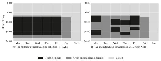
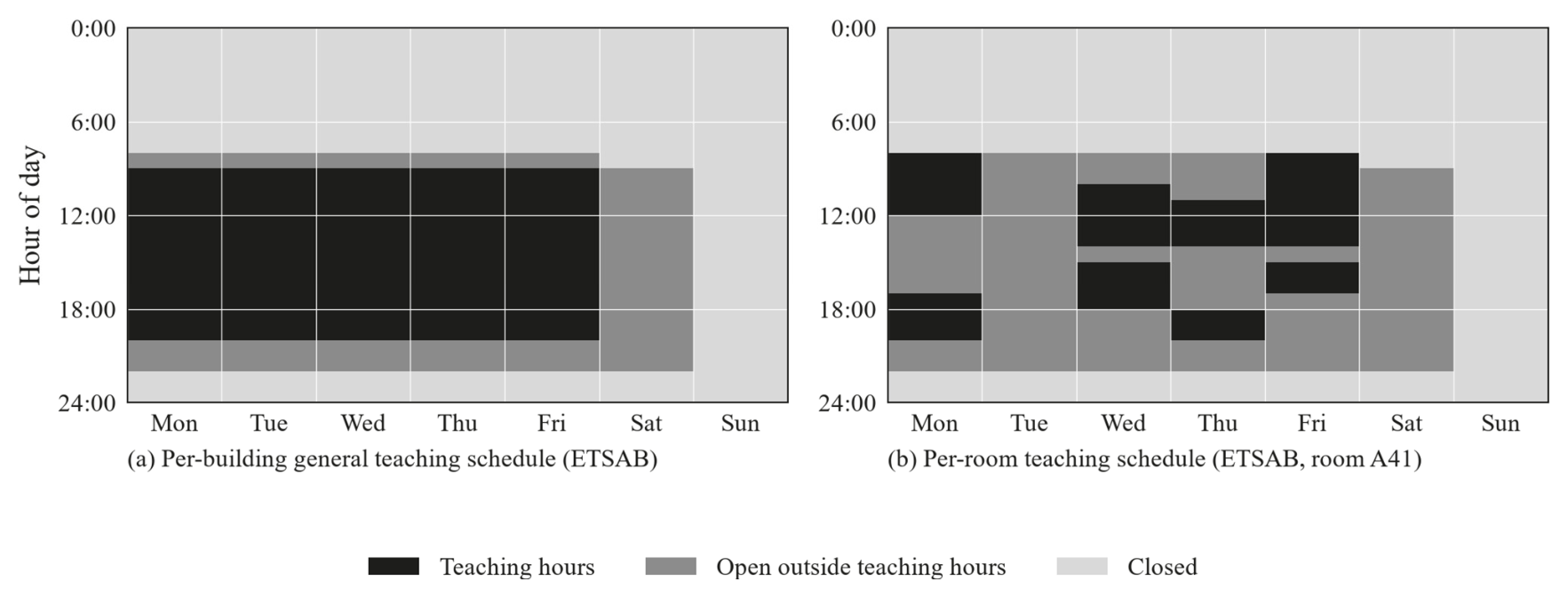
This paper uses some terms that are defined here to clarify in advance the scope of each of them. Figure 1 illustrates the three schedule-defined states over one reference (generic) scheduled week at ETSAB (a) and for classroom A-41 (b).
Figure 1.
Schedule-defined states over the ETSAB reference week (20–26 October 2025): (a) the general teaching-hours window at the building level labels every weekday hour from 8:30 to 20:00 as teaching, whereas (b) the room-resolved teaching schedule of a single classroom (A41) is timetabled only in a subset of those hours.
- •
- The opening schedule is the access schedule and answers “when the building could be entered”. The energy intensity use varies during the opening hours.
- •
- The teaching schedule is embedded in the opening schedule but just considers the hours “when classrooms are planned to host lessons”. During this period, higher-intensity use is expected in educational buildings.
- •
- The closing schedule is the opposite of the opening schedule and indicates “when the building is planned to be closed to public”. Even with no occupation, some energy-consuming systems remain active, such as IT servers, lifts, and emergency systems.
2.2. The Case Study: University Building Stock
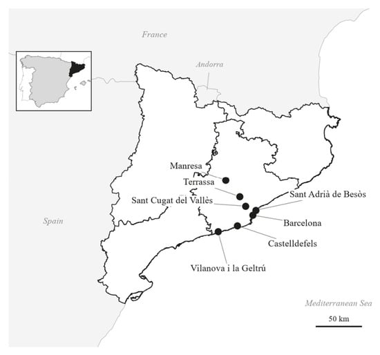
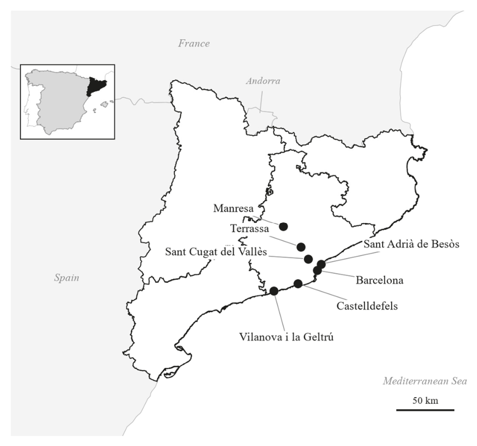
This study comprises the eighteen teaching centers of the Universitat Politècnica de Catalunya · BarcelonaTech (UPC), distributed over nine campuses in seven municipalities in Catalonia, Spain: Barcelona, Sant Adria del Besòs, Castelldefels, Vilanova i la Geltrú, Sant Cugat del Vallès, Terrassa and Manresa (Figure 2). The centers span architecture, building construction, civil, industrial, telecommunications, aerospace, agri-food, nautical, optics, multimedia engineering, mathematics and informatics studies. They share one academic calendar, but each center sets its own building access schedule, which is what makes the comparison between access and teaching possible within a single institution.
Figure 2.
Municipalities with campuses of the Universitat Politècnica de Catalunya · BarcelonaTech (UPC) (Catalonia, Spain).
2.3. Data Sources and Classification Method
Published access schedules were compiled for each center from its official building-hours or access-calendar page. Where no official information was clear, the center reception was contacted directly. For every center, the compiled schedule records the weekday access window, any weekend service, local festivities and documented closure periods. Appendix A lists the source, scope and consultation date for every center.
The academic calendar fixes the two 2025 term-time periods common to all centers, 10 February to 30 May and 8 September to 19 December, from which public holidays, local festivities and documented per-center closures are removed. Each center’s teaching-hours window was taken from its published timetable structure. The windows differ across centers and are reported with the results in Table 2, so the teaching-hours state is not defined identically for every meter.
Each center’s hourly electricity consumption was retrieved from Sirena. However, some centers did not report data, or reported partial data, resulting in eleven valid meters. Each meter represented exactly one center, except for two that aggregated the consumption for two centers (EETAC and EEABB in Castelldefels, and FME and CFIS in Campus Sud). Every meter’s dataset was reviewed to identify missing data: missing hours arise from the daylight-saving transition, the 28–29 April 2025 Iberian blackout and platform gaps; ETSAB, for example, returned 8552 of the 8760 h (97.6% completeness), and the ten retained meters all achieved 97.6–99.5% completeness. Two metered centers were excluded from the state classifications: EPSEVG, where on-site photovoltaic generation masks daytime grid demand, and ETSEIB, which lacks 27.1% of the year (1 January to 10 March and 15 April to 3 May and ends on 16 December), biasing winter and spring representations. Meter data coverage for 2025 is reported in Table 1.
Table 1.
The eighteen UPC teaching centers: campus and municipality, evidence for the published access schedule, annual opening coverage as a share of the 8760 h of the year, 2025 electricity-meter coverage, and inclusion in the classified analysis. The twelve centers (ten meters) above the line are included in the classified electricity analysis.
For each of the meters, every observed hour was assigned to exactly one of three mutually exclusive schedule-defined states: (a) teaching hours, if the building was open on a term-time weekday within the teaching-hours window in some classrooms; (b) open outside teaching hours, hours inside the opening schedule but outside the teaching-hours window, which includes the weekend study-room services; or (c) closed, outside the opening schedule.
Hourly electricity records are stamped at the start of the hour (00:00 to 23:00). Because an hourly meter reading is indivisible, the classification convention used in this study assigns each record by the schedule status at the start of the hour. For example, for an opening hour at 07:30, the record at 7–8 h is considered closed and the record at 8–9 h is considered open. To quantify the sensitivity of these boundaries, shares are also computed under an inclusive overlap rule in which any hour partially overlapping a window (such as 7–8 h for a 07:30 start) is included in that state (Appendix C).
To express the results in this study, we opt for the following rule:
- •
- Schedule shares are expressed over the 8760 h of the year, so the three states (a + b + c) sum to 100%, since a schedule exists for every hour by construction.
- •
- Metered electricity consumption, however, contains a small fraction of hours without a valid reading (0.5–2.4% of the year across the ten classified meters). Because unrecorded hours are not metered energy, energy shares (%kWh) are calculated as percentages of recorded annual electricity consumption so that the three states (a + b + c) sum to 100.0% of measured energy, while the share of invalid/unrecorded hours is reported separately outside the %kWh calculation as a time-coverage indicator.
In the data analysis, the authors used generative AI models SWE-2.0, OpenAI GPT-5.6-Sol and Anthropic Claude Fable 5.1 from Devin AI (Cognition) for code drafting. The authors have reviewed and edited the output and take full responsibility.
2.4. Detailed Case Study: Per-Classroom Schedules at the Barcelona School of Architecture (ETSAB)
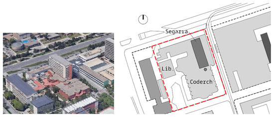
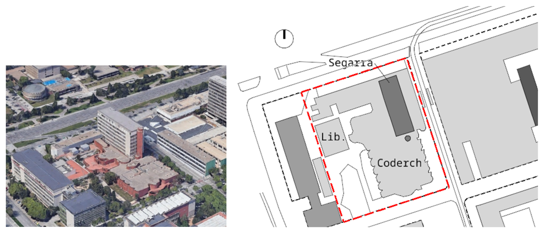
The ETSAB building stands at Avinguda Diagonal 649 in Barcelona (Campus Sud), and comprises two buildings with teaching classrooms, named Segarra and Coderch, plus a third detached building that hosts the library (Figure 3). The Segarra building is an eight-story building designed by the architect Josep Maria Segarra and built in 1961, containing the workshop and teaching classrooms together with most departments. The Coderch building extends the school over a ground floor and semi-basement, designed by the architect Josep Antoni Coderch in 1985, and contains teaching classrooms and the aula magna, among other services. The library occupies the third detached building, designed by Jaume Sanmarti Verdaguer in 2009. The gross floor area is 38,452 m2 according to the cadastral record [26], summing the Segarra (25,899 m2), Coderch (10,822 m2) and library (1731 m2).
Figure 3.
Aerial view (source: Google Earth) and site plan of the Barcelona School of Architecture (ETSAB–UPC), with indication of the two main buildings, Segarra and Coderch, and the library.
Because the analysis is based on metered electricity, it is relevant to know the main electrical loads of the complex. A single meter serves the whole complex, which besides classrooms contains academic-management and staff offices, study rooms, model-making and 3D-printing rooms, seminar and degree rooms, a copy shop, and a bar–cafeteria. Heating is non-electric; however, air conditioning serves the library and the Coderch building, while in the Segarra building it is limited to some academic-management and staff offices.
Classroom timetables were retrieved from the school’s public “occupancy per classroom” service for the 2025 term-time periods [27]. There are 47 classrooms in the complex: 26 in the Segarra building (A-labeled) and 21 in the Coderch building (C-labeled). Two Coderch rooms, C-B6 and C-S6, carry no timetable and were excluded as decommissioned under remodeling works, leaving 45 valid classrooms (26 Segarra and 19 Coderch) as part of the analysis. A 24 h by 7 d grid was built for each of the 45 classrooms from a regular mid-term teaching week published by the school service. Each cell records the scheduled fraction of the hour. While the general university calendar spans 38.5 academic weeks to encompass all academic activities, each school schedules regular classroom teaching during 14–15 weeks per semester (29.0 teaching weeks; 145 teaching weekdays) in the 2025 calendar (10 February to 30 May and 8 September to 19 December, excluding holidays and closures). Both the per-room annual teaching-schedule rate (weekly scheduled hours × 29.0/8760 h) and the hourly state classification project the reference week onto those 145 teaching weekdays. The dedicated examination weeks of January and June fall outside the regular teaching weeks and are not modeled separately, being classified as open hours without teaching.
Repeating the same analysis carried out at the university level, each observed meter hour was then assigned to one of three mutually exclusive states: (a) building open with at least one of the classrooms timetabled (using actual per-classroom schedules here, not generic teaching schedules per building); (b) building open with no classroom scheduled; or (c) building closed.
To examine how seasonal conditions affect the state intensities at the university level, observed hours were grouped by meteorological season (winter: December–February; spring: March–May; summer: June–August; autumn: September–November). Finally, to test whether the intra-day and intra-week shape of the classroom timetable is reflected in the whole-building electricity meter, the mean 168 h weekly consumption profile across the 2025 teaching weeks was compared with both the generic teaching-hours window and the scheduled classroom fraction.
3. Results
Results are reported at two resolutions. Section 3.1 describes the university-level analysis, where teaching time is derived from each center’s general teaching-hours window. Section 3.2 describes ETSAB results, where the teaching schedule is resolved in detail from the individual timetables of 45 classrooms. Section 3.3 evaluates the seasonal effect on the measured electricity consumption. Section 3.4 quantifies the difference between the two analysis levels using the ETSAB case study for comparisons since it is classified both ways. Section 3.5 tests whether the weekly profile shape of whole-building consumption follows the generic teaching window or the classroom timetables.
3.1. At the University Level
The university-level analysis is scoped to the eighteen buildings for the schedule analysis, and to the ten verified smart meters (twelve centers) for the electrical consumption analysis.
3.1.1. Opening Hours Versus Teaching Hours
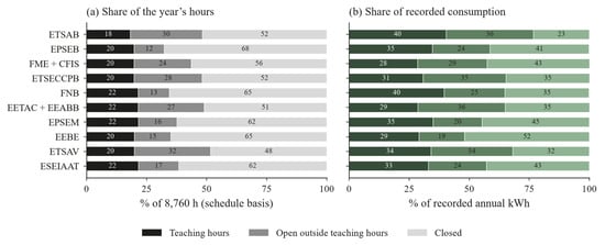
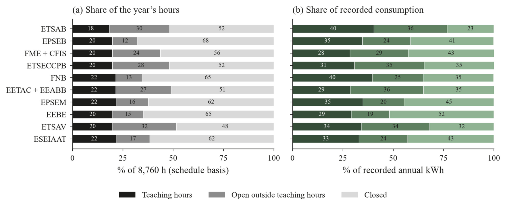
The opening schedules vary widely across the building stock. Among all eighteen centers, buildings were accessible during 29.5–51.7% of the year’s hours and closed during 48.3–70.5%. Across the ten analyzed meters, the generic teaching-hours window covers 18.2–21.7% of the year’s hours (Table 2, Figure 4), a spread that reflects the different window widths of the centers (11 to 13 h per day).
Figure 4.
Schedule-defined states across the ten classified meters: (a) share of the year’s 8760 calendar hours, in black, and (b) share of recorded annual electricity consumption, in green. Teaching hours indicate when teaching may occur anywhere in the building, not measured or timetabled use; aggregate and partial meter scopes are identified in the labels.
Table 2.
Access schedule and 2025 electricity consumption by schedule-defined state for the ten classified meters: generic teaching-hours window, number of teaching days, and the %h (share of 8760 calendar hours) and %kWh (share of recorded annual consumption, summing to 100.0%) for each state, and the percentage of invalid/unrecorded hours reported separately. * Teaching windows that start at 08:30 (marked with an asterisk) have 11 whole hours/day at ETSAB, and 12 at EEBE and ETSAV. We apply the start-of-hour rule in the electricity meter classification: an hourly reading is indivisible, so it is classified by the state at the start of the hour. See Appendix C, Table A3 for this boundary sensitivity analysis.
3.1.2. Electricity Consumption by Schedule-Defined State at the University Level
Table 2 summarizes each state with a pair of shares so that duration and energy appear side by side: %h is the share of the year’s 8760 h covered by each category (a + b + c = 100%), and %kWh is the share of each meter’s recorded annual electricity in each category (a + b + c = 100%), while the share of invalid or unrecorded hours (0.5–2.4% of the year) is reported in a separate column outside the %kWh calculation. Open hours are split into teaching hours (18.2–21.7% of the year’s hours carrying 28.5–40.4% of recorded consumption) and open hours with no teaching (12.5–31.7% carrying 19.0–36.4% of recorded consumption). Closed hours represent 48.3–67.6% of the year’s hours carrying 23.2–51.9% of recorded consumption (Table 2, Figure 4). Across the ten classified meters, recorded consumption amounted to 8.83 GWh in 2025: 2.73 GWh (31.0%) was recorded during teaching-hours windows, 2.40 GWh (27.2%) in open hours outside teaching, and the remaining 3.7 GWh (41.8%) in closed hours.
The three states differ in duration as well as in energy intensity use. Normalized to the mean hourly consumption of an open hour without teaching (b), teaching hours (a) ran at a proportion of 0.9–1.8 across meters, while closed hours (c) ran between 0.27 and 0.63 (Table 3). The pooled average row of Table 3 combines the ten meters over valid recorded hours as , where is the electricity recorded by meter in state , and is its number of observed hours in that state. Unrecorded hours are excluded from both the numerator and the denominator. Across the ten meters, the pooled intensities are 73.8, 130.1 and 156.5 kWh/h for closed, open-without-teaching and teaching hours, giving a ratio of 0.57 : 1 : 1.20.
Table 3.
Mean hourly electricity intensity by schedule-defined state for the analyzed meters (2025): mean kWh per observed hour in each of the three states, and the same values normalized to the open-outside-teaching state (b = 1.00).
Mean absolute intensities differ widely among meters (from 20 to 594 kWh/h during teaching hours) because floor area, laboratory equipment and on-site generation differ between buildings, so only the within-meter ratios are compared here.
3.2. The Detailed Case Study: Barcelona School of Architecture (ETSAB)
This section reports ETSAB results at classroom resolution. It replaces the generic teaching-hours window with the actual timetables of the school’s 45 classrooms.
3.2.1. ETSAB’s Opening Hours Versus Teaching Hours
ETSAB’s verified opening schedule is weekdays 7:30–22:00 with a weekend study-room service 9:00–22:00 minus holidays and documented closures. This schedule covered 4225 calendar hours (48.2% of the 8760 h of the year).
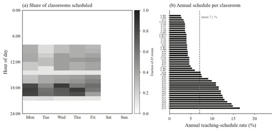
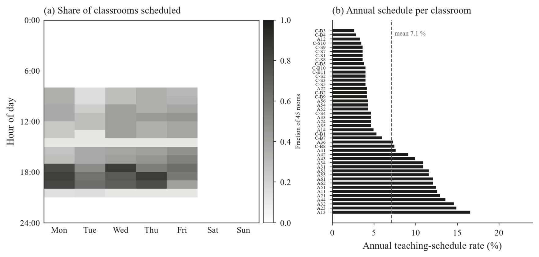
Teaching was timetabled on weekdays only, between 08:00 and 21:00, with 98.5% of the scheduled room-hours falling between 08:00 and 20:00. Overlapping the 45 classroom timetables in Figure 5a shows how scheduled teaching is distributed across the week. Within the 08:00–20:00 weekday window, one third of the available classroom-hours were assigned on average, but the assigned hours were concentrated rather than uniform: at the 17:00 peak, 84.4% of the 45 classrooms were timetabled simultaneously, through the late morning the maximum was below 40%, and at 14:00 no more than 5.6% were timetabled on any weekday. The union of the classroom timetables covers 1885 calendar hours (21.5% of the year).
Figure 5.
ETSAB classroom timetables for the 2025 reference week: (a) share of the 45 classrooms timetabled at each hour of the week and (b) annual teaching-schedule rate of each classroom (weekly scheduled hours × 29 teaching weeks/8760 h), ordered by rate, with the dashed line marking the mean (7.1%). Rates in (b) are shares of the 8760 annual hours.
The rate varied substantially among rooms. Across the 29 teaching weeks (145 teaching weekdays), annual teaching-schedule rates ranged from 2.6% to 16.6% of all the year’s hours, with a mean of 7.1%, or about 620 scheduled hours per room (Figure 5b, Appendix B). Reported separately, the Segarra classrooms were timetabled for 9.2% of annual hours on average and the Coderch classrooms for 4.1%. Against the 48.2% of the year in which the building was accessible, a single classroom was therefore assigned for roughly a seventh (15%) of that time.
3.2.2. Electricity Consumption by Schedule-Defined State at the Case Study Level
Over the 8760 calendar hours of 2025, 8552 h were successfully recorded (770 MWh, 97.6% of the year) and 208 were missed or invalid (2.4% of the year). The three states are divided as follows (Table 4, Figure 6):
Table 4.
ETSAB’s recorded 2025 electricity consumption classified by building access and classroom timetable. Mean values are W/m2 per observed hour of the state. The three states are mutually exclusive.
Figure 6.
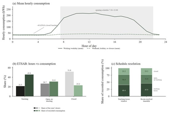
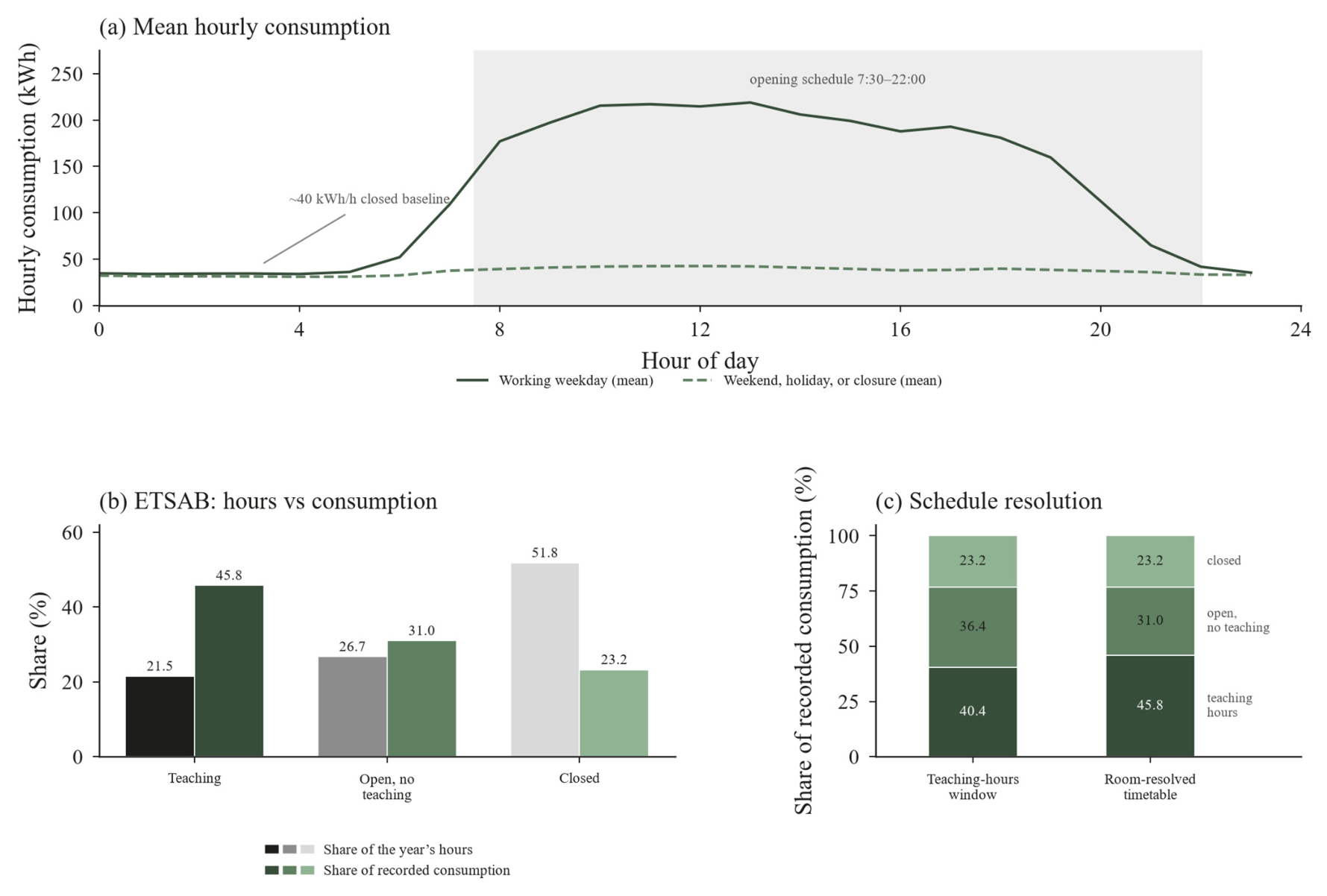
ETSAB electricity consumption in 2025: (a) mean hourly profiles on working weekdays and on weekends, holidays and closure days, with the weekday opening schedule shaded; (b) share of the year’s hours and of electrical consumption, with the unrecorded share shown in white; (c) consumption share under the teaching-hours window against the room-resolved timetable.
- (a)
- At least one classroom was timetabled during 1885 calendar hours (21.5% of the year; corresponding to 1836 valid metered hours and 49 invalid hours), carrying 45.8% of recorded electricity consumption (352 MWh).
- (b)
- The building was open with no classroom timetabled during 2340 calendar hours (26.7% of the year; corresponding to 2285 valid metered hours and 55 invalid hours), carrying 31.0% of recorded consumption (239 MWh).
- (c)
- Closed hours covered 4535 calendar hours (51.8% of the year; corresponding to 4431 valid metered hours and 104 invalid hours), and carried 23.2% of recorded consumption (179 MWh).
Mean consumption intensity was (a) 5.0 W/m2 during teaching hours, (b) 2.7 W/m2 during open hours without a timetabled classroom and (c) 1.1 W/m2 during closed hours. Taken together, 54.2% of recorded electrical consumption occurred with no classrooms timetabled or with the building closed.
The three states therefore separate physically as well as administratively, and in that order, but a base consumption of about 1.1 W/m2 persists through half of the year. The open state without a timetabled classroom is not idle time: it contains office work, the library, study rooms, model-making rooms, events and informal presence, as well as any base load. The library lies inside the metered boundary here, as it does at every other center, so the comparison between meters is unaffected. The meter cannot distinguish among these activities.
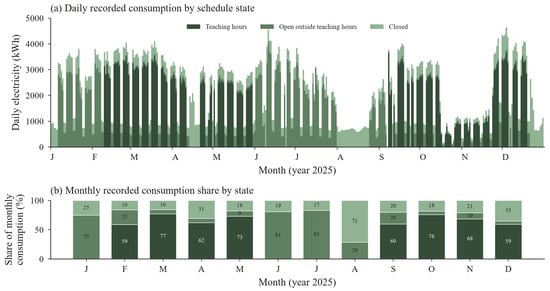
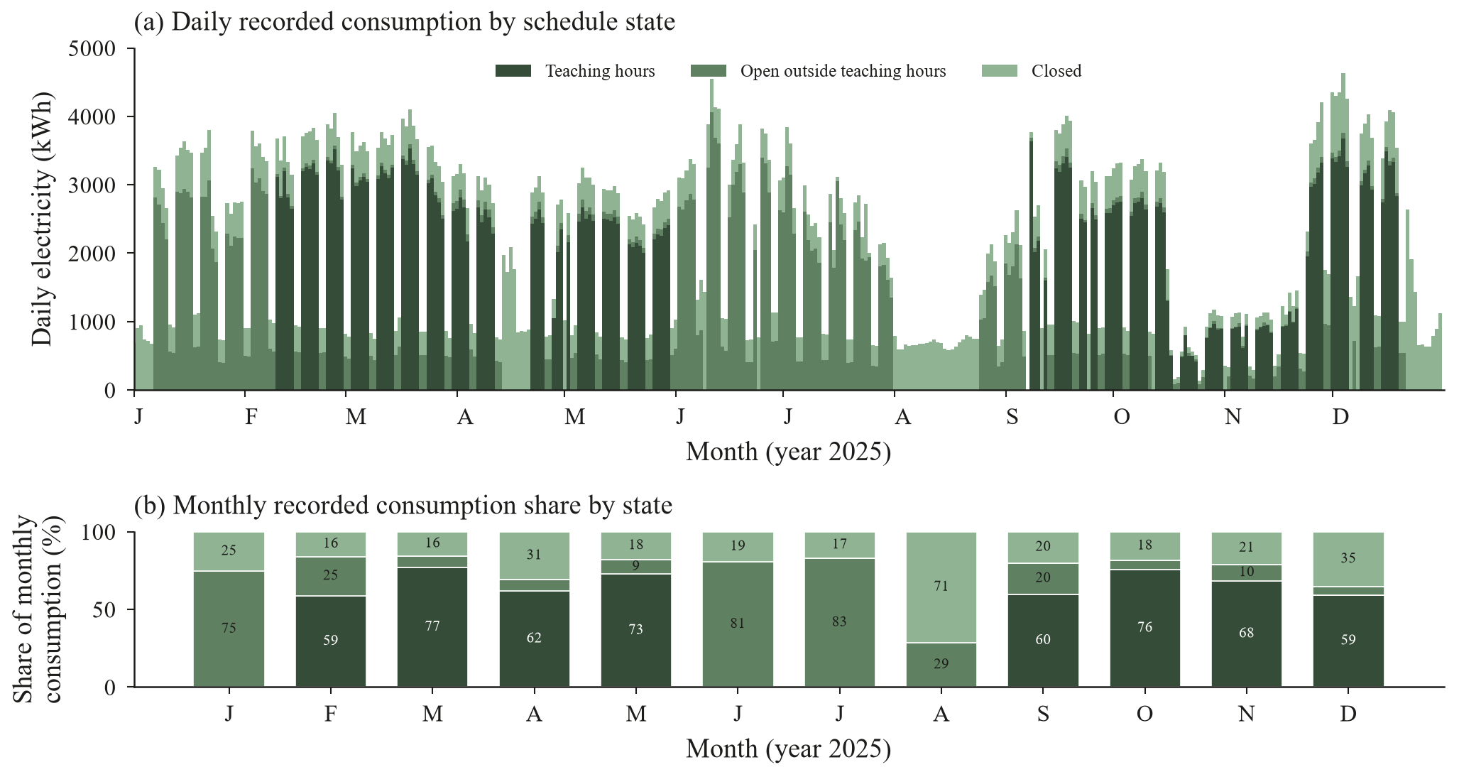
A day-level analysis shows that the daily minimal electricity consumption is insensitive to the length of the closure. During the August closure, the electricity consumption mean remained about 22 Wh/m2 per day and during the Christmas closure about 20 Wh/m2 per day, that is 29% and 27% of the working-weekday mean, although the two periods differ in duration and in outdoor conditions (Figure 7b).
Figure 7.
ETSAB daily electricity consumption in 2025: (a) daily consumption decomposed by schedule-defined state, with unrecorded hours shown in white; (b) monthly share of consumption by state.
3.3. Seasonal Analysis
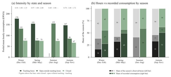
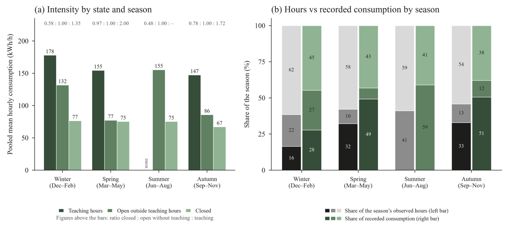
Grouping the observed hours by meteorological season shows that state intensities and their ratios vary across the year at the ten metered university buildings (Figure 8). The pooled seasonal ratio is 0.58 : 1 : 1.35 in winter (77, 132 and 178 kWh/h), 0.97 : 1 : 2.00 in spring (75, 77 and 155 kWh/h) and 0.78 : 1 : 1.72 in autumn (67, 86 and 147 kWh/h), around the annual 0.57 : 1 : 1.20. In summer (June–August), no generic teaching hours are scheduled and buildings close completely in August. During the open hours without teaching in June and July, however, the mean intensity is 155 kWh/h across the stock, values comparable to teaching-hour intensities in spring and autumn.
Figure 8.
Schedule-defined states by meteorological season across the ten classified meters: (a) pooled mean hourly consumption by state, with the ratio closed : open without teaching : teaching above each group; (b) share of observed hours (left bar) and of recorded consumption (right bar) in each state.
3.4. Effect of Schedule Resolution on the Electricity Classification (Generic Building Schedule vs. Per-Classroom Schedule)
ETSAB is used as a comparison case study since it has been classified under both constructs (general teaching schedule and detailed per-classroom schedule). On recorded consumption (770 MWh), the teaching-hours window (8:30–20:00) assigns 40.4% of the annual electricity consumption to (a) teaching hours and 36.4% to (b) open hours outside them, whereas the per-classroom timetables assign 45.8% to (a) hours with at least one classroom timetabled and 31.0% to (b) open hours with none. The window therefore displaces 5.4 percentage points of recorded consumption between the two open states under the start-of-hour convention for hour classification (Appendix C evaluates the effect of including the 8:30 boundary hour). The (c) closed state remains unchanged, since both classifications have the exact same closure times (Figure 6c).
In hours rather than in energy, the divergence is larger: the teaching hours count (a) 18.2% as teaching hours against (b) 21.5% with at least one classroom timetabled, because a window that is uniform across the day cannot reproduce the dense evening peak and the midday trough shown in Figure 5a. The general university-level analysis in Section 3.1 should therefore be read as correct to the order of magnitude of the split between the three states, but not as room-resolved results; only ETSAB is resolved at the room level.
3.5. Weekly Profile Shape: General Teaching Window Versus Classroom Timetables
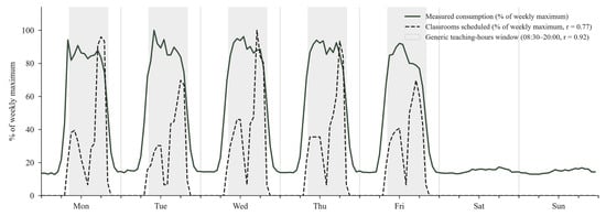
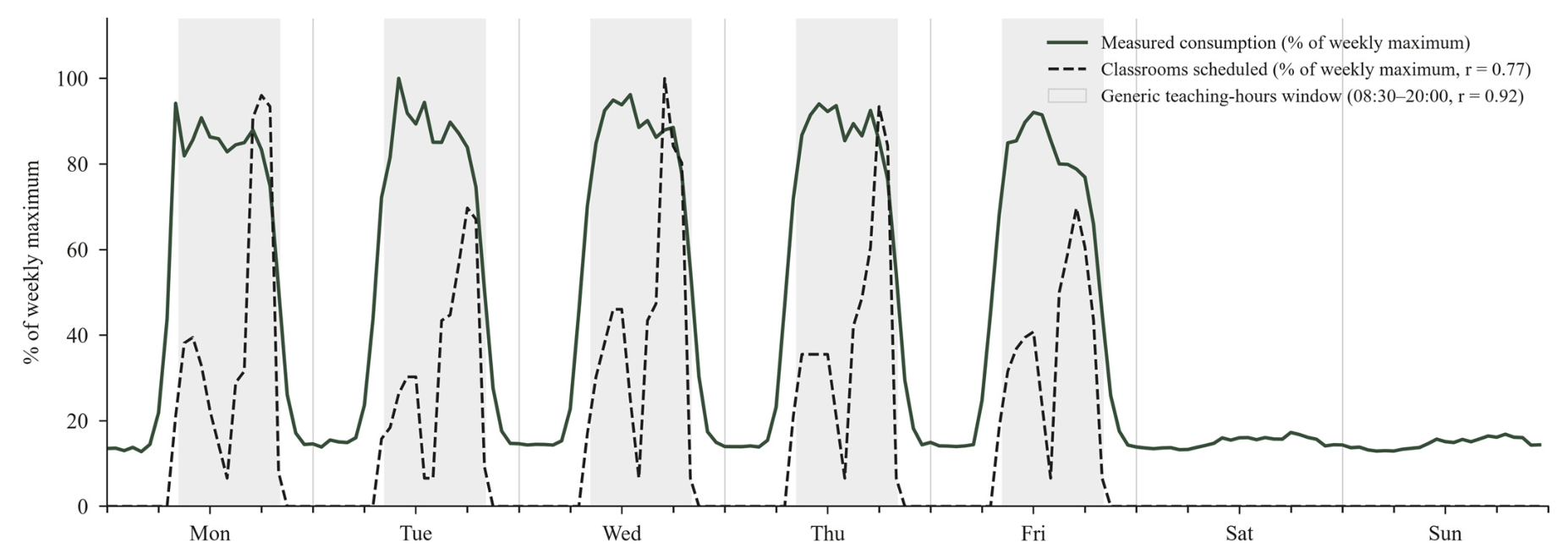
Figure 9 compares ETSAB’s mean hourly electricity profile across the teaching weeks of 2025 against the three schedule representations over the full 168 h week (Monday to Sunday). The classroom timetable varies sharply within each weekday, dropping to almost no rooms at midday (14:00) and peaking in the late afternoon (17:00–18:00). Measured whole-building electricity does not follow those intra-day swings: on every weekday it rises when the building opens, holds a largely flat daytime plateau across the entire generic teaching-hours window (08:30–20:00), and returns to the nighttime baseload at closing. At 14:00, when almost all classrooms are between lectures, building demand scarcely dips, because shared services, offices, studios, the bar, and the library continue operating through the lunch break and students remain in common areas rather than leaving the building. On weekends, the pattern reverses: although the building opens for study-room service (09:00–22:00), demand stays close to the closed baseline because lecture spaces and main building services remain closed.
Figure 9.
Mean weekly electricity consumption profile at ETSAB across the 2025 teaching weeks (168 h, Monday to Sunday) compared against the generic daily teaching-hours window (08:30–20:00 Monday–Friday, r = 0.92) and the scheduled classroom fraction (r = 0.77), each normalized to its weekly maximum.
Consequently, across the 168 h of the teaching week, the mean consumption profile correlates most strongly with the generic daily teaching-hours window (r = 0.92), ahead of the hour-by-hour fraction of scheduled classrooms (r = 0.77) and the opening schedule (r = 0.67). At the whole-building scale, electricity demand responds to whether the school is in its daily teaching regime rather than to how many classrooms are scheduled at each individual hour.
4. Discussion
4.1. Opening and Teaching Schedules Are Not Interchangeable
The principal finding of this paper is that opening schedules (when the building is accessible) and teaching schedules (when classrooms are planned to host lessons) are not interchangeable, and this is especially relevant in energy modeling. At the building level, the ETSAB case study was accessible during 48.2% of the year’s calendar hours, while at least one of its classrooms was timetabled during 21.5%, so the access schedule exceeds the assigned teaching state by a factor of about 2.3. At the room level, an individual classroom was timetabled for a mean of 7.1% of annual hours, while the building remained accessible for 48.2% (about a seventh of the accessible time). The two statements are not interchangeable, and neither converts into the other: one describes a whole building and the other a single room, and an energy model should use whichever matches the zone it represents.
At the whole-building level, the difference between schedules is mainly about how long each state lasts and which days it covers, rather than the hour-by-hour pattern of the classroom timetable within a day. Although the classroom timetable peaks at 84.4% in the early evening and falls to 5.6% at 14:00, whole-building electricity forms a daytime plateau across the weekday teaching window and correlates more strongly with the general daily teaching schedule (r = 0.92) than with the hour-by-hour fraction of scheduled classrooms (r = 0.77, Section 3.5). The intra-day timetable shape and the per-room spread (2.6% to 16.6% across the year) matter instead for room- and zone-level model inputs (internal gains, ventilation demand, and zone set-back), where one uniform schedule applied to all teaching zones misrepresents both tails of the distribution, in opposite directions. Neither schedule is a measurement of physical presence.
4.2. Electricity Consumption Associated with Temporal Conditions
Electricity consumption remained substantial outside the teaching hours, in every analyzed meter. Across the ten classified meters, 69.0% of recorded consumption (about 6.1 GWh of the 8.8 GWh recorded total) occurred outside the teaching-hours window, divided between (b) open hours outside teaching hours (27.2%, about 2.4 GWh) and (c) closed hours (41.8%, about 3.7 GWh).
At ETSAB, where the timetables permit greater resolution, 54.2% of recorded consumption occurred when (b) none of the classrooms was timetabled (31.0%) or (c) the building was closed (23.2%). Across the ten meters, closed hours represented 23.2–51.9% of each meter’s recorded annual consumption, while teaching hours carried 28.5–40.4%.
These shares are not estimates of potential energy consumption reduction. Servers, standby loads, lifts, minimum and emergency lighting, security and access-control systems, IT and wireless network equipment, telecommunication systems, laboratories, offices, the library, the bar, and other services do not follow classroom timetables, and administrative working hours are set by their own regulatory framework rather than by the academic calendar. With a single whole-building meter per center, the contribution of individual systems to the closed-hour baseload cannot be separated. The seasonal breakdown (Section 3.3, Figure 8) shows that state intensities and their ratios vary across the year, so the annual 0.57 : 1 : 1.20 scale is an average over seasons rather than a constant. In summer, no generic teaching hours are scheduled, and all buildings close completely during August (when consumption drops to the closed baseload), yet during open hours in June and July, mean hourly consumption across the stock is comparable to teaching-hour intensity in spring and autumn. Because multiple factors change simultaneously in summer (fewer students, higher space-cooling loads, and closures) whole-building meter data cannot isolate individual causes. A causal estimate of avoidable consumption would require sub-metered end uses or an operational intervention; the present result states the observed seasonal and state intensities as a factual baseline.
4.3. Comparison with Previous Studies
Three comparisons place this study in context. The first concerns out-of-hours consumption: one year of sub-metered data from an educational building in Melbourne attributes 48% of annual energy to non-working hours, with the mechanical system and plug loads reported to continue running on the weekday operating schedule during holiday closures when the building was empty [16]. In the ten classified meters in this study, between 23.2 and 51.9% of the recorded electricity consumption happened in closed hours. Our closed category is narrower than Melbourne’s non-working hours, because our buildings remain open into the evening and offer weekend study service. And even so, the highest value in the range (51.9%, at EEBE) already reaches their reported 48%.
The second concerns deviation from normative schedules. In offices, occupancy measured by motion sensors deviates by up to 46% from the values established in energy-code guidance [20]. The divergence between access-based and timetable-based schedule durations in educational buildings is likewise substantial, as the academic calendar removes a large fraction of the year and concentrates lectures into specific time windows.
The third concerns the relation between occupancy and metered energy. WiFi-derived occupancy on a university campus tracked metered electricity moderately well but HVAC operation only weakly [19]. In one university building, published room timetables for six teaching rooms compared with half-hourly electricity showed demand not strongly connected to the timetabled pattern [18]. The results reported here agree in direction, over a full calendar year, across ten meters covering twelve centers, with access separated from teaching schedules, and show further that whole-building electricity tracks the general daily teaching window rather than the hour-by-hour classroom timetable fraction.
4.4. Implications for Energy Modeling and Management
Opening schedules should not be used as proxies for occupancy in energy models. At the building level in the case studied here, the opening schedule exceeds the union of classroom timetables by a factor of 2.3, whereas at the room level an individual classroom is scheduled for only about a seventh of the time the building is accessible. Our weekly shape analysis (Section 3.5) refines how schedules should be matched to the spatial resolution of a model: for whole-building electricity analysis, the general daily teaching-hours schedule is more closely aligned with metered demand (r = 0.92) than either the opening schedule (r = 0.67) or the hour-by-hour classroom timetable fraction (r = 0.77).
The impact of switching from generic schedules to room-resolved timetables in dynamic energy simulation was quantified for this same school in a companion study [25]: in the detailed ETSAB simulation model, replacing generic schedules with timetable-based schedules changed simulated annual energy demand by +9% under manual solar-protection control, +6% under automatic control, and +0.5% under hybrid control.
For operations and space management, the results separate two questions that are often merged. How long buildings stay open relative to assigned teaching is a policy question, and this study indicates that this is where the variation lies, since the teaching-hours schedule varies by about three percentage points across centers, while opening schedules vary by almost twenty-two. Which systems continue to operate during those hours is an end-use question that building managers and operations should carefully assess. Consolidating timetables, shortening opening hours or choosing the right control systems may be worth investigating to reduce energy consumption.
4.5. Limitations
The university buildings analyzed here have a main educational use, combined with offices, library, study rooms, events and other informal uses that fall outside the timetable analysis while remaining inside the electricity meter boundary. This means that it is not possible to report specific per-user consumptions, so values reported here are per building. Room timetables are available for ETSAB only and represent a single mid-term reference week projected over the 29.0 teaching weeks (145 teaching weekdays) of 2025. The dedicated examination weeks of January and June are classified as open hours without teaching. The annual rate represents assigned time, not physical presence.
At the stock level, the teaching-hours window is a rough approximation whose boundaries rest on published sources (Appendix A). The sensitivity to the partial-hour (e.g., 8:30) boundary discretization in the electrical meter data classification is analyzed in Appendix C. Some meters aggregate several buildings and shared services for EETAC + EEABB and FME + CFIS. ETSEIB (27.1% missing winter and spring hours) and EPSEVG (on-site photovoltaic distortion) were excluded so that all ten retained meters have ≥97.6% valid coverage. Absolute intensities are not compared between centers because floor area, laboratory intensity, equipment and on-site photovoltaic generation largely differ between buildings. All consumption comparisons at different periods are descriptive and identify neither avoidable consumption nor causal effects.
Finally, the empirical shares and intensity ratios reported here derive from a single university in a Mediterranean climate with mixed teaching, research and administrative buildings. The method in this study transfers easily to future works, whereas the numerical values are specific to this case study.
5. Conclusions
Opening hours cannot be used as a proxy for teaching activity, especially at the classroom scale. Building access and scheduled teaching represent fundamentally different operational states. Treating a building’s opening schedule as its active occupancy schedule severely overstates active duration at the whole-building level and completely misrepresents utilization at the individual classroom level.
University electricity demand is driven primarily by generic teaching schedules rather than scheduled per-classroom teaching. Because baseline loads during closed hours and non-teaching open hours remain high relative to teaching hours, most annual electricity consumption occurs outside scheduled teaching windows. Scheduled classes add only a moderate incremental load on top of the energy already required simply to keep the building open and running.
At the whole-building level, a general daily teaching window is sufficient and tracks metered electricity better than granular classroom timetables. Because whole-building demand stays on a flat plateau throughout weekday teaching hours (even during the 14:00 lunch dip when almost no classes are scheduled) and stays near the closed baseload during weekend study-room openings, hourly building consumption follows the binary daily teaching regime (r = 0.92) more closely than the hour-by-hour fraction of scheduled classrooms (r = 0.77).
Author Contributions
Conceptualization, M.R.-M., I.C.-C. and H.C.; methodology, M.R.-M., I.C.-C. and H.C.; software, M.R.-M.; validation, M.R.-M., I.C.-C. and H.C.; formal analysis, M.R.-M.; investigation, M.R.-M.; resources, I.C.-C. and H.C.; data curation, M.R.-M.; writing—original draft preparation, M.R.-M.; writing—review and editing, I.C.-C. and H.C.; visualization, M.R.-M.; supervision, I.C.-C. and H.C.; project administration, I.C.-C. and H.C.; funding acquisition, I.C.-C. and H.C. All authors have read and agreed to the published version of the manuscript.
Funding
This work was carried out by the project DOM-P “Dynamic Occupancy Management of Well-Being for People” (PID2024-156720OB-I00), funded by MICIU/AEI/10.13039/501100011033 and FEDER, EU.
Data Availability Statement
Classroom timetables were derived from the public ETSAB “occupancy per classroom” service and from the UPC academic calendar. Hourly electricity was exported from Sirena, UPC’s centralized monitoring platform, and is available from the corresponding author on request. Building access schedules were collected from the official center and campus sources listed in Appendix A.
Acknowledgments
In the data analysis, the authors used generative AI models SWE-2.0, OpenAI GPT-5.6-Sol and Anthropic Claude Fable 5.1 from Devin AI (Cognition) for code drafting. The authors have reviewed and edited the output and take full responsibility.
Conflicts of Interest
The authors declare no conflicts of interest.
Abbreviations
The following abbreviations are used in this manuscript:
| UPC | Universitat Politècnica de Catalunya · BarcelonaTech (Polytechnic University of Catalonia) |
| ETSAB | Barcelona School of Architecture |
| EPSEB | Barcelona School of Building Construction |
| FME | School of Mathematics and Statistics |
| ETSEIB | Barcelona School of Industrial Engineering |
| ETSECCPB | Barcelona School of Civil Engineering |
| EETAC | Castelldefels School of Telecommunications and Aerospace Engineering |
| EEABB | Barcelona School of Agri-Food and Biosystems Engineering |
| ESEIAAT | Terrassa School of Industrial, Aerospace and Audiovisual Engineering |
| EPSEM | Manresa School of Engineering |
| CFIS | Interdisciplinary Higher Education Center |
| ETSETB | Barcelona School of Telecommunications Engineering |
| EEBE | Barcelona East School of Engineering |
| FIB | Barcelona School of Informatics |
| FNB | Barcelona School of Nautical Studies |
| ETSAV | Vallès School of Architecture |
| FOOT | Terrassa School of Optics and Optometry |
| CITM | Image Processing and Multimedia Technology Center |
| EPSEVG | Vilanova i la Geltrú School of Engineering |
| AI | Artificial intelligence |
| AiEM | Arquitectura, Energia i Medi Ambient |
| HVAC | Heating, ventilation and air conditioning |
Appendix A. Access-Schedule per Center
Table A1 records, for each of the eighteen UPC teaching centers, the source of its published access schedule, the type of evidence (official building-hours page, access-calendar document, business listing or direct enquiry), the consultation date, the weekday and weekend access windows, and the documented closure periods used in the classification.
Table A1.
Opening windows of the eighteen UPC centers.
Appendix B. Annual Teaching-Schedule Rate of ETSAB
Table A2.
Annual teaching-schedule rate of each of the 45 ETSAB classrooms, ordered by rate and identified by building.
Appendix C. Sensitivity to Half-Hour (0:30) Schedule Boundaries
Hourly electricity records are stamped at the start of each hour (00:00 to 23:00) and are indivisible. When a published opening or teaching-window boundary falls on a half-hour (such as 07:30 for weekday opening or 08:30 for the start of the generic teaching window at ETSAB, EEBE and ETSAV), the main analysis assigns each whole-hour record according to the schedule status at the start of the hour (strict start-of-hour rule), so a 07:30 opening takes effect at 08:00 and a 08:30 teaching start takes effect at 09:00. To bound the discretization effect of whole-hour assignment, Table A3 compares the strict start-of-hour rule against an inclusive overlap rule in which any whole hour partially overlapping a schedule window (such as 07:00–08:00 for a 07:30 opening or 08:00–09:00 for a 08:30 teaching start) is included in that state.
Across the three centers whose generic teaching window starts at 08:30, including the 08:00–09:00 edge hour increases the annual teaching-window hour share ((a) %h) from 18.2% to 19.9% at ETSAB (midpoint 19.0 ± 0.8%, matching the continuous duration 11.5 h × 145 d/8760 h = 19.0%) and from 20.0% to 21.7% at EEBE and ETSAV (midpoint 20.8 ± 0.8%, matching 12.5 h × 146 d/8760 h = 20.8%), and shifts (a) %kWh by +3.2 percentage points at ETSAB (40.4% to 43.6%), +2.3 percentage points at EEBE (29.1% to 31.4%) and +2.5 percentage points at ETSAV (34.1% to 36.6%). Consequently, in Section 3.4 the difference at ETSAB between the room-resolved timetable (45.8% of recorded consumption in (a)) and the generic teaching-hours window ranges from 5.4 percentage points under the strict rule to 2.2 percentage points under the inclusive rule (3.8 ± 1.6 percentage points). Pooled across all ten meters, the two rules yield nearly identical stock totals (31.0/27.2/41.8% versus 32.3/29.2/38.5% of recorded consumption, or 69.0% versus 67.7% outside teaching) and pooled intensity ratios (0.57 : 1 : 1.20 versus 0.56 : 1 : 1.25).
Table A3.
Sensitivity of schedule-state hour shares (%h of 8760 h) and recorded electricity shares (%kWh of recorded consumption) to the half-hour boundary assignment rule across the ten classified meters. Each cell reports midpoint ± half-range between the strict start-of-hour rule and the inclusive-overlap rule. ± 0.0 marks states whose windows contain no half-hour boundary.
References
- Ministerio de Transportes, Movilidad y Agenda Urbana de España Código Técnico de la Edificación; Agencia Estatal Boletín Oficial del Estado: Madrid, Spain, 2021.
- Hoes, P.; Hensen, J.L.M.; Loomans, M.G.L.C.; de Vries, B.; Bourgeois, D. User Behavior in Whole Building Simulation. Energy Build. 2009, 41, 295–302. [Google Scholar] [CrossRef] [Scilit]
- Yang, Z.; Becerik-Gerber, B. How Does Building Occupancy Influence Energy Efficiency of HVAC Systems? Energy Procedia 2016, 88, 775–780. [Google Scholar] [CrossRef] [Scilit]
- Oldewurtel, F.; Sturzenegger, D.; Morari, M. Importance of Occupancy Information for Building Climate Control. Appl. Energy 2013, 101, 521–532. [Google Scholar] [CrossRef] [Scilit]
- Menezes, A.C.; Cripps, A.; Bouchlaghem, D.; Buswell, R. Predicted vs. Actual Energy Performance of Non-Domestic Buildings: Using Post-Occupancy Evaluation Data to Reduce the Performance Gap. Appl. Energy 2012, 97, 355–364. [Google Scholar] [CrossRef] [Scilit]
- Jia, M.; Srinivasan, R.S.; Raheem, A.A. From Occupancy to Occupant Behavior: An Analytical Survey of Data Acquisition Technologies, Modeling Methodologies and Simulation Coupling Mechanisms for Building Energy Efficiency. Renew. Sustain. Energy Rev. 2017, 68, 525–540. [Google Scholar] [CrossRef] [Scilit]
- Hong, T.; Yan, D.; D’Oca, S.; Chen, C. Ten Questions Concerning Occupant Behavior in Buildings: The Big Picture. Build. Environ. 2017, 114, 518–530. [Google Scholar] [CrossRef] [Scilit]
- van Dronkelaar, C.; Dowson, M.; Spataru, C.; Burman, E.; Mumovic, D. Quantifying the Underlying Causes of a Discrepancy Between Predicted and Measured Energy Use. Front. Mech. Eng. 2019, 5, e00020. [Google Scholar] [CrossRef] [Scilit]
- Page, J.; Robinson, D.; Morel, N.; Scartezzini, J.-L. A Generalised Stochastic Model for the Simulation of Occupant Presence. Energy Build. 2008, 40, 83–98. [Google Scholar] [CrossRef] [Scilit]
- Yan, D.; Hong, T.; Dong, B.; Mahdavi, A.; D’Oca, S.; Gaetani, I.; Feng, X. IEA EBC Annex 66: Definition and Simulation of Occupant Behavior in Buildings. Energy Build. 2017, 156, 258–270. [Google Scholar] [CrossRef] [Scilit]
- Park, J.Y.; Ouf, M.M.; Gunay, B.; Peng, Y.; O’Brien, W.; Kjærgaard, M.B.; Nagy, Z. A Critical Review of Field Implementations of Occupant-Centric Building Controls. Build. Environ. 2019, 165, 106351. [Google Scholar] [CrossRef] [Scilit]
- Happle, G.; Fonseca, J.A.; Schlueter, A. A Review on Occupant Behavior in Urban Building Energy Models. Energy Build. 2018, 174, 276–292. [Google Scholar] [CrossRef] [Scilit]
- Gaetani, I.; Hoes, P.-J.; Hensen, J.L.M. Occupant Behavior in Building Energy Simulation: Towards a Fit-for-Purpose Modeling Strategy. Energy Build. 2016, 121, 188–204. [Google Scholar] [CrossRef] [Scilit]
- Bourdeau, M.; Guo, X.; Nefzaoui, E. Buildings Energy Consumption Generation Gap: A Post-Occupancy Assessment in a Case Study of Three Higher Education Buildings. Energy Build. 2018, 159, 600–611. [Google Scholar] [CrossRef] [Scilit]
- Khoshbakht, M.; Gou, Z.; Dupre, K. Energy Use Characteristics and Benchmarking for Higher Education Buildings. Energy Build. 2018, 164, 61–76. [Google Scholar] [CrossRef] [Scilit]
- Alam, M.; Devjani, M.R. Analyzing Energy Consumption Patterns of an Educational Building through Data Mining. J. Build. Eng. 2021, 44, 103385. [Google Scholar] [CrossRef] [Scilit]
- García-Monge, M.; Zalba, B.; Casas, R.; Cano, E.; Guillén-Lambea, S.; López-Mesa, B.; Martínez, I. Is IoT Monitoring Key to Improve Building Energy Efficiency? Case Study of a Smart Campus in Spain. Energy Build. 2023, 285, 112882. [Google Scholar] [CrossRef] [Scilit]
- Gul, M.S.; Patidar, S. Understanding the Energy Consumption and Occupancy of a Multi-Purpose Academic Building. Energy Build. 2015, 87, 155–165. [Google Scholar] [CrossRef] [Scilit]
- Martani, C.; Lee, D.; Robinson, P.; Britter, R.; Ratti, C. ENERNET: Studying the Dynamic Relationship between Building Occupancy and Energy Consumption. Energy Build. 2012, 47, 584–591. [Google Scholar] [CrossRef] [Scilit]
- Duarte, C.; Van Den Wymelenberg, K.; Rieger, C. Revealing Occupancy Patterns in an Office Building through the Use of Occupancy Sensor Data. Energy Build. 2013, 67, 587–595. [Google Scholar] [CrossRef] [Scilit]
- Bae, Y.; Yoon, Y.; Jung, S.; Malhotra, M.; Im, P. Occupancy Schedule Development and Its Effect on OpenStudio Prototype College Building Model. Sci. Technol. Built Environ. 2024, 30, 287–301. [Google Scholar] [CrossRef] [Scilit]
- Al-Saegh, S.; Kourgiozou, V.; Korolija, I.; Tang, R.; Tahmasebi, F.; Mumovic, D. Investigating Building Stock Energy and Occupancy Modelling Approaches for District-Level Heating and Cooling Energy Demands Estimation in a University Campus. Energy Build. 2025, 329, 115269. [Google Scholar] [CrossRef] [Scilit]
- Davis, J.A.; Nutter, D.W. Occupancy Diversity Factors for Common University Building Types. Energy Build. 2010, 42, 1543–1551. [Google Scholar] [CrossRef] [Scilit]
- Alfalah, B.; Shahrestani, M.; Shao, L. Identifying Occupancy Patterns and Profiles in Higher Education Institution Buildings with High Occupancy Density—A Case Study. Intell. Build. Int. 2023, 15, 45–61. [Google Scholar] [CrossRef] [Scilit]
- Roca-Musach, M. Automatismes, Usuaris i Arquitectura: Aplicació a la Gestió Energètica dels Edificis. Ph.D. Thesis, Universitat Politècnica de Catalunya, Barcelona, Spain, 2024. [Google Scholar]
- Ministerio de Hacienda y Función Pública de España Cadastral Electronic Site. Available online: https://www.sedecatastro.gob.es/ (accessed on 3 October 2022).
- ETSAB Occupancy per Classroom. Available online: https://etsab.upc.edu/ca/serveis-ab/reserva_despais/ocupacio-aules/ocupacio-per-aula (accessed on 17 September 2026).

Disclaimer/Publisher’s Note: The statements, opinions and data contained in all publications are solely those of the individual author(s) and contributor(s) and not of MDPI and/or the editor(s). MDPI and/or the editor(s) disclaim responsibility for any injury to people or property resulting from any ideas, methods, instructions or products referred to in the content. |
© 2026 by the authors. Licensee MDPI, Basel, Switzerland. This article is an open access article distributed under the terms and conditions of the Creative Commons Attribution (CC BY) license.