


Abstract
This study addresses the multi-objective trade-off between daylight utilization and reductions in the annual spatial-mean DGP indicator in office spaces in cold regions. A parametric daylight optimization framework was developed for a typical side-lit office in Lanzhou, using window-to-wall ratio (WWR), window aspect ratio (AR), external shading depth (SD), and building orientation (ORI) as design variables, and useful daylight illuminance (UDI), spatially averaged point-based daylight autonomy (mean DA), and annual spatial-mean daylight glare probability (DGP) as performance metrics. First, 500 baseline full-factorial simulations were conducted, and multifactor analysis of variance was used to quantify the relative contributions of the design variables and their two-factor interactions to the modeled response variation within the predefined full-factorial design domain. Second-order response surface surrogate models were then established separately for four orientations and validated using 48 independent off-grid samples. NSGA-II was subsequently employed to identify three-objective Pareto fronts, while TOPSIS was used to select representative solutions under different performance preferences. Within the investigated baseline full-factorial design domain, WWR showed the largest relative contribution to the model-explained variation in UDI and mean DA, accounting for 69.48% and 58.26%, respectively, whereas ORI showed the largest relative contribution to the annual spatial-mean DGP response, accounting for 56.20%. High-ranking Pareto solutions within the baseline design domain cluster near the upper bounds of WWR and AR, indicating that fixed rectangular bounds may truncate potentially high-performing regions. To examine this boundary effect, 48 geometry-constrained extended-domain training samples and 24 independent validation samples were introduced, with optimization restricted to the actual training-data coverage and a 0.30 m window-edge geometric constraint. Within the investigated simulation-supported extended domain, the maximum UDI and mean DA were higher than their baseline-domain extrema by approximately 2.4–3.9 and 7.1–8.6 percentage points, respectively, while the minimum values of the annual spatial-mean DGP indicator were approximately 32–47% lower under the specified simulation conditions. To further assess optimization reliability, 20 additional Pareto candidates were re-simulated, showing within-orientation ranking agreement of 92.5% for UDI and 100% for both mean DA and the annual spatial-mean DGP indicator. Distinct window–shading trade-offs were observed among the objectives: higher mean DA favored larger transparent openings with shallow shading, lower annual spatial-mean DGP values favored smaller WWRs with deeper shading, whereas higher UDI depended more strongly on a compensatory coupling between larger windows and stronger shading. Overall, the proposed framework reveals orientation-dependent performance trade-offs across a broader design space while controlling surrogate-model extrapolation risk, providing a quantitative basis for early-stage parametric fenestration design in office buildings.
1. Introduction
Against the backdrop of the global transition toward low-carbon buildings, improving environmental performance during building operation through passive design remains of continuing importance [1,2,3]. In office buildings, daylight can improve the indoor visual environment and reduce the demand for artificial lighting, but excessive solar radiation and high-luminance windows may also lead to overexposure and visual discomfort due to glare [4,5,6]. Therefore, the primary objective of daylighting design is not simply to increase indoor illuminance, but rather to achieve an appropriate balance between daylight availability and overall visual comfort-related performance. Compared with static evaluations conducted at a single time point or under representative sky conditions, climate-based dynamic daylight metrics derived from annual weather data can provide a more comprehensive representation of luminous conditions under actual operating conditions [7,8]. Among these metrics, Useful Daylight Illuminance (UDI) and Daylight Autonomy (DA) respectively characterize the effective utilization of daylight and the extent to which a target illuminance level is achieved [9], while Daylight Glare Probability (DGP) provides a quantitative indicator related to glare potential caused by high-luminance windows and direct sunlight [10]. In the present study, however, the glare-related optimization objective is an annual spatial-mean DGP indicator obtained through spatial and temporal aggregation of hourly imageless DGP results; it is therefore used as a comparative annual response among design alternatives rather than as a direct measure of occupant-specific instantaneous glare risk. Taken together, these metrics provide complementary information on daylight quantity, effective daylight availability, and the annual glare-related response considered in this study. Building windows constitute a key interface between the outdoor luminous environment and the indoor visual environment, and their area, proportions, shading configuration, and orientation jointly affect annual daylighting performance. The Window-to-Wall Ratio (WWR) determines the area of the primary daylight opening and is one of the most extensively investigated parameters in daylighting and building-envelope design. Increasing WWR generally allows more daylight to enter the space and raises indoor daylight levels; however, larger transparent openings may also increase the likelihood of excessive exposure and glare in near-window zones [11]. In addition to window area, variations in window Aspect Ratio (AR), while maintaining a comparable opening area, alter the horizontal and vertical distribution of the opening on the facade as well as the path through which daylight penetrates deeper into the interior [12]. External Shading Depth (SD), meanwhile, influences the trade-off between daylight availability and the annual spatial-mean DGP response considered in this study by modifying direct solar exposure and the visible sky component [13]. At the same time, building orientation (ORI) alters the timing and intensity of incident solar radiation, causing identical window–shading configurations to produce different responses on different facades [14]. Accordingly, WWR, AR, SD, and orientation categories should not be regarded as independent parameters; instead, their main effects and interactions may jointly govern annual daylighting performance.
Advances in parametric modeling and building performance simulation have made it possible to generate and evaluate large numbers of fenestration and shading configurations [15,16]. However, directly using high-fidelity simulation tools such as Radiance throughout the entire optimization process remains computationally expensive. Moreover, evaluating only a limited number of discrete design alternatives makes it difficult to identify nonlinear relationships and interactions among multiple design parameters. Surrogate models have therefore been widely adopted to accelerate building-performance prediction and optimization, although their reliability should be assessed using independent validation and, where optimization preferentially explores extreme or boundary regions, additional high-fidelity confirmation rather than fitting accuracy alone [17,18]. Among these approaches, Response Surface Methodology (RSM) can establish explicit mathematical mappings between design variables and performance metrics using a limited number of high-fidelity simulation samples [19]. In particular, second-order response surface models can construct continuous performance mappings from a relatively small number of simulation samples while explicitly representing linear, quadratic, and two-factor interaction terms, thereby providing good statistical interpretability. When combined with analysis of variance (ANOVA), the relative contributions of individual factors and their interactions to modeled response variation can be quantified within a predefined design-of-experiments domain, providing an interpretable description of parameter sensitivity that remains conditional on the selected factor levels and model structure.
Daylighting design for office spaces is also inherently a multi-objective problem [20,21,22,23,24]. Enlarging window openings or reducing shading can improve mean DA, but may simultaneously increase excessive daylight exposure and the annual glare-related response represented here by the annual spatial-mean DGP indicator. Conversely, stronger shading can reduce the annual spatial-mean DGP indicator but may also decrease daylight availability in deeper parts of the room [25,26,27]. It is therefore difficult to identify a single optimal design that satisfies all performance objectives using only one metric. Multi-objective algorithms in the NSGA family can characterize trade-offs among conflicting objectives through Pareto fronts [28,29,30], while multi-attribute decision-making methods such as the Technique for Order Preference by Similarity to Ideal Solution (TOPSIS) can further identify representative solutions from a set of non-dominated alternatives according to different design preferences [31].
Although previous studies have demonstrated the effectiveness of parametric simulation, surrogate modeling, and multi-objective algorithms for building daylighting optimization, several issues warrant further investigation. First, interactions among window area, window proportions, external shading, and orientation have not yet been systematically quantified, which limits the interpretation of multi-parameter coupling mechanisms. Second, for geometrically coupled variables such as WWR and AR, the use of mutually independent rectangular parameter bounds may constrain the actual feasible design space. This issue is particularly relevant in complete full-factorial experiments, where relatively conservative parameter ranges are often required to preserve both statistical balance and the geometric feasibility of all parameter combinations. When optimized solutions repeatedly cluster near predefined bounds, it becomes necessary to distinguish genuine performance-driven convergence from truncation imposed by artificial search boundaries. Third, although high-dimensional black-box surrogate models can achieve high predictive accuracy, their outputs are often difficult to translate directly into interpretable architectural design knowledge. A research framework is therefore needed that simultaneously considers statistical interpretability, geometric feasibility, surrogate-model reliability, and the efficiency of multi-objective optimization.
To address these issues, this study investigates a typical side-lit office space in a cold region and adopts Window-to-Wall Ratio (WWR), window Aspect Ratio (AR), external Shading Depth (SD), and building Orientation (ORI) as the principal design variables, with UDI, DA, and annual spatial-mean DGP serving as daylighting performance indicators. An integrated research framework is developed that links parametric modeling, climate-based daylight simulation, multi-objective optimization, and design decision-making. First, a baseline daylighting-performance database is established using a complete full-factorial design of experiments, while additional off-grid samples are reserved exclusively for independent validation; multifactor ANOVA is then used to decompose the modeled response variation into the relative contributions of the main effects and two-factor interactions within the predefined baseline design domain. Second, orientation-specific second-order response surface surrogate models are developed separately for UDI, mean DA, and annual spatial-mean DGP under each of the four predefined orientation scenarios and are evaluated using cross-validation and fully independent validation samples. Based on these models, NSGA-II is applied separately for each orientation to identify Pareto-optimal solutions within the validated baseline full-factorial design domain, with the objectives of improving UDI and mean DA while reducing the annual spatial-mean DGP indicator. TOPSIS is then used to select representative optimal solutions under different performance-weighting scenarios.
The study further introduces a geometry-constrained extended design domain as a boundary-sensitivity investigation to examine whether the original rectangular parameter bounds restrict the exploration of additional simulation-supported high-performing regions. Additional high-fidelity training and independent validation samples are introduced within the geometrically feasible region, while the subsequent surrogate-assisted optimization is restricted to the sampled training-data envelope to avoid unsupported extrapolation. Representative extreme-objective solutions obtained from the extended-domain Pareto sets are further re-evaluated using the original Honeybee simulation workflow to assess local predictive reliability in the regions preferentially explored by NSGA-II. Accordingly, the extended-domain analysis is not intended to identify an unrestricted global optimum or a universally complete architectural design space; rather, it is used to characterize boundary sensitivity, parameter migration, and performance trends within the current geometry- and data-supported domain. The resulting optimization outcomes are therefore interpreted as directional and range-based references for early-stage parametric design rather than as prescriptive fixed dimensions.
2. Materials and Methods
2.1. Research Framework and Parametric Building Model
This study establishes an office-space daylighting performance optimization framework integrating parametric modeling, sample design, climate-based daylight simulation, statistical analysis, surrogate model development, multi-objective optimization, and multi-level validation of surrogate predictions and optimization results. These components are interconnected to form a complete analytical workflow extending from design-parameter input and performance simulation to optimization and decision-making. The overall research framework is shown in Figure 1. The workflow consists of six sequential stages: (1) research object and parametric model definition, (2) parameter setting and sample generation, (3) climate-based daylight simulation, (4) statistical analysis, (5) surrogate model construction and validation, and (6) multi-objective optimization and confirmatory evaluation. First, a parametric model of a typical side-lit office space is developed in Rhinoceros 7 and Grasshopper. Window-to-Wall Ratio (WWR), window Aspect Ratio (AR), external Shading Depth (SD), and four predefined building-orientation categories (ORI) are selected as the principal design variables to characterize the combined relationships among fenestration geometry, shading dimensions, orientation, and indoor daylighting performance. A baseline full-factorial design domain and a geometry-constrained extended design domain are then established separately. In the baseline stage, a complete full-factorial experiment is conducted to quantify the effects of the design variables and their two-factor interactions on the daylighting performance metrics, while additional off-grid samples are used to evaluate the continuous predictive capability and local generalization performance of the surrogate models between the regular training-grid points. After completing multi-objective optimization within the baseline design domain, the boundary-concentration characteristics of the Pareto-optimal solutions along the WWR and AR dimensions are examined to determine whether the initial parameter bounds may restrict the exploration of additional geometrically feasible high-performing regions. On this basis, an extended design domain is constructed by introducing explicit window-opening geometric constraints together with additional high-fidelity daylight simulations. Independent validation samples are subsequently used to assess the external predictive capability of the reconstructed surrogate models within the extended domain before constrained multi-objective optimization is performed. After optimization, the maximum-UDI, maximum-mean-DA, and minimum-annual-spatial-mean-DGP solutions for each orientation were re-simulated using the original Grasshopper–Honeybee workflow. In addition, 20 Pareto candidates were selected from the extended-domain solution sets to examine prediction errors, relative rankings, and pairwise dominance relationships in selected multi-objective trade-off regions. Together, these confirmation simulations provided complementary assessments of surrogate-model performance at selected extreme solutions and across representative Pareto candidates.
Figure 1.
Research framework.
The parametric building model comprises modules for spatial geometry, fenestration geometry, external shading, orientation control, and Honeybee-based annual daylight and glare simulations using Radiance [32]. These modules are coordinately controlled through parametric associations in Grasshopper, as illustrated in Figure 2. The prototype office space has a width of 4.20 m, a depth of 7.50 m, and a height of 3.00 m, corresponding to a floor area of 31.50 m2. Additional geometric parameters, material properties, and daylight simulation settings are listed in Table 1, while the representative parametric building model is shown in Figure 3. Except for the four study variables—WWR, AR, SD, and ORI—all other spatial dimensions, envelope geometric properties, material optical properties, and simulation boundary conditions are kept constant across all cases to minimize the influence of non-study variables on performance comparisons. Specifically, WWR and AR jointly control the total fenestration area and window proportions, while SD regulates the horizontal projection depth of the external shading device. Building orientation is implemented by rotating the entire office space and its envelope model, with the rotation angle uniformly controlled by the ORI parameter, thereby ensuring consistent geometric relationships and simulation conditions across different orientation scenarios. The four ORI values were treated as predefined orientation categories rather than as a continuous angular predictor. In the Grasshopper model, the orientation angles were referenced to geographic south and increased counterclockwise, such that 0°, 90°, 180°, and 270° corresponded to south-, east-, north-, and west-facing facade orientations, respectively.
Figure 2.
Grasshopper parametric modeling and Honeybee simulation workflow of the prototype office and fenestration system.
Table 1.
Prototype office model, design variables, and simulation settings.
Figure 3.
Prototype office model and sensor-grid configuration: (a) simplified geometric model; (b) plan-view distribution of the 180 sensor points on the horizontal analysis plane at 0.80 m above the floor.
2.2. Design Parameters and Sample Generation
To establish a regular and balanced baseline dataset suitable for multifactor analysis of variance (ANOVA) and second-order response surface modeling, this study first constructs a baseline full-factorial design domain. It should be noted that WWR and AR are treated as two independent design variables in the statistical analysis, although they are geometrically coupled in the building model. Therefore, the baseline full-factorial domain should be interpreted as a statistically balanced exploration space rather than a complete representation of all physically feasible window configurations. Specifically, increasing WWR enlarges the total window-opening area, while AR further determines the vertical and horizontal dimensions of the opening. When a relatively large WWR is combined with a more extreme AR value, some parameter combinations may exceed the geometrically feasible range of the fixed facade. Because a complete full-factorial experiment requires a Cartesian product of all factor levels, relatively conservative fixed rectangular parameter bounds are adopted in the initial stage to maintain a balanced experimental structure while avoiding obviously infeasible window configurations. WWR is therefore set to 0.30–0.50 at five levels, AR to 0.40–1.20 at five levels, and SD to 0–1.20 m at five levels, while ORI is defined as four categorical orientation levels of 0°, 90°, 180°, and 270°, resulting in a balanced 5 × 5 × 5 × 4 full-factorial dataset comprising 500 simulation cases [33]. It should be emphasized that WWR = 0.50 and AR = 1.20 initially represent the search boundaries of the baseline full-factorial design rather than a priori physical optima or universally applicable design limits.
To avoid evaluating surrogate-model performance solely at the discrete levels of the regular full-factorial design, which would provide limited information on continuous interpolation capability, an additional set of 48 fully independent off-grid validation samples is generated within the baseline parameter ranges and excluded from surrogate-model fitting, parameter estimation, cross-validation, model selection, and hyperparameter adjustment. These samples are formed by combining 12 continuous WWR–AR–SD configurations with the four orientations. All parameter values remain within the baseline full-factorial domain but are deliberately positioned away from the principal discrete factor levels. Specifically, WWR ranges from 0.308 to 0.491, AR from 0.423 to 1.177, and SD from 0.082 to 1.108 m.
After completing the multi-objective optimization within the baseline design domain, representative solutions corresponding to three TOPSIS weighting scenarios—Equal, Daylight-Balanced, and Annual-DGP-Priority—are selected from the Pareto front for each of the four orientations. Three solutions are selected per orientation, yielding a total of 12 final confirmatory cases. These solutions are then reintroduced into the original Grasshopper–Honeybee model for full daylight simulations, and the simulated UDI, mean DA, and annual spatial-mean DGP values are compared with the corresponding surrogate-model predictions to assess local predictive reliability within the regions preferentially explored by NSGA-II.
The Pareto results obtained within the baseline design domain further show that high-ranking solutions for multiple orientations consistently cluster near the upper bounds of WWR and AR. Because these fixed upper limits were initially imposed in part to ensure the geometric feasibility of all combinations in the complete full-factorial design, such boundary concentration cannot be interpreted directly as evidence that WWR = 0.50 or AR = 1.20 is physically optimal. Instead, it indicates the need to examine whether the initial rectangular search domain truncates a broader geometrically feasible design space.
Accordingly, a geometry-constrained extended design domain is constructed for boundary-sensitivity exploration; this domain is not intended to represent a complete architectural feasible space or an unrestricted global optimization domain. Unlike the baseline full-factorial stage, the extended stage no longer requires all WWR and AR levels to form a complete Cartesian product. Instead, the width and height of the window opening are explicitly calculated for each parameter combination, and only geometrically feasible configurations are retained. The daylighting facade measures 4.20 m × 3.00 m, with a minimum opaque-wall margin of 0.30 m maintained along the left, right, top, and bottom edges of the window opening. The allowable range of SD is also extended to 0–3.00 m. This extended SD range is introduced as a computational exploration bound for boundary-sensitivity analysis and should not be interpreted as a direct architectural or structural recommendation; practical implementation would require additional consideration of structural feasibility, wind loads, self-weight, facade integration, view obstruction, construction, and maintenance. On this basis, 48 additional geometrically feasible training samples are generated, together with 24 fully independent extended-domain validation samples that are never included in surrogate-model training. These validation samples were reserved exclusively for external evaluation of the interpolation and predictive performance of the extended-domain surrogate models and were not used as optimization inputs or as substitutes for optimization-targeted confirmatory simulations. Both the extended training and validation samples are generated using Latin Hypercube Sampling (LHS) subject to the window-opening geometric constraints, with the two datasets sampled independently to ensure strict separation between training and validation.
To prevent unsupported extrapolation into regions lacking high-fidelity simulation support after expansion of the design domain, the actual coverage of the combined baseline and extended training samples is adopted as a surrogate trust region for optimization. This trust region limits the applicability of the surrogate models to the sampled, simulation-supported region and should not be interpreted as evidence that the resulting search boundary encloses a global or physically stable optimum. WWR and AR are therefore no longer restricted by the original fixed rectangular bounds of 0.30–0.50 and 0.40–1.20, respectively (Figure 4). However, NSGA-II is permitted to search only within the WWR–AR training region supported by the combined dataset of 500 baseline DOE samples and 48 extended training samples, while simultaneously satisfying dynamic geometric constraints such as the 0.30 m window-opening edge margin. In this way, the extended stage represents a transition from a regular baseline domain governed primarily by complete statistical balance and combinatorial feasibility to an extended optimization domain governed primarily by explicit geometric feasibility and actual simulation-data coverage. Following the extended-domain NSGA-II optimization, 12 representative extreme-objective Pareto solutions were selected for high-fidelity confirmation. For each of the four orientations, the solutions corresponding to maximum UDI, maximum mean DA, and minimum annual spatial-mean DGP were re-simulated using the original Grasshopper–Honeybee workflow. To further examine surrogate-model performance in multi-objective trade-off regions, 20 additional Pareto candidates were selected from the orientation-specific extended-domain Pareto sets, with five candidates for each orientation. After excluding the previously confirmed single-objective extreme solutions, the normalized three-objective space for each orientation was partitioned into five clusters, and the candidate closest to each cluster centroid was selected. UDI and mean DA were treated as benefit criteria, while DGP was transformed to the corresponding utility direction for objective-space clustering. All 20 selected candidates were re-simulated using the same Grasshopper–Honeybee workflow. The predicted and simulated responses were compared in terms of numerical prediction errors, within-orientation pairwise ranking consistency, and pairwise dominance classifications among the sampled candidates. These targeted confirmation cases were evaluated separately from the 24 independent extended-domain validation samples, which were reserved for assessing general predictive performance. This combined strategy was intended to provide complementary evidence on predictive performance across the sampled parameter domain and the relative performance relationships of selected Pareto candidates, without assuming that the entire continuous Pareto front had been validated.
Figure 4.
Sampling distributions of the baseline full-factorial and geometry-constrained extended design domains.
2.3. Daylighting Simulation and Performance Metrics
Annual climate-based daylight simulations were conducted in the Grasshopper environment using Ladybug Tools/Honeybee 1.8.0 and Honeybee-Radiance. The parametrically generated room geometry, window openings, and external shading devices were converted into Honeybee models, and a typical meteorological year EPW weather file for Lanzhou was applied consistently to all design cases (Figure 5). Annual illuminance results for UDI and mean DA were generated using the HB Annual Daylight workflow with an hourly timestep. Because no custom schedule was connected to the schedule input in the original Grasshopper definition, the Honeybee default annual daylight occupancy schedule was used, corresponding to 08:00–17:00 on weekdays, with weekends treated as unoccupied. In contrast, the annual glare-related response was generated using the HB Imageless Annual Glare workflow and was temporally processed over the 4397 sun-up hourly timesteps contained in the raw (.dgp) results. Therefore, the occupied-hour denominator used for UDI and mean DA was not applied to the annual DGP calculation. The Honeybee/Radiance glare-calculation workflow followed the sequence HB Sensor Grid from Rooms, HB Assign Grids and Views, HB Wea From EPW, HB Imageless Annual Glare, results (.dgp), HB Annual Average Values, spatial aggregation. The results output of HB Imageless Annual Glare was used rather than the threshold-based Glare Autonomy output because the present study required a continuous glare-related response variable for ANOVA, surrogate modelling, NSGA-II optimization, and TOPSIS comparison. The imageless annual glare recipe evaluates hourly DGP through matrix-based Radiance calculations using sensor positions, sensor directions, daylight coefficients, and annual sky-luminance information; it does not require separate HDR-image rendering for every sensor position and timestep. Accordingly, no independent horizontal or vertical camera field-of-view angle was specified in this workflow.
The analysis sensor grid was generated using HB Sensor Grid from Rooms on a horizontal plane located 0.80 m above the floor, with a target grid size of 0.40 m. The component generated sensor origins at the centers of the resulting mesh faces, producing a total of 180 valid sensor points over the 4.20 m × 7.50 m floor area. The 0.80 m elevation represents the sensor-grid origin height used in the annual glare calculation and should not be interpreted as a conventional seated occupant eye height. No additional wall_offset was specified, remove_out was not activated, and no sensor points were manually deleted near the facade, window, or shading device. Because the target grid size does not divide the room dimensions exactly, the boundary mesh faces were automatically adapted using the Rhino/Honeybee meshing procedure. The resulting grid comprised an approximately 10 × 18 arrangement of sensor positions. For HB Imageless Annual Glare, each sensor retained both its spatial origin and the normal direction of the horizontal sensor-grid surface, corresponding to the vector (0, 0, 1) in the model coordinate system. The same sensor-direction convention was maintained for all four facade-orientation categories. The visible transmittance of the glazing was set to 0.66, and the Radiance reflectance of the exterior walls was set to 0.35; the corresponding interior-surface reflectances were 0.8 for the ceiling, 0.5 for interior walls, and 0.2 for the floor, consistent with the material settings used in all simulation cases. UDI was evaluated using an inclusive illuminance range of 100–2000 lx, whereas point-based DA was evaluated using an inclusive threshold of 300 lx; the sensor-level DA values were subsequently spatially averaged to obtain mean DA.
Figure 5.
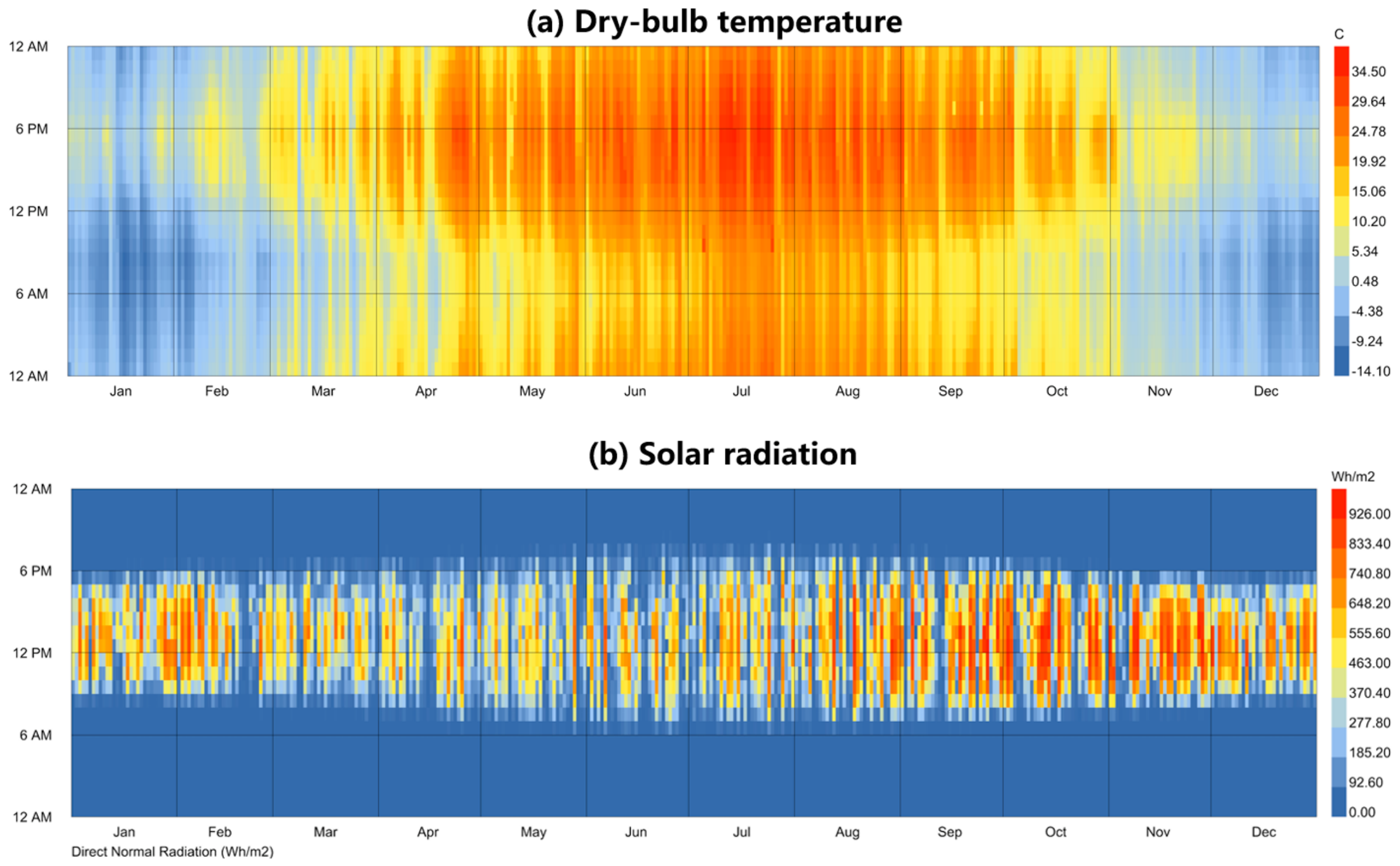
Annual climatic characteristics relevant to daylighting in Lanzhou.
UDI was first calculated at each sensor as the percentage of occupied annual timesteps during which the horizontal illuminance satisfied the inclusive range of 100–2000 lx:
Here, i = 1, …, 180 indexes the sensor locations, and t indexes the hourly timesteps. denotes the horizontal illuminance, in lux, at sensor i during timestep t; denotes the set of occupied annual timesteps; and = || is the total number of occupied hourly timesteps. The indicator function 1(·) equals 1 when its condition is satisfied and 0 otherwise. Both UDI thresholds, 100 lx and 2000 lx, are inclusive.
The resulting UDI values were then spatially averaged across all 180 sensor points:
denotes the arithmetic spatial mean of the sensor-level UDI values across all 180 sensor locations.
DA was calculated using the same spatial averaging procedure:
denotes the percentage of occupied hourly timesteps during which the horizontal illuminance at sensor i is greater than or equal to 300 lx. The threshold is inclusive, and the same occupied-timestep set and denominator defined above are used.
denotes the arithmetic spatial mean of the sensor-level DA values across all 180 sensor locations.
Hourly DGP values for each position–direction sensor were obtained from the results (.dgp) output of HB Imageless Annual Glare. In this study, these values were temporally and spatially aggregated to construct a continuous annual comparative indicator for parametric analysis and multi-objective optimization. For each of the 180 sensor positions, the hourly DGP values were averaged over the 4397 valid sun-up simulation timesteps to obtain a sensor-level annual mean DGP. These sensor-level annual means were then averaged across all 180 sensor positions to obtain the annual spatial-mean DGP indicator used in the subsequent ANOVA, surrogate modelling, NSGA-II optimization, and TOPSIS comparison. All sensor directions were fixed at v = (0, 0, 1), and the same sensor-direction convention was applied consistently across all design alternatives. Accordingly, the annual spatial-mean DGP indicator is interpreted as a standardized measure for comparing the simulated annual glare-related responses of alternative designs under the adopted computational conditions, rather than as a direct representation of occupant-specific glare experience at a particular eye position and viewing direction. For brevity, the annual spatial-mean DGP indicator defined above is hereafter referred to as “DGP” when discussing the response variable used in the statistical analysis, surrogate modelling, and multi-objective optimization. Instantaneous DGP values and sensor-level annual mean DGP values are distinguished explicitly whenever they are discussed. The occurrence of instantaneous glare events, their specific timing, duration, or frequency was not separately recorded, nor was the proportion of time during occupancy periods when DGP exceeded a certain threshold calculated.
Here, denotes the hourly DGP value at sensor i during timestep t, and denotes the total number of valid sun-up hourly timesteps included in the raw (.dgp) output. In this study, = 4397. Unlike UDI and DA, the annual DGP calculation is not restricted to the occupied-hour set ; it uses the valid sun-up timesteps available in the annual glare output.
denotes the arithmetic spatial mean of the sensor-level annual mean DGP values across all 180 sensor locations. It is the annual spatial-mean DGP indicator used as the third optimization objective in this study.
2.4. Statistical Analysis and Surrogate Model Development
For the statistical analysis of the baseline full-factorial design domain, only the 500 complete full-factorial simulation cases were used; neither the 48 independent off-grid validation samples nor the 12 baseline confirmatory samples were included in the ANOVA. UDI, mean DA, and annual spatial-mean DGP were analyzed separately as response variables. WWR, AR, SD, and ORI were all entered as categorical factors in the multifactor ANOVA, with ORI treated explicitly as four discrete orientation categories rather than as a continuous numerical predictor. The ANOVA model included the four main effects and all six two-factor interactions (WWR × AR, WWR × SD, WWR × ORI, AR × SD, AR × ORI, and SD × ORI).
where Y denotes the daylighting performance response variable (UDI, DA, or annual spatial-mean DGP), is the overall mean, represents the main effect of the i-th design factor, represents the two-factor interaction effect between factors i and j, and denotes the residual error term.
No quadratic terms were included in the ANOVA model; the quadratic terms described later belong exclusively to the second-order response-surface surrogate models. The R2 values reported for this analysis refer specifically to the multifactor ANOVA model and are calculated as follows:
where denotes the residual sum of squares of the ANOVA model, and denotes the total sum of squares.
Type II sums of squares were used to quantify the relative contributions of the modeled main effects and two-factor interactions. Because the 500 observations were generated by deterministic simulations, with one outcome for each unique factorial combination, the ANOVA was used primarily as a structured variance-decomposition and effect-ranking procedure within the predefined design domain. The residual term represents response variation not explained by the included main effects and two-factor interactions. Because the factorial combinations were not independently replicated, this residual should not be interpreted as pure experimental or measurement error and may also reflect model lack of fit, including contributions from omitted higher-order interactions. Accordingly, the interpretation emphasizes Type II sums of squares, normalized contribution rates, and modeled response patterns rather than binary statistical-significance classifications. These results are conditional on the selected parameter ranges, factorial design, and ANOVA model structure, rather than universal measures of physical importance or evidence derived from replicated physical experiments.
where is the Type II sum of squares of effect . The residual sum of squares is not included in the denominator of this contribution metric. Therefore, the contributions of the four main effects and six two-factor interactions sum to 100%, apart from minor rounding differences.
The residual term is retained separately and is reported relative to the total sum of squares as
This metric is reported separately from the contribution rates of the main effects and interaction terms because the two metrics use different denominators. The relative contribution of each main effect and two-factor interaction is calculated using the sum of the Type II sums of squares for all included model terms as the denominator, whereas the residual contribution rate is calculated relative to the total sum of squares, .
To develop computationally efficient performance-prediction models for continuous-parameter optimization, second-order response surface models were constructed separately for each of the three performance metrics and each of the four fixed orientation categories, yielding 12 orientation-specific surrogate models. The surrogate models were used as computationally efficient approximations within the sampled and validated design domains, rather than as replacements for high-fidelity simulations outside the regions supported by the available high-fidelity simulation data. Because ORI was handled as a categorical orientation condition, it was not included as a continuous predictor in the response-surface models. Each orientation-specific model used only WWR, AR, and SD as predictors, which were entered in their original engineering units without normalization or standardization. The general form of the model is given as follows:
where denotes the predicted value of the response variable; is the intercept term of the regression model; denotes the number of independent variables; and represent the -th and -th design variables, respectively; is the regression coefficient of the linear term for the -th independent variable; is the regression coefficient of the quadratic term ; and is the regression coefficient of the interaction term between the -th and -th independent variables.
For the surrogate models developed within the baseline design domain, a multi-level validation strategy was adopted to comprehensively assess predictive performance and generalization capability. In addition to evaluating model fit on the training data, five-fold cross-validation and orientation-stratified internal holdout checks were performed as supplementary diagnostics following established model-validation practices [34,35,36]. Cross-validation was used to assess model stability across different data partitions, whereas holdout and independent off-grid validation were reserved for evaluating predictive performance on observations not involved in model fitting. These procedures were used to examine model stability under different data partitions and to reduce the risk of overly optimistic performance estimates based solely on goodness of fit to the training data. During these procedures, validation samples were kept separated from model fitting, parameter estimation, and model-selection procedures to avoid information leakage between training and evaluation datasets. Five-fold cross-validation was used to evaluate the average predictive capability of the models across different subsets of the baseline design domain, whereas the orientation-stratified internal holdout checks provided an additional assessment of predictive performance on samples excluded from model fitting. Meanwhile, the 48 off-grid samples remained fully independent throughout the entire model-development process and were not used for model fitting, parameter estimation, or cross-validation. They were reserved exclusively for evaluating the continuous interpolation capability and in-domain generalization performance of the surrogate models between the regular full-factorial training-grid points. In addition, the 12 TOPSIS confirmatory points selected from the baseline Pareto fronts were not included in surrogate-model training and were subjected to renewed high-fidelity daylight simulations only after completion of the baseline multi-objective optimization. These confirmatory simulations were used to assess the local predictive reliability of the surrogate models within the regions intensively explored by NSGA-II. Through this hierarchical combination of internal validation, independent off-grid validation, and final confirmatory simulations, the stability and reliability of the surrogate models were evaluated from complementary perspectives.
For the geometry-constrained extended design domain, the surrogate models were reconstructed rather than directly reusing those developed for the baseline domain, because both the parameter ranges and sample distribution had changed. Specifically, the 500 baseline full-factorial DOE samples were combined with the 48 additional geometry-constrained extended training samples to form a training dataset comprising 548 samples, thereby expanding the high-fidelity simulation support available for surrogate modeling across the extended parameter space. The same second-order model specification and fitting procedure were applied to each orientation-specific performance model, with WWR, AR, and SD used as predictors and without normalization or standardization of the predictors or response variables. The additional 24 extended-domain samples remained fully independent and were excluded from model fitting, variable selection, and parameter adjustment; they were used exclusively to evaluate the external predictive capability of the extended-domain surrogate models rather than serve as additional optimization samples or decision-making inputs in the newly explored regions of the design space. In parallel, five-fold cross-validation was conducted separately for each building orientation and each performance metric to assess internal model stability and generalization across different training subsets [37,38]. Model performance was evaluated using the coefficient of determination R2, root mean square error (RMSE), and mean absolute error (MAE), thereby characterizing explanatory capability, overall prediction error, and average absolute deviation, respectively [39]. These complementary metrics were jointly used to characterize the predictive accuracy and generalization performance of the extended-domain surrogate models, while recognizing that independent validation alone does not establish predictive reliability at the extreme regions explored by multi-objective optimization. Regarding the reporting scales, MAE, RMSE, and maximum absolute error are expressed in percentage points (pp) for UDI and DA, which are reported on a percentage scale. The corresponding absolute-error measures for the annual spatial-mean DGP indicator are dimensionless. R2 and its confidence intervals are dimensionless, whereas MAPE and signed relative prediction error are expressed as percentages.
2.5. NSGA-II Multi-Objective Optimization and TOPSIS-Based Optimal Solution Selection
NSGA-II was employed to simultaneously maximize mean UDI and mean DA while minimizing the annual spatial-mean DGP indicator. Because ORI is a discrete directional variable, separate surrogate models were developed and independently optimized for the four fixed orientations of 0°, 90°, 180°, and 270°, rather than treating ORI as a continuous genetic variable. For computational consistency, UDI and DA were multiplied by −1 so that all three objectives could be formulated as minimization problems:
where , , and denote mean UDI, mean DA, and annual spatial-mean DGP, respectively, and = [, , ] represents the decision vector for each fixed orientation.
For the extended design domain, the NSGA-II optimization employed a population size of 80, 80 generations, and 10 independent runs with different random seeds. The simulated binary crossover probability was set to 0.90 with a distribution index of = 15, while the polynomial mutation probability was set to 1/3 per decision variable with a distribution index of = 20. The same evolutionary-operator settings were used for the baseline and extended optimizations. All runs were terminated after 80 generations without an early-stopping criterion. This configuration was adopted to balance the search coverage of the multi-objective optimization with computational efficiency, while the repeated independent runs were used to reduce the influence of stochastic initialization, crossover, and mutation on the final optimization results. Each run generated a set of Pareto non-dominated solutions. The Pareto solutions obtained from all 10 runs were subsequently merged, and numerically duplicated or highly overlapping solutions were removed. Non-dominated sorting was then reapplied to the combined candidate set to obtain a unified final Pareto-optimal solution set. A feasible solution A was considered to dominate solution B when ≥ , ≥ , and ≤ , with at least one of these inequalities being strict. Only solutions satisfying the prescribed geometric and surrogate-support constraints were considered eligible for Pareto sorting. The repeated runs and subsequent aggregation were intended to reduce sensitivity to stochastic initialization and improve coverage of the candidate solution set. These procedures assess algorithmic search variability rather than the propagation of surrogate-model prediction errors, which is examined separately through high-fidelity re-simulation of the 20 sampled extended-domain Pareto candidates in Section 3.5. The detailed NSGA-II settings for the baseline and extended design domains are summarized in Table 2.
Table 2.
NSGA-II settings for the baseline full-factorial and extended design domains.
The Pareto solutions obtained using NSGA-II are all non-dominated solutions in the context of multi-objective optimization; however, they do not directly identify a unique design choice. Therefore, TOPSIS was further employed to select representative solutions reflecting different performance preferences. Three weighting scenarios were defined as follows:
, , and represent three architectural design preferences: balanced overall performance, daylight-priority performance, and annual spatial-mean DGP-priority performance, respectively.
For each orientation, TOPSIS was applied to the three performance criteria using min–max normalization. UDI and mean DA were treated as benefit criteria, whereas the annual spatial-mean DGP indicator was treated as a cost criterion. This normalization was applied only to the performance criteria used in TOPSIS. The design variables WWR and AR remained dimensionless ratios, while SD remained expressed in metres. The response-surface surrogate models were fitted using the original engineering scales of WWR, AR, and SD, without normalization or standardization of the predictors. The normalized decision matrix was calculated as follows:
where denotes the original value of the j-th performance criterion for the i-th Pareto candidate solution; represents the normalized criterion value; and denote the minimum and maximum values, respectively, of the j-th criterion among all Pareto candidate solutions for the current orientation; B is the set of benefit criteria, including UDI and DA; and C is the set of cost criteria, including annual spatial-mean DGP.
The normalized decision matrix was then multiplied by the corresponding criterion weights to obtain the weighted normalized decision matrix:
where represents the weighted and normalized indicator value, is the weight corresponding to the j th indicator, and is the normalized indicator value.
The positive and negative ideal solution vectors were determined from the weighted normalized decision matrix as follows:
Here, and denote the positive and negative ideal solution vectors, respectively. Because the cost-type DGP criterion has been reversed during the normalization in Equation (16), larger normalized values indicate better performance for all three criteria. Accordingly, comprises the maximum weighted normalized value for each criterion, whereas comprises the minimum value for each criterion.
The Euclidean distances of each candidate solution from the positive and negative ideal solutions were calculated using the weighted normalized decision matrix as follows:
where and respectively represent the Euclidean distances from the i-th candidate solution to the positive and negative ideal solutions, while and respectively denote the components of the two ideal solutions in the j-th criterion.
For each building orientation and each weighting scenario, the solution with the largest value was selected as the representative optimal solution. The relative closeness coefficient was calculated as follows:
where denotes the relative closeness of the -th solution to the ideal solution; represents the weighted Euclidean distance between the -th solution and the positive ideal solution; and represents the weighted Euclidean distance between the -th solution and the negative ideal solution.
3. Results
3.1. Effects of Design Parameters on Daylighting Performance
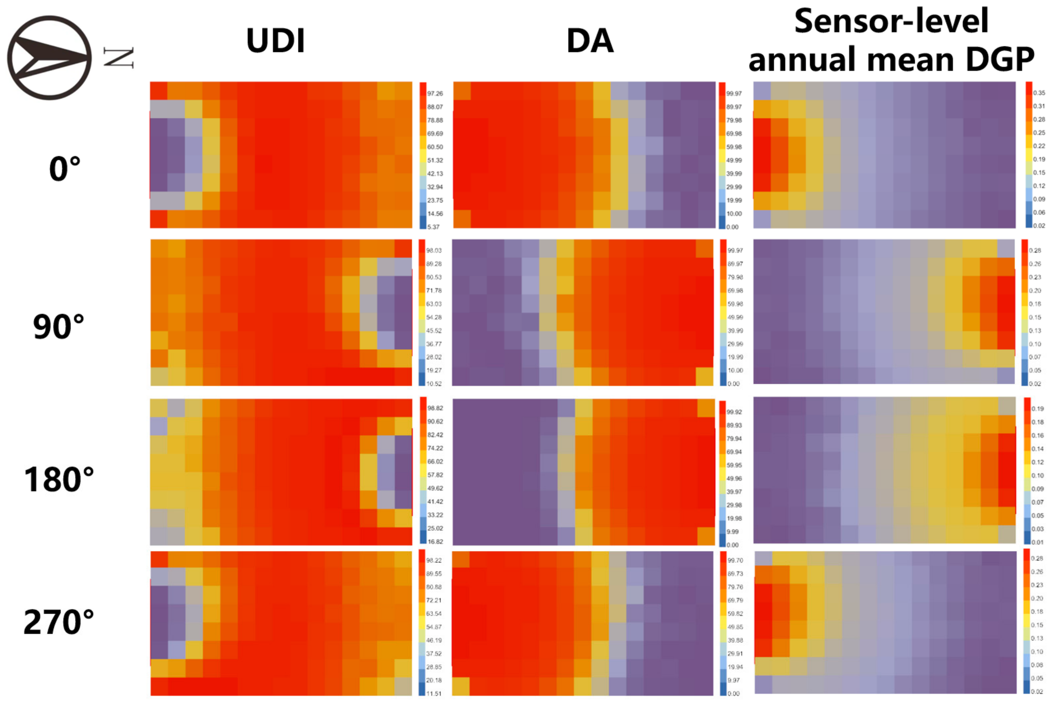
To provide a spatial interpretation of the simulated daylighting metrics, Figure 6 presents the spatial distributions of sensor-level UDI, point-based DA, and sensor-level annual mean DGP for a representative baseline configuration (WWR = 0.40, AR = 0.80, SD = 0) under the four orientations. The results illustrate orientation-dependent differences in daylight availability and in the spatial distribution of sensor-level annual mean DGP values, particularly in regions adjacent to the facade. The orientation convention follows the Grasshopper model definition, with 0° = South, 90° = East, 180° = North, and 270° = West, using counterclockwise rotation referenced to geographic south.
Figure 6.
Spatial distributions of sensor-level UDI, point-based DA, and sensor-level annual mean DGP under the four orientations for a representative baseline configuration (WWR = 0.40, AR = 0.80, SD = 0 m).
Based on the 500 complete full-factorial simulation cases (Figure 7), multifactor analysis of variance (ANOVA) was conducted to quantify the effects of WWR, AR, SD, and ORI, as well as their two-factor interactions, on daylighting performance. In the original dataset, UDI ranged from 66.230% to 82.635%, with a mean value of 75.667%; DA ranged from 33.665% to 66.382%, with a mean of 50.537%; and annual spatial-mean DGP ranged from 0.1010 to 0.2496, with a mean of 0.1658. These results indicate that, under identical office-space geometry and material boundary conditions, variations in fenestration configuration, external shading depth, and building orientation alone can produce substantial differences in annual daylighting performance.
Figure 7.
Parameter and response distribution matrix for the baseline full-factorial dataset.
The relative contribution of each modeled main effect and two-factor interaction was quantified as the proportion of its Type II sum of squares to the sum of the Type II sums of squares for all included main effects and two-factor interactions. Type II sums of squares were adopted because the analysis focused on estimating the contribution of each main effect and interaction term under the balanced factorial design structure, while avoiding the dependence on arbitrary sequential entry order associated with Type I sums of squares. Because this measure is additive across all main effects and two-factor interaction terms, the unrounded contributions sum to 100%; the displayed percentages may differ slightly from 100% because of rounding. This provides a consistent basis for comparing the relative contribution of different modeled terms within the investigated simulation-based design domain. These contribution values should therefore be interpreted as conditional variance decomposition results associated with the selected parameter ranges, experimental design, and model structure, rather than as universal measures of physical importance across all building contexts (Figure 8). Within the analyzed simulation-based design domain, the corresponding multifactor ANOVA models yielded R2 values of 0.9967, 0.9996, and 0.9991 for UDI, mean DA, and annual spatial-mean DGP, respectively. These R2 values refer to the fitted ANOVA models and indicate that the included main effects and two-factor interactions explain most of the total response variation within the predefined parameter ranges (Figure 9).
Figure 8.
Relative contributions of main effects and two-way interactions from the multifactor ANOVA.
Figure 9.
Main effects of WWR, AR, SD, and ORI on UDI, DA, and annual spatial-mean DGP.
For UDI, WWR exhibited the largest relative contribution within the investigated design domain, accounting for 69.48% of the model-explained sum of squares. AR had the second-largest relative contribution, accounting for 9.71%, whereas ORI and SD accounted for 3.14% and 0.88%, respectively. Notably, the combined contribution of two-factor interactions to UDI reached 16.78%, substantially higher than those observed for DA and DGP. Among these interactions, WWR × ORI showed the largest contribution, at 11.17%, followed by SD × ORI and WWR × SD, which contributed 2.09% and 2.07%, respectively. These results indicate that, within the investigated parameter ranges, UDI is influenced not only by window area itself, but also by the extent to which the effect of window area varies with building orientation. Therefore, discussing WWR, shading, and orientation as completely independent design factors would overlook a considerable proportion of the parameter-coupling effects affecting UDI (Figure 10).
Figure 10.
Selected two-way interaction effects identified from the multifactor ANOVA.
For DA, the main effects accounted for 99.49% of the total Type II sums of squares attributed to the modeled terms, whereas two-factor interactions contributed 0.51%. WWR showed the largest relative contribution, at 58.26%, followed by ORI at 28.73% and SD at 12.37%, while AR contributed only 0.13%. The largest two-factor interaction, WWR × AR, contributed 0.257%. These percentages describe the relative contributions of the modeled terms within the specified design domain. Given the deterministic and unreplicated nature of the simulation dataset, the interaction terms are interpreted according to their relative contribution magnitudes rather than classified solely by statistical-significance thresholds. Within the investigated parameter ranges, the modeled DA variation was dominated by WWR, ORI, and SD, whereas the contribution of AR was comparatively small.
The contribution structure for DGP differed markedly from those of UDI and DA. ORI showed the largest relative contribution within the investigated design domain, accounting for 56.20% of the model-explained sum of squares, while WWR, SD, and AR contributed 26.95%, 13.55%, and 1.53%, respectively. Two-factor interactions collectively accounted for 1.77%, with SD × ORI showing the largest contribution at 0.916%, followed by WWR × ORI and AR × SD at 0.450% and 0.328%, respectively. These results indicate that the annual spatial-mean DGP indicator shows a pronounced variation with building orientation, while window area and external shading depth also represent important geometric factors associated with its variation within the investigated design domain (Table 3).
Table 3.
Multifactor ANOVA contribution summary.
It should be noted that the ANOVA contribution values represent conditional variance decomposition within the predefined simulation design domain [40,41,42]. Therefore, these values describe the relative contribution of each factor under the selected parameter ranges and experimental structure, rather than universal measures of design importance beyond the investigated conditions. Further examination of the marginal means at different parameter levels provides a clearer understanding of the direction of each factor’s influence. As WWR increased from 0.30 to 0.50, the mean UDI rose steadily from 70.62% to 78.75%, corresponding to an increase of 8.13 percentage points, while DA increased from 42.85% to 57.52%, i.e., 14.67 percentage points. Over the same range, DGP increased from 0.1428 to 0.1864. These results indicate that enlarging the window area can substantially enhance daylight utilization, but is accompanied by an increase in the annual spatial-mean DGP indicator. WWR therefore represents an important design variable associated with the trade-offs among the three daylighting objectives within the investigated simulation domain.
AR exhibited different responses across the three performance metrics. As AR increased from 0.40 to 1.20, UDI increased from 73.86% to 76.96%, corresponding to an overall increase of approximately 3.10 percentage points. By contrast, DA decreased only slightly from 50.85% to 50.20%, indicating a relatively limited effect. The annual spatial-mean DGP indicator decreased progressively from 0.1714 to 0.1613. These results suggest that, under a given WWR, adjusting the geometric proportions of the window opening can moderately improve UDI and reduce the annual spatial-mean DGP indicator, whereas its association with DA is substantially weaker than that of WWR, ORI, and SD. Increasing SD produced a typical daylight–annual spatial-mean DGP trade-off. As SD increased from 0 to 1.20 m, DA decreased continuously from 54.18% to 47.47%, while the annual spatial-mean DGP indicator declined from 0.1825 to 0.1518. In contrast, UDI exhibited a non-monotonic response to increasing SD. It initially increased from 75.06%, reached approximately 75.98% at SD = 0.90 m, and then declined slightly to 75.92% at SD = 1.20 m. This pattern indicates that moderate external shading can reduce the adverse effects of excessive daylight on UDI by shifting some overlit conditions back into the useful illuminance range. However, when shading becomes excessively deep, the associated loss of daylight begins to offset this benefit.
The categorical ORI factor also produced pronounced differences in daylighting performance. At 0°, the mean DA was the highest, reaching 54.71%, but the corresponding annual spatial-mean DGP value was also the highest, at 0.1900. In contrast, the 180° orientation exhibited the lowest DA, at 44.71%, together with the lowest annual spatial-mean DGP value, at only 0.1298. The results for 90° and 270° were very similar, with DA values of 51.34% and 51.39%, respectively, and DGP values of approximately 0.1716 for both orientations. UDI was generally less sensitive to orientation than DA and the annual spatial-mean DGP indicator, reaching 76.12% and 76.31% at 90° and 270°, respectively, compared with 74.69% at 0°.
3.2. Performance of the Surrogate Models
Second-order response surface models were developed separately for UDI, DA, and DGP under each of the four orientation conditions, resulting in a total of 12 independent surrogate models. To avoid assessing model performance solely on the basis of goodness of fit to the training data, this study employed multiple validation procedures, including five-fold cross-validation, internal holdout validation, and independent validation using 48 off-grid samples (Figure 11). Performance metrics for the training, cross-validation, internal holdout, and independent validation stages were recorded separately, allowing the models’ fitting capability to be distinguished from their actual in-domain generalization performance.
Figure 11.
Prediction performance for the 48 independent off-grid validation samples.
For the training data, the R2 values of the UDI models ranged from 0.9907 to 0.9965, while those of the DA models ranged from 0.9989 to 0.9992 and those of the DGP models from 0.9975 to 0.9981. The five-fold cross-validation results were highly consistent with the training results. Specifically, the CV-R2 values ranged from 0.9887 to 0.9953 for UDI, from 0.9986 to 0.9990 for DA, and from 0.9977 to 0.9984 for DGP. No evident pattern was observed in which the training accuracy substantially exceeded the cross-validation accuracy, indicating that the models maintained stable predictive performance across different data subsets.
More importantly, the 48 fully independent off-grid samples also demonstrated high predictive accuracy (Table 4). When the four orientations were pooled, the independent-validation R2 for UDI was 0.9936, with an RMSE of 0.237 percentage points and an MAE of 0.197 percentage points. For DA, the corresponding R2, RMSE, and MAE were 0.9990, 0.180 percentage points, and 0.144 percentage points, respectively. For the annual spatial-mean DGP indicator, the independent-validation R2 reached 0.9994, with an RMSE of 0.000630 and an MAE of 0.000519; both DGP error measures are dimensionless. A bootstrap analysis based on 2000 orientation-stratified resampling iterations was used to estimate the reported 95% confidence intervals. When the results were examined separately by orientation, the independent-validation R2 values ranged from 0.9878 to 0.9968 for UDI, from 0.9978 to 0.9987 for DA, and from 0.9968 to 0.9989 for DGP. Compared with the DA and DGP models, the UDI models exhibited slightly larger prediction errors, but still demonstrated strong continuous-parameter interpolation capability. Considering that the 48 validation samples were completely excluded from model fitting and were deliberately positioned between the original 5 × 5 × 5 regular parameter-grid points, these results indicate that the second-order response surface models can robustly characterize the continuous relationships between WWR, AR, and SD and the three daylighting performance metrics within the baseline design domain [40,41,42]. Therefore, the surrogate models were considered suitable for interpolation and preliminary optimization within the validated baseline parameter domain; their reliability in specific high-performing regions was subsequently examined through high-fidelity re-simulation of the 12 TOPSIS-selected solutions, while their applicability remained limited to the design space supported by the available simulation samples.
Table 4.
Independent off-grid validation of the quadratic surrogate models.
3.3. Optimization Results Within the Baseline Full-Factorial Design Domain
After confirming the surrogate models’ predictive performance within the validated baseline domain, NSGA-II optimization was performed independently for each fixed building orientation. The final implementation used a population size of 80, 80 generations, and 10 independent runs per orientation. Simulated binary crossover was applied with a crossover probability of 0.90 and distribution index = 15, while polynomial mutation was applied independently to each decision variable with a probability of 1/3 and distribution index = 20. For reproducibility, run-specific random seeds were generated as , where denotes the run index from 1 to 10. Under the minimization formulation (−UDI, −DA, DGP), solution A was defined to dominate solution B when it was no worse in all three objectives and strictly better in at least one objective. Pareto fronts from the 10 runs were merged, numerical duplicates were removed using a normalized decision-space tolerance of , and non-dominated sorting was reapplied to the merged candidate set. All runs were completed for 80 generations; convergence was assessed retrospectively using relative changes in the three ideal objective values and normalized Hausdorff movement of the Pareto front, with convergence flagged when all criteria remained below predefined thresholds for 10 consecutive generation transitions, rather than serving as an early-stopping criterion.
Within the baseline full-factorial design domain, continuous three-objective Pareto fronts were obtained for all four orientations (Figure 12, Figure 13, Figure 14 and Figure 15). After merging the results from the 10 independent runs and removing duplicate solutions, 487, 500, 588, and 499 non-dominated solutions were retained for the 0°, 90°, 180°, and 270° orientations, respectively. The final Pareto solutions and their predicted objective values characterize the trade-offs among UDI, DA, and the annual spatial-mean DGP indicator. These solutions clearly revealed the trade-offs among UDI, DA, and the annual spatial-mean DGP indicator. Higher DA generally required larger WWR and shallower external shading, whereas lower annual spatial-mean DGP tended to favor smaller WWR and greater SD. By contrast, regions with high UDI reflected a compromise among relatively large WWR, high AR, and some degree of external shading, rather than a single dominant geometric strategy.
Figure 12.
Pareto fronts within the baseline full-factorial design domain for the 0° orientation.
Figure 13.
Pareto fronts within the baseline full-factorial design domain for the 90° orientation.
Figure 14.
Pareto fronts within the baseline full-factorial design domain for the 180° orientation.
Figure 15.
Pareto fronts within the baseline full-factorial design domain for the 270° orientation.
With respect to the individual objective extrema along the Pareto fronts, the maximum UDI, maximum DA, and minimum annual spatial-mean DGP values at 0° were 79.38%, 66.55%, and approximately 0.1450, respectively. The corresponding values at 90° were 81.52%, 62.19%, and 0.1329; at 180°, 82.92%, 54.51%, and 0.1020; and at 270°, 81.53%, 62.19%, and 0.1333. It should be emphasized that these three extrema correspond to different Pareto-optimal solutions and therefore cannot be achieved simultaneously within a single design. This illustrates that the three modeled objectives cannot generally be optimized simultaneously within a single design in the investigated domain, supporting the use of multi-objective analysis to characterize the trade-offs among them. These DGP extrema should be interpreted as extrema of the annual spatial-mean DGP indicator used here, not as evidence that short-duration or occupant-specific glare events were eliminated. The reported DGP values are used for comparative optimization within this metric definition and are not interpreted against conventional instantaneous DGP thresholds.
The top 10% of Pareto solutions ranked under the Equal-TOPSIS scenario exhibited pronounced boundary concentration in WWR and AR across all four orientations. The overall 10th–90th percentile range was 0.464–0.500 for WWR and 1.116–1.200 for AR, whereas SD showed substantially greater dispersion (Figure 16). This pattern indicates that the high-ranking baseline-domain solutions were concentrated near the predefined boundaries. However, such boundary concentration does not demonstrate that WWR = 0.50 or AR = 1.20 represents a physically optimal value; rather, it suggests that the predefined search bounds may be constraining the exploration of potentially higher-performing regions. This observation was therefore treated as a boundary-sensitivity indication rather than evidence of a global optimum. Accordingly, the subsequent extended-domain analysis was designed to test whether the observed boundary concentration persisted after the original rectangular limits were relaxed, rather than to assume that a newly introduced boundary represented a physically optimal value.
Figure 16.
Orientation-specific parameter ranges among the top−ranked baseline-domain TOPSIS candidates.
3.4. Optimization Results Within the Geometry-Constrained Extended Design Domain
Because the top-ranked Pareto solutions in the baseline full-factorial design domain exhibited pronounced concentration at the WWR and AR boundaries, a geometry-constrained extended design domain was introduced to test the sensitivity of the optimization results to the original parameter boundaries. This investigation employed explicit window-opening geometric constraints and additional high-fidelity simulations. The extended domain was defined as a geometry-constrained simulation domain rather than a complete architectural feasibility domain. Structural self-weight, wind loads, facade integration, view obstruction, construction, and maintenance requirements were not explicitly modeled. The extended surrogate models were trained using a combined dataset consisting of the 500 baseline DOE samples and 48 additional geometrically feasible training samples, resulting in a total of 548 training cases. Meanwhile, 24 samples from the extended design domain were retained as a fully independent validation set. These 24 independent samples were used to assess general predictive performance across the extended domain, but they do not by themselves establish high-fidelity accuracy at every Pareto extreme or boundary-adjacent solution. Unlike the baseline parameter domain, the extended domain no longer restricted WWR to 0.30–0.50 or AR to 0.40–1.20. Instead, the NSGA-II search was confined to the WWR–AR envelope covered by the actual extended training data, while dynamically enforcing the 0.30 m window-opening edge-margin constraint. The allowable range of SD was also extended to 0–3.00 m. This strategy relaxed the original fixed rectangular parameter bounds while preventing unrestricted surrogate-model extrapolation into regions lacking support from actual Honeybee simulations. Therefore, the extended-domain optimization should be interpreted as a boundary-sensitivity investigation within the simulation-supported design region, rather than as evidence of a global optimum or a universally optimal architectural solution.
The extended surrogate models showed generally good predictive performance on the 24 fully independent validation samples, although the prediction accuracy varied across indicators and orientations (Figure 17). The pooled R2 values for UDI, DA, and the annual spatial-mean DGP indicator were 0.9710, 0.9919, and 0.9977, respectively, with corresponding RMSE values of 1.370 percentage points, 0.929 percentage points, and 0.001490. The corresponding MAE values were 1.078 percentage points, 0.732 percentage points, and 0.001128. Compared with the surrogate models developed for the baseline design domain, the prediction error for UDI increased after domain expansion, indicating that the second-order response-surface approximation was less accurate over the expanded domain. In particular, the independent-validation R2 for UDI at 0° was 0.9289, the lowest among all orientation-specific models. Therefore, predictions near the parameter-space boundaries for this orientation should be interpreted with comparatively greater caution.
Figure 17.
Prediction performance for the 24 independent extended-domain validation samples.
To assess local surrogate reliability in the extreme regions explored by the optimization, one maximum-UDI, one maximum-DA, and one minimum-annual-spatial-mean-DGP solution for each orientation were re-simulated using the original Honeybee simulation workflow, giving 12 optimization-targeted confirmatory cases in total (Table 5). After optimization with a population size of 80, 80 generations, and 10 independent runs, the extended design domains for 0°, 90°, 180°, and 270° yielded 558, 537, 531, and 511 merged non-dominated solutions, respectively. Compared with the individual extrema of the three objectives in the baseline Pareto sets, the surrogate-based extended-domain results indicated larger predicted attainable ranges for all three daylighting metrics.
Table 5.
Comparison of single-objective Pareto extrema between the baseline and geometry-constrained extended design domains.
The surrogate-based Pareto results within the extended design domain revealed three differentiated extreme-objective patterns. First, at the maximum predicted UDI for each orientation, the solutions exhibited relatively large WWR values, external shading depths close to 3.0 m, and window heights reaching the geometric upper limit of 2.40 m. The corresponding WWR values for 0°, 90°, 180°, and 270° are approximately 0.587, 0.598, 0.632, and 0.594, respectively, while the corresponding AR values are approximately 0.779, 0.764, 0.723, and 0.770. Within the investigated extended domain, the maximum-predicted-UDI solutions did not continue to increase AR beyond the baseline upper bound of 1.20. Instead, they tended to combine larger overall window area, fuller use of the available window height, and deeper external shading.
Second, the maximum-DA solutions identified for the four orientations in the extended domain exhibited similar parameter patterns, with WWR values of approximately 0.662, AR values of approximately 0.690, SD values close to 0 m, and window heights reaching 2.40 m. Within the investigated domain, these solutions were associated with relatively large unobstructed window openings and higher annual spatial-mean DGP values. They should therefore be interpreted as high-DA solutions involving a trade-off with the annual spatial-mean DGP objective, rather than as uniformly balanced solutions across all three objectives.
By contrast, the solutions corresponding to the minimum predicted annual spatial-mean DGP for all four orientations tended toward WWR values of approximately 0.186, AR values of approximately 0.355, and SD values of approximately 3.0 m. Under these conditions, the predicted annual spatial-mean DGP decreased to approximately 0.069–0.079, but both UDI and DA decreased substantially. This further demonstrates that extending the parameter ranges does not eliminate the conflicts among the performance objectives; rather, it broadens the design space within which different performance preferences can be accommodated.
In addition, a certain degree of boundary concentration remains evident along the extended Pareto fronts (Figure 18). The proportions of Pareto-optimal solutions located near the SD boundaries of 0 or 3.0 m are 46.6%, 68.9%, 65.5%, and 68.9% for the 0°, 90°, 180°, and 270° orientations, respectively. The proportions of solutions in which the window height reaches the geometric limit imposed by the 0.30 m upper and lower edge margins are 29.0%, 25.0%, 15.1%, and 23.3%, respectively. Meanwhile, approximately 11.9–22.8% of the solutions lie near the edge of the extended training envelope for WWR, while the corresponding proportion for AR is approximately 11.3–22.0%. These patterns indicate that the extended-domain Pareto solutions are influenced by the adopted SD limits, geometric window-height constraint, and training-envelope boundaries. Such boundary concentration may reflect directional performance-response trends within the investigated region, the influence of the remaining constraints, or both. Accordingly, the observed improvements are interpreted as conditional candidate performance gains within the geometry-constrained, simulation-supported domain, rather than as proof of a boundary-independent global optimum.
Figure 18.
Boundary concentration of Pareto solutions in the baseline and geometry-constrained extended design domains.
3.5. High-Fidelity Confirmation of Sampled Pareto Candidates
To further examine surrogate-model reliability beyond the single-objective extrema, 20 additional Pareto candidates were selected from the extended-domain solution sets, with five candidates evaluated for each facade orientation. The candidates were selected from five clusters in the normalized objective space for each orientation, with the candidate closest to each cluster centroid retained. Each candidate was then re-simulated using the original Grasshopper–Honeybee workflow (Table 6).
Table 6.
Summary of high-fidelity confirmation results for 20 extended-domain Pareto candidates.
Across the 20 sampled candidates, the surrogate predictions preserved 37 of 40 within-orientation pairwise rankings for UDI, corresponding to 92.5%, and all 40 rankings for both mean DA and the annual spatial-mean DGP indicator, corresponding to 100% for each metric. Thus, three UDI pairwise orderings differed between the surrogate predictions and high-fidelity simulation results. The Pareto-dominance classifications were unchanged across all 40 within-orientation candidate pairs. However, no pair was classified as dominating another under either the surrogate predictions or the high-fidelity simulation results. Accordingly, this check indicates that no dominance-classification reversals were observed among the sampled pairs, but it does not independently establish the dominance structure of the entire Pareto front. Together with the prediction-error metrics, these results provide candidate-level evidence that the relative rankings of the sampled trade-off solutions were generally preserved under high-fidelity simulation. Because the candidates were selected from five clusters in the normalized objective space rather than exhaustively re-simulated across the continuous solution set, this analysis does not establish the exact locations of all Pareto extrema or the stability of the entire Pareto front under surrogate-model error or further expansion of the search domain.
3.6. TOPSIS-Selected Representative Solutions and High-Fidelity Validation
To further identify representative solutions from the Pareto fronts of the baseline design domain for architectural decision-making, TOPSIS was applied under three weighting scenarios: Equal, Daylight-Balanced, and Annual-DGP-Priority. Annual-DGP-Priority The corresponding weights were set to (1/3, 1/3, 1/3), (0.45, 0.45, 0.10), and (0.20, 0.20, 0.60), respectively.
Under the Equal scenario, the selected compromise solutions for all four orientations were located close to the upper bounds of the original WWR, AR, and SD ranges. For 0°, the selected solution was WWR = 0.500, AR = 1.200, and SD = 1.200 m, with predicted values of UDI = 79.38%, DA = 59.58%, and annual spatial-mean DGP = 0.1934. For 90°, the corresponding parameter combination was WWR = 0.500, AR = 1.200, and SD = 1.200 m, yielding UDI = 81.52%, DA = 55.85%, and annual spatial-mean DGP = 0.1761. For 180°, the selected solution was WWR = 0.499, AR = 1.195, and SD = 1.177 m, with UDI = 82.14%, DA = 48.66%, and annual spatial-mean DGP = 0.1359. For 270°, the corresponding values were WWR = 0.496, AR = 1.200, and SD = 1.200 m, with predicted UDI = 81.49%, DA = 55.61%, and annual spatial-mean DGP = 0.1755.
As the decision weights changed, the selected representative solutions shifted markedly (Table 7). Under the Daylight-Balanced scenario, WWR and AR remained at relatively high levels, whereas SD decreased substantially. The corresponding SD values for 0°, 90°, 180°, and 270° were approximately 0.787, 0.394, 0, and 0.384 m, respectively, resulting in higher DA. By contrast, under the Annual-DGP-Priority scenario, WWR decreased markedly to approximately 0.327–0.336, while SD increased to approximately 1.133–1.198 m. Within these selected solutions, lower annual spatial-mean DGP values were associated with smaller transparent opening areas and greater external shading depth.
Table 7.
Representative TOPSIS solutions within the baseline full-factorial design domain.
The 12 representative solutions were subsequently reintroduced into the original Grasshopper–Honeybee model for high-fidelity confirmatory daylight simulations, and the resulting performance values showed small differences from the corresponding surrogate-model predictions [43,44] (Figure 19). For UDI, the confirmatory validation yielded an R2 of 0.9983, an RMSE of 0.160 percentage points, and an MAE of 0.126 percentage points. For DA, the corresponding values were R2 = 0.9993, RMSE = 0.2022 percentage points, and MAE = 0.1583 percentage points. For the annual spatial-mean DGP indicator, the R2, RMSE, and MAE were 0.9989, 0.0009, and 0.008, respectively. The mean absolute percentage errors (MAPE) for UDI, DA, and the annual spatial-mean DGP indicator were approximately 0.16%, 0.31%, and 0.498%, respectively.
Figure 19.
Relative prediction errors of the 12 confirmatory simulations.
For the individual solutions, the maximum absolute relative errors were approximately 0.39% for UDI, 0.85% for DA, and 0.88% for the annual spatial-mean DGP indicator, with no substantial prediction deviations observed across any of the 12 cases (Table 8).
Table 8.
Confirmatory simulation accuracy.
These results support the predictive accuracy of the 12 TOPSIS-selected representative solutions within the baseline design domain. Because these cases were selected to represent specific decision preferences, they provide a targeted assessment of those representative designs rather than a validation of the entire Pareto front. The additional high-fidelity confirmation of 20 sampled extended-domain Pareto candidates is reported separately in Section 3.5 and examines prediction errors, relative rankings, and pairwise dominance classifications in selected multi-objective trade-off regions. Together, these evaluations provide complementary evidence for the surrogate-assisted optimization framework while keeping the scope of the validation explicit.
The signed relative prediction error for case i was calculated as , where denotes the Honeybee-simulated value and denotes the surrogate-model prediction. Under this convention, positive values indicate surrogate-model underprediction, whereas negative values indicate overprediction.
4. Discussion
4.1. Interpretation of Fenestration Parameter Effects Within the Investigated Domain
Within the investigated simulation domain, annual daylighting performance varied systematically with window area, fenestration geometry, external shading, and building orientation, although the magnitude and direction of the response differed considerably across performance metrics. WWR accounted for the largest share of model-explained variance in UDI and DA, whereas ORI accounted for the largest share for the annual spatial-mean DGP indicator within the specified ANOVA design. In addition, the relatively large contribution of the WWR × ORI interaction to UDI indicates that the modeled response of UDI to WWR varied across the four orientations. This implies that even when the same WWR is adopted, facades with different orientations may exhibit markedly different annual daylighting responses because of differences in the timing and intensity of incident solar radiation. Window parameters should therefore be evaluated jointly with facade orientation rather than determined independently of it.
The relatively large contribution of WWR is consistent with the direct role of transparent opening area in admitting daylight into the interior [45,46,47,48]. Increasing WWR generally improved DA and was associated with greater daylight availability in deeper parts of the room; however, larger transparent openings may also increase the annual spatial-mean DGP response under certain solar and orientation conditions. Within the investigated domain, these results indicate a trade-off between daylight utilization and the annual spatial-mean DGP response captured by the adopted indicator. In other words, simply increasing the transparent opening area does not guarantee simultaneous improvement in all daylighting metrics, and an appropriate WWR should be determined in conjunction with shading conditions and building orientation.
Although AR accounted for a relatively small share of the variation in DA, changes in AR were associated with noticeable changes in UDI and the annual spatial-mean DGP indicator within the investigated range. This pattern may be associated with changes in the horizontal-to-vertical proportions and vertical placement of the window opening, which can alter daylight penetration and the spatial distribution of the sensor-level annual DGP response under the adopted imageless calculation workflow. SD, by contrast, showed a dual response in the present simulations. Increasing shading depth was associated with reductions in both the annual spatial-mean DGP value and DA, while moderate shading could also reduce excessive illuminance above the upper UDI threshold, allowing some previously overlit periods to return to the useful illuminance range. Within the investigated range, external shading was associated not only with lower annual spatial-mean DGP values but also, at moderate depths, with improved UDI through changes in the annual distribution of indoor illuminance.
The large ANOVA contribution of ORI to the annual spatial-mean DGP indicator, together with the orientation-specific differences in the results, indicates that this response was more orientation-dependent than UDI and DA within the investigated domain, suggesting that identical window-shading configurations may not be directly transferable across different facades. At the same time, the larger interaction contributions associated with UDI and the larger validation errors observed in the extended domain suggest that UDI was less well approximated by the second-order response surface and may exhibit more complex response behavior in the expanded domain. These findings further imply that, in parametric daylighting optimization, single-factor sensitivity analysis alone may be insufficient to capture the actual design relationships, and particular attention should be paid to the combined effects of window area, external shading, and building orientation.
4.2. Trade-Offs Among UDI, DA, and the Annual Spatial-Mean DGP Indicator
Within the baseline design domain, the higher-DA Pareto solutions tended to occur at larger WWR values and shallower external shading, whereas the lower annual spatial-mean DGP solutions tended to occur at smaller WWR values and deeper shading. These patterns describe the solutions identified under the specified objectives and parameter ranges; they should be interpreted as domain-specific associations rather than universal or strictly causal design rules. The TOPSIS-selected solutions further illustrate how changing the decision weights changes the preferred compromise among the modeled metrics.
UDI introduces additional complexity because it excludes both insufficient and excessive illuminance. Moderate shading may reduce DA while bringing some overlit periods above 2000 lx back into the useful illuminance range. In the present simulations, high-UDI solutions were associated with coordinated combinations of WWR, AR, and SD rather than with increasing window area alone. In the extended domain, the high-UDI solutions were concentrated around relatively large WWR, moderate AR, and deeper shading. Because these solutions also occurred near the SD, geometric, or training-envelope boundaries, this pattern should be interpreted as a boundary-sensitive tendency within the current simulation-supported domain rather than as evidence of a stable physical optimum.
To complement pointwise prediction-error metrics, the 20-candidate high-fidelity assessment in Section 3.5 examined pairwise ranking agreement and Pareto dominance consistency across sampled trade-off regions. The results support the relative ordering of the sampled candidates under the current constraints, while not establishing the exact locations of all Pareto extrema or the stability of the entire continuous Pareto front under surrogate-model error.
Although shading depths close to 3.0 m are geometrically feasible under the constraints adopted in this study, they should not be interpreted as directly constructible facade solutions. Such deep external shading devices may impose additional structural and self-weight requirements, increase wind-load demands, complicate facade integration and detailing, obstruct outdoor views, and increase construction and maintenance requirements. These factors were not explicitly modeled in the present simulation framework. Therefore, the extended-domain results should be interpreted as daylight-performance trends within a simulation-supported geometric domain rather than as direct prescriptions for architectural implementation.
In this study, the role of TOPSIS is not to identify a single universally “best” window configuration, but to map different performance preferences onto representative solutions along the Pareto front. The Equal, Daylight-Balanced, and Annual-DGP-Priority scenarios respectively represent balanced overall performance, daylight-priority performance, and lower annual spatial-mean DGP-priority performance. In practical architectural design, the decision weights can be adjusted according to space function, occupant visual-comfort requirements, and other performance objectives, allowing different solutions to be selected from the same Pareto-optimal set. The contribution of TOPSIS in this study is to illustrate how the three specified weighting scenarios select different representative window–shading configurations from the Pareto sets generated within the investigated design domain. The selected configurations are preference-dependent examples rather than universally optimal parameter combinations.
4.3. Comparison Between the Baseline and Extended Design Domains
The pronounced boundary concentration of WWR and AR observed in the baseline full-factorial design domain should be interpreted in relation to the structure of the initial DOE. Because WWR and AR jointly determine the window-opening area, height, and width, relatively conservative rectangular bounds were adopted at the baseline stage to ensure both the geometric feasibility of all full-factorial combinations and the statistical balance of the experiment. Therefore, the repeated convergence of high-ranking solutions toward WWR = 0.50 and AR = 1.20 more likely indicates that the optimization has reached the predefined search boundaries, rather than demonstrating that these values represent universally applicable physical optima. In this context, boundary concentration should be regarded primarily as a diagnostic signal indicating the need to further examine the adequacy of the design domain.
To investigate this boundary effect, additional Honeybee simulations were introduced to expand the coverage of the training samples, while the extended search space was jointly constrained by the 0.30 m window-edge margin and the actual coverage of the training data. This strategy was adopted to prevent the surrogate models from extrapolating directly into regions lacking high-fidelity simulation support. However, remaining within the training-data envelope does not guarantee uniform local prediction accuracy, particularly near its boundaries where sample density may be lower. Therefore, the extended-domain optimization results should be interpreted only within the simulation-supported region assessed by the independent validation samples, and should not be considered as evidence of a complete global optimum. After extension, the high-UDI solutions shifted from the baseline-domain pattern of “large WWR + high AR” toward combinations characterized by WWR values of approximately 0.59–0.63, AR values of approximately 0.72–0.78, and deep external shading close to 3.0 m. This migration is consistent with a compensatory association among window area, window proportions, and shading depth within the investigated design domain. In other words, once the window-opening geometric constraints are explicitly incorporated, the high-UDI solutions did not simply continue toward simultaneously larger window area and window aspect ratio, but instead reflected a reconfiguration of multiple interacting design parameters.
The observed parameter migration indicates that the selected design-domain bounds can influence the parameter patterns identified by optimization in this study (Figure 20). A regular full-factorial design is advantageous for statistical analysis and comparison of factor effects, but its fixed rectangular bounds do not necessarily cover all potentially high-performing regions associated with geometrically coupled variables. By contrast, the geometry-constrained extended domain enables these regions to be explored further while maintaining the predefined geometric feasibility constraints. Distinguishing between a statistical design domain and a geometry-constrained extended design domain can therefore help avoid misinterpreting artificially imposed parameter bounds as true performance-optimal boundaries [49,50].
Figure 20.
Parameter migration from the baseline full-factorial to the geometry−constrained extended design domain.
Nevertheless, the extended domain represents a geometry-constrained, simulation-supported search region rather than a complete global feasible domain. The observed concentration near the SD limits, geometric window-height constraint, and training-envelope boundaries indicates that the identified extrema remain conditional on the adopted search settings. Such concentration is compatible with directional performance-response trends within the investigated region and with sensitivity to the remaining boundaries; these explanations are not mutually exclusive. The extended-domain results are therefore interpreted as objective-specific performance trends and candidate improvements within the defined domain, rather than as boundary-independent optimal values. The 20 additional Pareto candidates evaluated in Section 3.5 provide further evidence regarding prediction errors and relative performance relationships under the current constraints, but do not directly test whether the extrema would remain unchanged after further expansion of the search boundaries. Moreover, the extreme solutions associated with maximum DA or minimum annual spatial-mean DGP may introduce additional issues related to energy use, view quality, structural dimensions, and construction cost. In particular, shading depths close to 3.0 m may impose additional self-weight and wind-load demands, complicate facade integration and detailing, obstruct outdoor views, and increase construction and maintenance requirements. These factors were not explicitly modeled in the present simulation framework. Therefore, the extended-domain results should be interpreted as daylight-performance trends within a simulation-defined, geometry-constrained domain rather than as directly constructible architectural recommendations.
4.4. Architectural Design Implications and Study Limitations
From the perspective of design application, WWR, AR, and external shading should be treated as an interdependent system and determined in conjunction with building orientation, rather than selected independently. Although the Equal-TOPSIS solutions within the baseline domain generally favor relatively large WWR and AR values, these parameters lie close to the predefined study boundaries and therefore should not be directly interpreted as recommended values. In particular, WWR = 0.50 and AR = 1.20 should not be regarded as universally applicable design targets. The surrogate-based extended-domain analysis indicates that high-UDI solutions tend to favor relatively large WWR, moderate AR, and deep external shading; DA-priority solutions favor larger transparent openings with shallower shading; and solutions associated with lower annual spatial-mean DGP values favor smaller WWR values and deeper shading. These differences indicate that a single facade configuration is unlikely to satisfy all performance objectives simultaneously. A more appropriate design approach is therefore to select solutions from the Pareto front according to specific performance preferences.
From the perspective of the early-stage design process, the value of the proposed framework lies in its ability to rapidly identify the directional changes in parameter combinations associated with different performance objectives before the architectural scheme is fully defined. For example, when the design priority shifts from DA enhancement to reducing the annual spatial-mean DGP indicator, the surrogate-assisted framework can indicate directional adjustments in WWR and SD. When the emphasis shifts toward UDI, the compensatory relationship between window area and external shading can be further identified. Accordingly, the results are better interpreted as directional and range-based guidance for parametric design decision-making rather than as prescriptive fixed dimensions.
Nevertheless, this study has four main limitations. First, the analysis is based on a fixed-size, single-sided daylit office prototype, and the resulting design trends cannot be directly generalized to spaces with different depths, multi-sided daylighting conditions, or larger open-plan configurations. Second, the current optimization focuses exclusively on daylighting performance and does not incorporate other objectives such as energy use, thermal comfort, view quality, cost, or structural requirements. Consequently, the extreme solutions identified in the extended domain should not be interpreted as optimal in terms of overall building performance. Third, this study employs an annual spatial-mean DGP indicator obtained by temporally averaging the DGP values at each sensor position and subsequently averaging across all 180 sensor positions, with all sensor directions fixed at v = (0, 0, 1). The indicator is intended to support standardized comparisons among design alternatives under consistent simulation conditions. Although this annual and spatially aggregated indicator does not explicitly represent an occupant’s eye position, gaze direction, or field of view, it provides a common computational basis for comparing the simulated annual glare-related responses of the investigated designs. Therefore, differences in this indicator should be interpreted as relative differences under the adopted simulation convention, rather than as direct evidence of changes in occupant-experienced glare or the elimination of severe short-duration glare events. Future studies may incorporate representative occupant viewpoints and viewing directions to complement the present comparative framework and further investigate visual glare under actual office-use conditions. Fourth, surrogate-model performance in the extended domain depends on the coverage and density of the training samples, with UDI showing greater prediction variability than DA and the annual spatial-mean DGP indicator. In addition to the 24 independent LHS validation samples and the 12 extended-domain extreme-objective confirmation cases, 20 further Pareto candidates were re-simulated across the four orientations. For these 20 candidates, the MAPE values were 2.90% for UDI, 2.54% for mean DA, and 3.22% for the annual spatial-mean DGP indicator. Within-orientation pairwise ranking agreement was 92.5% for UDI and 100% for both mean DA and DGP, while the predicted and simulated pairwise dominance classifications were consistent in all 40 within-orientation candidate pairs. These additional checks provide complementary evidence regarding the reliability of the evaluated Pareto candidates. However, the case-level maximum errors and the limited number of sampled candidates indicate that the findings should not be generalized to every solution on the continuous Pareto front, particularly in boundary-adjacent regions. Further expansion of the parameter or climate range should therefore be accompanied by additional high-fidelity simulations and renewed surrogate-model validation rather than direct extrapolation of the existing response surfaces.
5. Conclusions
This study investigated a typical side-lit office space in Lanzhou and developed an orientation-specific multi-objective daylighting optimization framework integrating Grasshopper–Honeybee, second-order response surface modeling, NSGA-II, and TOPSIS. The surrogate models and optimization results were progressively evaluated through the baseline full-factorial design domain, independent off-grid validation, the geometry-constrained extended design domain, and confirmatory re-simulations. In addition to Pareto optimization within a predefined design domain, the study further employed boundary-concentration diagnostics to examine whether the initial parameter ranges constrained potentially high-performing regions. The main conclusions are as follows.
- (1)
- Different daylighting metrics exhibit distinctly different sensitivities to the design parameters. Within the specified DOE, WWR contributed the largest shares of the model-explained sum of squares for UDI and DA at 69.48% and 58.26%, respectively, while ORI dominated the annual spatial-mean DGP indicator with a share of 56.20%. Two-factor interactions accounted for 16.78% of the model-explained variation in UDI, among which WWR × ORI had the largest interaction contribution, suggesting that the modeled response of UDI to WWR varied across the four facade orientations. Therefore, fenestration parameters should be evaluated jointly with facade orientation rather than determined independently of it.
- (2)
- Within the investigated design domain, the Pareto solutions showed a trade-off between DA and the annual spatial-mean DGP indicator, while UDI exhibited a more complex response. Higher-DA solutions tended to be associated with larger WWR and shallower shading, whereas lower annual spatial-mean DGP solutions tended to be associated with smaller WWR and deeper shading. High-UDI solutions were associated with combinations of window area, window proportions, and external shading rather than with a single parameter change. These patterns support the use of multi-objective analysis to compare trade-offs among the three modeled metrics, but they should be interpreted within the specific office prototype, climate, parameter ranges, and annual spatial-mean DGP definition examined here.
- (3)
- The orientation-specific second-order response surface models demonstrated good predictive performance in the independent validation stages. For the 48 independent off-grid samples, the pooled R2 values for UDI, mean DA, and the annual spatial-mean DGP indicator were 0.9936, 0.9990, and 0.9994, respectively. For the 24 independent extended-domain validation samples, the corresponding values were 0.9710, 0.9919, and 0.9977. High-fidelity confirmation of the 12 TOPSIS-selected representative solutions in the baseline domain also supported the accuracy of those selected designs. In the extended domain, 20 additional Pareto candidates were re-simulated to examine prediction errors and the consistency of relative performance relationships. Their MAPE values were 2.90% for UDI, 2.54% for mean DA, and 3.22% for the annual spatial-mean DGP indicator. Within-orientation pairwise ranking agreement was 92.5% for UDI and 100% for both mean DA and DGP. The predicted and simulated pairwise dominance classifications were consistent across all 40 within-orientation candidate pairs, although no pair exhibited a dominance relationship under either the surrogate predictions or the high-fidelity simulation results. These complementary validation stages support the use of the surrogate-assisted framework within the investigated design domains, while the extended-domain Pareto results remain subject to local prediction variability and boundary sensitivity and should not be interpreted as exhaustive validation of the entire continuous Pareto front or as proof of unrestricted global optima.
- (4)
- Boundary concentration within the baseline full-factorial domain indicates that fixed rectangular parameter ranges may restrict potentially high-performing regions. After introducing explicit geometric constraints and additional simulation samples, the extended-domain surrogate results indicated a broader predicted performance range within the investigated simulation-supported region and shifted the high-UDI parameter pattern from “high WWR + high AR” toward “relatively large WWR + moderate AR + deep shading,” suggesting a compensatory association among window area, window proportions, and external shading. Accordingly, for geometrically coupled design variables, the regular parameter domain required for statistical experimentation should be distinguished from the geometry-constrained extended design domain defined by the specified geometric constraints and training-data coverage. The initial DOE boundaries should therefore not be interpreted directly as performance-optimal boundaries. The extended-domain extrema should likewise be interpreted as conditional candidate improvements within the adopted geometric and training-data constraints, rather than as optima demonstrated to be independent of the selected search boundaries.
Overall, the findings support design decision-making based on the combined consideration of orientation, performance objectives, and window–shading configurations rather than the prescription of a single fixed WWR, AR, or SD value. The proposed workflow—baseline full-factorial analysis, boundary diagnosis, geometry-constrained extension, independent validation, and multi-objective decision-making—provides an analytical framework for early-stage parametric daylighting design in office buildings that simultaneously considers statistical interpretability, specified geometric constraints, and surrogate-model reliability. At present, the framework is applicable only to the single-sided daylit office prototype developed in this study and to the climate conditions of Lanzhou, and the optimization objectives are limited to daylighting performance. In addition, the annual spatial-mean DGP indicator is used primarily for relative comparison among design alternatives. Future research should extend the analysis to different building scales, spatial configurations, and climatic conditions; incorporate occupant-specific glare evaluations based on representative viewpoints and clearly defined view directions; and integrate energy use, thermal comfort, and view-related metrics into a unified multi-objective framework. Moreover, when further expanding the design space, additional high-fidelity simulation samples should be continuously introduced and the surrogate models revalidated to ensure that the optimization results remain within a reliably data-supported domain.
Author Contributions
Conceptualization, T.W. and S.B.; methodology, T.W. and S.B.; software, S.B. and J.C.; validation, S.B.; formal analysis, T.W., S.B. and J.C.; investigation, T.W. and S.B.; resources, T.W. and S.B.; data curation, S.B.; writing—original draft preparation, S.B.; writing—review and editing, T.W. and J.C.; visualization, S.B.; supervision, T.W.; project administration, T.W.; funding acquisition, T.W. All authors have read and agreed to the published version of the manuscript.
Funding
This research was supported by the Foundation of A Hundred Youth Talents Training Program of Lanzhou Jiaotong University.
Data Availability Statement
The original contributions presented in the study are included in the article; further inquiries can be directed to the corresponding author.
Conflicts of Interest
The authors declare no conflicts of interest.
References
- Ürge-Vorsatz, D.; Khosla, R.; Bernhardt, R.; Chan, Y.C.; Vérez, D.; Hu, S.; Cabeza, L.F. Advances toward a net-zero global building sector. Annu. Rev. Environ. Resour. 2020, 45, 227–269. [Google Scholar] [CrossRef] [Scilit]
- Anand, V.; Kadiri, V.L.; Putcha, C. Passive buildings: A state-of-the-art review. J. Infrastruct. Preserv. Resil. 2023, 4, 3. [Google Scholar] [CrossRef] [Scilit] [PubMed]
- Lin, Y.; Zhao, L.; Yang, W.; Hao, X.; Li, C.-Q. A review on research and development of passive building in China. J. Build. Eng. 2021, 42, 102509. [Google Scholar] [CrossRef] [Scilit]
- Tabadkani, A.; Roetzel, A.; Li, H.X.; Tsangrassoulis, A. Daylight in buildings and visual comfort evaluation: The advantages and limitations. J. Daylighting 2021, 8, 181–203. [Google Scholar] [CrossRef] [Scilit]
- Alaqtum, T.; Engineer, A.; Moeller, C. Daylighting glare and design for visual comfort. Technol. Archit. Des. 2024, 8, 126–142. [Google Scholar] [CrossRef] [Scilit]
- Geisler-Moroder, D.; Knoflach, C.; Dick, M.; Hammes, S.; Weninger, J.; Pfluger, R. Daylight glare with the sun in the field of view: An evaluation of the daylight glare metric through a laboratory study under an artificial sky dome and an extensive simulation study. Buildings 2026, 16, 249. [Google Scholar] [CrossRef] [Scilit]
- García-Martín, G.; Campano, M.Á.; Acosta, I.; Bustamante, P. New approaches in dynamic metrics for lighting control systems: A critical review. Appl. Sci. 2025, 15, 8243. [Google Scholar] [CrossRef] [Scilit]
- Nabil, A.; Mardaljevic, J. Useful daylight illuminance: A new paradigm for assessing daylight in buildings. Light. Res. Technol. 2005, 37, 41–57. [Google Scholar] [CrossRef] [Scilit]
- Li, S.; Li, D.H.W.; Chen, W.; Lou, S.; Tsang, E.K.W. Simple mathematical models to link climate-based daylight metrics with daylight factor metrics and daylighting design implications. Heliyon 2023, 9, e15786. [Google Scholar] [CrossRef] [Scilit] [PubMed]
- Wienold, J.; Christoffersen, J. Evaluation methods and development of a new glare prediction model for daylight environments with the use of CCD cameras. Energy Build. 2006, 38, 743–757. [Google Scholar] [CrossRef] [Scilit]
- Yuan, Z.; Pan, J.; Chen, X.; Peng, Y. Research on the optimization design of high-rise office building performance based on a multi-objective genetic algorithm. Buildings 2025, 15, 1636. [Google Scholar] [CrossRef] [Scilit]
- Do, C.T.; Dung, N.T.T.; Chan, Y.-C. Daylighting assessment of window layouts and architectural elements in early design stages. Sci. Rep. 2025, 15, 39507. [Google Scholar] [CrossRef] [Scilit] [PubMed]
- Brzezicki, M. Daylight comfort performance of a vertical fin shading system: Annual simulation and experimental testing of a prototype. Buildings 2024, 14, 571. [Google Scholar] [CrossRef] [Scilit]
- Mangkuto, R.A.; Koerniawan, M.D.; Apriliyanthi, S.R.; Lubis, I.H.; Atthaillah; Hensen, J.L.M.; Paramita, B. Design optimisation of fixed and adaptive shading devices on four facade orientations of a high-rise office building in the tropics. Buildings 2022, 12, 25. [Google Scholar] [CrossRef] [Scilit]
- Huang, Y.; Zhang, Z.; Su, P.; Li, T.; Zhang, Y.; He, X.; Li, H. Performance-driven generative design in buildings: A systematic review. Buildings 2025, 15, 4556. [Google Scholar] [CrossRef] [Scilit]
- Ratajczak, J.; Siegele, D.; Niederwieser, E. Maximizing energy efficiency and daylight performance in office buildings in BIM through RBFOpt model-based optimization: The GENIUS project. Buildings 2023, 13, 1790. [Google Scholar] [CrossRef] [Scilit]
- Elwy, I.; Hagishima, A. The artificial intelligence reformation of sustainable building design approach: A systematic review on building design optimization methods using surrogate models. Energy Build. 2024, 323, 114769. [Google Scholar] [CrossRef] [Scilit]
- Cruz, A.S.; Caldas, L.R.; Mendes, V.M.; Mendes, J.C.; Bastos, L.E.G. Multi-objective optimization based on surrogate models for sustainable building design: A systematic literature review. Build. Environ. 2024, 266, 112147. [Google Scholar] [CrossRef] [Scilit]
- Box, G.E.P.; Wilson, K.B. On the experimental attainment of optimum conditions. J. R. Stat. Soc. Ser. B 1951, 13, 1–38. [Google Scholar] [CrossRef] [Scilit]
- Zheng, X.; Liang, Y.; Yang, H.; Zeng, Y.; Cui, H. Collaborative optimized design of glazing parameters and PCM utilization for energy-efficient glass curtain wall buildings. Buildings 2024, 14, 256. [Google Scholar] [CrossRef] [Scilit]
- Avcı, P.; Ekici, B.; Kazanasmaz, Z.T. A review on adaptive and non-adaptive shading devices for sustainable buildings. J. Build. Eng. 2025, 100, 111701. [Google Scholar] [CrossRef] [Scilit]
- Brzezicki, M.; Regucki, P.; Kasperski, J. Optimization of useful daylight illuminance for vertical shading fins covered by photovoltaic panels for a case study of an office room in the city of Wroclaw, Poland. Buildings 2021, 11, 637. [Google Scholar] [CrossRef] [Scilit]
- Hakimazari, M.; Baghoolizadeh, M.; Sajadi, S.M.; Kheiri, P.; Moghaddam, M.Y.; Rostamzadeh-Renani, M.; Rostamzadeh-Renani, R.; Hamooleh, M.B. Multi-objective optimization of daylight illuminance indicators and energy usage intensity for office space in Tehran by genetic algorithm. Energy Rep. 2024, 11, 3283–3306. [Google Scholar] [CrossRef] [Scilit]
- Tang, Z.; Zhang, L.; Yan, H.; Jiang, L.; Wang, S.; Qi, Z. Synergistic optimization framework for office building energy efficiency and natural daylighting based on multi-objective optimization algorithms and intelligent decision support. J. Build. Eng. 2025, 111, 113517. [Google Scholar] [CrossRef] [Scilit]
- Liu, P.; Hussein, A.A.; Alizadeh, A.; Baghoolizadeh, M.; Yan, G.; Zargari Pour, M.; Alkhalifah, T. Multi-objective optimization of office building envelopes properties and Venetian blinds using NSGA-II to save energy consumption and enhance thermal and visual comfort. Case Stud. Therm. Eng. 2024, 64, 105484. [Google Scholar] [CrossRef] [Scilit]
- Fang, A.; Yang, Y.; Dong, W. Optimal design of tilted building envelope considering air conditioning energy demand, daylight utilization and glare protection—Case study. Buildings 2024, 14, 473. [Google Scholar] [CrossRef] [Scilit]
- Ibrahim, A.; Alsukkar, M.; Eltaweel, A.; Hermaputi, R.L. Multi-objective optimization of daylighting for an office space in a very hot climate: A comparison of corrugated, perforated, and separated shadings. Buildings 2026, 16, 2625. [Google Scholar] [CrossRef] [Scilit]
- Deb, K.; Pratap, A.; Agarwal, S.; Meyarivan, T. A fast and elitist multiobjective genetic algorithm: NSGA-II. IEEE Trans. Evol. Comput. 2002, 6, 182–197. [Google Scholar] [CrossRef] [Scilit]
- Li, H.; Yuan, Y.; Wu, D.; Fan, Y.; Jiang, F. Optimizing of architectural geometry and tubular daylight guidance system based on genetic algorithm to enhance daylighting and energy performance in underground office buildings. J. Build. Eng. 2024, 86, 108895. [Google Scholar] [CrossRef] [Scilit]
- Chen, Q.; Han, S.; Liu, Z. A meta-model-based multi-objective optimization method for primary and secondary school classrooms—A case study of Zhengzhou. Buildings 2026, 16, 2020. [Google Scholar] [CrossRef] [Scilit]
- Cao, X.; Wang, K.; Xia, L.; Yu, W.; Li, B.; Yao, J.; Yao, R. A three-stage decision-making process for cost-effective passive solutions in office buildings in the hot summer and cold winter zone in China. Energy Build. 2022, 268, 112173. [Google Scholar] [CrossRef] [Scilit]
- Sadeghipour Roudsari, M.; Pak, M.; Viola, A. Ladybug: A parametric environmental plugin for Grasshopper to help designers create an environmentally-conscious design. In Proceedings of the Building Simulation 2013: 13th Conference of the International Building Performance Simulation Association, Chambéry, France, 25–28 August 2013; pp. 3128–3135. [Google Scholar] [CrossRef] [Scilit]
- Duan, H.; Dong, Y.; Ji, Q. Multi-objective optimization of windows and PV louvers on the south facade for cold-region office buildings using machine learning and NSGA-II. Build. Environ. 2026, 288, 113984. [Google Scholar] [CrossRef] [Scilit]
- Potočnik, J.; Košir, M. Influence of geometrical and optical building parameters on the circadian daylighting of an office. J. Build. Eng. 2021, 42, 102402. [Google Scholar] [CrossRef] [Scilit]
- Stone, M. Cross-validatory choice and assessment of statistical predictions. J. R. Stat. Soc. Ser. B 1974, 36, 111–133. [Google Scholar] [CrossRef] [Scilit]
- Kohavi, R. A study of cross-validation and bootstrap for accuracy estimation and model selection. In Proceedings of the 14th International Joint Conference on Artificial Intelligence, Montreal, QC, Canada, 20–25 August 1995; pp. 1137–1145. [Google Scholar]
- Varma, S.; Simon, R. Bias in error estimation when using cross-validation for model selection. BMC Bioinform. 2006, 7, 91. [Google Scholar] [CrossRef] [Scilit] [PubMed]
- Kharvari, F. An empirical validation of daylighting tools: Assessing Radiance parameters and simulation settings in Ladybug and Honeybee against field measurements. Sol. Energy 2020, 207, 1021–1036. [Google Scholar] [CrossRef] [Scilit]
- Kutner, M.H.; Nachtsheim, C.J.; Neter, J.; Li, W. Applied Linear Statistical Models, 5th ed.; McGraw-Hill Irwin: New York, NY, USA, 2005. [Google Scholar]
- Jankovic, A.; Chaudhary, G.; Goia, F. Designing the design of experiments (DOE)—An investigation on the influence of different factorial designs on the characterization of complex systems. Energy Build. 2021, 250, 111298. [Google Scholar] [CrossRef] [Scilit]
- Montgomery, D.C. Design and Analysis of Experiments, 9th ed.; John Wiley & Sons: Hoboken, NJ, USA, 2017. [Google Scholar]
- Langsrud, Ø. ANOVA for unbalanced data: Use Type II instead of Type III sums of squares. Stat. Comput. 2003, 13, 163–167. [Google Scholar] [CrossRef] [Scilit]
- Zhang, J.; Zhang, L.; Ren, P.; Hao, W.; Xu, A. Multi-objective optimization prediction model for building parameters of photovoltaic windows based on NSGA II-BP. Case Stud. Therm. Eng. 2024, 64, 105500. [Google Scholar] [CrossRef] [Scilit]
- Simon, R. Development and validation of biomarker classifiers for treatment selection. J. Stat. Plan. Inference 2008, 138, 308–320. [Google Scholar] [CrossRef] [Scilit] [PubMed]
- Farivar, S.; Teimourtash, S. Impact of window design on dynamic daylight performance in an office building in Iran. J. Daylighting 2023, 10, 31–44. [Google Scholar] [CrossRef] [Scilit]
- Elbellahy, S.M. Impact of window orientation and window-to-wall ratio on thermal comfort and daylight performance within an educational building in Saudi Arabia. Buildings 2026, 16, 3650. [Google Scholar] [CrossRef] [Scilit]
- Said, M.A.; Abed, A.M.; Safarova, L.; Jumanazarov, D.; Khudoynazarov, E.; Yadav, B.K.; Ben Khedher, N. Multiobjective optimization of double-skin facade performance using XGBoost and NSGA-II in buildings under hot climate conditions. Int. J. Energy Res. 2026, 2026, 7007403. [Google Scholar] [CrossRef] [Scilit]
- Brownlee, A.E.I.; Vanmosuinck, E.R.O. Surrogate-assisted evolutionary multi-objective optimisation of office building glazing. Ind. Artif. Intell. 2025, 3, 4. [Google Scholar] [CrossRef] [Scilit]
- Kaufman, S.; Rosset, S.; Perlich, C.; Stitelman, O. Leakage in data mining: Formulation, detection, and avoidance. ACM Trans. Knowl. Discov. Data 2012, 6, 15. [Google Scholar] [CrossRef] [Scilit]
- Zorn, M.; Claus, L.; Frenzel, C.; Wortmann, T. Optimizing an expensive multi-objective building performance problem: Benchmarking model-based optimization algorithms against metaheuristics with and without surrogates. Energy Build. 2025, 336, 115562. [Google Scholar] [CrossRef] [Scilit]
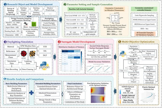
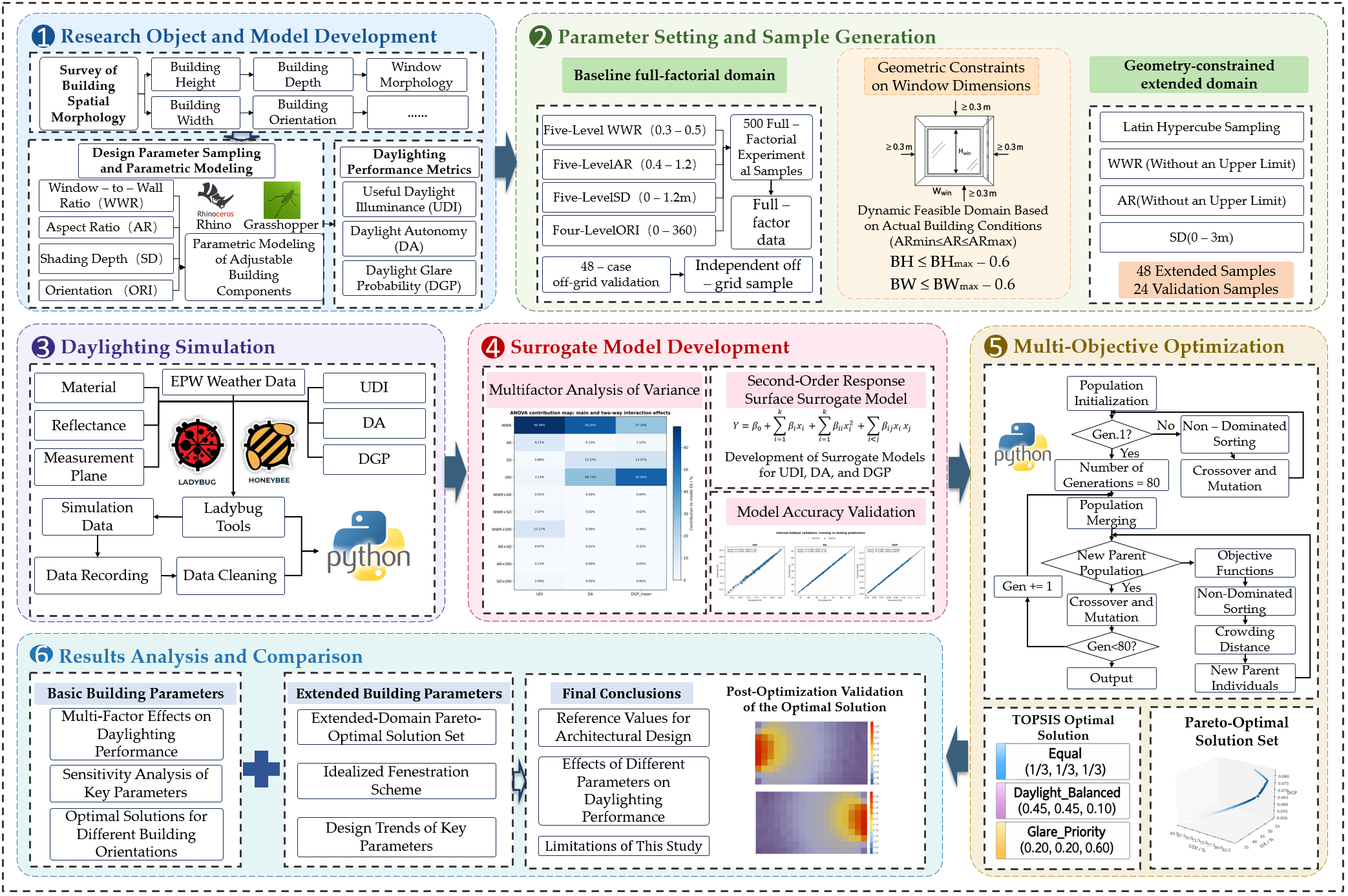
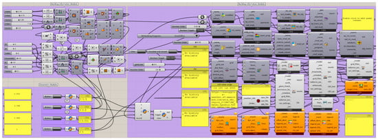
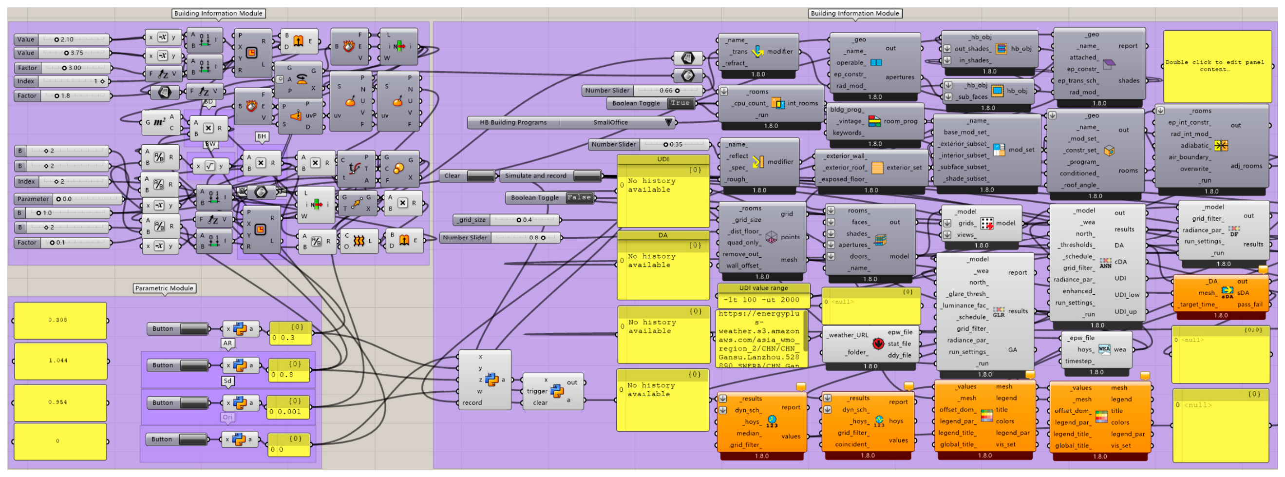
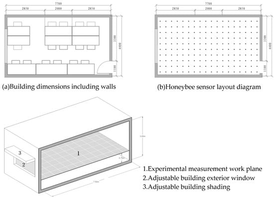
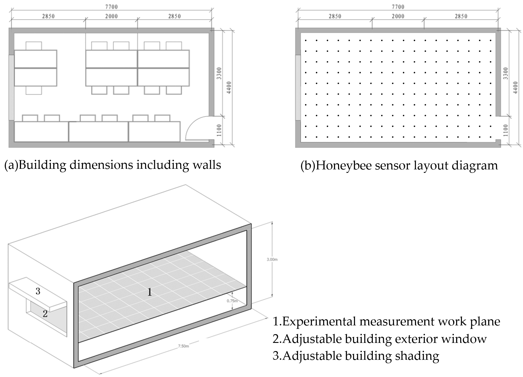
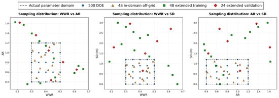
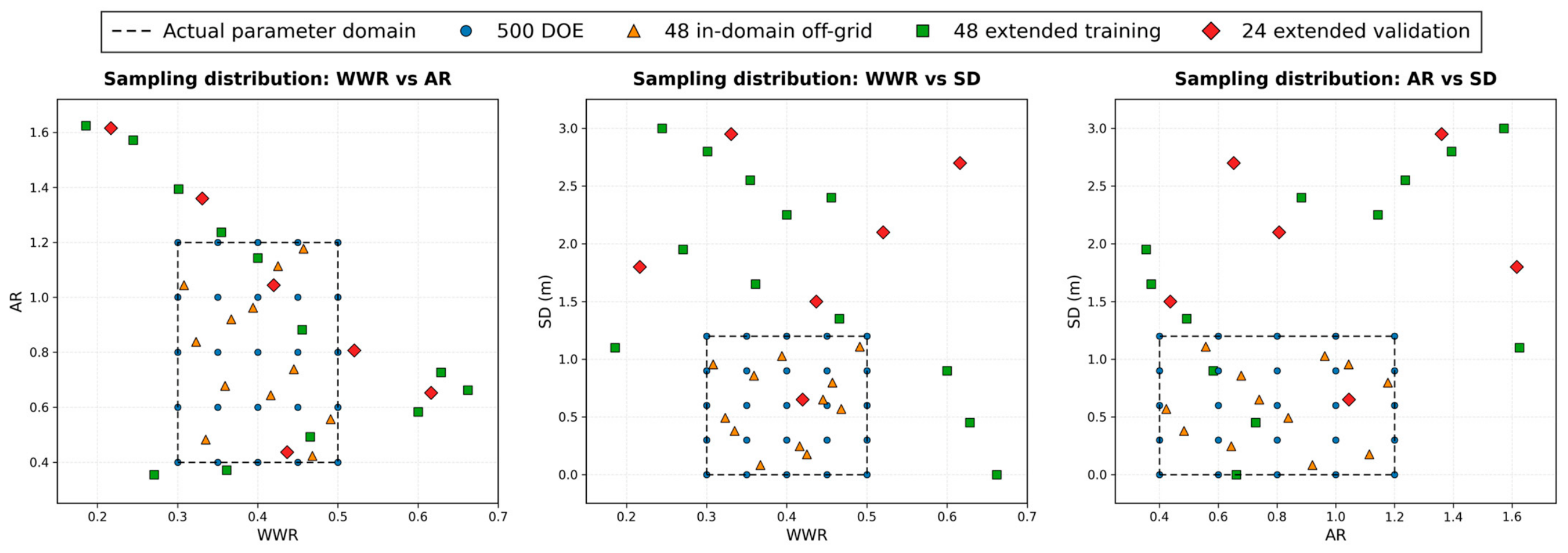
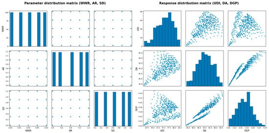
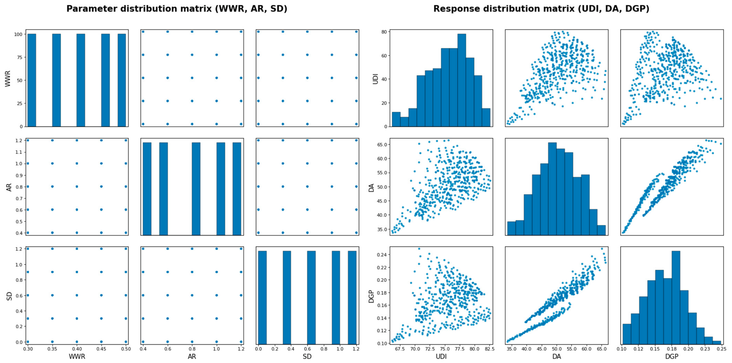
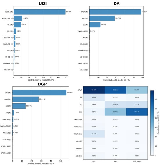
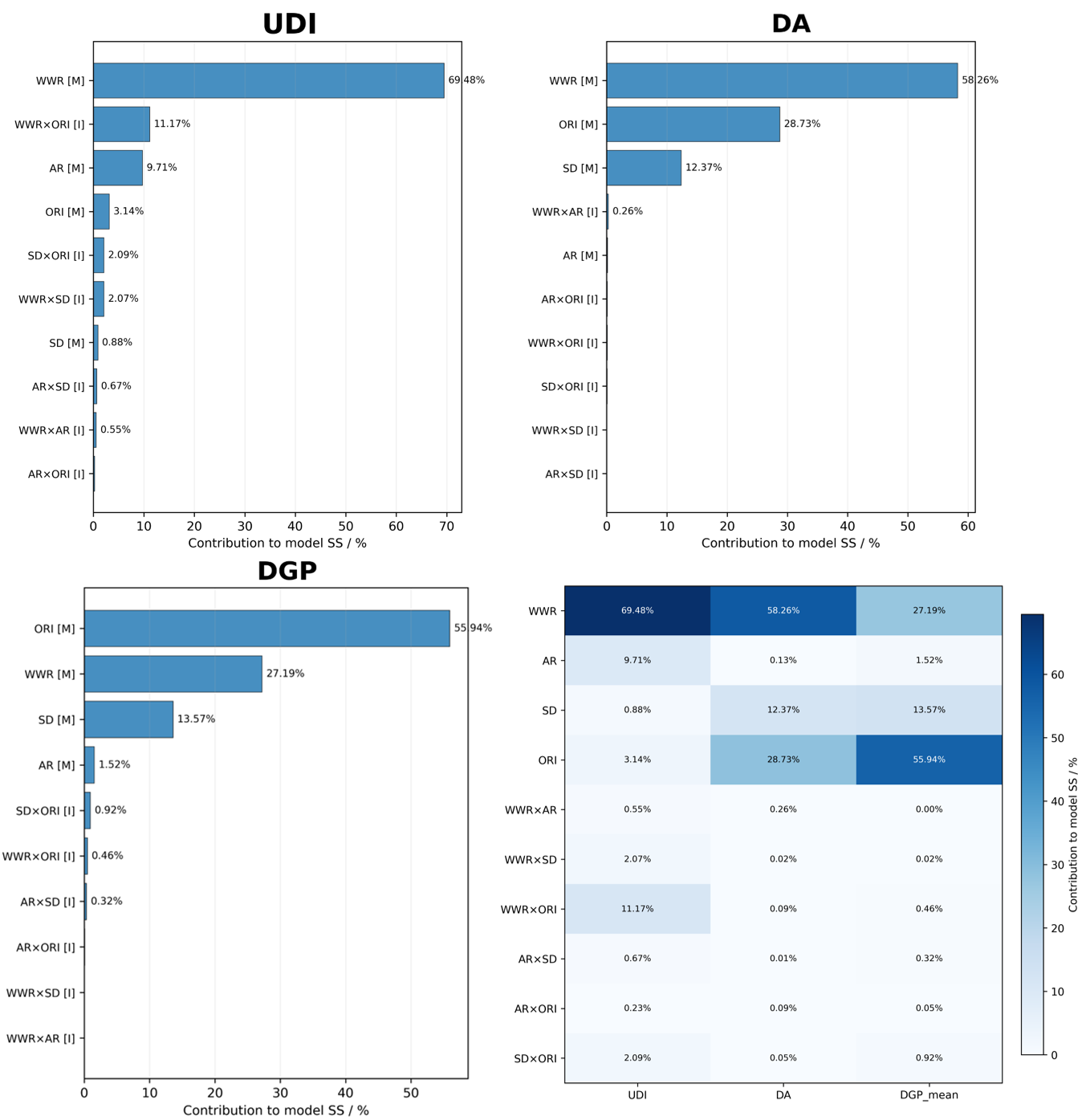
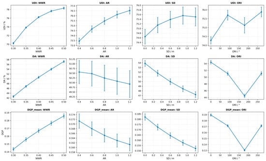
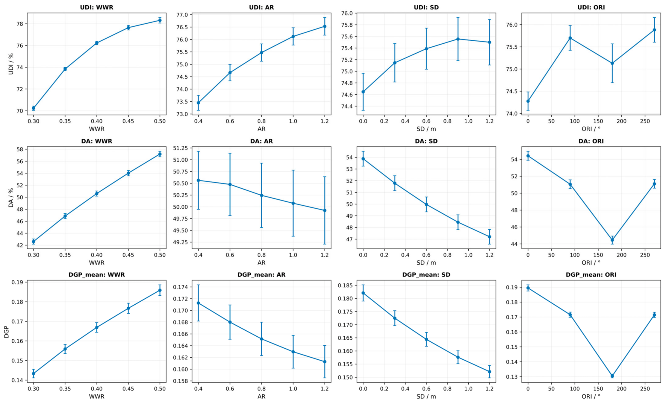
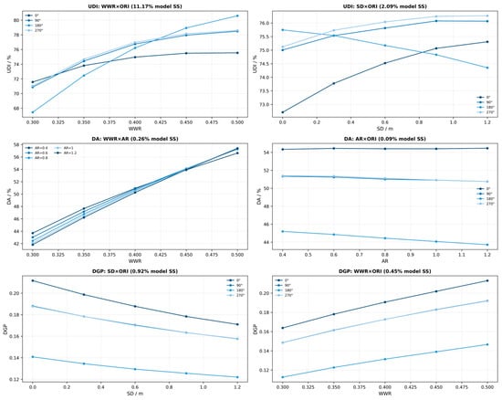
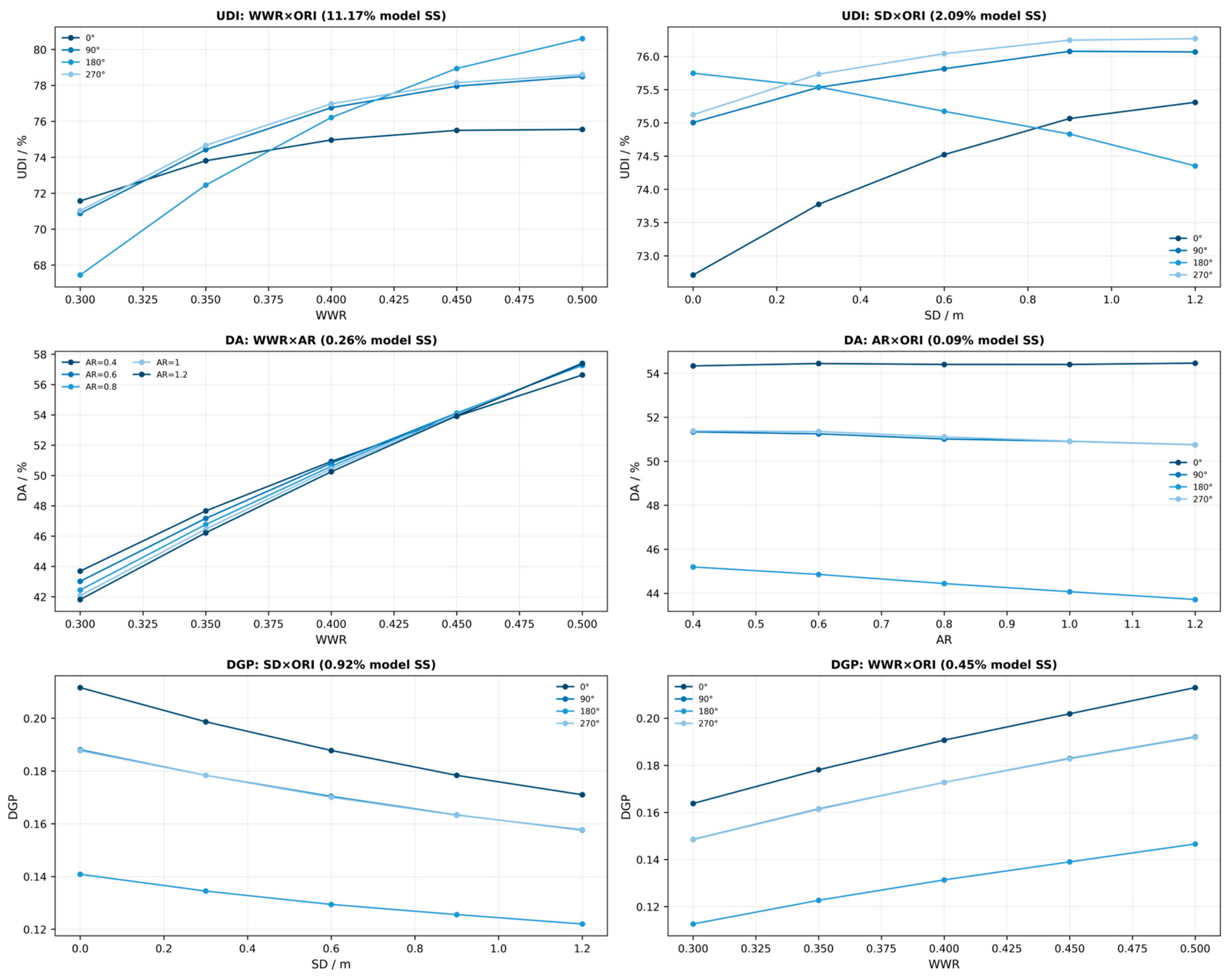
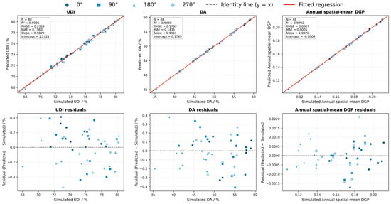
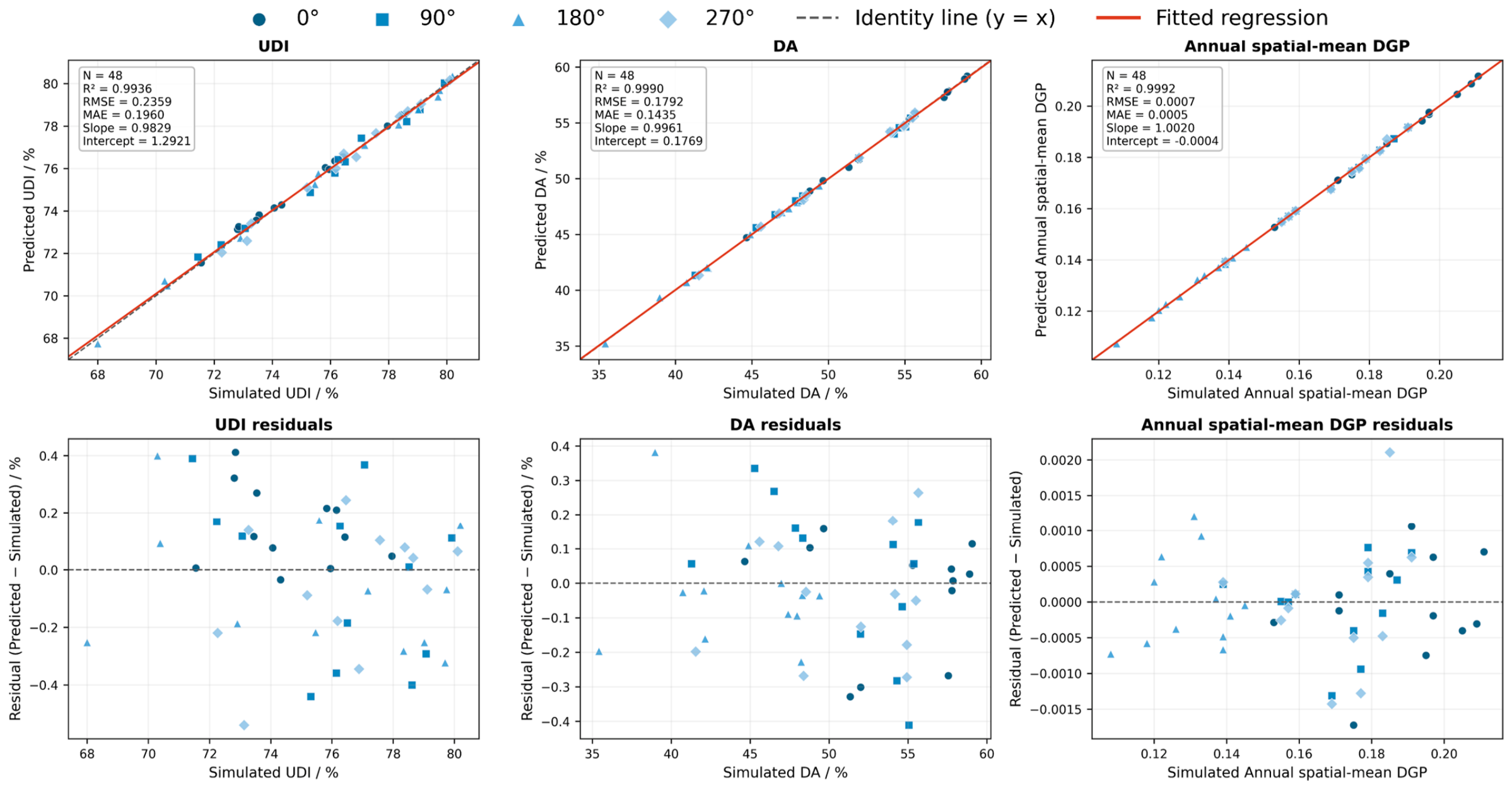
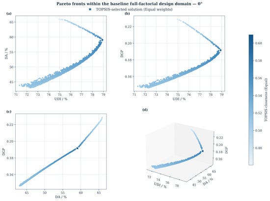
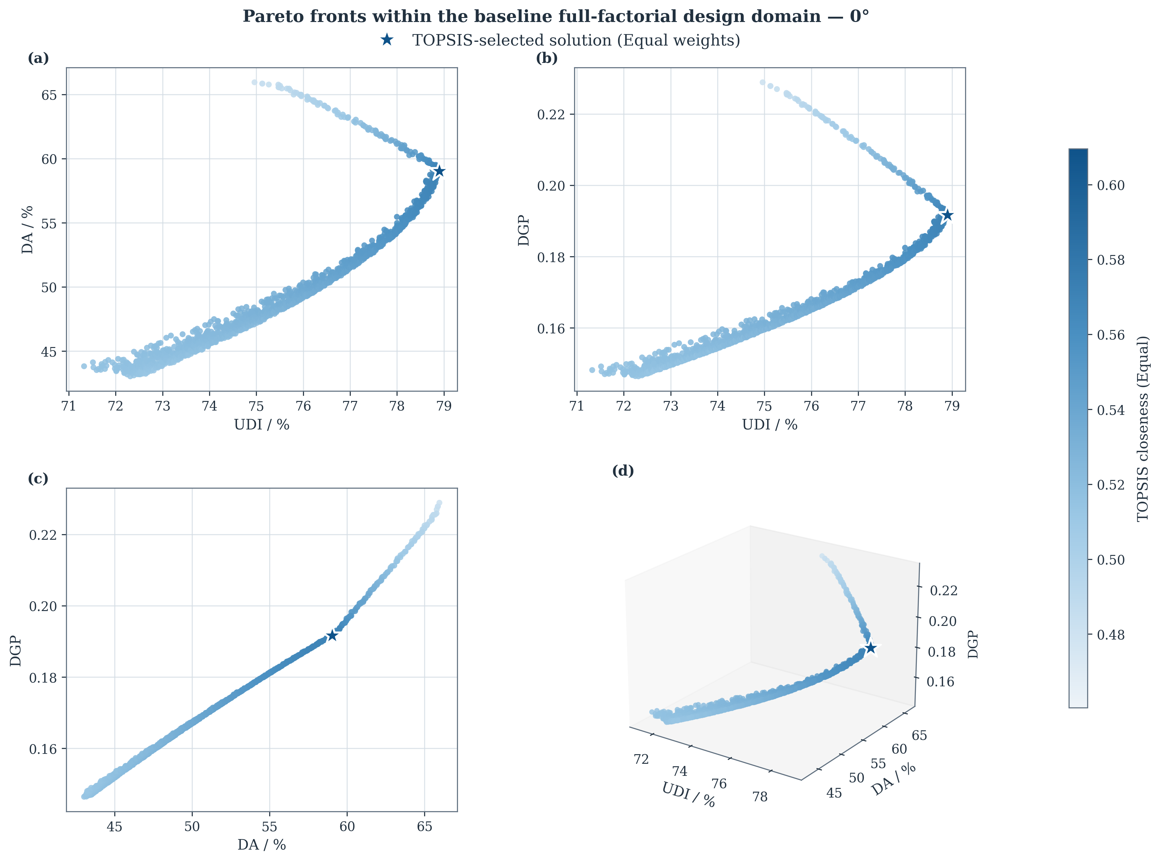
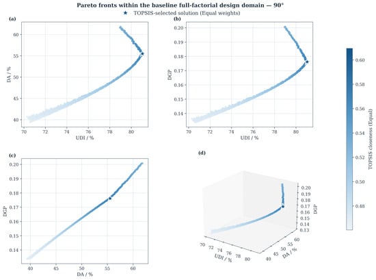
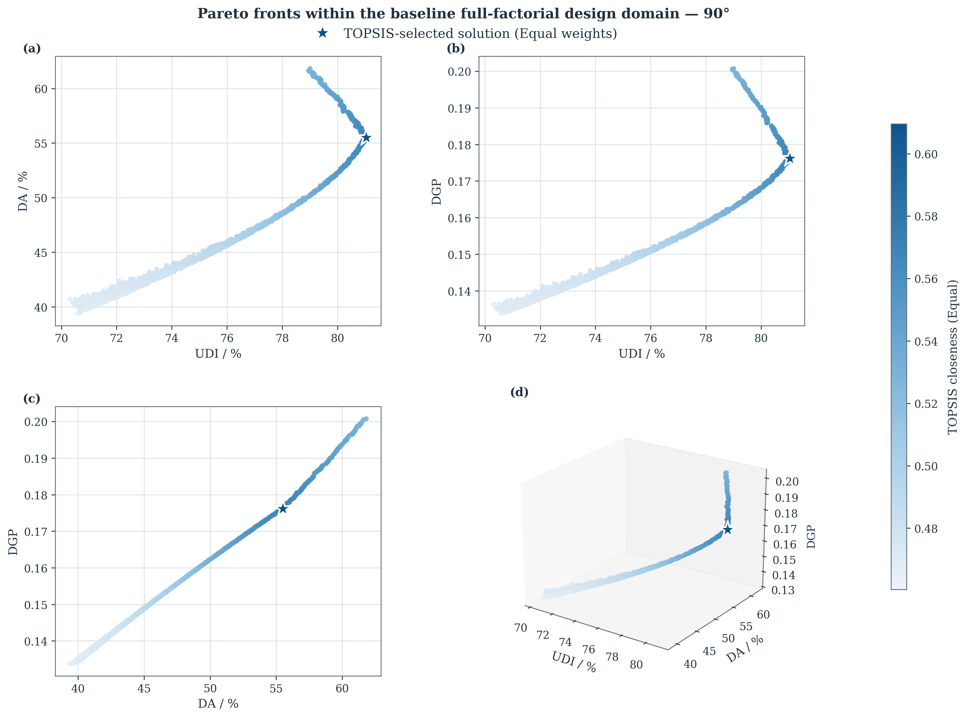
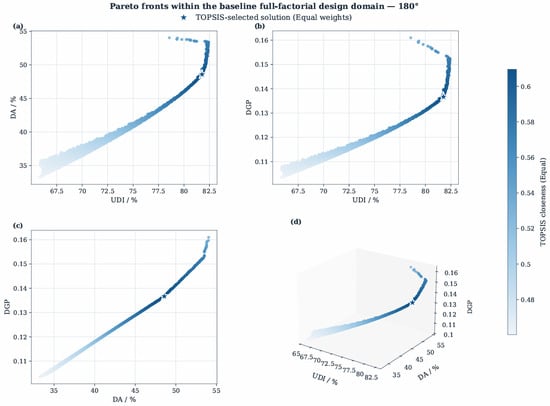
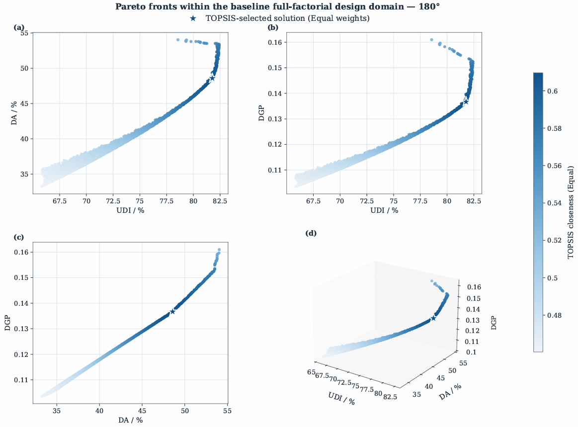
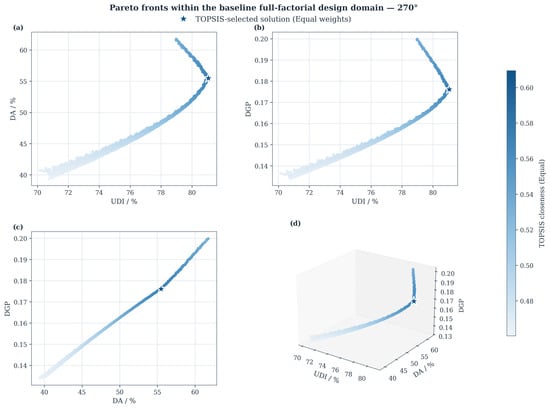
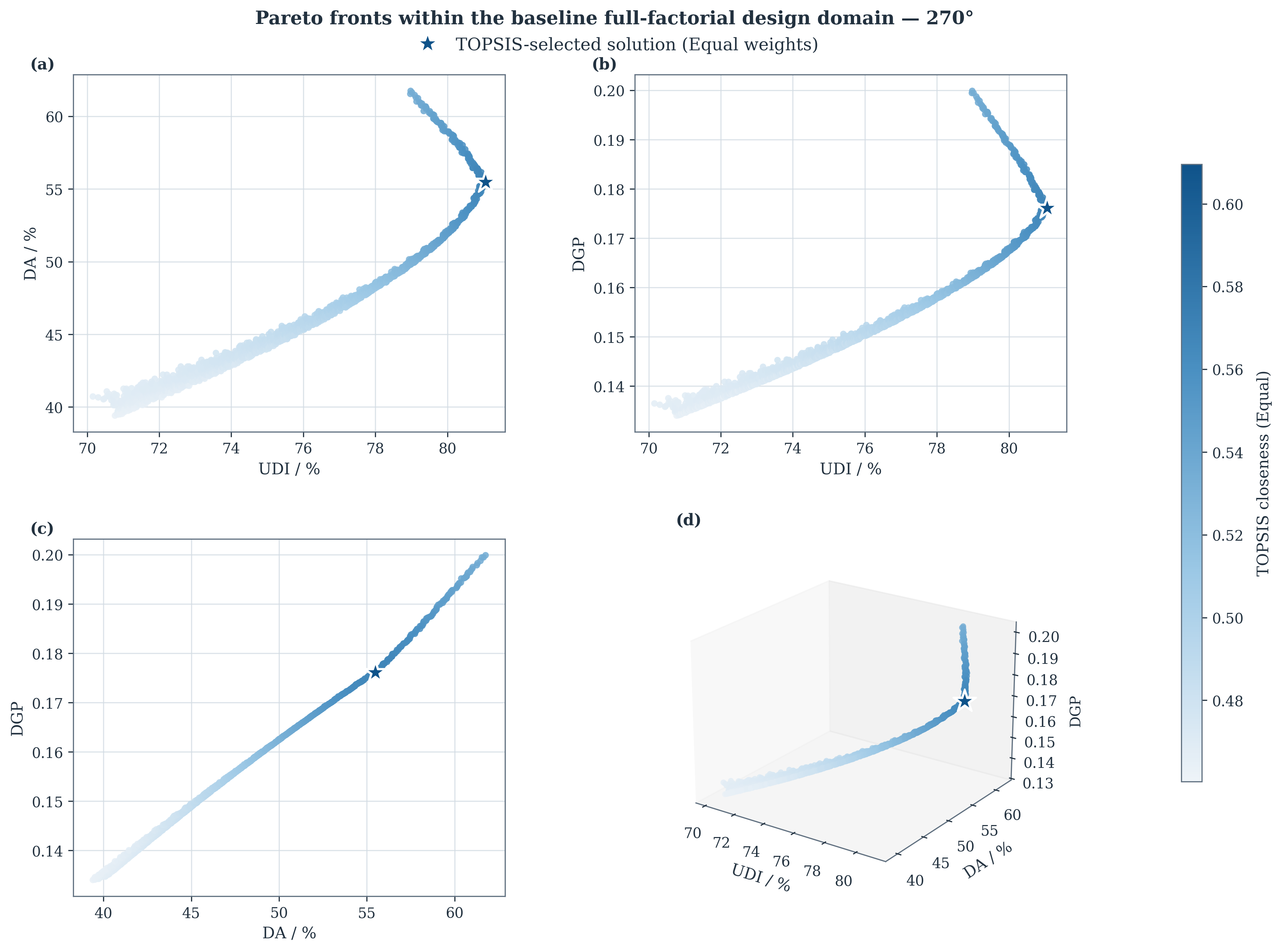
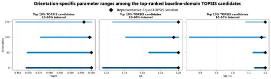
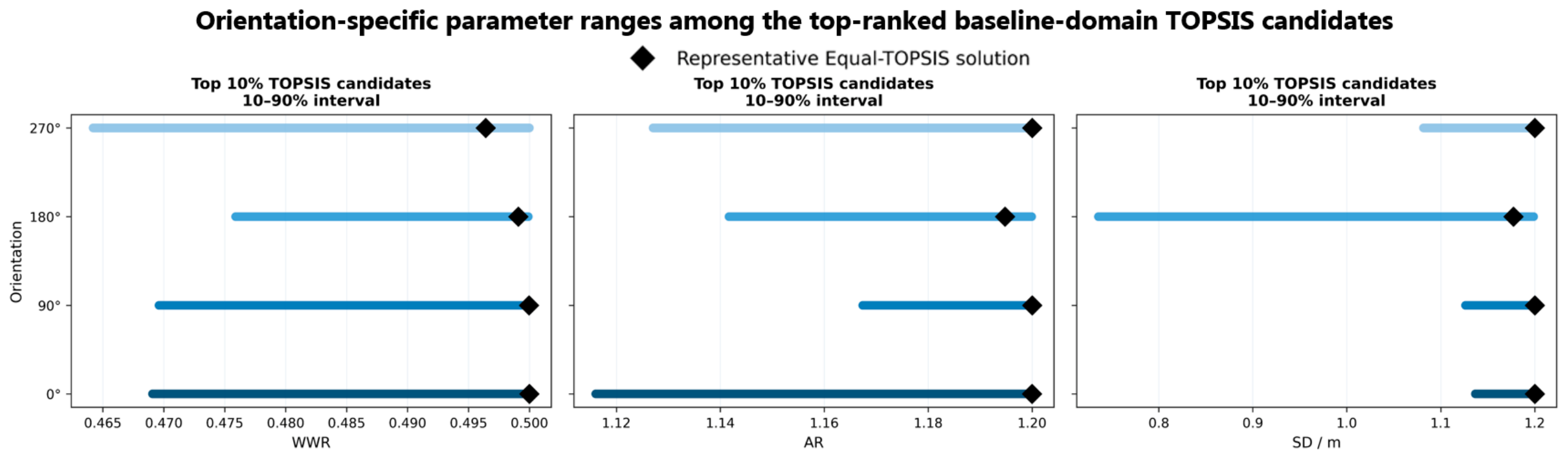
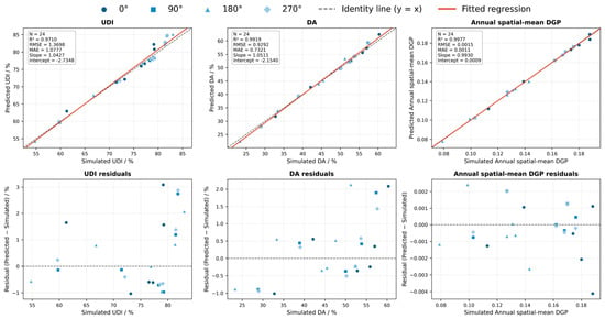
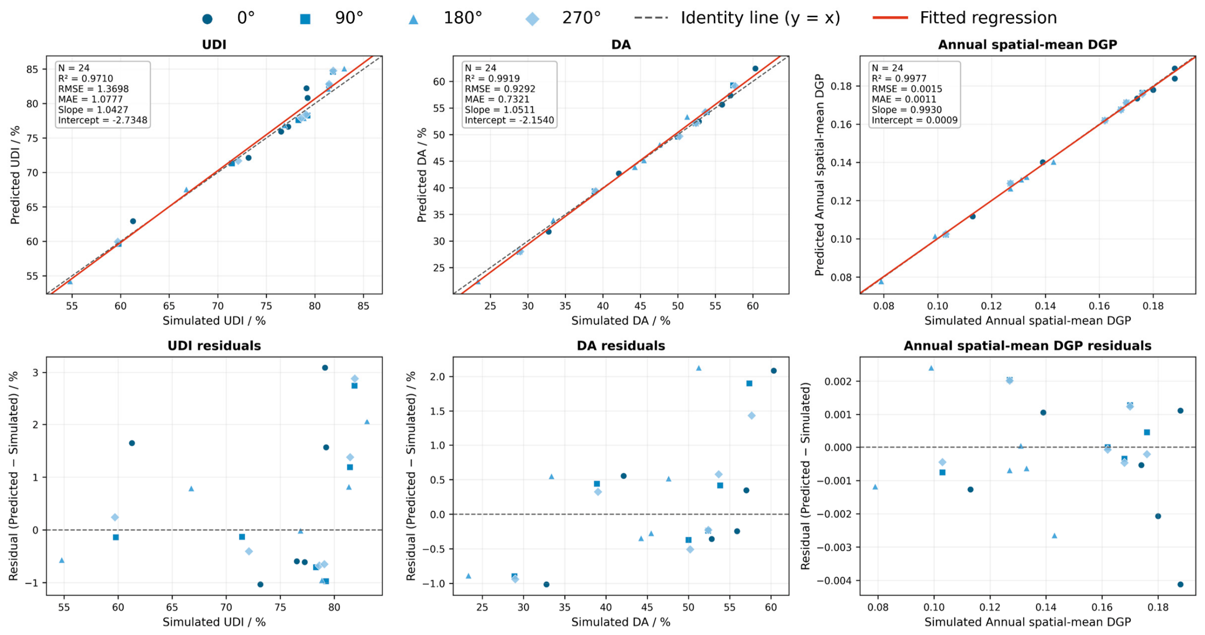
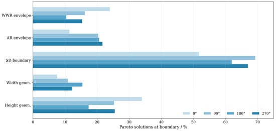
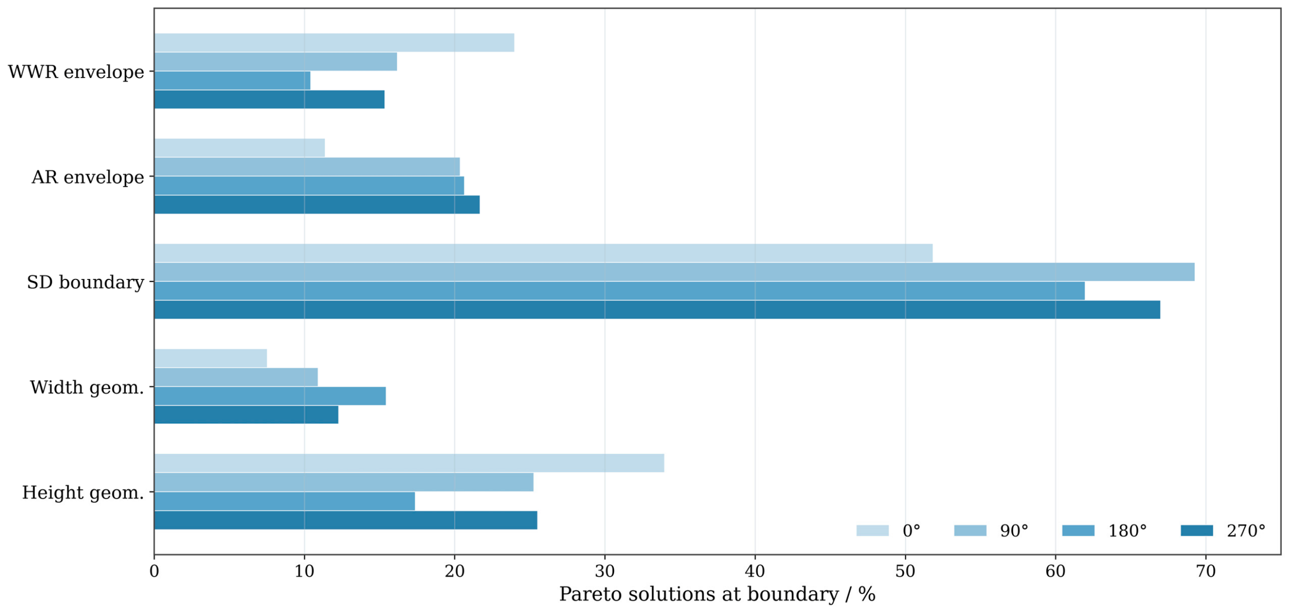
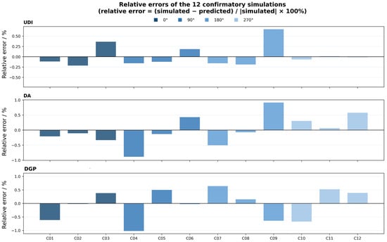
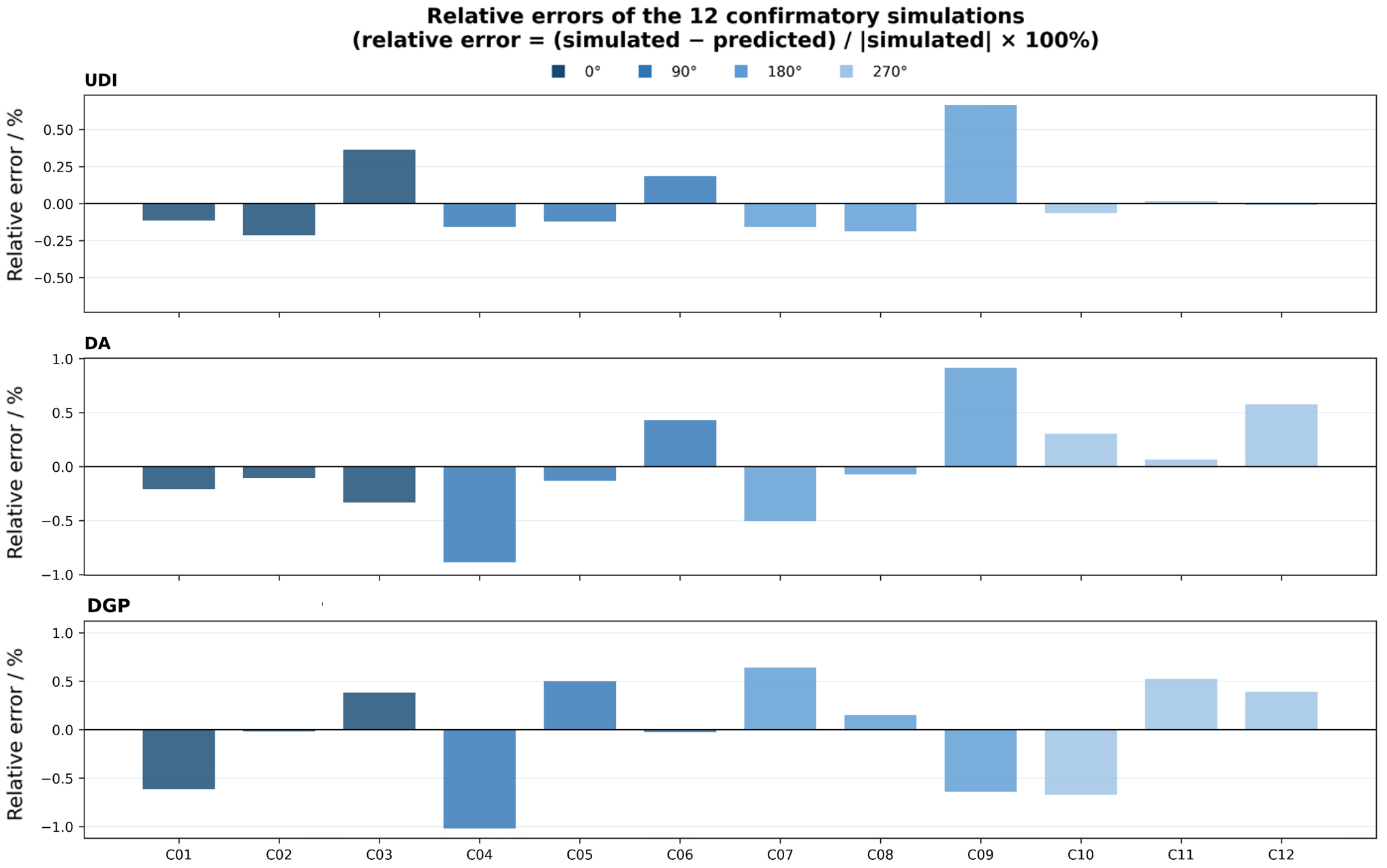
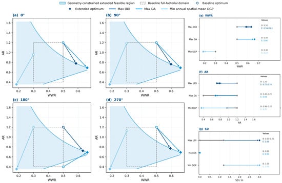
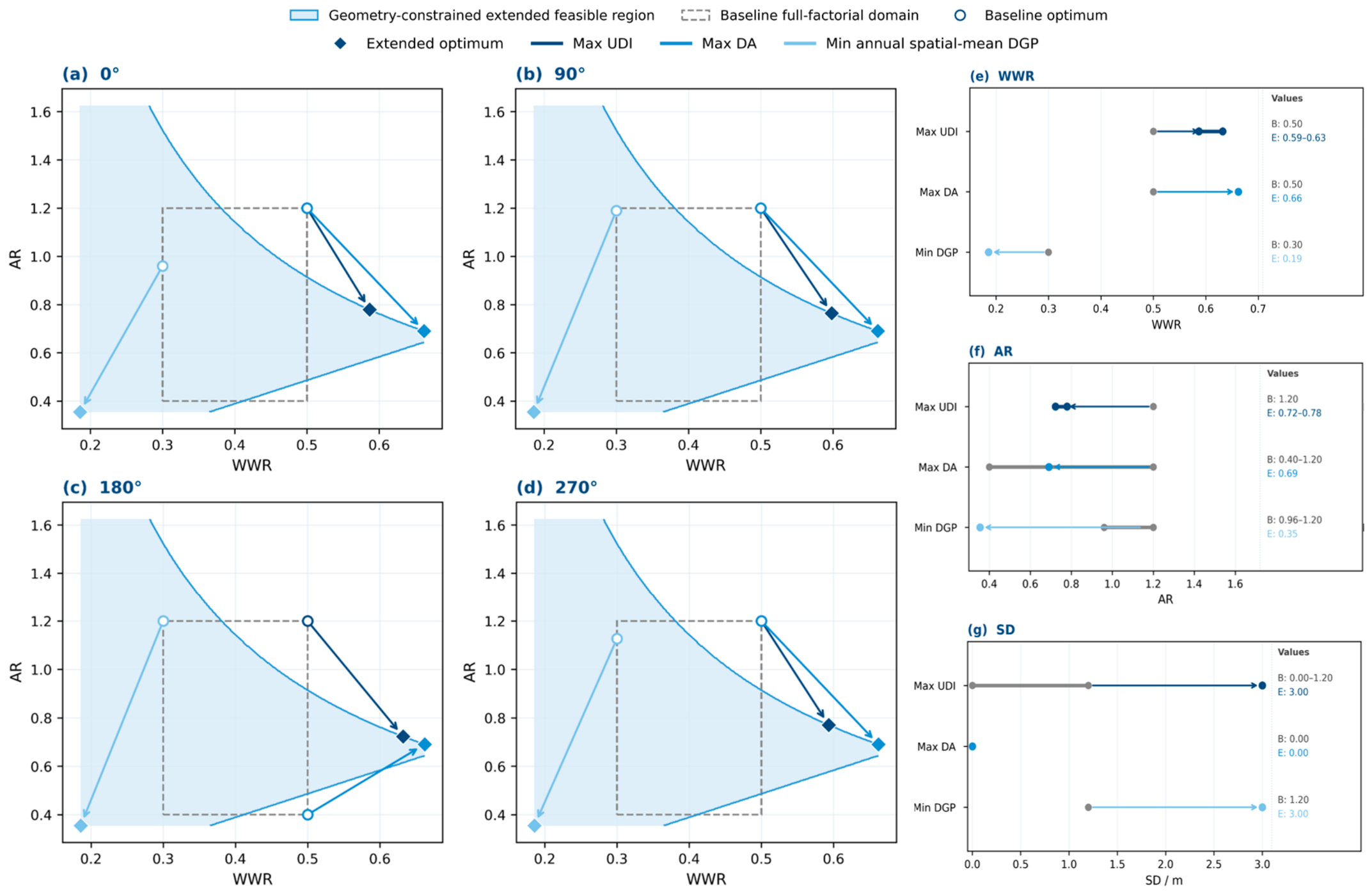

Disclaimer/Publisher’s Note: The statements, opinions and data contained in all publications are solely those of the individual author(s) and contributor(s) and not of MDPI and/or the editor(s). MDPI and/or the editor(s) disclaim responsibility for any injury to people or property resulting from any ideas, methods, instructions or products referred to in the content. |
© 2026 by the authors. Licensee MDPI, Basel, Switzerland. This article is an open access article distributed under the terms and conditions of the Creative Commons Attribution (CC BY) license.