


Abstract
University teaching buildings require design choices that balance energy demand, occupied thermal comfort, useful daylight, and outdoor openness. This study connects these aims to an interpretable shortlist for a teaching floor in Hengyang, China. Four explainable prediction models use a 1000-record simulation archive containing 978 distinct designs and achieve coefficients of determination of 0.935–0.985 for previously unseen design groups. Direct simulations distinguish energy-oriented, thermal-service, and view-oriented alternatives. Compared with the baseline envelope at identical occupied setpoints, a design alternative with manufacturer-linked glazing reduces the ideal-load energy index by 7.62% and discomfort hours by 52.12%, while maintaining useful daylight near 78% and outdoor openness near 9%. Controlled comparisons separate fabric and operating contributions, and catalog substitutions make specification-dependent energy trade-offs explicit. The preferred design depends on the brief: tightening the comfort requirement changes the eligible set and its equal-preference winner. Empirical-error margins guide which predictions merit checking, and direct simulations determine final performance. The workflow gives design teams interpretable environmental alternatives and a reproducible way to update their choice when comfort requirements, priorities, or glazing specifications change.
1. Introduction
Within wider urban energy-efficiency objectives [1], university teaching buildings provide spaces for lectures, independent study and shared campus activities. Their environmental performance depends on coordinated choices about opaque envelopes, glazing, shading and operation. These choices influence heat transfer, solar admission, daylight and access to the outdoor environment together. A larger glazed opening can improve visual access while increasing thermal demand; a deeper louver can reduce solar gains while restricting daylight or sightlines. Evaluating the resulting trade-offs is therefore central to the design and renewal of educational facilities.
Research on educational buildings provides a strong basis for integrated performance assessment. Teaching-building atrium studies combine energy, light, and thermal indicators with optimization and machine learning [2]. Envelope studies compare daylight and energy performance across Chinese climatic zones, while classroom studies examine related trade-offs across United States climates and in hot, dry regions [3,4,5]. Atrium form and future-climate studies extend this analysis to geometry and changing environmental conditions [6,7]. Renovation, kinetic-façade, and bioshading research further demonstrate how educational facilities can be assessed through several environmental objectives [8,9,10]. These applications establish the value of jointly evaluating the spaces, envelopes and service conditions that support teaching activity.
Daylight and outdoor visual access offer complementary information. Frameworks for early-stage building design include view quality alongside energy, daylight and thermal comfort [11]. Fenestration and shading studies likewise examine view-related constraints and objectives [12,13]. A window-view assessment framework distinguishes content, access and clarity [14]. Within this broader visual environment, a geometric openness measure can describe the portion of the outdoor scene accessible through an opening and its shading system. Useful illuminance and unobstructed sightlines need not improve together, so keeping them as separate objectives allows the design team to assess their different responses.
AI applications across infrastructure encompass underground-pipeline recognition from ground-penetrating radar [15], indoor object detection [16], and multi-view road-scene perception [17]. Efficient collaborative perception [18] and cooperative UAV path planning [19] extend this work to distributed sensing and decisions, while visual–inertial SLAM supplies spatial localization [20]. Optimized thermal-process prediction [21], neural PDE solvers [22], and physics-informed tunnel-temperature models [23] illustrate complementary approaches to rapid physical assessment. Engineering learning also includes uncertainty-aware adversarial transfer for fault diagnosis under class imbalance [24] and comparisons of learning-based and physical models for landslide risk [25]. The present study focuses this broader decision-support agenda on environmental trade-offs in campus facilities.
Surrogate models support extensive exploration by learning the relationships between design inputs and simulated performance. Research on building surrogates, simulation-based decision support, and AI-driven design connects sampling, model development, and optimization [26,27,28,29,30,31]. Reviews of building optimization also emphasize the joint choice of variables, simulation assumptions and search strategy [32,33]; evolutionary optimization also addresses complex feasible regions [34]. An accurate predictor supplies rapid estimates, but a design decision also requires alternatives, priorities, and a way to assess the selected design [35]. Explainable AI helps connect learned responses to the physical questions raised by a recommendation [36,37]. BIM-supported design and uncertainty-aware retrofit studies integrate explanation with multiobjective search [38,39], while reviews of interpretable building-energy methods clarify its role in engineering assessment [40]. Benchmarking of expensive building-performance problems also shows why predictive and search behavior should be evaluated together [41].
Three questions guide the study. First, how accurately can four environmental responses be predicted for previously unseen design-input groups? Second, how do envelope, shading and occupied temperature settings shape the available energy, thermal-service, daylight and outdoor-openness trade-offs? Third, how do direct-simulation checks, stated service thresholds, prediction errors and product-linked glazing specifications affect the final design shortlist? These questions are examined for one Hengyang teaching floor using a common climate and operating calendar.
The contribution is a reproducible connection between environmental prediction and explicit design selection. Four response models, group-separated testing, development-fold explanations, and repeated search establish the predictive evidence; direct simulations and controlled comparisons then test the selected design vectors. Preference and sensitivity analyses show how recommendations change with the decision requirements. Figure 1 maps the three study questions to this sequence, and Table 1 identifies the specific distinctions from related educational-building and explainable-optimization studies.
Figure 1.
From environmental evidence to a checked design shortlist. Question 1 is addressed by group-separated testing of four XGBoost 3.0.5 models trained on a 1000-record archive containing 978 distinct input groups. Question 2 is addressed by development-fold TreeSHAPTreeSHAP (SHAP 0.49.1) and repeated NSGA-III search (pymoo 0.6.2) over envelope, shading, and operation. Question 3 is addressed by direct EnergyPlus 23.2/Radiance 6.0.2 checks, TOPSIS preferences, and the controlled/sensitivity analyses in Section 2.6. Each stage supplies evidence for the next: predicted performance, interpretable trade-offs, then checked choices for stated priorities. Solid arrows trace the prediction, search, and candidate-checking sequence; dashed arrows carry grouped evaluation and explanation evidence to the final design shortlist.
Table 1.
Reported scope, numerical evidence, and specific comparison with related studies. Values describe each study’s own case and baseline; they are not a cross-study performance ranking. The comparison distinguishes research scope without treating unexamined features as demonstrated deficiencies.
2. Materials and Methods
The analysis follows the study questions in Figure 1. EnergyPlus 23.2 (U.S. Department of Energy, Washington, DC, USA) supplies thermal demand and hourly indoor conditions; Fanger PMV quantifies occupied thermal service. Radiance 6.0.2 (Lawrence Berkeley National Laboratory, Berkeley, CA, USA) calculates useful daylight, and geometric ray casting calculates outdoor openness. Four XGBoost models then estimate these responses across the design domain. NSGA-III explores their trade-offs, and TOPSIS ranks directly checked alternatives for stated priorities. The controlled comparisons in Section 2.6 test how operating settings, glazing specifications, and decision assumptions affect those recommendations. The recorded analysis environment used Python 3.12.14, NumPy 2.3.5, pandas 3.0.1, scikit-learn 1.7.2, XGBoost 3.0.5, SHAP 0.49.1, Optuna 5.0.0, pymoo 0.6.2, SciPy 1.16.2, and Matplotlib 3.11.2. Full package records are supplied in Supplementary Data and Code.
2.1. Teaching-Floor Model and Operating Scenario
The representative floor is reconstructed from the supplied Honeybee model (honeybee-core 1.64.75, honeybee-energy 1.126.0, and honeybee-radiance 1.66.295) and associated architectural and weather files. It contains 30 unique analytical spaces, with a gross model floor area of 2679.943 m2. Twenty-nine spaces, totaling 2447.543 m2, are assigned occupants and ideal-load conditioning. The remaining space is unconditioned. Coincident duplicates are consolidated before assigning areas, occupants, and sensor weights. Table 2 records the common space program and operating assignments. Figure 2 shows the building and analytical floor.
Table 2.
Geometry, operating scenario, and environmental-response definitions used consistently throughout the experiment. Operating values are declared model assignments. Winter clothing covers December–February, summer clothing June–August, and shoulder clothing the remaining months.
Figure 2.
Study building and analytical floor. (a) Architectural model with the representative floor highlighted. (b) Plan of the 30 unique analytical spaces; 29 occupied and conditioned spaces are shaded blue, and the unconditioned space is shaded grey. The model floor elevation is 6.0 m. The plan shows the geometric and service assignments used in this study.
The common occupancy calendar has teaching activity on weekdays from 07:00 to 11:00, 13:00 to 17:00, and 19:00 to 21:00. Activity is suspended from 15 January through 28 February and from 15 July through 31 August. A 365-day simulation year starts on Sunday and yields 1940 occupied hours in each assigned space. These dates specify the research calendar. The same calendar is used for comfort evaluation and for occupied thermal control.
Occupied heating and cooling setpoints are X17 and X16, respectively. Outside occupied periods, heating and cooling setbacks are 16 °C and 32 °C. The ideal-load systems have no capacity or airflow limits and no economizer. Windows remain closed in this mechanically conditioned scenario. The source infiltration, mechanical ventilation, lighting, and equipment specifications are retained and reported in the operating-parameter table. The activity heat input is 125.604 W per person, obtained from 1.2 met, 58.15 W/m2 per met, and an assumed body area of 1.8 m2. Occupancy availability independently controls the presence of people.
The model uses the supplied Hengyang typical meteorological year. Nominal façade directions are defined in the unrotated reference model; orientation rotates the building and its preserved relative context jointly. Roof and floor boundary assignments represent the selected floor rather than a newly simulated whole-building service inventory.
The assigned occupant density is 0.08 person/m2. Lighting and equipment densities are 8 and 5 W/m2, respectively, with the 1940 h teaching calendar. Infiltration is 0.0006 m3/(s·m2) of exterior surface area and is continuously available. Outdoor-air supply is 0.008 m3/(s·design person), continuously available with demand-controlled ventilation disabled. Lighting and equipment have fixed schedules and no daylight dimming. The energy index therefore captures changes in thermal demand, while UDI describes daylight service. Glazing and shading still affect both solar heat gains and indoor illuminance, but no daylight-controlled lighting-electricity saving is attributed to this model.
2.2. Design Variables and Response Generation
The design domain comprises 16 continuous variables and one categorical shading variable. Continuous variables specify wall solar absorptance, effective wall-layer thickness and conductivity, window U-factor, solar heat gain coefficient and visible transmittance, four façade window-to-wall ratios, louver depth, pitch and tilt, orientation, and cooling and heating setpoints. Window U-factor is passed to the simplified-glazing system in W/(m2·K), including standard surface films. Independent glazing coordinates support the initial parametric search. Product-linked checks in Section 2.6 subsequently replace U-factor, SHGC, and visible transmittance together using manufacturer-published glazing combinations [42].
Wall solar absorptance applies to the exposed exterior finish, while thickness and conductivity apply to the middle effective wall layer. The exterior finish is defined separately from the shared interior finish. Interior material properties and visible reflectances remain fixed, so X1 describes exterior solar absorption rather than a change to the indoor daylight finish. The independent solar/visible optical inputs in the initial archive are distinguished from the linked glazing specifications used in the product-substitution checks.
The study compares exterior horizontal and vertical louvers using common depth, pitch, and tilt variables. The supplied 1000-record Latin-hypercube archive [43] retains its continuous coordinates without resampling. Original category 1 supplies 505 horizontal records; original categories 0 and 2 supply 495 vertical records, defining the present two-category design domain. All thermal and visual responses are generated anew under the common physical model. The 978 distinct complete vectors are simulated once each, and duplicate records receive their corresponding responses. Table 3 gives the input definitions and domains.
Table 3.
Initial parametric design domain. WWR is window-to-wall ratio; SHGC is solar heat gain coefficient. Units are included in dimensional input names. All variables except X11 are continuous. Independent glazing inputs define the search domain; the linked-product substitutions in Section 2.6 provide a separate specification check.
Louver mounting maintains at least 0.05 m clearance from the glazing plane. For a tilt whose projection would extend through that plane, mounting offset is increased by the corresponding depth projection. This keeps the complete louver geometry outside the room across the stated 30–150° tilt domain. All preserved nonconvex detached context polygons are triangulated with unchanged area and material assignments.
EnergyPlus 23.2 [44] evaluates annual thermal response using ConductionFiniteDifference, 20 zone timesteps per hour, FullExterior solar distribution, and PixelCounting shadows. The primary shadow update interval is seven days, and the pixel resolution is 512. Run qualification checks for completion, severe and fatal errors, relevant convergence and shadow warnings, occupied control, and agreement between hourly sums and the rounded annual end-use report. Accepted geometry warnings are reviewed separately. A representative finer-configuration experiment assesses numerical sensitivity.
Radiance 6.0.2 [45] evaluates daylight using a Perez annual sky matrix and the daylight-coefficient method. The primary sky subdivision density is two. Coefficients use three ambient bounces, 2048 ambient divisions, and a minimum ray weight of 10−5. Work-plane sensors have 1 m nominal spacing and are 0.8 m above each floor. The RGB irradiance-to-illuminance coefficients are 47.4, 119.9, and 11.6. A density-four calculation with four ambient bounces and 4096 ambient divisions assesses representative numerical sensitivity. These settings and the full per-sensor annual values are retained with the calculation records.
2.3. Performance Measures
The ideal-load energy index, denoted EUI, is the annual sum of ideal supply-air heating and cooling thermal demand plus scheduled lighting and equipment electricity, divided by the unique gross model floor area. It is used consistently to compare the simulated designs. Heating, cooling, and electrical components are also reported separately; EUI is not an estimate of purchased HVAC electricity or utility bills. Section 2.6 additionally evaluates an electricity proxy by dividing heating and cooling demand by explicitly assumed equipment coefficients of performance before adding the electrical end uses. The ideal-load system supplies thermal demand at ideal efficiency without a detailed plant or distribution system [46].
DCH counts occupied hours outside a stated thermal-service tolerance in the 29 controlled spaces. For space i, floor area Ai and scheduled occupancy indicator Oit weight the hours for which |PMVit| exceeds 0.85. The area-weighted count is reported in hours, and its annual fraction is DCH/1940. The PMV model [47], implemented in ladybug-comfort 0.19.11, uses simulated air temperature, mean radiant temperature and relative humidity, with 1.2 met, 0.1 m/s and clothing of 1.0 clo in December–February, 0.5 clo in June–August and 0.75 clo in the remaining months. The |PMV| = 0.85 boundary corresponds to approximately 20.25% instantaneous predicted dissatisfaction under the PMV–PPD relation. It is a declared study tolerance. The annual 20% discomfort-hour screen is a separate preference; neither quantity is presented as an ASHRAE 55 compliance test. Sensitivity calculations also use |PMV| limits of 0.50 and 0.70; the former is the PMV-zone boundary described by the CBE tool [48], and the latter is an intermediate sensitivity level.
UDI [49] uses 3650 h corresponding to daily 08:00–18:00 local standard time. It averages the fraction of grid-hour illuminances between 100 and 3000 lx within each space and then weights the space results by floor area. This daylight-service window covers daylight availability throughout the year, including vacation dates. The retained annual matrices also support the same 100–3000 lx band during the 1940 h teaching calendar and the alternative 300–2000 lx band during the primary daylight window. These paired results assess the consequences of both time-window and illuminance-band choices.
VP is a geometric measure of outdoor openness. From a grid 1.2 m above the floor, 512 fixed equal-solid-angle Fibonacci directions sample the full sphere. A ray is counted if it meets no opaque model or context surface within 200 m. Glazing is transparent for this geometric calculation. The sensor average is area-weighted over the 30 spaces. Quadrature directions co-rotate with the building and its relative context to preserve the geometric measure under joint orientation changes. VP is reported as the percentage of unobstructed rays and complements the illuminance-based UDI objective.
2.4. Surrogate Development and Explanation
Exact duplicate input vectors are assigned a shared group identifier before any data partitioning. A fixed group-shuffle split with seed 42 reserves 20% of the groups for testing. Continuous inputs are standardized using statistics fitted only within the applicable training partition, and the two shading categories are represented by fixed indicator columns. The saved assignments identify every record in the development and test partitions.
Each XGBoost [50] response model receives 50 Optuna [51] trials using a seed-42 TPE sampler and three group-separated development folds. The selected configuration minimizes mean validation RMSE in the original engineering units. Search ranges and the complete trial histories are saved. EUI uses a logarithmic response link. DCH uses a logit link with a physical upper bound of 1940 h, the total annual occupied duration; UDI and VP use logit links relative to 100%. The fraction transform has a boundary epsilon of 10−5. Inverse links preserve the physical response ranges during search.
The frozen development models are evaluated on the reserved test groups using R2, RMSE, and MAE in the original units. Fixed Ridge and Random Forest comparators use the same partition, input encoding, and response links. These comparators assess the selected XGBoost workflow against two specified reference configurations. Test predictions are saved before production XGBoost models are refit on all 1000 records. Development and production models, scalers, and fold assignments are retained separately.
TreeSHAP [52] explains the transformed model outputs. Contributions for the two shading indicators are summed into X11, and additivity is checked against the transformed prediction. Five group-separated development fits at the selected configuration provide development-fold explanations, feature rankings, and pairwise Spearman correlations. Equal importance values receive average ranks, including zero-importance ties. These descriptive stability fits complement the independently reserved prediction test. Table 4 summarizes the development, testing, and explanation protocol.
Table 4.
Surrogate development, independent testing and explanation protocol. Fixed comparator configurations, target-specific search ranges, selected hyperparameters, and trial histories are supplied in Supplementary Data and Code.
2.5. Search and Preference Selection
NSGA-III [53], implemented in pymoo [54], minimizes the four-objective surrogate vector in Equation (1) over the input domain X. The vector x contains the 17 design inputs, and each component is a production-model prediction. Predicted EUI and DCH are minimized; predicted UDI and VP are negated to express maximization in cost form.
The implemented objectives are linearly normalized using the minimum and range of each cost-oriented response in the complete simulation dataset. These constants remain fixed for all generations and seeds. The search uses a population of 100, 84 Das–Dennis reference directions with six partitions, simulated binary crossover with mating probability 0.9, variable probability 0.5 and distribution index 15, and polynomial mutation with individual probability 0.7, variable probability 1/17 and index 20. Categorical repair rounds X11 to the two allowed shading levels. Each of the three seeds, 42, 52, and 62, is run for 200 generations. A reference vector of [1.1, 1.1, 1.1, 1.1] is used for hypervolume diagnostics in this fixed normalization. Every generation’s population, evaluated vectors, and convergence summaries are saved. The final candidate set is the nondominated union of all three final retained populations after exact duplicate vectors are removed. Population hypervolume and nondominated counts are computed from every nondominated retained member at each generation. Table 5 summarizes the search and preference settings.
Table 5.
Repeated search and preference settings. Weight order is EUI, DCH, UDI, and VP. The environmental screen represents study preferences; numerical acceptance and occupied setpoint control are checked separately.
Five TOPSIS [55,56] profiles describe equal preference and individual emphasis on energy, thermal service, daylight, and visual permeability. The emphasized criterion has weight 0.55, and each remaining criterion has weight 0.15; equal preference assigns 0.25 to each. For the set being ranked, each response is divided by the square root of the sum of its squared values and multiplied by its criterion weight. In Equation (2), zij is this weighted normalized response for design i and criterion j; zj+ and zj− are the ideal and anti-ideal values. The ideal minimizes EUI and DCH and maximizes UDI and VP. Di+ and Di− are the corresponding Euclidean distances, and a larger closeness Ci indicates a higher preference rank.
Direct reference simulations cover the five full-front profile winners, their highest-ranked alternatives passing the predictive service screen, the four objective extrema, and the candidate closest to the normalized ideal. Duplicate selections are calculated once. The initial screen uses occupied discomfort no greater than 20%, UDI no lower than 60%, and VP no lower than 5%. These values define a study scenario: at least 80% of area-weighted occupied hours within the declared thermal tolerance, a 60% area-weighted useful-daylight fraction, and a minimum full-sphere openness preference. They are not building-code limits. The screen is reapplied to direct-simulation outputs before ranking the checked shortlist. Section 2.6 varies all three preferences and the PMV tolerance. Numerical-run quality and occupied temperature control are checked separately.
A midpoint design without exterior louvers provides a common simulation baseline using the same geometry, climate, service calendar, and ideal-load system. Its continuous envelope variables are at domain midpoints, orientation offset is zero, and occupied cooling/heating setpoints are 26/20 °C. Initial comparisons quantify the combined effects of envelope, shading, and occupied-setpoint changes. The controlled comparisons in Section 2.6 separate these effects for selected designs. Candidate prediction errors, ranking changes, baseline differences, and calculation durations are reported. A 1771-point grid of nonnegative weights summing to one, in increments of 0.05, maps winner regions within the fixed checked, screen-passing set.
2.6. Controlled Comparisons and Decision Sensitivity
Four directly checked designs (D102, D221, D239 and D241) are recalculated after resetting occupied cooling/heating setpoints to the common baseline values of 26/20 °C. All other inputs are retained, including geometry, glazing, shading, weather, and schedules. Daylight and openness are reused because this control change does not affect their geometry or optical inputs. For D102 and D221, the baseline envelope is also evaluated at each design’s original settings. Together with the existing baseline and joint design, these cases form a two-factor envelope/shading-by-operation comparison, including an interaction term. This is a controlled ablation of selected designs, not a new fixed-setpoint global optimization.
Two glazing checks retain linked catalog tuples [42]: product A, Solarban 90 on Starphire/Starphire, has U = 1.36 W/(m2·K), SHGC = 0.23 and VT = 0.54; product B, Solarban 70 on clear/clear glass, has U = 1.35 W/(m2·K), SHGC = 0.28 and VT = 0.64. Both are 4/12/4 mm units with a 90% argon gap. D221 uses A and D239 uses B, with their other original inputs unchanged. Manufacturer-published NFRC winter-night center-of-glass values are used as linked simplified-glazing inputs, without a frame model. Thermal and annual daylight responses are recalculated; transparent-ray openness is unchanged. These tests evaluate catalog-representative alternatives without identifying the original independent tuples as purchasable products. The glazing performance tables are supplied by Vitro Architectural Glass (Pittsburgh, PA, USA).
Energy outputs were reported separately as ideal heating and cooling demands, scheduled lighting electricity, and equipment electricity. An assumed-efficiency comparison converted the thermal demands using cooling COPs of 2.5/3.5/4.5 and heating COPs of 2/3/4, giving nine combinations. Lighting and equipment remained unchanged; the scenarios represent a constant-efficiency electricity proxy, without installed-system or daylight-dimming simulation.
Sensitivity was evaluated at absolute PMV limits of 0.50/0.70/0.85 crossed with discomfort ceilings of 15/20/25%, UDI floors of 55/60/65% and openness floors of 4/5/6%. Hourly discomfort was area-weighted over 29 conditioned spaces, each with 1940 occupied hours. Eligibility and reference-set TOPSIS rankings were recalculated for all 81 scenarios, retaining cases with no eligible design.
Empirical prediction-error bands were calibrated from archived development-fold residuals after collapsing 804 records to 782 input groups, then evaluated on 196 reserved test groups without refitting. Upper DCH and lower UDI/openness bounds defined a conservative screen; full-front TOPSIS normalization was retained for verification priorities. These empirical bands guide reference checks and carry no guaranteed post-optimization coverage claim. Empirical bands use the absolute-residual order statistic at ceil((782 + 1)p), with p = 0.90 or 0.95, and are clipped to physical response bounds. For the added conservative verification priorities, TOPSIS is calculated on all 256 margin-adjusted vectors, and eligibility is then applied, preserving the original full-front selection scope. The final reference shortlist is normalized separately after screening, as in Section 2.5. Here p denotes the target empirical coverage probability.
3. Results
The results follow the three research questions. After the simulated response space is described, Section 3.2 addresses prediction for unseen input groups (Question 1), and Section 3.3 and Section 3.4 explain the design trade-offs and their drivers (Question 2). Section 3.5, Section 3.6, Section 3.7 and Section 3.8 examine how direct checks, stated preferences and sensitivity analyses affect the shortlist (Question 3).
3.1. Simulated Response Space
The completed archive contains 1000 design records representing 978 distinct input vectors. All distinct vectors produced qualified thermal, daylight, and openness outputs, with no severe or fatal EnergyPlus errors in accepted runs. Figure 3 describes the four environmental responses separately.
Figure 3.
Simulated response distributions for the 1000 design records: (a) ideal-load energy index (EUI), (b) occupied discomfort hours (DCH), (c) useful daylight illuminance (UDI) and (d) visual permeability (VP). Repeated input records share their corresponding response; the archive contains 978 distinct simulated vectors. EUI combines ideal heating/cooling thermal demand and scheduled electricity, not purchased HVAC electricity. DCH is area-weighted over 29 occupied spaces; UDI and VP over all 30 analytical spaces.
Energy: the ideal-load energy index ranges from 88.53 to 157.78 kWh/(m2·year), with a mean of 111.92. Fixed lighting and equipment electricity contribute 23.03 kWh/(m2·year). Design-dependent differences therefore arise from thermal demand.
Thermal service: occupied discomfort ranges from 3.30 to 1306.95 h, with a mean of 702.30 h. These differences express how the envelope and occupied controls interact under the declared PMV tolerance.
Daylight: UDI ranges from 7.19% to 83.14%, with a mean of 65.13%. The response measures useful illuminance during the specified daylight-service window, independently of lighting-electricity savings.
Outdoor openness: VP ranges from 0.11% to 9.84%, with a mean of 3.78%. This geometric measure exposes obstruction differences that are not captured by useful illuminance alone.
Sixty distinct archive designs meet the three initial service targets together. These designs establish that useful compromises exist within the sampled domain and motivate the subsequent search. Joint screening matters because good daylight alone does not establish acceptable thermal service or outdoor openness.
3.2. Prediction on Independent Input Groups
The group-separated partition contains 804 development records in 782 input groups and 196 test records in 196 groups. XGBoost achieves test R2 values of 0.935 for EUI, 0.985 for DCH, 0.951 for UDI, and 0.963 for VP (Figure 4). Their corresponding RMSE values are 2.739 kWh/(m2·year), 43.165 h, 4.746 percentage points, and 0.468 percentage points. The four models provide consistently useful predictions across responses with different physical ranges and distributions.
Figure 4.
XGBoost predictions for the 196 reserved test records, representing 196 input groups: (a) EUI, (b) DCH, (c) UDI and (d) VP. The dashed line denotes agreement between prediction and simulation. R2, RMSE, and MAE are calculated in the original response units, with RMSE and MAE in kWh/(m2·year), hours, and percentage points, respectively. These predictions come from the development fits saved before the full-data production fits.
Under the specified comparison configurations, XGBoost has the highest R2 and lowest RMSE and MAE for every response (Table 6). Ridge performs comparatively well for EUI (R2 = 0.881), and Random Forest for DCH (R2 = 0.963). For UDI and VP, Random Forest achieves R2 = 0.915 and 0.901, compared with XGBoost values of 0.951 and 0.963. Both tree ensembles outperform Ridge on these visual responses, consistent with nonlinear effects of louver type and dimensions. These results support the target-specific XGBoost models used for the subsequent four-objective design search.
Table 6.
Prediction performance on the same 196 held-out input groups. Errors are in the response units shown; pp denotes percentage points. XGBoost configurations are selected on development folds, while Ridge and Random Forest use the stated fixed configurations.
3.3. Predicted Alternatives and Design Trade-Offs
The nondominated union of the three final search populations contains 256 distinct predicted alternatives. Figure 5 displays the thermal–energy and daylight–openness trade-offs together with five representative objective profiles. The predicted equal-preference and daylight-emphasis profiles select D221, energy emphasis selects D102, thermal emphasis selects D239, and view emphasis selects D241. The low-energy extremum D001 is included to make the cost of prioritizing a single objective visible. These identifiers refer to one retained union and are used consistently in the subsequent reference checks.
Figure 5.
Predicted trade-offs among the 256 alternatives in the pooled nondominated front: (a) EUI–DCH, (b) UDI–VP and (c) representative objective profiles. Grey points show the full front; colors identify the five displayed designs. In (c), each objective is normalized by its minimum and range within those five designs and oriented so that higher values are more favorable. This display normalization is separate from the fixed search normalization. Directly simulated reference outputs are reported in Section 3.5.
The representative input vectors in Table 7 make the alternatives interpretable as design choices. D221 and D239 combine horizontal louvers with approximately 0.10–0.11 m depth, 1.82–1.87 m pitch, and tilt near 149°. Their occupied cooling setpoints are approximately 24.1–24.4 °C, and heating setpoints are approximately 21.6–21.7 °C. D102 uses smaller south and north opening ratios, approximately 0.378 and 0.284, and a 25.1 °C cooling setpoint. D241 allocates larger south and west openings, approximately 0.739 and 0.763. D001 instead combines close louver spacing, approximately 0.179 m, with a 27.9 °C cooling setpoint and an 18.4 °C heating setpoint. The alternatives consequently embody different operational as well as envelope strategies.
Table 7.
Representative vectors for the five designs in Figure 5. Definitions and units are in Table 3. Display values are rounded; full-precision vectors are supplied in Supplementary Data and Code.
3.4. Explanatory Structure and Stability
The development-fold TreeSHAP patterns distinguish operational and geometric drivers (Figure 6). Cooling setpoint accounts for 21.2% of mean absolute EUI contribution and 50.6% of DCH contribution. Heating setpoint contributes a further 23.0% to DCH, while window SHGC contributes 14.9% to EUI. These relationships connect the modeled thermal response to occupied temperature control and solar admission. For daylight, louver pitch, depth, and tilt account for 40.8%, 19.9%, and 19.2% of the contribution, respectively. For VP, their corresponding shares are 39.6%, 22.6% and 15.9%. The dominant visual inputs therefore form a coherent shading-geometry group.
Figure 6.
Development-fold TreeSHAP evidence. (a) Feature contribution shares for the four transformed response models, calculated as mean absolute SHAP values across the 804 development records and normalized within each target. Each record is explained by a model fitted to other development groups at the selected configuration; the two shading-indicator contributions are combined as X11. (b–d) Dependence profiles for the leading continuous input of the VP, UDI and DCH models, respectively. Colors distinguish exterior horizontal and vertical louvers. The dark line joins the input and SHAP medians within ten equal-width input bins. The dependence contributions are on the logit response scale. Configuration selection uses development data; the reserved prediction test is reported separately in Figure 4.
The dependence profiles show increasing UDI and VP contributions with wider louver pitch, followed by a flatter response at larger spacings. Increasing the cooling setpoint raises the DCH contribution over much of the sampled range. These patterns help explain the open louver spacing and lower cooling setpoints of D221 and D239, linking the learned operational and geometric responses to the strategies selected by the search.
Mean pairwise Spearman correlations of the five development-fold feature rankings are 0.977 for EUI, 0.951 for DCH, 0.914 for UDI, and 0.875 for VP. The corresponding minimum pairwise correlations are 0.956, 0.907, 0.890, and 0.779. The relatively consistent thermal rankings and somewhat more variable VP rankings give a useful distinction between broadly repeated drivers and response-specific explanatory sensitivity. Full rankings and fold contributions accompany the source data.
3.5. Direct-Simulation Checks and Preference-Based Selection
The initial selection rule yields nine distinct vectors for direct reference simulations. All nine meet the numerical-run and occupied-control checks; six meet the initial environmental service screen. The common no-louver baseline has EUI = 116.13 kWh/(m2·year), DCH = 872.34 h, UDI = 77.97% and VP = 8.35%. These baseline outputs are generated with the same research program and midpoint continuous inputs. Figure 7 compares the selected candidate predictions with their reference simulations.
Figure 7.
Candidate predictions compared with reference simulations under the common physical protocol: (a) EUI, (b) DCH, (c) UDI and (d) VP. Colors identify the same designs across Figure 5, Figure 7 and Figure 8. Circles indicate checked designs meeting the illustrative study screen of DCH/1940 ≤ 20%, UDI ≥ 60% and VP ≥ 5%; crosses indicate checked designs outside that screen. The dashed line denotes prediction/reference agreement. These checks concern model-selected design vectors and complement the independent test-group evaluation in Figure 4.
Reference simulations establish the engineering performance of the selected search designs (Figure 7 and Table 8). Across the nine designs, the largest absolute prediction–reference differences are 10.69 kWh/(m2·year) for EUI, 103.30 h for DCH, 17.14 percentage points for UDI and 1.40 percentage points for VP. D110 has the largest UDI and VP differences: reference UDI is 68.76% versus a prediction of approximately 51.62%, and reference VP is 2.31% versus approximately 0.91%. The reference result still places D110 outside the openness target. These checks resolve design-specific prediction differences before final screening and preference ranking.
Table 8.
Reference performance of the nine checked designs and the common no-exterior-louver baseline. Discomfort is DCH/1940 × 100. “Pass” requires discomfort ≤ 20%, primary UDI ≥ 60%, and VP ≥ 5%. These are study preference targets. The baseline is a comparator and is excluded from TOPSIS. All listed simulations pass the separate numerical and occupied-control checks.
D001 reaches EUI = 77.95 kWh/(m2·year), but its occupied discomfort is 56.18%, UDI is 32.98% and VP is 0.52%. Its low energy demand is therefore accompanied by substantial service losses. D247 falls outside the discomfort target, while D110 falls outside the openness target. The resulting six-design shortlist contains alternatives that meet all three study preferences and makes the trade-offs among them available for explicit ranking.
Table 9 separates the predicted full front, all checked designs, and the checked eligible shortlist. Equal preference selects D221 in the first two sets and D239 after the eligibility screen; energy emphasis selects D102, D148 and D221, respectively. Thermal and view emphasis retain D239 and D241 throughout. Within the six-design shortlist, D102 has the lowest EUI, whereas D221 wins the energy-emphasis profile, which also weights the other three objectives. TOPSIS vector normalization is recomputed within each ranked set, so the nine-to-six-design changes reflect screening and normalization together. Each recommendation is therefore linked to its candidate set and preference profile.
Table 9.
TOPSIS winners under five preference profiles and three candidate scopes. The equal profile uses four weights of 0.25; each emphasis profile assigns 0.55 to its named criterion and 0.15 to each remaining criterion. All checked-set columns use physical reference outputs. Normalization is performed within each indicated candidate set.
D221 jointly improves modeled energy demand and thermal service relative to the common baseline through envelope, shading, and occupied-setpoint changes: EUI decreases by 3.35% and DCH by 93.59%, while UDI remains approximately 78% and VP rises by 0.63 percentage points (Table 10). D239 decreases DCH by 95.41%, maintains UDI near 78%, and raises VP by 0.77 percentage points, with a 2.37% increase in EUI. D241 gives the highest checked VP, 10.40%, at an EUI increase of 4.05% and a DCH reduction of 92.85%. D102 provides a lower-energy option, reducing EUI by 14.69% and DCH by 85.56%, with UDI = 78.31% and VP = 5.74%. These options express different service priorities.
Table 10.
Changes from the common simulated baseline for the six eligible designs. Negative EUI and DCH values indicate reductions. UDI and VP changes are percentage-point differences. Baseline values are 116.129 kWh/(m2·year), 872.345 h, 77.966% and 8.354%, respectively.
Room-level thermal checks support the aggregate comparison. In D221, the 55.91 h area-weighted DCH consists entirely of hot discomfort; individual room counts range from 0 to 196 h, giving a worst-room occupied discomfort fraction of 10.10%. D239 has 0.09 h cold and 39.95 h hot discomfort, with room counts from 0 to 170 h and a worst-room fraction of 8.76%. Every eligible design has a worst-room discomfort fraction below 20%, with the largest value, 19.85%, in D240. Reported unmet heating and cooling zone-hours are zero for all checked designs. The improvement in discomfort is consequently achieved under functioning occupied setpoint control, while the room diagnostics show the remaining spatial variation.
The 1771-point weight grid further characterizes the fixed six-design shortlist. D239 wins 44.95% of grid points, D241 30.32%, D221 16.71%, D102 4.07% and D148 3.95%; D240 does not win a grid point. D239, D241 and D221 are therefore the most recurrent choices across the stated preference grid. Each percentage measures the relative extent of a winning region within this specified grid.
3.6. Daylight Definitions and Spatial Distributions
Figure 8 exposes the sensor variation behind the area-weighted daylight response. D221, D239, and D102 achieve approximately 78% overall primary UDI, while the distribution within each floor still includes less favorable sensors. D241 has a slightly lower primary UDI of 75.73% together with greater outdoor openness. The strongly shaded D001 gives a much lower overall value of 32.98%. Retaining these distributions links the objective average to the spatial service experienced across the analytical floor.
Figure 8.
Sensor-level daylight distributions for the displayed reference-checked designs. Violins summarize sensor UDI values in the 100–3000 lx band during the daily 08:00–18:00 daylight window. Coloured dots and numeric labels show each design’s area-weighted overall UDI, obtained by averaging sensors within spaces and then weighting the spaces by floor area. The dots therefore use the same aggregation as the objective and need not coincide with the mean of the pooled sensor distribution.
Table 11 compares the primary annual daylight-service window with the teaching calendar and a narrower illuminance band. Across the six eligible designs, the 100–3000 lx teaching-calendar UDI ranges from 61.69% to 63.37%. Including scheduled evening activity lowers these values relative to the 3650 h daytime definition. All six remain above 60% under the teaching-calendar definition, and the same six designs remain eligible when that definition replaces the primary UDI in the screen. On this fixed six-design set, all five TOPSIS profile winners are unchanged when either alternative UDI definition is used for ranking. The narrower 300–2000 lx values are reported as a separate daylight descriptor and are not assessed against the 60% target defined for 100–3000 lx.
Table 11.
Paired reference UDI definitions derived from the same annual sensor matrices. The primary and narrower-band calculations use daily 08:00–18:00 (3650 h); the teaching-calendar calculation uses the 1940 occupied hours, including evening classes. All entries are area-weighted percentages. The narrower band is used for descriptive comparison, with no transferred 60% eligibility threshold.
3.7. Numerical Sensitivity, Repeated Search and Computation
At the representative design, finer numerical settings change EUI by −0.094% and DCH by −0.411%; the higher-resolution Radiance calculation changes UDI by +1.068 percentage points, and the denser view grid changes VP by +0.128 percentage points (Table 12). These changes are small relative to the main archive ranges and support the numerical settings used to describe the environmental trade-offs. The high-daylight alternatives are interpreted as maintaining similarly high daylight service, because their small primary-UDI differences are below the observed refinement change.
Table 12.
Representative numerical-refinement comparison. EnergyPlus increases from 20 to 30 timesteps/h, shadow pixels from 512 to 1024, and the shadow update from seven days to daily. Radiance increases sky density from 2 to 4, ambient bounces from 3 to 4, and ambient divisions from 2048 to 4096. VP increases from a 1 m grid and 512 directions to a 0.5 m grid and 1024 directions. EUI and DCH changes are relative percentages; UDI and VP changes are percentage points.
The three search runs each evaluate 20,000 predicted vectors. Final population hypervolumes are 1.392, 1.362 and 1.385 for seeds 42, 52 and 62, compared with initial values of 0.797, 0.743 and 0.839 (Figure 9). The nondominated count quickly reaches the population limit of 100. At that limit, later generations still replace members, and hypervolume tracks changes in the quality and coverage of the retained set in objective space. The broadly similar final hypervolumes support pooling the candidates, with seed-dependent fluctuations in the retained trajectories. The two diagnostics together describe the observed search progression.
Figure 9.
Repeated-search trajectories for seeds 42, 52 and 62. (a) Hypervolume of the nondominated retained population using fixed simulation-data normalization and the reference vector (1.1, 1.1, 1.1, 1.1). (b) Number of nondominated members, capped at the population size of 100; members can continue changing after this count saturates. Each trace contains 200 generations. The hypervolume curves track each retained population, showing seed-specific gains and fluctuations alongside saturation of the nondominated count.
Observed accepted annual calculations average approximately 22.5 min for EnergyPlus, 1.8 min for daylight, and 0.3 min for VP under the concurrent local execution settings. Model development and its associated analyses take approximately 7.75 min. With the fitted production models loaded, a batch of 1000 vectors receives all four predictions in a median of 0.063 s over ten timing repetitions. This warm inference timing excludes model development, file loading, and physical reference calculations. It demonstrates how the surrogate enables the 60,000-vector search after the simulation archive has been established.
3.8. Controlled Comparisons and Decision Robustness
At common 26/20 °C setpoints, D221 retains a 13.02% reduction in the ideal-load energy index and a 13.65% reduction in discomfort hours relative to the midpoint no-louver baseline (Table 13). All four common-control cases have occupied discomfort fractions above the original 20% screen, so the original thermal-service performance depends on the paired operating settings. D221’s original joint-design discomfort reduction is 93.59%, showing the additional contribution of those settings. The two-factor comparisons retain envelope/shading, operation, and their interaction separately in Supplementary Table S5. These are differences between controlled model scenarios, distinct from the SHAP importance percentages.
Table 13.
Controlled reference comparisons. EUI is the ideal-load energy index in kWh/(m2·year). The original column retains each selected design’s settings; the common-control column resets cooling/heating to 26/20 °C. Geometry and all non-setpoint inputs are unchanged. Common-baseline EUI and DCH are 116.129 kWh/(m2·year) and 872.345 h.
The linked-product checks replace all three glazing coordinates together, including the higher catalog U-factors (Table 14). D221–A has EUI = 118.65, discomfort = 3.73% and UDI = 78.26%; D239–B has corresponding values of 127.00, 3.58% and 78.11%. Both retain the original service screen, including openness above 5%. Their energy indices exceed the common baseline by 2.17% and 9.36%, respectively. A matched-operation comparison also uses the baseline envelope at D221’s original settings: D221–A reduces its energy index by 7.62% and discomfort hours by 52.12%. Catalog substitution therefore preserves useful thermal and visual service while changing the energy trade-off; the applicable baseline and operating settings are stated for each comparison. The original independent glazing tuple is not treated as evidence of the same performance with a commercial unit.
Table 14.
Directly simulated catalog-linked glazing alternatives. Tuple order is U-factor (W/(m2·K))/SHGC/VT. EUI is in kWh/(m2·year); discomfort, UDI and VP are percentages. A and B identify the manufacturer-linked specifications in Section 2.6. Other inputs and occupied settings retain D221 and D239, respectively.
At the original service preferences, tightening the PMV limit from 0.85 to 0.70 reduces the checked shortlist from six to four designs and changes the equal-weight winner from D239 to D241. D239 retains the thermal and daylight leads and D241 the openness lead. No checked design satisfies the combined screen at PMV0.50 in any of the 27 tested service-preference combinations. Table 15 summarizes these threshold-dependent outcomes.
Table 15.
Consequences of changing the PMV tolerance for the nine original checked candidates. Annual discomfort ceiling = 20%, UDI floor = 60%, and VP floor = 5% throughout. TOPSIS is recalculated within each eligible reference set. “None” denotes no eligible checked candidate, not a global infeasibility proof. The full 81-scenario grid is supplied in Supplementary Data and Code.
The 95% empirical half-widths are 5.42 kWh/(m2·year), 88.82 h, 11.98 percentage points and 0.983 percentage points for EUI, DCH, UDI and openness, respectively, with reserved-test coverage of 96.43/94.90/96.94/97.45%. The conservative predicted shortlist contains 68 rather than 94 alternatives; its five preference priorities are all reference-checked. Coverage on the nine optimization-selected designs is 4/9, 7/9, 8/9 and 6/9, respectively. D110’s UDI and openness errors exceed their bands, reinforcing the use of reference responses for final eligibility and ranking. All-four-response coverage on the independent test groups is 88.27%; the reported margins are marginal empirical diagnostics.
Across the nine assumed-efficiency scenarios, D102 and D221 reduce the electricity proxy relative to the common baseline by 8.74–11.33% and 1.92–3.31%, respectively. Within the original six checked eligible designs, all five preference winners remain unchanged: D239 for equal weights, thermal service and daylight; D221 for energy; and D241 for openness. D239 and D240 can exchange their pure-energy order.
4. Discussion
4.1. Contribution in Relation to Building-Design Research
Related studies show substantial progress in environmental optimization, with complementary evidence and decision scopes (Table 1). Chen et al. [2] report measured temperature/illuminance comparisons for a teaching atrium and case-specific energy reductions of 19.63 and 2.19 kWh/m2 for two atrium configurations. Liu et al. [3] examine five Chinese climate zones and report knee-solution EUI reductions up to 19.0%. Wu et al. [12] optimize four performance objectives across six office-room cases, with maximum reported EUI, thermal-comfort, and UDI improvements of 25.62%, 23.18%, and 37.96%. Their VP constraint uses a different angular definition from the full-sphere openness here. These values establish application context; differing baselines, climate, operating conditions, and metric definitions preclude a direct ranking against the present percentages.
The specific contribution is the connection between four-response environmental design and a checked, preference-dependent shortlist. Shen and Pan [38] already combine explainable optimization with prediction intervals and Monte Carlo uncertainty, reporting R2 above 0.934 and MAPE below 2.13%. Zorn et al. [41] directly resimulate surrogate-selected designs and show why optimizer performance must be checked against simulation. Building on these findings, the present case combines input-group testing, cross-fold explanation stability, selected direct simulations, and explicit threshold/preference sensitivity. The achieved test R2 of 0.935–0.985 describes this case’s predictive evidence, while the controlled and product-linked checks explain how that evidence can be used in design selection. A related reference-to-inference computational pattern appears in fluorescence analysis [57]; infrastructure operating responses also motivate explicit operating assumptions [58].
4.2. Physical Interpretation of the Selected Alternatives
The thermal explanations identify a joint operating and fabric strategy. Cooling and heating setpoints account for approximately 50.6% and 23.0% of mean absolute DCH SHAP contributions, respectively. Their combined 73.6% is a model-explanation share, not the causal percentage of improvement attributable to temperature control. Raising the cooling setpoint reduces cooling demand but can increase hot discomfort; D001 illustrates that trade-off. The fixed-setpoint and two-factor reference comparisons quantify how much of the selected improvement persists when the controls are held common. The resulting interpretation separates a good envelope choice from a change in the service delivered by the HVAC controls. Material-property development remains relevant to fabric choices, as illustrated by microstructure-based conductivity models [59].
The louver pitch–depth–tilt group explains much of the variation in both visual responses, while the selected geometry shows which part of that domain is useful under the declared priorities. D221, D239 and D241 use shallow, widely spaced louvers, retaining daylight and openness; D102 uses 0.236 m depth and 1.333 m pitch, and the energy extremum D001 uses a much closer 0.179 m pitch. Thus, the search does not require heavy shading to be preferred. Its value is to expose the cost of obstruction and identify when open shading is advantageous with the selected glazing and operation. This is consistent with shading, lighting and cooling studies [13,60]. Lighting electricity remains fixed here, so daylight is interpreted as environmental service. Full-sphere VP complements UDI but does not describe scene content, glare, or every aspect of view quality [14,61].
Product-linked substitutions test whether manufacturer-published glazing specifications retain the useful design trade-offs. The initial D221 specification has a visible-to-solar ratio of approximately 2.98. That ratio alone is not evidence of a purchasable glazing unit. The revised checks retain manufacturer-linked U/SHGC/VT tuples and rerun thermal and daylight response in the same simplified-glazing model. This connects the parametric shortlist to realistic specification development while preserving the distinction between center-of-glass catalog performance and a fully detailed window assembly [42].
4.3. The Value of Checking Recommendations and Stating Preferences
Prediction error is consequential at a selected design, even when reserved-group test accuracy is high. The nine original checked vectors lie within the input bounds and have nearest-archive range-scaled root-mean-square distances of approximately 0.194–0.290. Continuous optimization can nevertheless favor combinations with larger local residuals. The empirical-margin analysis therefore helps prioritize verification, and direct-simulation responses determine final checked eligibility and ranking. D110 makes this distinction visible: its 17.14-percentage-point UDI discrepancy exceeds the development-derived 95% empirical margin. Error margins guide decisions without replacing the design-specific calculation. Engineering assessments likewise combine complementary forms of evidence when evaluating coupled systems [62].
Eligibility criteria and preference weights answer different design questions. The original screen admits six checked designs, with D239 leading under equal preference. Tightening the PMV tolerance changes both the eligible set and the equal-preference winner; changing the stated priorities also shifts the choice. The additional empirical-error screen changes the predicted energy-priority candidate from D102 to D148, while all five conservatively screened profile winners are already included in the original nine direct checks. This makes the verification set informative for the tested decision rule without implying that all 256 predictions have been validated. The accompanying preference and threshold tables allow the shortlist to be reinterpreted when the brief changes.
4.4. Scope and Transfer to Design Practice
The output supports early-stage environmental-performance selection for a representative teaching floor under the supplied typical-year climate and operating calendar. The initial energy index is distinguished from purchased energy, and the additional COP scenarios show how assumed equipment efficiency affects the comparison. These calculations do not replace measured building calibration or a detailed HVAC model. Numerical refinement addresses discretization effects [63], while scenario-based resource allocation illustrates a complementary treatment of decision uncertainty [64]. Construction cost, life-cycle cost and embodied carbon require quantities, service lives and financial/carbon assumptions that are not contained in the four environmental objectives. They form a subsequent project appraisal of the screened alternatives.
The transferable element is the sequence of grouped prediction, explanation, direct checks and preference-dependent selection. The numerical savings, fitted models and feature rankings remain specific to the present geometry, climate and service conditions. Another campus would supply its own inputs and repeat the evaluation before adopting a design. The present study includes no measured energy or comfort calibration; its checks establish consistency with the declared simulation model. The archive, design vectors, and revised analysis scripts make that process reproducible. Later campus-scale assessment may add airflow and pollutant dispersion [65,66,67,68], while display and local-control material research provides separate implementation contexts [69,70]. Related environmental technologies include water softening [71], catalytic CO2 conversion [72] and bromate removal [73].
5. Conclusions
The first research question concerned prediction for previously unseen design-input groups. Group-separated testing yielded coefficients of determination of 0.935–0.985 across the four environmental responses. The models therefore support rapid exploration of alternatives within the investigated teaching-floor design domain.
The second question concerned how envelope, shading and occupied temperature settings shape environmental trade-offs. The controlled comparisons show that envelope and shading changes retain energy benefits under common operating settings, while the larger improvements in thermal service depend on the paired operating choices. Useful daylight and outdoor openness also favor distinct alternatives; shallow, open louvers are a meaningful outcome for several preferred designs. These findings support specifying building fabric and operating conditions together.
The third question concerned how simulation checks and decision requirements affect the preferred shortlist. Directly simulated responses establish performance, while comfort thresholds and design priorities determine eligibility and preference. Empirical-error margins guide direct checking. Tightening the comfort requirement changes the equal-preference choice. The catalog-linked D221 alternative reduces the energy index by 7.62% and discomfort hours by 52.12% relative to the baseline envelope at identical occupied settings, while retaining useful daylight near 78% and openness near 9%. These findings support updating design choices when requirements or specifications change.
Supplementary Materials
The following supporting information can be downloaded at https://www.mdpi.com/article/10.3390/buildings16214374/s1, Supplementary Data and Code contains the original full-precision archive, group partitions, predictions, fitted models, search histories, reference inputs/outputs, and reproducibility scripts. The revision adds controlled setpoint comparisons, linked-product glazing checks, PMV/service-threshold sensitivity, empirical-error screening and COP scenarios. The Supplementary Methods and Results document describes these analyses and their complete tabular outputs. Table S1. Preference stability across the nine assumed-efficiency combinations; Table S2. Area-weighted occupied discomfort percentage at three PMV tolerances; Table S3. Development-derived 95% empirical error margins and observed reserved-test coverage; Table S4. Nominal and margin-adjusted conservative full-front priorities; Table S5. Two-factor differences from the common baseline; Table S6. Linked-product input and output checks; Table S7. Additional calculation inventory and observed thermal-run duration.
Author Contributions
Conceptualization, G.L. and W.Z.; methodology, G.L., W.Z. and H.L.; software, G.L. and A.D.; validation, G.L., A.D. and H.L.; formal analysis, G.L. and H.L.; investigation, G.L. and A.D.; resources, W.Z.; data curation, G.L., A.D. and H.L.; writing—original draft preparation, G.L.; writing—review and editing, A.D., X.J., W.Z. and H.L.; visualization, G.L.; supervision, W.Z.; project administration, W.Z. and H.L. All authors have read and agreed to the published version of the manuscript.
Funding
This research received no external funding.
Institutional Review Board Statement
Not applicable. This study uses building models and numerical simulations and involves no human participants or identifiable personal data.
Informed Consent Statement
Not applicable.
Data Availability Statement
The numerical data supporting this study, source-model inputs and analysis code are supplied in Supplementary Data and Code. Full annual sensor matrices and detailed simulation records are retained by the authors and are available from the corresponding authors on reasonable request.
Acknowledgments
During the preparation and revision of this manuscript, the authors used OpenAI Codex (OpenAI; https://openai.com/zh-Hans-CN/codex/, accessed September–October 2026) to assist with language polishing and structural editing. The authors take full responsibility for the final submitted content.
Conflicts of Interest
The authors declare no conflicts of interest.
References
- Guo, J.; Li, J. Efficiency evaluation and influencing factors of energy saving and emission reduction: An empirical study of China’s three major urban agglomerations from the perspective of environmental benefits. Ecol. Indic. 2021, 133, 108410. [Google Scholar] [CrossRef] [Scilit]
- Chen, Z.; Cui, Y.; Zheng, H.; Ning, Q. Optimization and prediction of energy consumption, light and thermal comfort in teaching building atriums using NSGA-II and machine learning. J. Build. Eng. 2024, 86, 108687. [Google Scholar] [CrossRef] [Scilit]
- Liu, J.; Li, Z.; Zhong, Q.; Wu, J.; Xie, L. Multi-objective optimization of daylighting performance and energy consumption of educational buildings in different climatic zones of China. J. Build. Eng. 2024, 95, 110322. [Google Scholar] [CrossRef] [Scilit]
- Alkhatatbeh, B.J.; Kurdi, Y.; Asadi, S. Multi-objective optimization of classrooms’ daylight performance and energy use in U.S. Climate Zones. Energy Build. 2023, 297, 113468. [Google Scholar] [CrossRef] [Scilit]
- Lakhdari, K.; Sriti, L.; Painter, B. Parametric optimization of daylight, thermal and energy performance of middle school classrooms, case of hot and dry regions. Build. Environ. 2021, 204, 108173. [Google Scholar] [CrossRef] [Scilit]
- Xiao, W.; Zhong, W.; Wu, H.; Zhang, T. Multiobjective optimization of daylighting, energy, and thermal performance for form variables in atrium buildings in China’s hot summer and cold winter climate. Energy Build. 2023, 297, 113476. [Google Scholar] [CrossRef] [Scilit]
- Shen, Y.; Quan, S.J.; Li, Y.; Qiu, W.; Wang, Y.; Lee, J. Multi-objective design optimization of educational buildings using CatBoost and NSGA-III under future climate scenarios. Energy 2026, 360, 141386. [Google Scholar] [CrossRef] [Scilit]
- Du, X.; Liu, X.; Gao, F.; Zhou, Z. Energy saving and low carbon oriented renovation framework for educational buildings with Tianjin University case study. Sci. Rep. 2025, 15, 28822. [Google Scholar] [CrossRef] [Scilit] [PubMed]
- Yazdi Bahri, S.; Alier Forment, M.; Sanchez Riera, A.; Heiranipour, M.; Hosseini, S.N. Kinetic facades as a solution for educational buildings: A multi-objective optimization simulation-based study. Energy Rep. 2025, 13, 3915–3928. [Google Scholar] [CrossRef] [Scilit]
- Talaei, M.; Sangin, H. Thermal comfort, daylight, and energy performance of envelope-integrated algae-based bioshading and static shading systems through multi-objective optimization. J. Build. Eng. 2024, 90, 109435. [Google Scholar] [CrossRef] [Scilit]
- Li, L.; Qi, Z.; Ma, Q.; Gao, W.; Wei, X. Evolving multi-objective optimization framework for early-stage building design: Improving energy efficiency, daylighting, view quality, and thermal comfort. Build. Simul. 2024, 17, 2097–2123. [Google Scholar] [CrossRef] [Scilit]
- Wu, Z.; Xu, Y.; Wang, Z. Multi-objective optimization of energy, view, daylight and thermal comfort for building’s fenestration and shading system in hot-humid climates. PLoS ONE 2025, 20, e0325290. [Google Scholar] [CrossRef] [Scilit] [PubMed]
- De Luca, F.; Sepúlveda, A.; Varjas, T. Multi-performance optimization of static shading devices for glare, daylight, view and energy consideration. Build. Environ. 2022, 217, 109110. [Google Scholar] [CrossRef] [Scilit]
- Ko, W.H.; Kent, M.G.; Schiavon, S.; Levitt, B.; Betti, G. A Window View Quality Assessment Framework. LEUKOS 2022, 18, 268–293. [Google Scholar] [CrossRef] [Scilit]
- Lv, H.; Li, C.; Dai, J.; Zhang, Y.; Fan, Z.; Tan, Y.; Wang, D.; Xie, B. Lightweight Framework for Underground Pipeline Recognition and Spatial Localization Based on Multiview 2-D GPR Images. IEEE Trans. Geosci. Remote Sens. 2025, 63, 5110115. [Google Scholar] [CrossRef] [Scilit]
- Gu, X.; Chen, J. Progressive degradation-aware distillation for robust indoor object detection. Sci. Rep. 2026, 16, 35431. [Google Scholar] [CrossRef] [Scilit]
- Zhang, J.; Liu, J.; Wang, Z. Bi-Level Routing and Sparse Spatial Attention based Multi-View BEV 3D Object Detection for Autonomous Driving. In Proceedings of the 2026 9th International Conference on Computer Information Science and Application Technology (CISAT), Chengdu, China, 3–5 July 2026; pp. 213–216. [Google Scholar] [CrossRef] [Scilit]
- Chen, J.; Shu, Q.; Lu, Y.; Zhang, Y.; Wang, Y. QCTF: A Quantized Communication and Transferable Fusion Framework for Multi-Agent Collaborative Perception. IEEE Trans. Intell. Transp. Syst. 2025, 26, 15013–15027. [Google Scholar] [CrossRef] [Scilit]
- Chen, J.; Ren, C.; Hu, Y.; Zhang, Y.; Lu, Y.; Li, Q.; You, T.; Rodrigues, J.J.P.C. Dual-Centralized Q-Network-Based Reinforcement Learning for Cooperative Path Planning of Multiple UAVs. IEEE Trans. Intell. Transp. Syst. 2025, 26, 13232–13246. [Google Scholar] [CrossRef] [Scilit]
- Yang, G.; Jiang, Y.; Wang, S.; Chen, K. VinsFusion-Line: Binocular Vision Inertial Navigation Real-Time SLAM System Based on Line Features. Cybern. Syst. 2026, 57, 350–375. [Google Scholar] [CrossRef] [Scilit]
- Wang, J.; Deng, J.; Rashwan, T.L.; Liu, D.; Ren, S.; Qu, G.; Wang, C. Coal spontaneous combustion temperature prediction under variable oxygen atmospheres using Chameleon Swarm Algorithm-optimized Long Short-Term Memory. Energy 2026, 363, 142304. [Google Scholar] [CrossRef] [Scilit]
- Ding, X.; Zhao, P.; Zhang, B.; Lin, R.; Song, T. MH-Transolver: A High-Fidelity Transformer PDE Solver with Hybrid Multi-Head Attention Mechanisms. Cybern. Syst. 2026, 57, 2316–2339. [Google Scholar] [CrossRef] [Scilit]
- Zhou, X.; Li, Z.; Liu, X.; Wang, Y.; Liang, N.; Zhong, Z. Physics-informed neural network (PINN) for predicting the temperature field in high geothermal tunnels. Tunn. Undergr. Space Technol. 2026, 169, 107265. [Google Scholar] [CrossRef] [Scilit]
- Chen, J.; Yin, Y.; Lu, F.; Gu, X. Class-unbalance fault diagnosis via spectral sparse enhancement and uncertainty-aware dynamically weighted adversarial transfer. IEEE Sens. J. 2026. [Google Scholar] [CrossRef] [Scilit]
- Feng, L.; Guo, M.; Wang, W.; Chen, Y.; Shi, Q.; Guo, W.; Lou, Y.; Kang, H.; Chen, Z.; Zhu, Y. Comparative Analysis of Machine Learning Methods and a Physical Model for Shallow Landslide Risk Modeling. Sustainability 2023, 15, 6. [Google Scholar] [CrossRef] [Scilit]
- Westermann, P.; Evins, R. Surrogate modelling for sustainable building design—A review. Energy Build. 2019, 198, 170–186. [Google Scholar] [CrossRef] [Scilit]
- Attia, S.; Gratia, E.; De Herde, A.; Hensen, J.L.M. Simulation-based decision support tool for early stages of zero-energy building design. Energy Build. 2012, 49, 2–15. [Google Scholar] [CrossRef] [Scilit]
- Cruz, A.S.; Caldas, L.R.; Mendes, V.M.; Mendes, J.C.; Bastos, L.E.G. Multi-objective optimization based on surrogate models for sustainable building design: A systematic literature review. Build. Environ. 2024, 266, 112147. [Google Scholar] [CrossRef] [Scilit]
- Elwy, I.; Hagishima, A. The artificial intelligence reformation of sustainable building design approach: A systematic review on building design optimization methods using surrogate models. Energy Build. 2024, 323, 114769. [Google Scholar] [CrossRef] [Scilit]
- Zhang, B.; Chen, J.; Song, Y.; Zhong, L.; Chen, L.; Zhang, Y. AI-driven surrogate modeling for performance-oriented parametric optimization in sustainable building design: A systematic review. Energy Build. 2026, 358, 117238. [Google Scholar] [CrossRef] [Scilit]
- Manmatharasan, P.; Bitsuamlak, G.; Grolinger, K. AI-driven design optimization for sustainable buildings: A systematic review. Energy Build. 2025, 332, 115440. [Google Scholar] [CrossRef] [Scilit]
- Nguyen, A.T.; Reiter, S.; Rigo, P. A review on simulation-based optimization methods applied to building performance analysis. Appl. Energy 2014, 113, 1043–1058. [Google Scholar] [CrossRef] [Scilit]
- Machairas, V.; Tsangrassoulis, A.; Axarli, K. Algorithms for optimization of building design: A review. Renew. Sustain. Energy Rev. 2014, 31, 101–112. [Google Scholar] [CrossRef] [Scilit]
- Xu, B.; Zheng, Y.; Li, W.; Gao, X.; Gong, D.; He, J.; Fan, Z. Handling Multiobjective Optimization Problems With Complex Constraints: A Constraints Grouping-Based Approach. IEEE Trans. Syst. Man. Cybern. Syst. 2025, 55, 3866–3880. [Google Scholar] [CrossRef] [Scilit]
- Yang, Z.; Li, L.; Su, Y.; Huo, L.; Yang, G. Multi-Objective Collaborative Optimization Model and Application of the Water-Energy-Food-Carbon Nexus Under Uncertainty: A Case Study of the Heihe Irrigation Area. Water 2026, 18, 841. [Google Scholar] [CrossRef] [Scilit]
- Teixeira, B.; Carvalhais, L.; Pinto, T.; Vale, Z. Explainable AI framework for reliable and transparent automated energy management in buildings. Energy Build. 2025, 347, 116246. [Google Scholar] [CrossRef] [Scilit]
- Barredo Arrieta, A.; Díaz-Rodríguez, N.; Del Ser, J.; Bennetot, A.; Tabik, S.; Barbado, A.; Garcia, S.; Gil-Lopez, S.; Molina, D.; Benjamins, R.; et al. Explainable Artificial Intelligence (XAI): Concepts, taxonomies, opportunities and challenges toward responsible AI. Inf. Fusion 2020, 58, 82–115. [Google Scholar] [CrossRef] [Scilit]
- Shen, Y.; Pan, Y. BIM-supported automatic energy performance analysis for green building design using explainable machine learning and multi-objective optimization. Appl. Energy 2023, 333, 120575. [Google Scholar] [CrossRef] [Scilit]
- Lin, D.; Wu, T.; Liu, K.; Liu, Y.; Zhao, L.; Xu, X. Explainable multi-objective optimization for building retrofit considering uncertainty. Energy 2026, 342, 139679. [Google Scholar] [CrossRef] [Scilit]
- Manfren, M.; Gonzalez-Carreon, K.M.; James, P.A.B. Interpretable Data-Driven Methods for Building Energy Modelling—A Review of Critical Connections and Gaps. Energies 2024, 17, 881. [Google Scholar] [CrossRef] [Scilit]
- Zorn, M.; Claus, L.; Frenzel, C.; Wortmann, T. Optimizing an expensive multi-objective building performance problem: Benchmarking model-based optimization algorithms against metaheuristics with and without surrogates. Energy Build. 2025, 336, 115562. [Google Scholar] [CrossRef] [Scilit]
- Vitro Architectural Glass. Glass Performance Tables for International Markets; Vitro Architectural Glass: Pittsburgh, PA, USA, 2022; Available online: https://www.vitroglazings.com/media/xmsegrq0/international-performance-charts.pdf (accessed on 24 October 2026).
- McKay, M.D.; Beckman, R.J.; Conover, W.J. Comparison of Three Methods for Selecting Values of Input Variables in the Analysis of Output from a Computer Code. Technometrics 1979, 21, 239–245. [Google Scholar] [CrossRef] [Scilit]
- Crawley, D.B.; Lawrie, L.K.; Winkelmann, F.C.; Buhl, W.F.; Huang, Y.J.; Pedersen, C.O.; Strand, R.K.; Liesen, R.J.; Fisher, D.E.; Witte, M.J.; et al. EnergyPlus: Creating a new-generation building energy simulation program. Energy Build. 2001, 33, 319–331. [Google Scholar] [CrossRef] [Scilit]
- Ward, G.J. The RADIANCE lighting simulation and rendering system. In Proceedings of the 21st Annual Conference on Computer Graphics and Interactive Techniques—SIGGRAPH ’94, Orlando, FL, USA, 24–29 July 1994; pp. 459–472. [Google Scholar] [CrossRef] [Scilit]
- U.S. Department of Energy. EnergyPlus Version 23.2.0 Documentation: Input Output Reference, ZoneHVAC:IdealLoadsAirSystem. 2023. Available online: https://github.com/NatLabRockies/EnergyPlus/tree/v23.2.0/doc/input-output-reference (accessed on 24 October 2026).
- Ladybug Tools. PMV Comfort. Ladybug Primer. Available online: https://docs.ladybug.tools/ladybug-primer/components/1_analyzedata/pmv_comfort (accessed on 1 October 2026).
- Tartarini, F.; Schiavon, S.; Cheung, T.; Hoyt, T. CBE Thermal Comfort Tool: Online tool for thermal comfort calculations and visualizations. SoftwareX 2020, 12, 100563. [Google Scholar] [CrossRef] [Scilit]
- Nabil, A.; Mardaljevic, J. Useful daylight illuminances: A replacement for daylight factors. Energy Build. 2006, 38, 905–913. [Google Scholar] [CrossRef] [Scilit]
- Chen, T.; Guestrin, C. XGBoost: A Scalable Tree Boosting System. In Proceedings of the 22nd ACM SIGKDD International Conference on Knowledge Discovery and Data Mining, San Francisco, CA, USA, 13–17 August 2016; pp. 785–794. [Google Scholar] [CrossRef] [Scilit]
- Akiba, T.; Sano, S.; Yanase, T.; Ohta, T.; Koyama, M. Optuna: A Next-generation Hyperparameter Optimization Framework. In Proceedings of the 25th ACM SIGKDD International Conference on Knowledge Discovery & Data Mining, Anchorage, AK, USA, 4–8 August 2019; pp. 2623–2631. [Google Scholar] [CrossRef] [Scilit]
- Lundberg, S.M.; Lee, S.-I. A Unified Approach to Interpreting Model Predictions. Adv. Neural Inf. Process. Syst. 2017, 30, 4765–4774. [Google Scholar]
- Deb, K.; Jain, H. An Evolutionary Many-Objective Optimization Algorithm Using Reference-Point-Based Nondominated Sorting Approach, Part I: Solving Problems With Box Constraints. IEEE Trans. Evol. Comput. 2014, 18, 577–601. [Google Scholar] [CrossRef] [Scilit]
- Blank, J.; Deb, K. Pymoo: Multi-Objective Optimization in Python. IEEE Access 2020, 8, 89497–89509. [Google Scholar] [CrossRef] [Scilit]
- Hwang, C.-L.; Yoon, K. Multiple Attribute Decision Making: Methods and Applications; Springer: Berlin/Heidelberg, Germany, 1981. [Google Scholar] [CrossRef] [Scilit]
- Yang, G.; Xia, S.; Huo, L.; Li, M.; Zhang, C.; Su, Y.; Guo, D. Two-Stage Multiobjective Decision-Making Method Based on Agricultural Water-Energy-Food Nexus: Case Study in Hetao Irrigation District, China. J. Water Resour. Plan. Manag. 2023, 149, 05023006. [Google Scholar] [CrossRef] [Scilit]
- Wang, Z.; Guo, L.; Li, Z.; Liu, Y.; Cheng, K.; Yang, W.; Wang, X. Three-dimensional fluorescence spectroscopy recognition and component analysis based on machine learning. Spectrochim. Acta A Mol. Biomol. Spectrosc. 2026, 354, 127633. [Google Scholar] [CrossRef] [Scilit] [PubMed]
- Wang, Y.; Xu, Z.; Tian, Z.; Liu, W.; Yang, J.; Huang, Q. Progress in the flocculation and sedimentation mechanisms and jet mixing transportation of heavy components in crude oil storage tanks. J. Pipeline Sci. Eng. 2026, 100511. [Google Scholar] [CrossRef] [Scilit]
- Zhou, X.; Li, Z.; Liu, X.; Wang, Y.; Du, L. Calculation model for the thermal conductivity of concrete considering microstructural characteristics. Case Stud. Therm. Eng. 2026, 79, 107789. [Google Scholar] [CrossRef] [Scilit]
- Tzempelikos, A.; Athienitis, A.K. The impact of shading design and control on building cooling and lighting demand. Sol. Energy 2007, 81, 369–382. [Google Scholar] [CrossRef] [Scilit]
- Carlucci, S.; Causone, F.; De Rosa, F.; Pagliano, L. A review of indices for assessing visual comfort with a view to their use in optimization processes to support building integrated design. Renew. Sustain. Energy Rev. 2015, 47, 1016–1033. [Google Scholar] [CrossRef] [Scilit]
- Liu, X.; Fang, L.; Zhou, X.; Xu, Q.; Cheng, K. Mechanical response characteristics and influencing factors analysis of non-parallel complex subway station-tunnel groups close proximity construction. Tunn. Undergr. Space Technol. 2026, 171, 107472. [Google Scholar] [CrossRef] [Scilit]
- Tian, W. A review of sensitivity analysis methods in building energy analysis. Renew. Sustain. Energy Rev. 2013, 20, 411–419. [Google Scholar] [CrossRef] [Scilit]
- Yang, G.; Li, H.; Zhao, X.; Yang, J.; Guo, H.; Wei, D.; Huo, L. Optimized Allocation of Irrigation Water Resources Based on Uncertainty: Model Construction and Dynamic Regulation Mechanism. Water 2026, 18, 612. [Google Scholar] [CrossRef] [Scilit]
- Huang, X.; Gao, L.; Guo, D.; Yao, R. Impacts of high-rise building on urban airflows and pollutant dispersion under different temperature stratifications: Numerical investigations. Atmos. Pollut. Res. 2021, 12, 100–112. [Google Scholar] [CrossRef] [Scilit]
- Guo, D.; Zhao, J.; Zhang, Z.; Yang, G.; Li, Y.; Zhang, J.; Wang, X. Large eddy simulation of flow field and pollutant diffusion around buildings with different thermal stratifications. Process Saf. Environ. Prot. 2024, 190, 885–901. [Google Scholar] [CrossRef] [Scilit]
- Guo, D.-P.; Han, T.-X.; Yang, F.; Li, Y.-P.; Zhang, J.-F.; Wang, X.-F. Numerical simulation studies of the flow field and pollutant diffusion around street canyons under different thermal stratifications. Atmos. Pollut. Res. 2023, 14, 101829. [Google Scholar] [CrossRef] [Scilit]
- Guo, D.; Zhao, P.; Wang, R.; Yao, R.; Hu, J. Numerical simulations of the flow field and pollutant dispersion in an idealized urban area under different atmospheric stability conditions. Process Saf. Environ. Prot. 2020, 136, 310–323. [Google Scholar] [CrossRef] [Scilit]
- Chen, Z.; Man, Z.; Rao, S.; Zhao, J.; Wang, S.; Zhang, R.; Teng, F.; Tang, A. Rigid crosslinker-assisted nondestructive direct photolithograph for patterned QLED displays. Light Sci. Appl. 2025, 14, 251. [Google Scholar] [CrossRef] [Scilit] [PubMed]
- Guo, J.; Chen, C.; Dong, X.; Li, X.; Zhao, Q.; Zhang, M.; Yang, C. Multi-functional liquid metal/carbon nanotubes/bacterial cellulose flexible composite film, suitable for electromagnetic shielding, intelligent wearable sensors and joule heater materials. Colloids Surf. A 2027, 752, 141829. [Google Scholar] [CrossRef] [Scilit]
- Xu, Y.; Zhang, Q.; Ni, C.; Zhao, J.; Gao, L.; Huang, X.; Deng, N. Accelerating CO₂-to-carbonate conversion for electrochemical water softening via a carbonic anhydrase-inspired gas diffusion electrode. Chem. Eng. J. 2026, 546, 180539. [Google Scholar] [CrossRef] [Scilit]
- Long, Y.; An, X.; Wang, H.; Bai, H.; Zhang, T.; Cao, A.; Yan, J.; Zhang, H. Pd Nanoclusters in 3DOM In₂O₃ for Water-Tolerant CO₂ Hydrogenation to Methanol. ACS Catal. 2026. [Google Scholar] [CrossRef] [Scilit]
- Xu, X.; Ni, C.; Liu, W.; Liu, X.; Li, Y.; Zhang, Q.; Deng, N.; Huang, X. Synergistic regulation of electronic structure and morphology in Fe-doped TiO₂ nanotube electrodes for bromate reduction. Chem. Eng. J. 2026, 548, 181888. [Google Scholar] [CrossRef] [Scilit]
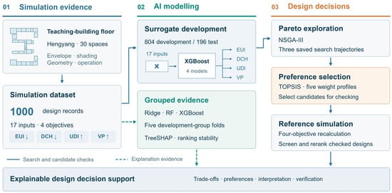
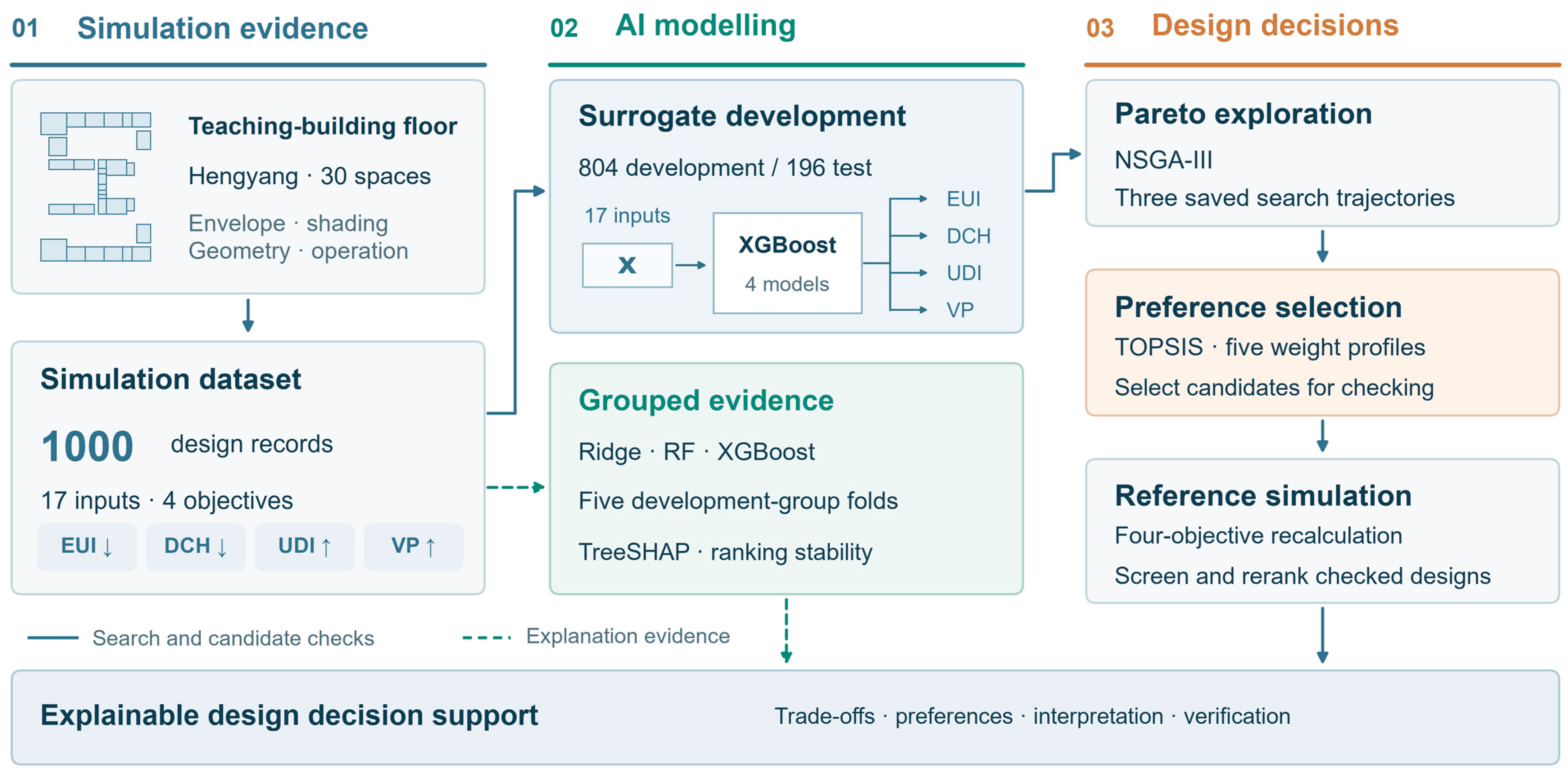
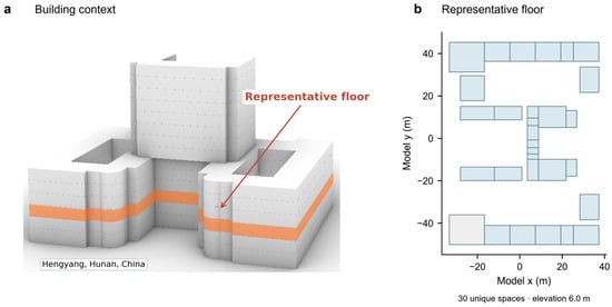
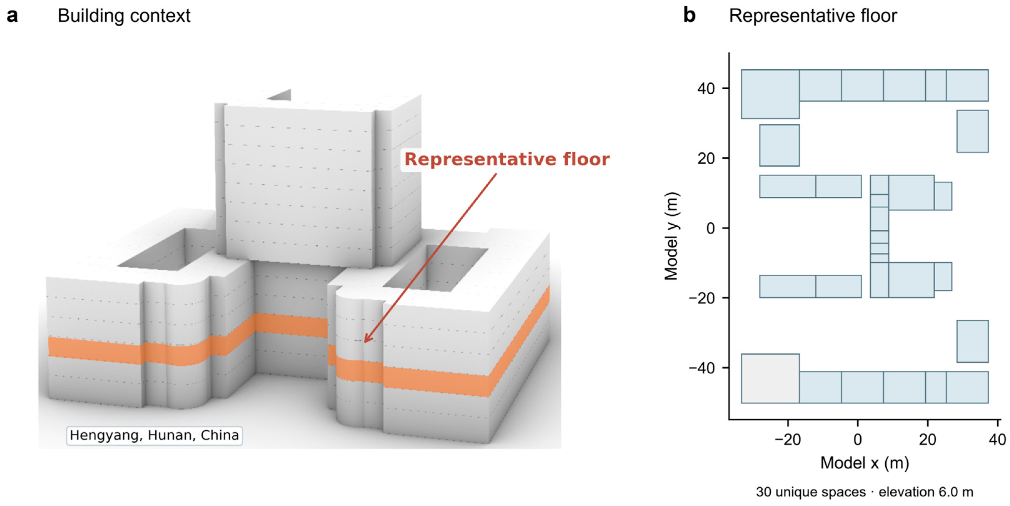
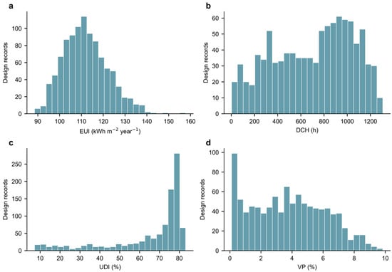
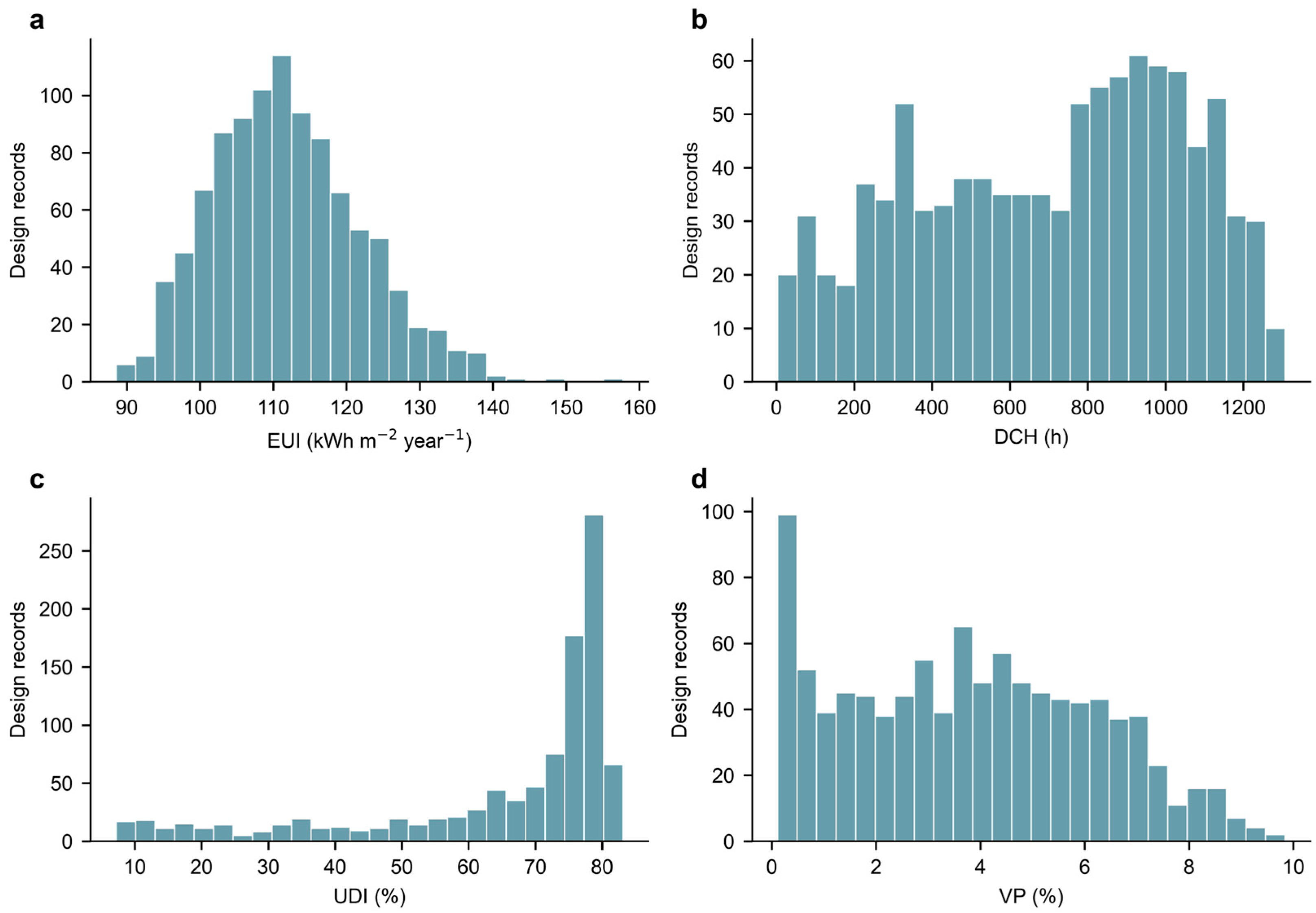
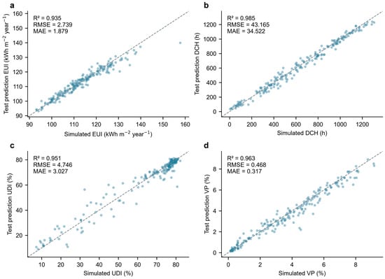
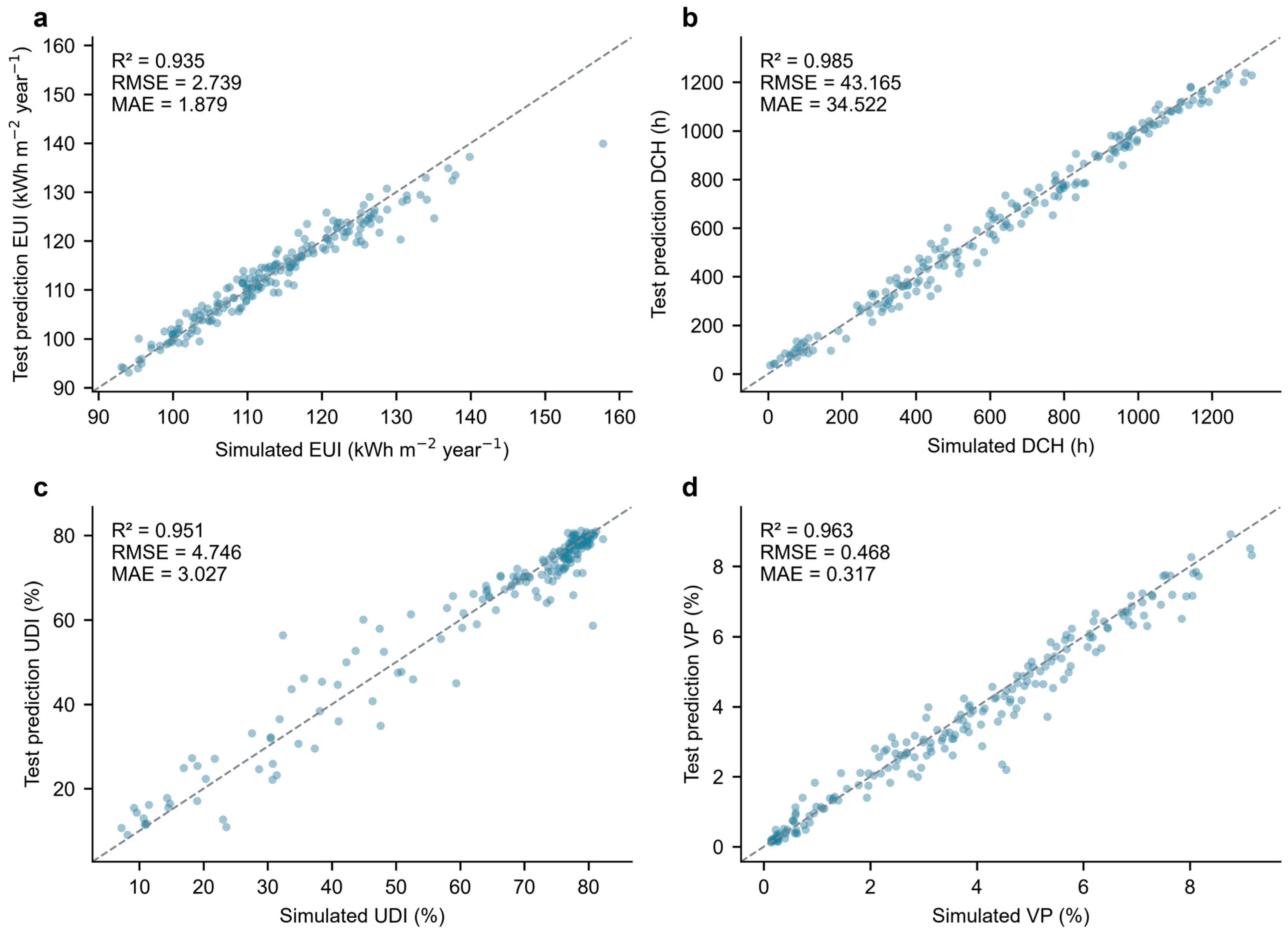
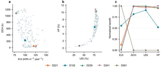
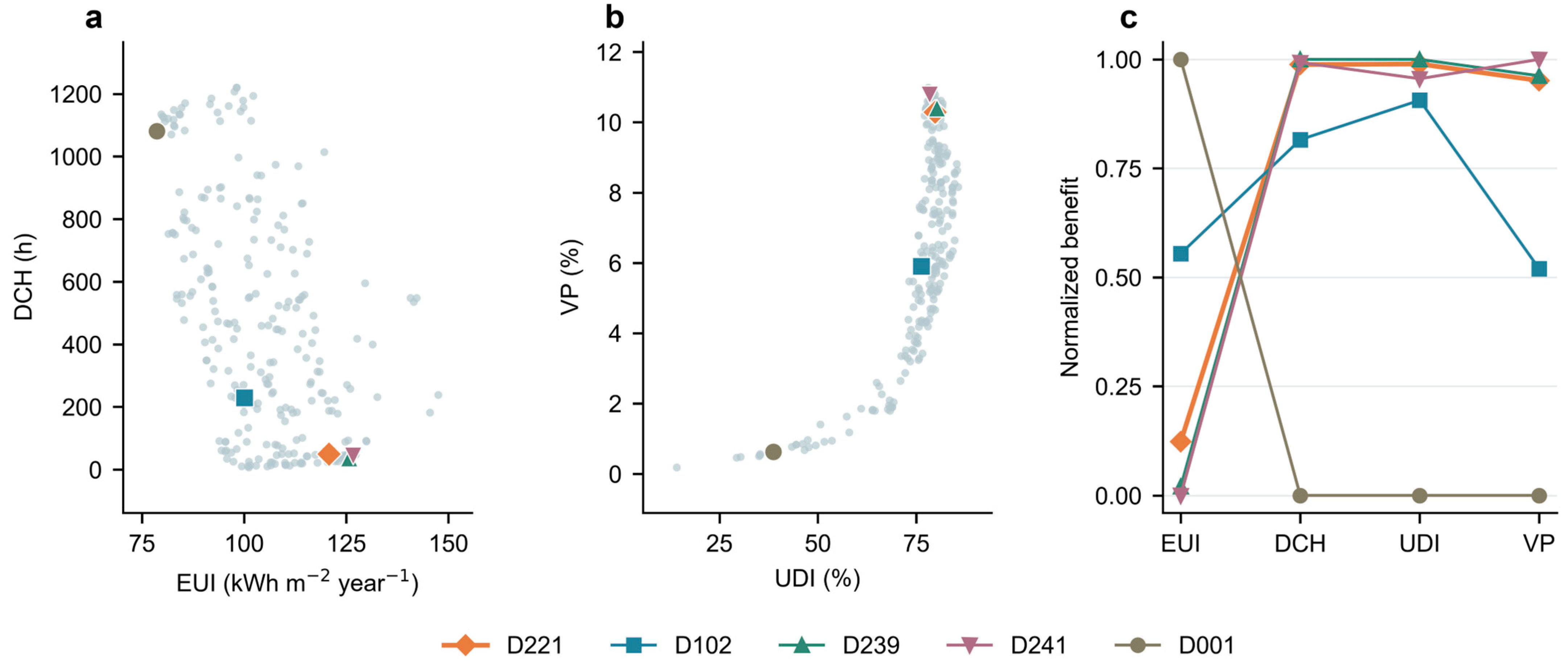
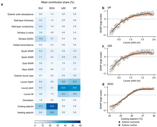
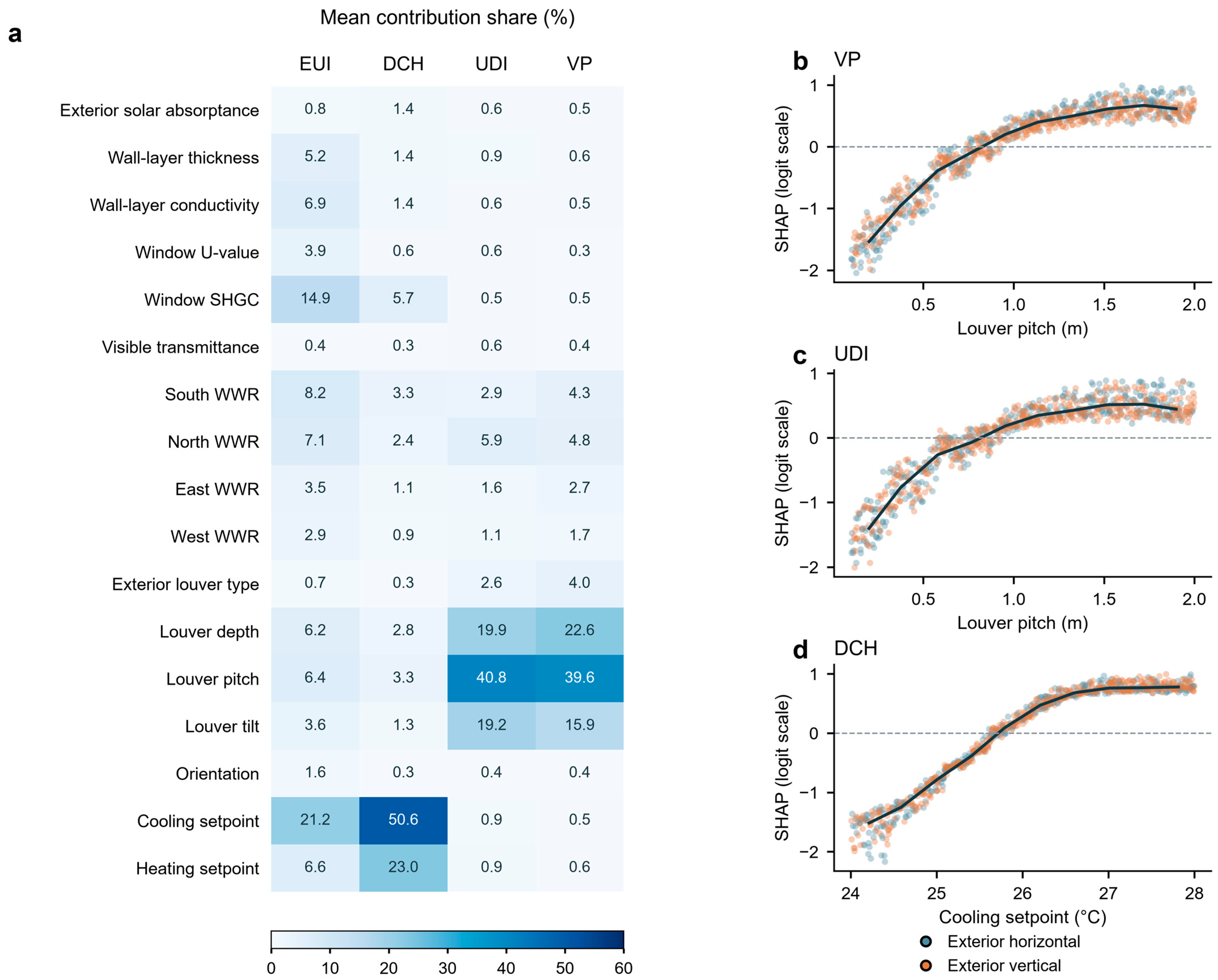
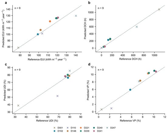
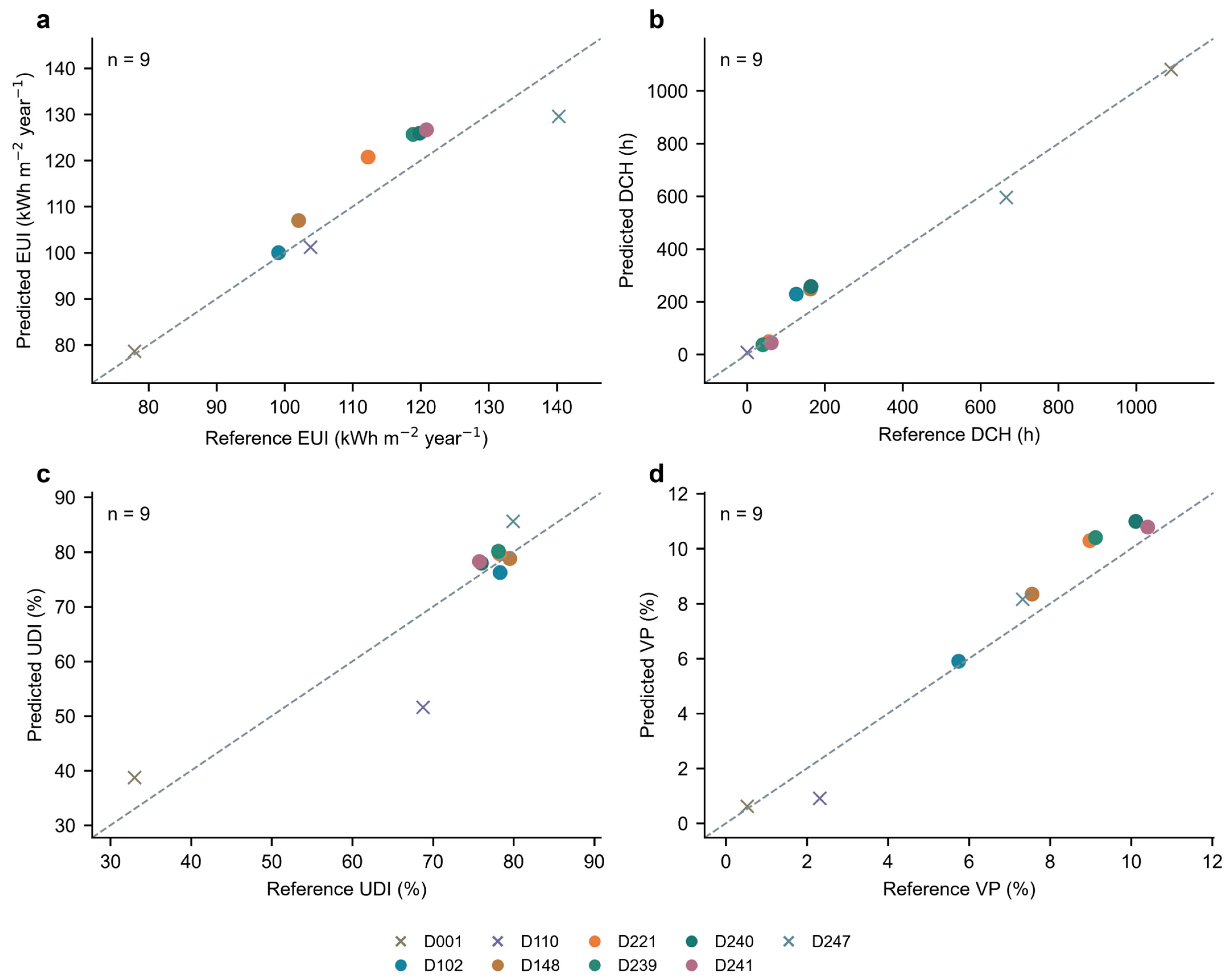
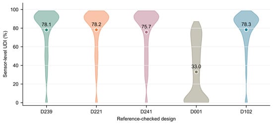
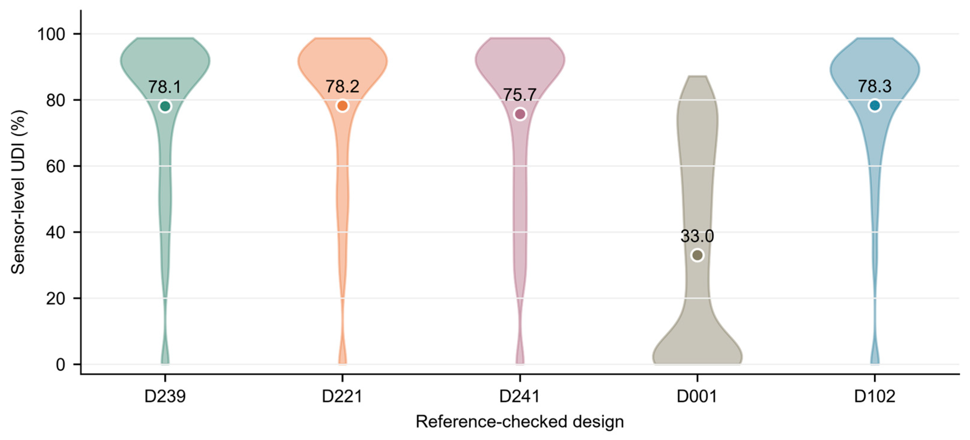
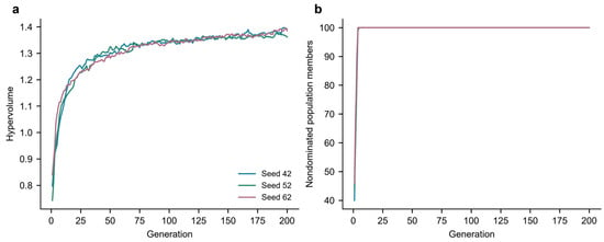
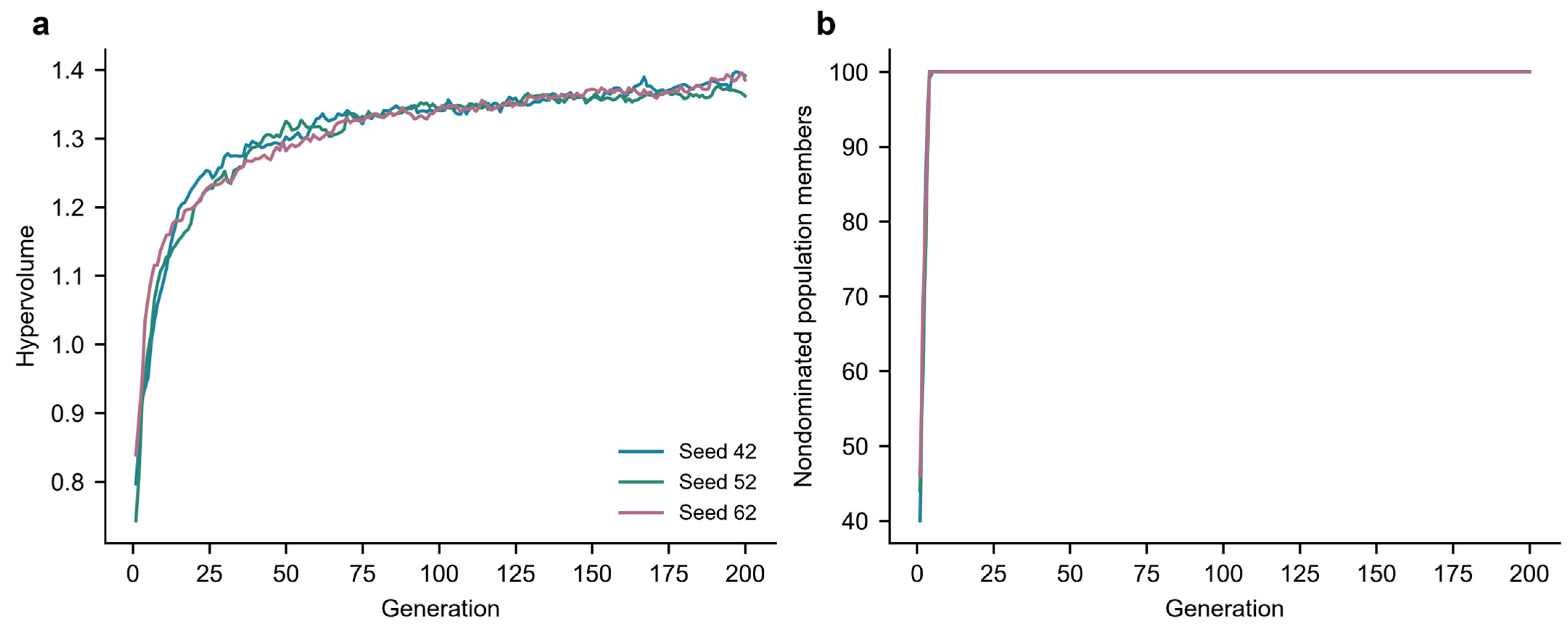

Disclaimer/Publisher’s Note: The statements, opinions and data contained in all publications are solely those of the individual author(s) and contributor(s) and not of MDPI and/or the editor(s). MDPI and/or the editor(s) disclaim responsibility for any injury to people or property resulting from any ideas, methods, instructions or products referred to in the content. |
© 2026 by the authors. Licensee MDPI, Basel, Switzerland. This article is an open access article distributed under the terms and conditions of the Creative Commons Attribution (CC BY) license.