Operator-Adapted Modal Spaces for Reduced-Order Forward Modeling and Parameter Inversion in Layered Consolidation

Abstract

Identifying the consolidation state of building foundations forms part of structural health monitoring and condition assessment of infrastructure in service. Recovering the coefficient of consolidation of each layer from pore water pressure monitoring requires repeated solution of the layered consolidation equation during a parameter search. The forward space is therefore required to remain fixed over the entire inversion and to be adapted to the flux condition at material interfaces; classical layered eigenbases and the global sine space each satisfy only one. This study constructs two operator-adapted modal spaces that satisfy both. The permeability operator basis is generated by an unweighted eigenvalue problem for the permeability operator, whereas the frozen storage basis solves a generalized eigenvalue problem with a storage weight proportional to the vertical permeability. Both depend only on the known layer positions and the relative permeability profile, not on its absolute magnitude. Under a unified projection, propagation, and full-order finite element reference, the three spaces are compared in a high-contrast four-layer configuration. Among the tested dimensions, the operator-adapted spaces first reach a full-period relative error of 10⁻² at 20 modes and the global sine space at 80. After the initial layer t < 10⁻³, the errors of the operator-adapted spaces decrease approximately as K^−2.1 to K^−4.1, compared with about K⁻¹ for the sine space, and neither operator-adapted basis is uniformly more accurate than the other. In a fixed four-layer geometry, the reduced-order gain increases with the permeability contrast. Within the same operator-adapted space, direct matrix propagation combined with bounded least squares yields lower parameter and field errors than a neural parameterization of the time coefficients. These results provide a quantitative basis for offline space construction and online solver selection in parameter identification for foundation consolidation monitoring.

1. Introduction

Assessment of the service performance of buildings and civil infrastructure depends on continuous knowledge of the state of the supporting ground. In saturated fine-grained soils, the dissipation of excess pore water pressure (EPWP) governs the rate at which settlement develops, and the coefficient of consolidation c_v of each layer determines the corresponding time scale [1,2]. Laboratory testing is the primary means of obtaining c_v, but sample disturbance, stress history, drainage conditions, and the interpretation method all affect the measured values [2]. Piezometers and settlement monitoring record directly how the ground evolves under construction and service loading. Recovering the layered c_v from these observations constitutes a ground state identification task within a structural health monitoring framework and supplies updated parameters for settlement prediction and maintenance decisions [3,4].

The computational structure of the inversion determines the choice of forward model. A parameter search requires the layered consolidation equation to be solved repeatedly over candidate values of c_v, so the efficiency and accuracy of a single solve are amplified by a factor of tens to hundreds. When a reduced-order forward model is adopted, this process involves two design decisions: which space representation is selected in the offline stage, and which solver and parameter estimation algorithm is adopted in the online stage. The two require separate assessment, since the relative merit of a space representation does not determine the choice of the online algorithm.

The two requirements on the offline space follow from the problem itself. First, the basis functions should be constructed before the inversion begins and should remain unchanged throughout the parameter search; a basis that depends on the parameters to be identified has to be rebuilt whenever a candidate value is updated. Second, the basis functions should be adapted to the material interfaces. In stratified ground, k_v jumps along depth, so the EPWP is continuous across an interface while, wherever the seepage flux is nonzero, its derivative jumps in inverse proportion to the adjacent permeabilities. A finite combination of functions that are smooth across the interface satisfies the flux balance there only where its derivative vanishes and cannot represent a nonzero flux derivative jump. The approximation efficiency is limited accordingly. The two existing classes of space each meet one of these requirements. Schiffman and Stein derived a general solution for one-dimensional layered consolidation [5], and Lee et al. showed that permeability and volume compressibility cannot always be replaced by a single coefficient of consolidation [6]. Subsequent analytical and semi-analytical studies have treated partial drainage, non-Darcy flow, continuous drainage, and multi-stage loading [7,8,9]. Classical eigenbases of this type carry the derivative jump at the interfaces naturally, but their self-adjoint weight function S = k_v/c_v contains the unknown c_v and must be rebuilt for each candidate parameter set during inversion. Walker et al. employed a global sine expansion to represent multilayered soil consolidation in a unified manner [10,11], and extended it to varied loading and impeded drainage [12]. The sine space does not change with the material parameters, and its smooth modes do not reflect the flux balance at permeability jumps. Spectral bases built from a fixed reference operator have been developed systematically as parameter-independent reduced-order spaces in reduced basis methods for parametrized partial differential equations and in multiscale finite element methods [13,14,15], whereas their use for parameter identification in layered consolidation remains limited.

The choice of online solver relates directly to recent data-driven methods. Physics-informed neural networks (PINNs) write the governing equation, the boundary conditions, and the observations into a single training objective, which provides a unified framework for forward and inverse problems governed by partial differential equations (PDEs) [16,17]; equation stiffness and gradient imbalance among the loss terms make such training difficult [18]. For heterogeneous and interface problems, mixed formulations, subdomain coupling, and operator eigenfunction encoding have been adopted to improve the spatial representation and the interface treatment [19,20,21]. In consolidation analysis, PINNs have been applied to two-dimensional pore pressure prediction, inversion of material and boundary parameters, scale transformation, and fusion of simulated and field data [22,23,24,25], as well as to prediction of stratified ground driven by short-term pore pressure records and to back-analysis of field settlement [3,4]. Recent work further covers large-deformation consolidation, time-dependent drainage, multi-stage surcharge loading, three-dimensional surrogates, physics-regularized regression, data assimilation under spatial variability, and long-term graph-recurrent prediction [26,27,28,29,30,31,32,33]. When the reduced-order dynamics are linear and few parameters are to be identified, the performance of a neural time parameterization relative to direct matrix propagation with bounded least squares has not been compared directly within the same space and under the same observations.

This study addresses the two decision points above. In the offline stage, two operator-adapted modal spaces that meet both requirements are constructed by replacing the unknown storage weight with two c_v-independent surrogates. The projection follows established spectral Galerkin practice; the contribution lies in the choice of these weights for inversion and in the quantitative comparison that follows. The permeability operator basis solves an unweighted eigenvalue problem, and the frozen storage basis solves the corresponding generalized eigenvalue problem with a storage weight proportional to k_v. Both are determined by the known layer positions and the relative k_v profile, and a common scaling of k_v leaves their eigenfunctions unchanged. Two reduced-order systems are derived from the weak form, the operator-matched construction is verified under the proportional condition, and the three spaces are compared against the Walker-type sine space under a unified projection, propagation, and full-order finite element reference. In the online stage, the same permeability operator space is retained, and direct matrix propagation with bounded least squares is compared with a neural parameterization of the time coefficients in terms of inversion performance. The classical inversion is also repeated with all three spaces and with the classical eigenbasis rebuilt for each candidate, to quantify the accuracy and cost of fixing the space.

2. Problem Formulation

2.1. Layered Consolidation Equation

A saturated soil column of thickness H is considered. Known interfaces Z = Z₁, …, Z_L−1 divide the column into L horizontal soil layers. The physical depth coordinate is Z[m], and layer 𝓁 occupies ${\Omega }_{\mathcal{l}}^{*}=\left(Z_{\mathcal{l}-1},Z_{\mathcal{l}}\right)$, with Z⁰ = 0 and Z_L = H. The excess pore water pressure is denoted by U(Z,T) [Pa] and time by T [s]. Within each layer, the vertical permeability $k_{v,\mathcal{l}}^{*}\left[\mathrm{m}{\mathrm{s}}^{-1}\right]$, the coefficient of consolidation $c_{v,\mathcal{l}}^{*}\left[{\mathrm{m}}^2{\mathrm{s}}^{-1}\right]$, and the coefficient of volume compressibility $m_{v,\mathcal{l}}^{*}\left[\mathrm{P}{\mathrm{a}}^{-1}\right]$ are taken as positive constants. The unit weight of water is γ_w [Nm⁻³].

The material coefficients satisfy Equation (1):

$$c_v^{*}={\displaystyle \frac{k_v^{*}}{m_v^{*}{\gamma }_w}},S^{*}={\displaystyle \frac{k_v^{*}}{c_v^{*}}}=m_v^{*}{\gamma }_w$$

(1)

in which S^* [m⁻¹] denotes the storage coefficient used in the self-adjoint form. When the material properties do not vary with time and no source term is present after loading is complete, the governing equation is given by Equation (2).

$$S^{*}\left(Z\right){\displaystyle \frac{\partial U}{\partial T}}-{\displaystyle \frac{\partial }{\partial Z}}\left(k_v^{*}\left(Z\right){\displaystyle \frac{\partial U}{\partial Z}}\right)=0$$

(2)

This form distinguishes the respective roles of permeability and compressibility.

2.2. Nondimensionalization and Assumptions

Let z = Z/H, t = T/T⁰, and u = U/U⁰, where T⁰ and U⁰ denote the characteristic time and the initial pressure, respectively. With $k_v^{*}=k_{v0}{k}_v$ and $c_v^{*}=c_{v0}{c}_v$, and with the storage coefficient scaled by k_v0/c_v0, Equation (2) reduces to Equation (3).

$$S\left(z\right){\displaystyle \frac{\partial u}{\partial t}}-C_F{\displaystyle \frac{\partial }{\partial z}}\left(k_v\left(z\right){\displaystyle \frac{\partial u}{\partial z}}\right)=0,S\left(z\right)={\displaystyle \frac{k_v\left(z\right)}{c_v\left(z\right)}},C_F={\displaystyle \frac{c_{v0}{T}_0}{H^2}}$$

(3)

Variables and coefficients written without an asterisk are dimensionless.

The fixed numerical setting adopted throughout uses 0 < z < 1 and 0 ≤ t ≤ 1, takes U⁰ as the pressure scale, and sets C_F = 1.2. For a fixed dimensionless material profile, changing the positive constant C_F only rescales the dimensionless time coordinate. This value therefore does not affect any of the comparisons reported below, provided that it is held consistent across all cases. All subsequent equations are written in this dimensionless system. As an example, a soil column of thickness H = 5 m under a surcharge of 80 kPa, monitored for two years, gives U⁰ = 80 kPa and T⁰ = 2 years, and C_F = 1.2 then corresponds to c_v0 = 15 m²/year. The dimensionless values c_v = 0.05–0.6 used in the examples below correspond to 0.7–9 m²/year, and a dimensionless time interval of 0.01 corresponds to about one week.

The model is linear. The layer interfaces are known and fixed, and c_v(z) in each layer is the quantity to be identified.

For any test function $v\in H_0^1\left(0,1\right)$, multiplying Equation (3) by v, integrating by parts within each layer, and applying the flux continuity condition at the interfaces given in Equation (6) yields Equation (4).

$${\int }_0^1\mathit{Sv}{u}_t\mathrm{d}z+C_F{\int }_0^1{k}_v{v}^{\prime }{u}^{\prime }\mathrm{d}z=0$$

(4)

This weak form separates the storage coefficient S = k_v/c_v from the permeability operator. Both reduced-order systems and the independently assembled full-order finite element reference model are constructed from this form.

2.3. Boundary, Interface, and Initial Conditions

Both ends of the dimensionless soil column are drainage boundaries:

u(0,t) = u(1,t) = 0, t > 0.

(5)

At each interface z = z_𝓁, the excess pore water pressure and the vertical seepage flux are continuous:

$$⟦u{⟧}_{z_{\mathcal{l}}}=0,⟦k_v{u}_z{⟧}_{z_{\mathcal{l}}}=0, \mathcal{l}=1,\dots ,L-1$$

(6)

Here ⟦·⟧ denotes the right-hand limit minus the left-hand limit. These are the classical pressure and flux conditions for layered consolidation systems [5]. In the finite element implementation, Equation (6) is satisfied in the variational sense through a conforming weak space, whereas the one-sided flux recovered from a piecewise linear field depends on the mesh and on the derivative recovery procedure.

The initial condition adopted in all cases is

u(z,0) = 1 for almost every z ∈ (0, 1)

(7)

The uniform interior initial value is incompatible with the instantaneous drainage values at the end points. This discontinuity affects only the end points under a continuous L² projection, and it excites high-frequency components in an undamped time discretization. The reduced-order models therefore apply a consistent mass projection to Equation (7), while the full-order reference model uses the start-up smoothing described in Section 4.1.

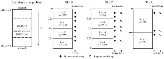
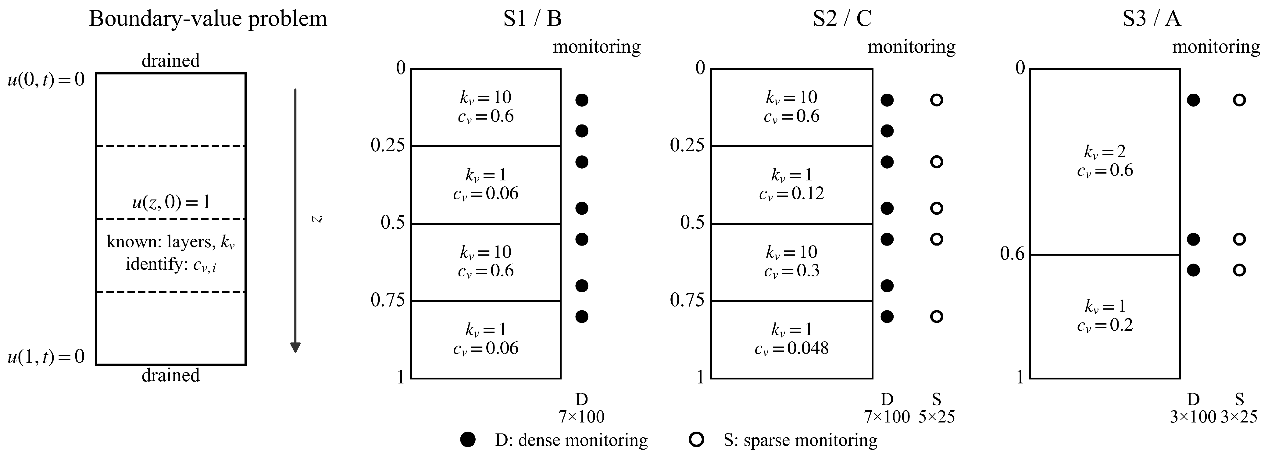
The boundary value problem, the material profiles, and the observation layouts are summarized in Figure 1.

Figure 1. Layered consolidation problem and observation layouts.

Among the three material configurations, S1 and S2 both have four layers with interfaces at z = 0.25, 0.50, and 0.75, and share the same relative profile k_v = [10, 1, 10, 1], differing only in the values of c_v of each layer. The two operator-adapted spaces can therefore be reused directly between S1 and S2 without reconstruction. S3 has two layers with a single interface at z = 0.6, and the material contrast is reduced from 10 to 2. The observation layouts are labeled as “number of sensors × number of observation times”: S1 uses a dense layout of 7 × 100; the sparse layout of S2 reduces the sensors to 5 and the observation times to 25; the dense and sparse layouts of S3 use the same three sensor positions and reduce the observation times from 100 to 25.

3. Reduced-Order Formulation and Online Solvers

3.1. Global Sine Galerkin Reference Space

The Walker-type global sine Galerkin expansion provides a material-independent reference space for the three-basis comparison. For a truncation dimension K, the orthonormal basis is

$${\chi }_j\left(z\right)=\sqrt{2}\sin \left(\mathit{j\pi z}\right),j=1,\dots ,K$$

(8)

with $u_K\left(z,t\right)={\sum }_{j=1}^K{\chi }_j\left(z\right)a_j\left(t\right)$. The factor $\sqrt{2}$ gives unit norm in L²(0, 1), and the unnormalized sine functions used by Walker span the same truncated space. The doubly drained wavenumbers and the layered matrix assembly follow the spectral Galerkin construction of [10,11]. A positive stiffness notation is adopted throughout.

Substituting into Equation (4) gives

$${\Gamma }_{\mathit{ij}}={\sum }_{\mathcal{l}=1}^L{\int }_{{\Omega }_{\mathcal{l}}}{\displaystyle \frac{k_{v,\mathcal{l}}}{c_{v,\mathcal{l}}}}{\chi }_i{\chi }_j\mathrm{d}z$$

(9)

$${\mathsf{\Theta }}_{\mathit{ij}}={\sum }_{\mathcal{l}=1}^L{\int }_{{\Omega }_{\mathcal{l}}}{k}_{v,\mathcal{l}}{\chi }_i^{\prime }{\chi }_j^{\prime }\mathrm{d}z$$

(10)

$$\Gamma \dot{\dot{\mathbf{a}}}+C_F\mathsf{\Theta }\mathbf{a}=0$$

(11)

When the material parameters of all layers are positive and the modes are linearly independent, Γ,Θ ∈ ℝ ^K×K are symmetric positive definite. All integrals are evaluated separately within each material layer. The implementation uses analytical integration of the sine products, with layered Gauss–Legendre quadrature as an independent algebraic verification.

3.2. Permeability Operator Basis

Beyond the sine reference space, the known permeability profile can be used directly to generate operator-adapted modes:

$$-{\displaystyle \frac{\mathrm{d}}{\mathrm{d}z}}\left(k_v\left(z\right){\displaystyle \frac{\mathrm{d}{\varphi }_j}{\mathrm{d}z}}\right)={\lambda }_j{\varphi }_j,{\varphi }_j\left(0\right)={\varphi }_j\left(1\right)=0$$

(12)

These modes are continuous, satisfy the weak interface balance of $k_v{\varphi }_j^{\prime }$, and are normalized according to

$${\int }_0^1{\varphi }_i{\varphi }_j\mathrm{d}z={\delta }_{\mathit{ij}}$$

(13)

In an interface-conforming piecewise linear (P1) finite element space, Equations (12) and (13) are obtained from

K_vΦ = M₀ΦΛ, Φ^𝖳M₀Φ = I, Φ^𝖳K_vΦ = Λ

(14)

where K_v and M⁰ denote the permeability stiffness matrix and the unweighted consistent mass matrix, respectively. The diagonal matrix Λ = diag(λ₁, …, λ_K) is positive definite. With the layer positions, the relative k_v profile, and the mesh held fixed, this trial space is independent of the unknown c_v.

The layer Gram matrices are defined as

$$G_{\mathcal{l},\mathit{ij}}={\int }_{{\Omega }_{\mathcal{l}}}{\varphi }_i{\varphi }_j\mathrm{d}z,G_{\mathcal{l}}\in {\mathbb{R}}^{K\times K}$$

(15)

and the modal mass matrix as

$$B^{\left(P\right)}\left(c_v\right)={\sum }_{\mathcal{l}=1}^L{\displaystyle \frac{k_{v,\mathcal{l}}}{c_{v,\mathcal{l}}}}{G}_{\mathcal{l}}$$

(16)

Each G_𝓁 is symmetric positive semidefinite. Equation (16) shows that B^(P) is affine in 1/c_v,𝓁: the layer Gram matrices G_𝓁 are computed once in the offline stage, after which each candidate c_v requires only O(LK²) operations to assemble the reduced-order mass matrix, without returning to the full-order mesh. This affine structure is the computational basis of the offline stage and online stage decomposition in the parameter search. For c_v,𝓁 > 0, B^(P)(c_v) is symmetric positive definite. Expanding $u_K={\sum }_{j=1}^K{\varphi }_j{a}_j$ gives

$$B^{\left(P\right)}\left(c_v\right)\dot{\mathbf{a}}+C_F\Lambda \mathbf{a}=0$$

(17)

In Equation (12), k_v appears only inside the differential operator and the right-hand side is an unweighted mass form. These modes are referred to below as the permeability operator basis. A common scaling of the permeability gives

$$-\left(\right(\alpha k_v){\varphi }_j^{\prime }{)}^{\prime }=\alpha {\lambda }_j{\varphi }_j,\alpha >0$$

(18)

The eigenfunctions and the trial space they span are therefore unchanged, while the eigenvalues scale as λ_j ↦ αλ_j.

3.3. Frozen-Storage Basis

The true consolidation eigenvalue problem is −${\left(k_v{q}^{\prime }\right)}^{\prime }=\mathit{\omega Sq}$, whose weight function S = k_v/c_v = m_vγw contains the parameters to be identified. Each of the two operator-adapted constructions replaces this weight function by a surrogate that is independent of c_v. Equation (12) takes the weight as a constant, which corresponds to m_v being uniform with depth, whereas the construction of this section takes the weight proportional to k_v, which corresponds to c_v being uniform with depth. The latter retains the material-dependent mass weighting and fixes it at a prior reference value c_v,ref before the comparison:

$$-{\displaystyle \frac{\mathrm{d}}{\mathrm{d}z}}\left(k_v\left(z\right){\displaystyle \frac{\mathrm{d}{\psi }_j}{\mathrm{d}z}}\right)={\mu }_j{S}_{\mathrm{ref}}\left(z\right){\psi }_j,S_{\mathrm{ref}}\left(z\right)={\displaystyle \frac{k_v\left(z\right)}{c_{v,\mathrm{ref}}}},{\psi }_j\left(0\right)={\psi }_j\left(1\right)=0$$

(19)

The reference value is taken as the same scalar in all layers; here, the midpoint of the inversion bounds on a logarithmic scale, c_v,ref = 0.1414. As shown at the end of this section, this value does not change the trial space. The modes are normalized under the frozen storage inner product:

$${\int }_0^1{S}_{\mathrm{ref}}{\psi }_i{\psi }_j\mathrm{d}z={\delta }_{\mathit{ij}}$$

(20)

The discrete generalized eigenvalue problem is

K_vΨ = M_refΨ$ℳ$, Ψ^𝖳M_refΨ = I, Ψ^𝖳K_vΨ = $ℳ$

(21)

where M_ref is assembled from S_ref and $ℳ$ = diag(μ₁, …, μ_K). For a candidate c_v, the modal mass matrix is defined as

$$B_{\mathit{ij}}^{\left(F\right)}\left(c_v\right)={\sum }_{\mathcal{l}=1}^L{\int }_{{\Omega }_{\mathcal{l}}}{\displaystyle \frac{k_{v,\mathcal{l}}}{c_{v,\mathcal{l}}}}{\psi }_i{\psi }_j\mathrm{d}z$$

(22)

The reduced-order dynamical system in the frozen storage space is

$$B^{\left(F\right)}\left(c_v\right)\dot{\mathbf{b}}+C_F\mathcal{M}\mathbf{b}=\mathbf{0}$$

(23)

Since c_v,ref takes the same scalar value in all layers, S_ref is proportional to k_v, and Equation (19) reduces to $-{\left(k_v{\psi }_j^{\prime }\right)}^{\prime }={\nu }_j{k}_v{\psi }_j$ with ν_j = μ_j/c_v,ref. The trial space therefore does not contain c_v,ref, and changing this reference value only scales the eigenvalues. The difference between the two operator-adapted constructions thus reduces to the weight function of the mass term, which is unity in Equation (12) and k_v in Equation (19). Under a common scaling k_v ↦ αk_v, both K_v and M_ref are multiplied by α, and the eigenfunctions and ν_j remain unchanged. Normalization changes the scale of an individual eigenfunction but not the trial space. Both constructions therefore depend only on the layer positions and the relative k_v profile.

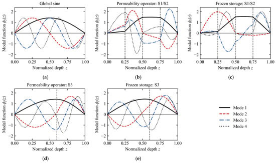
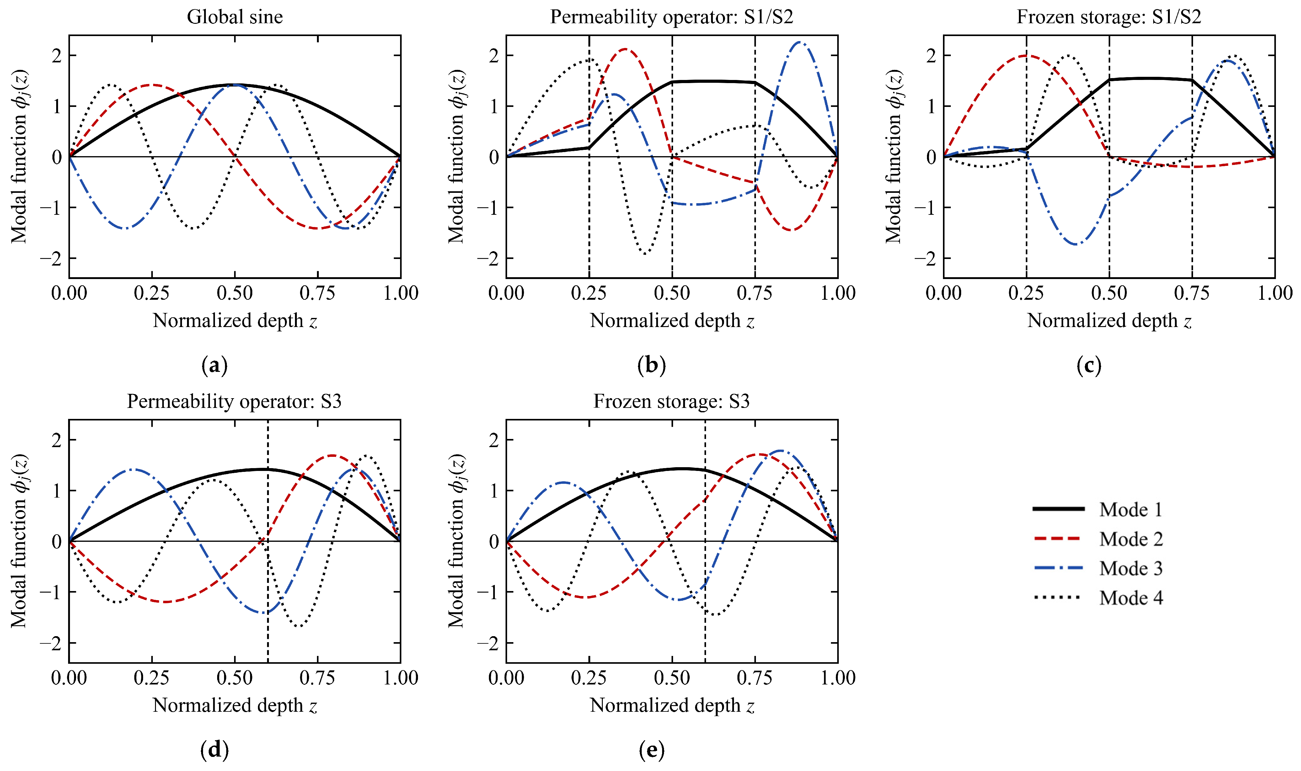
The first four functions of the global sine space and of the two operator-adapted constructions are shown in Figure 2.

Figure 2. First four modes of the three trial spaces. (a) Global sine space; (b) permeability operator for S1/S2; (c) frozen storage spaces for S1/S2; (d) permeability operator for S3; (e) frozen storage spaces for S3.

Both operator-adapted families exhibit a slope break at every interface, marked by the vertical dashed lines. The gradient is steep within the low-permeability layers and nearly flat within the high-permeability layers. For the continuous eigenfunctions, the slope ratio across an interface equals the reciprocal of the permeability ratio, so that k_vφ′ is continuous; the P1 modes satisfy this condition only through the discrete variational equations. The one-sided fluxes recovered from the adjacent elements measure the remaining discrepancy. Their relative jump, $\left|{k_v}^{-}{\phi }^{\prime -}-{k_v}^{+}{\phi }^{\prime +}\right|/\left[\left(\left|{k_v}^{-}{\phi }^{\prime -}\right|+\left|{k_v}^{+}{\phi }^{\prime +}\right|\right)/2\right]$, is at most 4.7 × 10⁻² for the first four modes of both families on the 3201-node mesh, and every value above round-off halves on the 6401-node mesh. For the global sine modes, which are smooth across the interfaces, the same measure equals $2\left|{k_v}^{-}-{k_v}^{+}\right|/\left({k_v}^{-}+{k_v}^{+}\right)$ on both meshes, namely, 1.64 in S1/S2 and 0.67 in S3. Interfaces at which the flux of a mode vanishes are excluded from the measure. A finite sine combination therefore satisfies flux continuity only where its derivative vanishes and cannot represent the derivative jump that accompanies a nonzero flux. The mode shapes of the two operator-adapted constructions are close to each other, and the difference lies mainly in how the higher modes distribute their amplitude among the layers. The material contrast of S3 is lower (Figure 2d,e), and the differences in mode shape among the three spaces are correspondingly smaller.

3.4. Verification of the Operator-Matched Construction in the Proportional Case

The storage coefficient of the entire soil column is assumed to be constant:

$${\displaystyle \frac{k_v\left(z\right)}{c_v\left(z\right)}}=s>0$$

(24)

For the permeability operator basis, Equations (13), (15) and (16) give

$$B_{\mathit{ij}}^{\left(P\right)}=s{\int }_0^1{\varphi }_i{\varphi }_j\mathrm{d}z=s{\delta }_{\mathit{ij}},B^{\left(P\right)}=\mathit{sI}$$

(25)

Equation (17) therefore decouples into

$$s{\dot{a}}_j+C_F{\lambda }_j{a}_j=0,a_j\left(t\right)=a_j\left(0\right)\exp \left(-{\displaystyle \frac{C_F{\lambda }_j}{s}}t\right)$$

(26)

The same condition also makes φ_j an exact continuous eigenfunction of the consolidation operator: the physical generalized eigenvalue problem $-{\left(k_v{q}^{\prime }\right)}^{\prime }=\mathit{\omega Sq}$ reduces to Equation (12), with ω_j = λ_j/s. Configuration S1 is used to verify this operator-matching identity and its numerical implementation. In the continuous formulation and in the permeability operator coordinates, the spatial approximation error arises from the finite truncation of the exact spectrum at K.

3.5. Initial Projection

The main analysis uses the same unweighted consistent L² projection for all three spaces. If V = (v₁, …, v_K) denotes the selected basis, the initial coefficients are obtained from

$$M_0^r{\mathbf{a}}_0={\mathbf{b}}_0,(M_0^r{)}_{\mathit{ij}}={\int }_0^1{v}_i{v}_j\mathrm{d}z,({\mathit{b}}_0{)}_i={\int }_0^1{v}_i{u}_0\mathrm{d}z$$

(27)

The main results use this unweighted projection. In the sensitivity analysis, both integrals are replaced by the corresponding S-weighted integrals, and the same rule is applied to all bases.

For the neural coefficient model, the projected coefficients are imposed through

a_θ(t) = a₀ + β(t)N_θ(t), β(0) = 0

(28)

The condition a_θ(0) = a₀ is therefore satisfied exactly in the coefficient space, without an initial condition penalty term.

3.6. Classical Reduced-Order Propagation and Inversion

Each reduced-order system can be written as

$$M_r\dot{\mathbf{a}}+C_F{K}_r\mathbf{a}=0$$

(29)

For a symmetric positive definite matrix pair, the implementation solves

K_rQ = M_rQΞ, Q^𝖳M_rQ = I

(30)

and propagates according to

a(t) = Qexp(−C_FΞt)Q^𝖳M_ra₀

(31)

The inverse of M_r is not formed explicitly. Apart from floating point eigensolution error, Equation (31) gives the solution of the matrix ordinary differential equation within the selected truncated space.

The inversion tests use the permeability operator basis, assembled once from the fixed k_v profile and the layer positions. The online solvers are compared at K = 10; the dependence of the classical estimates on K and on the choice of space is examined in Section 5.3. At K = 10, the classical inversion observes u_K(z_p,t_n;c_v) = ϕ(z_p)^Ta(t_n;c_v) and solves

$${\min }_{\mathbf{q}}{\displaystyle \frac{1}{2}}{\sum }_{p,n}{\left[{\displaystyle \frac{u_K\left(z_p,t_n;\exp \mathbf{q}\right)-d_{\mathit{pn}}}{U_{\mathrm{scale}}}}\right]}^2,\log \left(0.02\right)\le q_{\mathcal{l}}\le \log \left(1.0\right)$$

(32)

where the observations d_pn, like u_K, are expressed in the dimensionless system of Section 2.2, i.e., normalized by U⁰, and U_scale is a dimensionless observation scale, taken here as 1. This constant does not vary with the parameters, so it changes only the absolute magnitude of the objective function and not the location of the minimizer. The data d_pn are generated by an independently assembled full-order finite element model on a 1601-node interface-conforming mesh, using backward Euler time integration with Δt = 1/6400 from the uniform initial vector on the free nodes; the sensor values are obtained by linear interpolation of the nodal field. Matrix propagation combined with bounded least squares constitutes the main online inversion solver, and every identified parameter vector is recomputed with the full-order model.

3.7. Neural Coefficient Parameterization

The alternative online solver uses a fully connected tanh network that maps dimensionless time to K modal coefficients. With a = S_aâ, the unscaled weak modal residual is

$$\mathbf{r}\left(t\right)=B^{\left(P\right)}\left(c_v\right)S_a{\displaystyle \frac{\mathrm{d}\mathit{â}}{\mathrm{d}t}}+C_F\Lambda S_a\mathit{â}$$

(33)

The residual preconditioner is fixed before optimization. With T_char = 1 and B_ref = B^(P)(c_v,ref), the row scaling is

$$D_i={[{\sum }_j{\left({\displaystyle \frac{(B_{\mathrm{ref}}{)}_{\mathit{ij}}{S}_{a,j}}{T_{\mathrm{char}}}}\right)}^2+(C_F{\lambda }_i{S}_{a,i}{)}^2]}^{1/2}$$

(34)

The values D_i are held constant during training and are constructed from the midpoint of the prior bounds.

The network is a fully connected tanh architecture with four hidden layers of width 64, operating in float64, which maps scalar time to K = 10 modal coefficients. The spatial variation, including the slope breaks at the interfaces, is carried by the modal basis, and the network represents only the K modal coefficients, which are non-oscillatory functions of time; architectures designed for high-frequency content, such as Fourier-feature embeddings, were therefore not evaluated.The hard initial value is imposed through Equation (28) with β(t) = 1 − exp(−t/0.01), and the modal coefficients are normalized by S_a,j = max(|a_0,j|,0.05). The inversion loss is the weighted sum of the physics residual and the observation residual, with weights of 1 and 100, respectively; neither dynamic weighting nor alternating updates are used. Training was carried out first with Adam for 4000 steps, with 256 collocation points resampled at each step and a learning rate of 2 × 10⁻³ decayed once at step 2500 and once at step 3500. L-BFGS was then applied for at most 2000 iterations on a fixed set of 401 collocation points, using a strong Wolfe line search. Three random seeds (11, 22, and 33) were combined with two bounded initial values, giving six runs for each configuration. The neural runs were executed in float64 on an NVIDIA RTX 3060 Laptop GPU, and the classical runs used LAPACK in float64 on the Intel Core i7-11800H CPU (8 cores) of the same laptop with default library threading, under Windows with Python 3.10, NumPy 1.26, SciPy 1.15, and PyTorch 2.6 with CUDA 11.8.

Classical propagation and the neural time coefficient parameterization share the permeability operator space and the modal mass matrix B^(P)(c_v). The comparison between them therefore focuses on the time representation, the optimization process, the errors, and the computational cost.

4. Numerical Verification and Modal Space Comparison

4.1. Reference Solution and Its Numerical Verification

The reduced-order solutions are assessed against an independently assembled, interface-conforming P1 finite element model. The semi-discrete system is

$$M_S\dot{\mathbf{u}}+C_F{K}_v\mathbf{u}=\mathbf{0}$$

(35)

where M_S contains the layered coefficient S = k_v/c_v and K_v contains k_v. After the drainage end point degrees of freedom are eliminated, a uniform initial vector is imposed on the free nodes before time integration.

The reference solution uses 6401 nodes and a step size Δt = 1/6400 = 0.00015625 and retains all 6401 time levels over 0 ≤ t ≤ 1. To resolve the initial layer, the interval [0, 0.01] is recomputed with Δt/8 and [0, 0.001] with Δt/64, and these time levels are added to the error quadrature; the resulting time grid is denoted T3. Compared with the grid that omits the Δt/64 levels, T3 changes the error over t ≥ 0.001 by less than 10⁻⁴ in relative terms, apart from values of about 2 × 10⁻⁷ at the resolution of the modal discretization, and leaves the mode numbers at the 10⁻² threshold unchanged for every space and case. The full-period error at K ≥ 40 remains sensitive to the sampling of the initial layer and changes by up to 38% between these two grids, so its values at those dimensions are not used quantitatively. Time integration uses the Rannacher-smoothed Crank–Nicolson method, in which two backward Euler half steps are performed over the first time interval and Crank–Nicolson is used thereafter. The lowest observed temporal convergence order was 2.239 across all cases and over both the full period and the early window. The maximum difference between an independently implemented BDF2 scheme started with backward Euler and the reference at these output instants was 3.516 × 10⁻⁶.

The joint space–time error bounds for the three cases over the full period and the early window are summarized in Table 1. Each bound is an empirical estimate, formed as the sum of the relative changes of the solution under mesh refinement and under time-step refinement.

Table 1. Empirical numerical verification bounds for the full-order reference.

Case/Window	Global Bound	Global Limit	Interface Bound	Interface Limit
S1, full period	2.534 × 10−5	1.0 × 10−4	2.171 × 10−7	5.0 × 10−4
S1, 0 ≤ t ≤ 0.05	6.628 × 10−5	2.0 × 10−4	8.962 × 10−7	5.0 × 10−4
S2, full period	2.366 × 10−5	1.0 × 10−4	2.223 × 10−7	5.0 × 10−4
S2, 0 ≤ t ≤ 0.05	6.598 × 10−5	2.0 × 10−4	9.275 × 10−7	5.0 × 10−4
S3, full period	4.467 × 10−5	1.0 × 10−4	2.845 × 10−8	5.0 × 10−4
S3, 0 ≤ t ≤ 0.05	7.440 × 10−5	2.0 × 10−4	6.476 × 10−8	5.0 × 10−4

Note: The 6401-node Rannacher-smoothed Crank–Nicolson result is used as the reference throughout.

It is observed that the global error bound in all six rows is a factor of 2.2 to 4.2 below the corresponding limit, and the interface error bound is 2.7 to 4.2 orders of magnitude below its limit. The global error bound in the early window is about two to three times that over the full period, which indicates that the numerical error of the reference solution originates mainly from the strong gradients in the initial stage.

When the initial value and the boundary values are incompatible, the unsmoothed Crank–Nicolson scheme produced nodal pressures with a minimum of −0.9422. No corresponding substantial sign reversal occurred with either the Rannacher–Crank–Nicolson scheme or the BDF2 recursion. The subsequent comparisons therefore use the 6401-node finite element field, which passed both the spatial and the temporal convergence checks, as the unified reference.

Both the permeability operator basis and the frozen storage basis with K ≤ 80 are assembled on an interface-conforming 3201-node mesh. Their P1 modes are transferred element by element to the common 6401-node mesh by linear interpolation. The two meshes are nested, so the values at the original nodes remain unchanged and only the newly added intermediate nodes are interpolated, without smoothing or derivative recovery. For the permeability operator family, the maximum difference between the 3201-node and 6401-node reduced-order fields was 8.01 × 10⁻⁵ for S1 and S2 and 4.73 × 10⁻⁵ for S3. The frozen storage basis was verified on the same meshes, using layered exact integration and an independent 6401-node eigenpair check.

The maximum relative Frobenius difference between the analytical sine matrices and layered Gauss–Legendre integration at doubled order was 1.87 × 10⁻¹⁴. The difference between the symmetric generalized propagation and verification by the matrix exponential and by high-accuracy DOP853 integration did not exceed 1.809 × 10⁻¹¹, and the maximum residual of the projection normal equations was 5.407 × 10⁻¹⁶. For the newly added frozen storage basis, the largest generalized eigenvalue residual in the verification series was 2.45 × 10⁻¹³, and the maximum frozen mass orthogonality error was 5.87 × 10⁻¹⁵.

4.2. Comparison Cases and Error Metrics

The three cases used for the modal space comparison are given in Table 2. Each case also carries an inverse configuration label, A, B, or C, with two unknowns in A and four in B and C; these configurations are defined in Section 5.2.

Table 2. Cases used for the modal space comparison.

Case	Interfaces	Relative kv	cv	Inverse Configuration	Role
S1	0.25, 0.50, 0.75	10, 1, 10, 1	0.60, 0.06, 0.60, 0.06	B	Operator-matched sanity check
S2	0.25, 0.50, 0.75	10, 1, 10, 1	0.60, 0.12, 0.30, 0.048	C	Non-proportional performance case
S3	0.60	2, 1	0.60, 0.20	A	Non-proportional boundary case

Note: In configuration B (=S1) the true c_v happens to be proportional to k_v; this proportionality is not imposed in the inversion, where all four layer values are optimized independently.

The global sine space, the permeability operator space, and the frozen storage space are all evaluated for K ∈ 5, 10, 20, 40, 80. The main analysis uses the unweighted consistent L² projection, and the sensitivity analysis applies the S-weighted projection uniformly to the three spaces. This gives 3 (cases) × 3 (spaces) × 5 (mode numbers) × 2 (projection rules) = 90 sets of comparison results. To isolate the effect of material contrast, a sweep is added in the S1/S2 geometry, with interfaces at z = 0.25, 0.50, and 0.75 and relative permeability k_v = [κ, 1, κ, 1], κ ∈ 1, 2, 5, 10, 20, 50. The storage coefficient is held at the S2 profile, S = [16.667, 8.333, 33.333, 20.833], so that c_v = k_v/S varies with κ while the compressibility does not. Only the permeability operator therefore changes across the sweep, and κ = 10 coincides with S2. Each value of κ has its own 6401-node reference, and the three spaces are evaluated at the same five dimensions under the main projection. At κ = 1 the three spaces span the same subspace, and their errors agree to within 2.4 × 10⁻⁷.

All spaces use the same case-specific 6401-node full-order finite element reference, the same time grid T3, the same projection rule within a given protocol, and symmetric generalized eigenvalue propagation. The reconstructed fields are compared on the common 6401-node mesh.

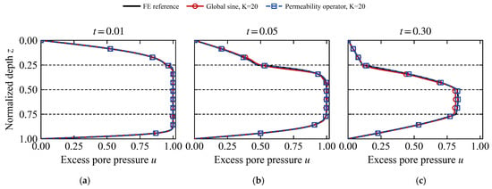
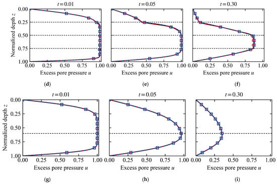
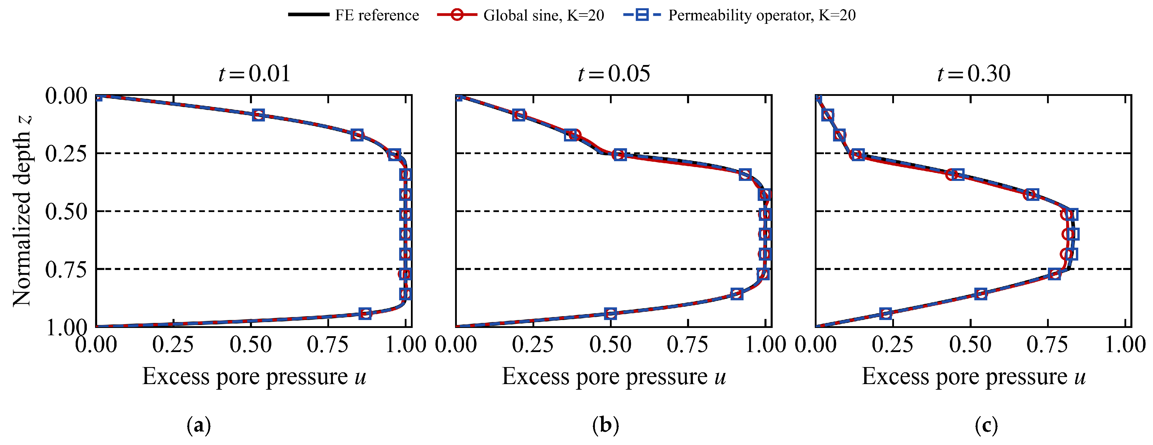
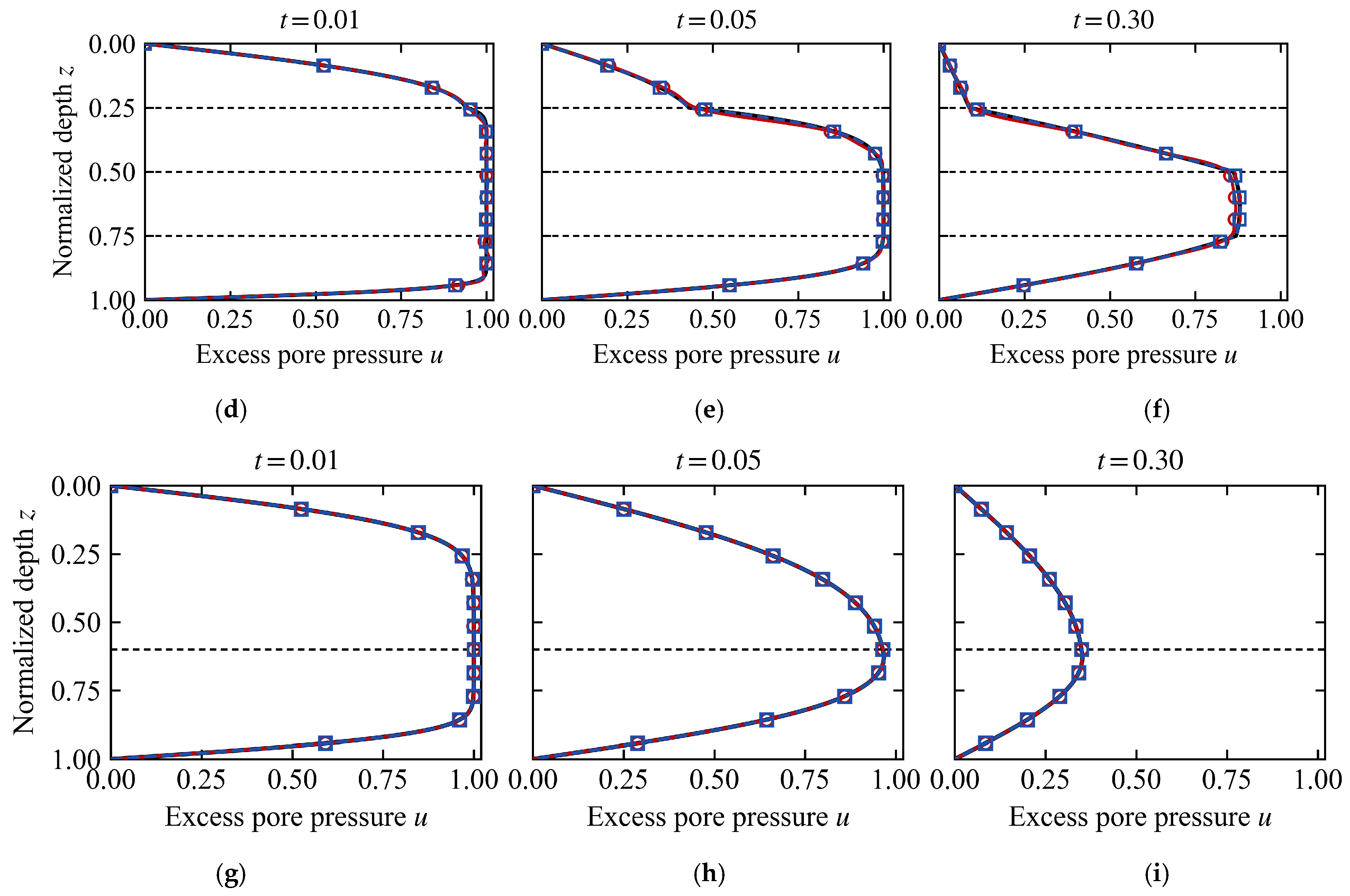
Selected pore pressure isochrones at K = 20 for the reference solution, the sine space, and the permeability-operator space are shown in Figure 3.

Figure 3. Pore pressure isochrones at K = 20. (a) S1, t = 0.01; (b) S1, t = 0.05; (c) S1, t = 0.30; (d) S2, t = 0.01; (e) S2, t = 0.05; (f) S2, t = 0.30; (g) S3, t = 0.01; (h) S3, t = 0.05; (i) S3, t = 0.30. Horizontal dashed lines mark the layer interfaces.

At K = 20 the permeability operator solution coincides with the finite element reference at all instants in the three cases. The deviation of the sine solution from the reference at the early instants, t = 0.01 and t = 0.05, is concentrated near the interfaces and the drainage end points, and by t = 0.30 it has essentially converged to the reference.

Let e_K(t) = u_K(t) − u_ref(t). For a set of time instants $𝒯$ with trapezoidal integration weights w_n, the relative space–time error is defined as

$$E_{\mathcal{T}}={\left[{\displaystyle \frac{{\sum }_{t_n\in \mathcal{T}}{w}_n{e}_K(t_n{)}^{\mathsf{T}}{M}_0{e}_K\left(t_n\right)}{{\sum }_{t_n\in \mathcal{T}}{w}_n{u}_{\mathrm{ref}}(t_n{)}^{\mathsf{T}}{M}_0{u}_{\mathrm{ref}}\left(t_n\right)}}\right]}^{1/2}$$

(36)

E_global uses all time levels in 0 ≤ t ≤ 1, including t = 0. Because the uniform initial value is incompatible with the drainage boundaries, the projection error at t = 0 and the transient that follows are concentrated in a layer of about 10⁻³ in time; E_[0.001,1] applies Equation (36) on t ≥ 0.001 and is reported alongside E_global. The interface band error also uses Equation (36), but the spatial integration is restricted to bands of half-width 0.02 on either side of each interface. The main comparison uses E_global and E_[0.001,1] under the unweighted projection. At K ≥ 40, E_global enters only through the mode numbers at the 10⁻² threshold, and the comparison relies on E_[0.001,1] and on the interface band error; between the two time grids compared in Section 4.1, the threshold mode numbers are unchanged and the interface band error changes by less than 4%.

4.3. Construction Verification and Finite Dimensional Performance

In S1, k_v/c_v = s, so the permeability operator modes are the exact continuous spectral modes described in Section 3.4. Numerically, at K = 80, ${‖B^{\left(P\right)}-\mathit{sI}‖}_F/{‖\mathit{sI}‖}_F=5.71\times {10}^{-16}$, which agrees with the analytical result of Equation (25). S1 therefore completes the verification of the operator-matched construction and its numerical implementation, whereas the finite dimensional performance comparison among the three spaces is carried out on the non-proportional case S2.

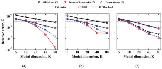
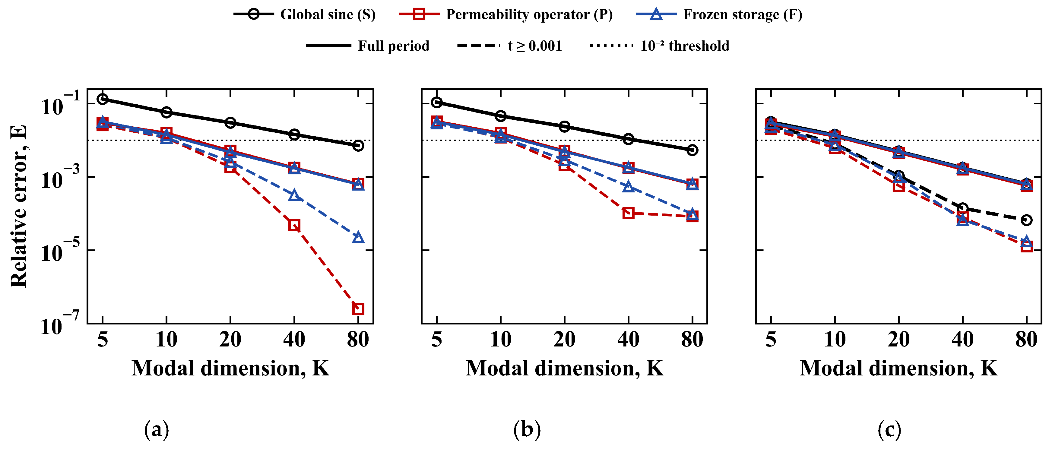
The convergence of E_global and E_[0.001,1] with the number of modes K is shown in Figure 4, and the first tested mode numbers that meet two error thresholds and the slopes of E_[0.001,1] fitted over K = 5–80 are summarized in Table 3.

Figure 4. Convergence of E_global (solid) and E_[0.001,1] (dashed) with K. (a) S1, (b) S2, and (c) S3.

Table 3. Mode numbers at two thresholds and fitted convergence slopes.

Case	Role	K at 10−2, Eglobal (S/P/F)	K at 10−2, E[0.001,1] (S/P/F)	K at 5 × 10−3, E[0.001,1] (S/P/F)	Slope of E[0.001,1] (S/P/F)
S1	sanity check	80/20/20	80/20/20	>80/20/20	−1.04/−4.12/−2.58
S2	performance	80/20/20	80/20/20	>80/20/20	−1.07/−2.38/−2.09
S3	boundary	20/20/20	10/10/10	20/20/20	−2.30/−2.75/−2.75

Note: S, P, and F denote the sine, permeability operator, and frozen storage spaces. Mode numbers are the first values in K ∈ 5, 10, 20, 40, 80 that meet the threshold. Slopes are fits over K = 5–80.

In S1 and S2 the curves of the two operator-adapted spaces lie below the sine curve throughout and first cross the 10⁻² reference line at K = 20, whereas the sine curve crosses it at K = 80. Excluding the initial layer widens this separation: E_[0.001,1] of the operator-adapted spaces decreases approximately as K^−2.1 to K^−4.1, while that of the sine space decreases approximately as K⁻¹ and remains close to its full-period value. In S3 the three curves are close for K ≥ 20. In S2 at K = 20, E_global for the sine, permeability operator, and frozen storage spaces is 2.39 × 10⁻², 5.16 × 10⁻³, and 4.85 × 10⁻³, and E_[0.001,1] is 2.36 × 10⁻², 2.13 × 10⁻³, and 2.92 × 10⁻³. The non-proportional condition also preserves the modal coupling of the permeability operator mass matrix, whose off-diagonal Frobenius ratio lies between 0.294 and 0.394 over K = 5–80. The K = 20 threshold result for S2 is therefore obtained in a coupled reduced-order system.

The two operator-adapted spaces are not uniformly ordered. The frozen storage space has the lower E_global, by 3% to 13%, for K = 10 and 20 in S1 and for K ≤ 20 in S2, whereas the permeability operator space has the lower E_[0.001,1] in 13 of the 15 case-dimension combinations. In both metrics the difference between them is small compared with their difference from the sine space: for K ≤ 20 the sine to permeability operator ratio of E_global is 3.7 to 5.8 in S1 and 3.0 to 4.6 in S2.

Although the permeability operator modes in S1 are the exact eigenfunctions of the continuous problem, their full-period error for K = 10 and 20 is not lower than that of the frozen storage space. The reason is that B^(P) = sI in S1, so the permeability operator space is an invariant subspace of the continuous operator, and its reduced-order solution equals the L² projection of the exact solution onto that space. The frozen storage space does not have this property, and its Galerkin solution is not the best approximation within its own subspace. The errors of the two constructions therefore cannot be judged solely by whether the basis is an exact eigenbasis. The final error depends jointly on how well the subspace approximates the solution and on the deviation of the Galerkin propagation, and these two contributions differ in magnitude between the two constructions.

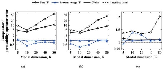
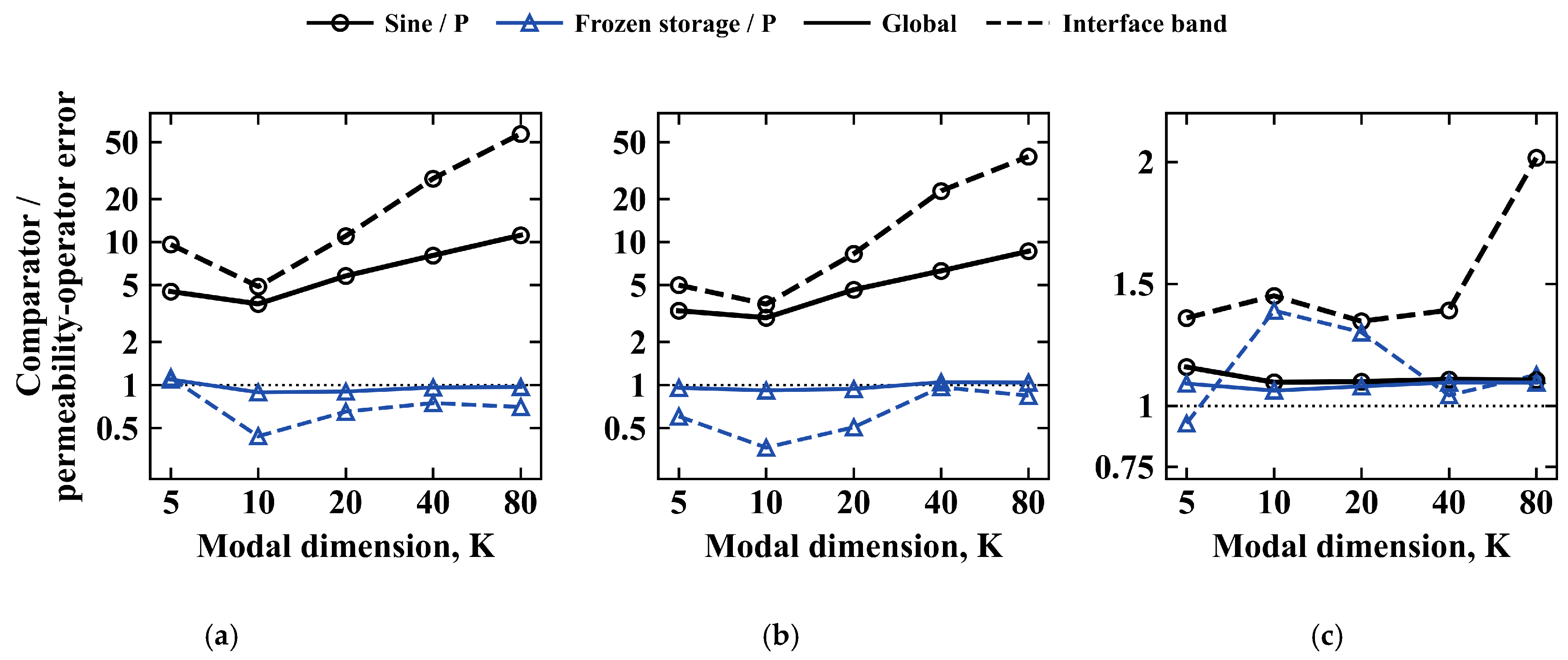
For the sine to permeability operator pair, as K increases from 20 to 80, the interface band error ratio increases from 11.0 to 57.2 in S1 and from 8.3 to 39.7 in S2. The residual error of the sine space near the interfaces therefore decreases much more slowly with K than that of the permeability operator space.

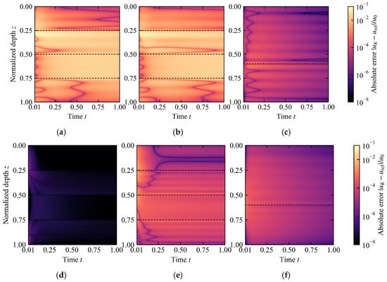
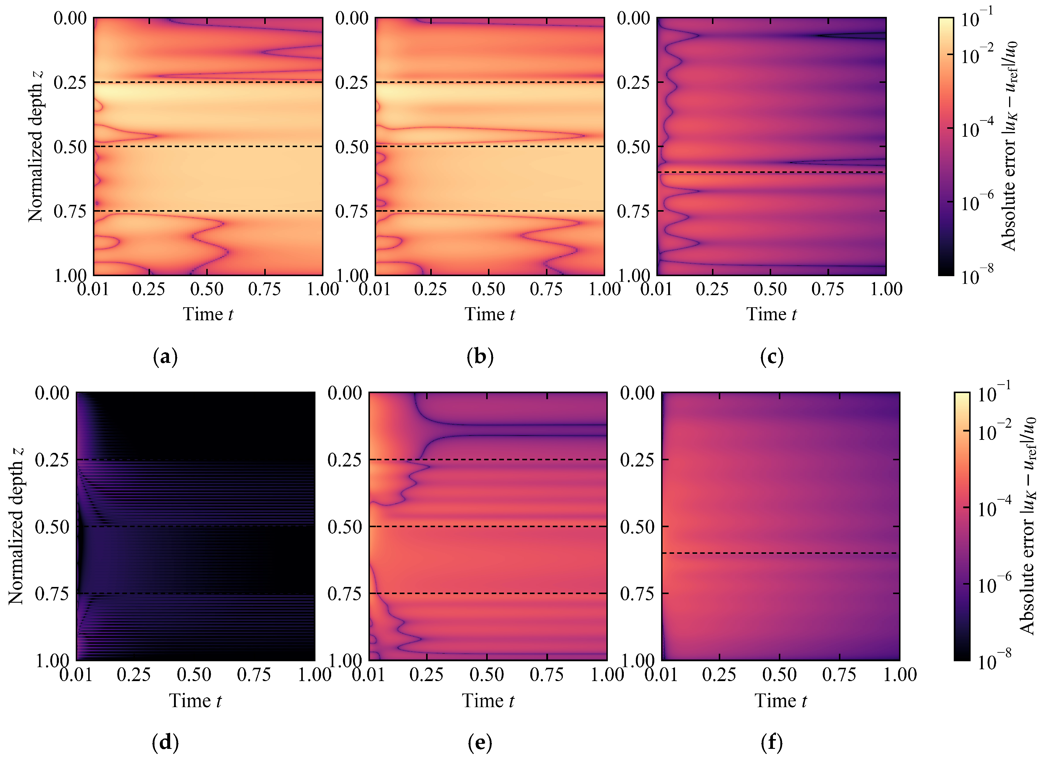
The space–time absolute error fields of the global sine space and the permeability operator space at K = 20 for the three cases are shown in Figure 5, in which all subplots use the same mesh, output instants, and color normalization.

Figure 5. Space–time absolute errors at K = 20. (a) S1: global sine space; (b) S2: global sine space; (c) S3: global sine space; (d) S1: permeability operator space; (e) S2: permeability operator space; (f) S3: permeability operator space. Dashed lines mark the layer interfaces.

The residual errors of the two spaces have distinctly different space–time distributions in the high-contrast configurations. In S1 and S2, the error of the sine space persists along depth over the entire time interval and forms bands at the three interfaces that extend through the whole period (Figure 5a,b), whereas the error of the permeability operator space is concentrated in the early stage t ≲ 0.05 and then decays rapidly, without forming persistent bands at the interfaces (Figure 5d,e). S3 differs (Figure 5c,f): the error fields of the two spaces are close in both magnitude and distribution, and no marked contrast appears at the interfaces. The former is consistent with the growth of the interface band error ratio with K. The residual error of the sine space remains anchored at the interfaces, while that of the operator-adapted space is mainly an early transient.

4.4. Material Contrast and Projection Sensitivity

In S3 the material contrast is reduced from 10 to 2, and the three spaces require the same number of modes at both error thresholds (Table 3). Because S3 also differs from S1 and S2 in the number of layers, the interface position, and c_v, the effect of contrast is isolated with the fixed geometry sweep (Table 4): the operator-adapted spaces first reach E_global = 10⁻² at K = 20 for every κ, whereas the sine space requires 20 modes at κ ≤ 2, 40 at κ = 5, 80 at κ = 10 and 20, and more than 80 at κ = 50. The reduced-order gain of the operator-adapted spaces therefore increases with material contrast. At a contrast of 2 the three spaces are equivalent, and the sine space is then simpler because its matrices can be assembled analytically. Two-layer foundations of this kind arise in practice when a treated surface layer overlies natural ground [34]. Under the main projection, the frozen storage error is slightly higher than the permeability operator error for K ≤ 20, with $E_{\mathrm{global}}^{\left(P\right)}/E_{\mathrm{global}}^{\left(F\right)}$ between 0.92 and 0.94.

Table 4. First tested mode numbers at E_global = 10⁻² and error ratio at K = 20 in the contrast sweep.

κ	K at 10−2 (S/P/F)	${\mathit{E}}_{\mathbf{global}}^{\left(\mathit{S}\right)}/{\mathit{E}}_{\mathbf{global}}^{\left(\mathit{P}\right)}$, K = 20
1	20/20/20	1.00
2	20/20/20	1.13
5	40/20/20	2.64
10	80/20/20	4.63
20	80/20/20	7.27
50	>80/20/20	7.38

Over K = 5–80, E_[0.001,1] of both operator-adapted spaces decreases faster than that of the sine space in all three cases (Table 3). In S1 the permeability operator error at K = 80 reaches the resolution of the modal discretization, about 2 × 10⁻⁷, which steepens its fitted slope. Under the S-weighted projection, the global sine to permeability operator error ratio for K ≤ 20 spans nearly the same range as under the main projection. S is constant in S1, so the two projections are identical there. In S2 the projection rule changes several ratios: E^(P)/E^(F) at K = 5 changes from 1.05 to 0.93, and the ordering of the two operator-adapted candidates is reversed.

The error ratios under different metrics are shown in Figure 6.

Figure 6. Error ratios relative to the permeability-operator space. (a) S1; (b) S2; (c) S3.

In S1 and S2, for K ≤ 20 the sine to permeability operator interface band ratio exceeds the global ratio, and both ratios decrease from K = 5 to K = 10 and increase from K = 10 to K = 20; the interface band ratio continues to increase up to K = 80. For K ≤ 20 the frozen storage to permeability operator global ratio stays between about 0.9 and 1.1. The reversal of ordering under a change of projection observed for S2 at K = 5 indicates that the reduced-order gain relative to the sine space and the choice between the two operator-adapted candidates are two questions that should be evaluated separately.

5. Forward Verification and Inverse Solver Selection

5.1. Forward Verification with Known Parameters in the Non-Proportional Case

Before proceeding to parameter inversion, the non-proportional two-layer case k_v = [2, 1], c_v = [0.6,0.2] is used to examine whether the neural time coefficient parameterization can solve the reduced-order dynamical system when the material parameters are known. The test uses K = 10 and three fixed random seeds and keeps the network, the hard initial condition, the modal scaling, the sampling, and the optimization budget unchanged, adding only a fixed residual row preconditioner.

Relative to the K = 10 matrix exponential reduced-order solution, the median modal error over the three random seeds was 4.41 × 10⁻⁴, and the reconstructed field error was 4.41 × 10⁻⁴. The ratio of the maximum modal error to the median was 1.135. These values satisfy the accuracy limit of 2 × 10⁻³ and the stability limit requiring the ratio of the maximum to the median modal error not to exceed 3.

Changing the residual row scaling alone reduced the median modal error from 3.98 × 10⁻³ to 4.41 × 10⁻⁴, a factor of 9.03. With Adam alone, the final errors of the three runs were 9.32 × 10⁻³, 9.82 × 10⁻³, and 6.76 × 10⁻³. Reaching the forward accuracy limit required L-BFGS with fixed collocation points and a strong Wolfe line search. The same forward check was repeated for the four-layer configurations S1 and S2 with the network and training procedure unchanged, giving median modal errors of 2.92 × 10⁻⁴ and 5.18 × 10⁻⁴ and maximum-to-median ratios of 2.11 and 1.32, within both limits.

5.2. Inverse Configurations and Local Numerical Sensitivity

Inverse configurations A, B, and C use the same three material settings as in Section 4.2: A corresponds to S3, B to S1, and C to S2. The suffixes dense and sparse correspond to the two observation layouts in Figure 1. The sensors are located at z = 0.10, 0.55, and 0.65 in A; at z = 0.10, 0.20, 0.30, 0.45, 0.55, 0.70, and 0.80 in B-dense and C-dense; and at z = 0.10, 0.30, 0.45, 0.55, and 0.80 in C-sparse. The dense layouts observe at t = 0.01, 0.02, …, 1.00 and the sparse layouts at 25 equally spaced instants from t = 0.01 to 1.00. The two initial values are c_v = 0.1414 in every layer, the logarithmic midpoint of the bounds, and c_v = [0.3492, 0.0573] in A and [0.3492, 0.0573, 0.3492, 0.0573] in B and C. A local numerical Jacobian is computed at each given parameter vector to check the local sensitivity of the inverse configurations. Each column is obtained by central finite differences with respect to log c_v,𝓁, and every perturbed observation is recomputed with an independent 1601-node full-order finite element model with backward Euler at Δt = 1/6400. The logarithmic step size is reduced progressively from 10⁻² to 1.25 × 10⁻³, and the relative change between the Jacobians at the two finest levels ranges from 5.35 × 10⁻⁷ to 8.33 × 10⁻⁷. The reported singular value decomposition uses the finest step size.

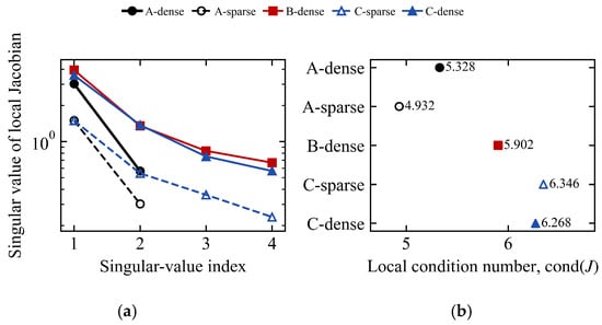
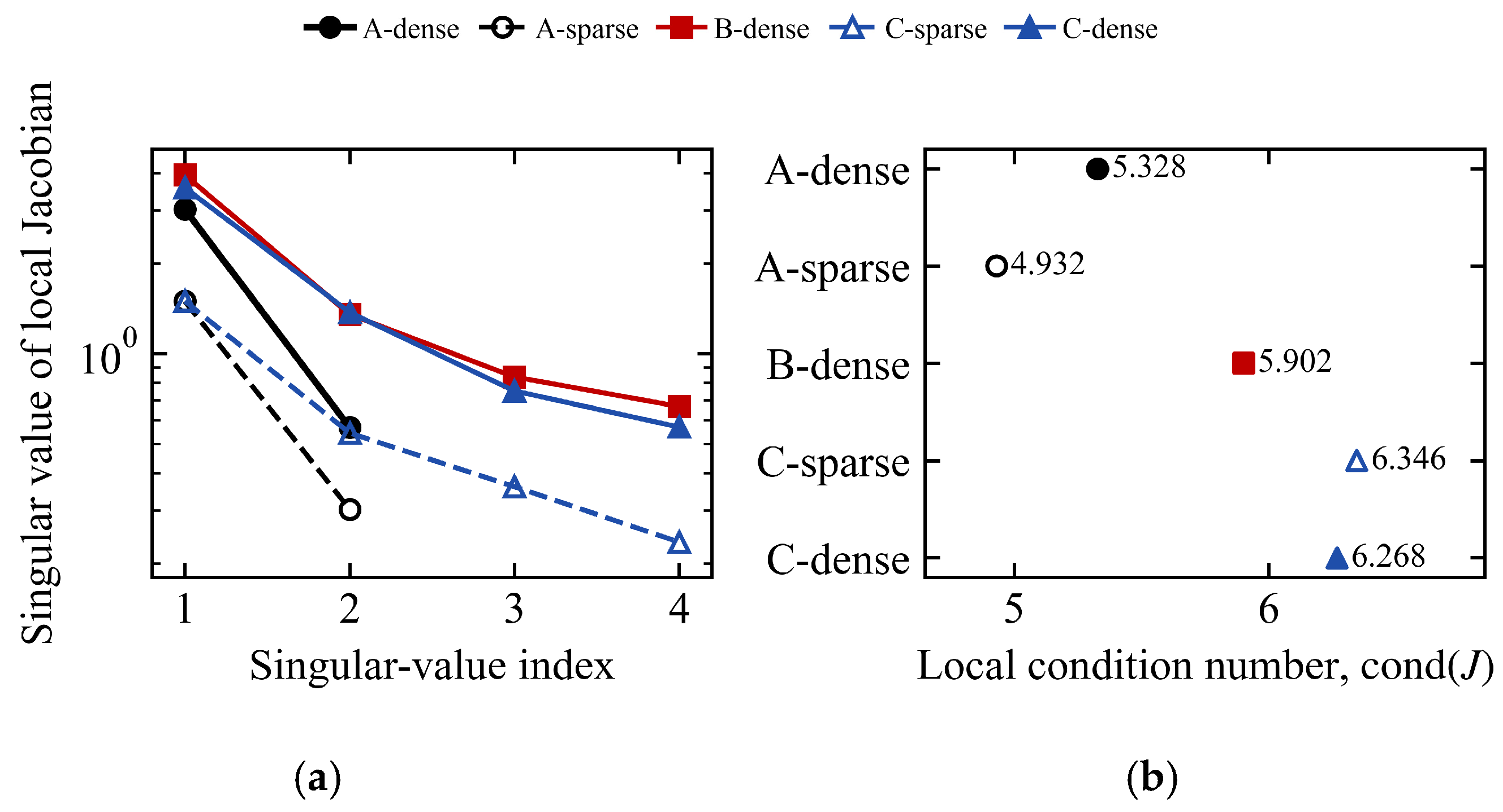
The singular values are scaled by the unit normalized observation standard deviation, which allows for the local sensitivity directions to be compared. A-sparse contains 75 observations for two unknowns, and C-sparse contains 125 observations for four unknowns, so both are overdetermined configurations. The singular value spectra and the condition numbers of the local Jacobians for the five inverse configurations are shown in Figure 7.

Figure 7. Local sensitivity of the inverse configurations. (a) Jacobian singular values; (b) local condition numbers.

When the observation times are reduced from dense to sparse, all singular values of A and C decrease together, while the condition numbers do not increase substantially. Sparsification therefore lowers the overall sensitivity rather than selectively weakening a particular direction. The smallest singular value of C increases from 0.236 in the sparse configuration to 0.570 in the dense configuration. The weakest right singular direction of its sparse configuration is [0.563, −0.810, 0.167, −0.011], whose amplitude is concentrated in a combination of the first and second layers with opposite signs. This configuration is therefore least sensitive to perturbations of c_v in the first two layers that have opposite signs.

5.3. Classical Reduced-Order Inversion and Verification of the Observation Data

The classical inversion propagates the K = 10 permeability operator reduced-order system through Equation (31) and minimizes the observation residual in log c_v by bounded least squares. The optimizer is the trust region reflective algorithm with a three-point finite difference Jacobian, function, step, and gradient tolerances of 10⁻¹², and at most 500 function evaluations. The parameter bounds, the two initial values, the sensors, the observation times, and the full-order finite element data are the same as in the neural inversion. Every identified parameter vector is recomputed with an independent full-order finite element model.

For run r, the mean and maximum layer parameter errors are defined as

$$E_c^{\left(r\right)}={\displaystyle \frac{1}{L}}{\sum }_{\mathcal{l}=1}^L\left|{\displaystyle \frac{c_{v,\mathcal{l}}^{\left(r\right)}-c_{v,\mathcal{l}}^{\mathrm{true}}}{c_{v,\mathcal{l}}^{\mathrm{true}}}}\right|,E_{c,\max }^{\left(r\right)}={\max }_{\mathcal{l}}\left|{\displaystyle \frac{c_{v,\mathcal{l}}^{\left(r\right)}-c_{v,\mathcal{l}}^{\mathrm{true}}}{c_{v,\mathcal{l}}^{\mathrm{true}}}}\right|$$

(37)

and the independently recomputed full-field error is

$$E_{\mathrm{FE}}^{\left(r\right)}={\left[{\displaystyle \frac{{\sum }_n{‖{\mathbf{u}}_{\mathrm{FE}}\left(t_n;c_v^{\left(r\right)}\right)-{\mathbf{u}}_{\mathrm{FE}}\left(t_n;{\mathbf{c}}_v^{\mathrm{true}}\right)‖}_2^2}{{\sum }_n{‖{\mathbf{u}}_{\mathrm{FE}}\left(t_n;{\mathbf{c}}_v^{\mathrm{true}}\right)‖}_2^2}}\right]}^{1/2}$$

(38)

The sensor observation error, obtained after applying the prescribed sensor interpolation operator, uses the same relative Frobenius form. The classical results report the median of the two initial-value runs, which coincide to at least four significant digits, and the neural results in Section 5.4 are the median of six runs.

The observation data used for inversion were first reproduced independently and then verified on the 1601-, 3201-, and 6401-node meshes. The relative change in the observations from 1601 to 3201 nodes was 3.81 × 10⁻⁷ to 6.77 × 10⁻⁷, and that from 3201 to 6401 nodes was 9.62 × 10⁻⁸ to 1.69 × 10⁻⁷, which corresponds to observation convergence orders of 1.988 to 2.003. Direct mesh refinement shows that the spatial discretization component is two to three orders of magnitude below the estimate of 4 × 10⁻⁴ obtained from the mesh size alone through h². On the 6401-node mesh, the difference between the backward Euler and the Rannacher–Crank–Nicolson observations was 2.41 × 10⁻⁴ to 7.45 × 10⁻⁴, which shows that the first-order time integrator is the dominant component of the discretization error in the observation source data.

The classical inversion errors are placed alongside the empirical source data error bounds in Table 5. Each bound is the sum of three relative differences: the change from 1601 to 6401 nodes with backward Euler, the change from backward Euler to Rannacher–Crank–Nicolson on the 6401-node mesh, and the change of the latter when Δt is halved.

Table 5. Classical inversion errors and observation source numerical verification bounds.

Configuration	Layer Mean Error (%)	Maximum Layer Error (%)	FE Observation Error (%)	FE Full-Field Error (%)	Source Observation Bound (%)	Source Field Bound (%)
A-dense	0.116	0.206	0.0502	0.0722	0.0503	0.0469
A-sparse	0.275	0.369	0.0746	0.0927	0.0747	0.0619
B-dense	0.196	0.427	0.0246	0.0291	0.0247	0.0252
C-sparse	2.115	3.915	0.0354	0.3030	0.0355	0.0329
C-dense	0.445	1.392	0.0241	0.1850	0.0242	0.0244

Both classical initial values converged to similar estimates. The largest parameter error occurred in C-sparse, whose layer errors were [3.915%, 2.953%, 0.690%, 0.901%], while the corresponding values for C-dense were [0.068%, 0.253%, 0.066%, 1.392%].

To measure the effect of the source data directly, the five inversions were repeated with observations regenerated by the reference model of Section 4.1, and each identified parameter vector was recomputed with the same model. The regenerated observations differ from the original ones by 0.024% to 0.074%, in agreement with the source observation bounds in Table 5. The layer mean parameter error changes by at most 0.22 percentage points: from 0.116% to 0.054% in A-dense, 0.275% to 0.054% in A-sparse, 0.196% to 0.116% in B-dense, 2.115% to 1.960% in C-sparse, and 0.445% to 0.476% in C-dense.

The classical inversion was repeated with the three spaces at K ∈ 5, 10, 20, 40, 80, using observations so that the remaining parameter error reflects the truncation of the space (Table 6). With the permeability operator space, the layer mean error at K = 10 is 0.05% in A and 0.12% to 1.96% in B and C. It decreases to at most 0.32% at K = 20 and at most 0.03% at K = 40. At K = 10 the estimates therefore partly compensate for the truncation of the space, mainly in the four-layer configurations. The frozen storage space gives errors of the same order: lower than the permeability operator space in C at K = 20, and higher in A and B. At the dimensions at which the forward error first reaches 10⁻² (Table 3), the sine space gives layer mean errors of 2.06% to 2.27% in B and C at K = 80, compared with at most 0.32% for the operator-adapted spaces at K = 20. In A, where all three spaces reach that threshold at K = 20, the errors are 0.11% to 0.12% for the sine space and 0.03% to 0.08% for the operator-adapted spaces. The online time per inversion was measured single-threaded, with an implementation that solves Equation (30) once for each candidate and evaluates Equation (31) at all observation instants. At these dimensions it is 0.063–0.089 s for the sine space and 0.020–0.032 s for the operator-adapted spaces in B and C; in A the sine space is the fastest because its matrices are assembled analytically. With the original observations, the permeability operator errors level off at 0.09% to 0.28% from K = 40, which is the level set by the time discretization of the source data.

Table 6. Layer mean parameter error (%) of the classical inversion with the three spaces and the rebuilt eigenbasis.

Configuration	P, K = 10/20/40	F, K = 10/20/40	S, K = 20/80	Rebuilt, K = 10/20
A-dense	0.054/0.028/0.007	0.143/0.082/0.007	0.122/0.036	0.011/<0.001
A-sparse	0.054/0.028/0.007	0.129/0.069/0.007	0.105/0.030	0.038/<0.001
B-dense	0.116/<0.001/<0.001	0.925/0.174/0.030	10.3/2.10	0.208/<0.001
C-sparse	1.96/0.255/0.025	1.12/0.119/0.091	11.8/2.06	2.13/<0.001
C-dense	0.476/0.322/0.020	0.931/0.131/0.094	11.6/2.27	0.087/<0.001

Observation noise and errors in the assumed layer profile were examined with the permeability operator space at K = 20 and the regenerated observations. Independent Gaussian noise with standard deviation ηU_scale, η ∈ 0.5%, 1%, 2%, 5%, was added to the observations, and each configuration was inverted for 100 noise realizations from the first initial value. The standard deviation of the layer errors increases in proportion to η and is largest in the sparse layouts, and the bias remains below 0.9% for η ≤ 2%. Four of the C-sparse inversions at η = 5% reached a parameter bound. With noise-free observations, the assumed profile was then perturbed by changing the permeability of the more permeable layers by ±5% to ±20%, or by shifting all interfaces by ±0.005 to ±0.02. In A, the layer mean error remains below 1.6% for all perturbations. In B and C, it is 2.1–2.5% for a 5% permeability error and 5.5–9.2% for an interface shift of 0.005 and reaches 46% for a shift of 0.02.

As a reference for fixing the space, the classical layered eigenbasis was rebuilt at every objective evaluation from $-{\left(k_v{q}^{\prime }\right)}^{\prime }=\mathit{\omega S}\left(c_v\right)q$ with the candidate storage weight on the same 3201-node mesh, and the initial condition was projected in the S-weighted inner product, under which these modes decouple. At K = 20 its layer mean error is below 0.001% in all five configurations, whereas that of the fixed operator-adapted spaces is at most 0.32% (Table 6). With the same implementation, rebuilding raises the online time per inversion from 0.016–0.027 s for the permeability operator space to 0.85–1.75 s. Fixing the space thus trades a truncation error of at most 0.32% at K = 20 for a 50- to 70-fold reduction in online cost. This error is smaller than the parameter scatter obtained with 0.5% observation noise (Table 7).

Table 7. Parameter errors under observation noise: largest absolute bias/largest standard deviation over the layers (%).

Configuration	η = 0.5%	η = 1%	η = 2%	η = 5%
A-dense	0.06/0.64	0.10/1.28	0.20/2.56	0.70/6.44
A-sparse	0.04/1.34	0.10/2.71	0.41/5.59	3.49/17.2
B-dense	0.05/0.54	0.11/1.08	0.25/2.15	0.84/5.38
C-sparse	0.39/1.84	0.44/3.70	0.87/7.57	4.65/22.6
C-dense	0.72/0.81	0.74/1.63	0.77/3.28	0.78/8.45

5.4. Inversion Results and Solver Comparison

The solver comparison comprises 30 neural runs, obtained from three random seeds and two initial values for each configuration, and 10 classical runs using the same two initial values. The neural results below are the median of six runs for each configuration, with the range over the six runs given in brackets in Table 8, and the classical results are the median of two runs. A run is counted as failed if the optimizer terminates abnormally, the loss becomes non-finite, or an identified parameter lies on a bound; none of the 30 neural and 10 classical runs failed. The total wall clock time includes the offline basis construction, the neural training or the classical inversion, and the full-order finite element verification. The offline construction takes 0.10–0.44 s and the verification 0.85–4.4 s for both solvers. The online stage takes 317–596 s for neural training, with an interquartile range of 14–79 s over the six runs, and 0.43–3.93 s for the classical inversion, which requires 9.5–12 objective evaluations on average. These classical runs used K = 10 and the default library threading and computed the propagation by a dense matrix exponential at each observation instant, whereas the times in Section 5.3 refer to K = 20 (K = 80 for the sine space in B and C) and to the single-threaded implementation described there, with the same optimizer settings. With that implementation, the classical inversion at K = 10 takes 0.010–0.019 s with a similar number of objective evaluations. All these times cover the online inversion only, without the offline construction and the full-order verification. Because the neural and classical runs used the GPU and the CPU, respectively, the time ratios in Table 8 depend on the hardware and the implementation.

Table 8. Inverse solver comparison for the five configurations.

Configuration	Observations/Unknowns	Cond (J)	Parameter Error Neural/Classical (%)	FE Field Error Neural/Classical (%)	Total Time Neural/Classical (s)	Time Ratio
A-dense	300/2	5.328	2.581 [1.52, 3.51]/0.116	0.662 [0.39, 0.89]/0.072	601.5/2.61	230×
A-sparse	75/2	4.932	2.358 [0.77, 2.95]/0.275	0.649 [0.21, 1.41]/0.093	339.7/1.49	227×
B-dense	700/4	5.902	1.850 [1.51, 2.25]/0.196	0.466 [0.29, 0.51]/0.029	341.8/3.90	88×
C-sparse	125/4	6.346	4.840 [3.85, 5.60]/2.115	0.723 [0.59, 0.75]/0.303	346.1/2.60	133×
C-dense	700/4	6.268	0.747 [0.45, 1.26]/0.445	0.294 [0.25, 0.40]/0.185	319.2/5.72	56×

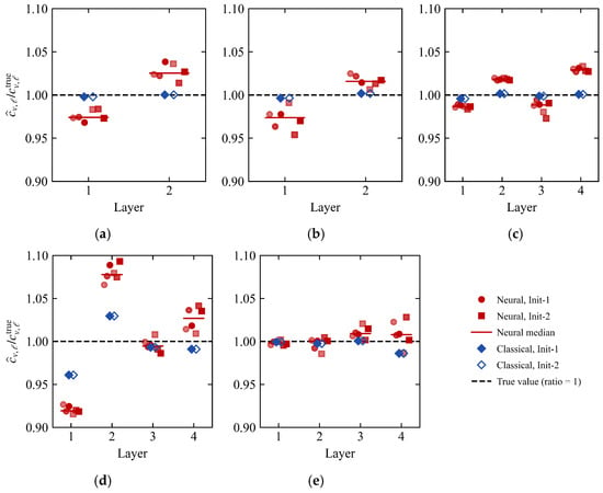
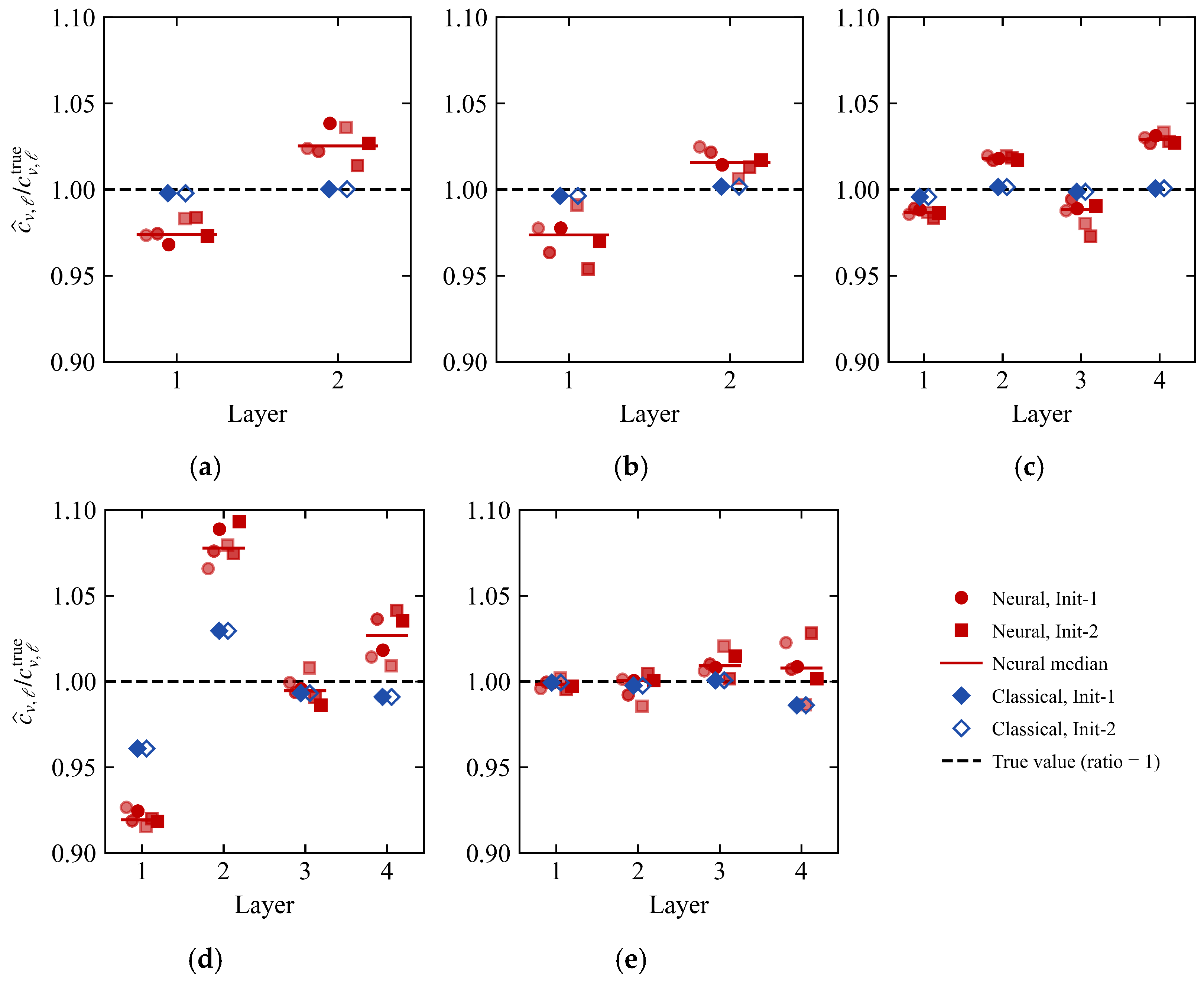
The run-by-run coefficient recovery is shown in Figure 8, and the solver comparison is summarized in Table 8.

Figure 8. Recovery of layer-wise consolidation coefficients. (a) A-dense; (b) A-sparse; (c) B-dense; (d) C-sparse; (e) C-dense.

The classical estimates cluster near the true values in all five configurations, and the two initial values almost coincide, whereas the neural estimates exhibit a systematic rather than random offset. This is clearest in C-sparse (Figure 8d), where the first-layer estimate is uniformly low and the second-layer estimate uniformly high. The two deviations have opposite signs and the largest amplitudes, and their sign structure agrees with that of the weakest right singular direction of this configuration given in Figure 7. Projecting the logarithmic parameter error vectors onto the right singular vectors shows that the weakest direction carries a median of 84% to 99% of the squared error of the neural runs in A-dense, A-sparse, B-dense, and C-sparse, but 2% in C-dense. The residual error of the neural solution therefore falls mainly along the least sensitive direction of the local Jacobian in four of the five configurations.

The fixed training settings were varied one at a time for C-sparse, with six runs per variant: the data weight was set to 10 or 1000 instead of 100, the numbers of collocation points in both stages were halved or doubled, and the Adam and L-BFGS iteration budgets were halved or doubled. The median layer mean parameter error of the variants lies between 3.98% and 5.32%, compared with 4.84% for the baseline setting and 2.115% for the classical inversion. The median field error lies between 0.46% and 0.82%, compared with 0.303% for the classical inversion.

In all five configurations, the layer mean parameter error, the independently recomputed finite element full-field error, and the recorded total wall clock time of the classical reduced-order inversion are all lower. The recorded total wall clock time of the neural approach is 56 to 230 times that of the classical method.

6. Conclusions

Two operator-adapted modal spaces that can be reused offline are constructed in this study for the forward modeling that underlies the inversion of layered coefficients of consolidation. The permeability operator basis is generated by an unweighted mass eigenvalue problem, and the frozen storage basis uses a storage weight proportional to k_v. The two are compared with the Walker-type global sine space under a unified projection, propagation, and full-order finite element reference. Within the same permeability operator space, direct matrix propagation and neural time coefficient parameterization are further compared as two online solvers. The main conclusions are as follows:

(1) Both bases depend only on the layer positions and the relative k_v profile and remain fixed and reusable throughout the inversion. A candidate c_v enters the reduced-order system only through the modal mass matrix assembled from the layer Gram matrices. This matrix is affine in 1/c_v, so each candidate parameter set requires only O(LK²) operations to assemble, without returning to the full-order mesh. A common scaling of k_v leaves the trial space unchanged. This construction satisfies both requirements that the forward model of an inversion places on the space representation, namely fixed reuse and compatibility with the interface flux. The flux condition holds exactly for the continuous modes and in the variational sense for the P1 modes, whose recovered one-sided flux jump decreases at first order under mesh refinement. Compared with the classical eigenbasis rebuilt for each candidate, fixing the space leaves a layer mean parameter error of at most 0.32% at K = 20 and reduces the online cost by a factor of 50 to 70.

(2) In the high-contrast four-layer configuration, the operator-adapted spaces first reach E_global = 10⁻² at K = 20 among the dimensions tested, whereas the sine space first meets this threshold at K = 80. After the initial layer, their errors decrease approximately as K^−2.1 to K^−4.1, against about K⁻¹ for the sine space, and the advantage over the sine space, measured by the interface band error, grows with K beyond K = 10. The two operator-adapted spaces are of comparable accuracy, and neither is uniformly lower. The reduced-order gain does not require the temporal decoupling of the proportional case. S1 satisfies B^(P) = sI and its reduced-order equations decouple completely, whereas S2 retains modal coupling, with an off-diagonal Frobenius ratio of 0.294 to 0.394 yet achieves the same threshold reduction. The operator-matching identity characterizes temporal decoupling in the weighted coordinates, while the reduced-order gain arises from how well the subspace approximates the solution; these are two independent properties. The gain appears in the high-contrast configurations and, at fixed geometry, increases with material contrast. At matched forward accuracy, the operator-adapted spaces also give parameter errors about an order of magnitude below those of the sine space in the four-layer configurations. In the two-layer low-contrast configuration S3, the three spaces require the same number of modes, and the sine space is then simpler because its matrices can be assembled analytically.

(3) In the five observation configurations, matrix propagation combined with bounded least squares gives lower parameter errors and lower full-order field errors than neural time coefficient parameterization, at 1/230 to 1/56 of its computational time on the hardware used here. The neural approach passed the accuracy threshold of the forward problem with known parameters, which shows that it is workable, but it offers no benefit under the network architecture and training scheme used here. For linear reduced-order inversions with two to four parameters to be identified, matrix propagation combined with bounded least squares should be preferred. The space representation and the online algorithm can be selected separately, the former according to the layered operator and the latter according to the structure of the reduced-order dynamical system. Both solvers were compared at K = 10, at which the classical estimates in the four-layer configurations still contain a truncation component; at K = 20 the classical layer mean error is at most 0.32%.

The present work is restricted to linear one-dimensional consolidation. The interfaces and the relative k_v profile are taken as known, and c_v of each layer is the quantity to be identified. The identification is sensitive to errors in the interface positions: in the four-layer configurations, a dimensionless interface shift of 0.005 produces layer mean parameter errors of 5.5–9.2%, and a shift of 0.02 produces errors of up to 46%. For the 5 m column of Section 2.2, these shifts correspond to 2.5 cm and 10 cm, so field applications require the interface positions to be determined accurately. Since c_v = k_v/(m_vγ_w), this setting corresponds to the identification of relative compressibility under a known relative permeability profile. Because the absolute permeability scale is not identified, c_v alone does not determine the absolute compressibility or the settlement magnitude. The observations are generated by numerical models and contain no field noise, so the comparison is confined to the reduced-order representation and the online algorithms themselves. Instantaneous loading and perfect drainage at both boundaries are assumed, and k_v and m_v are independent of stress; in field data, partial drainage, uncertain or staged loading, and stress-dependent properties would be absorbed into the identified c_v and bias it. S1 and S2 share the same layer geometry and relative k_v profile, so the modal thresholds reported for them are reproducible under a fixed configuration. S3 differs from them in the number of layers, the interface position, and the material contrast at the same time, so the effect of contrast was examined separately by varying the permeability ratio at fixed geometry; other layer arrangements and thickness ratios were not examined. Uncertainty in the k_v profile, noisy field data, and nonlinear and multidimensional settings are directions for future work.

References

- Terzaghi, K. Theoretical Soil Mechanics; John Wiley & Sons: New York, NY, USA, 1943. [Google Scholar] [CrossRef] [Scilit]
- Olek, B.S. State-of-the-Art Review on Determining One-Dimensional Consolidation Parameters Based on Compression and Distribution of Pore Water Pressure: Coefficient of Consolidation (cv), End of Primary (EOP) Consolidation. Arch. Comput. Methods Eng. 2025, 32, 605–644. [Google Scholar] [CrossRef] [Scilit]
- Gong, W.; Zuo, L.; Li, L.; Wang, H. Prediction of stratified ground consolidation via a physics-informed neural network utilizing short-term excess pore water pressure monitoring data. Comput.-Aided Civ. Infrastruct. Eng. 2025, 40, 147–165. [Google Scholar] [CrossRef] [Scilit]
- Hong, S.; Kim, S.-R. Physics-informed neural networks for back-analysis and consolidation settlement prediction using field measurements. Acta Geotech. 2026, 21, 2309–2342. [Google Scholar] [CrossRef] [Scilit]
- Schiffman, R.L.; Stein, J.R. One-Dimensional Consolidation of Layered Systems. J. Soil Mech. Found. Div. 1970, 96, 1499–1504. [Google Scholar] [CrossRef] [Scilit]
- Lee, P.K.K.; Xie, K.H.; Cheung, Y.K. A study on one-dimensional consolidation of layered systems. Int. J. Numer. Anal. Methods Geomech. 1992, 16, 815–831. [Google Scholar] [CrossRef] [Scilit]
- Xie, K.-H.; Xie, X.-Y.; Gao, X. Theory of one dimensional consolidation of two-layered soil with partially drained boundaries. Comput. Geotech. 1999, 24, 265–278. [Google Scholar] [CrossRef] [Scilit]
- Zong, M.; Wu, W.; El Naggar, M.H.; Mei, G.; Zhang, Y. Analysis of One-Dimensional Consolidation for Double-Layered Soil with Non-Darcian Flow Based on Continuous Drainage Boundary. Int. J. Geomech. 2023, 23, 04022306. [Google Scholar] [CrossRef] [Scilit]
- Zong, M.; Zhang, J.; Wu, W.; Zhang, Y.; Mei, G. Semi-analytical solution for one-dimensional consolidation of multi-layered soil considering non-Darcian flow and multi-stage loading under continuous drainage boundary. Comput. Geotech. 2024, 169, 106192. [Google Scholar] [CrossRef] [Scilit]
- Walker, R.; Indraratna, B.; Sivakugan, N. Vertical and Radial Consolidation Analysis of Multilayered Soil Using the Spectral Method. J. Geotech. Geoenviron. Eng. 2009, 135, 657–663. [Google Scholar] [CrossRef] [Scilit]
- Walker, R.T.R.; Indraratna, B. Application of spectral Galerkin method for multilayer consolidation of soft soils stabilised by vertical drains or stone columns. Comput. Geotech. 2015, 69, 529–539. [Google Scholar] [CrossRef] [Scilit]
- Xu, B.-H.; Indraratna, B.; Rujikiatkamjorn, C.; Yin, J.-H.; Kelly, R.; Jiang, Y.-B. Consolidation analysis of inhomogeneous soil subjected to varied loading under impeded drainage based on the spectral method. Can. Geotech. J. 2025, 62, 1–21. [Google Scholar] [CrossRef] [Scilit]
- Quarteroni, A.; Manzoni, A.; Negri, F. Reduced Basis Methods for Partial Differential Equations: An Introduction; Springer: Cham, Switzerland, 2016. [Google Scholar] [CrossRef] [Scilit]
- Efendiev, Y.; Galvis, J.; Hou, T.Y. Generalized multiscale finite element methods (GMsFEM). J. Comput. Phys. 2013, 251, 116–135. [Google Scholar] [CrossRef] [Scilit]
- Carr, E.J.; Turner, I.W. A semi-analytical solution for multilayer diffusion in a composite medium consisting of a large number of layers. Appl. Math. Model. 2016, 40, 7034–7050. [Google Scholar] [CrossRef] [Scilit]
- Raissi, M.; Perdikaris, P.; Karniadakis, G.E. Physics-informed neural networks: A deep learning framework for solving forward and inverse problems involving nonlinear partial differential equations. J. Comput. Phys. 2019, 378, 686–707. [Google Scholar] [CrossRef] [Scilit]
- Karniadakis, G.E.; Kevrekidis, I.G.; Lu, L.; Perdikaris, P.; Wang, S.; Yang, L. Physics-informed machine learning. Nat. Rev. Phys. 2021, 3, 422–440. [Google Scholar] [CrossRef] [Scilit]
- Wang, S.; Teng, Y.; Perdikaris, P. Understanding and mitigating gradient flow pathologies in physics-informed neural networks. SIAM J. Sci. Comput. 2021, 43, A3055–A3081. [Google Scholar] [CrossRef] [Scilit]
- Rezaei, S.; Harandi, A.; Moeineddin, A.; Xu, B.-X.; Reese, S. A mixed formulation for physics-informed neural networks as a potential solver for engineering problems in heterogeneous domains: Comparison with finite element method. Comput. Methods Appl. Mech. Eng. 2022, 401, 115616. [Google Scholar] [CrossRef] [Scilit]
- Sarma, A.K.; Roy, S.; Annavarapu, C.; Roy, P.; Jagannathan, S. Interface PINNs (I-PINNs): A physics-informed neural networks framework for interface problems. Comput. Methods Appl. Mech. Eng. 2024, 429, 117135. [Google Scholar] [CrossRef] [Scilit]
- Sahli Costabal, F.; Pezzuto, S.; Perdikaris, P. Δ-PINNs: Physics-informed neural networks on complex geometries. Eng. Appl. Artif. Intell. 2024, 127, 107324. [Google Scholar] [CrossRef] [Scilit]
- Lu, Y.; Mei, G. A Deep Learning Approach for Predicting Two-Dimensional Soil Consolidation Using Physics-Informed Neural Networks (PINN). Mathematics 2022, 10, 2949. [Google Scholar] [CrossRef] [Scilit]
- Zhang, S.; Lan, P.; Li, H.-C.; Tong, C.-X.; Sheng, D. Physics-informed neural networks for consolidation of soils. Eng. Comput. 2022, 39, 2845–2865. [Google Scholar] [CrossRef] [Scilit]
- Mandl, L.; Mielke, A.; Seyedpour, S.M.; Ricken, T. Affine transformations accelerate the training of physics-informed neural networks of a one-dimensional consolidation problem. Sci. Rep. 2023, 13, 15566. [Google Scholar] [CrossRef] [Scilit] [PubMed]
- Wang, Y.; Shi, C.; Shi, J.; Lu, H. Data-driven forward and inverse analysis of two-dimensional soil consolidation using physics-informed neural network. Acta Geotech. 2024, 19, 8051–8069. [Google Scholar] [CrossRef] [Scilit]
- Zhou, H.; Wu, H.; Sheil, B.; Wang, Z. A self-adaptive physics-informed neural networks method for large strain consolidation analysis. Comput. Geotech. 2025, 181, 107131. [Google Scholar] [CrossRef] [Scilit]
- Xie, S.; Hu, A.; Mariani, S.; Della Vecchia, G. PINN-based approach to the nonlinear large-strain consolidation under time-dependent drainage boundary. Acta Geotech. 2025, 20, 5941–5969. [Google Scholar] [CrossRef] [Scilit]
- Zhang, H.; Song, B.; Zuo, L.; Li, L. Domain-decomposed physics-informed neural network for one-dimensional soil consolidation under multi-step surcharge loading. Transp. Geotech. 2025, 55, 101722. [Google Scholar] [CrossRef] [Scilit]
- Yuan, B.; Heitor, A.; Wang, H.; Chen, X. Physics-Informed Neural Networks for Fast 3D Consolidation Prediction: A Surrogate Modelling Application. Arab. J. Sci. Eng. 2026, 51, 5267–5292. [Google Scholar] [CrossRef] [Scilit]
- Zhang, P.; Sheil, B.; Girolami, M.; Yaji, K.; Yin, Z.-Y. A novel consolidation analysis framework: Universal function approximators regularized by physical principles. Can. Geotech. J. 2025, 62, 1–17. [Google Scholar] [CrossRef] [Scilit]
- Urs, Y.C.; Prasanna, H.S.; Unnam, A. A physics-informed neural network framework for consolidation parameter prediction using controlled clay-sand mixtures. Results Eng. 2026, 29, 109255. [Google Scholar] [CrossRef] [Scilit]
- Sun, M.; Ma, G.; Qu, T.; Guan, S.; Mei, J.; Wang, J.; Zhou, W. PE-MPINN: A parameters-enhanced multiphysics-informed neural network for data assimilation of seepage-consolidation coupling problems in spatially variable soils. Adv. Eng. Inform. 2026, 71, 104376. [Google Scholar] [CrossRef] [Scilit]
- Chen, X.-X.; Zeng, B.; Wang, X.; Sun, H.; Yin, Z.-Y. Physics-encoded recurrent graph neural network for long-term consolidation. Int. J. Mech. Sci. 2026, 314, 111414. [Google Scholar] [CrossRef] [Scilit]
- Yang, A.; Yang, S.; Zhang, H.; Liang, F.; Liu, X.; Zhang, Y.; Deng, Y. Consolidation Theory and Application of Double-Layered Foundation for Fiber-Reinforced Solidified Lightweight Soil. Buildings 2026, 16, 85. [Google Scholar] [CrossRef] [Scilit]
Disclaimer/Publisher’s Note: The statements, opinions and data contained in all publications are solely those of the individual author(s) and contributor(s) and not of MDPI and/or the editor(s). MDPI and/or the editor(s) disclaim responsibility for any injury to people or property resulting from any ideas, methods, instructions or products referred to in the content. |
© 2026 by the authors. Licensee MDPI, Basel, Switzerland. This article is an open access article distributed under the terms and conditions of the Creative Commons Attribution (CC BY) license.