Resonance-Induced Damage Evolution and Lateral Collapse in a Core–Outrigger Structure: Event-Guided Modal Tracking

Abstract

Long-period resonant excitation can amplify local damage and promote global instability in tall core–outrigger structures. This study presents an event-guided reanalysis of the shaking-table collapse response of a 28-level, 1/40-scale model representing a 56-story steel-building prototype. Wavelet-transform-assisted independent component analysis identifies transient response features and their spatial concentration; sliding-window independent component analysis tracks the dominant response shape; and synchrosqueezed wavelet analysis characterizes its frequency evolution. These results are integrated with local strain and displacement measurements. An early state-change feature emerged near the upper outrigger at approximately 3.0 s, followed by strain and impact responses near the 13th model level at 3.3 s. The short-time dominant period increased from 0.571 to 0.666 s (16.64%). Subsequent events concentrated near levels 13–15, while upper-structure horizontal deformation became more pronounced after 5.3 s. Strong transient activity at 7.4–7.6 s coincided with reduced stability of local modal separation, followed by rapid growth in roof-vertical displacement mainly after 8.5 s. The combined evidence traces the progression from localized deterioration to increasing upper-structure movement and eventual lateral collapse. These findings highlight the value of event-guided analysis for interpreting the collapse response of a previously damaged scaled specimen under resonant excitation.

1. Introduction

Long-period and narrowband ground motions can continuously inject energy into flexible tall structures over an extended duration. The response depends on the compatibility of the predominant excitation period, bandwidth, and duration with the structural dynamic characteristics, in addition to the peak acceleration. The collapse of the Pino Suarez building during the 1985 Mexico City earthquake highlighted resonance-related risk in tall structures [1]. Shaking-table studies of a single-degree-of-freedom steel model showed pronounced amplification when excitation approached the fundamental frequency [2]. Related studies following the 2011 Tohoku earthquake emphasized the importance of long-period motion characteristics [3], and recent high-rise analyses reported substantial effects on displacement and interstory deformation demands [4]. More broadly, low-frequency vibration has motivated wave-control concepts such as elastic metasurfaces for Scholte waves at fluid-poroelastic interfaces [5] and quasi-zero-stiffness locally resonant metamaterials with tunable attenuation bands [6]. These developments illustrate the wider importance of resonance-sensitive dynamics. In complementary experimental and numerical work, Ding et al. [7] investigated a locally resonant metamaterial barrier and reported frequency-dependent vibration attenuation associated with the metamaterial’s first- and second-order vertical resonances. Such deliberately tuned local resonance can attenuate transmitted ground vibration, whereas seismic excitation concentrated near a tall building’s fundamental period can amplify structural response. This contrast highlights the different consequences of resonance for vibration control and damage evolution. The present investigation focuses on identifying the sequence of local damage and global deformation during a resonance-dominated structural collapse.

Core–outrigger systems mobilize exterior-column axial stiffness through outriggers and belt members and provide substantial lateral resistance in tall buildings. Their force-transfer mechanisms also couple the response of outrigger-adjacent connections, exterior columns, and the upper structure. A complementary perspective on structural interaction is provided by Luo et al. [8], who developed a three-dimensional train–slab track coupled-dynamics model incorporating longitudinal coupling and the in-plane flexibility of the track slab. Their numerical comparisons showed that including these interactions affects predicted dynamic responses. Although railway track systems differ from core–outrigger buildings, the general lesson is relevant: coupling and local flexibility influence dynamic response within interconnected systems, motivating multi-sensor assessment of the link between local damage and global deformation. The shaking-table campaign described in Ref. [9] reported the resonant behavior and overall failure phenomena of a prototype-related scaled system. The present work re-examines the recorded multi-sensor responses to resolve the timing of localized transient features and their relation to dominant-mode evolution, upper-level displacement, and the observed collapse. The original work describes a 56-story prototype, while the present experimental records use the 28-level numbering of its simplified laboratory model; Section 2.1 explains the geometric correspondence. This event-resolved interpretation extends the description of the test from global response measures to a coordinated sequence of local and global observations.

Structural health monitoring and post-earthquake assessment employ dynamic signatures, model updating, and data-driven diagnostics. Structural frequency, mode shape, and modal curvature can reflect changes in condition, with their interpretation influenced by the excitation spectrum, modal truncation, noise, and local nonlinear response. Model-updating approaches additionally depend on physical model fidelity and parameterization. Multi-sensor data-driven methods offer complementary information through directly observed signal features [10,11]. Emerging diagnostic studies include a multi-task large-language-model framework for machinery fault and remaining-useful-life assessment [12] and a few-shot vision-language approach for railway-fastener anomaly detection [13]. These developments highlight growing interest in extracting interpretable information from heterogeneous measurements. For the present collapse experiment, the integration of wavelet features, local modal behavior, strain, and displacement provides a physically grounded route to reconstructing damage evolution.

Blind source separation (BSS) provides an important data-driven route for output-only modal identification. Independent component analysis (ICA) is based on the statistical independence and non-Gaussianity of source signals [14]. For linear, lightly damped structures with approximately separable modal responses, the modal superposition of structural responses has a clear correspondence with the linear mixing model [15,16,17]. Sadhu et al. [18] systematically reviewed the theoretical basis, algorithmic variants, and applicability limits of BSS for output-only modal identification. Wang et al. [19] compared ICA objective functions and optimization strategies, Hwang et al. [20] performed experimental structural validation, and Hazra et al. [21], Yang and Nagarajaiah [22], and Yao et al. [23] extended BSS-based modal identification through time–frequency decomposition, treatment of highly damped systems, and frequency-domain modeling, respectively. These studies established the basis for separating modal coordinates and mode shapes from multi-point responses, but most focused on parameter-identification accuracy in linear or near-linear states.

For damage identification, Yang and Nagarajaiah [24] proposed the WT-ICA method, in which the wavelet transform enhances abrupt features and ICA-derived feature components, and their spatial distributions are then used to identify the timing and location of sudden damage. Morovati and Kazemi [25] combined BSS with time–frequency analysis for sudden-damage detection, while Jiang et al. [26] used EEMD and FastICA to extract and localize damage anomalies. More recent work has combined variational mode decomposition and machine learning to improve the automation and noise robustness of BSS-based sudden-damage detection [27]. Existing studies have demonstrated that BSS can determine whether an abrupt change occurs and, if so, when and where it occurs. Most validation cases, however, involve one or a few damage events, prescribed stiffness changes, or relatively well-separated events. Experimental evidence remains limited on how densely spaced damage pulses and continuously evolving local failure mechanisms in a strongly nonstationary collapse test can be assembled into an interpretable collapse-evolution sequence.

Time-varying modal identification, by contrast, commonly adopts a frozen-time concept, dividing a nonstationary response into short windows within which the system is approximated as linear or slowly time-varying. Zong et al. [28] combined moving windows with differential-evolution ICA to identify transient modes of slowly varying linear structures. Chen et al. [29] developed a time-varying ARMA model based on a short-time linear-variation assumption, Fu et al. [30] used moving-window locality-preserving projections for modal identification of slowly time-varying systems, and Huang et al. [31] further investigated instantaneous-frequency identification under seismic excitation. Kerschen et al. [32] noted that once a structure becomes markedly nonlinear, identification results become highly dependent on model assumptions and the selected data interval. Sliding-window subspace methods for time-varying modal tracking of bridges similarly demonstrate a tradeoff among window length, stability, and temporal resolution [33]. Direct application of fixed-window time-varying modal methods to the collapse stage therefore faces a fundamental difficulty: the window must be sufficiently long to provide statistical stability yet sufficiently short to avoid spanning abrupt damage events, and these requirements often conflict during strongly nonstationary response.

The preceding literature points to four methodological challenges in interpreting resonance-induced collapse. First, dynamic-test records contain closely spaced local events whose order must be established relative to changes in modal response and global deformation. Second, transient-feature localization and time-varying modal identification benefit from a common timeline and mutually consistent interpretation criteria. Third, intense contact events and rapidly evolving structural states affect the local-linearity and mode-separability assumptions used in windowed identification. Fourth, local response features, shape similarity, and global displacement provide complementary views of the process and are most informative when evaluated together. The present study addresses these challenges by combining event localization, dominant-response tracking, and independent mechanical observations within a single analysis framework.

The contribution of this re-analysis is organized into three elements. First, 19 horizontal acceleration measurements are used to identify the timing and instrumented spatial concentration of transient response features, and the results are compared with local strain and impact observations. Second, the identified event intervals inform the interpretation of 6 s sliding-window first-mode estimates, including their changing spectral clarity and modal separability during collapse. Third, horizontal and vertical displacement records are combined with the local observations to reconstruct the development of upper-structure movement and lateral instability. This event-guided integration makes the original experimental record more informative about the succession of local changes and global deformation, while the analysis of sensor coverage and signal characteristics establishes the applicable measurement range.

The remainder of this paper is organized as follows. Section 2 describes the shaking-table model, resonant loading sequence, and physical evidence linking local buckling, impact, and dynamic degradation. Section 3 presents the event-guided joint damage–modal identification framework, the WT-ICA and sliding-window Fast-ICA procedures, and their underlying assumptions. Section 4 identifies the timing and spatial migration of damage events in the collapse case. Section 5 calibrates window reliability, tracks the time-varying first mode, and examines the evolution of the mode shape and instantaneous frequency. Section 6 cross-validates the results using independent responses, including roof displacement and interstory deformation, and reconstructs the stages of lateral collapse. Section 7 summarizes the main findings and methodological limitations.

2. Shaking-Table Test and Physical Evidence of Local Failure

2.1. Model, Instrumentation, and Resonant Loading Sequence

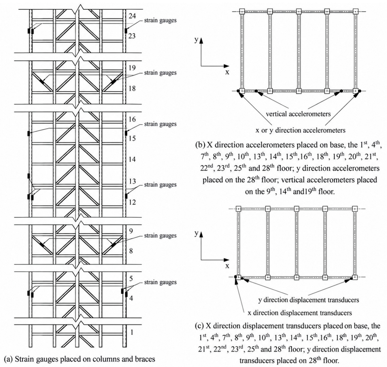
The shaking-table specimen comprised 28 physical model levels with a total height of 5.04 m, a level spacing of 0.18 m, and outrigger/belt-truss levels at model stories 9 and 19. It represented the 56-story steel core–outrigger prototype described in Ref. [9] at a geometric length scale of 1/40. The model height corresponds to a prototype height of 201.6 m, consistent with 56 nominal prototype stories of 3.6 m; each 0.18 m model interval therefore represents the overall height of two prototype stories under the simplified planar idealization. The tested structural members were fabricated mainly from red copper. Two planar frames were connected by linkages, and floor slabs and 180 kg of additional mass were included (Figure 1 and Figure 2). The experiments were conducted on the Tongji University shaking table. Nineteen horizontal acceleration positions were available for transient-feature analysis, with a subset of ten sensors used for first-mode tracking. The intact Case 1 response was sampled at 512 Hz. The geometric and dynamic response descriptions establish the basis of the present interpretation; further material-similitude parameters and sensor calibration specifications are discussed in Section 6.4 in relation to wider application of the results.

Seven unidirectional loading cases were applied sequentially. Cases 1 and 5 used 0.05 g white-noise inputs, giving the first three measured modal periods of (0.530, 0.159, 0.082) s and (0.533, 0.160, 0.083) s, respectively. Case 2 used the original El Centro record. The first- and second-mode-targeted El Centro motions in Cases 3 and 4 applied nominal amplification factors of 30 to the prescribed period bands 0.75T1–1.25T1 and 0.75T2–1.25T2. These resonance-focused cases produced residual deformation and local deterioration. Case 6 used the original Chi-Chi record. Case 7 used a first-mode-targeted Chi-Chi input with a nominal amplification factor of 5 within the 0.9T1–1.1T1 period band and ultimately produced exterior-column compression failure near model level 13 and lateral collapse. The input modifications were designed to examine resonance sensitivity under intensified dynamic loading. In Case 7, the nominal acceleration of 0.070 g and recorded shaking-table peak acceleration of 0.103 g differ by 47.14%. This provides a measure of the achieved peak input and motivates further comparison of target and measured spectra when assessing excitation fidelity. The initial structural condition of Case 7 included the residual effects of the preceding load cases.

Figure 1. Shaking-table test model.

Figure 1. Shaking-table test model.

Figure 2. Sensor layout of the test model.

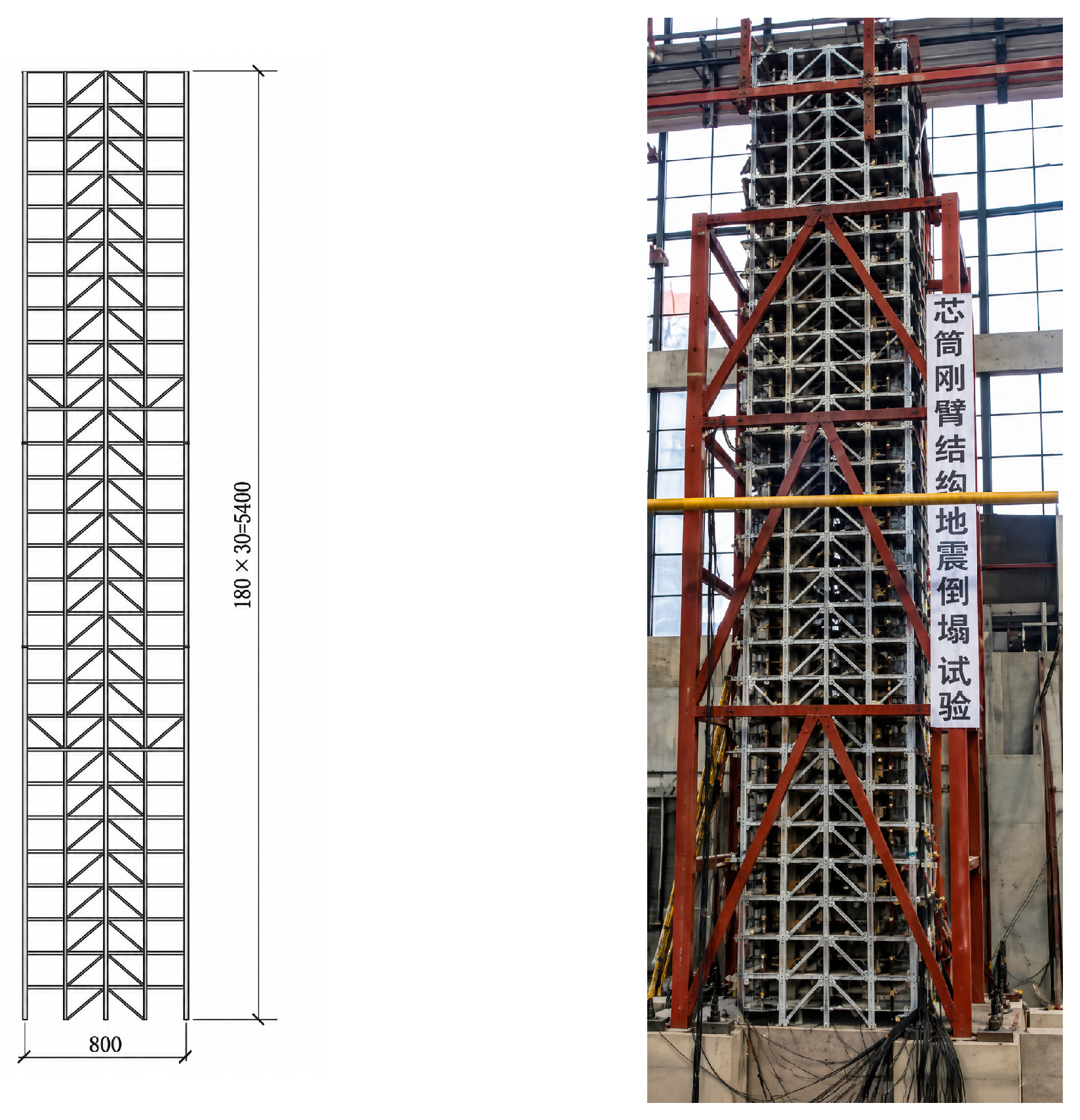
Figure 2. Sensor layout of the test model.

2.2. Evidence Chain Linking Local Buckling, Impact, and Dynamic Degradation

In Case 7, the vertical acceleration at the midspan of the 14th-level left frame beam exhibited several pronounced short-duration pulses (Figure 3). These transients are consistent with rapid local member instability, contact, and connection-related impacts. Their interpretation is strengthened by the temporal agreement with the strain measured at the 13th-level exterior column, the displacement response, and the reported physical failure observations. Impacts involving adjacent members may also contribute to the high-frequency response. The event times are compared at the time resolution of the recorded response plots; a finer evaluation of inter-channel delay would benefit from the acquisition-system timing records. The combined observations therefore provide a physically supported account of the development of local instability and impact response.

Figure 3. Impact response in Case 7. (note: ➀ Initial impact: Onset of local column instability. ➁ Secondary impact: Progressive local damage. ➂ Strong impact: Possible connection or weld damage. ➃ Further impact: Continued local instability and damage. ➄ Sensor detachment: Detachment of the 13th-floor displacement trans-ducer).

Figure 3. Impact response in Case 7. (note: ➀ Initial impact: Onset of local column instability. ➁ Secondary impact: Progressive local damage. ➂ Strong impact: Possible connection or weld damage. ➃ Further impact: Continued local instability and damage. ➄ Sensor detachment: Detachment of the 13th-floor displacement trans-ducer).

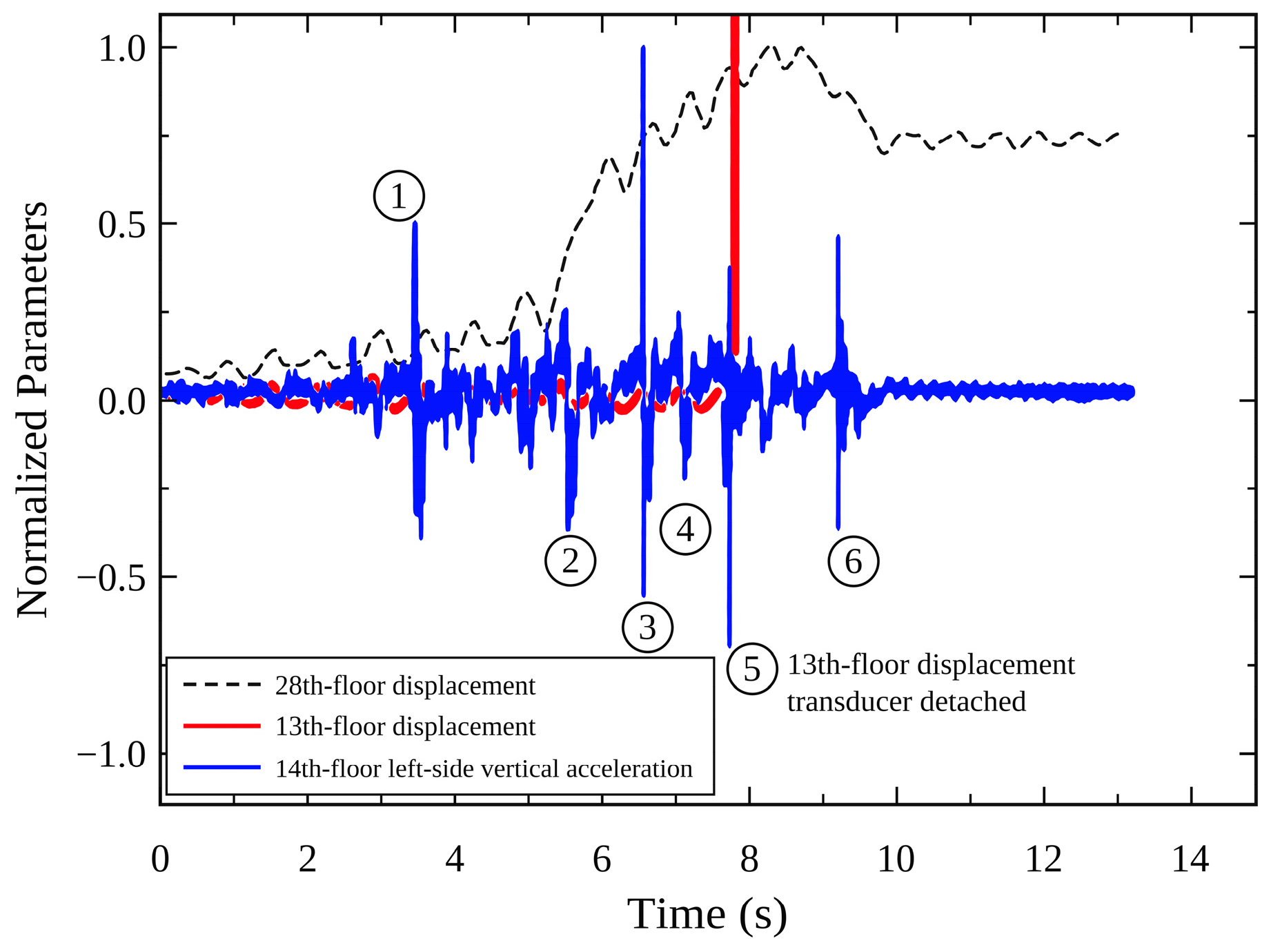
Figure 4 compares the normalized time histories of the 14th-level left-side vertical acceleration and the 13th-level left-column strain in Cases 3, 4 and 6. Although the acceleration pulses in these cases were smaller than those recorded during Case 7, pronounced transient changes corresponded in time with increases in local strain. This correspondence indicates that impact-type high-frequency responses accompanied the progressive development of local instability during the preceding excitation cases. The association becomes especially evident as deformation accumulates around the affected exterior-column region.

In Case 3, the 14th-level left-side vertical acceleration and 13th-level left-column strain changed abruptly at approximately 3.2 s. The earlier experimental investigation [9] also reported the beginning of residual roof-vertical deformation near this instant. The agreement among these measurements supports an interpretation involving local column buckling followed by contact or impact. Given the horizontal excitation and the frame geometry, additional vertical response can arise when deteriorating members interact with neighboring components. The joint strain, acceleration, and displacement observations provide stronger physical evidence for this process than the vertical-acceleration pulse alone.

Figure 4. Normalized comparison of characteristic response curves for Cases 3, 4, and 6.

Figure 4. Normalized comparison of characteristic response curves for Cases 3, 4, and 6.

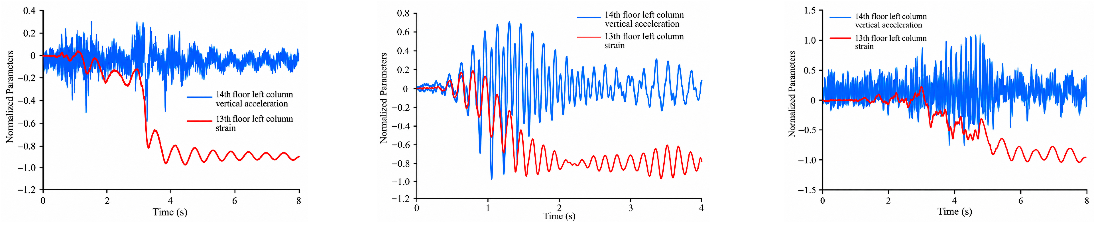
In Case 4, several abrupt changes in vertical acceleration occurred between 0.9 and 1.4 s, while the strain in the 13th-story left column increased in stages. This suggests that local buckling of the column evolved from an initial abrupt event into a progressive process. Compared with Case 3, strain growth in Case 4 was more distributed in time, suggesting that the onset of instability may be abrupt, whereas subsequent buckling propagation is relatively gradual.

Case 6 similarly exhibited repeated increases in vertical acceleration and accumulated strain between 3.3 and 4.8 s, indicating continued development of local buckling in the 13th-story left column. Comparison of Cases 3, 4, and 6 shows that local buckling can generate impact-type responses, but whether it produces a discernible change in the overall dominant dynamic characteristics depends on the severity of damage.

The horizontal displacement response of the 13th-level left column in Case 7 was analyzed over two intervals surrounding the first pronounced impact (Figure 5). The short-time dominant period increased from 0.571 s during 1–3 s to 0.666 s during 4–5 s. This corresponds to an increase of 0.095 s (16.64%) and a reduction of approximately 14.26% in the reciprocal spectral frequency. The marked lengthening of the dominant response time scale coincides with the development of local damage and lies beyond the initial first-mode resonance band. Because the response is strongly nonstationary during this stage, the period values are interpreted as dominant short-time spectral characteristics. Their evolution offers a complementary dynamic indicator of the transition documented by the local strain and transient acceleration measurements.

Figure 5. Power spectra of the horizontal displacement time history of the 13th-story left column in Case 7.

Figure 5. Power spectra of the horizontal displacement time history of the 13th-story left column in Case 7.

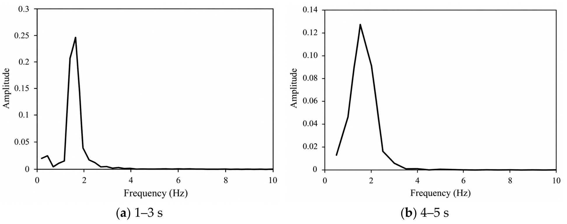
For comparison, the short-time dominant period in Case 3 remained approximately 0.665 s before and after the impact at 3.2 s (Figure 6), with no resolvable change. Similar results were obtained for Cases 4 and 6.

Figure 6. Power spectra of the horizontal displacement time history of the 13th-story left column in Case 3.

Figure 6. Power spectra of the horizontal displacement time history of the 13th-story left column in Case 3.

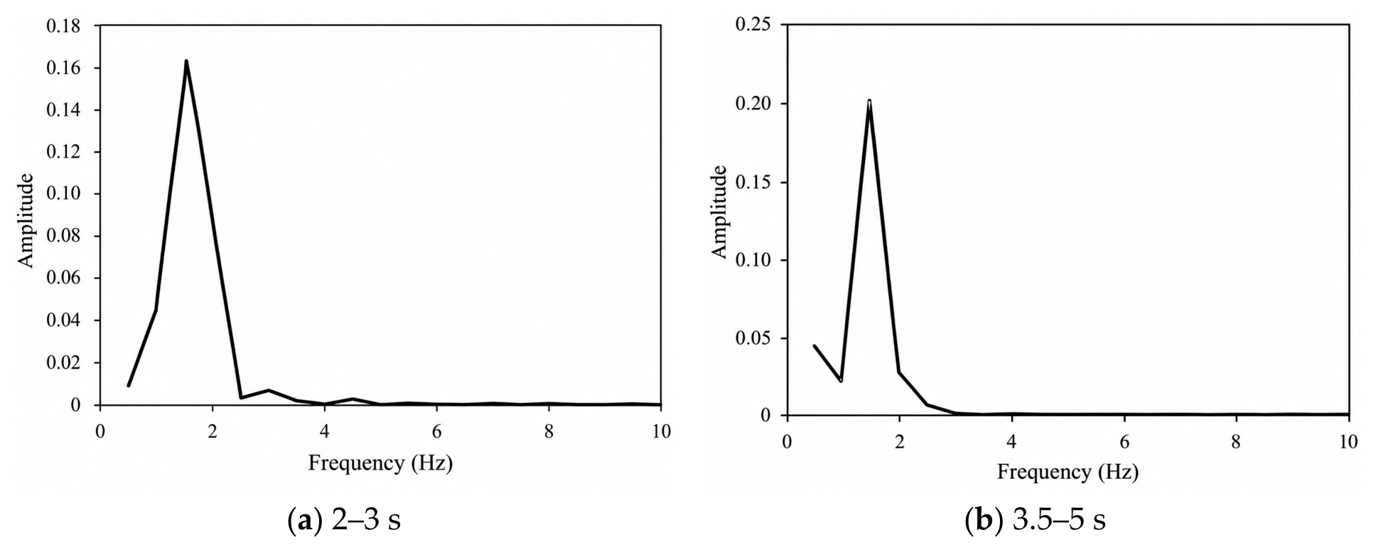
Thus, although local buckling in the earlier cases generated impact-type acceleration changes, its effect on the overall dominant dynamic characteristics remained limited. In Case 7, as local damage developed further, impact events coincided with a lengthening of the dominant period. Multi-point WT-ICA and sliding-window modal tracking are used below to further characterize the spatiotemporal evolution of damage.

3. Event-Guided Joint Damage–Modal Identification Method

3.1. Overall Analysis Framework and Underlying Assumptions

The proposed event-guided interpretation has three complementary levels. At the event level, wavelet-transform-assisted independent component analysis (WT-ICA) examines 19 horizontal acceleration responses to identify transient-feature times and sensor-level concentration zones. At the state level, ten selected acceleration responses provide short-window estimates of the dominant first-mode-like behavior, while synchrosqueezed wavelet analysis supplements the frequency description. At the validation level, local strain, beam-vertical acceleration, and the valid displacement measurements are examined on the same test timeline. Cross-comparison of these measurement types strengthens the interpretation of the local-to-global response sequence and helps identify intervals where rapid structural changes affect modal estimates.

Interpretation of the results follows three conditions. First, the wavelet/ICA component amplitude depends on decomposition settings and the indeterminacy of ICA scaling; transient timing and the relative spatial response pattern are consequently emphasized. Second, the modal meaning of the Fast-ICA mixing matrix relies on approximate linearity and separable dominant components within an analysis window. Third, the modal assurance criterion (MAC) describes mode-vector similarity and is interpreted in conjunction with the evolving strain, acceleration, and displacement responses. The signal distribution vector (SDV) provides a spatial concentration measure at instrumented positions, with the resolution governed by sensor spacing. Accordingly, the proposed damage chronology is supported by the agreement of multiple measured response quantities in time and space.

3.2. Fundamentals of Fast-ICA and Output-Only Modal Identification

Let the vector x(t) contain m measured responses generated by the linear superposition of latent source signals s(t) through an unknown mixing matrix A, as expressed in Equation (1). Without prior knowledge of A or s(t), ICA estimates an unmixing matrix W using the non-Gaussianity and statistical independence of the source signals. Fast-ICA typically estimates W by maximizing non-Gaussianity, often through an approximation to negentropy; the basic algorithm and comparisons of objective functions and optimization strategies are available in Refs. [14,19]. In each analysis interval, centering and whitening remove the mean and decorrelate the channel covariance before estimation of independent coordinates. ICA solutions are intrinsically ambiguous in component ordering, sign, and overall amplitude; consequently, component matching and consistent normalization are prerequisites for comparing different windows.

$$x(t)=As(t)={\displaystyle \sum _{i=1}^n{a}_i}{s}_i(t)$$

(1)

The estimated independent-source coordinates are obtained from y(t) = W x(t). In a linear, lightly damped system, the structural-response mixing matrix is related to the modal-shape matrix when modal coordinates have sufficiently separable statistical characteristics [15,16,17]. This correspondence motivates the use of Fast-ICA for the dominant response component during locally stable stages. During rapid damage evolution, local contact events and changes in effective modal participation alter the source-separation conditions, and the resulting mixing vectors are interpreted with reference to the transient event record and physical observations. These considerations guide the choice of a representative first-mode-like component in each window.

3.3. WT-ICA Detection and Localization of Damage Events

Wavelet-transform-assisted independent component analysis (WT-ICA) is employed following Yang and Nagarajaiah [24]; WT denotes wavelet transform. The discrete wavelet transform (DWT) decomposes each response into multiscale detail signals to enhance short-lived changes. Fast-ICA then extracts components with distinctive temporal statistics, and the corresponding mixing vectors characterize the relative response concentration across the measurement positions. Candidate event times and spatial zones are interpreted together with independent experimental observations.

(1) DWT preprocessing: Multiscale decomposition is applied to the m sensor responses. High-frequency detail components containing local abrupt-change information are retained, and the m components at the same scale are assembled into the observation matrix. At each retained wavelet scale, the same sample alignment is maintained across channels; differing scale-dependent noise and pulse amplification restrict direct comparison of feature amplitudes across scales.

(2) Candidate-feature selection: Fast-ICA is applied to the high-frequency multichannel signal matrix to obtain independent components. Four feature independent components (FICs) are emphasized after examination of pulse prominence relative to component background levels, concentration of the corresponding SDVs, distinction between their dominant event patterns, and consistency with independent physical observations. These criteria combine transient clarity, spatial information, and engineering interpretation. For further quantitative sensitivity studies, Section 3.3 also introduces scale-invariant diagnostics for pulse prominence and spatial concentration.

(3) Timing and spatial interpretation: The local maxima of each selected FIC provide approximate event times. The associated SDV identifies the sensor positions at which a feature is most pronounced. A reproducible quantitative audit may use two dimensionless indices: $P = \left[max\right|s|- median|s\left|\right]/[1.4826MAD\left(\right|s\left|\right) + epsilon]$ for robust pulse prominence and $C = \left[sumoft\mathrm{h}et\mathrm{h}reelargest\right|a_i{|}^2]/[su{m}_i\left|a_i{|}^2\right]$ for concentration of the corresponding ICA mixing vector a. Here epsilon is a small positive regularizer, and consistent component matching is used to address ICA permutation and sign indeterminacy. These descriptors offer a basis for future threshold and initialization-sensitivity studies. In the present experiment, the localization of exterior-column buckling at the 13th level is further supported by local strain and observed failure, giving a physically informed interpretation of the sensor-level response pattern.

3.4. Event-Guided Sliding-Window Modal Tracking and Reliability Criteria

After damage-event localization, modal identification is performed over local time windows. A frozen-time approximation is adopted for each window: if the structural parameters vary relatively slowly within the window, the response can be expanded as in Equation (2), with the structural response, mode-shape matrix, and modal coordinates corresponding to the observed signals, mixing matrix, and independent sources in the ICA model, respectively. A sliding step of 0.1 s is used to improve the temporal resolution of state changes.

$$x(\tau ,t)=\mathbf{\Phi }(\tau )q(\tau ,t)$$

(2)

For a lightly damped, approximately linear structural response, modal coordinates may possess sufficiently distinct statistical properties for identification through Fast-ICA [15,16,17]. A short analysis window represents the response over a locally evolving state, and changes in stiffness, contact conditions, or mode participation can influence the separated components. Closely spaced modes, measurement noise, and the available number of oscillation cycles also contribute to identification stability. The present analysis therefore follows the dominant first-mode-like component in intervals with interpretable narrowband behavior and examines the correspondence between modal changes and independently observed transient events. The damping ratios are outside the parameters evaluated here.

To balance statistical stability with the temporal localization of rapid response changes, the event-guided workflow combines coarse segmentation and fixed-window tracking. Prominent WT-ICA events identify candidate state intervals, and modal extraction is then performed in successive 6 s windows advanced by 0.1 s. The narrowband character and continuity of the estimated first-mode component are assessed with reference to event position within the window and to the independent measurements. Windows that contain strong impulses or rapidly changing response are interpreted with additional care because the local frozen-time approximation becomes less representative. The procedure thus provides a qualified description of the evolving dominant response.

The modal-tracking workflow comprises five steps: (1) select the ten-channel acceleration record, center and whiten the responses, and divide them into overlapping windows; (2) apply Fast-ICA and examine independent-component spectra to select the dominant narrowband first-mode candidate; (3) resolve component order, sign, and scalar indeterminacies to maintain consistent mode matching across windows; (4) compare mode-shape similarity using MAC together with spectral and physical consistency; and (5) apply synchrosqueezed wavelet analysis to a sufficiently separated oscillatory component to extract its dominant frequency trajectory. The intact Case 1 assessment uses MAC > 0.98 as a reference-shape criterion. For future repeated-initialization assessments in the collapse stage, accepted-run proportions, pairwise modal similarity, and frequency dispersion offer complementary measures of robustness. The Case 7 plots are interpreted in relation to the evolving spectra, event chronology, and measured deformation.

4. Damage-Event Identification: Temporal Evolution and Spatial Migration

4.1. Collapse-Case Data and Response Characteristics

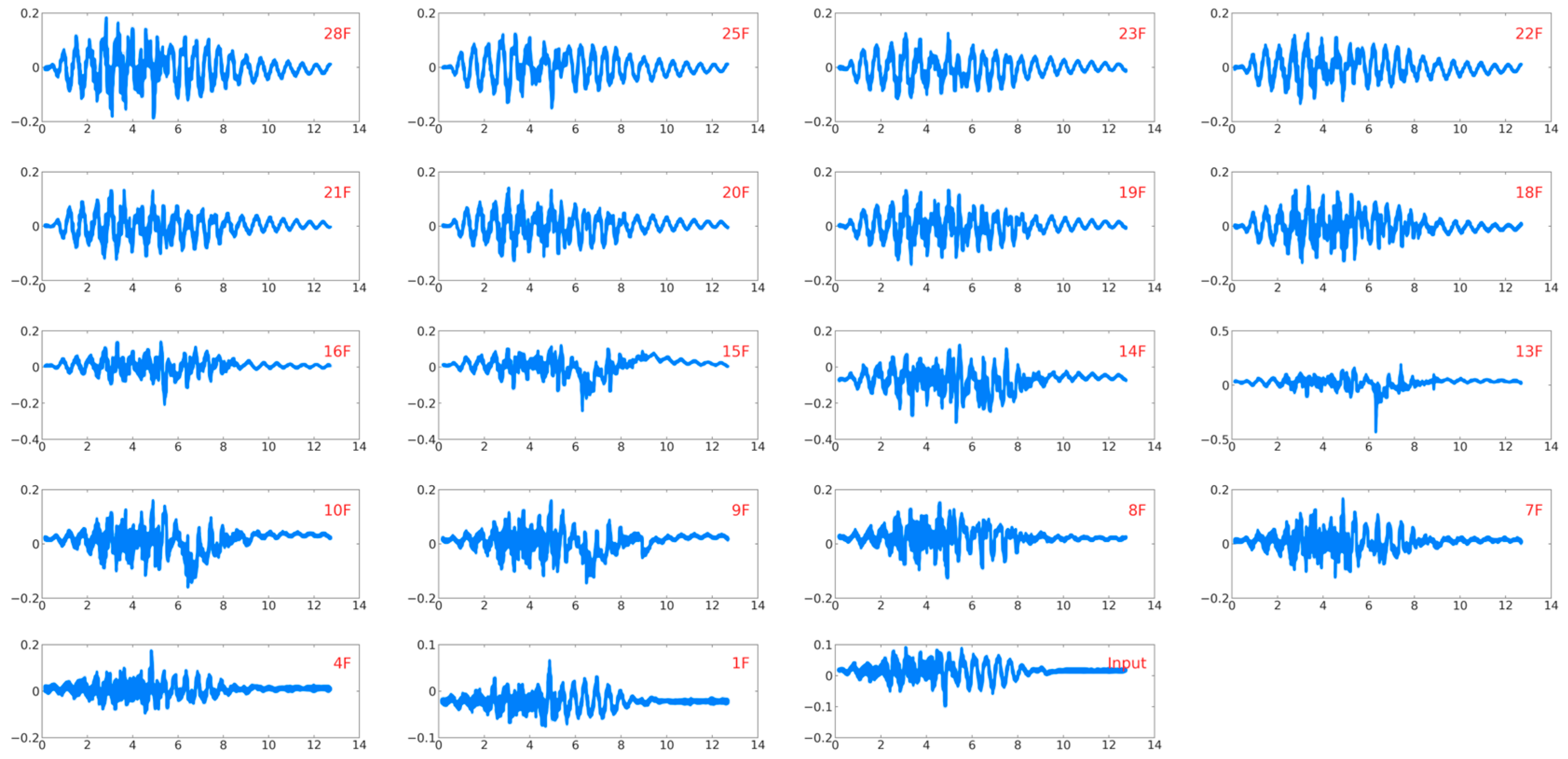
For Case 7, the nominal first-mode-targeted Chi-Chi input had a PGA of 0.070 g, while the measured shaking-table PGA was 0.103 g. Horizontal acceleration was recorded at 19 locations: the column base and model levels 1, 4, 7–10, 13–16, 18–23, 25 and 28 (Figure 7). The nominal inter-level height is 0.18 m, so a three-level gap corresponds to 0.54 m on the model; the instrumentation is denser, at 0.18 m level increments, near model levels 13–16. These values describe measurement spacing, not localization error. A peak SDV contribution at one of the densely measured levels does not exclude a shared event or transmission from adjacent members.

Figure 7. Horizontal acceleration responses in Case 7 (Chi-Chi first-mode resonant input).

Figure 7. Horizontal acceleration responses in Case 7 (Chi-Chi first-mode resonant input).

4.2. WT-ICA Parameter Settings and Feature Separation

The WT-ICA processing for Case 7 was performed as follows.

(1) DWT preprocessing: The 19 horizontal acceleration responses were decomposed using a four-level db10 wavelet transform. High-frequency detail components containing prominent pulse information were selected to form a 19-dimensional observation matrix (Figure 8). Because the db10 wavelet and the number of decomposition levels affect pulse amplitude and scale allocation, they are treated here as feature-extraction parameters; FIC amplitude is not interpreted as an absolute measure of damage. Reported pulse times refer to the instrumented record; changing the wavelet basis or decomposition levels may shift pulse prominence and warrants sensitivity assessment before general deployment.

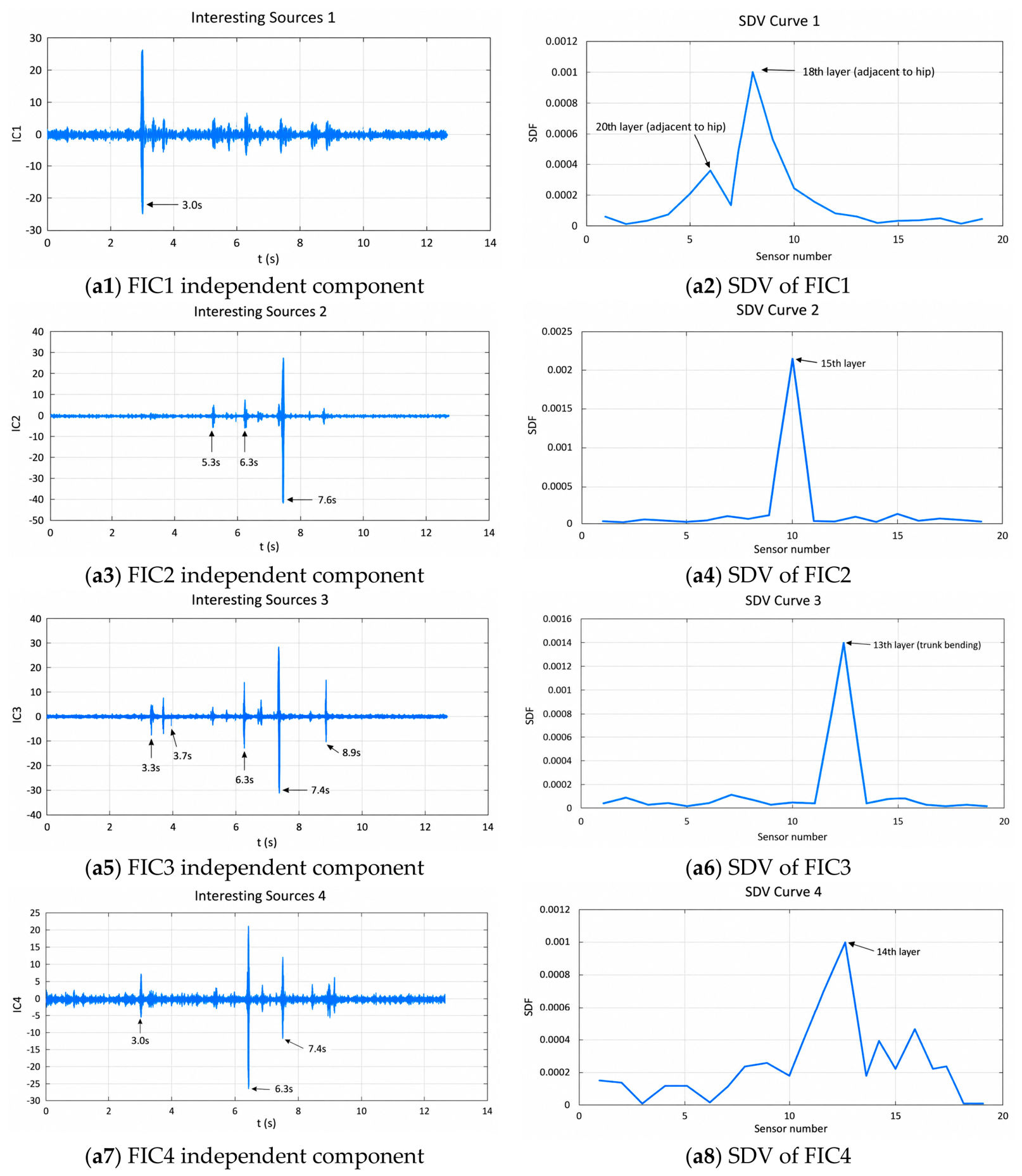
(2) Fast-ICA feature separation: Application of Fast-ICA to the 19-channel high-frequency matrix produced 19 independent components. Four FICs were selected for detailed discussion based on relatively prominent pulses, spatial concentration of their SDVs, distinct event patterns, and consistency with the measured strain and displacement responses (Figure 9 and Figure 10). Components with diffuse fluctuations or overlapping event patterns were given less weight in constructing the physical chronology. The dimensionless pulse and SDV measures introduced in Section 3.3 provide a complementary framework for future sensitivity testing of this selection.

Figure 8. High-frequency detail signals obtained by DWT for Case 7.

Figure 8. High-frequency detail signals obtained by DWT for Case 7.

Figure 9. Fast-ICA independent components of the high-frequency responses in Case 7.

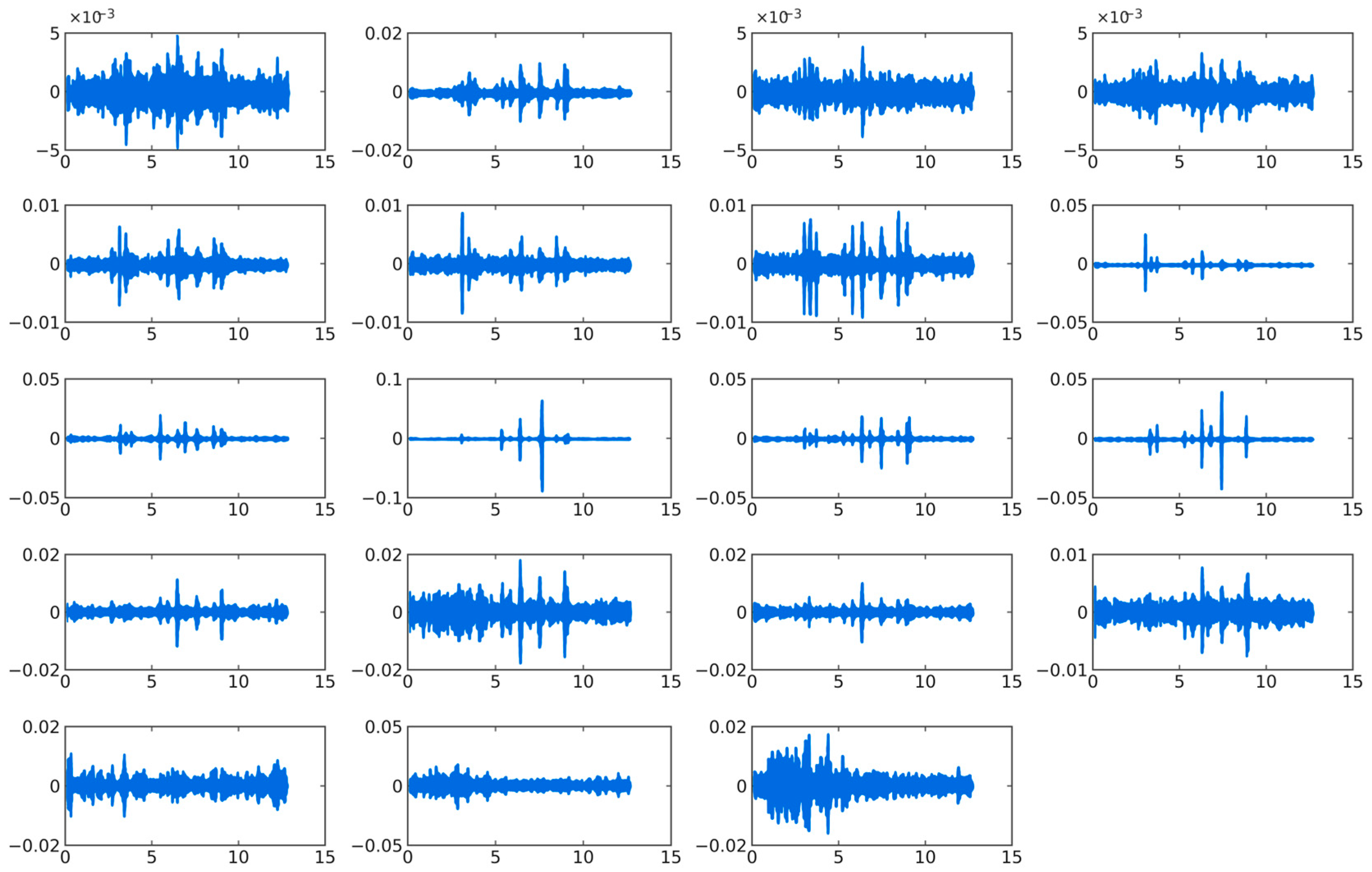
Figure 9. Fast-ICA independent components of the high-frequency responses in Case 7.

Figure 10. Feature independent components and normalized SDVs for Case 7.

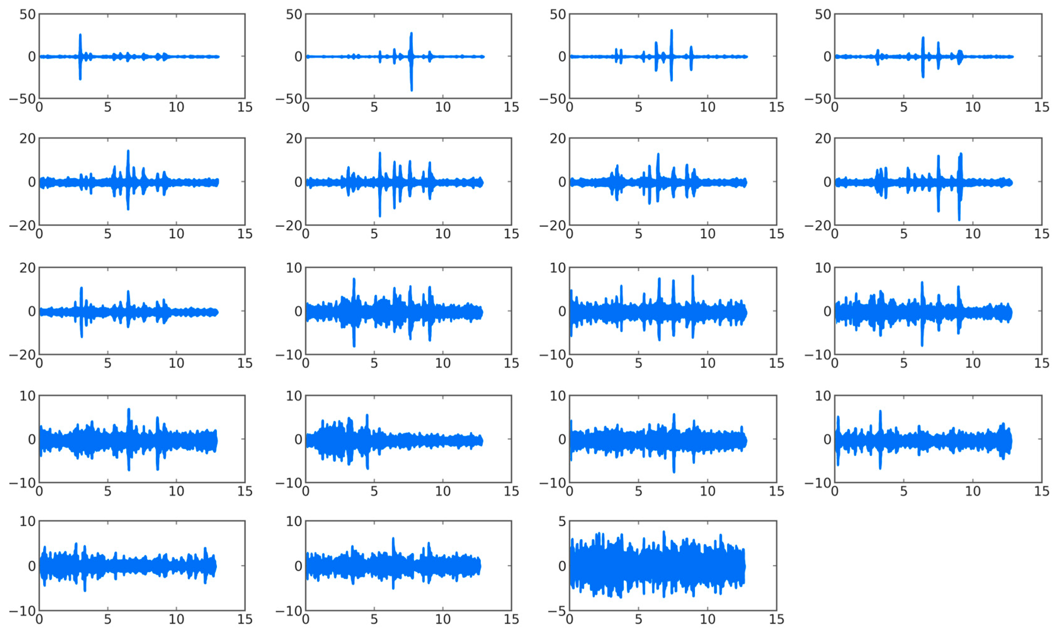
Figure 10. Feature independent components and normalized SDVs for Case 7.

4.3. Damage-Event Chronology and Critical Vulnerable Region

The event chronology combines the pulse times of the four selected FICs with the spatial distribution of their SDVs and the independent strain/impact observations introduced in Section 2. A damage-related event is interpreted through agreement among the measured response quantities. SDV maxima identify concentrated response zones on the available sensor grid, while the local strain response and documented member instability provide the specific attribution to the 13th-level exterior-column region. This combined interpretation is used throughout the event analysis.

FIC1 exhibited its first pronounced pulse at approximately 3.0 s, with SDV energy concentrated in stories adjacent to the upper outrigger, consistent with the earliest detectable local state-change feature in the measured upper-outrigger-adjacent zone.

FIC2 contained persistent pulses from 5.3 to 7.6 s, with the spatial response concentrated mainly at the 15th story, indicating a localized response feature centered on the 15th-story sensor, not a uniquely identified failure of that story during the developing collapse.

FIC3 contained the largest number of damage pulses: pronounced events repeatedly occurred near the 13th story from 3.3 to 8.9 s. Together with the strain–vertical-acceleration evidence in Section 2.2, the event near 3.3 s is temporally and spatially consistent with local buckling of the 13th-story exterior column and a strong impact. The dominant period subsequently lengthened from 0.571 s to 0.666 s and shifted outside the initial first-mode resonance band. Based on the observed test phenomena, strong pulses near 6.3 and 7.4 s were reported near observed connection/weld-point failures of the 13th-story column.

FIC4 contained persistent pulses from 3.0 to 7.4 s, with the spatial distribution concentrated mainly at the 14th story, adjacent in the instrumented grid to the local strain-evidenced buckling region at the 13th story.

Together, the four selected FICs delineate a progression of transient response features. The first prominent feature appears near the upper outrigger around 3.0 s, followed by increasingly concentrated activity around levels 13–15 and a strong event cluster around 7.4–7.6 s. This sequence provides event anchors for the subsequent sliding-window modal analysis. The physical failure observation and the 13th-level strain response strengthen the attribution of the most vulnerable local region within the measured 13th–15th level zone.

5. Time-Varying Modal Tracking: From Local Damage to Overall Rotation

Section 4 identified when and where damage was concentrated. This section further examines how these local damage events altered the dominant dynamic behavior of the structure and evolved into overall rotation. Because the collapse record is only 12.64 s long and contains densely spaced abrupt events, intact white-noise data are first used to calibrate the repeatability of Fast-ICA identification for different window lengths. The WT-ICA events are then used to constrain interpretation of the sliding-window results during collapse.

5.1. Reliability Assessment of Modal Identification and Window-Length Calibration

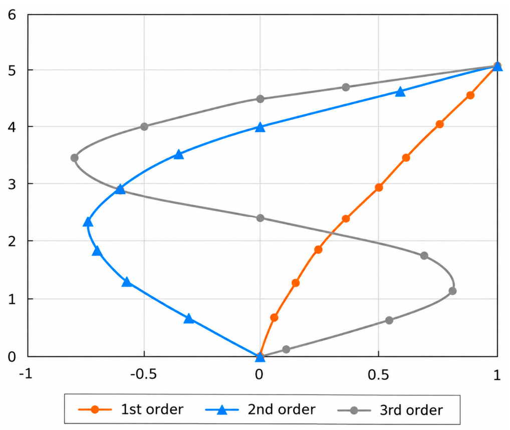
Figure 11 presents the first three reference mode shapes from the finite element model. The white-noise response from Case 1 is used to assess the modal-identification capability of Fast-ICA and to examine the effects of sensor number and window length. For the intact structure, the modal assurance criterion (MAC) is used to quantify the shape similarity between the identified mode shape and the numerical reference mode shape [34], as defined in Equation (3).

$${\mathrm{MAC}}_i={\displaystyle \frac{{\left({\varphi }_i^{\mathrm{T}}{\overline{\varphi }}_i\right)}^2}{\left({\varphi }_i^{\mathrm{T}}{\varphi }_i\right)\left({\overline{\varphi }}_i^{\mathrm{T}}{\overline{\varphi }}_i\right)}}$$

(3)

Here φ_r and φ_i denote the reference and ICA-identified mode-shape vectors, respectively, as in Equation (3). MAC ranges from zero to one and measures similarity between two modal vectors. The operational criterion MAC > 0.98 was adopted for repeated identification of the intact Case 1 reference. For any nonzero scalar factors a and b, MAC(a φ_r, b φ_i) = MAC(φ_r, φ_i). Consequently, roof and 13th-level normalization of a given estimated vector yield the same MAC value. Interpretation of changes between estimated mode shapes additionally considers the sampling positions, component matching, and response spectra.

Figure 11. First three mode shapes obtained from the numerical model.

Figure 11. First three mode shapes obtained from the numerical model.

A rectangular analysis window is implemented by direct segmentation with a 0.1 s sliding step. To evaluate the influence of random Fast-ICA initialization, the intact-reference study reported 50 repeated calculations at each selected window length. Table 1 summarizes the corresponding success counts. The collapse-stage tracking uses the representative narrowband first-mode estimates shown in Figures 17–19. Their interpretation is guided by spectral quality, event placement within the window, and the measured physical response. Section 6.4 describes the additional ensemble statistics that would strengthen a subsequent repeatability assessment for the adopted 6 s window.

The Case 1 response has a total duration of 106.76 s and a sampling frequency of 512 Hz. Using [10 s, 35 s] as an example, Figure 12 compares first-mode identification for three sensor configurations. Ten uniformly selected horizontal acceleration measurements produced a first-mode shape close to those obtained with denser sensor layouts while reducing computational cost. This 10-sensor configuration is therefore used for subsequent modal tracking, whereas all 19 measurements are retained for damage localization to preserve spatial resolution.

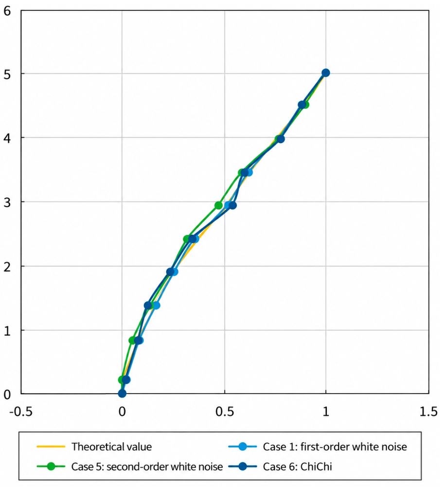
Figure 13 compares first-mode shapes identified from the Case 1 and Case 5 white-noise responses and the Case 6 original Chi-Chi response. The dominant extracted first-mode frequency is approximately 1.88 Hz. The measured first periods in Cases 1 and 5 were 0.530 and 0.533 s, a change of only 0.57%. This supports the limited change in the global low-amplitude first-mode metric in those checks; it cannot rule out the residual column deformation produced in earlier resonant load cases. Thus, the Case 7 interval before its first prominent pulse is described as the pre-collapse baseline of an already tested and locally damaged specimen, not a fresh intact state.

Case 7 has a response duration of 12.64 s and contains several prominent transient events. The evolving structural state is therefore examined through short-window estimates. Short windows improve temporal localization but reduce the amount of information available for source separation; longer windows offer greater statistical stability but may combine several stages of the damage process. The Case 1 calibration is used to describe this tradeoff. The 0.1 s sliding step provides a closely spaced series of estimates, while the 6 s integration interval determines their underlying response content.

Figure 12. Effect of sensor configuration on first-mode identification in Case 1.

Figure 12. Effect of sensor configuration on first-mode identification in Case 1.

Figure 13. Comparison of first-mode shapes before the collapse case.

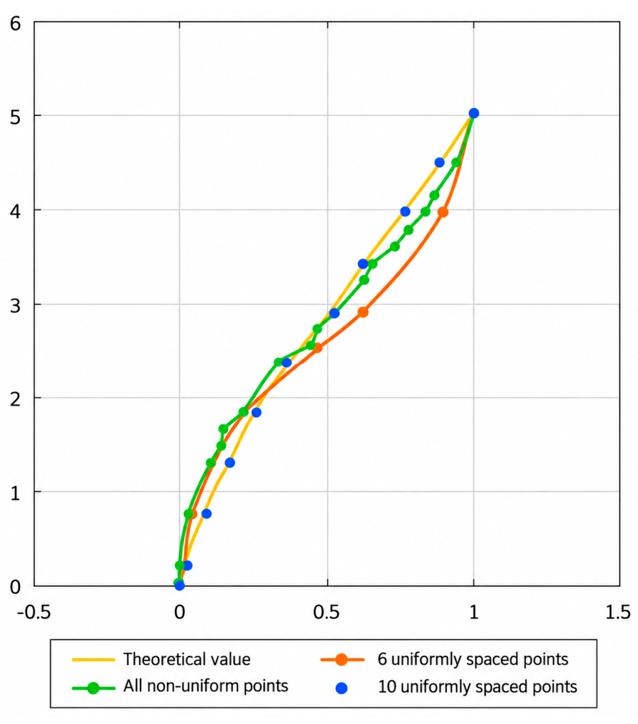
Figure 13. Comparison of first-mode shapes before the collapse case.

The intact Case 1 record provides the reference for assessing the sensitivity of modal identification to window length. The previously reported benchmark used ten acceleration channels and a starting time of 10 s, with 50 calculations for window lengths of 0.5, 1, 3, 5, 10, 15, and 90 s. The first-mode MAC > 0.98 criterion was used to summarize identification stability. The adopted 6 s window lies between the shorter intervals with lower repeatability and the longer intervals with higher repeatability. Its duration is motivated by the length of the collapse record and the importance of retaining local response information. A more extensive calibration at 6 s and neighboring lengths is discussed as an opportunity for future quantitative refinement.

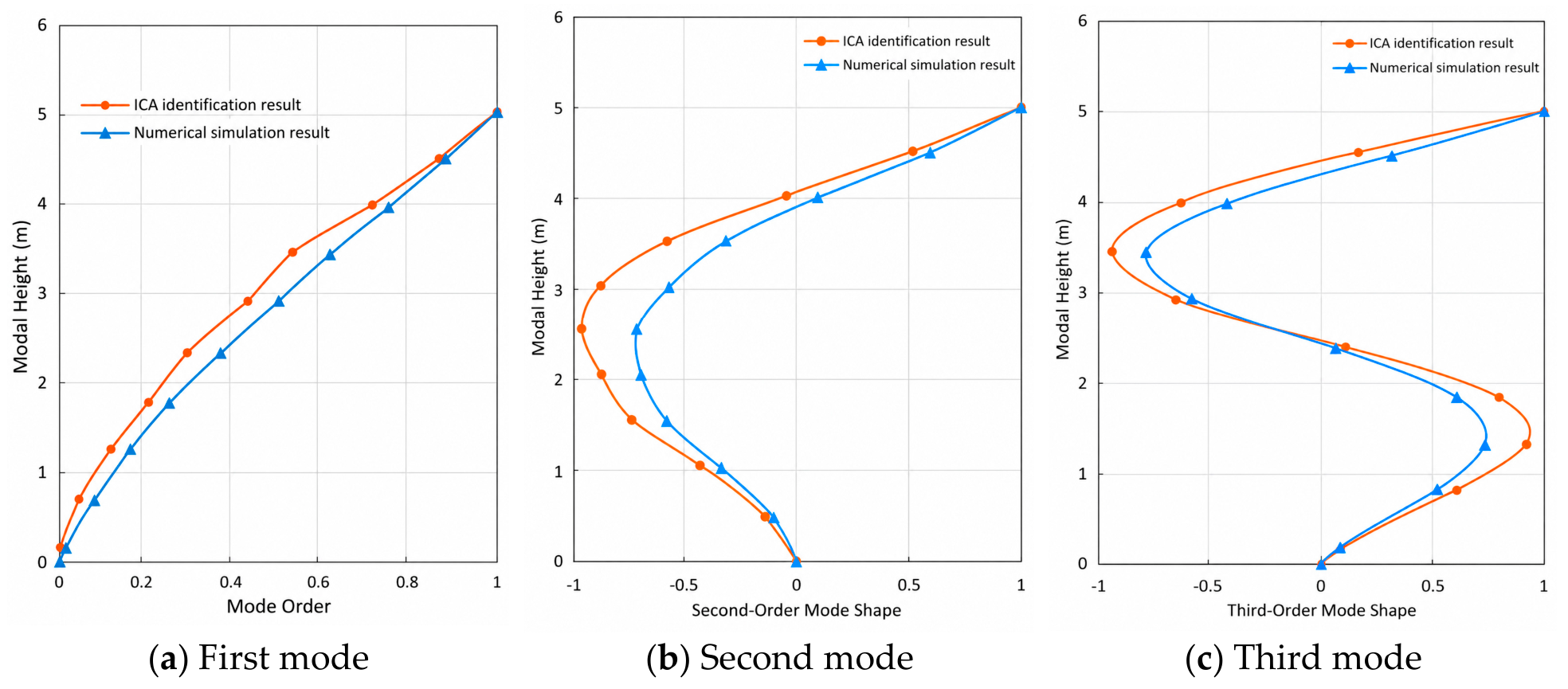
As a long-window example, Figure 14 shows the independent components and their power spectra over [10 s, 35 s], for which the components corresponding to the first three modes exhibit relatively clear narrowband peaks. Figure 15 shows that the first-mode shape in this window has MAC1 = 0.995 and satisfies the success criterion, whereas the second- and third-mode MAC values are 0.959 and 0.968, respectively, below 0.98. Because the input energy in the collapse case is concentrated mainly within the first-mode resonance band, only the first mode is tracked in the subsequent analysis.

Figure 14. Independent components and power spectra for the [10 s, 35 s] window in Case 1.

Figure 14. Independent components and power spectra for the [10 s, 35 s] window in Case 1.

Figure 15. Identified first three modes for the [10 s, 35 s] window in Case 1.

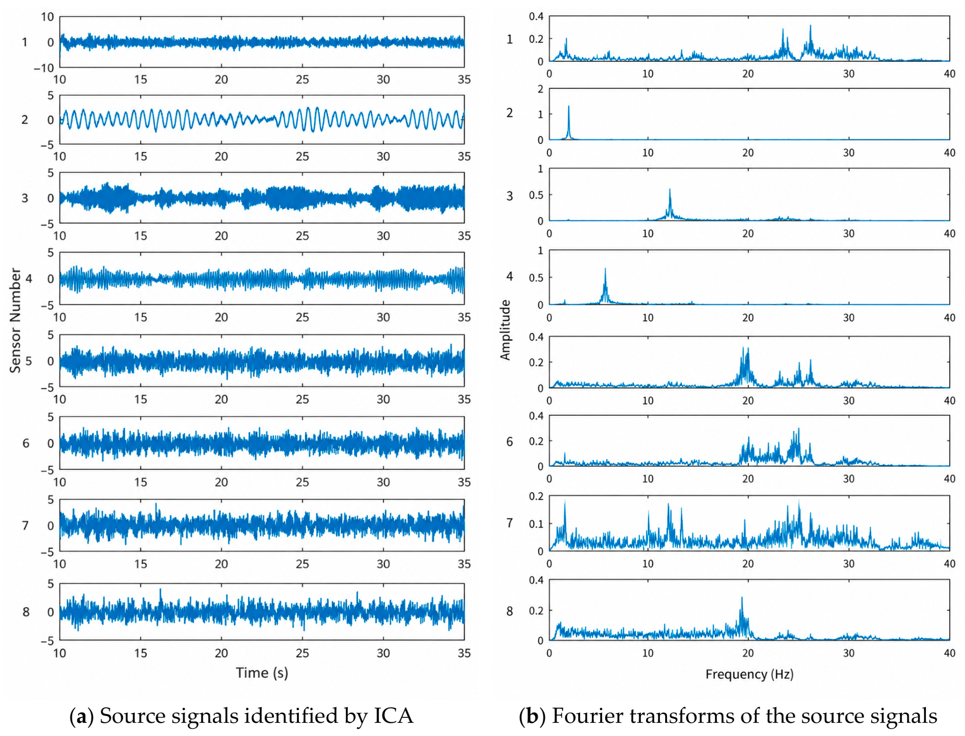
Figure 15. Identified first three modes for the [10 s, 35 s] window in Case 1.

The dominance of the first mode is specific to the first-mode resonant Chi-Chi input used in this test and does not imply that higher modes are unimportant under other earthquake inputs or damage patterns. All physical interpretations of mode-shape evolution in this study are therefore restricted to the response dominated by the first mode.

Table 1 highlights the effect of analysis-window length on the stability of the identified first mode. Successful first-mode estimates were obtained in 25/50 runs at 3 s (50%), 31/50 at 5 s (62%), and 45/50 at 10 s (90%); windows of 15 and 90 s each yielded 50/50 successes. The 0.5 and 1 s intervals yielded 0/50 and 1/50 successes. At the 512 Hz Case 1 sampling rate, a 6 s window contains 3072 samples and approximately 11.32 periods of the initial 0.530 s first mode. This combination of data length and relative temporal locality supports its use for representative tracking in the 12.64 s collapse record. The calibration also highlights the benefit of reporting repeated-run statistics together with spectral narrowband character when applying modal identification to strongly evolving responses.

A 6 s window with a 0.1 s sliding increment was therefore adopted for following the evolution of the dominant first-mode-like response through the available Case 7 record. The selected length accommodates several oscillation cycles and retains the ability to compare response stages in the compact collapse record. The resulting modal vectors are interpreted jointly with the independent event chronology and the measured structural deformation. Additional repeated-initialization experiments at 6 s and 7 s, including the dispersion of identified frequencies and modal vectors, would further quantify window-length sensitivity and are included among the prospective verification activities discussed in Section 6.4.

Table 1. Stability of first-mode identification for different window lengths under the Case 1 white-noise input (t0 = 10 s).

Window Length Δt	Time Interval	MAC1	Successful Runs (out of 50)
0.5 s	[10 s, 10.5 s]	0.913	0/50
1 s	[10 s, 11 s]	0.969	1/50
3 s	[10 s, 13 s]	0.998	25/50
5 s	[10 s, 15 s]	1.000	31/50
10 s	[10 s, 20 s]	1.000	45/50
15 s	[10 s, 25 s]	1.000	50/50
90 s	[10 s, 100 s]	1.000	50/50

Table 1. Stability of first-mode identification for different window lengths under the Case 1 white-noise input (t0 = 10 s).

Window Length Δt	Time Interval	MAC1	Successful Runs (out of 50)
0.5 s	[10 s, 10.5 s]	0.913	0/50
1 s	[10 s, 11 s]	0.969	1/50
3 s	[10 s, 13 s]	0.998	25/50
5 s	[10 s, 15 s]	1.000	31/50
10 s	[10 s, 20 s]	1.000	45/50
15 s	[10 s, 25 s]	1.000	50/50
90 s	[10 s, 100 s]	1.000	50/50

5.2. Event-Guided Two-Stage Modal Tracking

The selection of a sliding-window duration depends on the oscillatory information content and the evolution rate of the structural response. As a simple heuristic, an interval containing two cycles of the initial dominant mode provides a lower information scale, expressed by the sample-count relation in Equation (4). For robust modal extraction, longer windows may be necessary depending on excitation, noise, and modal separation. The Case 1 repeated-run benchmark in Table 1 provides an empirical basis for selecting among candidate durations for this experiment.

$$l=2{\displaystyle \frac{f_s}{f_1}}$$

Here l is the number of samples in the analysis interval, f_s is the sampling frequency, and f_1 is the initial first-mode frequency. For the measured 0.530 s first period, 6 s encompasses approximately 11.32 oscillation cycles. With a 0.1 s sliding increment, adjacent windows share 5.9 s, equivalent to 98.33% overlap. This provides a dense depiction of the progressive response and indicates the strong statistical dependence between neighboring window estimates. The first-mode interpretation is accordingly assessed using spectral separability, event chronology, and consistency with the measured global response.

Within each 6 s window, the structural response is described by an approximate frozen-time representation. Prominent WT-ICA events help identify intervals where the response may change rapidly and where the first-mode estimate requires additional scrutiny. The reliability of the separated component is assessed in conjunction with its narrowband character and continuity over the valid neighboring windows. When intense impacts enter a window, variations in modal participation and local stationarity may reduce the stability of ICA separation. Such intervals are interpreted together with independent strain and displacement measurements.

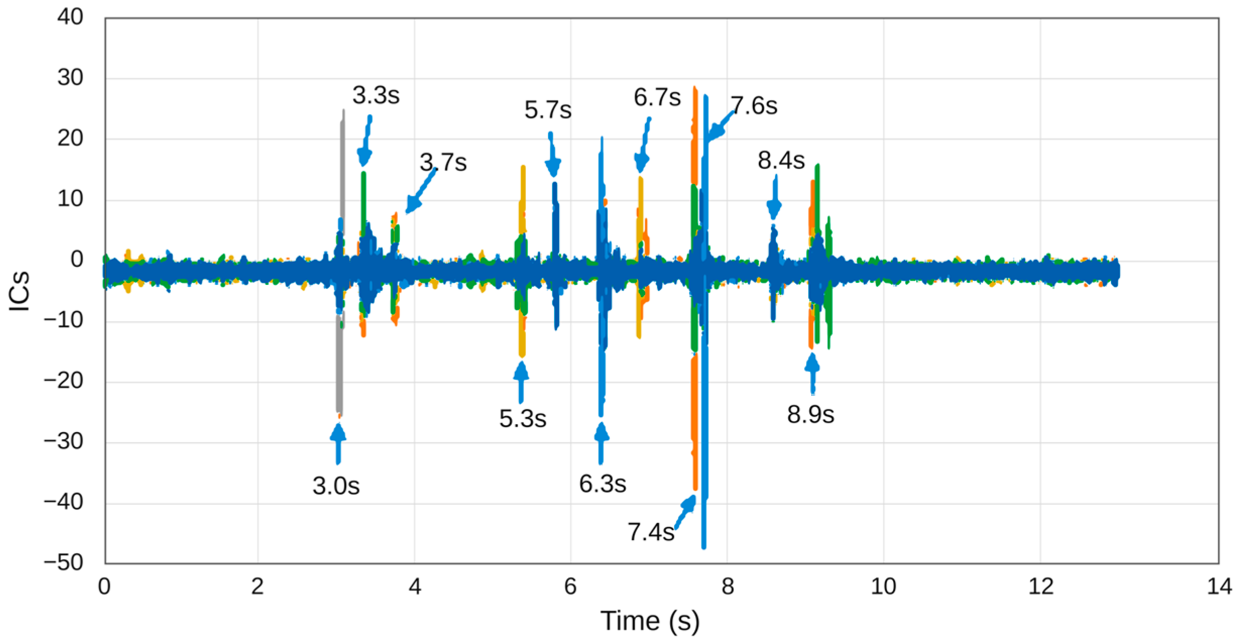
To facilitate window selection, Figure 16 overlays the principal FICs together with several ICs containing fewer pulses. Pronounced pulses occur at approximately 3.0, 3.3, 5.3, 6.3, 7.4, 7.6, and 8.9 s, with the strongest events concentrated around 7.4–7.6 s.

Figure 16. Principal damage-pulse times in the WT-ICA feature components.

Figure 16. Principal damage-pulse times in the WT-ICA feature components.

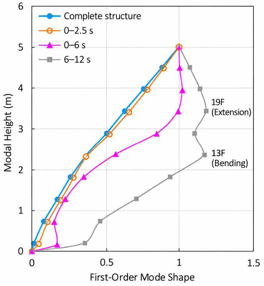
A coarse segmentation is first performed. The Case 7 record lasts 12.64 s; using the strong damage event near 6.3 s as a reference, [0, 6 s] and [6, 12 s] are analyzed separately, with the pre-damage interval [0, 2.5 s] used as the baseline (Figure 17). The first mode shape over [0, 2.5 s] is close to that of the intact structure, with MAC1 = 0.992. The middle and upper portions of the [0, 6 s] mode shape begin to depart from the baseline, while [6, 12 s] shows more pronounced shape changes at and above the 13th-story buckling region. The main changes in the dynamic characteristics therefore occur during the middle and later stages of collapse.

Figure 17. First mode shapes at different stages of Case 7.

Figure 17. First mode shapes at different stages of Case 7.

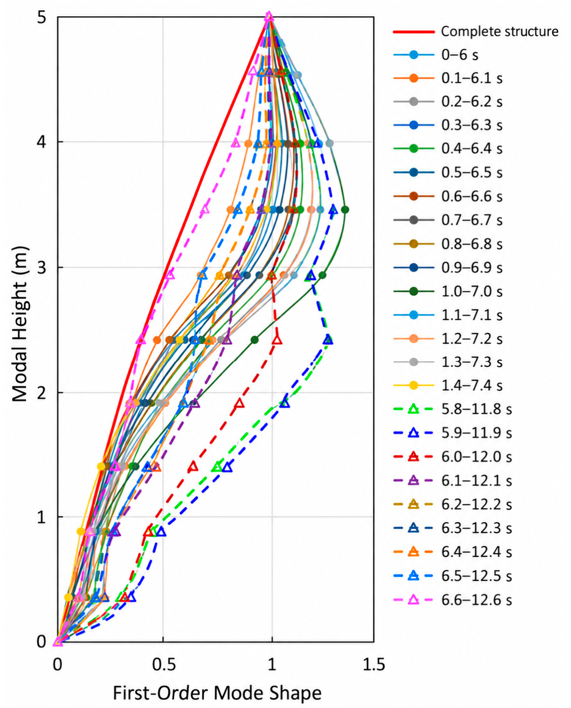
The 6 s moving-window results exhibit two groups of interpretable first-mode-like response shapes (Figure 18). The first extends from [0, 6] s to approximately [1.4, 7.4] s, with progressive shape changes near the upper outrigger. The second extends from approximately [5.8, 11.8] s to [6.6, 12.6] s, showing a more pronounced change around and above the locally damaged 13th-level region. Windows between these groups exhibit reduced narrowband separability. The strongest WT-ICA transient cluster lies around 7.4–7.6 s (Figure 16), and its position relative to the analysis window helps explain the varying clarity of the separated components. Changes in the effective modal mixture, measurement noise, and local response nonstationarity also contribute to the observed separation quality. These modal estimates are evaluated together with the independent strain and displacement results.

Figure 18. Evolution of the first mode shape identified using a 6 s sliding window.

Figure 18. Evolution of the first mode shape identified using a 6 s sliding window.

5.3. Mode-Shape Reconstruction and Normalization During Collapse

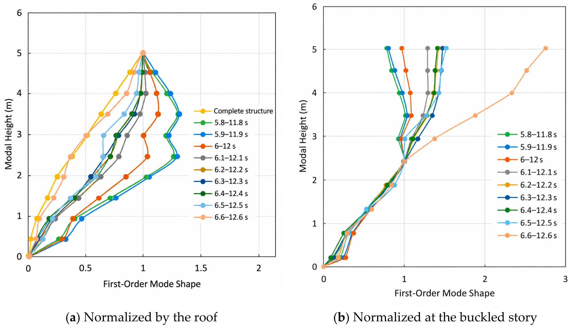
Figure 19 compares two graphical scalings of the same late-stage first-mode vectors, normalized at the roof and at the 13th model level. These representations aid visual examination of response changes around the damaged region. Since each scaling multiplies the vector by a nonzero constant, MAC and scale-invariant mode-shape descriptors have the same values under both choices. For example, the [6.6, 12.6] s vector retains its reported MAC of 0.996 relative to the intact reference. A useful quantitative extension is the dimensionless local curvature-concentration index K_H. Let the discrete modal slope over adjacent measured heights be g_j = (phi_{j + 1}-phi_j)/(z_{j + 1}-z_j); then define a curvature jump as d_j = g_{j + 1}-g_j and K_H = (sum_{j in H}|d_j|)/(sum_{all j}|d_j|), where H denotes a fixed region around the affected 13th level and the denominator is nonzero. K_H is unchanged under nonzero scalar rescaling and can quantify concentration of mode-shape variation near the vulnerable region. The experimental displacement measurements (Figure 22) independently show a growing contrast between upper and lower deformations before the local transducer detached. Together with the reported column-buckling observations, these measurements support an interpretation of progressive upper-structure movement about the locally weakened region.

Figure 19. Comparison of second-stage sliding-window first mode shapes and normalization schemes.

Figure 19. Comparison of second-stage sliding-window first mode shapes and normalization schemes.

5.4. Evolution and Physical Interpretation of Instantaneous Frequency

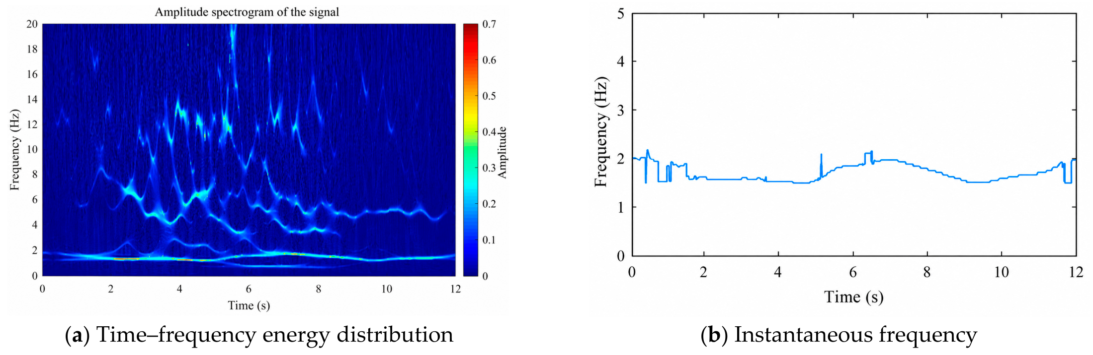
A short-window Fourier spectrum balances time localization against frequency resolution. Synchrosqueezed wavelet analysis sharpens the distribution of oscillatory energy by reassigning wavelet coefficients to estimated instantaneous-frequency locations [35]. The resulting frequency ridge provides a complementary description of the dominant component when the oscillatory response remains sufficiently separated. Its interpretation is considered together with transient events and the first-mode-like response shapes, especially near the strong impacts.

The synchrosqueezed dominant-frequency ridge in Case 7 exhibits an overall downward trend, with a brief intermediate rebound followed by a further decrease (Figure 20). The pronounced frequency reduction coincides with the period of progressively severe deformation and changes in dynamic response indicated by other response measures. The transient rebound may be associated with intermittent contact, variations in excitation amplitude, or limitations in time–frequency resolution. However, the underlying mechanism cannot be uniquely determined from the frequency trajectory alone. The observed frequency variations are therefore examined in conjunction with WT-ICA event times, strain, and displacement to describe their temporal relationship with the structural response.

Up to this point, both the damage events identified in Section 4 and the modal/frequency evolution identified in this section have been inferred from acceleration responses. To avoid a physically misleading interpretation based only on internal consistency within the same data source, Section 6 introduces independent responses, including roof displacement and interstory deformation, to examine whether 13th-story buckling, overall rotation of the upper structure, and macroscopic lateral instability follow a consistent temporal sequence.

Figure 20. Time–frequency energy distribution and instantaneous frequency of the dominant first-mode component in the collapse case.

Figure 20. Time–frequency energy distribution and instantaneous frequency of the dominant first-mode component in the collapse case.

6. Cross-Validation Using Multiple Response Sources and Reconstruction of the Lateral Collapse Mechanism

WT-ICA and sliding-window modal tracking rely on multi-point responses and can sensitively capture local damage and spatial changes in modal behavior. Because the number of sensors may be limited in practical structural monitoring, this section further examines global indicators derived only from displacement responses and evaluates whether they are temporally consistent with the local damage sequence.

6.1. Roof Displacement Response and Precursors of Global Instability

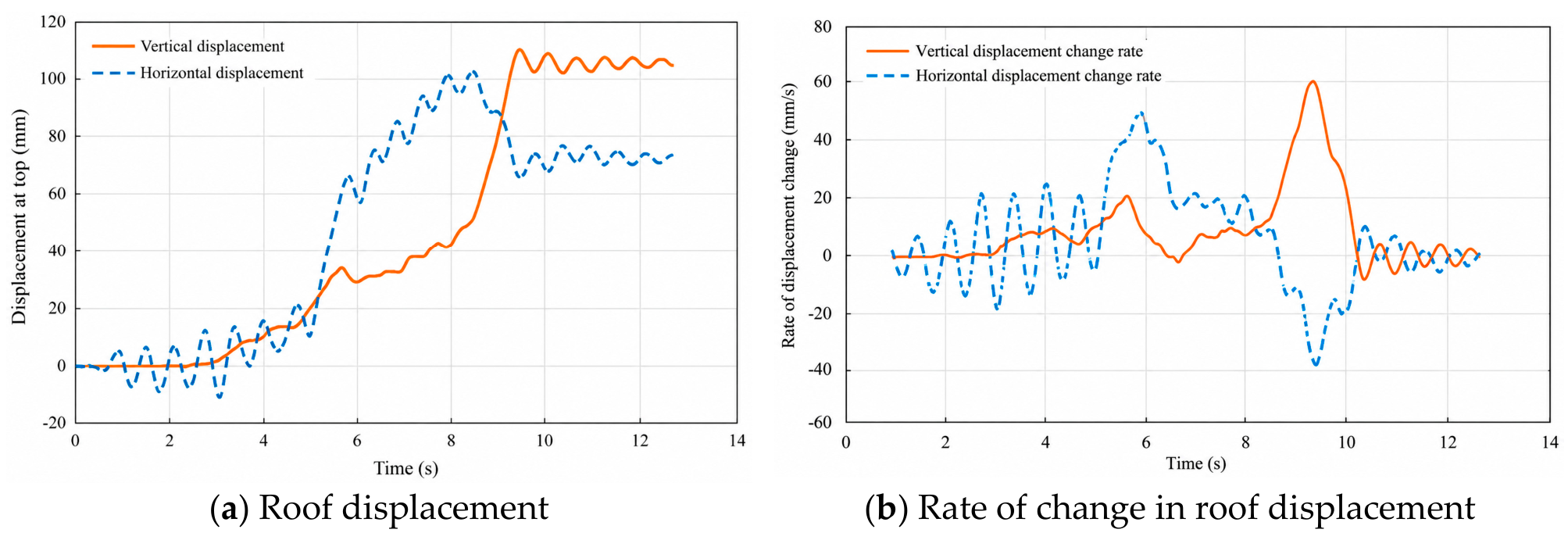
A 1 s finite difference is used to define the rate of displacement change: vd(t₀) = [x(t₀ + Δt) − x(t₀)]/Δt, with Δt = 1 s. Figure 21 shows the roof-vertical and horizontal displacements and their rates of change. Vertical displacement began to accumulate at approximately 3.0 s, underwent a second period of faster growth near 4.8 s, and increased rapidly after 8.5 s. After excitation ceased, the residual roof-vertical displacement was approximately 100 mm. Horizontal displacement developed a persistent offset to one side after 3.3 s and grew rapidly from approximately 5 s, also reaching a peak of about 100 mm. For this characteristic lateral-collapse mode, the horizontal displacement and its rate of change exhibited a clear instability trend by about 5 s, whereas catastrophic growth of vertical displacement occurred mainly after 8.5 s. The horizontal indicators were therefore more sensitive to the intermediate-story lateral failure.

Figure 21. Time histories of roof displacement and its rate of change.

Figure 21. Time histories of roof displacement and its rate of change.

6.2. Interstory Deformation and Sequence of Lateral Overturning

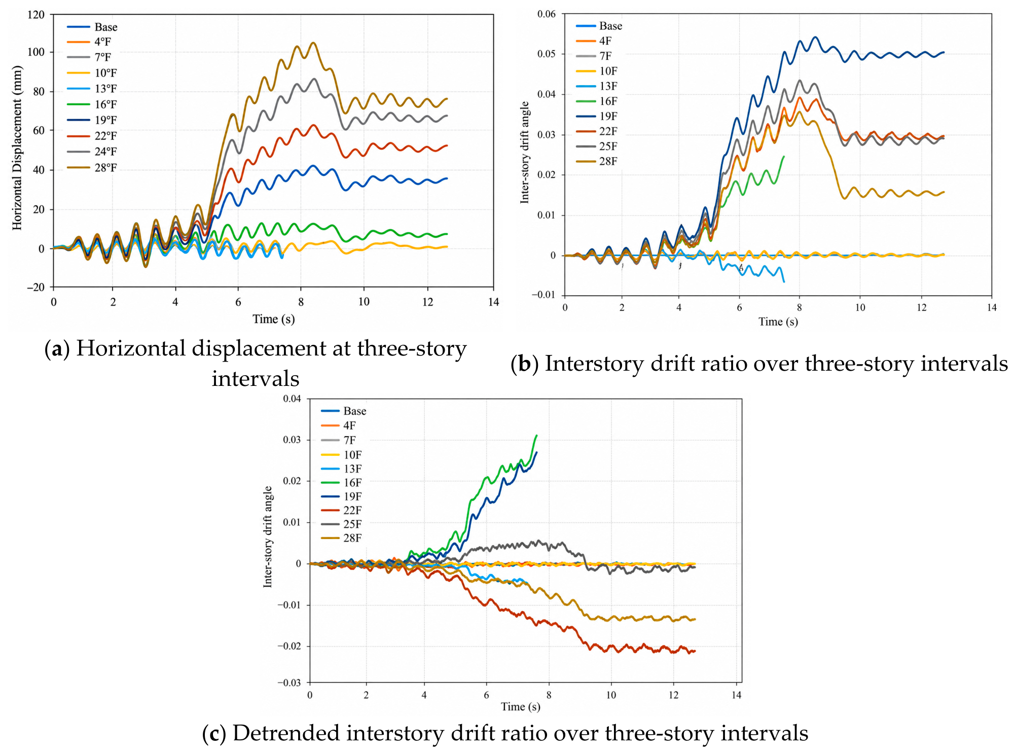
Figure 22a presents horizontal displacement at the instrumented levels, and Figure 22b,c show relative-deformation measures over the available level intervals. The 13th-level horizontal displacement transducer detached at approximately 7.4 s. The corresponding 10th–13th and 13th–16th interval drift measures are evaluated over their valid pre-detachment segments. These measurements show increasing same-direction residual offsets above the damaged region after approximately 3.3 s and a growing upper-to-lower deformation contrast from about 5.3 s. Following detachment, the valid remaining displacement channels, including the roof response, describe continuing global movement. Strong events around 7.4–7.6 s are evaluated using acceleration-derived pulses, local strain, and recorded connection damage. This distinction clarifies the measurement support for the proposed progression toward lateral instability.

The detrended inter-level deformation indices in Figure 22c further emphasize the relative accumulation of deformation above the vulnerable zone. The intervals labeled 16F and 19F exhibit particularly great changes after approximately 5.3 s, indicating an increasing difference between the upper and lower structural responses during the valid measurement interval. Together with the observed 13th-level local failure, this kinematic pattern is consistent with the formation of a rotational interface near the weakened level and the subsequent upper-structure movement.

Figure 22. Time histories of horizontal displacement, interstory drift ratio, and detrended interstory drift ratio over three-story intervals.

Figure 22. Time histories of horizontal displacement, interstory drift ratio, and detrended interstory drift ratio over three-story intervals.

6.3. Multi-Source Evidence Chain and Collapse-Stage Classification

The experimental chronology is synthesized in Table 2 using the local strain/impact evidence, WT-ICA events, sliding-window response shapes, and independent displacement histories. A candidate local state change is visible near the upper outrigger at about 3.0 s. At approximately 3.3 s, the exterior-column strain and vertical acceleration indicate pronounced local instability, accompanied by lengthening of the short-time dominant period. Upper-level relative displacement becomes more pronounced after about 5.3 s. The cluster of strong transient responses around 7.4–7.6 s coincides with reported connection damage, detachment of the 13th-level displacement transducer, and reduced reliability of local modal separation. Roof-vertical displacement grows rapidly mainly after approximately 8.5 s as collapse develops. The combined measurements support a progression in which deterioration of the local force-transfer region is followed by increasing upper-structure movement and global lateral instability. The roles of inertia, member contact, and geometric nonlinearity are considered as part of the coupled collapse process.

Table 2. Damage-evolution stages and multi-source evidence for the resonant collapse case.

Stage/Time	Local Damage Evidence	Modal/Frequency Evidence	Global Response Evidence	Mechanistic Interpretation
A: 0–3.0 s	No sustained strong FIC pulses; local responses remain generally stable.	First mode shape over [0, 2.5 s] is close to the intact baseline, MAC = 0.992.	Roof and interstory displacements remain small.	Overall state remains close to the pre-collapse baseline.
B: 3.0–3.3 s	FIC first appears near stories adjacent to the upper outrigger; at 3.3 s, exterior-column strain and impact response at the 13th story change abruptly and concurrently.	Short-time dominant period increases from 0.571 s to 0.666 s after the first strong impact.	After 3.3 s, upper-story horizontal displacements begin to shift to one side.	Local state changes precede the observed dynamic-response shift.
C: 3.3–5.3 s	Damage pulses recur near stories 13–15.	First-stage sliding-window mode shapes progressively depart from the baseline near the upper outrigger.	A second stage of roof-vertical displacement growth begins near 4.8 s; upper interstory deformation accumulates.	Continued local deterioration accompanies increasing upper-level deformation.
D: 5.3–7.4 s	Damage pulses remain concentrated at the buckled story and adjacent stories.	Mode-shape changes near the damaged region are interpreted with the displacement evidence.	Detrended interstory drift above the buckled story develops rapidly after 5.3 s.	Pre-detachment drift patterns are consistent with an emerging rotational interface.
E: 7.4–7.6 s	Intense pulses and connection damage; 13th-level displacement transducer detaches.	First-mode separation becomes difficult during the strong events.	Later movement is assessed using the valid displacement channels.	Strong transient responses coincide with reduced local modal separability.
F: >8.5 s	Damage continues to develop.	No stable local-linear parameter interpretation is assigned to the strongly nonlinear stage.	Roof-vertical displacement increases rapidly, and macroscopic lateral collapse develops.	Local load-path deterioration accompanies the development of global geometric instability.

6.4. Applicability and Limitations of the Method

The present findings are derived from a sequential series of loading cases on one 1/40-scale copper-member model. The previous tests produced local residual deformation before the final resonant collapse case, and the imposed Chi-Chi motion was deliberately amplified near the initial fundamental period. These conditions define the experimental domain of the conclusions. The instrument grid provides a nominal spacing of 0.54 m on the model and locally denser spacing of 0.18 m near levels 13–16. The reconstructed events are therefore assigned to instrumented response zones with additional support from local strain and physical failure observations. Quantitative evaluation of the FIC selection across independent initializations, story-level localization uncertainty, and the response to alternative wavelet scales would further extend the framework. The same applies to a direct 6 s/7 s repeated-identification benchmark and to frequency/shape dispersion within each Case 7 window. These assessments would be particularly valuable for determining sensitivity to the initial structural condition and the selected sensor configuration.

The stability of local modal separation depends on several interacting factors, including rapid stiffness and contact changes, modal mixing, signal-to-noise ratio, random initialization, and the effective number of locally stationary cycles. The chosen 6 s windows with a 0.1 s start increment overlap by 98.33%, giving a smoothly sampled but highly correlated sequence of modal estimates. The 13th-level displacement transducer detached at approximately 7.4 s, so subsequent kinematic interpretation relies on the remaining valid channels. Extension to other inputs can be organized using a dimensionless detuning measure $eta = |f_{i}nput - f_1|/f_1$, together with variations in bandwidth and sensor density. A future validation program could compare multi-start modal repeatability, spectral concentration and event-location agreement across these conditions. More complete calibration records for the material properties, shaking-table spectral reproduction and inter-channel timing would support detailed mechanical similitude and impact-timing studies. These extensions build on the event chronology and deformation patterns established by the present experiment.

7. Conclusions

This study provides an event-guided interpretation of the recorded collapse response of a 28-level physical model representing a 56-story steel core–outrigger prototype. It integrates transient-feature localization from 19 acceleration measurements, sliding-window dominant-response tracking, and independent strain and displacement observations. The combined results clarify the progression of local deterioration, dynamic response changes, and macroscopic instability under strong resonant excitation.

(1) The 13th-level exterior-column strain response and 14th-level beam-vertical-acceleration pulses around 3.3 s indicate developing local instability and impact-type behavior. The dominant period increased from 0.571 s to 0.666 s, corresponding to 0.095 s (16.64%) lengthening and an approximately 14.26% decrease in reciprocal frequency. This spectral change is consistent with the evolving dynamic state of the damaged structure.

(2) Four feature-independent components selected from 19 source components delineated the progression of transient events. The first detectable local state-change feature was near the upper outrigger at approximately 3.0 s. Subsequent concentrated events occurred around model levels 13–15 from about 3.3 to 8.9 s, with strong pulses near 7.4–7.6 s. Local strain and the reported member failure further identify the 13th-level exterior-column region as the critical vulnerable zone.

(3) The intact-reference Case 1 study yielded 25/50 successful first-mode identifications for 3 s windows, 31/50 for 5 s windows, and 45/50 for 10 s windows. The adopted 6 s interval contains 3072 samples at the documented 512 Hz reference rate and about 11.32 cycles of the initial first-mode response. With a 0.1 s sliding increment, neighboring windows have 98.33% overlap. These values characterize the information content and temporal sampling of the modal-tracking analysis. Intervals containing the strong 7.4–7.6 s events exhibit reduced modal-separation stability, motivating the joint interpretation with the transient and deformation measurements.

(4) The [6.6, 12.6] s modal estimate has a reported MAC of 0.996 relative to the intact reference even though substantial deformation had developed. Roof and 13th-level normalizations are scalar rescalings, leaving MAC and dimensionless modal-shape measures unchanged. A local curvature-concentration index is introduced to facilitate a quantitative study of the damaged region using the modal vectors. The directly measured pre-detachment upper-level deformation contrast provides the kinematic support for the inferred rotation of the upper structure.

(5) Upper-level relative horizontal movement became more pronounced after approximately 5.3 s, followed by a sharp rise in roof-vertical displacement mainly after approximately 8.5 s. The final residual roof-vertical displacement was about 100 mm. The valid inter-level displacement records, local strain, transient acceleration features, and observed damage together support a progressive transition from column instability toward upper-structure rotation and global lateral collapse.

References

- Ger, J.-F.; Cheng, F.Y.; Lu, L.-W. Collapse behavior of Pino Suarez building during 1985 Mexico City earthquake. J. Struct. Eng. 1993, 119, 852–870. [Google Scholar] [CrossRef] [Scilit]
- Fallahi, A.; Umeda, Y.; Terada, M.; Kitaura, M.; Miyajima, M. The Shaking Table Test on an SDOF Model Steel Structure for Simulated Critical Earthquake Using Target Earthquake. In Proceedings of the 13th World Conference on Earthquake Engineering, Vancouver, BC, Canada, 1–6 August 2004. Paper No. 671. [Google Scholar]
- Takewaki, I.; Fujita, K.; Yoshitomi, S. Uncertainties in long-period ground motion and its impact on building structural design: Case study of the 2011 Tohoku (Japan) earthquake. Eng. Struct. 2013, 49, 119–134. [Google Scholar] [CrossRef] [Scilit]
- Zhang, Z.-H.; Li, Q.-S. Seismic responses of super high-rise buildings under long-period ground motions. Eng. Struct. 2023, 294, 116824. [Google Scholar] [CrossRef] [Scilit]
- Yu, Y.; Ding, H.; Tong, L.; Xu, C.; Lin, C.; Liu, Z.; Pu, X. Elastic metasurfaces for Scholte waves at fluid-poroelastic interfaces. Int. J. Mech. Sci. 2026, 321, 111657. [Google Scholar] [CrossRef] [Scilit]
- Ding, H.; Lin, C.; Xu, C.; Lim, C.; Liu, Z.; Yu, Y.; Tong, L. A quasi-zero stiffness locally resonant metamaterial with tunable low-frequency and wide bandgap. Eng. Struct. 2026, 361, 122891. [Google Scholar] [CrossRef] [Scilit]
- Ding, H.; Huang, N.; Xu, C.; Xu, Y.; Cao, Z.; Zeng, C.; Tong, L. A locally resonant metamaterial and its application in vibration isolation: Experimental and numerical investigations. Earthq. Eng. Struct. Dyn. 2024, 53, 4099–4113. [Google Scholar] [CrossRef] [Scilit]
- Luo, J.; Zhu, S.; Zhai, W. An advanced train-slab track spatially coupled dynamics model: Theoretical methodologies and numerical applications. J. Sound Vib. 2021, 501, 116059. [Google Scholar] [CrossRef] [Scilit]
- Sun, F.; Hu, Z.; Chen, G.; Xie, L.; Sheng, L. Shaking table test on seismic resonant behavior of core-outrigger structure. Struct. Des. Tall Spec. Build. 2017, 26, e1349. [Google Scholar] [CrossRef] [Scilit]
- Avci, O.; Abdeljaber, O.; Kiranyaz, S.; Hussein, M.; Gabbouj, M.; Inman, D.J. A review of vibration-based damage detection in civil structures: From traditional methods to Machine Learning and Deep Learning applications. Mech. Syst. Signal Process. 2021, 147, 107077. [Google Scholar] [CrossRef] [Scilit]
- Tibaduiza Burgos, D.A.; Gomez Vargas, R.C.; Pedraza, C.; Agis, D.; Pozo, F. Damage Identification in Structural Health Monitoring: A Brief Review from its Implementation to the Use of Data-Driven Applications. Sensors 2020, 20, 733. [Google Scholar] [CrossRef] [Scilit] [PubMed]
- Guo, Z.; Yang, B.; Xie, J.; Wang, T.; Yang, J.; Niu, B. A multi-task integrated question-answering framework for highly generalizable fault and RUL assessments based on LLMs with a post-training and fine-tuning strategy. Reliab. Eng. Syst. Saf. 2027, 278, 113402. [Google Scholar] [CrossRef] [Scilit]
- Tang, B.; Yang, Z.; Yao, D.; Yang, B.; Chen, L.; Bi, R.; Zhao, Y.; Xie, J.; Guo, Z. LoFT-CLIP: Few-shot anomaly detection for railway fasteners based on large vision-language models. Pattern Recognit. 2026, 180, 114099. [Google Scholar] [CrossRef] [Scilit]
- Hyvärinen, A.; Oja, E. Independent component analysis: Algorithms and applications. Neural Netw. 2000, 13, 411–430. [Google Scholar] [CrossRef] [Scilit] [PubMed]
- Kerschen, G.; Poncelet, F.; Golinval, J.-C. Physical interpretation of independent component analysis in structural dynamics. Mech. Syst. Signal Process. 2007, 21, 1561–1575. [Google Scholar] [CrossRef] [Scilit]
- Zhou, W.; Chelidze, D. Blind source separation based vibration mode identification. Mech. Syst. Signal Process. 2007, 21, 3072–3087. [Google Scholar] [CrossRef] [Scilit]
- Poncelet, F.; Kerschen, G.; Golinval, J.-C.; Verhelst, D. Output-only modal analysis using blind source separation techniques. Mech. Syst. Signal Process. 2007, 21, 2335–2358. [Google Scholar] [CrossRef] [Scilit]
- Sadhu, A.; Narasimhan, S.; Antoni, J. A review of output-only structural mode identification literature employing blind source separation methods. Mech. Syst. Signal Process. 2017, 94, 415–431. [Google Scholar] [CrossRef] [Scilit]
- Wang, J.; Wang, C.; Zhang, T.; Zhong, B. Comparison of Different Independent Component Analysis Algorithms for Output-Only Modal Analysis. Shock Vib. 2016, 2016, 6309084. [Google Scholar] [CrossRef] [Scilit]
- Hwang, J.-S.; Noh, J.-T.; Lee, S.-H.; Kareem, A. Experimental Verification of Modal Identification of a High-rise Building Using Independent Component Analysis. Int. J. Concr. Struct. Mater. 2019, 13, 4. [Google Scholar] [CrossRef] [Scilit]
- Hazra, B.; Sadhu, A.; Roffel, A.J.; Narasimhan, S. Hybrid Time-Frequency Blind Source Separation Towards Ambient System Identification of Structures. Comput.-Aided Civ. Infrastruct. Eng. 2012, 27, 314–332. [Google Scholar] [CrossRef] [Scilit]
- Yang, Y.; Nagarajaiah, S. Time-Frequency Blind Source Separation Using Independent Component Analysis for Output-Only Modal Identification of Highly Damped Structures. J. Struct. Eng. 2013, 139, 1780–1793. [Google Scholar] [CrossRef] [Scilit]
- Yao, X.-J.; Yi, T.-H.; Qu, C.; Li, H.-N. Blind Modal Identification in Frequency Domain Using Independent Component Analysis for High Damping Structures with Classical Damping. Comput.-Aided Civ. Infrastruct. Eng. 2018, 33, 35–50. [Google Scholar] [CrossRef] [Scilit]
- Yang, Y.; Nagarajaiah, S. Blind identification of damage in time-varying systems using independent component analysis with wavelet transform. Mech. Syst. Signal Process. 2014, 47, 3–20. [Google Scholar] [CrossRef] [Scilit]
- Morovati, V.; Kazemi, M.T. Detection of sudden structural damage using blind source separation and time-frequency approaches. Smart Mater. Struct. 2016, 25, 055008. [Google Scholar] [CrossRef] [Scilit]
- Jiang, S.; Chen, Z.; Shen, Q.; Wu, M.; Ma, S. Damage anomaly identification and localization based on EEMD and FastICA. J. Vib. Shock 2016, 35, 203–209. (In Chinese) [Google Scholar]
- Shen, W.; Fu, Y.; Kong, Q.; Li, J.-Y. Noise-robust automated sudden damage detection using blind source separation enhanced by variational mode decomposition and support vector machine based on shapelet transform. J. Sound Vib. 2025, 595, 118783. [Google Scholar] [CrossRef] [Scilit]
- Zong, Y.; Chen, J.; Tao, S.; Wang, C.; Xiahou, J. Moving Window Differential Evolution Independent Component Analysis-Based Operational Modal Analysis for Slow Linear Time-Varying Structures. Sci. Program. 2020, 2020, 8879086. [Google Scholar] [CrossRef] [Scilit]
- Chen, T.; Chen, G.; Chen, W.; Hou, S.; Zheng, Y.; He, H. Application of decoupled ARMA model to modal identification of linear time-varying system based on the ICA and assumption of “short-time linearly varying”. J. Sound Vib. 2021, 499, 115997. [Google Scholar] [CrossRef] [Scilit]
- Fu, W.; Wang, C.; Chen, J. Operational Modal Analysis for Vibration Control Following Moving Window Locality Preserving Projections for Linear Slow-Time-Varying Structures. Appl. Sci. 2021, 11, 791. [Google Scholar] [CrossRef] [Scilit]
- Huang, T.-L.; Wang, Y.-N.; Shang, X.-Q. Time-varying modal identification of structures under seismic excitations using a novel time-frequency method. Soil Dyn. Earthq. Eng. 2024, 178, 108501. [Google Scholar] [CrossRef] [Scilit]
- Kerschen, G.; Worden, K.; Vakakis, A.F.; Golinval, J.-C. Past, present and future of nonlinear system identification in structural dynamics. Mech. Syst. Signal Process. 2006, 20, 505–592. [Google Scholar] [CrossRef] [Scilit]
- Zhou, X.; Shan, D.; Khan, I.; Li, Q. Sliding-window time-domain identification of time-varying modal parameters for multiple-input multiple-output bridge structures. J. Basic Sci. Eng. 2020, 28, 1145–1157. (In Chinese) [Google Scholar] [CrossRef]
- Allemang, R.J. The modal assurance criterion—Twenty years of use and abuse. Sound Vib. 2003, 37, 14–23. [Google Scholar]
- Daubechies, I.; Lu, J.; Wu, H.-T. Synchrosqueezed wavelet transforms: An empirical mode decomposition-like tool. Appl. Comput. Harmon. Anal. 2011, 30, 243–261. [Google Scholar] [CrossRef] [Scilit]
Disclaimer/Publisher’s Note: The statements, opinions and data contained in all publications are solely those of the individual author(s) and contributor(s) and not of MDPI and/or the editor(s). MDPI and/or the editor(s) disclaim responsibility for any injury to people or property resulting from any ideas, methods, instructions or products referred to in the content. |
© 2026 by the authors. Licensee MDPI, Basel, Switzerland. This article is an open access article distributed under the terms and conditions of the Creative Commons Attribution (CC BY) license.