


Abstract
Buried reinforced concrete (RC) pipes in water, irrigation and sewer networks are aging, and their renewal must be prioritized without excavation, yet few non-destructive methods measure the stiffness of the pipe–soil system directly. The Internal Loading Method (ILM) loads the pipe wall from inside, and its response has so far been reduced to a single linear slope. This preliminary study examines whether a forced-origin quadratic representation, y = ax2 + bx, can describe load-dependent changes in slope that this linear stiffness cannot, using one RC pipe under four deterioration states and three burial conditions (above ground, 30 cm and a simulated 60 cm; 45 loading cycles). The sign of a gave the direction of curvature of the fitted response (negative in 40 cycles), but its statistical support, evaluated separately, was found in 28 cycles (significantly negative in 27 and significantly positive in one); the magnitude of a did not follow deterioration severity. The mean initial tangent stiffness decreased by 38–51% from the original to the maximum state and was higher at 60 cm than at ground level in all four states of this specimen, by 19% at maximum deterioration and 42–53% otherwise. In this dataset, was the most consistent descriptor examined, and burial must be considered when ILM stiffness is interpreted. The results require confirmation on further specimens.
1. Introduction
Buried pipelines carry water supply, irrigation and wastewater flows, and reinforced concrete (RC) remains one of the most widely used pipe materials because of its load-bearing capacity and long service life. In service, RC pipes deteriorate through several concurrent mechanisms: chemical attack, notably sulfuric acid corrosion in sewers; mechanical actions from traffic and overburden; and material aging [1,2]. These mechanisms thin the concrete section, corrode the reinforcement and reduce the load-bearing capacity and stiffness of the cross-section [3,4,5]. Because the pipe and the surrounding soil act as a coupled system, the in situ response of a deteriorated pipe also depends on how load is shared with the backfill [6]. The behavior of an RC pipe also depends on how its concrete is produced. Small-diameter RC pipes, including the type tested in this study, are commonly manufactured by centrifugal casting. Centrifugal compaction produces concrete whose density and strength vary across the wall thickness (a variatropic structure), and this has been reported to affect both its mechanical properties and its durability [7]. The pipe wall is therefore not a homogeneous section, and its response and deterioration in the ground may differ from those of vibrated concrete. The concrete structure of the specimen was not characterized in this study: the pipe is treated as a structural element, and the stiffness obtained from ILM is an apparent quantity at the level of the cross-section.
The scale of the problem is considerable. Japan alone operates approximately 490,000 km of sewer pipes; about 7% of this network is already more than 50 years old, and this share is projected to reach 40% within two decades [8]. At this scale, excavation-based inspection is impractical, and asset owners increasingly seek condition-based prioritization of renewal. Such prioritization is only actionable if field-deployable methods can supply quantitative structural information without excavation [9]; the same requirement applies to rapidly expanding networks, such as those under construction in Egypt, where monitoring capability is best designed in from the outset.
Existing inspection technologies address different aspects of this problem, but none measure stiffness directly. Closed-circuit television (CCTV) inspection combined with image processing and deep learning has improved the detection and classification of visible defects [10,11,12], and LiDAR-based three-dimensional reconstruction extends this to geometric deformation [13]; however, neither quantifies a loss of cross-sectional rigidity. Robotic platforms have widened access to small-diameter and geometrically constrained pipelines [14,15,16,17,18,19], and fiber-optic and pressure sensing enable continuous monitoring of leakage and soil movement [20,21]; their diagnostic target, however, is access or the surrounding medium rather than the pipe wall. Laboratory characterization methods such as the shear-wave resonating method [22], the three-edge bearing test [23] and cured-in-place-pipe liner evaluation [24] mainly inform rehabilitation design [5]. Analytical and numerical studies have clarified how lateral soil resistance, surcharge position and confining pressure govern the stress state of buried pipes [25,26,27,28,29,30,31,32,33], and falling-weight deflectometer testing characterizes the subgrade [34,35], but none of these approaches isolates the stiffness contribution of the pipe itself in situ. This gap is most acute for pipes with internal diameters below approximately 800 mm, which cannot be entered by personnel.
The Internal Loading Method (ILM) was developed in Japan to close this gap [36,37]. An Internal Loading Device (ILD) is inserted into the pipe and applies a controlled two-point load to the inner wall while the resulting diametric deformation is recorded within the elastic range. Unlike image-based methods, which infer condition from surface or geometric proxies, and unlike subgrade tests, which characterize the soil, ILM measures the mechanical response of the pipe cross-section itself. Its mechanical basis has been established for polyvinyl chloride (PVC) and RC pipes under unburied laboratory conditions [36,37,38,39], its application to a buried RC pipe showed a strong positive correlation between load and deformation with and without earth pressure [40], and numerical analysis has been used to interpret the ILD loading of centrifugally cast RC pipes [41]. In a previous study [42], ILM was applied to a buried RC pipe under twelve combinations of deterioration state and burial depth, and each response was characterized with a linear load–deformation model, y = bx.
A single linear slope, however, cannot represent the curvature that ILM records often display, particularly under soil confinement. Applying a forced-origin quadratic equation, y = ax2 + bx, to the ILM load–deformation response separates it into a model-derived initial tangent stiffness, b, and a coefficient, a, that describes how the slope of the response changes during loading; the quadratic equation is used here to characterize the response of the existing method, not as a new testing technique. Whether this separation is supported by the measurements, and how far each coefficient can be interpreted, has not been examined systematically across deterioration and burial conditions. Two gaps therefore remain. Scientifically, the shape of the ILM load–deformation response of buried RC pipes, and the statistical support for a nonlinear description of it, have not been established. Practically, it is not known how burial changes the stiffness index on which an ILM-based assessment would rely, or which quantity derived from an ILM record can be compared between pipes. Such condition-resolved experimental data can also provide validation data for future numerical and model-based assessment of buried pipes.
This study therefore analyzes the ILM load–deformation responses of an RC pipe tested under four deterioration states and three burial conditions, fitting the quadratic model to every valid loading cycle. It has three scientific objectives: (i) to show, on the same measured data, what the quadratic model describes that a linear model does not; (ii) to quantify how the mean model-derived initial tangent stiffness changes with deterioration state and burial condition; and (iii) to establish, from the cycle-level results, where the sign of the curvature coefficient a is consistent and where it is not, and hence how far a can be interpreted. Relative to the previous study [42], which reported a single linear slope for each condition, the present work (i) analyzes every loading cycle individually, so that the cycle-to-cycle reproducibility is quantified; (ii) separates the initial slope of the response from its curvature; and (iii) tests statistically whether the quadratic term is supported by the measurements and how sensitive the results are to the readings near the origin. The engineering objective is to identify which quantity derived from an ILM record can be used to compare the condition of buried RC pipes, and how the burial condition must be considered when that quantity is interpreted. The study is a preliminary investigation of the feasibility of the quadratic representation based on a single specimen; the values of a and b obtained here are not intended to be generalized to RC pipes in general.
2. Materials and Methods
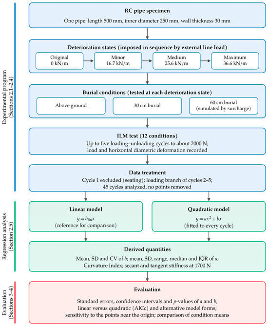
Figure 1 summarizes the research program. One RC pipe specimen was brought through four deterioration states in sequence; at each state it was tested with ILM under three burial conditions; and the loading branches of the retained cycles were analyzed with linear and quadratic regression models, from which the stiffness and curvature measures were derived and then evaluated statistically.
Figure 1.
Research program: experimental program, regression analysis and evaluation, with the corresponding sections.
2.1. Internal Loading Method and Device
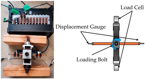
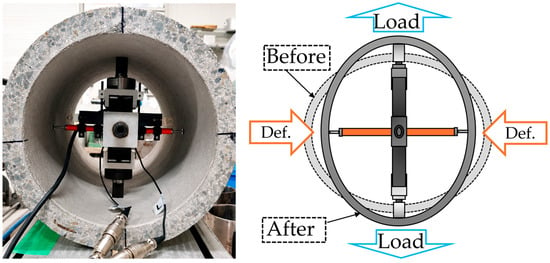
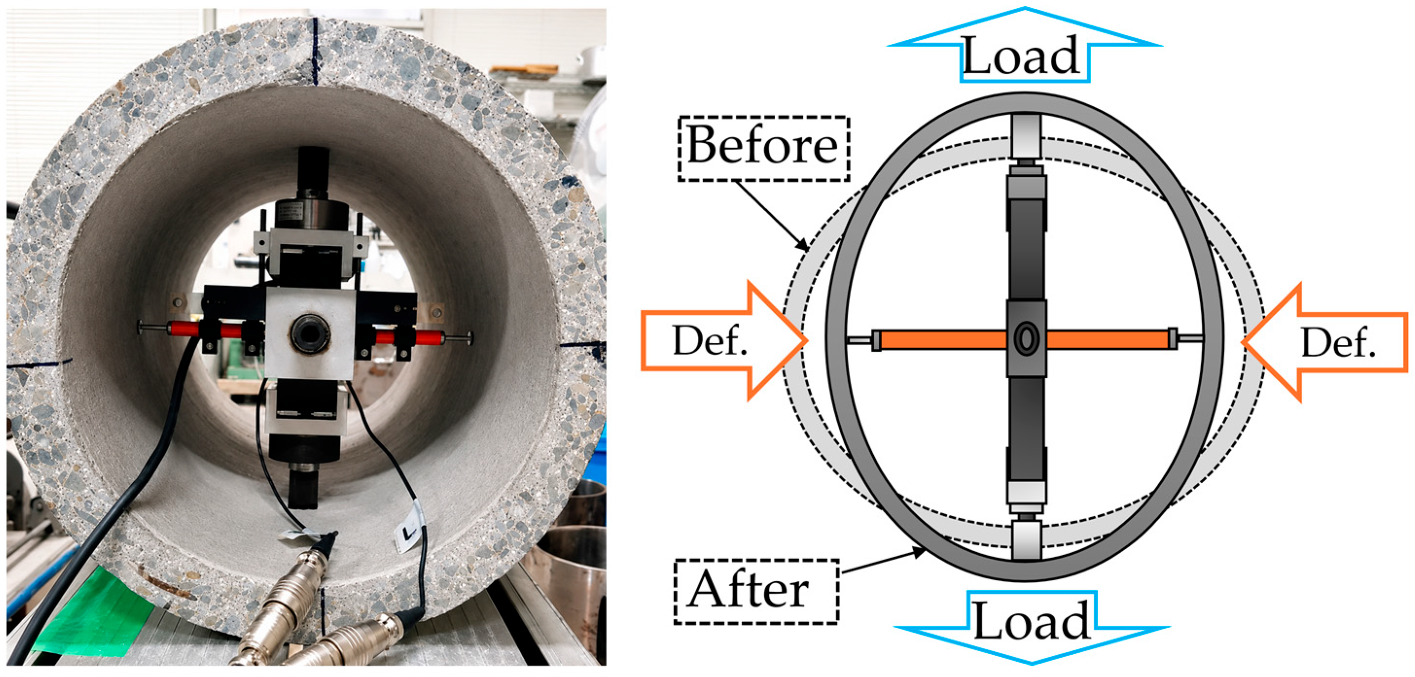
ILM is a non-destructive technique for the in situ structural evaluation of small- and medium-diameter buried pipes, typically those with internal diameters below 800 mm [39,41]. The ILD (Figure 2) is positioned at the cross-section of interest and applies a load through two diametrically opposed loading arms driven by a loading bolt; a calibrated load cell records the applied load. The loading arms push the crown and invert outward, so that the vertical diameter increases and the springlines move inward; the resulting deformation is measured by displacement gauges oriented perpendicular to the loading axis, that is, as the change in the horizontal diameter of the pipe (Figure 3). A reduction in the slope of the load–deformation response indicates a loss of cross-sectional stiffness.
Figure 2.
Manual Internal Loading Device (ILD): photograph (left) and schematic showing the load cells, loading bolt and displacement gauges (right).
Figure 3.
ILD positioned inside the RC pipe specimen (left) and measurement principle (right): outward loading at the crown and invert, and measurement of the horizontal diameter change.
Two ILD configurations exist: an automatic version intended for standardized field deployment and a manual version that permits finely controlled incremental loading with higher resolution and repeatability. The manual ILD was used throughout this study. Deformation readings were recorded in increments of 0.5 μm.
2.2. Pipe Specimen and Deterioration States
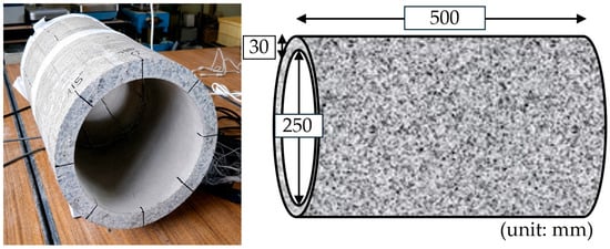
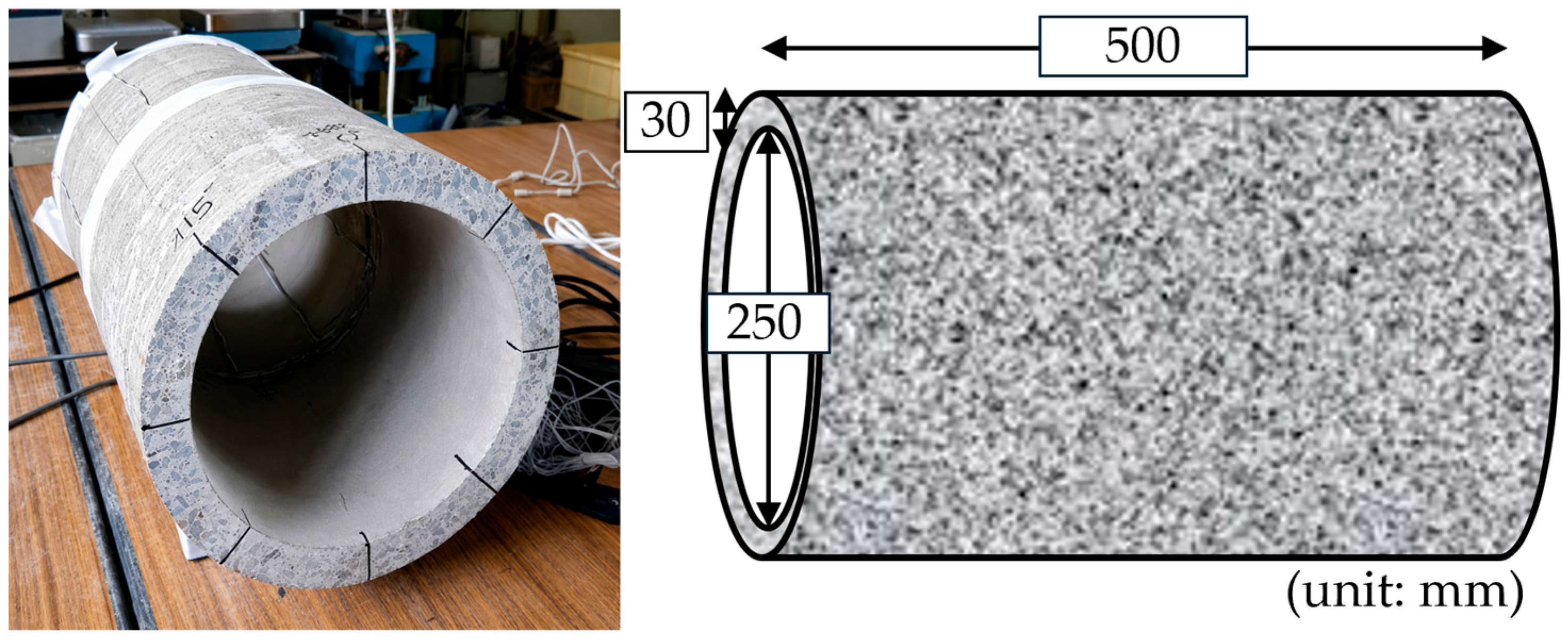
A single RC pipe, 500 mm long with an internal diameter of 250 mm and a wall thickness of 30 mm (outer diameter 310 mm; centerline diameter 280 mm), was tested (Figure 4 and Table 1). This size is representative of the small-diameter classes used in agricultural and urban buried networks. The specimen was dimensionally verified against the manufacturer’s specifications, and the inner wall was lightly sanded at the two loading points to ensure uniform load transfer. The elastic modulus in Table 1 was not measured on the present specimen; it was adopted from a previous study on an RC pipe supplied by the same manufacturer [40]. The ring stiffness was calculated per unit length as EI/D3, with I = t3/12 and D = Di + t = 280 mm, the centerline diameter.
Figure 4.
RC pipe specimen: photograph (left) and dimensions in mm (right).
Table 1.
Specifications of the tested pipe specimen.
Four deterioration states (original, minor, medium and maximum) were imposed sequentially on the same specimen by applying external line loads with a compression testing machine (Table 2). The load magnitudes correspond to the manufacturer-specified thresholds for this pipe class: crack initiation (minor), the load preceding significant fracturing (medium) and the maximum load before failure (maximum). Using one specimen removes inter-specimen variability in mix design, reinforcement placement and curing as a confounding factor, and mirrors the progressive accumulation of damage on a single asset; it also means that the results cannot be generalized beyond this specimen (Section 4.4). The deterioration states are defined by the applied load levels only: crack widths and crack patterns were not mapped, and no independent non-destructive measurement of the damage was made. After each deterioration load, ILM tests were conducted under all three burial conditions before the next load was applied.
Table 2.
External loads defining each deterioration state.
2.3. Burial Conditions
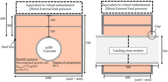
Three burial conditions were tested (Figure 5 and Table 3). In the above-ground condition, the pipe was tested without soil. For the 30 cm condition, the pipe was placed in a steel box (inner dimensions 1000 mm wide, 750 mm high and 400 mm long) and surrounded by decomposed granite soil compacted in layers to a degree of compaction of 90%, with 300 mm of soil above the crown. Because the pipe (500 mm) was longer than the box (400 mm), it passed through openings in the front and back walls and extended approximately 50 mm beyond each wall. A clearance was left around the pipe at these openings and sealed with tape to prevent loss of soil, so that the pipe did not touch the box and was supported only by the backfill. The loading cross-section was located at mid-length of the pipe, 200 mm from each wall. The 60 cm condition was simulated by placing steel weights on the soil surface of the 30 cm configuration to apply a surcharge equivalent to the weight of a further 300 mm of backfill. With a wet unit weight of 17.49 kN/m3 (dry density of 1.557 g/cm3 at 90% compaction and a water content of 14.5%), the nominal overburden pressure at the crown is approximately 5.25 kN/m2 for 300 mm of cover; the target surcharge was therefore approximately 5.25 kN/m2, giving a nominal overburden pressure of 10.5 kN/m2 for the simulated 60 cm condition (Table 3). These values are nominal overburden pressures; the earth pressure acting on the pipe was not measured. Design earth pressures of 15.8 and 30.5 kN/m2 were estimated with Marston’s trench formula [43,44], taking the full box width (1.0 m) as the trench width and dividing the resulting vertical load per unit length by the outer diameter of the pipe. The Marston formula is a general method for soil loads on buried pipes; under the present model conditions, however, using the full box width gives values about three times the weight of the soil directly above the crown, and it is uncertain whether the box can be treated as a conventional trench. In the present study, the test conditions are described by the nominal overburden pressure instead of these values. The pipe invert was approximately 140 mm above the steel floor of the box and the springlines were 345 mm from its side walls (Figure 5), so these rigid boundaries may have influenced the burial responses (Section 4.4).
Figure 5.
Steel model box used for the burial tests: front view (left) and side view (right); dimensions in mm.
Table 3.
Burial conditions and backfill properties.
2.4. Loading Cycles and Data Treatment
At each of the twelve conditions, up to five consecutive loading–unloading cycles were performed to approximately 2000 N, and the loading branch of each cycle was analyzed. The first cycle was excluded from all conditions to remove seating and contact-adjustment effects between the loading arms and the pipe wall [39], and the regression models (Section 2.5) were fitted independently to every remaining cycle (2nd to 5th). Two conditions yielded fewer than four post-seating cycles because of data-logging gaps, namely Original–60 cm (cycles 2–3) and Minor–Ground (cycles 2–4), giving 45 cycle-level fits in total. No cycle was excluded on the basis of its fitted coefficients, its agreement with an expected trend or its goodness-of-fit; exclusion was reserved for documented measurement abnormalities (sensor malfunction, signal discontinuity, missing data or loss of contact), and none was identified beyond the logging gaps noted above.
At the start of loading, several records contain small non-zero loads at zero deformation and occasional readings of −0.5 μm, which are attributed to contact seating and the 0.5 μm resolution of the deformation readings. These points were retained in all fits so that no data were selectively removed. In a fit forced through the origin, points at zero deformation do not affect the estimated coefficients, although they enter the residual sum of squares and hence the statistical evaluation; points with negative deformation, or points affected by the initial contact conditions, can affect a and b. Their influence was examined by refitting every cycle after removing the points with a load below provisional thresholds of 50, 100 and 200 N (Section 3.3 and Appendix A).
2.5. Regression Models and Derived Indices
Each loading cycle was described by a forced-origin second-degree polynomial:
where y is the applied load (N) and x is the measured diametric deformation (μm). The model passes through the origin, following established ILM practice [36,37,39]. This is an assumption, because several records show an apparent offset at the start of loading (Section 2.4); its influence on b is examined in Section 3.3. The linear coefficient b is referred to as the model-derived initial tangent stiffness: it is the slope of the fitted curve at x = 0, not a stiffness measured directly at zero deformation, because the readings near the start of loading are affected by contact seating and the 0.5 μm deformation resolution (Section 2.4); it is defined by the forced-origin quadratic model and is not a model-independent quantity. The quadratic coefficient a describes how the slope changes during loading; a < 0 indicates that the slope of the fitted load–deformation response decreases with increasing deformation (softening of the fitted response), which does not by itself demonstrate a reduction in the stiffness of the pipe material. Because a and b are estimated jointly from the same fit over a narrow deformation range, they are not statistically independent, and compensating covariation between them cannot be excluded; they are therefore interpreted as complementary rather than independent descriptors.
y = ax2 + bx
The second-order polynomial was retained for three reasons: it is the simplest extension of the linear ILM index that can represent a change in slope; it has only two parameters and is linear in them, so it can be fitted by ordinary least squares; and its linear coefficient b has a direct meaning as the initial tangent stiffness, comparable with the slope of the established linear index. To examine whether other functional forms describe the data equally well, four alternative two-parameter forms (power, exponential-saturation, hyperbolic and logarithmic) and a three-parameter bilinear form were fitted to every cycle under the same origin constraint and compared with the quadratic model (Section 3.2).
To show what the quadratic term adds, a forced-origin linear model was also fitted to the same data points over the same range:
y = blin x
The two models were compared graphically for one cycle of two conditions (Section 3.2) and statistically for all 45 cycles (Table A1). Both models were fitted by ordinary least squares, and goodness-of-fit was quantified with the coefficient of determination appropriate to a model without intercept, in which the total sum of squares is taken about zero:
where is the fitted load. Because the linear model is a special case of the quadratic model (a = 0), the quadratic R2 is never lower than the linear R2 for the same data; a small difference in R2 can therefore coexist with a systematic departure of the linear fit, which is examined through the residuals.
For each condition, b is summarized across cycles by its mean (), standard deviation (SD) and coefficient of variation (CV). The coefficient a is summarized by its mean (), SD, range and the proportion of cycles with a < 0; its CV is not reported because several conditions have means close to zero, for which the CV is numerically unstable; the median, the interquartile range (IQR) and the ratio SD/|median| of a are reported instead (Section 3.4 and Appendix A). Because the raw value of a depends on the deformation range over which it is fitted, a dimensionless Curvature Index (CI) was also computed for each cycle:
where xmax is the maximum deformation of the cycle. CI expresses the magnitude of the quadratic term relative to the linear term at the end of the tested range. Because it uses the absolute value of a, it represents the relative magnitude of the quadratic contribution, not the direction of curvature. Finally, because the slope of the quadratic response varies with deformation, two stiffness definitions were evaluated from the mean–cycle coefficients:
The secant stiffness ksec describes the total deformation under a given load and is the polynomial analog of the linear index k = F/δ, whereas the tangent stiffness ktan describes the incremental response at the current state. For cross-condition comparison, both were evaluated at a common reference load of 1700 N by solving ax2 + bx = 1700 for each condition. This is the highest round load reached within the tested deformation range, taken as the mean maximum deformation, by the mean–cycle curves of all twelve conditions (the limiting condition, Max–60 cm, reaches 1736.3 N), so that no extrapolation is required. Differences between the condition means of b were compared with the cycle-to-cycle scatter using Welch’s t-test on the cycle-level values. Because the cycles of one condition are repeated loadings of the same specimen and not independent specimens, the resulting p-values are used only as a descriptive guide.
For every cycle, the standard errors and 95% confidence intervals of a and b were obtained from the least-squares covariance matrix, and each coefficient was tested against zero with a t-test on n − 2 degrees of freedom, where n is the number of readings in the loading branch. Because the linear model is nested in the quadratic model, the F-test for the added term is equivalent to the t-test on a. The two models, and the alternative forms, were also compared with the small-sample Akaike information criterion (AICc) [45]; ΔAICc is defined as AICc(linear)−AICc(quadratic), so that positive values favor the quadratic model; ΔAICc > 2 is taken to favor the quadratic model, ΔAICc < −2 to favor the linear model, and |ΔAICc| ≤ 2 to indicate that the two are indistinguishable. For the seven functional forms, the form with the lowest AICc was also identified for each cycle; this is a different criterion from the pairwise ΔAICc classification. Collinearity between the x and x2 terms was quantified with the variance inflation factor (VIF) of the no-intercept model and with the correlation between the estimates of a and b. Successive readings within a loading cycle are not independent observations, and the cycles are repeated loadings of one specimen, so the resulting p-values are somewhat optimistic; the numbers of significant cycles and the ΔAICc classifications are therefore treated as exploratory evidence, not as formal tests. The same statistics, together with the adjusted R2 and the Bayesian information criterion (BIC), were computed for the linear model, and both models were also fitted to the pooled cycles of each condition. The pooled fits give a condition-level comparison but treat the cycles as interchangeable, so their p-values are even more optimistic.
The regression and statistical computations reported in Section 3.2, Section 3.3, Section 3.4, Section 3.5 and Section 3.6 and Appendix A were performed with Python (version 3.13) code generated and executed within Claude (Opus 5.5; Anthropic), which was also used to plot the results. The input data were the authors’ own measurements, and the authors verified the fitted coefficients of selected cycles against their own spreadsheet fits.
3. Results
3.1. Load–Deformation Responses of the Twelve Conditions
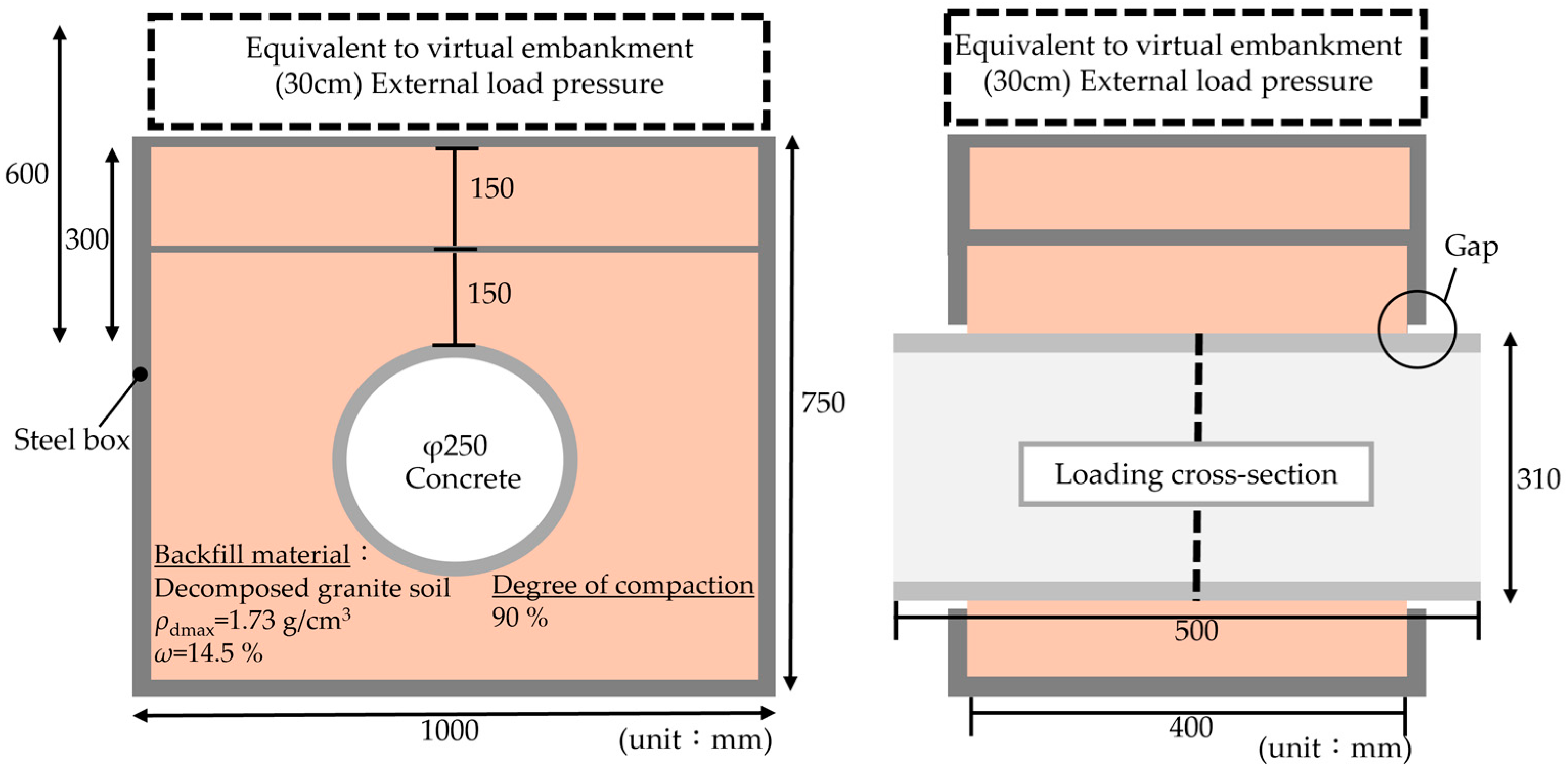
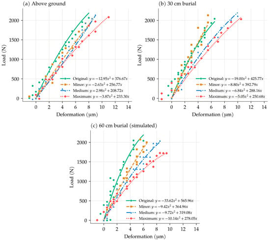
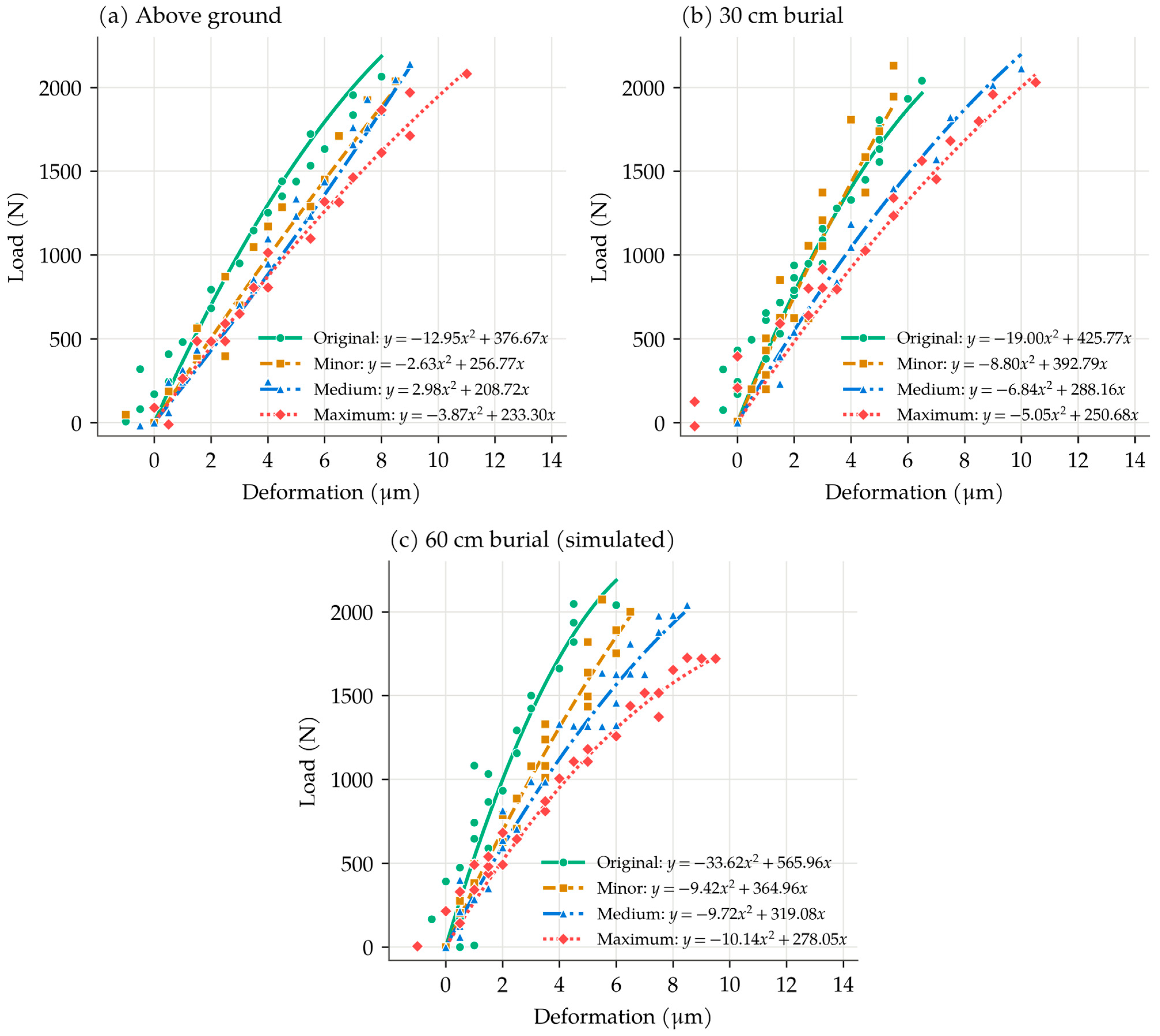
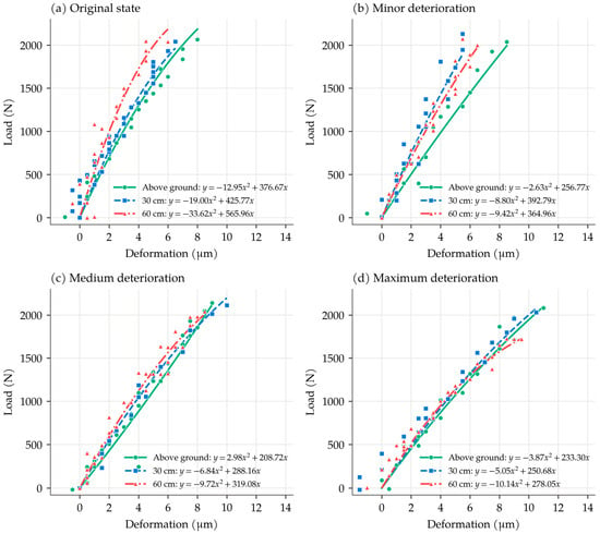
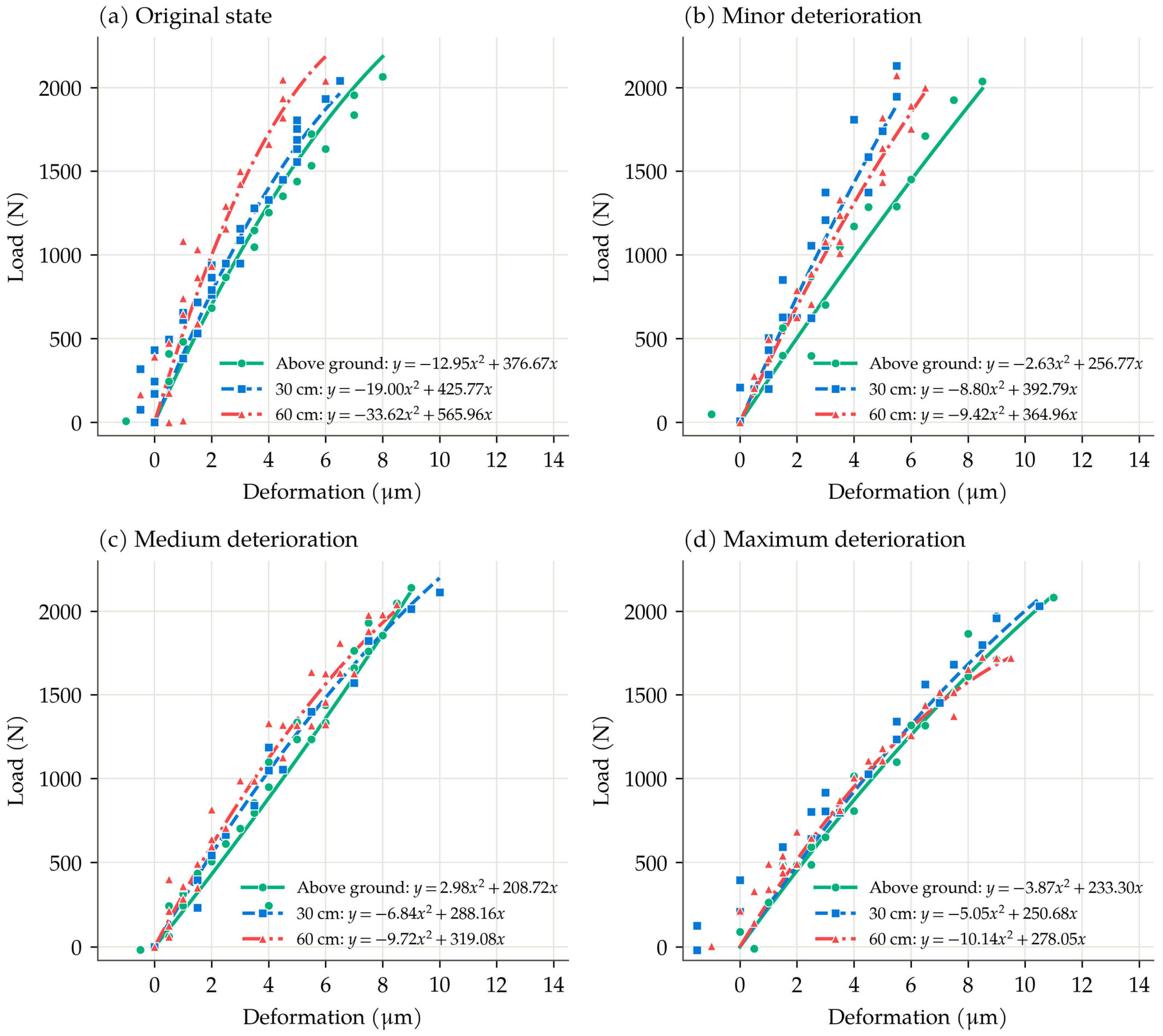
Figure 6 and Figure 7 show the load–deformation responses of all twelve conditions, grouped by burial condition and by deterioration state, respectively. The curves are plotted from the mean–cycle coefficients (Table 4), and the points show the measured data of one representative cycle per condition, the cycle whose a is closest to the condition mean among cycles 2–5; each curve is drawn over the deformation range of the plotted cycle. All responses are approximately proportional at the start of loading, and the deformation at about 2000 N increases from 5 to 7 μm for the original pipe to about 10 μm at maximum deterioration. Curvature is most visible for the original pipe, particularly at 60 cm burial, and least visible for the deteriorated states at ground level. The scatter of the points about the curves is largest at small deformations, where the load changes by several hundred newtons between successive 0.5 μm readings.
Figure 6.
Load–deformation responses of the four deterioration states under (a) above-ground, (b) 30 cm burial and (c) 60 cm burial conditions. Points: measured data of the representative cycle of each condition; curves: mean–cycle equations (Table 4).
Figure 7.
Load–deformation responses of the three burial conditions in the (a) original, (b) minor, (c) medium and (d) maximum deterioration states. Points: measured data of the representative cycle of each condition; curves: mean–cycle equations (Table 4).
Table 4.
Mean–cycle regression coefficients and reproducibility (cycles 2–5) by condition.
3.2. Linear Versus Quadratic Description
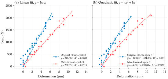
Figure 8 compares the linear and quadratic fits on identical data for two conditions: Original–30 cm, which shows clear curvature (, negative in all four cycles), and Max–Ground, in which curvature is less apparent (, also negative in all four cycles). For each condition, cycle 3 was used, and both models were fitted to the same measured points over the same range.
Figure 8.
Comparison of (a) linear and (b) quadratic fits to the same measured data for cycle 3 of Original–30 cm and cycle 3 of Max–Ground.
For Original–30 cm, the linear fit (blin = 341.38 N/μm, R2 = 0.9683) departs systematically from the measurements. It underestimates the load between approximately 1 and 3.5 μm, where the mean residual is +164 N at 1–2 μm and +60 N at 2.5–3.5 μm, and it overestimates the load from about 4 μm onward, increasingly toward the end of loading: the mean residual beyond 5.5 μm is −147 N and the residual at the last point (6.5 μm) is −179 N. The quadratic fit (a = −17.673, b = 424.36 N/μm, R2 = 0.9731) follows the decreasing slope and reduces the residual at the last point to +28 N. The difference is therefore not a uniform scatter but a curvature that a single slope cannot follow: the straight line is too shallow at the start of loading and too steep at the end.
For Max–Ground, the linear fit (blin = 207.83 N/μm, R2 = 0.9915) and the quadratic fit (a = −4.001, b = 239.00 N/μm, R2 = 0.9936) are close over most of the range: the linear fit slightly underestimates the load between 1 and 4.5 μm (mean residuals of +22 to +92 N), and the two fits nearly coincide between 5 and 9 μm. A departure appears only at the largest deformation (11 μm), where the linear fit overestimates the load by 204 N and the quadratic fit by 62 N. In both conditions the points at or near zero deformation lie above both fits; these reflect contact seating and reading resolution (Section 2.4) and are not described by either model. The comparison also shows why R2 alone is insufficient: the linear R2 exceeds 0.96 in both cases even where its departure is systematic.
The statistical support for the quadratic term was evaluated for every cycle (Table A1). In the two cycles of Figure 8, a differed significantly from zero (Original–30 cm: a = −17.67, 95% confidence interval −33.67 to −1.68, p = 0.032; Max–Ground: a = −4.00, 95% confidence interval −7.27 to −0.73, p = 0.019). Over the 45 cycles, b was significant in every fit (p < 0.001; relative standard error 3.7–20.0%), whereas a was significant at the 5% level in 28 cycles. The same 28 cycles had ΔAICc > 2, favoring the quadratic model, and the two models were indistinguishable in 12 cycles. In the remaining five (Minor–Ground cycle 3, Minor–30 cm cycles 4 and 5, Minor–60 cm cycle 3 and Max–30 cm cycle 4), ΔAICc was between −2.5 and −2.1. Because the linear model is nested in the quadratic model, the added term cannot increase the residual sum of squares, and a negative ΔAICc reflects only the penalty for the additional coefficient; with p = 0.50–0.98 for a, these values indicate that adding the quadratic term was not justified in these five cycles, rather than that the linear model was clearly superior. The adjusted R2 was higher for the quadratic model in 34 of the 45 cycles, and BIC, which penalizes the additional coefficient more strongly, favored the quadratic model by more than 2 in 25 cycles. The quadratic term was significant in every cycle of Original–30 cm, Medium–30 cm, Medium–60 cm and Max–60 cm, and in only one cycle of Minor–Ground, Minor–30 cm, Medium–Ground and Max–30 cm. As a supplementary condition-level check, which is not used as primary evidence because the pooled points come from repeated loadings of the same specimen, the cycles of each condition were also pooled: a was significant in all twelve conditions (negative in eleven; F-test p ≤ 0.017; ΔBIC > 2 in ten conditions; Table A2). The x and x2 terms are strongly collinear over the narrow tested range (VIF = 9.2–19.3; correlation between the estimates of a and b, −0.94 to −0.97), which explains the wide confidence intervals of a. Because of the inherent correlation between the first- and second-order terms, coefficient a was not interpreted as an independent quantitative deterioration index. The quadratic model therefore did not outperform the linear model in every cycle, although it gave a statistically meaningful improvement in a substantial number of cycles. Its value lies in describing load-dependent changes in apparent stiffness that a single linear coefficient cannot represent, not in being the best model under all conditions.
When the seven forms (Section 2.5) were compared by the lowest AICc in each cycle, a different criterion from the ΔAICc classification above, the quadratic model had the lowest AICc in 16 of the 45 cycles, the linear model in 10, the power form in 7, the hyperbolic and logarithmic forms in 5 each and the bilinear form in 2 (Table A3); the quadratic model was therefore not the best-fitting form in most cycles. The mean difference in AICc between each curved two-parameter form and the quadratic model was between −0.4 and +0.6. This small mean difference does not show that the forms are equivalent in each cycle, but it indicates that no single curved form was consistently superior on these data. All forms were fitted under the same origin constraint. The quadratic model is not claimed to be the optimal form; it is retained for its simplicity, its small number of parameters and the direct interpretation of b as the initial slope of the fitted curve; for some of the alternative forms, the slope at the origin is not finite.
3.3. Initial Tangent Stiffness
The cycle-level coefficients are summarized by condition in Table 4. The quadratic model described individual cycles well: across the 45 fits, R2 ranged from 0.922 to 0.998 (mean 0.983), and the mean R2 of every condition exceeded 0.96.
The mean model-derived initial tangent stiffness is used here to describe the effects of deterioration and burial. At 60 cm burial, decreased from 565.96 N/μm for the intact pipe to 364.96, 319.08 and 278.05 N/μm for the minor, medium and maximum states, an overall reduction of 50.9%; at this burial condition decreased at every step. At 30 cm, also decreased at every step but unevenly (by 7.7%, 26.6% and 13.0% for the successive transitions; 41.1% overall). At ground level, decreased from 376.67 to 256.77 and 208.72 N/μm between the original, minor and medium states but was higher (233.30 N/μm) at the maximum state. This difference of 24.58 N/μm is smaller than the cycle-to-cycle SD of Medium–Ground (46.07 N/μm) and is not statistically distinguishable (p = 0.37); the overall change from original to maximum was a reduction of 38.1%. The overall reductions from the original to the maximum state exceeded the cycle scatter under all three burial conditions (p = 0.004, 0.004 and 0.036 at ground level, 30 cm and 60 cm), whereas four of the nine changes between adjacent states did not (p > 0.05). With two to four cycles on one specimen, the stepwise changes are therefore reported descriptively, and only the overall reductions are interpreted. Deterioration therefore reduced overall under every burial condition, without a decrease at every step in every condition.
Burial increased in all four deterioration states when the above-ground and 60 cm conditions are compared (p = 0.011–0.031). The increase was smallest at maximum deterioration (233.30 to 250.68 to 278.05 N/μm; 19.2%) and between 42% and 53% in the other three states: 50.3% for the intact pipe (376.67 to 425.77 to 565.96 N/μm), 52.9% for the medium state (208.72 to 288.16 to 319.08 N/μm) and 42.1% for the minor state, which increased by 53.0% from ground level to 30 cm and then decreased by 7.1% from 30 cm to 60 cm; this decrease is within the cycle scatter (p = 0.48). In this specimen, the burial gain was therefore smallest at the maximum deterioration state, but the gain did not diminish steadily with deterioration, and the three less deteriorated states cannot be ranked; whether this is a general trend requires further specimens.
Reproducibility of b differed between conditions: CVb ranged from 1.6% (Medium–30 cm) to 22.1% (Medium–Ground). Medium–Ground, which also shows a lower ground-level mean than the maximum state and an anomalous sign of a (Section 3.4), is the least reproducible condition and is treated as an exception rather than folded into the trend. In eleven of the twelve conditions, exceeded the forced-origin linear slope fitted to the same cycles (Section 3.2), as expected for a tangent evaluated at x = 0 before softening reduces the local slope; the exception is Medium–Ground, whose mean a is positive, so that its linear slope exceeds .
Because b is the slope at the origin of a curve forced through the origin, it can be affected by the readings near the start of loading (Section 2.4). All 45 cycles were therefore refitted after removing the points with a load below provisional thresholds of 50, 100 and 200 N (Table A4). These thresholds were used to examine the sensitivity of the results to the initial readings, not to identify the end of seating; the load corresponding to one reading step of 0.5 μm, estimated as b × 0.5 μm, is approximately 100–280 N, but this does not indicate the load at which seating is completed either. With the 50 N threshold, of Original–60 cm increased from 565.96 to 584.15 N/μm (+3.2%), and changed by at most 6.7% in any condition (Original–Ground). Across the three thresholds, the overall reduction of at 60 cm was 50.9–52.7%, and the burial gain from ground level to 60 cm was 44.4–48.4% for the original state and 20.4–21.9% for the maximum state; the largest gain remained in the medium state and the smallest in the maximum state, and Medium–Ground remained the only condition in which the linear slope exceeded . The order of the reductions at ground level and at 30 cm was reversed (41.4% and 37.6% at 50 N), so these two values are not ranked.
The same refits were used to examine a. With all points and with the three thresholds, a was negative in 40–41 cycles and significant in 28–31 cycles, and the ΔAICc classification changed little (Table A4). The sign changes in Minor–60 cm and Medium–Ground persisted at every threshold, whereas the single positive cycle of Minor–Ground became negative at 200 N. The magnitudes of a and b, however, changed together: increased by up to 14.3% and became more negative by up to 83% (Max–30 cm at 200 N), consistent with the strong correlation between the two estimates, and removing readings also reduced the number of points per cycle. The seating points therefore did not alter the main trends of or the sign and significance of a, whereas the magnitude of a was sensitive to them.
3.4. Curvature Coefficient
A negative value of a indicates a decreasing slope in the fitted load–deformation response. This tendency was observed in 40 of the 45 cycles (88.9%) and was statistically significant in 27 cycles; one further cycle (Medium–Ground, cycle 4) had a significantly positive a (Table A1). A negative but non-significant value does not provide sufficient statistical evidence of curvature, and even a significantly negative a describes the fitted response; it does not by itself demonstrate a reduction in the stiffness of the pipe material. Its sign was consistent in nine conditions, in which every cycle gave a < 0: all three original conditions, Minor–30 cm, Medium–30 cm, Medium–60 cm and all three maximum-deterioration conditions (Table 4). In the remaining three conditions, the sign changed between cycles: Minor–Ground (2 of 3 cycles negative; range −4.231 to +0.080), Minor–60 cm (3 of 4; −17.202 to +2.920) and Medium–Ground (1 of 4; −2.396 to +8.199, with a positive mean of +2.978). The causes of these sign changes cannot be identified with the present data; reading resolution and contact conditions are possible contributors.
The magnitude of did not follow a consistent trend with deterioration, and the values below are reported descriptively rather than as a ranking of deterioration. At 30 cm, decreased across the four states (19.003, 8.799, 6.836 and 5.050); at 60 cm it dropped from 33.622 to 9.421 between the original and minor states and then remained approximately constant (9.717 and 10.142); at ground level it changed sign between the minor, medium and maximum states. The variability of a between cycles was large: its SD ranged from 1.041 to 9.169 N/μm2 and its IQR from 0.879 to 7.094 N/μm2 (Table 4 and Table A5). Relative variability is expressed with respect to the median: SD/|median| ranged from 0.15 (Medium–30 cm) to 1.43 (Minor–30 cm) and exceeded 0.4 in nine of the twelve conditions (Table A5). The median is used because the mean of a is close to zero in some conditions, which makes a ratio to the mean unstable (for example, 1.46 for Medium–Ground). In addition, xmax differed between conditions, so raw values of a fitted over different ranges are not directly comparable. A high R2 confirms that the quadratic curve follows each cycle, but it does not establish that the cycle-to-cycle variation in a is mechanical: reading resolution, loading-arm contact, the narrow fitting range and the covariance between a and b may all contribute, and their contributions cannot be separated with the present data. The quadratic equation therefore describes the curvature of each loading response, but the present results do not justify using a as a quantitative measure of deterioration severity: a significantly negative a indicates a decreasing slope of the fitted response, whereas the magnitude of a, which was also sensitive to the treatment of the initial readings (Section 3.3), should not presently be interpreted as a deterioration index.
3.5. Curvature Index
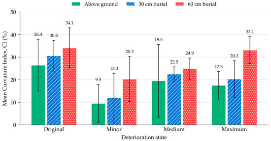
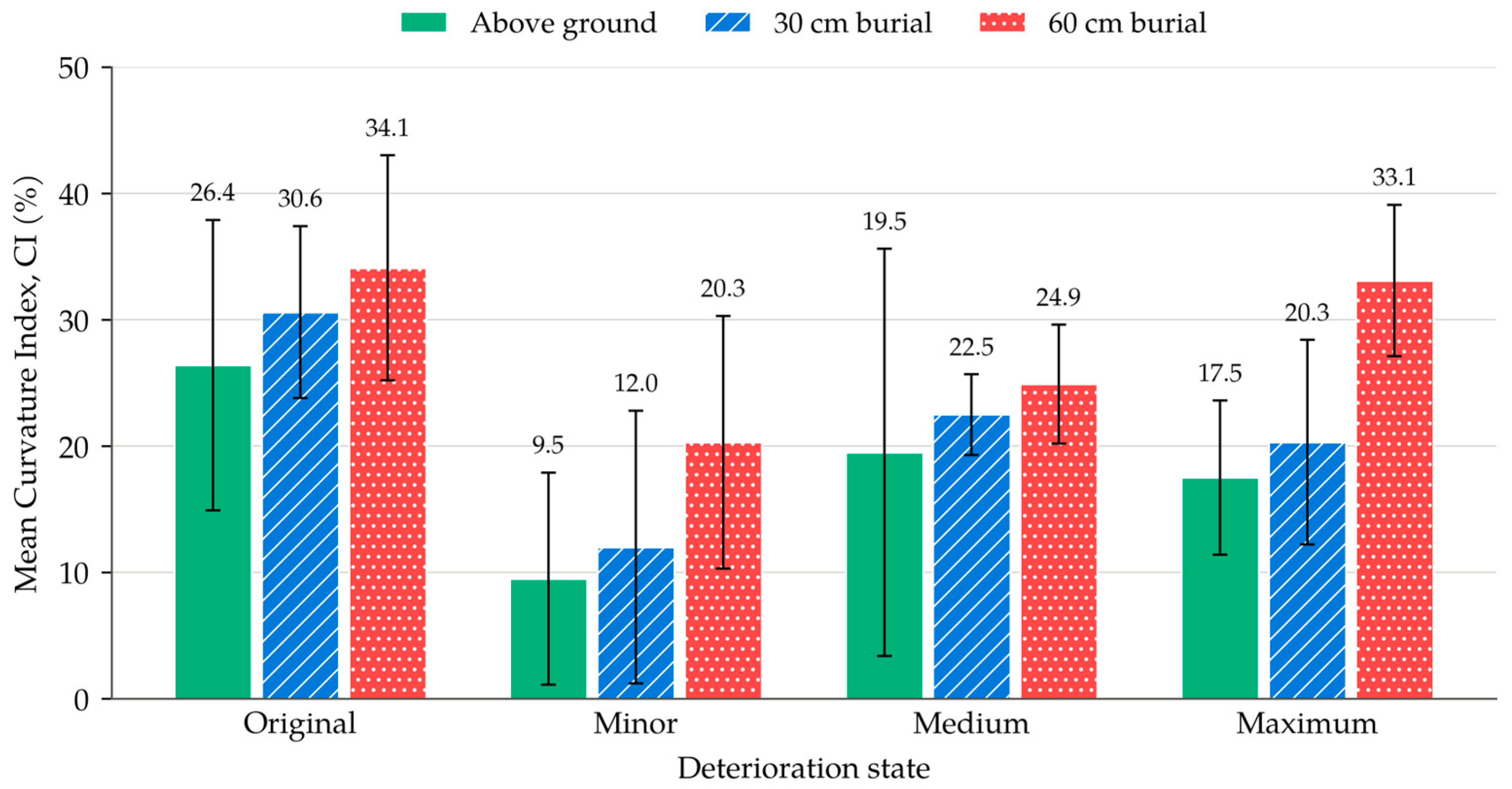
The mean CI increased with burial depth, from 18.2% at ground level to 21.3% at 30 cm and 28.1% at 60 cm (Table 5 and Figure 9), indicating that, across the dataset, the curvature was more pronounced relative to the linear term under greater confinement. Because CI uses the absolute value of a, cycles with a positive a (for example, three of the four cycles of Medium–Ground) also contribute to the mean CI; CI therefore represents the relative magnitude of the quadratic contribution, not the direction of curvature, and it inherits the variability of a: the relative SD reached 90.3% (Minor–30 cm), 88.4% (Minor–Ground) and 82.3% (Medium–Ground), whereas conditions with a consistent a, such as Medium–30 cm (14.3%) and Max–60 cm (18.1%), gave reproducible values. CI is therefore used only as a dataset-level indicator of the practical significance of curvature, not as a condition-specific diagnostic. As Figure 9 shows, the error bars (±1 SD) of the three burial conditions overlap in the original, minor and medium states; only at maximum deterioration do the ground-level and 60 cm values separate. The increase in the mean CI with burial depth is therefore a tendency of the dataset, not a difference established for each state.
Table 5.
Mean Curvature Index (CI) by condition, with cycle-level reproducibility.
Figure 9.
Mean Curvature Index (CI) by deterioration state and burial condition; error bars show ±1 SD across cycles (values in Table 5).
3.6. Secant and Tangent Stiffness
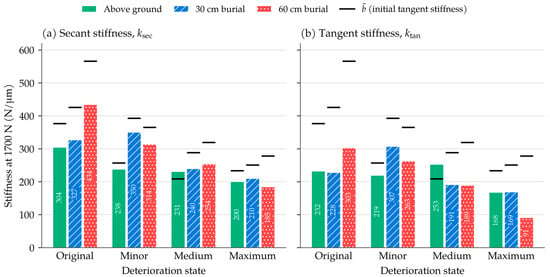
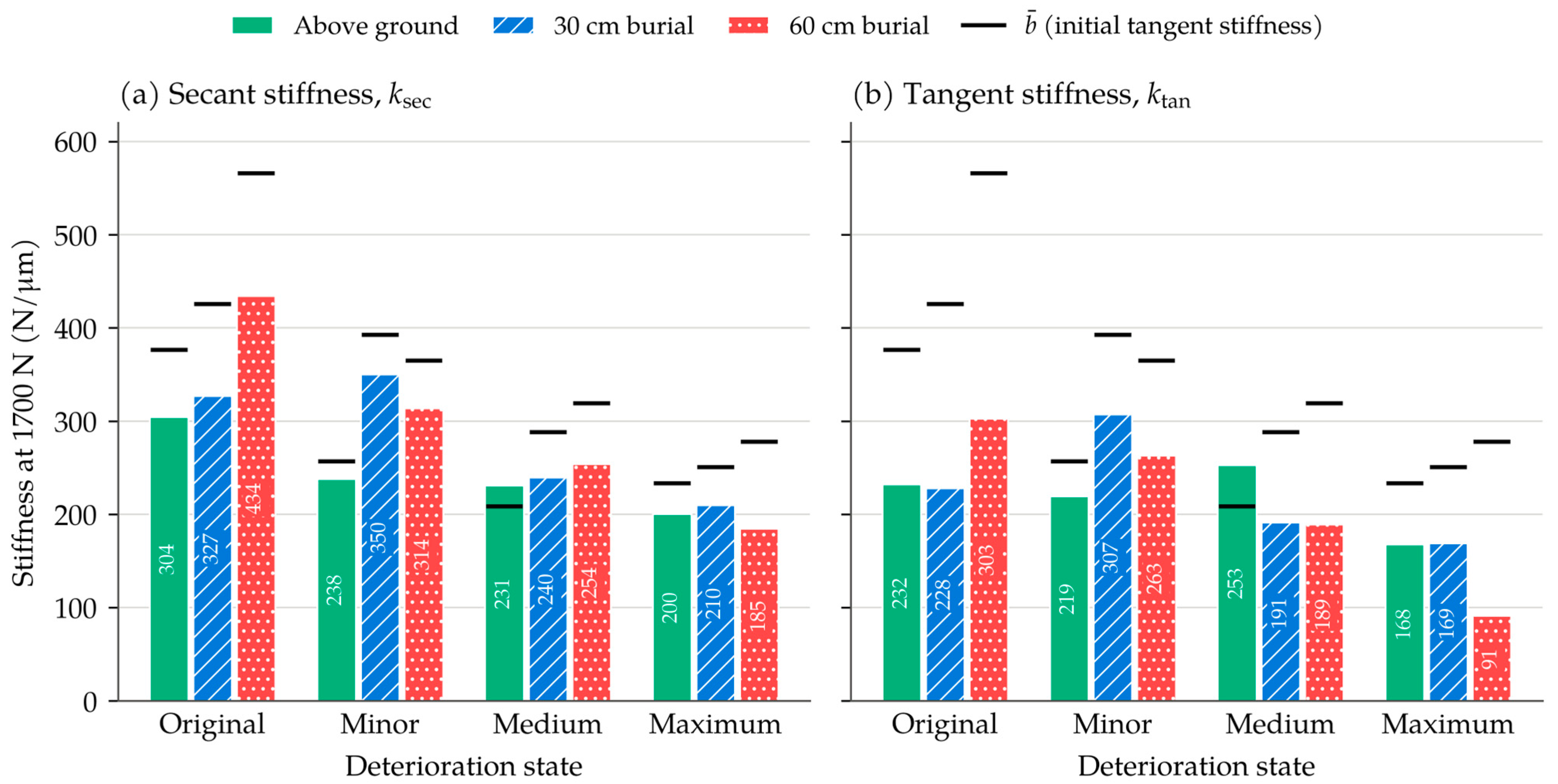
Under the quadratic model, the slope of the response varies with deformation. For Original–60 cm (y = −33.622x2 + 565.96x), the tangent stiffness decreased from 565.96 N/μm at x = 0 to 364.23 N/μm at x = 3 μm and to 179.31 N/μm at the mean tested limit (x = 5.75 μm), a reduction of 68.3% within the tested range. Table 6 and Figure 10 give both stiffness definitions at the 1700 N reference load (Section 2.5). The required deformation lay within the mean tested range in all twelve conditions, at 68–96% of the mean maximum deformation. The reference load is lower than the approximately 2000 N reached by the individual cycles because the Max–60 cm mean–cycle curve reaches only 1736.3 N at its mean tested limit (x = 9.62 μm), and its vertex (1905.7 N) also lies outside the tested domain. This is attributed to averaging cycles of different curvature, not to a physical loss of stiffness near 1900 N.
Table 6.
Secant and tangent stiffness at the 1700 N reference load, from the mean–cycle coefficients.
Figure 10.
(a) Secant and (b) tangent stiffness at the 1700 N reference load by deterioration state and burial condition; the horizontal marks show (values in Table 6).
At the reference load, the secant stiffness was 66–93% of and the tangent stiffness 33–85% of in the eleven conditions with ; Medium–Ground, with a positive , is the exception. At 60 cm burial, ksec decreased with deterioration (434.4, 313.9, 254.1 and 184.7 N/μm), following the same order as . Because is defined at x = 0 for every condition, it is retained as the primary comparison parameter in this study, with ksec at 1700 N as a secondary, practically interpretable value. Figure 10 shows the same information graphically: the secant stiffness lies furthest below for Max–60 cm (66%) and for the original pipe (77–81%), and closest for the minor state at ground level and 30 cm (89–93%).
4. Discussion
4.1. Roles of the Two Quadratic Coefficients
The results assign different roles to the two coefficients. The model-derived initial tangent stiffness reflects the effects of deterioration and burial: it decreased from the original to the maximum state under all three burial conditions, although not at every step, and was higher at 60 cm than at ground level in all four deterioration states of this specimen, with the smallest burial gain at maximum deterioration. The comparison in Figure 8 shows why a quadratic description is useful: where curvature is clear, a single slope underestimates the load at the start of loading and overestimates it near the end, so that a linear index averages two different parts of the response. The curvature coefficient a describes this change in slope within a cycle. A negative a, indicating a decreasing slope of the fitted response, was found in 40 of the 45 cycles and in every cycle of nine conditions, but it was significantly negative in only 27 cycles (the quadratic term was significant in 28 cycles in total, one of them with a positive a), and its magnitude varied widely between cycles and did not follow the order of deterioration. The quadratic equation should therefore be read as a description of the shape of the loading response, with as the most consistent of the descriptors examined in this dataset and a as a qualitative descriptor of the change in slope: a significantly negative a indicates a decreasing slope of the fitted response, which does not by itself demonstrate a loss of material stiffness, whereas the magnitude of a should not presently be interpreted as a deterioration index. The quadratic representation is therefore not presented as superior to the linear model in every cycle; its contribution is to capture load-dependent changes in apparent stiffness that cannot be represented by a single linear coefficient.
The following mechanical interpretation is inferred from the observations; the mechanisms were not measured directly. Physically, the diametric deformation of an elastic ring under a pair of opposed radial loads is proportional to the load and inversely proportional to the flexural rigidity of the wall, so b is an apparent stiffness of the loaded cross-section. It reflects the rigidity of the pipe wall and, for a buried pipe, the additional restraint of the surrounding soil, together with the local contact conditions at the loading arms. Cracking reduces the effective flexural rigidity of the wall, which is consistent with the overall decrease of with deterioration. During ILM loading, the loading arms push the crown and invert outward, and the springlines move inward (Section 2.1). The surrounding soil may restrain the outward movement of the crown and invert during vertical internal loading, thereby reducing the associated inward movement of the springlines. This mechanism is consistent with the observed increase in apparent stiffness under burial, although the contributions of soil confinement and boundary conditions were not quantified separately. In the sense of a scalar damage variable, the ratio of to its value in the original state is a residual-stiffness ratio; at the maximum state it was 0.62, 0.59 and 0.49 at ground level, 30 cm and 60 cm, respectively. This ratio is the only quantitative measure of damage available in this study and is specific to this specimen. A negative a means that the tangent slope of the fitted response decreases as the load increases. At the small loads applied here, this may arise from the opening of existing cracks, from nonlinear contact at the loading points or, under burial, from the stress-dependent response of the backfill; the present measurements cannot separate these sources, and no damage-mechanics parameter is therefore assigned to a.
These results can be related to previous work. Earlier ILM studies described the response with a single slope [36,37,38,39,40,42], and a strong positive correlation between load and deformation was reported for a buried RC pipe with and without earth pressure [40]. The present data agree with this: the forced-origin linear model gave R2 ≥ 0.919 in every cycle. The quadratic analysis adds that the departure from the straight line is systematic where curvature is clear, and that a single slope then lies below the initial tangent stiffness. In three-edge bearing tests, RC pipes show an approximately linear load–deflection response up to cracking, followed by a progressive loss of stiffness as cracks develop [4,23]. The ILM load of about 2 kN is about one quarter of the external line load that initiated cracking in this 0.5 m long specimen (16.7 kN/m), although the two loading arrangements are not equivalent; the softening within an ILM cycle is therefore not attributed to new cracking, which is consistent with the non-destructive character of the method. The increase of under burial is also in line with experimental and numerical studies in which the burial depth and the support of the surrounding soil were found to govern the deformation of buried pipes [6,31,32,33]. Those studies concern external loading; the present results show that an internal diagnostic load is affected by the burial condition in the same direction, which is why the burial condition has to be recorded with every ILM measurement.
4.2. Exceptions
Four exceptions qualify the general trends and are reported rather than smoothed. First, Medium–Ground is the least reproducible condition (CVb = 22.1%), its is positive, and at ground level was lower at the medium than at the maximum state, although this difference is within the cycle scatter (Section 3.3). Second, the minor state shows sign changes of a at ground level and at 60 cm, and its decreased from 30 cm to 60 cm, also within the cycle scatter. Third, Original–60 cm, which shows the strongest curvature, is based on two cycles only and has the lowest mean R2 (0.961); the lowest single-cycle value (0.922) occurred in Original–Ground. Fourth, the mean–cycle curve of Max–60 cm reaches only 1736.3 N within its tested range, which limited the common reference load to 1700 N (Section 2.5). Several of these exceptions coincide, which points to measurement variability in particular conditions rather than to distinct mechanical behavior, although the present data cannot separate the two.
4.3. Implications for ILM-Based Assessment
For ILM practice, the present results suggest that reporting the quadratic fit alongside the linear index may be useful, particularly under deeper burial, where curvature and the difference between secant and tangent stiffness are largest. In this specimen, the burial-related gain in ILM stiffness was smallest for the most deteriorated state (19.2%) and between 42% and 53% for the other three states; burial correction should therefore be examined on further specimens before a general correction factor is proposed. Such condition-resolved experimental data, including their variability and exceptions, can provide validation data for future numerical and model-based assessment of buried pipes.
4.4. Limitations
Several limitations qualify these findings. First, all measurements were made on one specimen, so between-specimen variability and the generality of the non-monotonic trends cannot be assessed; it cannot be determined whether the non-monotonic changes and the large scatter of some conditions (for example, a CV of 22.1% for Medium–Ground) reflect measurement variability or mechanical behavior, and the results should be regarded as preliminary until they are reproduced on several specimens. Second, a and b are estimated jointly and are strongly correlated (Section 3.2), so that a is identified only with wide confidence intervals and is not significant in 17 of the 45 cycles; moreover, successive readings are not independent and the cycles are repeated loadings of one specimen, so the statistical results are exploratory evidence. Third, the 60 cm condition was simulated by a surcharge on a 30 cm burial rather than by physical cover; the earth pressure on the pipe was not measured, and the steel floor (about 140 mm below the invert) and the side walls (345 mm from the springlines) of the model box are close enough to the pipe to have influenced the burial responses. The burial results therefore describe this laboratory configuration and should not be transferred directly to field burial depths. A surcharge reproduces the additional vertical stress of a deeper cover but not its geometry (arching, load spreading and lateral stress); a comparison with a physical 60 cm burial was not possible in the 750 mm high box and is left for future work. Fourth, deformation was read at a resolution of 0.5 μm, which is a substantial fraction of the deformations at the start of loading. Fifth, the model is forced through the origin, whereas several cycles begin with deformation readings at or below zero under loads of up to several hundred newtons. The thresholds used to examine this (Section 3.3) are provisional and do not remove the influence of seating completely, and a quadratic with a free intercept gave condition-mean intercepts of up to about 295 N. The forced-origin constraint may therefore affect the estimated coefficients and the percentages derived from them, although the overall decrease of b with deterioration, the comparatively small burial effect at maximum deterioration and the sign and significance of a were obtained under all four treatments. Sixth, the deterioration states are defined by load levels only, without crack mapping or an independent non-destructive measurement, and the 500 mm specimen is of the same order as the longitudinal extent over which a local internal load is transmitted in a buried RC pipe [40], so end effects cannot be excluded. Multi-specimen tests with finer deformation resolution are needed before the curvature coefficient can be evaluated as a condition-specific indicator.
5. Conclusions
The load–deformation responses of an RC pipe tested with the Internal Loading Method under four deterioration states and three burial conditions were described with a forced-origin quadratic model fitted to 45 loading cycles. This preliminary study examined the feasibility of the quadratic representation on a single specimen.
Scientific findings:
- On identical data, a linear fit departed systematically from the measurements where curvature was clear, underestimating the load at small-to-intermediate deformation and overestimating it near the end of loading; the quadratic model followed this change in slope. Where curvature was weak, the two fits were close except at the largest deformation.
- The mean model-derived initial tangent stiffness decreased overall with deterioration under all burial conditions, by 50.9% at 60 cm, 41.1% at 30 cm and 38.1% at ground level. These overall reductions exceeded the cycle-to-cycle scatter, whereas several changes between adjacent states, including the apparent increase from the medium to the maximum state at ground level, did not.
- Burial increased from ground level to 60 cm in all deterioration states of this specimen, least at maximum deterioration (19.2%) and by 42–53% in the other three states; the gain did not diminish steadily with deterioration, and whether the smaller gain at the maximum state is a general trend requires further specimens.
- A negative curvature coefficient a, indicating a decreasing slope of the fitted load–deformation response, was found in 40 of the 45 cycles and in every cycle of nine of the twelve conditions, but it was significantly negative in only 27 cycles, and one further cycle had a significantly positive a (28 significant cycles in total); a negative but non-significant value does not provide sufficient evidence of curvature. The sign of a changed between cycles in Minor–Ground, Minor–60 cm and Medium–Ground, and its magnitude did not follow the order of deterioration and was sensitive to the treatment of the initial readings.
Practical implications for ILM-based assessment:
- 5.
- The mean model-derived initial tangent stiffness was the most consistent of the descriptors examined in this dataset and is suggested, as a preliminary result, as the comparison parameter of an ILM record. Under burial, where the response is curved, a single linear slope lies below the initial stiffness, so reporting the quadratic fit alongside the linear index may be useful.
- 6.
- Burial changed by 19–53%, which is of the same order as the change caused by deterioration (38–51%). A stiffness measured by ILM on a buried pipe should therefore be interpreted against a reference obtained under the same burial condition, and burial correction should be examined on further specimens before a general correction factor is proposed.
- 7.
- The magnitude of a should not be used as a deterioration index. The present results are preliminary: they were obtained from a single specimen, with a deformation resolution of 0.5 μm and a model forced through the origin, and multi-specimen tests with finer resolution are required before threshold values can be proposed for practice.
Author Contributions
Conceptualization, M.H.; methodology, M.E. and M.H.; validation, M.H. and H.O.; formal analysis, M.E.; investigation, M.E. and M.H.; resources, M.H.; data curation, M.E.; writing—original draft preparation, M.E.; writing—review and editing, M.H. and H.O.; visualization, M.E.; supervision, M.H. and H.O.; funding acquisition, M.H. All authors have read and agreed to the published version of the manuscript.
Funding
This research was funded by the Japan Society for the Promotion of Science (JSPS) KAKENHI, grant number 26K09015.
Data Availability Statement
The data supporting the findings of this study are available from the corresponding author upon reasonable request, subject to approval by the supervising institution.
Acknowledgments
The authors thank the staff of the United Graduate School of Agricultural Sciences, Tottori University, for their support during the experimental program. This article is a revised and expanded version of a short communication entitled “Non-Destructive Assessment of Buried RC Pipes: A Polynomial Internal Loading Method Analysis of Stiffness and Softening Across Deterioration and Burial Conditions”, which was presented at OMNI 2026, the 1st International Seminar on Optimal Management and Non-destructive Testing for Civil and Industrial Infrastructure, İzmir, Türkiye, 29–30 September 2026 [46]. Preliminary results were also presented at Cairo Water Week 2026 (Egypt). During the preparation of this manuscript, the authors used Claude (Opus 5.5; Anthropic) for the data analysis and the plotting of graphs, as described in Section 2.5, and for assistance in drafting and editing the text based on drafts prepared by the authors. The authors have reviewed and edited the output and take full responsibility for the content of this publication.
Conflicts of Interest
The authors declare no conflicts of interest.
Abbreviations
The following abbreviations are used in this manuscript:
| AICc | Small-sample Akaike information criterion |
| BIC | Bayesian information criterion |
| CI | Curvature Index |
| CV | Coefficient of variation |
| ILD | Internal Loading Device |
| ILM | Internal Loading Method |
| IQR | Interquartile range |
| RC | Reinforced concrete |
| SD | Standard deviation |
| SE | Standard error |
| VIF | Variance inflation factor |
Appendix A
Table A1 lists the cycle-level statistics of the quadratic fits (Section 2.5 and Section 3.2), and Table A2 those of the linear and quadratic models fitted to the pooled cycles of each condition (Section 3.2). Table A3 compares the seven functional forms fitted to each cycle (Section 3.2), Table A4 reports the sensitivity of the mean coefficients to the readings recorded near the start of loading (Section 2.4 and Section 3.3), and Table A5 gives alternative measures of the variability of the curvature coefficient (Section 3.4).
Table A1.
Cycle-level statistics of the forced-origin quadratic fits (45 cycles): coefficients with standard errors (SEs), 95% confidence interval and p-value of a, coefficients of determination of the linear and quadratic models, and ΔAICc = AICc(linear)−AICc(quadratic).
Table A2.
Statistics of the linear and quadratic models fitted to the pooled cycles of each condition: coefficients with standard errors (SEs), p-value of a, linear coefficient blin (N/μm), adjusted R2, F-statistic of the nested comparison and ΔAICc and ΔBIC (positive values favor the quadratic model).
Table A3.
Comparison of seven functional forms fitted to each loading cycle (all forced through the origin): number of cycles in which each form had the lowest AICc, by condition (cycles 2–5).
Table A4.
Sensitivity of the mean coefficients to the initial readings: (N/μm) and (N/μm2) fitted with all points and after removing the points with a load below 50, 100 and 200 N (cycles 2–5).
Table A5.
Median, interquartile range (IQR) and SD/|median| of the curvature coefficient a by condition (cycles 2–5).
References
- Chaudhari, B.; Panda, B.; Šavija, B.; Paul, S.C. Microbiologically induced concrete corrosion: A concise review of assessment methods, effects, and corrosion-resistant coating materials. Materials 2022, 15, 4279. [Google Scholar] [CrossRef] [Scilit] [PubMed]
- Salihu, C.; Hussein, M.; Mohandes, S.R.; Zayed, T. Towards a comprehensive review of the deterioration factors and modeling for sewer pipelines: A hybrid of bibliometric, scientometric, and meta-analysis approach. J. Clean. Prod. 2022, 351, 131460. [Google Scholar] [CrossRef] [Scilit]
- Otegui, J.L. Challenges to the integrity of old pipelines buried in stable ground. Eng. Fail. Anal. 2014, 42, 311–323. [Google Scholar] [CrossRef] [Scilit]
- Wang, Y.; Li, P.; Liu, H.; Wang, W.; Guo, Y.; Wang, L. The effect of microbiologically induced concrete corrosion in sewer on the bearing capacity of reinforced concrete pipes: Full-scale experimental investigation. Buildings 2022, 12, 1996. [Google Scholar] [CrossRef] [Scilit]
- Zhu, Z.; Zhang, P.; Ma, B.; Zeng, C.; Zhao, Y.; Wang, F.; Li, Z.; Xiang, W.; Ariaratnam, S.T.; Yan, X. Quantitative model for residual bearing capacity of corroded reinforced concrete pipe based on failure mode. Tunn. Undergr. Space Technol. 2022, 129, 104675. [Google Scholar] [CrossRef] [Scilit]
- Shmulevich, I.; Galili, N. Deflections and bending moments in buried pipes. J. Transp. Eng. 1986, 112, 345–357. [Google Scholar] [CrossRef] [Scilit]
- Shcherban’, E.M.; Stel’makh, S.A.; Mailyan, L.R.; Beskopylny, A.N.; Smolyanichenko, A.S.; Chernil’nik, A.; Elshaeva, D.; Beskopylny, N. Analytical review of the current state of technology, structure formation, and properties of variatropic centrifugally compacted concrete. Materials 2024, 17, 1889. [Google Scholar] [CrossRef] [Scilit] [PubMed]
- Buried Timebombs: Saitama Sinkhole Draws Attention to Japan’s Aging Wastewater Infrastructure. Nippon.com. 2025. Available online: https://www.nippon.com/en/in-depth/d01102/ (accessed on 23 September 2026).
- Hao, T.; Rogers, C.D.F.; Metje, N.; Chapman, D.N.; Muggleton, J.M.; Foo, K.Y.; Wang, P.; Pennock, S.R.; Atkins, P.R.; Swingler, S.G.; et al. Condition assessment of the buried utility service infrastructure. Tunn. Undergr. Space Technol. 2012, 28, 331–344. [Google Scholar] [CrossRef] [Scilit]
- Yang, M.D.; Su, T.C. Segmenting ideal morphologies of sewer pipe defects on CCTV images for automated diagnosis. Expert Syst. Appl. 2009, 36, 3562–3573. [Google Scholar] [CrossRef] [Scilit]
- McKim, R.A.; Sinha, S.K. Condition assessment of underground sewer pipes using a modified digital image processing paradigm. Tunn. Undergr. Space Technol. 1999, 14, 29–37. [Google Scholar] [CrossRef] [Scilit]
- Cheng, J.C.P.; Wang, M. Automated detection of sewer pipe defects in closed-circuit television images using deep learning techniques. Autom. Constr. 2018, 95, 155–171. [Google Scholar] [CrossRef] [Scilit]
- Lai, Q.; Xin, Q.; Tian, Y.; Chen, X.; Li, Y.; Wu, R. Structural analysis and 3D reconstruction of underground pipeline systems based on LiDAR point clouds. Remote Sens. 2025, 17, 341. [Google Scholar] [CrossRef] [Scilit]
- Taguchi, K.; Kawarazaki, N. Development of in-pipe inspection robot for small radius pipelines. J. Robot. Soc. Jpn. 1997, 15, 230–235. [Google Scholar] [CrossRef] [Scilit]
- Kawasue, K.; Komatsu, T. Shape measurement of a sewer pipe using a mobile robot with computer vision. Int. J. Adv. Robot. Syst. 2013, 10, 52. [Google Scholar] [CrossRef] [Scilit] [PubMed]
- Jeon, K.W.; Jung, E.J.; Bae, J.H.; Park, S.H.; Kim, J.J.; Chung, G.; Chung, H.J.; Yi, H. Development of an in-pipe inspection robot for large-diameter water pipes. Sensors 2024, 24, 3470. [Google Scholar] [CrossRef] [Scilit] [PubMed]
- Wang, X.; Hu, L.; Yang, Y.; Wang, Z.; Li, J.; Tu, C. Small-diameter pipeline inspection robot with controllable elastic clamping suspension. In Proceedings of the Fourth International Conference on Machine Vision, Automatic Identification, and Detection (MVAID 2025), Wuhan, China, 23–25 May 2025; pp. 202–208. [Google Scholar] [CrossRef] [Scilit]
- Zhang, Y.; Yang, Y.; Lu, S.; Zhou, E. Development and outlook for pipeline inspection robots. Recent Pat. Eng. 2025, 19, e040424228618. [Google Scholar] [CrossRef] [Scilit]
- Eltwab, A.A.; Sameh, A. A modular, multi-sensor crawler robot for adaptive pipeline inspection: Design and experimental validation. Sci. Rep. 2026, 16, 880. [Google Scholar] [CrossRef] [Scilit] [PubMed]
- Wong, L.; Deo, R.; Rathnayaka, S.; Shannon, B.; Zhang, C.; Chiu, W.K.; Kodikara, J.; Widyastuti, H. Leak detection in water pipes using submersible optical optic-based pressure sensor. Sensors 2018, 18, 4192. [Google Scholar] [CrossRef] [Scilit] [PubMed]
- Cheng, L.; Sun, Y.; Wang, Z.; Gao, W.; Li, Z.; Xu, Z.; Hu, J. Distributed fiber optic strain sensing technology for monitoring soil deformation induced by leakage in buried water pipelines: A model test study. Sensors 2025, 25, 320. [Google Scholar] [CrossRef] [Scilit] [PubMed]
- Ibata, T.; Itani, Y.; Sawada, Y.; Kawabata, T. A study of diagnosis technique using shear wave resonating method for irrigation pipelines. Irrig. Drain. Rural Eng. J. 2015, 83, 31–38. [Google Scholar] [CrossRef]
- Wang, Y.; Li, P.; Liu, H.; Wang, W.; Liu, Y.; Wang, L. Multiple laboratory characterization methods to identify the D-load of reinforced concrete pipes based on three edge bearing tests. Constr. Build. Mater. 2023, 366, 130156. [Google Scholar] [CrossRef] [Scilit]
- Zhao, Y.; Huang, S.; Ma, B.; Zeng, C.; Yan, X.; Ti, Z.; Liu, H.; Deng, C. Experiment and evaluation model of liner design for renewal of deteriorated reinforced concrete pipes utilizing cured-in-place-pipe technology. Tunn. Undergr. Space Technol. 2023, 132, 104866. [Google Scholar] [CrossRef] [Scilit]
- Peng, S.; Jiang, N.; Jia, Y.; Yao, Y.; Yang, F.; Lyu, G. Failure mechanism and safety assessment method of buried RC pipelines under rockfall impact. Results Eng. 2025, 28, 107133. [Google Scholar] [CrossRef] [Scilit]
- Guo, P.J.; Stolle, D.F.E. Lateral pipe–soil interaction in sand with reference to scale effect. J. Geotech. Geoenviron. Eng. 2005, 131, 338–349. [Google Scholar] [CrossRef] [Scilit]
- Zhang, J.; Liang, Z.; Han, C. Effect of surrounding soil on stress–strain response of buried pipelines under ground loads. IES J. Part A Civ. Struct. Eng. 2015, 8, 197–203. [Google Scholar] [CrossRef] [Scilit]
- Liang, L.; Gou, W.; Tian, D.; Tian, R. Analysis on mechanical properties of the buried pipeline considering pipe–soil interaction. IOP Conf. Ser. Earth Environ. Sci. 2020, 474, 062016. [Google Scholar] [CrossRef] [Scilit]
- Sun, Y. Calculation and analysis of interaction between buried pipeline and soil. Am. J. Civ. Eng. 2017, 5, 220–224. [Google Scholar] [CrossRef] [Scilit]
- Burkov, P.V.; Filimonenko, M.A.; Burkova, S.P. Stress–strain state of pipeline depending on complicated environment. IOP Conf. Ser. Earth Environ. Sci. 2016, 43, 012044. [Google Scholar] [CrossRef] [Scilit]
- Bildik, S.; Laman, M. Experimental investigation of soil–structure–pipe interaction. KSCE J. Civ. Eng. 2019, 23, 3753–3763. [Google Scholar] [CrossRef] [Scilit]
- Attia, M.A.; Radwan, A.M.; Hammad, A.; Farag, A. Study of the engineering performance of pipes buried in the soil. Innov. Infrastruct. Solut. 2024, 9, 182. [Google Scholar] [CrossRef] [Scilit]
- Ryu, Y.-S.; Cho, H.-M.; Kim, Y.-B. Evaluation of structural behavior of buried pipes considering location of surcharge load and buried depth. J. Korean Soc. Hazard Mitig. 2017, 17, 231–236. (In Korean) [Google Scholar] [CrossRef] [Scilit]
- Rahim, A.; George, K.P. Falling weight deflectometer for estimating subgrade elastic moduli. J. Transp. Eng. 2003, 129, 100–107. [Google Scholar] [CrossRef] [Scilit]
- Alshibli, K.A.; Abu-Farsakh, M.; Seyman, E. Laboratory evaluation of the geogauge and light falling weight deflectometer as construction control tools. J. Mater. Civ. Eng. 2005, 17, 560–569. [Google Scholar] [CrossRef] [Scilit]
- Hyodo, M.; Ishii, M.; Tsukuda, R.; Ogata, H.; Nonaka, T. Proposal of internal loading method to evaluate remaining strength of buried pipe: Evaluation of its applicability by experiments using PVC pipe. Irrig. Drain. Rural Eng. J. 2015, 83, I_215–I_220. (In Japanese) [Google Scholar] [CrossRef] [PubMed]
- Hyodo, M.; Ogata, H.; Ishii, M. Proposal of internal loading method to evaluate remaining strength of buried pipe: Evaluation of its applicability to RC pipes. Irrig. Drain. Rural Eng. J. 2017, 85, I_1–I_6. (In Japanese) [Google Scholar] [CrossRef] [PubMed]
- Hyodo, M.; Ishii, M.; Ogata, H.; Kishimoto, K.; Hatanaka, T.; Okuda, T. Evaluation of cross-sectional stiffness along axial direction in cracked RC pipes. Irrig. Drain. Rural Eng. J. 2017, 85, I_185–I_190. (In Japanese) [Google Scholar] [CrossRef] [PubMed]
- Hyodo, M.; Oyama, K.; Igawa, H.; Ishii, M.; Kesyo, R.; Ogata, H. Evaluation of variations in cross-sectional stiffness of reinforced concrete pipes of different manufacturers following current and previous industrial standards. Irrig. Drain. Rural Eng. J. 2018, 86, I_19–I_25. (In Japanese) [Google Scholar] [CrossRef] [PubMed]
- Oyama, K.; Hyodo, M.; Ogata, H.; Ishii, M.; Yoshihara, O. Behavior of buried RC pipe loaded locally from inner surface. Irrig. Drain. Rural Eng. J. 2021, 89, I_53–I_61. (In Japanese) [Google Scholar] [CrossRef] [PubMed]
- Oyama, K.; Hyodo, M.; Ogata, H.; Ishii, M. Numerical analysis for centrifugal reinforced concrete pipe loaded by internal loading method. Irrig. Drain. Rural Eng. J. 2018, 86, I_117–I_127. (In Japanese) [Google Scholar] [CrossRef] [PubMed]
- Elkassar, M.; Hyodo, M.; Ogata, H.; Ishii, M. Experimental Assessment of Buried RC Pipe under Varying Depth and Deterioration States Based on Load–Deformation Characteristics Using the Internal Loading Method. Results Eng. 2026, 32, 113479. [Google Scholar] [CrossRef] [Scilit]
- Marston, A. The Theory of External Loads on Closed Conduits in the Light of the Latest Experiments; Bulletin 96; Iowa Engineering Experiment Station: Ames, IA, USA, 1930. [Google Scholar]
- Rural Development Bureau, Ministry of Agriculture, Forestry and Fisheries of Japan. Land Improvement Project Planning and Design Standards and Commentary: Design “Pipeline”; MAFF: Tokyo, Japan, 2021; pp. 289–291. Available online: https://www.maff.go.jp/j/nousin/pipeline/attach/pdf/pipeline-61.pdf (accessed on 29 September 2026). (In Japanese)
- Burnham, K.P.; Anderson, D.R. Model Selection and Multimodel Inference: A Practical Information-Theoretic Approach, 2nd ed.; Springer: New York, NY, USA, 2002. [Google Scholar]
- Elkassar, M.; Hyodo, M.; Ogata, H. Non-Destructive Assessment of Buried RC Pipes: A Polynomial Internal Loading Method Analysis of Stiffness and Softening Across Deterioration and Burial Conditions. In Proceedings of the OMNI 2026, the 1st International Seminar on Optimal Management & Non-Destructive Testing for Civil and Industrial Infrastructure, İzmir, Türkiye, 29–30 September 2026; pp. 54–57. [Google Scholar]

Disclaimer/Publisher’s Note: The statements, opinions and data contained in all publications are solely those of the individual author(s) and contributor(s) and not of MDPI and/or the editor(s). MDPI and/or the editor(s) disclaim responsibility for any injury to people or property resulting from any ideas, methods, instructions or products referred to in the content. |
© 2026 by the authors. Licensee MDPI, Basel, Switzerland. This article is an open access article distributed under the terms and conditions of the Creative Commons Attribution (CC BY) license.