Analysis of Directional Evolution of Tunneling-Induced Ground Settlement in Spatially Variable Soils with Rotated Anisotropy

Abstract

This study investigates how rotated anisotropic spatial variability controls the magnitude, dispersion, asymmetry, and peak location of tunneling-induced ground settlement. A non-intrusive random finite element framework was developed by coupling rotated anisotropic random fields with a two-dimensional Mohr–Coulomb elastoplastic tunnel model. The framework uses the autocorrelation-distance ratio d_h/d_v and principal-direction angle beta to describe soil directional structure, and 400 Monte Carlo realizations were performed for each case. The numerical model was first compared with monitoring data from the Shenzhen Mawan Subsea Tunnel. Parametric analyses then quantified the effects of spatial variability in elastic modulus E, cohesion c, and friction angle phi, followed by an assessment of the independent and coupled effects of d_h/d_v and beta. Increasing E-cov from 0.1 to 0.5 raised the mean maximum settlement from approximately 12.1 to 14.4 mm and produced the largest response dispersion among the tested parameters. Increasing d_h/d_v widened the mean settlement trough from approximately 25 to 47 m. The peak-offset probability increased from 45.3% at beta = 0 degrees to 76.7% near beta = 100 degrees and reached 82% for the coupled case beta = 90 degrees and d_h/d_v = 12. These results show that rotated anisotropy can leave the ensemble-mean trough nearly symmetric while substantially increasing realization-level peak migration and uncertainty. A multi-index assessment combining maximum settlement, trough width, slope index, and peak-offset probability is therefore more informative than maximum settlement alone. The conclusions describe comparative probabilistic trends within the adopted model and parameter ranges rather than exact site-specific predictions.

1. Introduction

With the rapid expansion of urban underground rail transit systems, shield tunneling has become the predominant construction method for urban underground space development, and the accurate prediction and control of tunneling-induced ground settlement has emerged as a central technical challenge in tunnel engineering. Excessive tunneling-induced ground settlement threatens construction safety and the structural integrity of adjacent buildings and infrastructure, particularly in urban environments where sensitivity to ground disturbance continues to increase. Existing approaches to predicting tunneling-induced ground settlement are broadly categorized into empirical methods, analytical solutions, and finite element numerical analyses. Peck [1] proposed the classical Gaussian settlement trough model, and subsequent studies further examined trough width, ground loss ratio, and ground displacement distribution in homogeneous soils [2,3,4,5,6,7]. Finite element methods provide a more effective framework for analyzing complex ground conditions and construction processes [8,9,10,11]. However, these deterministic approaches treat individual soil layers as homogeneous continua, fundamentally restricting their outputs to mean settlement profiles and preventing any assessment of settlement variability, uncertainty in settlement-trough morphology, or the probability of extreme settlement events.

To address these limitations, probabilistic methods that explicitly incorporate soil spatial variability have attracted growing attention. Soil properties are inherently spatially variable, arising from depositional heterogeneity, measurement uncertainty, and transformation model errors [12,13,14,15,16]. The random finite element method (RFEM) integrates spatially correlated random fields with finite element analysis to enable probabilistic assessment of geotechnical responses, and has been extensively developed and validated in slope and foundation engineering [17,18,19,20,21,22,23,24,25]. Its application to tunneling-induced ground settlement has advanced progressively. Mollon et al. [26] performed probabilistic analyses of tunneling-induced ground movements using a three-dimensional numerical model and random input variables. Ali et al. [27] demonstrated that localized weak zones alter tunnel-stability failure modes. Hu and Wang [28] investigated settlement uncertainty under simultaneous random variation in multiple geotechnical parameters. Cheng et al. [29] investigated ground movements induced by tunneling when the soil Young’s modulus is represented as a spatially variable field. Zhang et al. [30] extended probabilistic settlement analysis to multilayered ground. Recent studies in Buildings have examined random-field-based settlement risk [31], building and ground deformation induced by tunnel excavation [32,33,34], physical and numerical settlement modelling [35,36], the temporal-spatial relationship between shield pressure and settlement [37], settlement above an existing tunnel during undercrossing [38], and building deformation caused by multi-line TBM tunneling [39]. Wu et al. [40] further examined the coupled influence of an existing building and spatial variability of soil Young’s modulus on tunneling-induced ground movements. Nevertheless, these studies do not systematically address asymmetric trough evolution and lateral peak offset induced by a rotated anisotropic soil structure.

Natural soils formed through deposition and long-term geological processes commonly exhibit stronger spatial continuity along preferred orientations. Zhu and Zhang [41] established a framework for characterizing geotechnical anisotropic spatial variation. For tunnel problems, Huang et al. [42] showed that horizontal and vertical correlation scales of a spatially variable Young’s modulus affect tunnel convergence differently. Ding et al. [43] applied anisotropic random fields with different rotation angles to tunnel-excavation analysis. Evidence from slopes and related geotechnical systems also shows that rotating the principal correlation direction can change weak-zone orientation, deformation patterns, and reliability estimates [44,45,46,47]. Nguyen et al. [48] demonstrated this effect for dual circular tunnels in rock masses, while Tang et al. [49] examined rotated spatial variability in landslide reliability. These studies establish the engineering relevance of the autocorrelation-distance ratio dh/dv and principal-direction angle β, but they do not directly quantify how the two parameters jointly control surface-settlement trough asymmetry and peak migration for a single-bore tunnel in soil. The review by Zhang et al. [50] likewise indicates that tunneling random-field studies have mainly focused on isotropic or axis-aligned spatial variability. The present study addresses this narrower gap.

Recent studies published from 2023 to 2026 have approached tunnel- and ground-deformation problems through physical model testing, deterministic numerical analysis, empirical or data-driven prediction, and stochastic simulation [31,32,33,34,35,36,37,38,39,40,43,48]. These approaches provide complementary evidence. Work on anisotropic or rotated random fields has expanded from slopes and piles to underground structures [43,44,45,46,47,48,49]. However, direct evidence remains limited for how the principal correlation direction and autocorrelation-distance ratio jointly control tunnel-settlement trough asymmetry and peak migration. The present study therefore provides a complementary probabilistic comparison using common settlement-morphology indices. Its targeted novelty lies in separating the effects of d_h/d_v and β and quantifying their coupling through the settlement envelope, slope index, trough width, peak offset, and peak-offset probability.

To address these deficiencies, this study establishes a non-intrusive rotationally anisotropic RFEM framework for tunneling-induced ground settlement analysis of a single-bore tunnel, in which d_h/d_v and β are adopted as the primary parameters characterizing the directional random field structure, and rotationally anisotropic random fields are coupled with a Mohr–Coulomb elastoplastic finite element model through external parameter mapping. The framework is validated against field monitoring data from the Shenzhen Mawan subsea tunnel. The investigation proceeds in three sequential stages. First, the effects of the spatial variability of E, c, and φ on tunneling-induced ground settlement uncertainty are systematically compared under a fixed reference configuration to identify the dominant stochastic parameter controlling settlement amplitude and dispersion. Building on this identification, the influence of d_h/d_v on settlement trough morphological anisotropy, statistical envelope expansion, and response dispersion is then analyzed by varying d_h/d_v across a representative range. Finally, the role of β in controlling lateral peak offset direction and asymmetric trough evolution is investigated, and the coupled effects of d_h/d_v and β on peak offset probability are examined through a comprehensive parametric study. The proposed analysis shifts the focus from settlement magnitude alone to the directional evolution of settlement troughs, including envelope expansion, trough asymmetry, and peak offset behavior.

2. Random Field Modeling Theory and Random Finite Element Analysis Method

2.1. Rotated Anisotropic Random Field Model

Random field theory states that soil parameters are not spatially independent. Instead, they exhibit a spatial correlation structure. For a soil parameter at an arbitrary location (x,z) in a two-dimensional domain, it can be expressed as a random variable field as follows:

X(x,z) = μ_X + σ_XG(x,z)

(1)

where μ_X is the mean value of the parameter, σ_X is the standard deviation, and G(x,z) denotes a standard Gaussian random field.

Traditional isotropic random fields usually assume the same spatial correlation scale in all directions. This means that the spatial structure of the random field does not vary with direction. Nonetheless, soil properties in natural soil deposits commonly exhibit anisotropic spatial variability, with the degree of spatial correlation depending on direction. According to the random field fluctuation scale theory proposed by Vanmarcke [13], soil properties exhibit strong spatial correlation within the autocorrelation distance. Beyond this distance, the correlation decays rapidly. Therefore, a directional description of the spatial structure needs to be introduced. In this study, the autocorrelation distance ratio d_h/d_v is used to characterize the directional intensity of the random field. Here, dh and dv denote the horizontal and vertical autocorrelation distances, respectively. The ratio is expressed as follows:

$$\eta ={\displaystyle \frac{d_h}{d_v}}$$

(2)

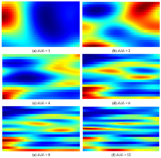
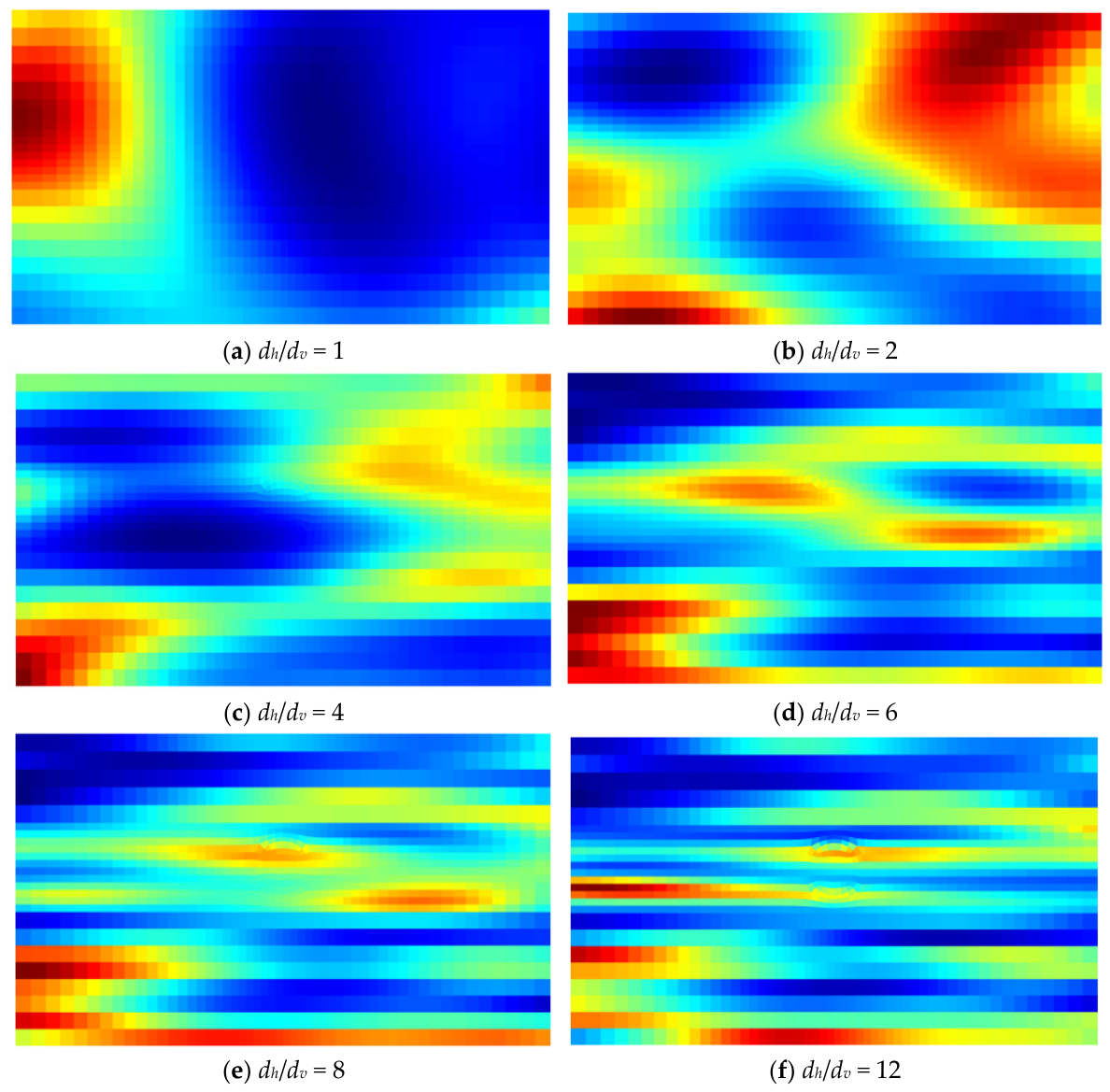
Figure 1 presents representative realizations, rather than finite-element verification results, of random fields generated with a common mean, coefficient of variation, vertical autocorrelation distance, and color scale. When d_h/d_v = 1, the horizontal and vertical autocorrelation distances are equal and the field is approximately isotropic. As d_h/d_v increases, zones with similar values become progressively elongated in the horizontal direction. The stronger banding in the last two panels is therefore the intended consequence of a larger horizontal correlation distance, not numerical divergence. Random-field generation was additionally checked by confirming that the sample statistics and directional correlation structure reproduced their prescribed inputs before coupling to the finite-element model.

$$\rho (\tau )=\exp (-{\displaystyle \frac{\left|{\tau }_x\right|}{d_h}}-{\displaystyle \frac{\left|{\tau }_z\right|}{d_v}})$$

(3)

Figure 1. Representative random-field realizations for different d_h/d_v values under a common mean, coefficient of variation, vertical correlation scale, and color scale; colors indicate relative normalized parameter values.

Building on the directional spatial structure, this study further introduces the rotation angle β to describe the deflection of the principal correlation direction. Since the bedding structure and depositional direction in natural deposits are often not aligned with the global coordinate system, coordinate rotation is required to reconstruct the principal correlation direction. The transformation can be expressed as follows:

$$\left[\begin{array}{c}{x}^{\prime }\\ z^{\prime }\end{array}\right]=\left[\begin{array}{cc}\cos \beta & \sin \beta \\ -\sin \beta & \cos \beta \end{array}\right]\left[\begin{array}{c}x\\ z\end{array}\right]$$

(4)

where (x′,z′) denotes the rotated local coordinate system, and β is the rotation angle of the principal correlation direction relative to the global horizontal axis.

In the rotated coordinate system, the spatial correlation function of the random field can be expressed as follows:

$$\rho ({\tau }_x^{\prime },{\tau }_z^{\prime })=\exp \left[-\sqrt{{\left({\displaystyle \frac{{\tau }_x^{\prime }}{d_h}}\right)}^2+{\left({\displaystyle \frac{{\tau }_z^{\prime }}{d_v}}\right)}^2}\right]$$

(5)

where τ′_x and τ′_z denote the spatial separation distances in the rotated coordinate system.

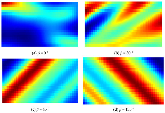
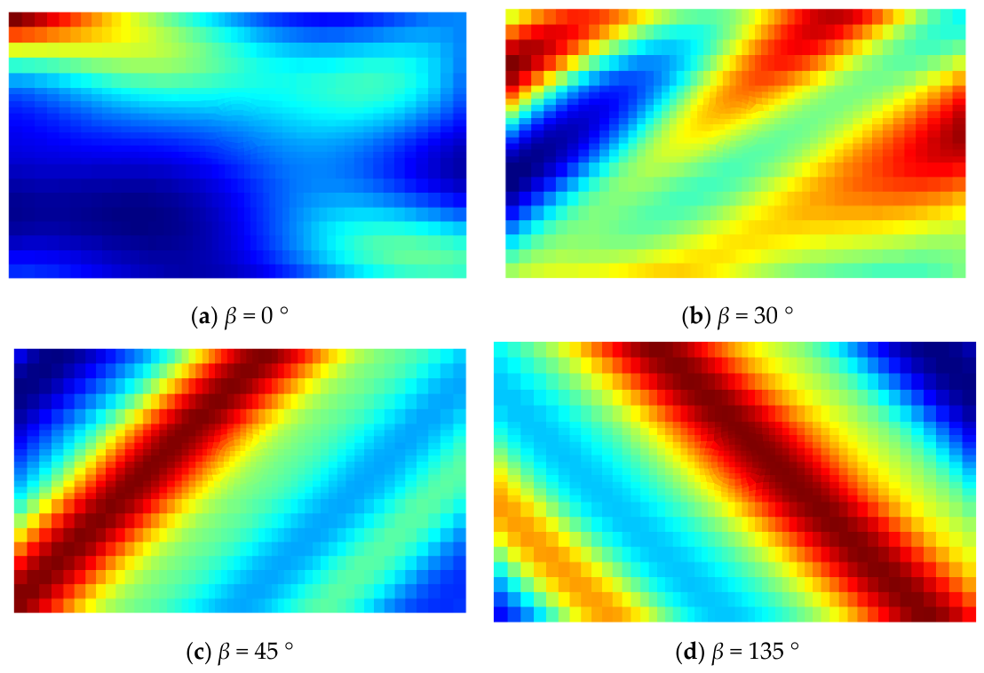
Figure 2 illustrates the principal correlation direction under different rotation angles β. According to Equation (4), β changes the angle between the principal correlation direction and the global coordinate system. When β = 0°, the principal direction is horizontal. As β increases to 30° and 45°, the elongated weak zones become inclined, changing their geometric relationship with the tunnel. At β = 135°, the inclination is opposite to that at β = 45°. Rotated principal directions are consistent with anisotropic spatial structures associated with bedding, deposition, and geological discontinuities [1,44,45]. Thus, β describes the orientation of the correlation structure. Within the adopted model, changing β alters how continuous weak zones intersect the excavation-affected region and is expected to influence settlement-trough asymmetry and peak location.

Figure 2. Schematic illustration of the principal correlation directions of random fields under different rotation angles; colors indicate relative normalized parameter values used to visualize directional continuity.

Accordingly, within the framework of this study, d_h/d_v mainly controls the intensity of morphological anisotropy of the settlement trough, whereas β mainly governs the preferential direction of settlement trough offset.

2.2. Non-Intrusive Random Finite Element Method Framework

To achieve efficient coupling between the random field and finite element analysis, this study adopts the non-intrusive random finite element method (non-intrusive RFEM). This method requires no modification to the underlying algorithm of the finite element solver. Instead, stochastic analysis is implemented through external random sample generation and parameter mapping. It therefore offers good generality and computational stability [19].

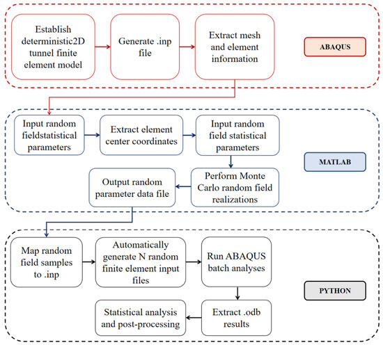
The RFEM analysis procedure used in this study is shown in Figure 3. Firstly, the covariance matrix of the random field is established using the spatial correlation function. The random variables are then mapped to the centroids of the finite element mesh elements using the midpoint discretization method. Next, Cholesky decomposition is used to generate random samples that satisfy the prescribed spatial correlation structure, and a large number of random field inputs are produced through Monte Carlo simulation. After the random parameters are assigned, automatic coupling between the random field model and the finite element solver is achieved through external parameter mapping. In this way, the ground surface settlement responses under different random realizations can be obtained. Finally, all stochastic simulation results are statistically analyzed to determine the mean settlement trough, settlement variability, and direction-dependent variation patterns.

Figure 3. Flowchart of the Non-intrusive Random Finite Element Analysis Procedure.

The random field is discretized using the midpoint method, in which the random-field value is evaluated at the centroid of each finite element. This method can effectively preserve the spatial correlation structure of the random field and reduce the discretization error. The covariance matrix can be defined as follows:

$$C_{\mathit{ij}}={\sigma }_X^2{\rho }_{\mathit{ij}}$$

(6)

where ρ_ij is the correlation coefficient between elements i and j.

The covariance matrix is then decomposed using Cholesky decomposition and can be expressed as:

C = LL^T

(7)

where L denotes a lower triangular matrix.

The random field sample can then be represented by:

X = Lξ + μ

(8)

in which ξ represents a standard normal random vector.

After the random field is generated, automatic mapping between the random parameters and the finite element model is implemented using Python 2.7.15 in the Abaqus/CAE 2020 scripting environment. A large number of stochastic simulations are then conducted through the Monte Carlo method, so that the statistical distribution characteristics of the settlement response can be obtained.

2.3. Settlement Evaluation Indices

Traditional settlement analyses generally focus on the maximum settlement Smax. Under a rotated anisotropic spatial structure, however, Smax alone cannot describe the direction-dependent morphology of the settlement trough. This study therefore also evaluates the peak offset probability P₀, peak offset distance Δx_max, slope of the line connecting the inflection points, and interquartile range. Together, these indices characterize settlement magnitude, offset stability, morphological asymmetry, and response dispersion.

Specifically, the maximum settlement S_max is used to quantify the magnitude of the tunneling-induced ground settlement response. The peak offset distance Δx_max describes the offset degree of the settlement trough peak relative to the tunnel centerline. The peak offset probability P₀ is used to evaluate the stability of the settlement trough offset, and it is defined as:

$$P_0={\displaystyle \frac{N_s}{N}}$$

(9)

where N_s is the number of random samples in which peak offset occurs, and s is the total number of simulations.

To further describe the left–right asymmetry of the settlement trough, this study adopts the slope of the line connecting the inflection points, namely the slope index, as a morphological evaluation index. According to the Gaussian settlement trough model proposed by Peck [1], the left and right inflection points of the settlement trough correspond to the standard deviation positions (±σ) of the Gaussian curve. Under an ideally symmetric condition, the two inflection points are equidistant from the tunnel centerline, and the slope index is equal to zero. When the rotated anisotropic random field leads to an uneven distribution of equivalent stiffness on both sides of the tunnel, the left and right inflection points shift asymmetrically. Therefore, the absolute value of the slope index increases, while the offset direction depends on the spatial orientation of the continuous weak zone relative to the tunnel axis. Hence, the slope index can quantitatively reflect the driving effect of the rotated anisotropic spatial structure on the asymmetric evolution of the settlement trough from a morphological perspective. It also serves as an effective supplement to the peak offset distance Δx_max and the peak offset probability P₀.

In addition, the interquartile range (IQR) is used to describe settlement dispersion. Because the IQR spans the 25th to 75th percentiles, it provides a robust measure of the central spread and is less sensitive to isolated extreme realizations than the full range. The IQR is calculated as follows:

IQR = Q₃ − Q₁

(10)

where Q₁ and Q₃ represent the first quartile, namely the 25th percentile, and the third quartile, namely the 75th percentile, of the ground surface settlement responses obtained from multiple random-field simulations, respectively. The IQR, defined in Equation (10), quantifies the spread within the central 50% of the settlement-response distribution. It can effectively reduce the influence of extreme values and therefore serves as a robust statistical measure of settlement uncertainty. On this basis, the statistical envelope is further constructed using the pointwise 5th and 95th percentiles of the settlement curves obtained from multiple random-field simulations. This envelope is used to describe the spatial dispersion range of ground surface settlement responses at different transverse positions and the directional expansion characteristics of the statistical settlement trough envelope.

3. Numerical Model and Validation

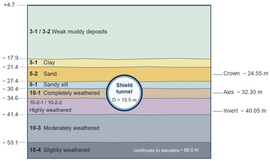
To validate the numerical procedure for tunneling-induced ground settlement, the Shenzhen Mawan Subsea Tunnel Project [51] was selected as the engineering case. Figure 4 presents the engineering geological profile along the validation section, redrawn from the project investigation data. The boreholes show the spatial variation in stratigraphy, and the two red lines indicate the upper and lower boundaries of the tunnel alignment. The subsequent numerical validation uses a representative two-dimensional plane-strain section and the parameters listed in Table 1. The site parameters in Table 1 span weak muddy deposits to weathered rock: elastic modulus ranges from 1.5 to 6000 MPa, cohesion from 3 to 45 kPa, friction angle from 0.5 degrees to 43 degrees, and Poisson’s ratio from 0.23 to 0.42. This range reflects the strong stratigraphic contrast of the project-based deterministic dataset. The Poisson’s ratios of 0.41–0.42 apply only to saturated weak muddy layers and approximate a nearly incompressible short-term response; deeper sands and weathered rocks use lower values. These project inputs should not be interpreted as universal values or as the parameter set for the idealized model in Section 4.

Figure 4. Representative transverse geological cross-section of the engineering validation section.

Table 1. Soil parameter values used in the engineering validation stage.

Layer	Soil Types	Elevation (m)	γ/(kN•m−3)	φ/(°)	C (kPa)	ν	E (MPa)
3-1	Muddy clay	−17.9	15.5	2.5	10	0.42	1.5
3-2	Muddy clay	−17.9	16.6	0.5	5	0.41	2
5-1	Clay	−21.4	19	18	30	0.32	15
5-2	Sand	−27.4	20	32	0	0.30	18
8-1	Sandy silt	−30.4	19	20	22	0.32	20
10-1	Completely weathered rock	−34.6	19.5	22	30	0.29	70
10-2-1	Highly weathered rock	−41.4	22	28	35	0.28	120
10-2-2	Highly weathered rock	−41.4	22.7	33	38	0.28	130
10-3	Medium weathered rock	−53.1	25	39	200	0.27	1300
10-4	Slightly weathered rock	−88	26	43	700	0.26	6000

Note: The second column reports elevation relative to the project datum. The Poisson’s ratios and low friction angles assigned to weak muddy layers 3-1 and 3-2 are equivalent Mohr–Coulomb inputs compiled from the project investigation dataset used in this study. Layers 3-1/3-2 and 10-2-1/10-2-2 occur as local interbeds at the same nominal boundary elevation and are grouped accordingly in Figure 4. Two decimal places are retained for Poisson’s ratio only to reproduce the numerical input file and do not imply measurement accuracy to two decimal places.

A two-dimensional plane-strain finite element model was established based on the engineering geological data. The soil was simulated using the Mohr–Coulomb constitutive model. The model parameters were determined according to the engineering investigation data and relevant studies, as listed in Table 1. Tunnel excavation was simulated using the stress release method, which can be expressed as:

F = (1 − λ)F₀

(11)

where F₀ is the initial ground stress, F is the residual load after excavation, and λ is the stress-release coefficient. In this study, λ = 0.65 was selected by calibrating the computed settlement trough against the monitoring profile used for validation. It is therefore a model-calibration parameter for the present two-dimensional equivalent-excavation analysis rather than a universally applicable material constant.

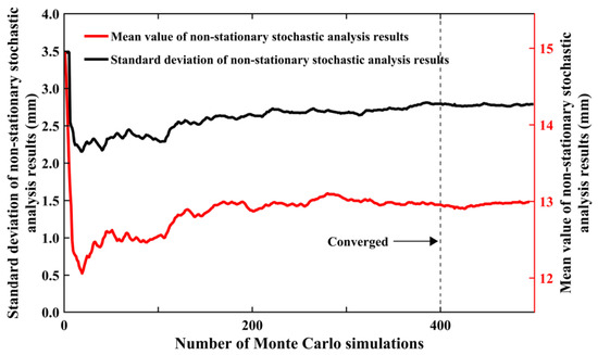
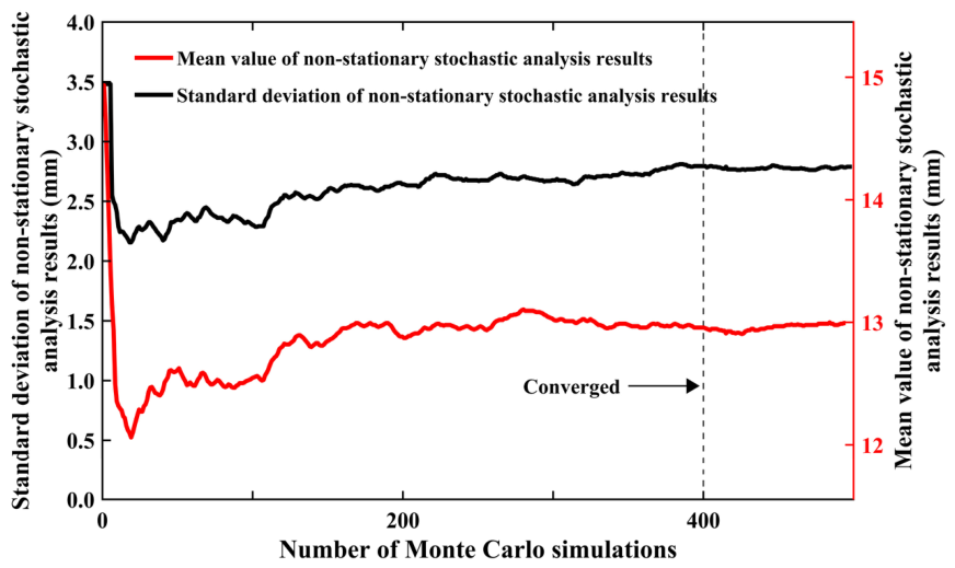
Before interpreting the RFEM results, the stability of the first two response moments was examined using the running mean and running standard deviation of maximum ground surface settlement (Figure 5). Both curves become comparatively stable by 400 realizations, so this sample size was adopted consistently for comparisons among parameter cases. This check supports comparison of the mean and standard deviation but is not a formal proof of convergence for rare-event tails. Probabilities and extreme quantiles based on 400 realizations retain sampling uncertainty; they are therefore interpreted as comparative indicators within the tested cases rather than exact tail estimates.

Figure 5. Monte Carlo convergence analysis curves.

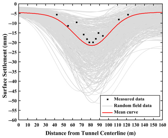
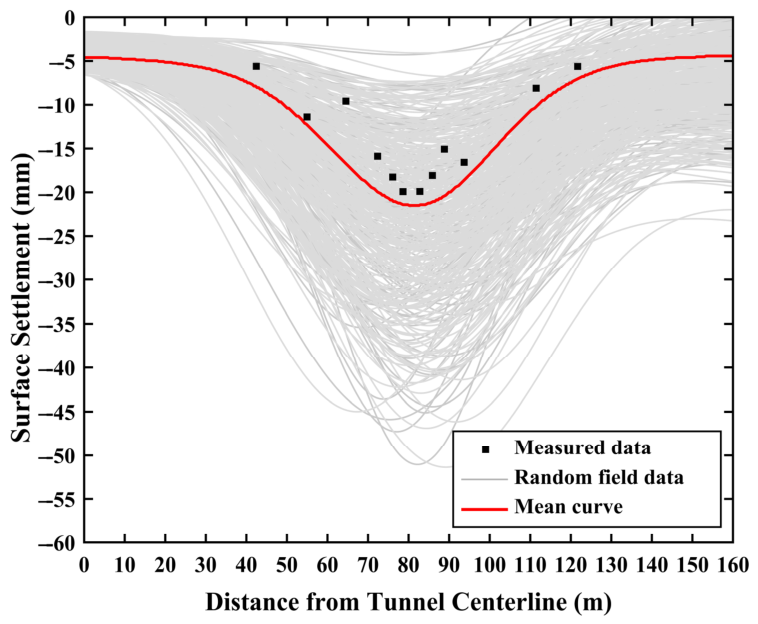
Figure 6 compares the numerical simulation results with the field monitoring data. The simulated mean reproduces the measured trough location and overall width, while the 5th–95th percentile envelope is intentionally broad because it propagates the prescribed spatial variability. The envelope should not be read as a deterministic prediction interval for every field observation. Its width also reflects modeling simplifications: the analysis is two-dimensional and plane-strain, uses a basic Mohr–Coulomb elastoplastic law and equivalent stress release, and does not explicitly reproduce three-dimensional face effects, detailed construction sequences, small-strain stiffness degradation, or parameter cross-correlation. The comparison therefore supports use of the model for mechanism-oriented trends and probabilistic bounds, but not exact site-specific quantitative prediction.

Figure 6. Comparison of measured ground surface settlement and RFEM model simulation results.

4. Comparative Effects of Different Random Soil Parameters

This section additionally investigates the effects of different random parameters on the ground surface settlement response induced by single-line tunnel excavation in soils with rotated spatial variability. To identify the independent contribution of each soil parameter, a parametric analysis is conducted. Under the condition of β = 45° and d_h/d_v =24/6, the elastic modulus E, cohesion c, and internal friction angle φ are separately treated as random variables. The settlement responses under different coefficients of variation are then compared using several indices, including the statistical settlement envelope, maximum settlement S_max, statistical distribution characteristics, and settlement-trough offset probability. The analysis in greater depth reveals the differences in the effects of different random parameters on the settlement magnitude, spatial dispersion, and uncertainty of ground surface settlement.

4.1. Random Field Model

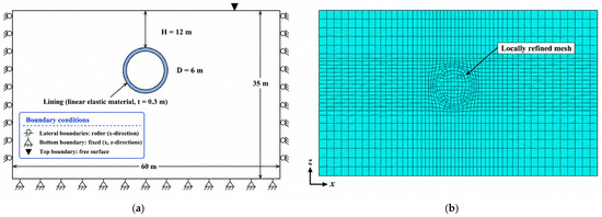
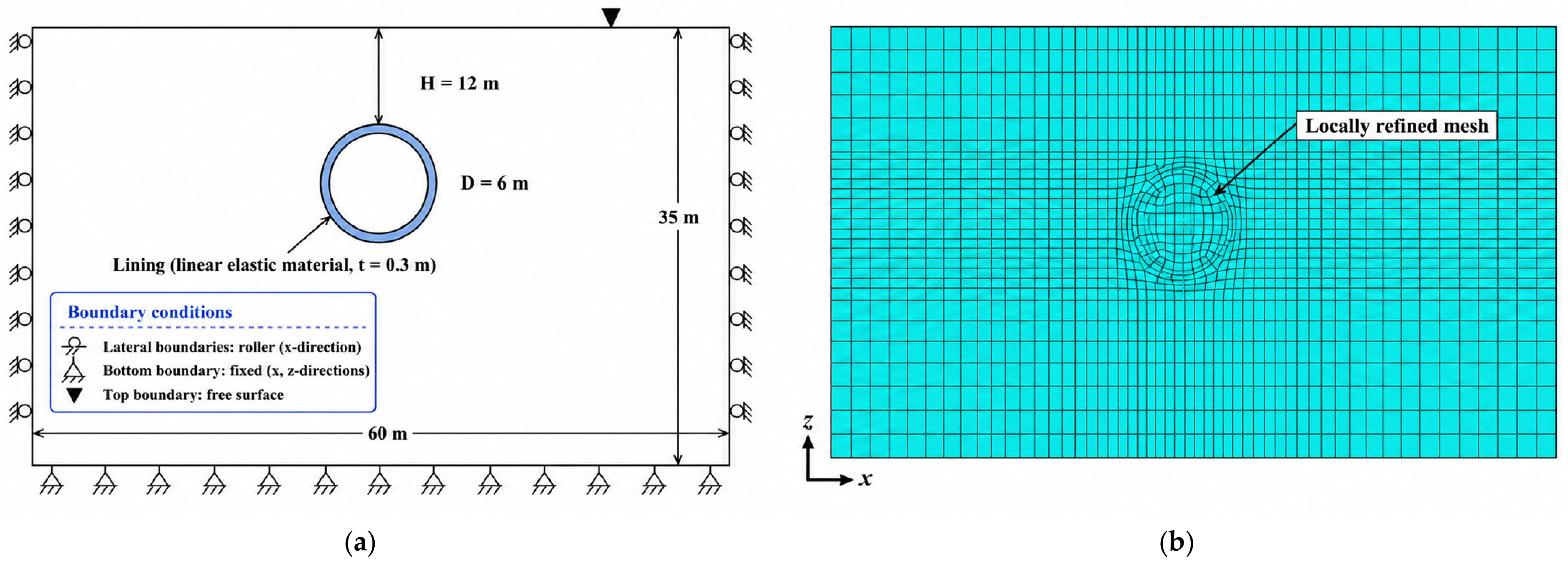
Figure 7 presents the geometry, boundary conditions, and schematic finite-element mesh of the two-dimensional random finite-element model. The domain is 60 m wide and 30 m deep. The tunnel has outer and inner diameters of 6.0 and 5.4 m, respectively, corresponding to a lining thickness of 0.3 m, and its center is located 15 m below the ground surface. The mesh is locally refined around the tunnel and within the excavation-affected zone to resolve the strong displacement and stress gradients. The model width is ten times the tunnel outer diameter, which limits the influence of the lateral boundaries. Horizontal and vertical displacements are constrained at the bottom boundary, the lateral boundaries are restrained normal to the boundary, and the ground surface is free.

Figure 7. Geometry, boundary conditions, and finite-element mesh of the two-dimensional RFEM model: (a) overall model dimensions and boundary conditions; (b) locally refined finite-element mesh around the tunnel.

Unlike the multilayer project model used for engineering validation in Section 3, the mechanism-oriented analyses in Section 4 employ an idealized homogeneous soft-soil domain so that the effects of spatial variability and rotated anisotropy can be isolated from stratigraphic contrasts. The soil is represented by a Mohr–Coulomb model with mean parameters E = 12 MPa, c = 13 kPa, φ = 8.5°, and ν = 0.30. These values define a controlled sensitivity model and are not averages of Table 1. The lining is linear elastic with an equivalent Young’s modulus of 15 GPa (15,000 MPa). The value of 15 MPa previously shown in Table 2 was a unit error; the numerical analyses used 15 GPa. Tunnel excavation is simulated using a stress-release coefficient of 0.65. The high Poisson’s ratios in two shallow validation layers are not transferred to this idealized model.

Table 2. Physical and mechanical parameters used in the idealized homogeneous parametric model.

Medium	Material	Thickness d (m)	γ/(kN•m−3)	φ (°)	c (kPa)	ν	E (MPa)
Soil	Elastic-perfectly plastic	-	18	8.5	13	0.3	12 (mean)
Lining	Linear elastic	0.3	24	-	-	0.2	15,000

The one-at-a-time design used below deliberately treats E, c, and phi as independent random inputs while holding the remaining parameters fixed, thereby isolating their marginal effects. This assumption does not reproduce the physical covariance between cohesion and friction angle, nor the dependence of E, n_u, c, and φ on strain level and stress path. Consequently, the results should be interpreted as controlled sensitivity comparisons. Correlated multivariate random fields and strain-dependent or small-strain constitutive models are required for site-specific quantitative prediction and are identified as priorities for future work.

4.2. Settlement Uncertainty Characteristics of Different Random Parameters Under Rotated Anisotropic Spatial Structures

To investigate the influence of the spatial variability of different random parameters on the ground surface settlement response at a deeper level, random field models are established under different E-cov, c-cov, and φ-cov conditions. The corresponding statistical results of ground surface settlement are obtained based on 400 random realizations. Table 3 lists the basic parameter settings used in the random field simulations.

Table 3. Random-field parameters used in the idealized homogeneous soft-soil model.

Parameter	Mean Value	COV	β (°)	dh/dv
Elastic modulus E (MPa)	12	0.1, 0.2, 0.3, 0.4, 0.5	45°	4
Cohesion c (kPa)	13	0.15, 0.2, 0.25	45°	4
Friction angle φ/(°)	8.5	0.05, 0.075, 0.1	45°	4

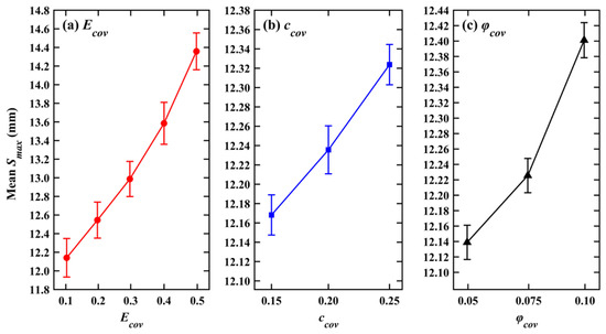
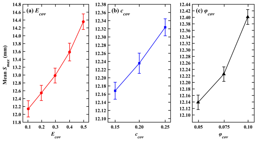
Figure 8 shows the mean maximum settlement Smax when E, c, and φ are varied separately. Increasing E-cov from 0.1 to 0.5 raises mean Smax from approximately 12.1 to 14.4 mm. Under the adopted lognormal model, a larger E-cov at fixed arithmetic mean increases the occurrence of localized low-stiffness zones within the excavation-affected region, reducing effective ground stiffness. By contrast, Smax increases only from approximately 12.17 to 12.33 mm over the tested c-cov range, and the change under the φ-cov cases is also much smaller than for E-cov. In these simulations, the response remains primarily deformation-controlled rather than governed by extensive shear yielding, so settlement magnitude is more sensitive to stiffness variability than to the tested strength-parameter variability. This interpretation is limited to the adopted model, mean values, and COV ranges and should not be generalized to failure-dominated conditions.

Figure 8. Variation in the mean S_max under different random parameter cases.

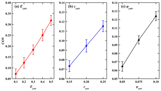
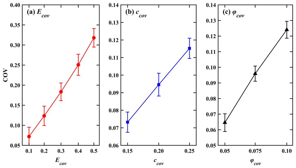
Figure 9 summarizes the response COV under the tested random-parameter cases. For E, five input levels show a strong monotonic increase in response variability, reaching approximately 0.32 at E-cov = 0.5. For c and phi, only three discrete levels were evaluated; these points indicate increasing trends over the tested ranges but are insufficient to establish a globally linear functional relationship. The wider uncertainty bars at larger input COV represent stronger propagation of input variability into the response. They do not, by themselves, demonstrate numerical instability. Because 400 realizations primarily stabilize the first two moments, the uncertainty of high-variability cases and tail estimates must still be acknowledged.

Figure 9. Coefficient of variation in settlement under different random parameter cases.

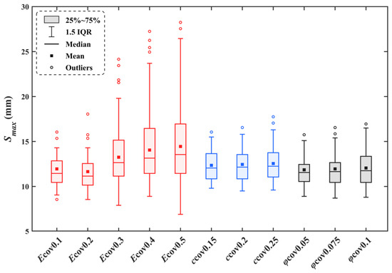
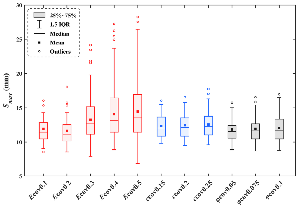
Figure 10 shows the boxplot distributions of Smax at β = 45 degrees and d_h/d_v = 4. The IQR and upper-tail spread increase with E-cov and, more moderately, with the tested c-cov and φ-cov levels. These boxplots corroborate the monotonic trends in Figure 9 within the sampled points, but they do not establish strict linearity outside those ranges. The larger spread at high input COV is physically consistent with uncertainty propagation; combined with the finite Monte Carlo sample, it also means that extreme observations and tail probabilities should be interpreted cautiously.

Figure 10. Boxplots of S_max under different random soil parameters.

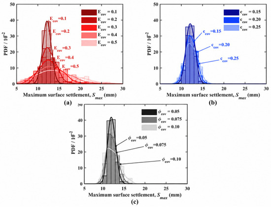
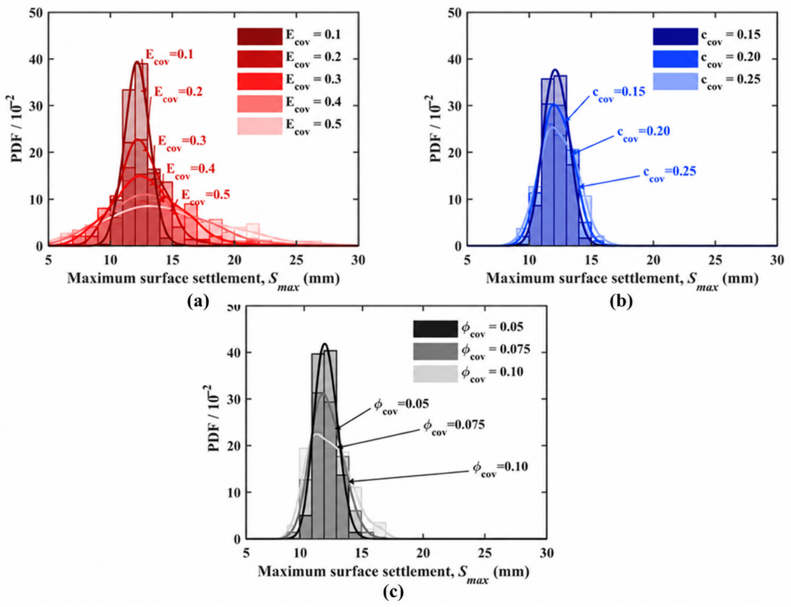
Figure 11 presents the probability density function (PDF) curves of the maximum ground surface settlement S_max under different random parameter cases. Figure 11a indicates that, as E-cov increases from 0.1 to 0.5, the PDF curve gradually changes from a sharp and narrow profile concentrated near 12 mm to a broader and flatter profile extending toward the larger settlement range. When E-cov = 0.1, the PDF peak is high, and the distribution is concentrated. When E-cov = 0.5, the peak value decreases markedly, and the probability in the right tail increases significantly. According to the parameterization characteristics of the lognormal distribution, an increase in the input COV leads to a larger logarithmic standard deviation, which further expands the width of the output response distribution. This is quantitatively consistent with the evolution of the PDF curve profile shown in Figure 11a. By contrast, the PDF curves under the c-cov and φ-cov cases in Figure 11b,c show much smaller variations. The peak locations remain relatively stable even when the randomness increases, indicating that the randomness of strength parameters affects the settlement distribution indirectly through the development of the plastic zone. Its influence on the PDF curve profile is weaker than the direct linear transmission effect of the elastic parameter. Among the strength parameters, the PDF curve profile broadening under the φ-cov case is slightly greater than that under the c-cov case. This is consistent with the physical mechanism by which cohesion and internal friction angle contribute differently to the shear failure envelope in the Mohr–Coulomb criterion. Nevertheless, both parameters play a secondary role in controlling the overall distribution shape.

Figure 11. Probability density function (PDF) curves of Smax under different coefficients of variation: (a) E-cov; (b) c-cov; and (c) φ-cov.

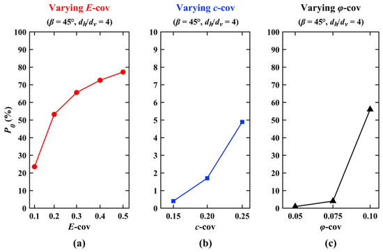
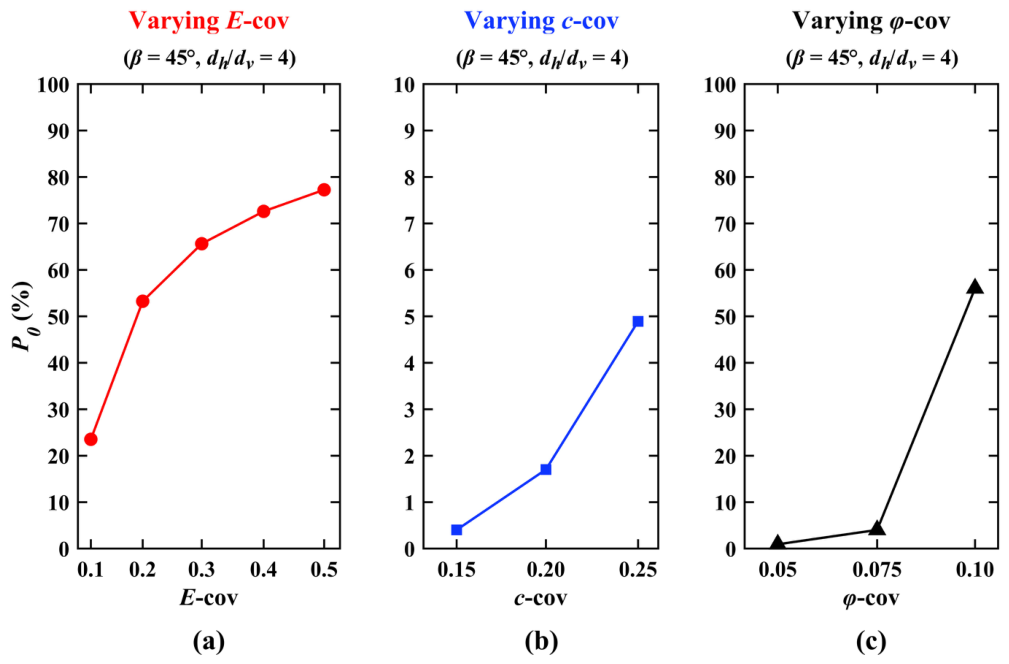
Figure 12 presents the variation in the peak offset probability P₀ under different random parameter cases. Figure 12a indicates that as E-cov increases from 0.1 to 0.5, P₀ continuously increases from approximately 24% to about 77%. This is because, under the rotated anisotropic random field condition with β = 45°, continuous low-stiffness zones tend to extend along the principal correlation direction, namely the 45° direction. When E-cov is relatively high, the probability of lower extreme values in the low-stiffness zones increases, and local stiffness heterogeneity becomes more evident. Such stiffness heterogeneity intensifies the difference in excavation-induced displacement responses between the two sides of the tunnel. Consistent with random-field tunneling analyses [29,50], a non-uniform stiffness distribution can shift the maximum-settlement location toward the lower-stiffness side, thereby increasing the likelihood of an asymmetric settlement trough. In contrast, under the c-cov case in Figure 12b, P₀ remains at a low level, and the increase in offset probability is limited even when COV increases to 0.25. In Figure 12c, P₀ increases markedly when φ-cov reaches 0.1, indicating that when the coefficient of variation in the internal friction angle exceeds 0.075 or a certain critical value, the randomness in the propagation direction of the local plastic zone increases. This may induce an asymmetric offset of the settlement trough, but its overall influence remains weaker than that under the E-cov case. Overall, the stiffness parameter E affects the offset probability by directly controlling the magnitude of ground deformation, whereas the strength parameters c and φ act through indirect changes in the development path of the plastic zone. Within the parameter ranges considered in this study, the former has a more significant effect.

Figure 12. Peak offset probability under varying (a) E-cov; (b) c-cov; and (c) φ-cov.

5. Directional Evolution of Settlement Troughs Under Rotated Anisotropic Spatial Structures

This section further investigates the influence mechanism of rotated anisotropic spatial structures on the directional evolution of settlement troughs. To identify the independent and combined effects of the rotation angle β and the autocorrelation distance ratio d_h/d_v, rotated anisotropic random field models are established under different β and d_h/d_v cases. Based on random finite element analysis and Monte Carlo simulations, several indices are systematically compared under different working cases, including the statistical envelope of the settlement trough, the maximum settlement offset Δx_max, the offset probability P₀, the slope index, and the settlement trough width. The analysis aims to reveal how the orientation of anisotropic spatial correlation governs the asymmetric trough expansion, directional offset, and uncertainty evolution.

5.1. Settlement Envelopes and Morphological Evolution

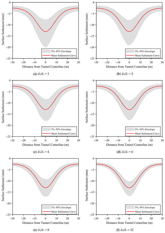
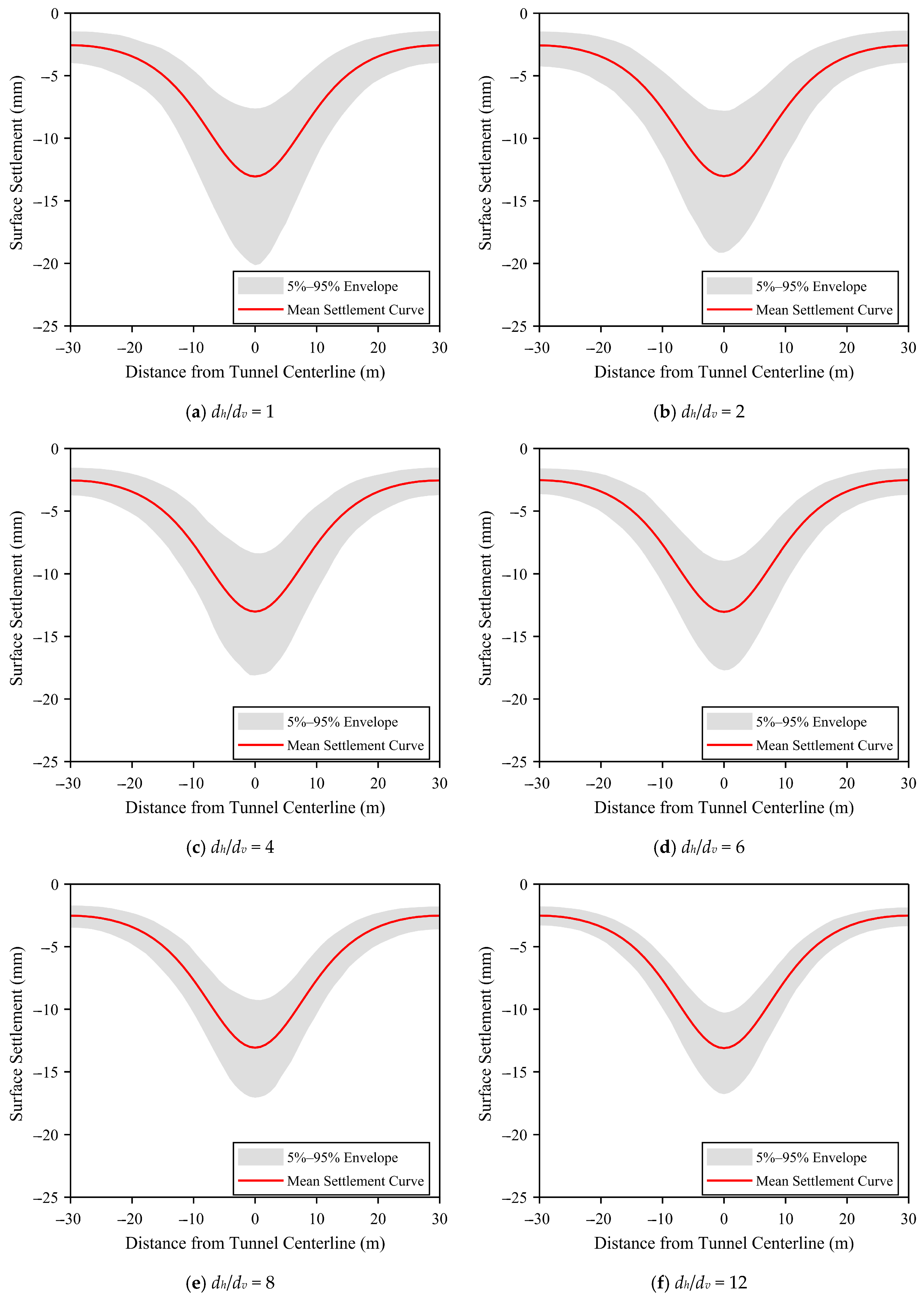
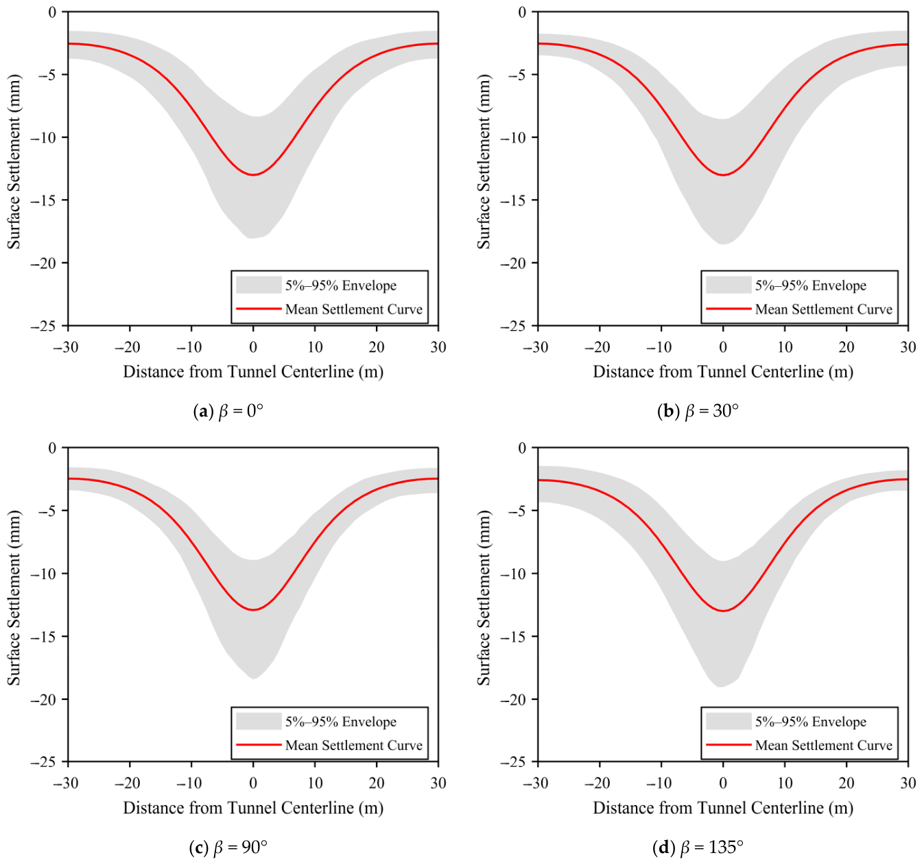
To investigate the influence of the autocorrelation-distance ratio on settlement-trough morphology without introducing directional bias, random-field models with d_h/d_v = 1, 2, 4, 6, 8, and 12 were established at β = 0 degrees. Statistical settlement envelopes were obtained from 400 realizations for each case, as shown in Figure 13. The six panels have been regenerated from their corresponding original datasets.

Figure 13. Corrected statistical envelopes of settlement troughs at β = 0 degrees for d_h/d_v = 1, 2, 4, 6, 8, and 12.

Figure 13 presents the corrected statistical envelopes at β = 0 degrees. The ensemble-mean curves remain nearly symmetric because the principal correlation direction is horizontal and aligned with the symmetric model geometry. Increasing d_h/d_v makes soil-property zones laterally more coherent, changes the effective number and extent of weak or stiff zones intersecting the excavation influence area, and modifies both trough width and response dispersion. The panels are therefore distinct even though their mean curves retain similar symmetry. These results concern coherence and morphological variability; they should not be interpreted as a universal variance-reduction law for every response metric.

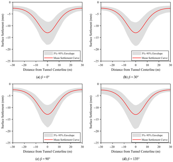
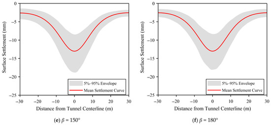
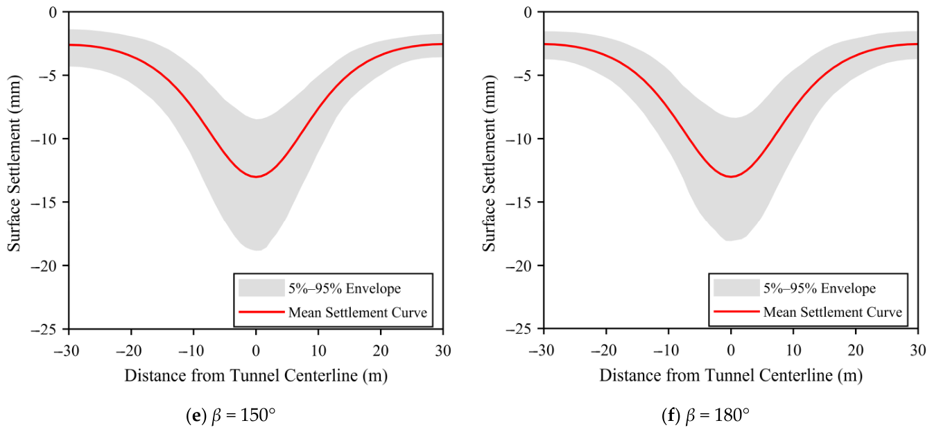
To further investigate the influence of the rotation angle, Figure 14 presents corrected statistical envelopes at d_h/d_v = 4 for β = 0, 30, 90, 135, 150, and 180 degrees. Each panel has been regenerated from its corresponding original dataset. The mean curves remain single-peaked, whereas the envelope shape and left–right dispersion vary with orientation because rotation changes how elongated weak and stiff zones intersect the excavation influence area.

Figure 14. Corrected statistical envelopes of settlement troughs at d_h/d_v = 4 for different principal-direction angles beta.

The statistical envelope morphology differs among the β cases. When β = 0° and 180°, the principal correlation direction is horizontal and the envelopes remain comparatively symmetric. From 30° to 90°, elongated weak and stiff zones intersect the excavation-affected region at different orientations, so the two sides do not sample equivalent spatial patterns in individual realizations. Among the tested cases, the envelope is widest at β = 90°, where vertically oriented continuous zones intersect a larger portion of the overburden above the tunnel and produce the greatest response dispersion in this model. When β changes further to 135° and 150°, the asymmetry decreases. The response is therefore non-monotonic and angle-sensitive; the β = 90° maximum is specific to the present geometry, boundary conditions, and random-field parameters rather than a universal rule.

5.2. Morphological Anisotropy Controlled by d_h/d_v

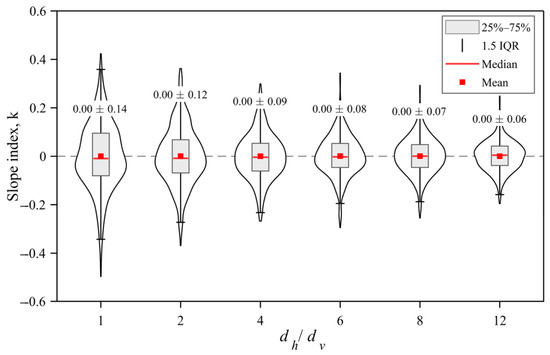
To further quantify the morphological evolution of the settlement trough, the slope index, defined as the gradient of the line connecting the left and right inflection points, is introduced to characterize trough asymmetry. Figure 15 presents the statistical distribution of the slope index under different d_h/d_v cases.

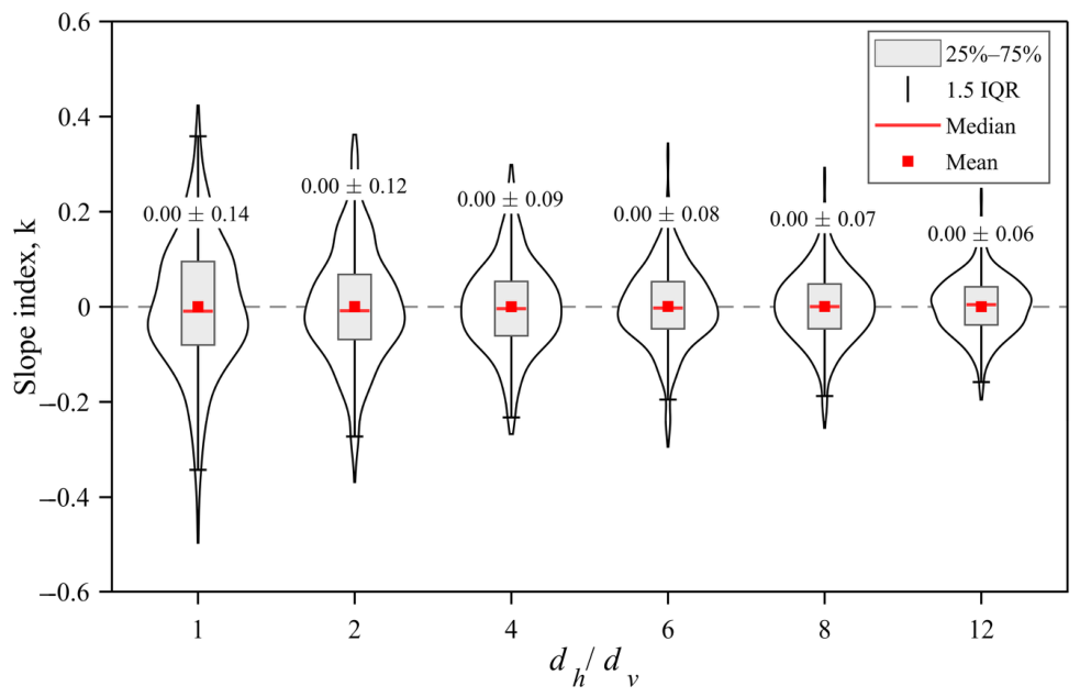
Figure 15. Slope index distributions under different d_h/d_v cases.

As shown in Figure 15, the mean slope index remains close to zero across all dh/dv cases, indicating that increasing dh/dv does not create a systematic left- or right-side bias when β = 0°. This is consistent with the symmetric Gaussian-type settlement trough represented in classical tunneling-settlement models [1,2]. In the present model, horizontally aligned weak and stiff zones occur with equal probability on the two tunnel flanks in the ensemble sense, so no persistent directional preference appears in the mean trough morphology.

Figure 15, rather than Figure 13 and Figure 14, quantifies the decrease in slope-index standard deviation from 0.14 to 0.06 as d_h/d_v increases from 1 to 12. This result should not be interpreted as the classical Vanmarcke variance-reduction effect caused by an averaging domain becoming large relative to the correlation scale. A larger horizontal correlation distance actually reduces the number of effectively independent horizontal zones. For the present slope index, the narrower distribution arises because increased lateral coherence causes the left and right inflection points to move more coordinately, even though other response measures, including settlement amplitude or envelope width, may show greater dispersion. The interpretation is therefore response-specific and consistent with local-average theory.

These results collectively demonstrate that d_h/d_v exerts its primary influence on trough morphology not through the mean slope index but through the dispersion of asymmetric responses across realizations. A larger horizontal correlation scale stabilizes the average trough shape while simultaneously constraining the range of morphological variability, an effect that is distinct from and complementary to the directional control exerted by β on the preferential offset direction.

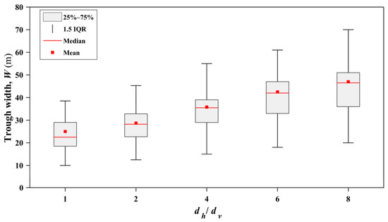
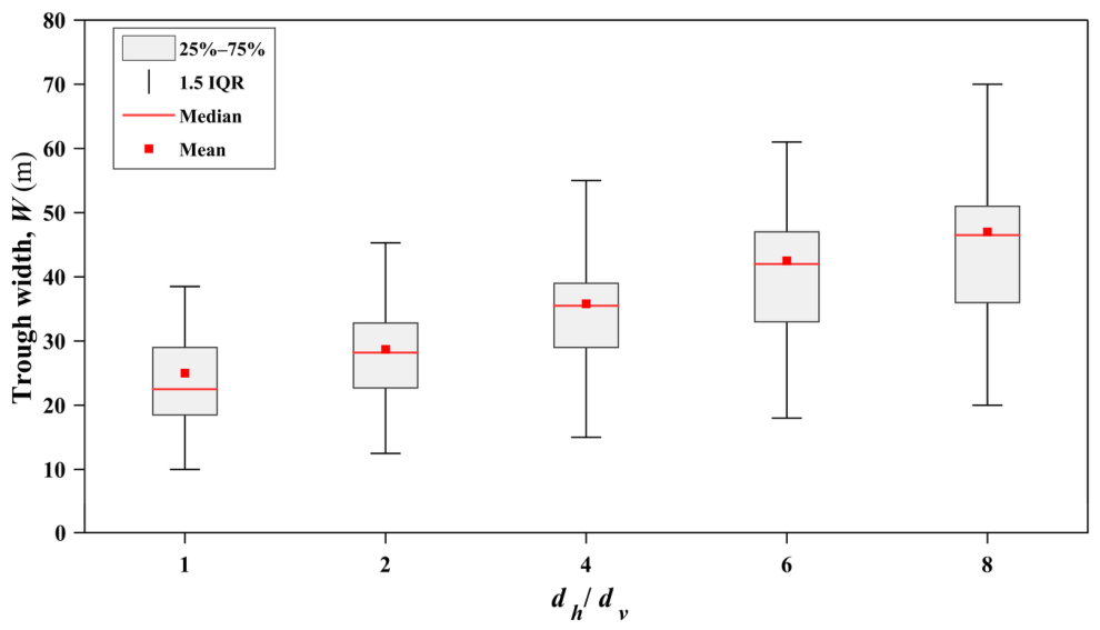
Figure 16 illustrates the boxplot statistics of settlement trough width W under different d_h/d_v cases. As shown in the figure, as d_h/d_v increases from 1 to 8, the mean settlement trough width increases markedly from approximately 25 m to about 47 m, with an increase of nearly 90%. According to the settlement trough width parameter proposed by O’Reilly and New [2], the settlement trough width in homogeneous ground is mainly governed by the cover depth. Under anisotropic random field cases, however, the continuous extension of horizontal low-stiffness zones directly enlarges the transverse extent of the settlement zone, which is equivalent to introducing an additional settlement expansion beyond the range predicted for homogeneous ground. As d_h/d_v increases, the spatial scale of horizontally continuous weak zones gradually extends beyond the settlement influence range defined by the Peck model, causing the actual settlement trough width to systematically exceed the homogeneous prediction. Moreover, the width increase becomes more pronounced under the d_h/d_v = 6 and 8 cases, showing a certain nonlinear trend. This indicates that when the horizontal autocorrelation distance exceeds the radius of the tunnel excavation-affected zone, approximately 2 to 3 times the tunnel diameter, the dominant role of the principal correlation direction in controlling the lateral expansion of the settlement trough becomes more evident. It can also be observed that the dispersion range of the boxplot expands simultaneously with increasing d_h/d_v. The evident increase in the upper-tail range at high d_h/d_v values indicates the occurrence of extreme settlement trough widths in some cases, which provides important engineering implications for evaluating the influence range of ground surface settlement.

Figure 16. Boxplot statistics of settlement trough width under different d_h/d_v cases.

5.3. Directional Control of Settlement Trough Offset by β

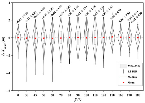
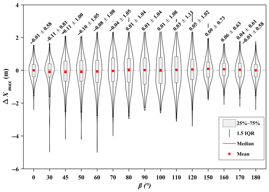
Figure 17 presents the statistical distribution characteristics of the maximum settlement position offset distance Δx_max under different rotation angles β. The results indicate that the mean values of Δx_max under all cases are generally close to 0, suggesting that, in a statistical mean sense, the maximum settlement position is still mainly distributed near the tunnel centerline. This is consistent with the symmetric single-peak prediction of the Peck Gaussian settlement model. Rotated anisotropy does not cause a persistent unidirectional offset of the mean settlement peak.

Figure 17. Distribution of Δx_max under different β cases.

When β = 0° and 180°, the distribution of Δx_max is the most concentrated, with the smallest violin width and box height. This indicates that the spatial stability of the settlement peak is strongest under these two cases. According to the effect of the rotation angle, when β = 0° and 180°, the principal correlation direction is parallel to the global horizontal axis. The continuous low-stiffness zones extend horizontally, and the geometric probability of intersection between the weak zones and the two sides of the tunnel is symmetric. As a result, the random weak-stiffness zones are less likely to form a unilateral deformation-dominated mode. This also explains why the settlement trough envelope tends to remain more symmetric under these rotation angles.

As β changes to 45–120°, the principal correlation direction becomes inclined, and the sectional relationship between the continuous weak zones and the excavation-affected zone becomes increasingly asymmetric. Similar to the evolution pattern of the settlement trough envelope, the distribution range of Δx_max expands significantly, indicating an enhanced random fluctuation of the peak position. The standard deviation reaches its maximum near β = 80–110°. Based on the coordinate rotation transformation, when β falls within this range, the principal correlation direction of the random field forms the strongest asymmetric sectional relationship with the excavation-affected zone. The continuous weak zones pass through the two sides of the tunnel at a high inclination angle, leading to the largest fluctuation in the equivalent stiffness difference between the left and right ground in different random realizations. In some random realizations, the continuous weak zones are completely biased toward one side of the tunnel, which significantly amplifies the deformation response on that side and increases the probability of extreme settlement. This causes the statistical standard deviation of the settlement response to reach the highest level within this rotation-angle range. In addition, the mean value of Δx_max changes from negative to positive with increasing β, reflecting a systematic transition in the dominant offset direction as the principal correlation direction rotates. This transition is mainly caused by the geometric change in the relative position between the continuous weak zones and the tunnel axis in the rotated coordinate system.

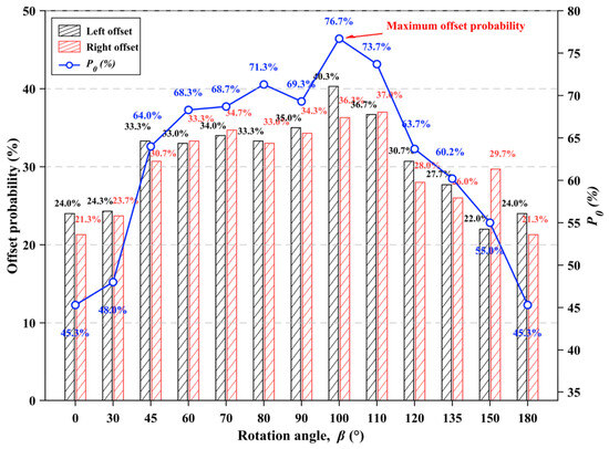
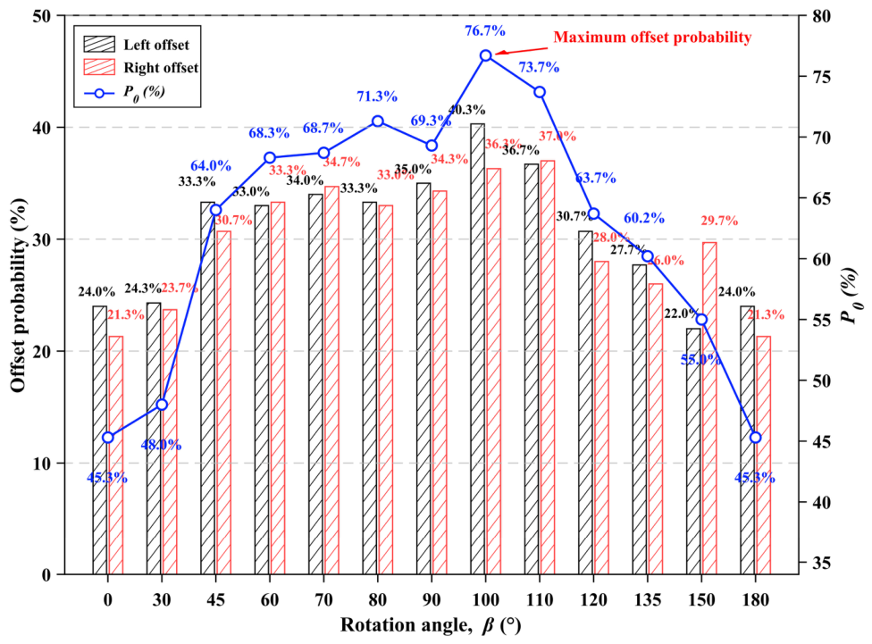
The combined distributions of the left-offset probability, right-offset probability, and overall peak offset probability P₀ under different rotation angles β are shown in Figure 18. The coordinated evolution of these three indices reveals the dual influence of the rotation angle on both the probability and preferential direction of maximum-settlement-location offset, thereby providing a directional complement to the preceding analyses of Δx_max and the slope index. The variation in P₀ with β confirms the conclusion drawn above. Specifically, P₀ increases continuously from 45.3% at β = 0° to a peak value of 76.7% at β = 100°, and then gradually decreases to 45.3% at β = 180°, which is identical to the value at β = 0°. This reflects the periodic symmetry associated with the coordinate rotation transformation. It is worth noting that P₀ remains above 68% over a relatively wide angular interval of β = 60° to 110°. This indicates that when the principal correlation direction rotates into this range, the continuous weak zones and the excavation-affected zone remain in a markedly asymmetric intersection pattern in the tunnel cross-section, so the probability of peak offset remains consistently high rather than being concentrated at a single angle.

Figure 18. Variation in leftward and rightward offset probabilities and overall peak offset probability under different β angles.

In terms of the allocation of left- and right-offset probabilities, the peak angles of the two probabilities differ by approximately 20°. The right-offset probability reaches its maximum value of 34.7% at β = 80°, whereas the left-offset probability attains its maximum value of 40.3% at β = 100°. This mismatch arises from the asynchronous evolution of the sectional relationship between the continuous weak zones and the two sides of the tunnel during the rotation of the principal correlation direction. As β increases from a small angle, the dominant intersection relationship of the continuous weak zones gradually shifts across the tunnel section, causing the peak of the left-offset probability to occur later than that of the right-offset probability. At β = 90°, the left-offset probability (35.0%) and the right-offset probability (34.3%) are very close, while P₀ has already reached a high value of 69.3%. This indicates that the offset risk is high under this case, whereas the directionality is the weakest. This is consistent with the previously observed maximum standard deviation of the slope index at β = 90°. Together, these results indicate that the uncertainty of settlement trough morphology is greatest at this angle, whereas the dominant offset direction is the least distinct. In contrast, under the β = 100° to 110° cases, the left-offset probability is systematically higher than the right-offset probability. Combined with the fact that P₀ reaches its highest level within this interval, this demonstrates that this angular range is characterized by both the highest offset risk and the most pronounced left-biased directionality. From an engineering perspective, for strata in which the principal correlation direction is around β = 100° to 110°, monitoring of ground surface settlement on the left side of the tunnel should be strengthened. By contrast, for strata with β ≈ 90°, monitoring points should be arranged uniformly on both sides of the tunnel, so as to avoid missing peak-offset events due to attention being focused on only one side.

5.4. Coupled Effects of β and d_h/d_v

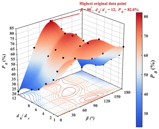
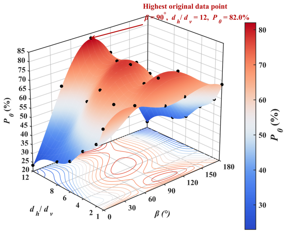
Figure 19 presents the three-dimensional response surface and corresponding contour plot of peak offset probability P₀ under the combined effects of rotation angle β and autocorrelation distance ratio d_h/d_v. P₀ exhibits a clearly coupled dependence on both β and d_h/d_v, confirming that the two parameters jointly exert significant synergistic control over peak offset probability.

Figure 19. Three-dimensional response surface of P₀ with respect to β and d_h/d_v.

When β = 0°, P₀ decreases monotonically with increasing d_h/d_v. As d_h/d_v increases, the horizontal scale of fluctuation expands and the spatial averaging effect of the soil parameter field in the horizontal direction is enhanced [13]. When the principal correlation direction is spatially symmetric with respect to the model geometry, this averaging effect causes the parameter distributions on both tunnel flanks to converge, progressively weakening the stochastic driving force for peak offset. When β rotates to intermediate angles, P₀ increases with d_h/d_v, as enlarging d_h/d_v continuously extends connected low-stiffness zones along the principal correlation direction, forming a wider asymmetric sectional relationship with the excavation-affected zone and raising the probability of unilateral dominant deformation. The highest P₀ among all original data points occurs at β = 90° and d_h/d_v = 12, where P₀ reaches 82.0%, as annotated in Figure 19. The response surface further reveals that the peak region of P₀ is broadly distributed across intermediate β values and large d_h/d_v, rather than being concentrated at a single combination, indicating that the amplifying effect of d_h/d_v on peak offset risk persists across a wide angular range when the principal correlation direction forms an asymmetric relationship with the tunnel.

The contour plot provides additional quantitative insight into the direction-dependent nature of the d_h/d_v effect. High-P₀ contours are concentrated in the combined range of intermediate rotation angles and large d_h/d_v, whereas low-P₀ contours cluster near β = 0° and 180° with large d_h/d_v, where the spatial averaging effect dominates and P₀ is suppressed to its lowest values. This directional reversal, in which the same increase in d_h/d_v raises P₀ under asymmetric β conditions but reduces it under symmetric ones, establishes that d_h/d_v and β cannot be evaluated independently. Their coupled effect is the governing determinant of peak offset probability in rotationally anisotropic ground.

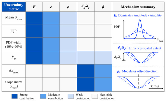
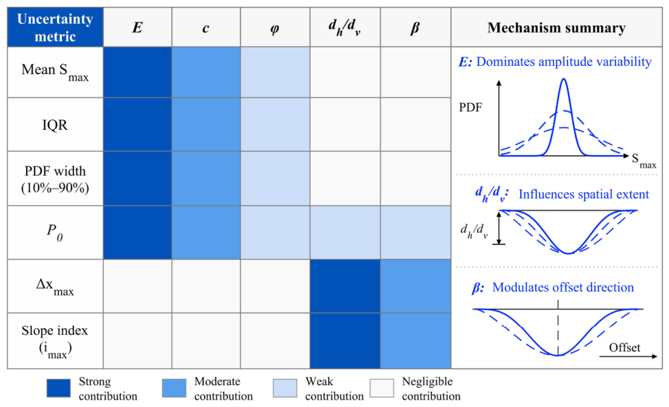
Figure 20 presents a comparative schematic of the relative contributions of elastic modulus E, autocorrelation distance ratio d_h/d_v, and rotation angle β to different settlement evaluation indices. The three factors exhibit clearly differentiated contribution patterns, corresponding to three distinct physical mechanisms.

Figure 20. Schematic diagram of the contributions of different random parameters to settlement uncertainty.

Elastic modulus E exerts strong contributions to mean S_max, IQR, and PDF width, reflecting its governing role in controlling settlement amplitude and statistical dispersion through the spatial distribution of stiffness. As the COV of lognormally distributed E increases, the probability of extremely low-stiffness zones rises systematically, amplifying the conversion from excavation-induced stress release to surface deformation. Regardless of ground anisotropy characteristics, the COV of E should therefore be treated as the primary investigation parameter for settlement amplitude uncertainty, with IQR and PDF tail exceedance probability serving as the core risk control indices.

The autocorrelation distance ratio d_h/d_v contributes most strongly to slope index and trough width, reflecting its role in governing the lateral continuity of low-stiffness zones. Once the lateral extension of these zones exceeds the settlement influence boundary predicted under homogeneous conditions, both effective trough width and left–right asymmetry increase systematically. When d_h/d_v is large, slope index and trough width should be incorporated into the evaluation framework alongside conventional settlement amplitude indices.

The rotation angle β contributes strongly to P₀ and Δx_max but negligibly to mean Smax, IQR, and PDF width, reflecting a mechanism that is geometric rather than statistical in nature. Instead of altering the parameter distribution, β regulates the asymmetry between connected weak zones and the two tunnel flanks by modifying the spatial orientation of the principal correlation direction, as illustrated in the mechanism schematic in Figure 20. When β lies within the intermediate angular range, P₀ and Δx_max should be adopted as the primary evaluation indices, and monitoring sections should be arranged asymmetrically on both tunnel flanks with closer spacing on the side of higher offset risk.

Taken together, under high-risk cases combining large d_h/d_v and intermediate β, the synergistic contributions of all three factors become most pronounced, and a multi-index evaluation framework incorporating mean S_max, IQR, PDF width, P₀, Δx_max, and slope index should replace single maximum settlement value as the basis for settlement risk classification.

6. Conclusions

This study establishes a non-intrusive rotationally anisotropic RFEM framework for tunneling-induced ground settlement analysis, in which the rotation angle β and autocorrelation distance ratio d_h/d_v are adopted as the primary parameters characterizing the directional random field structure. Based on 400 Monte Carlo realizations, the governing mechanisms of directional settlement trough evolution in anisotropic ground are systematically revealed from four perspectives: settlement magnitude, statistical dispersion, spatial stability of the settlement peak, and trough morphological asymmetry. The principal conclusions are as follows.

(1) Within the adopted lognormal parameter model and tested COV range, elastic-modulus variability is the dominant stochastic driver of settlement magnitude and dispersion. Increasing E-cov raises the occurrence of lower-tail stiffness realizations and increases mean Smax and response spread. This finding must not be extrapolated to vanishing stiffness or to deep stratigraphic units outside the calibrated parameter range. The present one-at-a-time analysis also neglects c-phi covariance and the strain dependence of E, nu, c, and phi; these effects require correlated multivariate fields and advanced constitutive models for quantitative site-specific assessment.

(2) The rotation angle beta governs the spatial stability of the settlement peak by changing how the principal correlation direction intersects the excavation influence zone. The mean peak offset remains close to zero because positive and negative offsets balance across realizations. At intermediate angles, however, the distribution widens: individual realizations show larger offsets to either side even though the ensemble mean remains near the tunnel centerline. Thus, near-zero mean offset does not imply low offset risk, and peak-offset probability is needed to characterize realization-level instability.

(3) The influence of d_h/d_v on peak-offset probability is direction-dependent. At β = 0 and 180 degrees, increasing horizontal coherence promotes coordinated left–right behavior and reduces peak migration. At intermediate orientations, elongated weak zones intersect the excavation influence area obliquely and increase asymmetric realization-level responses. The corrected envelope plots and slope-index statistics show that this mechanism is response-specific: lateral coherence can narrow the slope-index distribution while widening settlement envelopes or trough width. For the coupled case β = 90 degrees and d_h/d_v = 12, the peak-offset probability reaches approximately 82%.

In summary, elastic-modulus variability, d_h/d_v, and beta govern settlement magnitude and dispersion, lateral coherence, and spatial orientation, respectively. Maximum settlement alone is insufficient to characterize risk in rotated anisotropic ground; the settlement envelope, trough width, slope index, peak offset, and peak-offset probability should be considered together. The proposed framework is a mechanism-oriented probabilistic tool. Its quantitative application to a specific project requires site-calibrated correlation scales, statistically supported cross-correlations, strain-dependent constitutive behavior, construction-sequence representation, and larger samples when rare-event probabilities are required.

References

- Peck, R.B. Deep excavations and tunnelling in soft ground. In Proceedings of the 7th International Conference on Soil Mechanics and Foundation Engineering, Mexico City, Mexico, 25–29 August 1969; pp. 225–290. [Google Scholar]
- O’Reilly, M.P.; New, B.M. Settlements above tunnels in the United Kingdom: Their magnitude and prediction. In Proceedings of the Tunnelling ‘82 Symposium, Brighton, UK, 7–11 June 1982; pp. 173–181. [Google Scholar]
- Attewell, P.B.; Yeates, J.; Selby, A.R. Soil Movements Induced by Tunnelling and Their Effects on Pipelines and Structures; Blackie: Glasgow, UK, 1986. [Google Scholar]
- Mair, R.J.; Taylor, R.N.; Bracegirdle, A. Subsurface settlement profiles above tunnels in clays. Geotechnique 1993, 43, 315–320. [Google Scholar] [CrossRef] [Scilit]
- Mair, R.J.; Taylor, R.N. Bored tunnelling in the urban environment. In Proceedings of the 14th International Conference on Soil Mechanics and Foundation Engineering, Hamburg, Germany, 6–12 September 1997; pp. 2353–2385. [Google Scholar]
- Loganathan, N.; Poulos, H.G. Analytical prediction for tunneling-induced ground movements in clays. J. Geotech. Geoenviron. Eng. 1998, 124, 846–856. [Google Scholar] [CrossRef] [Scilit]
- Sagaseta, C. Analysis of undrained soil deformation due to ground loss. Geotechnique 1987, 37, 301–320. [Google Scholar] [CrossRef] [Scilit]
- Potts, D.M.; Addenbrooke, T.I. A structure’s influence on tunnelling-induced ground movements. Proc. Inst. Civ. Eng. Geotech. Eng. 1997, 125, 109–125. [Google Scholar] [CrossRef] [Scilit]
- Franzius, J.N.; Potts, D.M.; Burland, J.B. The response of surface structures to tunnel construction. Proc. Inst. Civ. Eng. Geotech. Eng. 2006, 159, 3–17. [Google Scholar] [CrossRef] [Scilit]
- Zhao, C.; Schmoedderich, C.; Barciaga, T.; Röchter, L. Response of building to shallow tunnel excavation in different types of soil. Comput. Geotech. 2019, 115, 103165. [Google Scholar] [CrossRef] [Scilit]
- Zhang, Z.G.; Zhang, M.X.; Jiang, Y.J.; Bai, Q.; Zhao, Q. Analytical prediction for ground movements and liner internal forces induced by shallow tunnels considering non-uniform convergence pattern and ground-liner interaction mechanism. Soils Found. 2017, 57, 211–226. [Google Scholar] [CrossRef] [Scilit]
- Lumb, P. The variability of natural soils. Can. Geotech. J. 1966, 3, 74–97. [Google Scholar] [CrossRef] [Scilit]
- Vanmarcke, E.H. Probabilistic modeling of soil profiles. J. Geotech. Eng. Div. 1977, 103, 1227–1246. [Google Scholar] [CrossRef] [Scilit]
- Vanmarcke, E. Random Fields: Analysis and Synthesis; MIT Press: Cambridge, MA, USA, 1983. [Google Scholar]
- Phoon, K.K.; Kulhawy, F.H. Characterization of geotechnical variability. Can. Geotech. J. 1999, 36, 612–624. [Google Scholar] [CrossRef]
- Phoon, K.K.; Kulhawy, F.H. Evaluation of geotechnical property variability. Can. Geotech. J. 1999, 36, 625–639. [Google Scholar] [CrossRef]
- Fenton, G.A.; Vanmarcke, E.H. Simulation of random fields via local average subdivision. J. Eng. Mech. 1990, 116, 1733–1749. [Google Scholar] [CrossRef] [Scilit]
- Fenton, G.A.; Griffiths, D.V. Bearing-capacity prediction of spatially random c-phi soils. Can. Geotech. J. 2003, 40, 54–65. [Google Scholar] [CrossRef] [Scilit]
- Fenton, G.A.; Griffiths, D.V. Risk Assessment in Geotechnical Engineering; Wiley: New York, NY, USA, 2008. [Google Scholar]
- Griffiths, D.V.; Fenton, G.A. Probabilistic slope stability analysis by finite elements. J. Geotech. Geoenviron. Eng. 2004, 130, 507–518. [Google Scholar] [CrossRef] [Scilit]
- Griffiths, D.V.; Huang, J.; Fenton, G.A. Influence of spatial variability on slope reliability using 2-D random fields. J. Geotech. Geoenviron. Eng. 2009, 135, 1367–1378. [Google Scholar] [CrossRef] [Scilit]
- Cho, S.E. Probabilistic assessment of slope stability that considers the spatial variability of soil properties. J. Geotech. Geoenviron. Eng. 2010, 136, 975–984. [Google Scholar] [CrossRef] [Scilit]
- Jiang, S.H.; Li, D.Q.; Zhang, L.M.; Zhou, C.-B. Slope reliability analysis considering spatially variable shear strength parameters using a non-intrusive stochastic finite element method. Eng. Geol. 2014, 168, 120–128. [Google Scholar] [CrossRef] [Scilit]
- Jiang, S.H.; Li, D.Q.; Cao, Z.J.; Zhou, C.-B.; Phoon, K.-K. Efficient system reliability analysis of slope stability in spatially variable soils using Monte Carlo simulation. J. Geotech. Geoenviron. Eng. 2015, 141, 04014096. [Google Scholar] [CrossRef] [Scilit]
- Li, D.Q.; Jiang, S.H.; Cao, Z.J.; Zhou, W.; Zhou, C.-B.; Zhang, L.-M. A multiple response-surface method for slope reliability analysis considering spatial variability of soil properties. Eng. Geol. 2015, 187, 60–72. [Google Scholar] [CrossRef] [Scilit]
- Mollon, G.; Dias, D.; Soubra, A.H. Probabilistic analyses of tunneling-induced ground movements. Acta Geotech. 2013, 8, 181–199. [Google Scholar] [CrossRef] [Scilit]
- Ali, A.; Lyamin, A.V.; Huang, J.; Cassidy, M. Undrained stability of a single circular tunnel in spatially variable soil subjected to surcharge loading. Comput. Geotech. 2017, 84, 16–27. [Google Scholar] [CrossRef] [Scilit]
- Hu, B.; Wang, C. Ground surface settlement analysis of shield tunneling under spatial variability of multiple geotechnical parameters. Heliyon 2019, 5, e02495. [Google Scholar] [CrossRef] [Scilit] [PubMed]
- Cheng, H.; Chen, J.; Li, J. Probabilistic analysis of ground movements caused by tunneling in a spatially variable soil. Int. J. Geomech. 2019, 19, 04019125. [Google Scholar] [CrossRef] [Scilit]
- Zhang, S.; Wang, Y.; Gao, Q.; Ma, X.; Zhou, H.; Wang, Z. Probabilistic analysis of ground settlement induced by tunnel excavation in multilayered soil considering spatial variability. Comput. Geotech. 2024, 165, 105951. [Google Scholar] [CrossRef] [Scilit]
- Zhou, X.; Wang, T. Uncertainty analysis and risk assessment for variable settlement properties of building foundation soils. Buildings 2025, 15, 2369. [Google Scholar] [CrossRef] [Scilit]
- Rodriguez, C.A.; Rodriguez-Perez, A.M.; Lopez, R.; Hernández-Torres, J.A.; Caparrós-Mancera, J.J. A finite element method integrated with Terzaghi’s principle to estimate settlement of a building due to tunnel construction. Buildings 2023, 13, 1343. [Google Scholar] [CrossRef] [Scilit]
- Li, Y.; Zhou, G.; Li, T.; Tang, C.; Gong, B.; Wang, K. Influence of tunnel excavation on the deformation of a frame building. Buildings 2023, 13, 810. [Google Scholar] [CrossRef] [Scilit]
- Li, Y.; Bian, X.; Peng, H.; Zhu, B.; Zhou, Y. Additional stress of soil and surface settlement during tunnel shield construction. Buildings 2023, 13, 1437. [Google Scholar] [CrossRef] [Scilit]
- Guo, H.; Zhang, G.; Mao, X.; Zan, J. A novel simplified physical model testing method for ground settlement induced by shield tunnel excavation. Buildings 2025, 15, 710. [Google Scholar] [CrossRef] [Scilit]
- Yun, J.S.; Yoo, H.K.; Hwang, S.P.; Kim, W.-S.; Kim, H.-E. Prediction of settlement due to shield TBM tunneling based on three-dimensional numerical analysis. Buildings 2025, 15, 2235. [Google Scholar] [CrossRef] [Scilit]
- Ren, H.; Chen, J.; Wang, H.; He, Y.; Fang, X.; Wang, L. Analysis of the temporal and spatial evolution behavior of earth pressure in the shield chamber and the ground settlement behavior during shield tunneling in water-rich sand layers. Buildings 2025, 15, 2935. [Google Scholar] [CrossRef] [Scilit]
- Wang, L.; Liu, X.; Zhou, X.; Yu, W. A novel prediction model for estimating ground settlement above the existing tunnel caused by undercrossing. Buildings 2025, 15, 3708. [Google Scholar] [CrossRef] [Scilit]
- Wu, Y.; Hao, R.; Zhang, T.; Huang, D.; Xiong, Z. Experimental and numerical study on the impact of multi-line TBM tunneling in fractured zones on building deformation. Buildings 2025, 15, 3322. [Google Scholar] [CrossRef] [Scilit]
- Wu, H.; Gan, X.; Liu, N.; Yang, K.; Sun, Z. Analysis of tunneling-induced ground movements in spatially variable soil under the influence of existing building. Comput. Geotech. 2024, 166, 106003. [Google Scholar] [CrossRef] [Scilit]
- Zhu, H.; Zhang, L.M. Characterizing geotechnical anisotropic spatial variations using random field theory. Can. Geotech. J. 2013, 50, 723–734. [Google Scholar] [CrossRef] [Scilit]
- Huang, H.W.; Xiao, L.; Zhang, D.M.; Zhang, J. Influence of spatial variability of soil Young’s modulus on tunnel convergence in soft soils. Eng. Geol. 2017, 228, 357–370. [Google Scholar] [CrossRef] [Scilit]
- Ding, Y.; Zhu, G.; Meng, Q. GPU-accelerated anisotropic random field and its application in the modeling of a diversion tunnel. Sustainability 2023, 15, 6573. [Google Scholar] [CrossRef] [Scilit]
- Chen, L.; Zhang, W.; Chen, F.; Gu, D.; Wang, L.; Wang, Z. Probabilistic assessment of slope failure considering anisotropic spatial variability of soil properties. Geosci. Front. 2022, 13, 101371. [Google Scholar] [CrossRef] [Scilit]
- Bi, Z.; Wu, W.; Zhang, L.; Peng, C. Efficient random field generation with rotational anisotropy for probabilistic SPH analysis of slope failure. Int. J. Numer. Anal. Methods Geomech. 2024, 48, 4520–4538. [Google Scholar] [CrossRef] [Scilit]
- Ng, C.W.W.; Qu, C.; Ni, J.; Guo, H. Three-dimensional reliability analysis of unsaturated soil slope considering permeability rotated anisotropy random fields. Comput. Geotech. 2022, 151, 104944. [Google Scholar] [CrossRef] [Scilit]
- Li, J.Z.; Zhang, S.H.; Liu, L.L.; Huang, L.; Cheng, Y.-M.; Dias, D. Probabilistic analysis of pile-reinforced slopes in spatially variable soils with rotated anisotropy. Comput. Geotech. 2022, 146, 104744. [Google Scholar] [CrossRef] [Scilit]
- Nguyen, T.S.; Tanapalungkorn, W.; Likitlersuang, S. Probabilistic analysis of dual circular tunnels in rock masses considering rotated anisotropic random fields. Comput. Geotech. 2024, 170, 106319. [Google Scholar] [CrossRef] [Scilit]
- Tang, H.; Xu, Z.; Zhao, Q.; Wu, L.; Qin, L. Probabilistic reliability assessment of reservoir-area colluvial landslides considering rotated spatial variability of geotechnical parameters. PLoS ONE 2026, 21, e0340400. [Google Scholar] [CrossRef] [Scilit] [PubMed]
- Zhang, W.; Han, L.; Gu, X.; Wang, L.; Chen, F.; Liu, H. Tunneling and deep excavations in spatially variable soil and rock masses: A short review. Undergr. Space 2022, 7, 380–407. [Google Scholar] [CrossRef] [Scilit]
- Shi, J.K.; Zhang, J.Z.; Zhao, S.; Guan, Z.-C.; Huang, H.-W. Probabilistic analysis of ground surface settlement induced by super large diameter shield tunneling based on 3D random finite element method. Comput. Geotech. 2025, 181, 107111. [Google Scholar] [CrossRef] [Scilit]
Disclaimer/Publisher’s Note: The statements, opinions and data contained in all publications are solely those of the individual author(s) and contributor(s) and not of MDPI and/or the editor(s). MDPI and/or the editor(s) disclaim responsibility for any injury to people or property resulting from any ideas, methods, instructions or products referred to in the content. |
© 2026 by the authors. Licensee MDPI, Basel, Switzerland. This article is an open access article distributed under the terms and conditions of the Creative Commons Attribution (CC BY) license.