


Abstract
Architectural color contributes to the regional identity, material continuity, and conservation of vernacular built heritage. However, existing studies rarely establish a quantitative workflow that integrates image-color reliability control, regional comparison, and conservation-oriented palette generation. This study develops a data-driven color analysis framework for Central Fujian Tubao, combining field color measurements, image correction, semantic segmentation, color clustering, and multi-indicator evaluation. The framework integrates CIE76-guided image color calibration, DeepLabv3+ building-body segmentation, and K-means clustering (C-D-K workflow), followed by entropy-weighted evaluation using the technique for order preference by similarity to an ideal solution (TOPSIS). The analysis used 36 images from 24 Central Fujian Tubao, 68 calibration pairs, and 216 first-level dominant colors. Post-correction color differences at all 68 calibration points satisfied the predefined operational CIE76 criterion of ΔE*ab ≤ 6. Both CIE76 and CIEDE2000 indicated reduced mean calibration residuals. These reflect calibration agreement; no independent color-validation set was used. The three Tubao groups shared low- to medium-chroma warm grayish-brown, earthy-yellow, and reddish-brown tones, with descriptive variation in palette combinations and proportions. Building-level comparisons across 24 Tubao did not detect statistically significant regional differences in L*w, a*w, or b*w. TOPSIS classified candidate colors into core and auxiliary conservation reference palettes. The workflow reproducibly transforms field-constrained architectural images into quantitative color evidence and preliminary conservation references for material comparison and regional coordination; restoration use requires material, historical, and on-site verification.
1. Introduction
Architectural color reflects the long-term interaction of regional environments, material resources, and building traditions, and contributes to identifying the character and conservation value of vernacular built heritage [1]. Urbanization and rural transformation have accelerated population loss, functional decline, craft discontinuity, and physical deterioration, while conservation may result in either insufficient intervention or excessive renewal [2,3]. Transforming architectural color from perceptual impressions into measurable data and conservation reference palettes can therefore support restoration, townscape coordination, and the continuity of regional identity.
The ICOMOS Charter on the Built Vernacular Heritage recognizes vernacular architecture as an expression of community culture and its relationship with the regional environment [4], while UNESCO defines cultural landscapes as products of the interaction between nature and humankind [5]. Rudofsky’s Architecture Without Architects further established the cultural significance of anonymous building traditions and local knowledge [6]. Conservation should therefore extend beyond individual architectural forms to the continuity of settlement environments, material textures, and visual character [7]. Lenclos’s “geography of color” similarly connected architectural color with people, place, and time, using composite color charts to identify regional characteristics [8]. Architectural color can thus be understood as a material and visual record shaped by regional environments, local resources, building traditions, and weathering. However, its conservation still relies heavily on subjective comparison rather than verifiable quantitative evidence.
Existing approaches to color conservation in vernacular heritage often rely on experiential judgment, limiting consistency in restoration and townscape coordination [9]. Manual color-chart matching and visual annotation are vulnerable to observer experience, lighting conditions, and inconsistent classification criteria [10,11,12,13]. More recent studies have adopted high-resolution photography, street-view imagery, GIS, and spectrophotometry to improve acquisition efficiency, spatial coverage, and objectivity [14,15,16,17]. Deep-learning models, including FCN, U-Net, DeepLab, and SegNet, can isolate building regions and reduce interference from the sky, vegetation, and ground [18,19]. RGB, HSV, and CIELAB have been applied to architectural color analysis, with CIELAB particularly suitable for clustering, regional comparison, and color-difference assessment because of its perceptual uniformity [20]. As image colors remain sensitive to illumination, exposure, surface condition, and post-processing, CIE76 and CIEDE2000 have been used to evaluate deterioration, conservation treatments, and discrepancies between image-derived and instrument-measured colors [21,22,23,24]. Clustering methods such as K-means, Mean Shift, and Fuzzy C-means further enable dominant-color extraction, proportion calculation, and palette visualization, with K-means widely used for its transparent procedure and interpretable outputs [25,26,27,28].
Although architectural heritage color research has advanced from manual comparison to image processing and clustering, three gaps remain. First, dominant-color extraction and classification are often conducted without field-measured references for image color correction, leaving the reliability of clustering results uncertain. Second, existing studies have focused largely on historic districts, traditional villages, or broad regional characteristics, with limited quantitative comparison of color overlap and palette structures among architecturally similar heritage groups within the same region. Third, many studies stop at color description or palette visualization rather than translating quantitative results into conservation references. In Fujian, quantitative color research has examined traditional dwellings in the Jianxi River Basin [16], whereas systematic quantitative research on Central Fujian Tubao remains limited.
This study aims to develop and assess a data-driven workflow for quantifying architectural color and generating conservation reference palettes for vernacular built heritage. The proposed C-D-K workflow combines CIE76-based image-color quality control, DeepLabv3+ building-body segmentation, and two-level K-means clustering, followed by entropy-weighted TOPSIS evaluation. Using Central Fujian Tubao as a case study, the research examines whether field-guided RAW correction can reduce image–measurement color discrepancies at paired sampling locations, identifies dominant-color patterns and regional differences among Datian-region, Yong’an-region, and non-clustered Tubao, and evaluates cluster-derived candidate colors to establish core and auxiliary conservation reference palettes. The broader aim is to provide a reproducible procedure for transforming field-constrained architectural images into quantitatively comparable color evidence and conservation references, while clarifying its applicability to restoration-material matching, color-deviation assessment, and regional townscape coordination.
2. Materials and Methods
2.1. Study Area
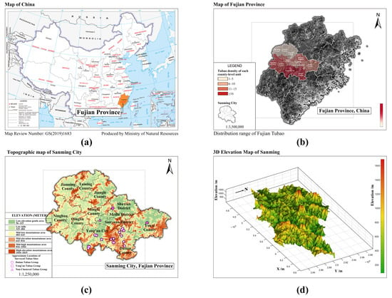
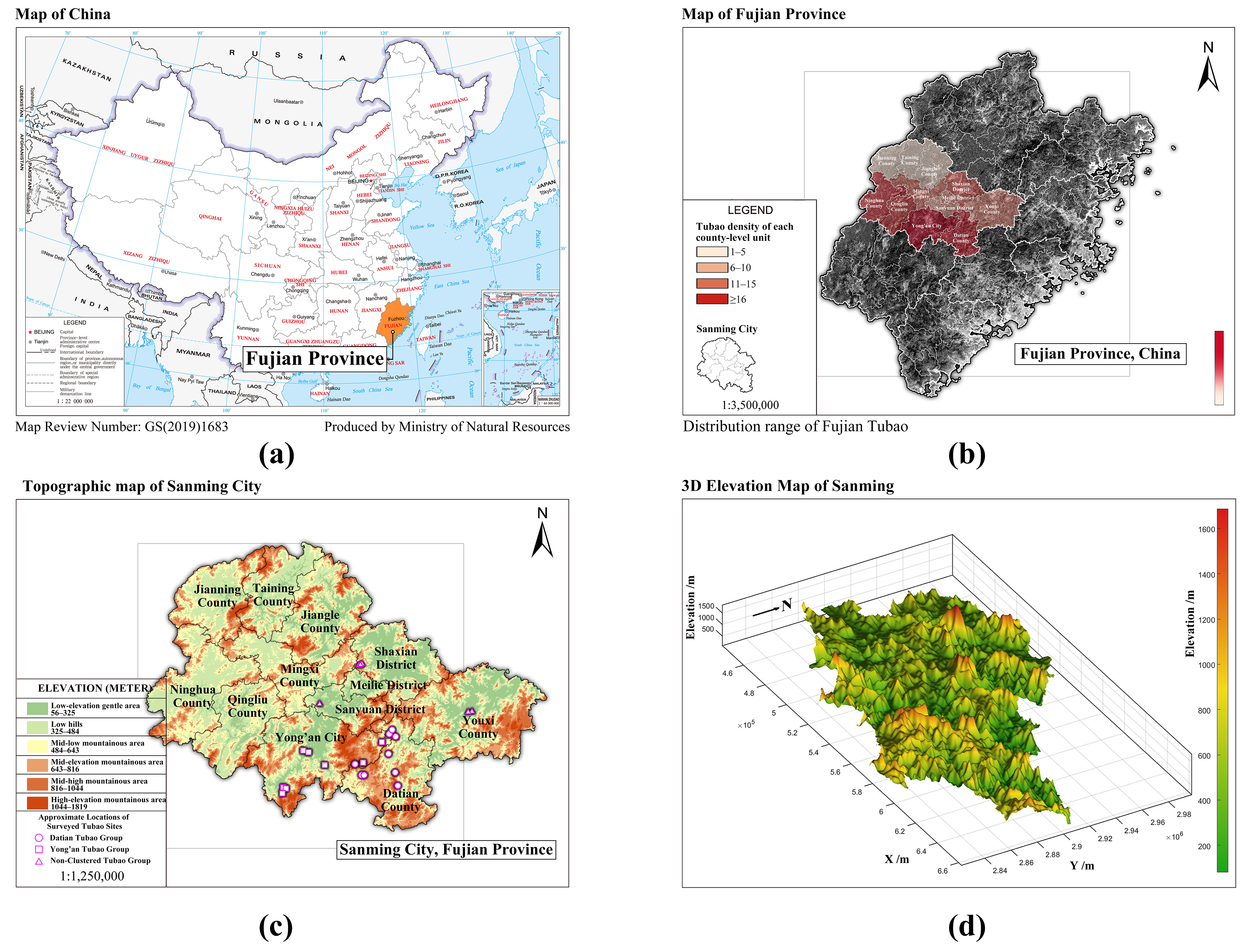
Central Fujian Tubao are concentrated in the mountainous and hilly areas of central Fujian, particularly in Sanming City and adjacent counties (Figure 1). Located between the Min and Jiulong river systems [29], the region comprises mountains, hills, valleys, and basins. Tubao typically consist of enclosed defensive walls built of stone masonry and rammed earth, inward-facing timber courtyards, and composite residential units. Quantifying Tubao colors can help document the visual characteristics of local materials and building traditions and provide preliminary conservation references. Their relatively consistent architectural forms and varied material surfaces support regional comparison within one heritage type.
Figure 1.
(a) Geographic location of Fujian Province in China; (b) distribution of Central Fujian Tubao; (c) topographic map of Sanming City; and (d) three-dimensional terrain map of Sanming City.
To examine color commonalities and regional variation within the same heritage type, the samples were divided into Datian-region, Yong’an-region, and non-clustered groups.
Sample selection favored relatively well-preserved Tubao that retained their architectural forms, spatial layouts, structural features, and surface-color information [30]. Priority was given to protected or listed sites, as well as unlisted examples that remained intact and representative of local characteristics. To maintain equal image counts for regional comparison, the target was set in advance at 12 images per group. A total of 36 images were selected from 24 Tubao, comprising 10 Datian-region, 8 Yong’an-region, and 6 non-clustered Tubao. Images were selected based on clear focus, suitable illumination, and nonredundant viewpoints, with priority given to coverage of different building-body materials and colors. Multiple images of the same Tubao were included to extend material and color coverage across different viewpoints. The correspondence between individual images and Tubao is provided in the “Image_building_mapping” sheet of Supplementary Material S2.
2.2. Methodology
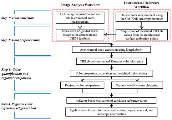
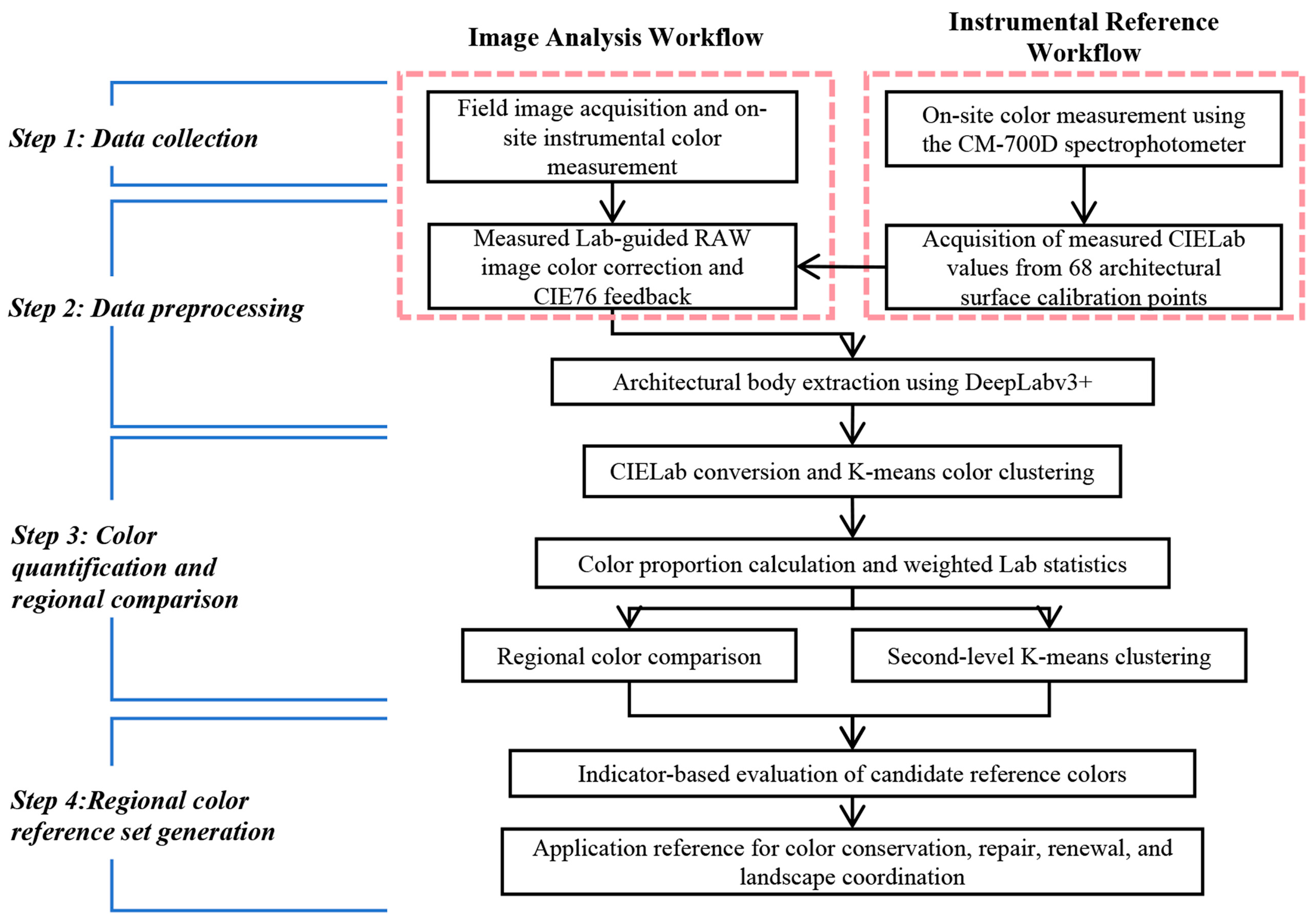
The methodology comprised four stages. First, field images and spectrophotometric CIELAB measurements were collected from Central Fujian Tubao. Second, RAW images were standardized in Adobe Camera Raw using the measured values as correction references, with ΔE*ab ≤ 6 adopted as the quality-control threshold. DeepLabv3+ was then used to extract the building-body regions. Third, two-level K-means clustering, pixel-area weighting, and statistical tests were applied to identify dominant colors, regional representative colors, and interregional differences. Finally, entropy-weighted TOPSIS ranked the candidate regional colors and classified them into core and auxiliary conservation reference palettes. The workflow is shown in Figure 2.
Figure 2.
C-D-K-based color quantification and entropy-weighted TOPSIS evaluation workflow.
2.2.1. Data Collection
Architectural photographs and spectrophotometric measurements were acquired concurrently. Images were captured with a Canon EOS 700D and EF-S 18–135 mm f/3.5–5.6 IS USM lens (Canon Inc., Tokyo, Japan), and colors were measured with a Konica Minolta CM-700D spectrophotometer (Konica Minolta, Inc., Osaka, Japan) using diffuse illumination/8° viewing geometry (de:8°) in specular component excluded (SCE) mode, with an 8 mm measurement aperture, CIE standard illuminant D65, and the CIE 1931 2° standard observer. Acquisition was conducted under stable daylight at 9:00–11:00 and 14:00–17:00, avoiding backlighting, direct sunlight, deep shadows, and highly reflective surroundings. The lens height, focal length, and aspect ratio were fixed at 1.61 m, 50 mm, and 3:2, respectively, to limit perspective and compositional variation [14].
Measurements covered representative rammed-earth, masonry, timber, roofing, and repaired or decorated surfaces. Highly reflective, stained, or severely damaged areas were excluded. Zero calibration was performed at the start of each morning and afternoon measurement session, and white calibration was performed after powering on the instrument at each Tubao. A single reading was obtained at each sampling point, and the resulting L*, a*, and b* values were recorded by region, Tubao, component, material, and surface condition [31]. Field acquisition relied on stable daylight, while sRGB-to-CIELAB conversion used the D65 reference white.
2.2.2. Data Preprocessing and Color Calibration
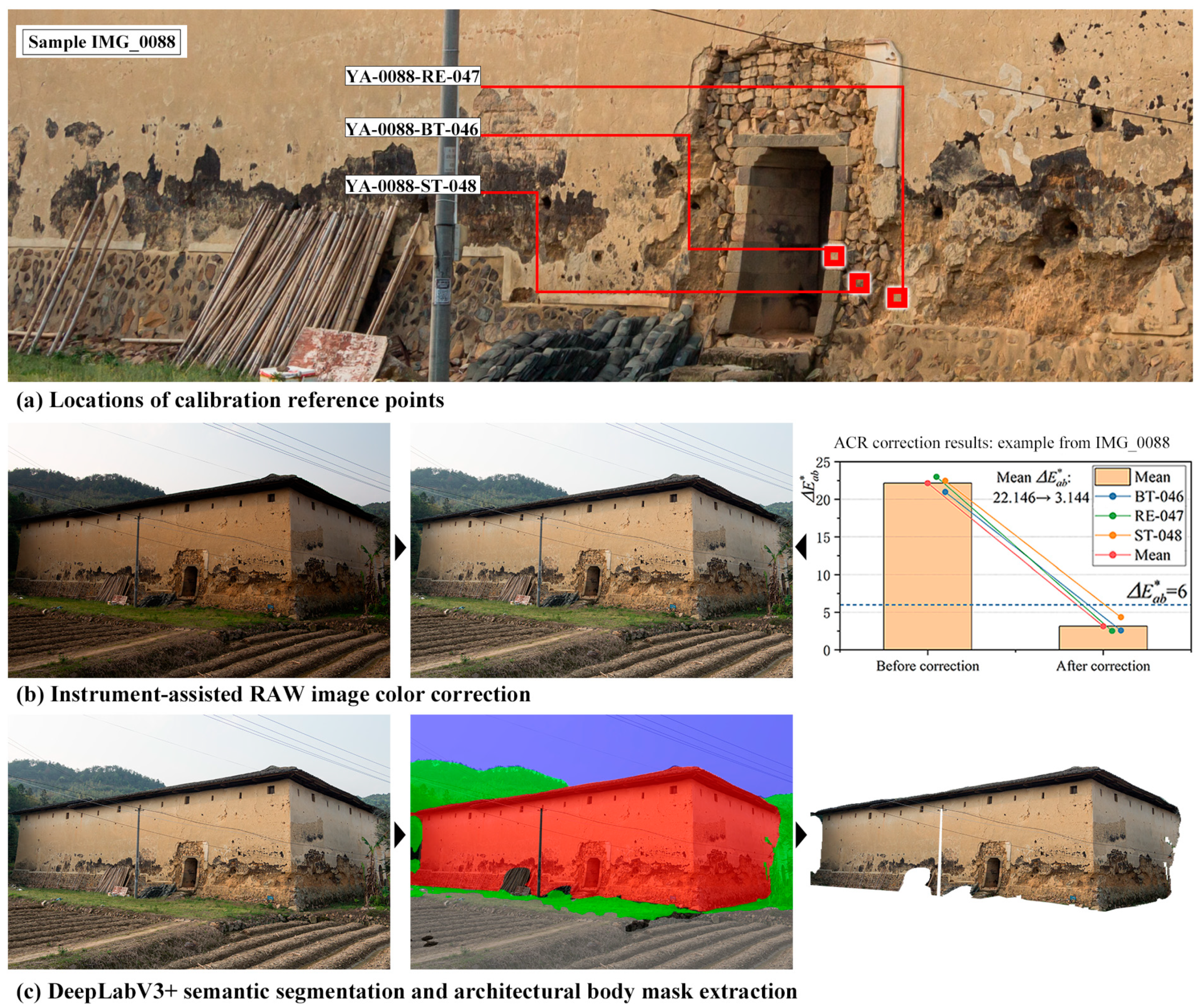
Field images are susceptible to variations in illumination, exposure, camera response, reflections, and shadows. To reduce these effects, 68 calibration reference points were established on the building surfaces and measured in CIELAB using the spectrophotometer. Corresponding image locations were identified manually using surface patterns in field measurement photographs and sampled using the mean color of a 12 × 12-pixel area in Adobe Photoshop on 3872 × 2581-pixel images. The fixed window size was a case-specific choice used to standardize sampling across images; its suitability for other cases and physical-area equivalence with the 8 mm instrument measurement aperture were not established. The original Canon RAW files (.CR2) were processed in Adobe Camera Raw 16.3.1 using a common starting preset (Process Version 15.4) to streamline processing, followed by image-specific manual adjustments to tonal, color, and optical correction settings as needed. The baseline settings included a custom white balance (5200 K; Tint +12), standardized tonal and color controls, chromatic-aberration removal, and lens-profile corrections for distortion and vignetting (both correction amounts set to 100). Field-measured CIELAB values guided the image-specific fine-tuning until the image-sampled colors approached the corresponding measurements. The baseline settings and final per-image ACR values recorded in the XMP sidecar files are provided in the “ACR_settings” worksheet of Supplementary Material S1. All 68 point pairs were used as calibration references. Color differences at these same locations were subsequently calculated to assess agreement with the calibration references. No separate holdout subset was used; therefore, these results describe calibration residuals rather than independent validation performance.
Color differences between the image and measured values were calculated using CIE76:
CIE76 expresses ΔE*ab as the Euclidean distance between two CIELAB coordinates [20]. It was used as a standardized and computationally straightforward measure of residual differences at the paired calibration points. To assess sensitivity to the choice of color-difference formula, CIEDE2000 (ΔE00) was additionally calculated before and after correction for the same 68 paired calibration points, with kL = kC = kH = 1 [32]. The two formulas were compared using descriptive statistics and the direction of change at each point. Detailed results are provided in the “DeltaE_comparison” sheet of Supplementary Material S1. A CIE76 threshold of ΔE*ab ≤ 6 was adopted as an operational upper limit for residual differences at the paired calibration points. This choice is consistent with the empirical interpretation used in soil-color measurement, in which differences of 3 ≤ ΔE*ab ≤ 6 are described as perceptible but acceptable [33]. Here, the criterion concerns agreement with the field-measured references at the sampled calibration locations; its suitability as a tolerance for restoration-material matching was not assessed. The 36 corrected images were used for subsequent analysis, with all 68 paired calibration points meeting this criterion.
DeepLabv3+ with a MobileNetV2 backbone and an output stride of 16 was fine-tuned for five-class segmentation of building bodies, sky, vegetation, ground, and miscellaneous objects using a Cityscapes-pretrained checkpoint [34]. The 36 manually annotated images used for color analysis were also used for model development. An image-level random split with a seed of 42 assigned 29 images to training and seven to internal validation. Images from four buildings occurred in both subsets; therefore, this split was used for internal model selection rather than independent building-level evaluation. Training used 512 × 512-pixel inputs, a batch size of four, and AdamW with an initial learning rate of 1 × 10⁻⁴ for 100 epochs. The checkpoint from epoch 64, which achieved the highest internal-validation IoU metric, was selected. Detailed settings and subset membership are provided in Supplementary Material S4.
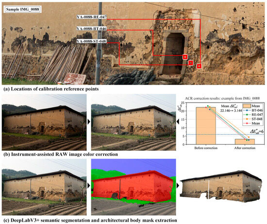
For color analysis, the predicted building-body masks were visually inspected and manually corrected by one author using Adobe Photoshop before K-means clustering. Corrections were guided by the corresponding original images: erroneously included non-building regions were removed, and omitted building regions were restored. This building-based inclusion rule was applied consistently across the 36 images. The final corrected masks were used to retain only building-body pixels for color clustering, reducing interference from non-building elements. Figure 3 illustrates the preprocessing and color calibration procedure. An example of manual refinement of a building-body mask is provided in Figure S1.
Figure 3.
Example workflow for image-data preparation and color calibration.
For the 36 development images, building-class IoU and Dice coefficients were calculated by comparing uncorrected model predictions with the original manual annotations at the original image resolution. Results were summarized separately for the training and internal-validation subsets. A supplementary segmentation assessment used six additional images, with two from each regional group. These images were excluded from model development and color analysis, although their buildings were represented in the development dataset. The fixed model’s uncorrected predictions were compared with manually annotated binary building masks using building-class intersection over union (IoU) and Dice coefficients. The reference masks were checked and refined after the initial evaluation to apply a consistent building-class definition; these revisions are documented in Supplementary Materials S4. Per-image metrics were summarized using the arithmetic mean and sample standard deviation.
2.2.3. Data Processing
Valid pixels were defined as pixels with alpha > 10, excluding those with R, G, and B all ≥245 (0–255 scale). Building-body pixels were clustered in the CIELAB color space using K-means [35]. For each image, the cluster centers and their pixel-area proportions relative to the total number of valid pixels were recorded. These proportions were used as weights to calculate image- and regional-level weighted CIELAB indicators. After all valid pixels were assigned to clusters, each reported CIELAB center was recalculated as the arithmetic mean of the valid pixels within that cluster. The image-level indicators were calculated by weighting these centers by their corresponding pixel proportions, as expressed below. This weighted sum equals the mean CIELAB coordinates of all valid pixels included in the analysis. These indicators summarize average lightness and color tendency rather than palette structure. Cluster centers and their proportions were retained separately for descriptive comparisons of representative-color combinations and their relative proportions.
where X denotes one of the CIELAB coordinates L, a, or b, and X*w denotes the corresponding image-level weighted indicator. K = 6 is the number of first-level clusters, Cj is the set of valid pixels assigned to cluster j, and is their arithmetic mean for coordinate X. nj is the number of valid pixels in cluster j, N is the total number of valid pixels in the image, and pj = nj/N is the corresponding pixel proportion. X*i is the coordinate value of valid pixel i.
The K-means procedure comprised four steps:
- (a).
- Initialization: Select k initial color-cluster centers, μi (1 ≤ i ≤ k), from the image data.
- (b).
- Assignment: Calculate the Euclidean distance between each color data point and each cluster center μi, and assign the data point to the cluster Ci associated with the nearest cluster center.
- (c).
- Update: Calculate the mean of all color data points within cluster Ci and use it as the new cluster center μi for the next iteration.
- (d).
- Convergence: Repeat steps (b) and (c) until the changes in the cluster centers become negligible or the predefined maximum number of iterations is reached [36].
The Euclidean distance was calculated using Equation (3).
where x denotes a color point, Ci denotes the ith cluster, μi denotes its cluster center, and m = 3 corresponds to the three CIELAB dimensions L*, a*, and b*. The terms xj and μij denote the values of x and μi in the jth dimension, respectively.
K-means was implemented using scikit-learn with k-means++ initialization, a random seed of 42, and a maximum of 500 iterations. Twenty initializations were used at the image level and 50 at the regional level. Each image contributed up to 200,000 valid pixels sampled without replacement for fitting. Second-level K-means used the within-image pixel-area proportions of first-level clusters as sample weights. These weights summed to 1 per image, giving each selected image equal total weight. Regional color proportions were calculated by dividing each regional cluster’s summed weight by 12, the number of images per region.
K = 6 was retained at both clustering stages to provide a common six-color resolution for palette comparison. Following established cluster-validity methods [37,38], supplementary analyses examined K = 1–15 at both stages. Image-level compactness was assessed using RMSSTD (root mean square standard deviation) and its decrease from the preceding K, calculated on a fixed pixel sample for each image. RMSSTD was calculated using Equation (4).
where k denotes the number of clusters, Ci the ith cluster, μi its fitted center, x a sampled color point assigned to Ci, and N the number of sampled color points used for fitting. The term d(x, μi) denotes the Euclidean distance between x and μi, while m represents the data dimensionality. Because clustering was performed using the CIELAB coordinates L*, a*, and b*, m = 3. A lower RMSSTD indicates greater within-cluster compactness. Since RMSSTD generally decreases as k increases, its trend and adjacent-K decreases were used to assess diminishing improvements in compactness.
Regional compactness was assessed using the weighted sum of squared errors (SSE), with image-level K fixed at 6. All nine combinations of image-level and regional K in {5,6,7} were compared with the (6,6) reference using Earth Mover’s Distance (EMD), based on color proportions and CIE76 distances [39]. Detailed methods and results are provided in Supplementary Material S5 and Figures S2 and S3.
2.2.4. Indicator-Based Evaluation of Candidate Regional Reference Colors
The six regional representative colors generated for each Tubao group through second-level K-means clustering were treated as candidate regional reference colors. The 216 first-level dominant colors were used only to calculate the evaluation indicators.
Five indicators were included: regional representativeness, sample support, within-cluster stability, regional centrality, and chroma moderation. These were quantified using candidate-color area proportion, the number of assigned first-level colors, the weighted mean color difference from assigned colors, the color difference from the regional weighted CIELAB center, and the absolute deviation of C*ab from the regional weighted median C*ab, respectively. Within-image pixel-area proportions were used as weights for both the mean color difference to assigned colors and the regional median C*ab; the latter was calculated from all 72 first-level colors in each region. Regional representativeness and sample support were benefit indicators, whereas the remaining three were cost indicators. Proportion and member count reflect color coverage and support from first-level clusters, respectively, with potential overlap. Chroma moderation favors colors near the observed regional median as a preference for preliminary color coordination rather than a criterion for historical authenticity.
Entropy-weighted TOPSIS (Technique for Order Preference by Similarity to an Ideal Solution) was used to rank the candidate colors [40,41,42]. After directional transformation and min–max normalization, entropy weights were calculated from the variation in each indicator. TOPSIS then determined the distances of each candidate from the positive and negative ideal solutions and calculated its relative closeness coefficient, CCi, using Equations (5) and (6).
where ej denotes the information entropy of the jth indicator, pij the normalized proportion of the ith candidate color under that indicator, and n the number of candidate colors. The terms dj and wj denote the difference coefficient and entropy weight, respectively, while m = 5 represents the five evaluation indicators. Σl=1mdl is the sum of the difference coefficients across all indicators. Di+ and Di− denote the distances of candidate i from the positive and negative ideal solutions, while zij denotes the normalized indicator value and zj+ and zj− are the maximum and minimum of wjzij across the 18 candidates, respectively. CCi is the relative closeness coefficient, with a larger value indicating a better-performing candidate. Candidates were ranked by CCi within each region; the top three were classified as core reference colors and the remainder as auxiliary reference colors. Sensitivity analyses compared equal weighting, omission of proportion or member count, and selection of two to four core colors using Spearman rank correlations and core-color membership (Supplementary Material S3).
3. Results
3.1. Sample Collection Results for the Study Area
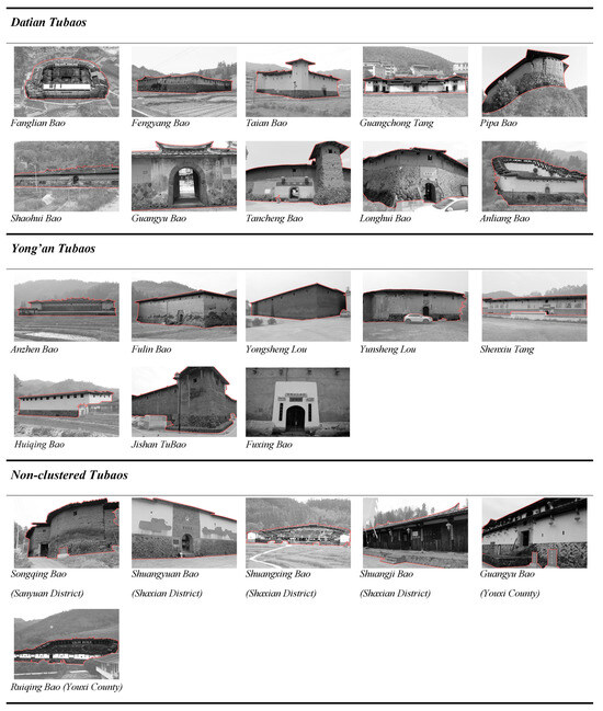
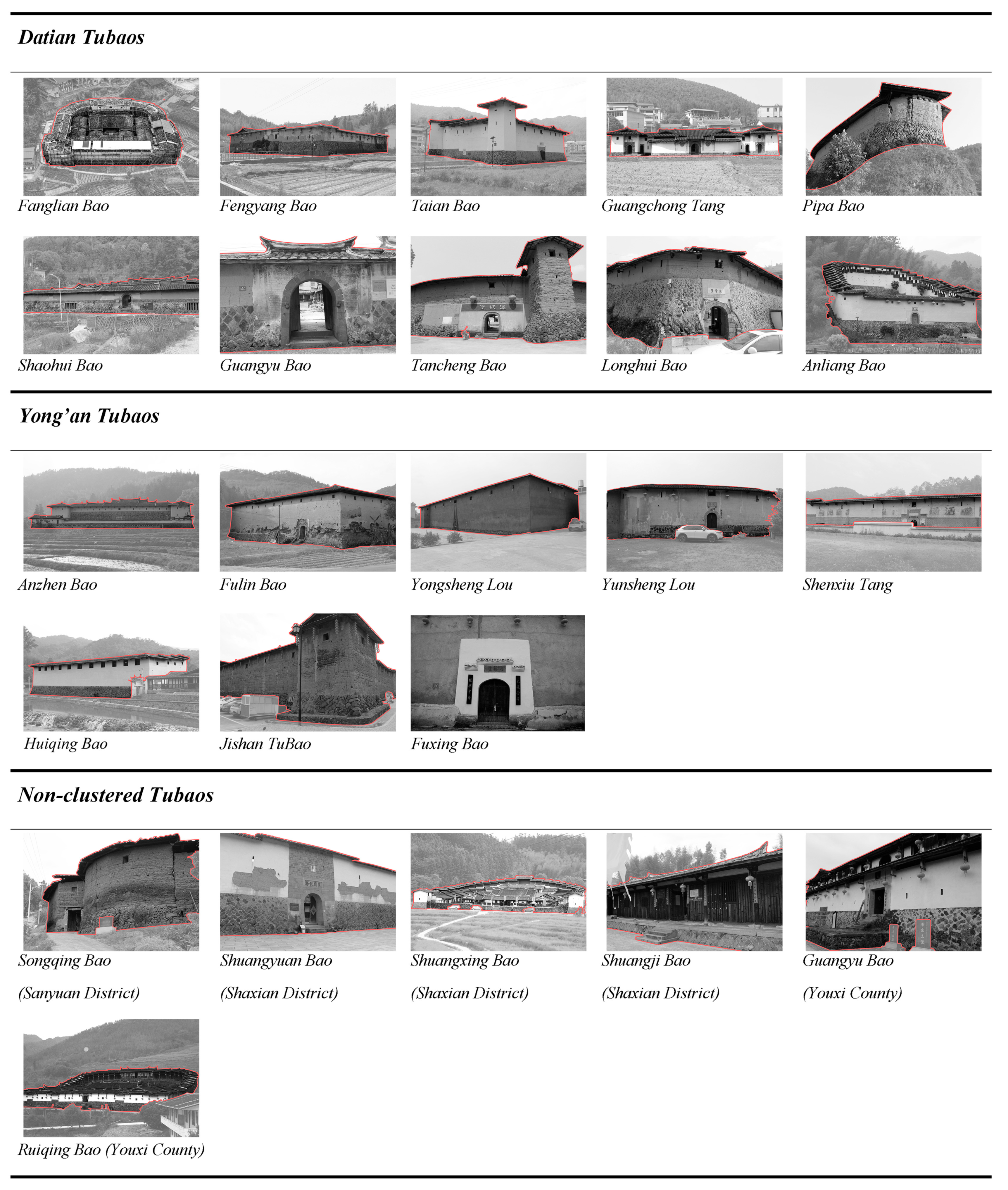
To support regional comparisons, the study considered differences among the Tubao in their siting environments, architectural forms, and preservation conditions [43,44,45] when selecting the specific research samples. The sample sources and data composition are presented in Table 1, and representative views of the 24 sampled Tubao are shown in Figure 4.
Table 1.
Sample Sources and Data Composition of Central Fujian Tubao.
Figure 4.
The 24 sampled Tubao in central Fujian.
3.2. Results of Image Color Calibration and Building-Body Segmentation
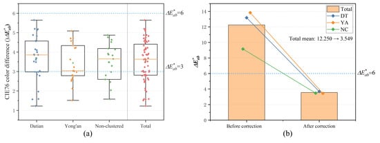
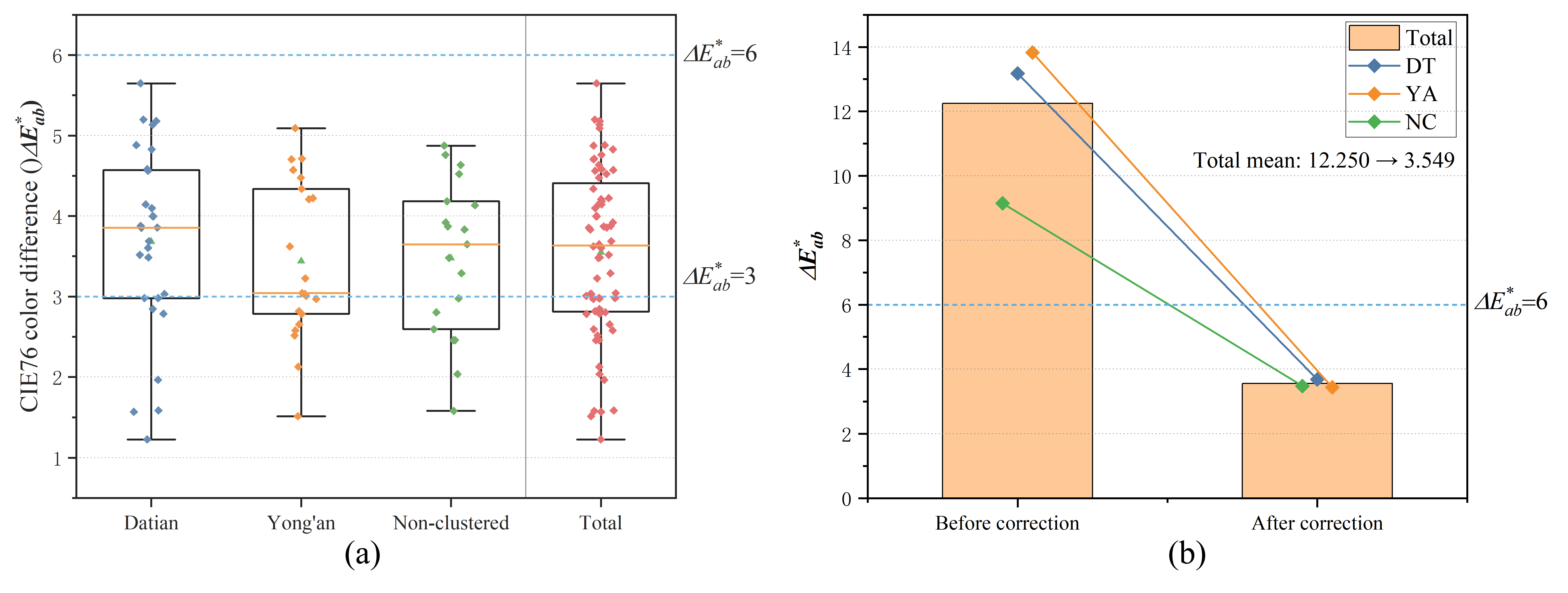
Color differences before and after image calibration were summarized for the 68 calibration point pairs, with complete point-by-point data provided in Supplementary Material S1. Before correction, the mean ΔE*ab was 12.250 ± 7.028, with a median of 10.387 and a range of 3.123–33.326. After correction, the mean decreased to 3.549 ± 1.048, with a median of 3.635 and a range of 1.227–5.648, and all residuals at the calibration points met the predefined quality-control threshold. For CIEDE2000, the mean ΔE00 decreased from 9.902 ± 6.124 before correction to 3.063 ± 1.125 after correction. The two formulas agreed on the direction of change at 66 of the 68 calibration points. These results indicate improved agreement between image-derived colors and the field-measured references at the calibration points. They do not establish color accuracy at other locations within the selected images that were not paired with field measurements. Figure 5 presents the comparison before and after correction and the distribution of the corrected values.
Figure 5.
(a) Distribution of corrected ΔE*ab by Tubao region (orange horizontal lines indicate medians); (b) ΔE*ab before and after ACR correction.
For the 36 development images, the mean building-class IoU was 0.9621 ± 0.0304 for the training subset (n = 29) and 0.9225 ± 0.0497 for the internal-validation subset (n = 7). The corresponding Dice coefficients were 0.9805 ± 0.0161 and 0.9591 ± 0.0272, respectively. These metrics compare uncorrected model predictions with the original manual annotations. The internal-validation subset was used for model selection and therefore does not constitute an independent test. Detailed results are provided in the “Development_results” sheet of Supplementary Material S4.
For the six supplementary test images, the mean building-class IoU was 0.9299 ± 0.0369, ranging from 0.8840 to 0.9710. The mean Dice coefficient was 0.9634 ± 0.0198, ranging from 0.9384 to 0.9853. Values are reported as mean ± sample standard deviation across images. Per-image results and pixel counts are provided in the “Segmentation_results” sheet of Supplementary Material S4. These results describe agreement between uncorrected model predictions and the final manual reference masks for additional views of buildings represented in the development dataset. They do not establish image-color accuracy or segmentation performance on previously unseen buildings.
3.3. Analysis of Clustering Results
The overall mean image-level RMSSTD was 4.336, 4.001, and 3.749 at K = 5, 6, and 7, respectively, showing diminishing improvements in compactness. Regional weighted SSE also decreased as K increased (Figure S2). The curves did not establish K = 6 as a unique optimum. Across the nine tested configurations, regional palettes retained broadly muted brown–gray tones, while individual centers and proportions changed (Figure S3). EMD relative to the (6,6) reference ranged from 1.776 to 6.438 across regions and the eight alternative configurations (Supplementary Material S5).
3.3.1. Regional Differences in Building-Level CIELAB Indicators Based on First-Level Clustering
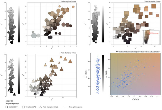
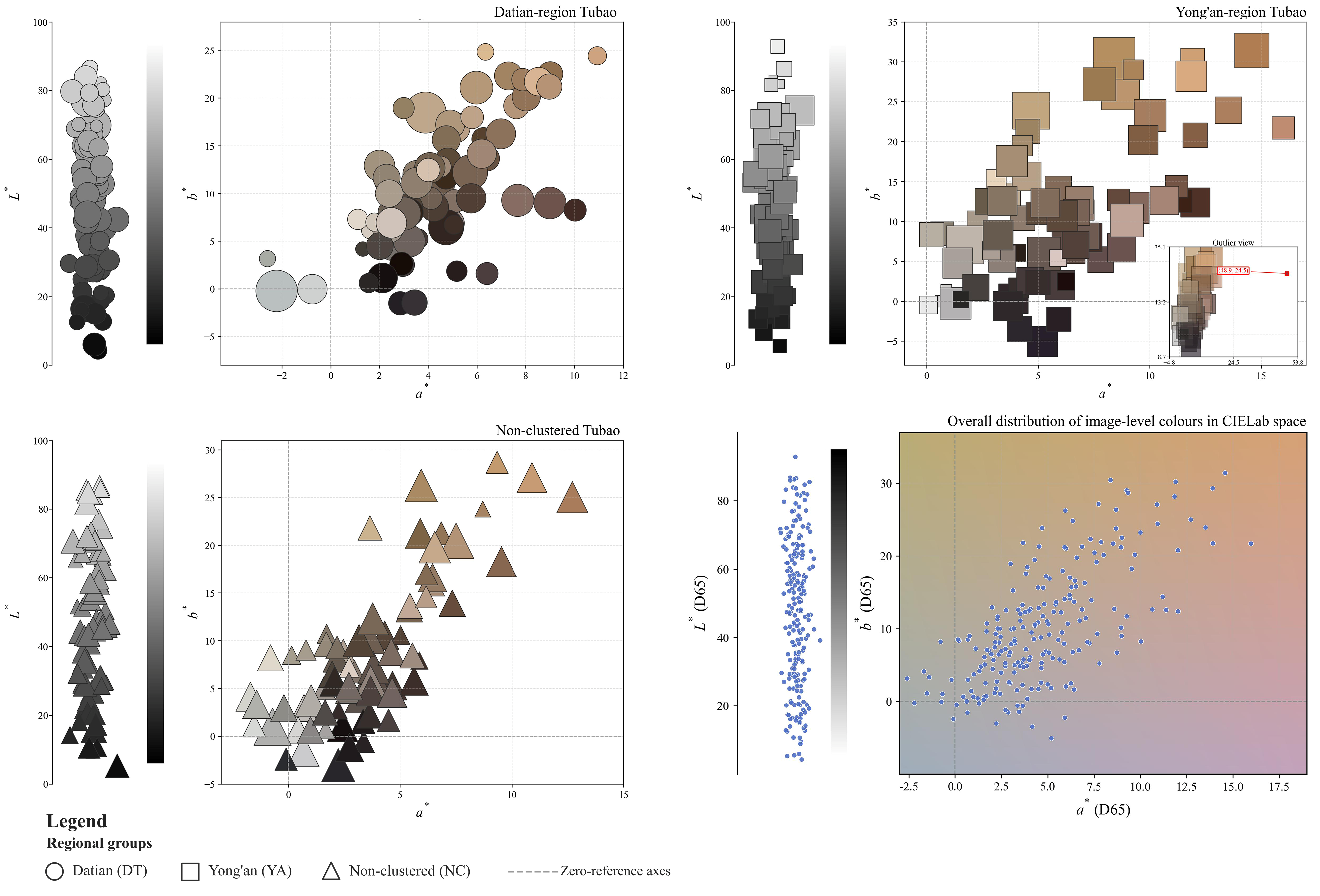
Based on the 216 dominant colors obtained through first-level K-means clustering, their distributions were first projected onto the CIELAB a*–b* plane and visualized using bubble plots for the three Tubao groups. Bubble size represents the pixel-area proportion of the corresponding dominant color relative to the total number of valid pixels in each image, thereby showing both its color direction and area weight. The regional bubble plots and the overall scatter distribution are presented in Figure 6. The 216 first-level dominant colors were then aggregated into 36 sets of image-level weighted CIELAB indicators, representing the mean CIELAB coordinates of the valid pixels in each image. To avoid treating multiple images of the same Tubao as separate observations in regional comparisons, each building-level indicator was calculated as the arithmetic mean of the corresponding image-level values across all selected images of that Tubao. This yielded 24 building-level observations: 10 Datian-region, 8 Yong’an-region, and 6 non-clustered Tubao. Each Tubao contributed one observation with equal weight to the regional comparisons. These building-level summaries represent the selected views and should not be interpreted as surface-area-weighted color averages of entire buildings.
Figure 6.
Distribution of image-level dominant colors for the three Tubao groups in the CIELAB a*–b* plane (bubble colors represent the extracted colors, bubble sizes are proportional to their corresponding color proportions).
Before the group comparisons, the Shapiro–Wilk and median-centered Levene tests were used to assess normality within each regional group and homogeneity of variance, respectively, using the building-level indicators [46]. All assumption tests yielded p > 0.05, and regional differences in L*w, a*w, and b*w were therefore assessed using one-way analysis of variance, with each Tubao contributing one observation. Statistical significance was defined as p < 0.05. No post hoc pairwise comparisons were performed because none of the three omnibus tests was statistically significant. The regional comparison results are presented in Table 2, while the detailed first-level clustering results, image-level weighted CIELAB indicators, building-level summaries, and results of the assumption tests and omnibus tests are provided in Supplementary Material S2.
Table 2.
Descriptive Statistics and Regional Difference Tests for Building-Level CIELAB Indicators.
As shown in Figure 6, the first-level dominant colors of the three regions were concentrated primarily in the a* > 0 and b* > 0 portions of the CIELAB plane. The three groups also overlapped substantially in the a*–b* plane, indicating a degree of commonality in their dominant-color distributions. The building-level comparisons in Table 2 did not detect statistically significant regional differences in L*w (F = 0.055, p = 0.947), a*w (F = 2.781, p = 0.085), or b*w (F = 0.854, p = 0.440). These nonsignificant results do not establish equivalence among the three regional groups.
3.3.2. Construction of Regional Representative Palettes Based on Second-Level K-Means Clustering
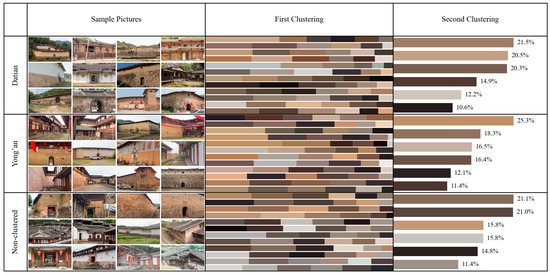
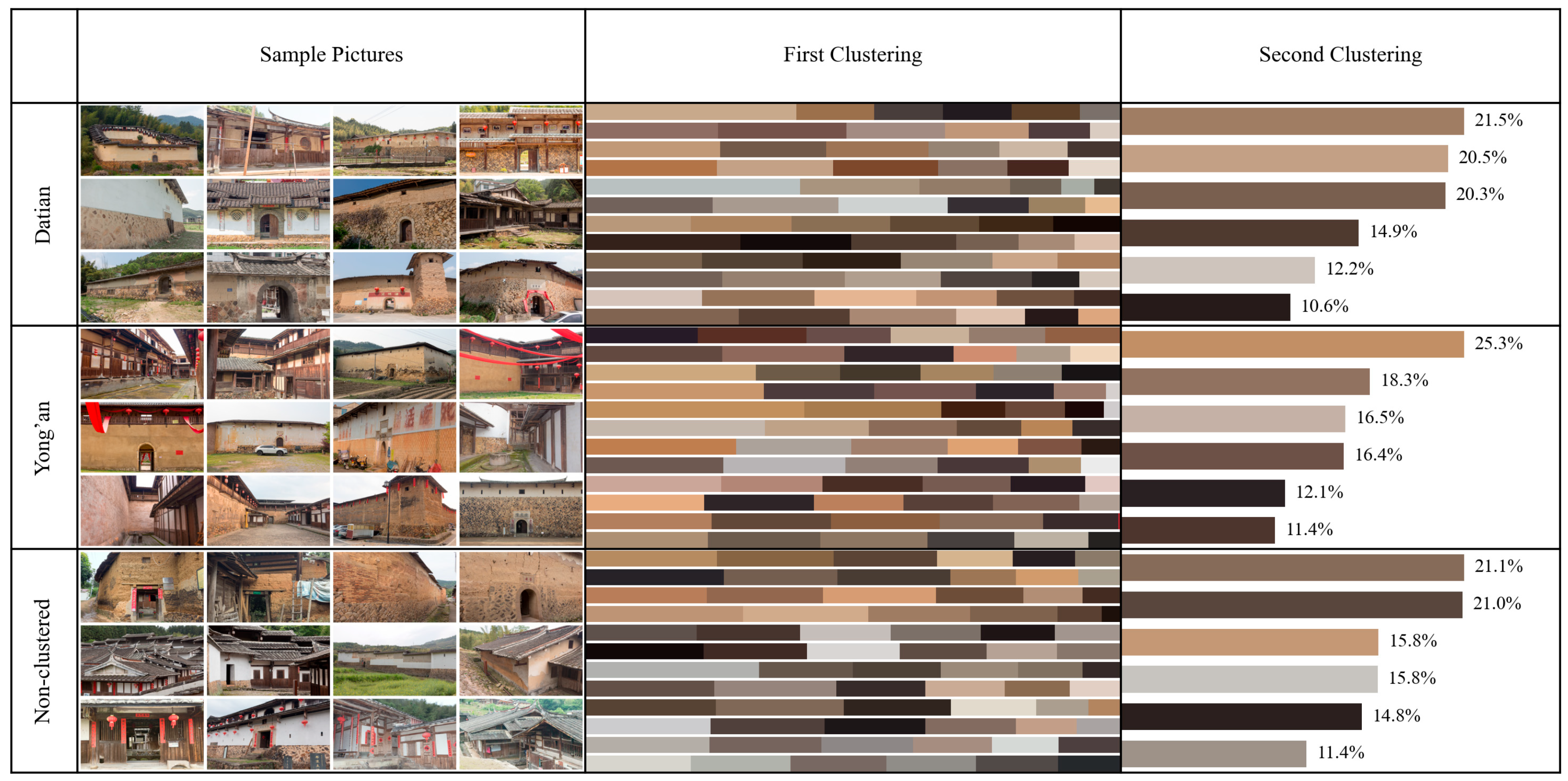
Using the dominant colors obtained through first-level K-means clustering, the 72 first-level dominant colors from each of the Datian-region, Yong’an-region, and non-clustered Tubao groups were separately subjected to second-level K-means clustering. Six regional representative colors were extracted for each group, forming three regional representative palettes. Figure 7 illustrates the progression from the sample images of the three Tubao groups through the first-level clustering results to the second-level regional representative palettes.
Figure 7.
Second-level K-means clustering results for the regional representative color palettes of the three Tubao groups.
3.4. Generation of Conservation Reference Palettes Through Indicator-Based Evaluation
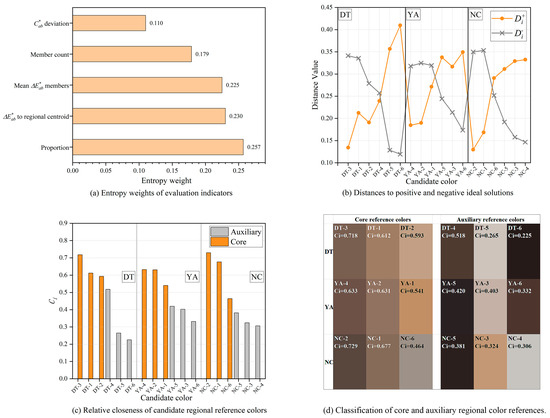
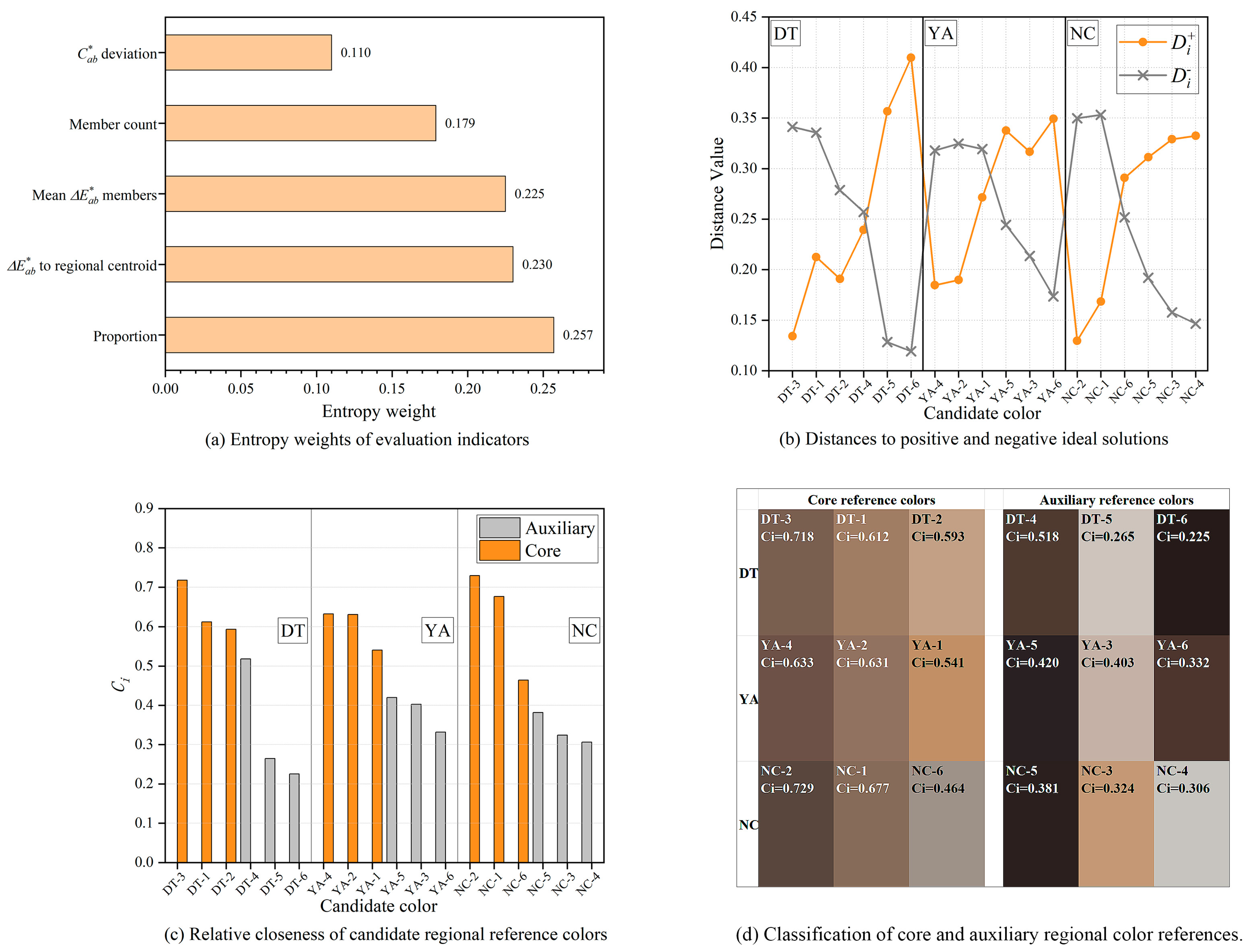
The 18 regional representative colors obtained through second-level K-means clustering were treated as candidate regional reference colors and comprehensively evaluated using entropy-weighted TOPSIS. The complete normalized matrix, entropy weights, and TOPSIS calculations are provided in Supplementary Material S3, while the main results are presented in Figure 8. The entropy-weighting results assigned weights of 0.257 to regional proportion, 0.230 to regional centrality, 0.225 to within-cluster stability, 0.179 to the number of assigned first-level dominant colors, and 0.110 to chroma moderation, as shown in Figure 8a. TOPSIS was then used to calculate the distances of each candidate color from the positive and negative ideal solutions, Di+ and Di−, respectively, as presented in Figure 8b. Based on these distances, the candidate colors were ranked within each region according to their relative closeness coefficients, CCi, as shown in Figure 8c. The three highest-ranked candidates were DT-3, DT-1, and DT-2 for Datian; YA-4, YA-2, and YA-1 for Yong’an; and NC-2, NC-1, and NC-6 for the non-clustered group. These colors were classified as core reference colors, while the remaining candidates were classified as auxiliary reference colors. The resulting classification of core and auxiliary regional reference colors is presented in Figure 8d. Equal weighting retained all sets of core colors (Spearman ρ = 1.000 for DT and 0.943 for YA and NC). However, omitting proportion changed one core color in each of DT and YA, and selecting four core colors yielded different YA sets under entropy and equal weighting (Supplementary Material S3).
Figure 8.
Entropy-weighted TOPSIS evaluation and classification of candidate regional reference colors. (a) Entropy weights of the five evaluation indicators; (b) distances of candidate colors to the positive and negative ideal solutions; (c) TOPSIS closeness coefficients; (d) core and auxiliary regional reference colors ranked by TOPSIS score.
4. Discussion
4.1. Color Commonalities and Differences in Palette Structure
The first-level clustering results showed that the dominant colors of the three Tubao groups were concentrated primarily in the a* > 0 and b* > 0 regions, indicating an overall tendency toward warm reddish-brown and yellowish-brown tones in the building bodies. Regional comparisons using the building-level summaries did not detect statistically significant differences among Datian-region, Yong’an-region, and non-clustered Tubao in L*w, a*w, or b*w. The descriptive results further showed that Yong’an-region Tubao had the highest mean a*w in the present sample, indicating a more pronounced positive shift along the red–green axis. This descriptive pattern does not establish a statistically significant regional difference.
The second-level clustering results provided a descriptive comparison of the selected regional image sets. Although the three Tubao groups shared basic tones such as grayish brown, yellowish brown, dark brown, and low-lightness neutrals, their representative-color combinations and proportional structures were not identical. Datian-region Tubao showed relatively balanced color-block proportions and more continuous transitions among light yellowish brown, grayish brown, and medium-lightness earth tones. Reddish-brown and dark-brown blocks were more prominent in Yong’an-region Tubao, consistent with their descriptively higher building-level mean a*w. Non-clustered Tubao, by comparison, exhibited a clearer tendency toward grayish-brown tones and a greater concentration of darker colors. These findings describe a shared range of basic tones together with variation in representative-color combinations and color-block proportions in the selected images. These palette comparisons are descriptive; regional differences in palette structure were not statistically tested. Regional palettes were generated by assigning equal total weight to each selected image. As some Tubao were represented by more images than others, their contributions to the regional palettes were unequal. The palettes should therefore be interpreted as descriptive summaries of the selected image sets and may be more strongly influenced by buildings represented by multiple views. The coexistence of these commonalities and differences may be associated with their similar material foundations, including rammed-earth walls, stone bases, timber components, and tiled roofs, as well as variations in weathering, restoration, and component proportions among individual buildings.
4.2. Improving the Reliability of Image Color Data Within the C-D-K Framework
Unlike previous studies that relied primarily on a single image source, such as street-view imagery or high-resolution photography [14,15], this study established a paired correction procedure linking spectrophotometric measurements with colors sampled from corresponding image locations. Specifically, field-measured CIELAB values from 68 calibration reference points on building surfaces were used as references to adjust white balance, exposure, contrast, and basic color parameters during RAW image preprocessing, progressively bringing the image-sampled colors closer to the field measurements. After correction, all 68 paired calibration points satisfied the operational CIE76 criterion of ΔE*ab ≤ 6. Both CIE76 and CIEDE2000 showed lower mean residual color differences after correction, and the two formulas agreed on the direction of change at 66 of the 68 points. Thus, the aggregate finding of reduced calibration residuals was consistent across the two formulas, although their point-specific assessments were not identical. These findings concern agreement at the calibration locations; color accuracy beyond these locations remains untested. In addition to dominant-color extraction and descriptive interpretation after K-means clustering [47], this study further applied assumption checks and one-way analysis of variance to assess regional differences in the building-level CIELAB indicators.
The core of the C-D-K framework therefore lies in transforming environmentally affected images into analyzable data constrained by field measurements. The measured values were used to guide image color calibration, with ΔE*ab providing feedback on the differences between image-sampled colors and field-measured references at the paired locations. The corrected images were subsequently used for DeepLabv3+ segmentation, K-means clustering, and regional statistical analyses. Finally, cluster centers, pixel-area proportions, and regional distributions were integrated to generate data-driven conservation reference palettes, providing a reusable method for color conservation in vernacular built heritage. The framework can be adapted in practice to different heritage types and data-acquisition conditions.
4.3. Application of Data-Driven Conservation Reference Palettes
The regional representative colors generated through second-level K-means clustering were not directly treated as the final conservation reference palettes [15]. Instead, entropy-weighted TOPSIS was used to conduct a multi-indicator evaluation of the candidate colors. This approach avoids the limitations of selecting colors solely according to area proportion and allows the final reference colors to account simultaneously for regional representativeness, support from first-level dominant colors, within-cluster stability, regional centrality, and chroma moderation. The results showed that the core reference colors did not necessarily correspond to those with the largest area proportions but were the candidates closest to the ideal reference colors under the combined influence of multiple indicators. Selecting three core colors is an operational choice for organizing the reference palettes, with membership dependent on indicator selection.
The core reference colors of the DT, YA, and NC groups were dominated by low- to medium-chroma grayish-brown, earthy-yellow, and reddish-brown tones, indicating that Central Fujian Tubao share relatively consistent overall color characteristics shaped by their building materials, construction methods, and long-term weathering. However, the combinations and ordering of core and auxiliary colors differed across regions. The regional reference palettes should therefore not be merged into a single universal color chart but should instead be expressed through a shared color framework combined with region-specific reference color sets.
The palettes describe current observed appearance and provide preliminary references for comparing material samples. Restoration use requires component identification, material analysis, historical and intervention records, on-site verification, and independent assessment of color accuracy.
4.4. Method Applicability, Boundary Conditions, and Limitations
The C-D-K color-quantification framework developed in this study is applicable to research on vernacular built heritage that focuses on the exterior colors of building bodies and requires regional comparison and conservation-palette generation. Although the framework can reduce the effects of background interference and acquisition errors on dominant-color extraction, it is more suitable for regional architectural heritage characterized by similar architectural forms, materials, and construction logic. When the study objects differ substantially in architectural type, scale, or material system, the comparability of the color results and the robustness of their interpretation may decrease. Future studies could independently test the framework on other vernacular building types, adapting image acquisition, segmentation, color calibration, and evaluation criteria to each case.
The samples examined in this study were concentrated on representative Central Fujian Tubao and therefore cannot fully capture variations associated with different construction periods, preservation conditions, and restoration stages. The regional statistical comparisons were based on 24 purposively selected Tubao, and the small samples within each regional group may limit the ability to detect regional differences and generalize the findings beyond the studied buildings. Because the building-level summaries were derived from selected views, they may not fully capture the color composition of entire buildings. Image colors may still be affected by natural lighting, shadows, reflections, surface staining, weathering, and camera imaging mechanisms. All 68 point pairs were used for calibration, leaving no independent set for evaluating color accuracy beyond the calibration points. Future studies should assess corrected image colors using measurement–image point pairs withheld from the calibration process. The supplementary segmentation assessment was limited to six additional views of buildings represented in the development dataset, and the reference masks were refined after the initial evaluation. Future assessments should hold out entire buildings and finalize reference annotations before examining model predictions. The K-means results are also influenced by the number of clusters, initial cluster centers, segmentation accuracy, and pixel weighting. Moreover, the entropy-weighted TOPSIS results depend on the indicator system, normalization method, and candidate-color set defined in this study. The relative closeness coefficient, CCi, represents only the relative ranking of candidate colors within the present evaluation system rather than an absolute criterion for applicability. The palettes pool colors from different materials and components without distinguishing original surfaces from later interventions. Their historical authenticity remains unverified. Future studies could improve the stability and practical adaptability of the color reference sets by expanding the sample, collecting images across multiple periods, increasing the number of field measurement points, and incorporating material analysis and on-site sample comparisons.
5. Conclusions
This study addressed how color data extracted from images of vernacular built heritage can be transformed into conservation reference palettes. A C-D-K color-quantification framework integrating CIE76-guided image color calibration, DeepLabv3+ building-body segmentation, and K-means color clustering, followed by entropy-weighted TOPSIS evaluation, was developed and applied using Central Fujian Tubao as a case study. The main conclusions are as follows.
- (1)
- A color-data processing pathway comprising field-guided image color calibration, building-body extraction, clustering analysis, and comprehensive evaluation was established. Image colors were corrected using feedback from spectrophotometrically measured Lab values, reducing the mean residual color differences calculated using CIE76 and CIEDE2000 across the 68 calibration point pairs. DeepLabv3+ building-body mask extraction further reduced interference from background elements such as the sky, vegetation, and ground.
- (2)
- Application of the framework showed that the three Tubao groups shared low- to medium-chroma basic tones, including warm grayish brown, earthy yellow, and reddish brown, while the extracted palettes showed descriptive variation in representative-color combinations, light–dark hierarchies, and proportional structures across the selected regional image sets. Building-level comparisons did not detect statistically significant regional differences in L*w, a*w, or b*w. These findings provide a descriptive basis for considering both shared basic tones and variation in palette composition when developing conservation reference palettes.
- (3)
- The regional representative colors generated through second-level K-means clustering were treated as candidate regional reference colors and ranked and classified using entropy-weighted TOPSIS, producing core and auxiliary reference palettes. The resulting palettes describe current observed appearance and provide preliminary color references. Restoration use requires independent assessment of color accuracy and verification against material, component, historical, and on-site evidence.
Supplementary Materials
The following supporting information can be downloaded at https://www.mdpi.com/article/10.3390/buildings16214245/s1: Supplementary Material S1: S1_Measured-Image_CIE76V3.1.xlsx; Supplementary Material S2: S2_Tubao_Kmeans_results_V5.1.xlsx; Supplementary Material S3: S3_Tubao_entropy_TOPSIS_V2.xlsx; Supplementary Material S4: S4_DeepLab_training_and_segmentation_results_V4.xlsx; Supplementary Material S5: S5_Kmeans_validity_and_sensitivity_V1.xlsx; Supplementary Figure S1: Figure_S1_Manual_mask_refinement.pdf; Supplementary Figure S2: Figure_S2_Kmeans_validity.pdf; Supplementary Figure S3: Figure_S3_Kmeans_palette_sensitivity.pdf.
Author Contributions
Z.Q.: Conceptualization; Data curation; Methodology; Investigation; Software; Validation; Writing—original draft; Project administration. L.Z.: Investigation; Data curation; Writing—original draft. X.L.: Resources; Writing—review and editing; Supervision; Formal analysis. Z.C.: Writing—review and editing; Funding acquisition; Supervision; Resources. All authors have read and agreed to the published version of the manuscript.
Funding
This work was supported by the Industry–University Cooperation Project in the Field of Social Development of the Fujian Provincial Department of Science and Technology, “Construction and Application of a Color Map of Traditional Dwellings in the Minjiang River Basin Based on Indigenous Residents’ Color Preferences” (Grant No. 2023Y4003).
Data Availability Statement
Data supporting the reported analyses are provided in Supplementary Materials S1–S5. Additional data are available from the corresponding author upon reasonable request.
Acknowledgments
The authors thank the local heritage administrators and residents who facilitated site access and field data collection.
Conflicts of Interest
The authors declare no conflicts of interest.
Abbreviations
The following abbreviations are used in this manuscript:
| ICOMOS | International Council on Monuments and Sites |
| DT | Datian-region Tubao |
| YA | Yong’an-region Tubao |
| NC | Non-clustered Tubao |
| C-D-K | CIE76–DeepLabv3+–K-means workflow |
| GIS | Geographic information system |
| ACR | Adobe Camera Raw |
| CIE | International Commission on Illumination |
| CIELAB | CIE 1976 L*a*b* color space |
| CIE76 | CIE 1976 L*a*b* color-difference formula |
| CIEDE2000 | CIE 2000 color-difference formula |
| HSV | Hue, saturation, and value |
| sRGB | Standard RGB color space |
| SCE | Specular component excluded |
| FCN | Fully convolutional network |
| AdamW | Adam with decoupled weight decay |
| IoU | Intersection over union |
| RMSSTD | Root mean square standard deviation |
| SSE | Sum of squared errors |
| EMD | Earth Mover’s Distance |
| ANOVA | Analysis of variance |
| TOPSIS | Technique for Order Preference by Similarity to an Ideal Solution |
| CCi | Relative closeness coefficient of candidate i |
References
- Cheshmehzangi, A. Urban Regeneration and Building Colours: Mapping Visual and Perceptual Dimensions of Dali’s Old Towns. In Mapping Urban Regeneration: City Life Experiences in Yunnan, China; Cheshmehzangi, A., Ed.; Springer Nature: Singapore, 2023; pp. 105–137. [Google Scholar]
- Feng, L.; Yu, G.; Miao, M.; Sun, J. Sustainable Color Development Strategies for Ancient Chinese Historical Commercial Areas: A Case Study of Suzhou’s Xueshi Street–Wuzounfang Street. Sustainability 2025, 17, 4756. [Google Scholar] [CrossRef] [Scilit]
- Lu, X. Identify local residents’ attention and perceived well-being of townscape in traditional villages. Habitat Int. 2026, 173, 103831. [Google Scholar] [CrossRef] [Scilit]
- International Council on Monuments and Sites (ICOMOS). Charter on the Built Vernacular Heritage; ICOMOS: Paris, France, 1999. [Google Scholar]
- UNESCO World Heritage Centre. Operational Guidelines for the Implementation of the World Heritage Convention; WHC.24/01; UNESCO World Heritage Centre: Paris, France, 2024. [Google Scholar]
- Rudofsky, B. Architecture Without Architects: A Short Introduction to Non-Pedigreed Architecture; The Museum of Modern Art: New York, NY, USA, 1964. [Google Scholar]
- Council of Europe. European Landscape Convention (ETS No. 176); Council of Europe: Strasbourg, France, 2000. [Google Scholar]
- Lenclos, J.-P.; Lenclos, D. Colors of the World: The Geography of Color; W. W. Norton & Company: New York, NY, USA, 2004; p. 288. [Google Scholar]
- Shao, J.; Li, L.; Jiang, Y.; Liu, X.; Yang, H. Quantitative analysis methods for evaluating colour on architectural heritage: Survey of colour restoration and perception of the Wen Yuan Ge in the Forbidden City. Herit. Sci. 2024, 12, 124. [Google Scholar] [CrossRef] [Scilit]
- Garcia-Codoñer, A.; Llopis Verdú, J.; Barchino, A.; Guillen, R.; Serra, J. Colour as a Structural Variable of Historical Urban Form. Color Res. Appl. 2009, 34, 253–265. [Google Scholar] [CrossRef] [Scilit]
- Xu, L.U.; Han, Q.I.N.; Zhibin, W.; Si, L.I.U. Urban Color Characteristics of Cold City Harbin. In Proceedings of the 2016 International Conference on Architectural Engineering and Civil Engineering, Shanghai, China, 9–11 December 2016; pp. 61–64. [Google Scholar]
- Elliot, A.J.; Maier, M.A. Color Psychology: Effects of Perceiving Color on Psychological Functioning in Humans. Annu. Rev. Psychol. 2014, 65, 95–120. [Google Scholar] [CrossRef] [Scilit] [PubMed]
- Wen, Y.; Himeno, Y.; Chung, J. Potential conflicts between individual preferences and city color planning: A case study of Busan, South Korea. J. Asian Archit. Build. Eng. 2023, 22, 3649–3664. [Google Scholar] [CrossRef] [Scilit]
- Dong, L.; Kang, M. Quantitative Comparison of Geographical Color of Traditional Village Architectural Heritage Based on K-Means Color Clustering—A Case Study of Southeastern Hubei Province, China. Buildings 2025, 15, 748. [Google Scholar] [CrossRef] [Scilit]
- Miao, M.; Feng, L.; Wu, Y.; Zhu, R.; Xu, D. Color Authenticity for the Sustainable Development of Historical Areas: A Case Study of Shiquan. Sustainability 2024, 16, 2417. [Google Scholar] [CrossRef] [Scilit]
- Kong, D.; Lin, X.; Lu, Z.; Fei, X.; Xie, Y.; Chen, Z. Quantitative study on the color of traditional dwellings in Jianxi River Basin, Fujian Province, based on the lab color space model. J. Asian Archit. Build. Eng. 2025, 24, 1139–1165. [Google Scholar] [CrossRef] [Scilit]
- Rui, Q.; Cheng, H. Quantifying the spatial quality of urban streets with open street view images: A case study of the main urban area of Fuzhou. Ecol. Indic. 2023, 156, 111204. [Google Scholar] [CrossRef] [Scilit]
- Ronneberger, O.; Fischer, P.; Brox, T. U-Net: Convolutional Networks for Biomedical Image Segmentation. In Medical Image Computing and Computer-Assisted Intervention—MICCAI 2015; Springer: Cham, Switzerland, 2015; pp. 234–241. [Google Scholar]
- Yang, M.; Yu, K.; Zhang, C.; Li, Z.; Yang, K. DenseASPP for Semantic Segmentation in Street Scenes. In Proceedings of the 2018 IEEE/CVF Conference on Computer Vision and Pattern Recognition, Salt Lake City, UT, USA, 18–23 June 2018; pp. 3684–3692. [Google Scholar]
- ISO/CIE 11664-4:2019; Colorimetry—Part 4: CIE 1976 L*a*b* Colour Space. International Organization for Standardization: Geneva, Switzerland, 2019.
- Long, M.; Xiong, K.; Lin, J.; Tang, B.; Ao, Z.; Chen, Y.; Xu, Z. Evaluation of ten plant-derived biocides for the inhibition of photosynthetic organisms on the karst surfaces of heritage buildings. Herit. Sci. 2024, 12, 344. [Google Scholar] [CrossRef] [Scilit]
- Huang, D.; Liu, F.; Han, K.; Ge, M.; Zong, Y.; Luo, Y.; Li, Y. Soluble salt crystallization effect on the weathering of sandstone at the Shimao site. npj Herit. Sci. 2025, 13, 645. [Google Scholar] [CrossRef] [Scilit]
- Reiß, L.; Prestel, T.; Giering, S. The light aging behavior of daylight fluorescent paints: A colorimetric, photographic, Raman spectroscopic and fluorescence spectroscopic study. Herit. Sci. 2022, 10, 171. [Google Scholar] [CrossRef] [Scilit] [PubMed]
- Stoveland, L.P.; Frøysaker, T.; Stols-Witlox, M.; Grøntoft, T.; Steindal, C.C.; Madden, O.; Ormsby, B. Evaluation of novel cleaning systems on mock-ups of unvarnished oil paint and chalk-glue ground within the Munch Aula Paintings Project. Herit. Sci. 2021, 9, 144. [Google Scholar] [CrossRef] [Scilit]
- Chen, W. The Study on the Conservation Theory and Method of Heritage. Ph.D. Thesis, Chongqing University, Chongqing, China, 2006. [Google Scholar]
- Molada-Tebar, A.; Marqués-Mateu, Á.; Lerma, J.L.; Westland, S. Dominant Color Extraction with K-Means for Camera Characterization in Cultural Heritage Documentation. Remote Sens. 2020, 12, 520. [Google Scholar] [CrossRef] [Scilit]
- Wu, K.; Yang, N. Analysis and Application of Color Characteristics of Mawangdui Silk Paintings Based on K-means Clustering. Packag. Eng. 2023, 44, 305–314. [Google Scholar] [CrossRef]
- Feng, J.; Zhang, K.; Xu, Z.; Du, C.; Tang, X.; Zhang, L. Quantitative study on color characteristics of urban park landscapes based on K-means clustering and SD. method. Earth Sci. Inform. 2024, 17, 999–1012. [Google Scholar] [CrossRef] [Scilit]
- Pan, K. Study on the Earth Fortress in Fujian. Master’s Thesis, Tsinghua University, Beijing, China, 2010. [Google Scholar]
- Qi, Y.; Ren, Y.; Zhou, D.; Wang, Y.; Liu, Y.; Zhang, B. Quantitative Analysis and Cause Exploration of Architectural Feature Changes in a Traditional Chinese Village: Lingquan Village, Heyang County, Shaanxi Province. Land 2023, 12, 886. [Google Scholar] [CrossRef] [Scilit]
- Chiang, C.-Y.; Chen, K.-S.; Chu, C.-Y.; Chang, Y.-L.; Fan, K.-C. Color Enhancement for Four-Component Decomposed Polarimetric SAR Image Based on a CIE-Lab Encoding. Remote Sens. 2018, 10, 545. [Google Scholar] [CrossRef] [Scilit]
- Sharma, G.; Wu, W.; Dalal, E.N. The CIEDE2000 color-difference formula: Implementation notes, supplementary test data, and mathematical observations. Color Res. Appl. 2005, 30, 21–30. [Google Scholar] [CrossRef] [Scilit]
- Kirillova, N.P.; Grauer-Gray, J.; Hartemink, A.E.; Sileova, T.M.; Artemyeva, Z.S.; Burova, E.K. New perspectives to use Munsell color charts with electronic devices. Comput. Electron. Agric. 2018, 155, 378–385. [Google Scholar] [CrossRef] [Scilit]
- Guo, J.; Xin, Y.; Xie, Q. Building segmentation of remote sensing image based on DeepLabV3+ network. LASER J. 2024, 45, 139–145. [Google Scholar] [CrossRef]
- Li, A.-n.; Liang, Y. Color Characteristics of Bird Pattern Embroidery of Miao in Qiandongnan Based on K-means Clustering Algorithm. Packag. Eng. 2023, 44, 357–366+397. [Google Scholar] [CrossRef]
- Salman, N. Image Segmentation Based on Watershed and Edge Detection Techniques. Int. Arab. J. Inf. Technol. 2006, 3, 104–110. [Google Scholar] [CrossRef] [Scilit]
- Halkidi, M.; Batistakis, Y.; Vazirgiannis, M. On Clustering Validation Techniques. J. Intell. Inf. Syst. 2001, 17, 107–145. [Google Scholar] [CrossRef] [Scilit]
- Gangolells, M.; Casals, M.; Ferré-Bigorra, J.; Forcada, N.; Macarulla, M.; Gaspar, K.; Tejedor, B. Office representatives for cost-optimal energy retrofitting analysis: A novel approach using cluster analysis of energy performance certificate databases. Energy Build. 2020, 206, 109557. [Google Scholar] [CrossRef] [Scilit]
- Rubner, Y.; Tomasi, C.; Guibas, L.J. The Earth Mover’s Distance as a Metric for Image Retrieval. Int. J. Comput. Vis. 2000, 40, 99–121. [Google Scholar] [CrossRef] [Scilit]
- Peng, N.; Zhang, C.; Zhu, Y.; Zhang, Y.; Sun, B.; Wang, F.; Huang, J.; Wu, T. A vulnerability evaluation method of earthen sites based on entropy weight-TOPSIS and K-means clustering. Herit. Sci. 2024, 12, 161. [Google Scholar] [CrossRef] [Scilit]
- Deng, Y.; Chen, M.; Hu, Y. Assessment of Shallow Geothermal Development Potential Based on the Entropy Weight TOPSIS Method—A Case Study of Guizhou Province. Sustainability 2025, 17, 4312. [Google Scholar] [CrossRef] [Scilit]
- Chen, P. Effects of the entropy weight on TOPSIS. Expert Syst. Appl. 2021, 168, 114186. [Google Scholar] [CrossRef] [Scilit]
- Dai, Z.; Chen, Q. Fujian Tubao; China Architecture & Building Press: Beijing, China, 2014. [Google Scholar]
- Qiao, X.; Liu, X.; Ye, W.; Chen, M. Construction of a Value Evaluation System for Fujian Tubao Architectural Heritage Based on Grounded Theory and the Analytic Hierarchy Process. Buildings 2025, 15, 2265. [Google Scholar] [CrossRef] [Scilit]
- Dai, Z. Differences between the architectural forms of Fujian Tulou and Fujian Earthen Building. China Anc. City 2012, 50–55. [Google Scholar]
- Heckert, N.A.; Filliben, J.J.; Croarkin, C.M.; Hembree, B.; Guthrie, W.F.; Tobias, P.; Prinz, J. Handbook 151: NIST/SEMATECH e-Handbook of Statistical Methods; NIST Interagency/Internal Report/NIST Handbook 151; National Institute of Standards and Technology: Gaithersburg, MD, USA, 2002. [Google Scholar]
- Tang, J.; Jiang, F.; Long, Y.; Fu, L.; Sun, H. Identification of the Yield of Camellia oleifera Based on Color Space by the Optimized Mean Shift Clustering Algorithm Using Terrestrial Laser Scanning. Remote Sens. 2022, 14, 642. [Google Scholar] [CrossRef] [Scilit]

Disclaimer/Publisher’s Note: The statements, opinions and data contained in all publications are solely those of the individual author(s) and contributor(s) and not of MDPI and/or the editor(s). MDPI and/or the editor(s) disclaim responsibility for any injury to people or property resulting from any ideas, methods, instructions or products referred to in the content. |
© 2026 by the authors. Licensee MDPI, Basel, Switzerland. This article is an open access article distributed under the terms and conditions of the Creative Commons Attribution (CC BY) license.