


Abstract
Air infiltration is a highly uncertain input in building energy simulation, yet its effects on cooling-dominated educational buildings remain poorly quantified. This study quantified infiltration sensitivity in a 34,168 m2 university building in hot-humid Jazan, Saudi Arabia, using an EnergyPlus model developed in a companion field study. The infiltration rate of all 31 zones was varied from 0 to 1.0 air changes per hour (ACH) in annual simulations under conditioned (Ideal Loads Air System, 22.5 °C, 60% relative humidity) and free-running operation. Each 0.1 ACH increased the annual thermal cooling requirement by 1766 MWh, 72% of which was latent. At the commonly assumed rate of 0.8 ACH, infiltration accounted for 84% of the annual requirement. With a coefficient of performance of 3.0, reducing infiltration from 0.8 to 0.3 ACH would save about 2950 MWh of electricity, USD 251,000, and 1670 t CO2 per year. Raising the setpoint to 24 °C kept the predicted mean vote within ISO 7730 Categories I–II and reduced the cooling requirement by 10–12%, but the infiltration penalty remained 1540 MWh per 0.1 ACH. In free-running operation, infiltration lowered indoor air temperature by 4.2–6.6 °C, yet operative temperatures still exceeded adaptive comfort limits. For educational buildings in hot-humid climates, airtightness combined with controlled, dehumidified ventilation should therefore be treated as a primary design and retrofit parameter.
1. Introduction
1.1. Background
Buildings account for a substantial share of global energy consumption, making the building sector a critical target for improving energy efficiency and reducing carbon emissions [1]. In Saudi Arabia, the building sector accounted for approximately 29% of the country’s total energy consumption in 2020, highlighting the importance of improving building energy performance in the Kingdom’s cooling-dominated climate [2]. Among the factors affecting building performance, air infiltration—the unintended entry of outdoor air through cracks, gaps, and other leakage paths in the building envelope—can significantly influence indoor air temperature (ta), thermal comfort, indoor environmental quality, and energy consumption [3]. Building airtightness, which characterizes the resistance of the envelope to uncontrolled air leakage, is an important parameter for evaluating and improving building performance [4].
The effects of infiltration depend strongly on climatic conditions. Higher infiltration rates can increase heating or cooling loads and affect the stability of indoor thermal conditions [5,6]. In cold climates, infiltration is primarily associated with increased heat loss and heating demand [4], whereas in hot-humid climates, such as Jazan in southern Saudi Arabia, the introduction of warm and humid outdoor air can increase cooling requirements [6]. Under such conditions, infiltration may therefore affect not only energy consumption but also indoor thermal conditions and the ability of mechanically cooled buildings to maintain their intended indoor environment [3,7]. These effects make the representation of infiltration an important consideration in building performance simulation, particularly for cooling-dominated buildings in extreme climates.
In Saudi Arabia, educational facilities form a large part of the public building stock and are a priority of the national energy-efficiency agenda under Vision 2030 [8,9]. Many of these buildings are located in hot-humid coastal regions such as Jazan, on the southern Red Sea coast, where high air temperature and humidity persist for most of the year and cooling dominates energy use in every month. In such conditions, every unit of outdoor air that enters a conditioned space adds both sensible and latent load, and the infiltration rate assumed in design and simulation therefore directly influences predicted cooling demand, equipment sizing, and the evaluation of retrofit measures.
1.2. State of the Art and Research Gap
Infiltration is characterized in two different ways in the literature. Airtightness is measured under an imposed pressure difference using the fan pressurization (blower door) method standardized in ISO 9972 [10], which reports the air change rate or air permeability at a reference pressure, typically 50 Pa (n50, q50). Energy simulation, by contrast, requires the natural infiltration rate under ambient driving forces (wind and stack effect), which is lower and varies with weather. Natural rates are often approximated from n50 using empirical divisors such as the “divide-by-20” rule [3], although this conversion depends on climate, exposure, and building height. The distinction is important for building codes: the airtightness target of 4 ACH at 50 Pa in the Saudi Building Code (SBC) [11] corresponds to approximately 0.2 ACH under natural conditions using the same rule.
In Saudi Arabia, studies of infiltration rates have concentrated mostly on residential buildings and on the commercial and industrial sectors, and few have addressed educational buildings. Susceptibility to infiltration differs widely between buildings because of variations in design, construction materials, and the aging of envelopes. Studies show that infiltration in older houses can range from 5 to 15 ACH, causing higher heating and cooling loads, energy waste, and reduced thermal comfort [3,4]. Even in more modern housing, infiltration may contribute 25–50% of total energy demand, highlighting its significance for efficiency and comfort [3,12,13].
Methodological advances have improved infiltration modeling, with comparative studies noting that widely used models often over- or underpredict rates [14]. New approaches, such as the Block–Gebhart model and hybrid computational fluid dynamics (CFD)–analytical methods, have reduced prediction errors to around 10% in complex urban settings [14,15]. Field investigations confirm that infiltration persists even in airtight homes, with seasonal rates of 190 m3/h observed in China [15]. Nevertheless, improved airtightness can yield energy savings of about 15% in temperate climates [16].
In Saudi Arabia, direct measurements of infiltration in residential buildings remain scarce. Most studies adopt a uniform baseline of 0.8 ACH across housing types [3,17,18,19], despite regional and construction variations. Although the SBC prescribes an airtightness target of 4 ACH at 50 Pa [11], empirical data on compliance are lacking. To address this gap, Alosaimi [3] developed the first national infiltration model, applying the “divide-by-20” rule to housing stock data. The results show wide variation in natural infiltration rates (0.2–1.0 ACH), highlighting that fixed assumptions may introduce substantial uncertainty in energy modeling.
The literature emphasizes that infiltration in residential buildings is a primary driver of energy demand, thermal comfort, indoor air quality, and carbon emissions. Continued refinement of measurement and modeling techniques is essential to support retrofit programs and ensure that residential buildings meet national and global efficiency targets.
Air infiltration in commercial and industrial buildings varies widely depending on building geometry, pressure dynamics, and usage patterns. Warehouses and buildings with high ceilings are particularly prone to infiltration through loading docks and overhead doors, often resulting in increased heating, ventilation, and air conditioning (HVAC) demand and compromised thermal control [20]. The U.S. Department of Energy estimates that infiltration contributes up to 6% of total energy consumption in commercial buildings, and other analyses suggest it may account for about 13% of heating loads and 3–4% of cooling loads in office environments [21]. These figures indicate that uncontrolled air leakage can carry a substantial energy cost. Although specific infiltration rates for every industrial category are not always available, energy model guidelines (e.g., DOE–PNNL compiled methodologies) offer systematic approaches for estimating infiltration for use in simulation tools such as EnergyPlus. The guidelines provide component-level leakage metrics and use sensitivity analysis to ensure realistic inputs [22].
In critical facilities such as hospitals and data centers, air infiltration presents not only an energy issue but also a serious operational concern. In hospitals, excessive infiltration disrupts pressurization balance, undermines filtration systems, and threatens indoor air quality and patient safety. In data centers, infiltration-induced temperature fluctuations can increase cooling loads and impair the performance of sensitive IT equipment. To counter this, advanced design strategies such as smart airflow management, airtight sealing, and real-time environmental monitoring are increasingly implemented to maintain strict climate control [23].
University buildings are complex environments for air infiltration because of their diverse spaces, such as classrooms, laboratories, and auditoriums, each with unique infiltration pathways. For example, a study in Chinese universities with naturally ventilated classrooms found that infiltration rates were typically below 0.5 ACH when windows and doors were closed during classes, suggesting that airtightness strategies have been partially effective in those contexts [24].
International field investigations in school settings reinforce the importance of controlled ventilation; ventilation strategies in classrooms are vital for indoor air quality and may target combined clean air exchange rates of 4–6 ACH, depending on health and comfort requirements [25]. However, these levels are often difficult to maintain through mechanical or natural ventilation alone, particularly without proper sealing of envelope components.
Advances in modeling have also been applied to educational environments. A 2023 framework combining CFD with classic infiltration modeling demonstrated improved accuracy in predicting infiltration rates for complex building environments, reducing predictive error to around 10% and highlighting the potential for enhanced HVAC system design in institutional settings [15].
Recent research on building envelope air leakage in schools has emphasized the role of particle infiltration. A study across Korean primary and middle schools found that effective leakage areas and construction characteristics strongly correlate with outdoor particle penetration, showing the need to address envelope tightness not only for energy but also for indoor air quality [26]. Another study summarized the openings and cracks in the envelope that contribute to infiltration [5]: reported contributions to whole-envelope infiltration range from 6–22% for external doors and windows [27], 3–28% for utility and service holes [28], up to 30% for furnace openings and 2–12% for air-conditioning ducts [29], 3–30% for roof and ceiling joints [24], 1–68% for exterior walls [24,26,30] and from 8% to more than 60% for interior partitions [27,31,32].
These studies indicate that, although infiltration rates reported for educational buildings are often lower than those of older residential buildings, infiltration remains important for both energy performance and indoor environmental quality, and that improved envelope sealing combined with rigorous modeling can benefit both comfort and efficiency.
Air infiltration rate is a critical parameter for both research and practice, as it underpins reliable model calibration and supports retrofit decision-making. The available measurement and modeling techniques each have distinct strengths and limitations.
Direct measurement methods include tracer gas decay (TGD), blower door testing, infrared thermography (IRT), and the more recent pulse test. Tracer gas methods remain the most accurate for quantifying air exchange [33], whereas blower door tests provide standardized benchmarks of airtightness [34]. IRT is increasingly used as a noninvasive complement to identify leakage points [3], and pulse testing offers a rapid, low-pressure alternative that better reflects natural driving forces of infiltration, though its accuracy decreases in very airtight buildings [34].
Simulation-based methods are essential for evaluating infiltration impacts on energy performance. Tools such as EnergyPlus are widely used, with accuracy enhanced through calibration against measured indoor air temperature [35]. EnergyPlus modeling methods may be classified as bottom-up (building models from detailed physical and material inputs), top-down (estimating performance using aggregate energy use data and statistical correlations), or hybrid (combining physical modeling with empirical measurements to improve both accuracy and generalizability) [36,37,38]. Researchers often apply one-factor-at-a-time sensitivity analysis to isolate the influence of individual parameters on outcomes, providing a clear rationale for observed changes [3,6,39]. CFD resolves airflow patterns at fine scale, and hybrid methods couple EnergyPlus with CFD or machine learning [40,41,42,43]. Multizone models such as EnergyPlus, in contrast, assume well-mixed zones and cannot resolve airflow within a zone, but they remain practical for whole-building annual simulations. Commercial tools such as Integrated Environmental Solutions (IES-VE) are also widely used in both research and practice, particularly for compliance studies and design optimization, as they offer user-friendly interfaces and integrated comfort analysis. However, although IES is valuable in practice, its closed-source nature and limited flexibility for custom infiltration modeling constrain its use in exploratory research. Overall, EnergyPlus is one of the most widely used tools in building energy research, and its integration with field measurements provides a robust framework for assessing infiltration effects in both free-running and mechanically cooled buildings.
Integrated approaches, combining empirical data with calibrated simulations, offer a robust framework for sensitivity analysis of infiltration impacts under real operating conditions [44]. They capture both the physical dynamics of the building envelope and the variability introduced by actual weather. Table A1 summarizes the major infiltration evaluation techniques and their applications.
Although extensive research has investigated infiltration in residential and commercial buildings, studies on educational facilities remain limited, particularly in hot and humid climates. Existing investigations often emphasize indoor air quality or general envelope performance rather than explicitly quantifying the impact of infiltration on indoor air temperature and cooling loads (see Table 1). Table A2 summarizes key studies on passive design, retrofit strategies, thermal mass, and infiltration impacts in hot and arid climates. The dominant role of cooling in the energy demand of regions such as Jazan calls for context-specific analyses. This study addresses that gap: it quantifies the effects of infiltration on indoor air temperature, cooling loads (and the associated electricity cost), and carbon emissions in an educational building at Jazan University by combining a field-evaluated simulation model with a systematic infiltration perturbation.
Table 1.
Literature review summary and key findings.
Despite its importance, infiltration remains a relatively uncertain input in building performance modeling, and its effects have received comparatively less attention in hot-humid, cooling-dominated regions. Previous research has predominantly examined infiltration in cold or temperate climates [16], while studies addressing its implications for cooling loads [47], indoor air temperature [3,6], electricity costs [3], and carbon emissions [3] in hot-humid environments remain more limited. Existing investigations have also adopted different methodological approaches, including computer-based simulation [48], field measurements [49], and, in fewer cases, the integration of empirical observations with calibrated building simulation models [50,51]. In Saudi Arabia and the wider Gulf region, previous research has largely focused on residential buildings and generalized envelope or housing-stock performance, leaving comparatively limited evidence for educational buildings.
Three gaps follow from this review. First, evidence for educational buildings in hot-humid climates is scarce, and Saudi simulation studies have generally assumed a fixed infiltration rate (typically 0.8 ACH) inherited from residential work [3,17,18,19]. Second, few studies distinguish the response of indoor temperature in free-running operation from the cooling-energy penalty in conditioned operation, although the direction of the infiltration effect can differ between the two modes depending on the sign of the outdoor–indoor temperature difference. Third, infiltration studies rarely evaluate the indoor environment with recognized comfort indicators beyond air temperature, such as operative temperature and the PMV/PPD indices of ISO 7730 [52], although radiant exchange is significant in hot climates and in buildings with large glazed areas. To the author’s knowledge, no published study has combined a building model evaluated against measured indoor temperatures with a systematic infiltration perturbation to address these gaps for a Saudi educational building.
1.3. Aim, Scope and Contributions
This study aims to quantify how uncertainty in the infiltration rate affects the indoor thermal environment, the thermal cooling requirement, and the associated electricity use, cost, and CO2 emissions of a university building in the hot-humid climate of Jazan. The analysis uses the EnergyPlus model of the College of Engineering and Computer Science (CECS) building at Jazan University, which was developed and evaluated against measured indoor air temperature in a companion study [53]. Infiltration was not measured in the field; instead, the nominal design infiltration rate was varied from 0 to 1.0 ACH while all other inputs were held constant, so that differences between scenarios can be attributed to infiltration within the model. The specific objectives were to:
- Quantify the response of indoor air temperature to infiltration under free-running and conditioned operation;
- Quantify the daily, hourly, and annual thermal cooling requirements and derive sensitivity coefficients per 0.1 ACH;
- Characterize the indoor thermal environment using operative temperature, mean radiant temperature, the PMV/PPD indices of ISO 7730, and an adaptive comfort model;
- Distinguish the damping of the external walls from the effect of infiltration on the inner surface temperature;
- Translate the thermal results into electricity, cost, and CO2 estimates under explicitly stated efficiency, tariff, and emission-factor assumptions.
The study makes three contributions. First, it provides infiltration sensitivity coefficients for a Saudi educational building, derived from a model evaluated against field measurements. The coefficients are also normalized by floor area and infiltration flow and include the effect on peak cooling load, extending the evidence base beyond the residential focus of previous Saudi and Gulf studies. Second, it contrasts the opposite responses of free-running and conditioned operation and shows, using recognized comfort criteria, that the cooling effect of infiltration in free-running operation does not restore acceptable comfort. Third, it reports a transparent and reproducible workflow (infiltration object and coefficients, sensitivity and error-propagation equations, comfort assumptions, and energy-conversion parameters) that can be applied to other buildings. Section 2 describes the building, model, and methods; Section 3 presents the results; Section 4 discusses their implications and limitations; and Section 5 concludes the paper.
2. Materials and Methods
2.1. Overview of the Approach
The study followed four steps. (1) The EnergyPlus model of the CECS building developed in the companion study [53] was adopted as the baseline, with the same geometry, constructions and weather-driven boundary conditions. (2) The nominal infiltration rate of all thermal zones was varied from 0 to 1.0 ACH in steps of 0.1 ACH under conditioned operation and at 0, 0.5, 0.8, and 1.0 ACH under free-running operation, with all other inputs held constant. (3) The indoor thermal environment was evaluated with operative temperature, PMV/PPD and an adaptive comfort model, and the conditioned simulations were repeated with cooling setpoints of 24 and 26 °C. (4) Thermal cooling requirements were converted into electricity, cost, and CO2 estimates. All results presented in Section 3 are simulation outputs; field measurements were used only to evaluate the baseline model (Section 2.3).
2.2. Case-Study Building and Energy Model
The case-study building is a three-story multifunctional educational facility at Jazan University, located on the Red Sea coast of south-western Saudi Arabia. It has a total floor area of 34,168 m2 and a volume of 204,907 m3, and it accommodates classrooms, laboratories, offices, and other educational spaces. The building was represented in EnergyPlus by 31 thermal zones. Floor heights are 5.0 m for the ground and first floors and 4.5 m for the second floor, and the main corridor rises the full height of the building (17.2 m) [53,54]. The envelope area is 14,836 m2, including 3640 m2 of glazing (window-to-wall ratio of 24.5%). The building is constructed of reinforced concrete with insulated external walls, a reinforced-concrete roof and floors, and double-glazed windows. The thermal transmittances are 0.498 W/m2K for external walls, 0.234 W/m2K for the roof, 0.531 W/m2K for the ground floor and 1.624 W/m2K for glazing. The opaque elements perform better than the prescriptive limits of ASHRAE Standard 90.1-2019 for Climate Zone 1 [55] (e.g., 0.273 W/m2K for insulated roofs), whereas the U-value of the double-clear glazing exceeds the Appendix A baseline value of 1.22 W/m2K, making glazing the weakest element of the envelope. The main model inputs are summarized in Table 2.
Table 2.
Main inputs of the EnergyPlus model.
The model of [53] was originally created in EnergyPlus 8.7 and was converted to EnergyPlus 23.2.0 [56] with the official version-transition utilities. The converted geometry reproduced the floor area, envelope area, and glazing area given above. Because one corridor zone is not geometrically closed, its volume (20,908 m3) was specified explicitly so that the total zone volume equals the building volume.
2.3. Field Measurements and Model Evaluation
Indoor air temperature was measured for the present study on 1, 9, and 11 April 2024 using two HOBO U12-012 data loggers [58] (accuracy ±0.5 °C [53]) recording at 10-min intervals; the readings were averaged to hourly values. The loggers were installed on the second floor in a south-facing zone and a north-facing zone, 1.0 m above the floor (within the occupied zone defined in ASHRAE Standard 55 [59]), away from direct solar radiation, supply-air outlets, and electronic equipment. A 24 h co-location test on 7 March 2024 showed close agreement between the two loggers (R2 = 0.98; RMSE = 0.28 °C; MBE = 0.28 °C). The measurement days were typical teaching weekdays with normal building operation, without holidays, maintenance, or unusual occupancy, and with stable weather. Their representativeness for April is examined in Section 3.4.
During the monitoring days, the two zones differed systematically (RMSE between loggers 1.21–1.26 °C), reflecting differences in orientation and solar exposure. Following common practice in the calibration of building models against measured indoor temperature [60,61], the simulated indoor air temperature was compared with the hourly mean of all logged indoor air temperatures. With the model configuration of the companion study [53], this comparison gave a daily RMSE of 0.108, 0.087 and 0.118 °C for 1, 9 and 11 April (pooled RMSE 0.105 °C over 72 hourly values), a mean bias error of −0.08 to −0.04 °C and R2 of 0.82–0.89, which is within commonly applied thresholds for hourly temperature calibration (RMSE < 1 °C; MBE < ±0.5 °C) [62]. In the configuration used in the present study, the ILAS holds every zone at the 22.5 °C setpoint (Section 2.5); compared with the same measurements, which ranged from 22.7 to 23.6 °C, this gives RMSE = 0.75 °C and MBE = −0.72 °C, i.e., within the RMSE threshold but slightly outside the MBE threshold, because the measured air temperature was slightly above the nominal setpoint. No model parameters were adjusted to fit the measurements: geometry, zoning, constructions, and glazing were taken from the architectural drawings and the companion study (Section 2.2), the 22.5 °C setpoint is the nominal value of the companion study, and the baseline rate of 0.8 ACH is the value commonly assumed for Saudi buildings (Section 2.6). The RMSE and the mean bias error (MBE) were calculated as:
where N is the number of hourly values and the measured value is the hourly mean of the logged temperatures; the MBE is the mean of the same hourly differences without squaring. Because the indoor air temperature of a conditioned building is strongly constrained by the setpoint, this agreement mainly confirms the representation of the conditioned thermal environment; it does not verify the infiltration rate, the free-running response, or the energy outputs (Section 4.5).
2.4. Weather Boundary Conditions
External boundary conditions were defined by the TMYx weather file for Jizan airport (WMO 411400) derived from 2011–2025 observations [57], which provides hourly outdoor air temperature, humidity, wind, and solar radiation. Outdoor air temperature was not measured concurrently with the indoor measurements; the outdoor temperatures shown in Section 3 (tout) are the TMYx values for the same calendar days. Results for 1, 9, and 11 April were extracted from the annual simulations, which used the same weather file for all scenarios.
2.5. Operating Modes and Cooling Setpoint
Two operating modes were simulated. In the conditioned mode, every zone was served by an EnergyPlus Ideal Loads Air System (ILAS) with unlimited cooling capacity, a minimum supply-air temperature of 13 °C, and dehumidification to 60% relative humidity, so that both the sensible and the latent loads introduced by outdoor air were removed. The ILAS was adopted because detailed information on the installed equipment, controls, and part-load performance was not available, and because it isolates the thermal effect of infiltration from equipment behavior. Its output is the thermal energy required to maintain the zone conditions (referred to here as the thermal cooling requirement), not the electricity consumption of the installed system. The thermal cooling requirement was obtained from the EnergyPlus output variable Zone Ideal Loads Supply Air Total Cooling Energy (J), reported hourly for each zone, summed over all 31 zones and converted to kWh (1 kWh = 3.6 × 10⁶ J); its sensible and latent components were obtained from the corresponding Zone Ideal Loads Supply Air Sensible Cooling Energy and Latent Cooling Energy variables. Because the ILAS supplied no outdoor air, the supply-air cooling energy equals the zone cooling load, including the infiltration load. No heating was required in this climate. In the free-running mode, the ILAS was removed so that indoor conditions responded freely to the weather, the envelope, and the infiltration rate.
Internal gains from occupants, lighting, and equipment were not modeled because detailed operational data were not available [53]; this isolates the response of the envelope and infiltration. No mechanical outdoor-air supply was modeled, so the 0 ACH case represents a building without any outdoor-air exchange and serves only as an idealized reference.
The cooling setpoint of 22.5 °C was adopted from the companion study [53] and reflects the observed operation of the building rather than a design recommendation. It is at the lower end of the range recommended for classrooms in the cooling season: for sedentary activity (1.2 met) and summer clothing (0.5 clo), ISO 7730:2025 [52], (Annex A, Table A.5 of the standard), provides example cooling-season operative-temperature criteria for classrooms of 24.5 ± 1.0 °C (Category I), 24.5 ± 1.5 °C (Category II) and 24.5 ± 2.5 °C (Category III); comparable categories are defined in ASHRAE Standard 55 [59] and EN 16798-1 [63] and discussed in [64]. To test whether the conclusions depend on this choice, the conditioned simulations at 0, 0.5 and 1.0 ACH were repeated with setpoints of 24 °C (within the Category I range) and 26 °C (upper limit of Category II), and thermal comfort was assessed with operative temperature and PMV/PPD rather than with the setpoint alone (Section 2.7).
2.6. Infiltration Modeling and Sensitivity Design
Infiltration was modeled with one ZoneInfiltration:DesignFlowRate object applied to a ZoneList containing all 31 zones, using the AirChanges/Hour method [56]. For each zone, the nominal infiltration rate was converted into a design volumetric flow rate:
where ndesign is the nominal infiltration rate (h−1), Vzone is the zone volume (m3) and is the design flow rate (m3/s). EnergyPlus calculates the instantaneous flow as:
where Fsch(t) is the schedule value (an always-on schedule equal to 1 was used), ta and tout are the indoor and outdoor air temperatures, and v is the wind speed. The default coefficients A = 1 and B = C = D = 0 were retained, so the infiltration flow was constant and equal to the nominal rate at all times. This isolates the effect of the infiltration rate from the variability of the driving forces; weather-dependent infiltration is discussed as a limitation (Section 4.5). At 0.1 ACH, the infiltration flow of the whole building is 5.7 m3/s.
The baseline value of 0.8 ACH is the rate most commonly adopted in Saudi building simulation studies [3,17,18,19] and lies near the midpoint of the range of 0.4–1.2 ACH measured in higher-education classrooms with closed openings [7,65]. It exceeds the ASHRAE Standard 62.1 minimum outdoor-air rate for a lecture classroom of this size (about 0.36 ACH) [66] and is below the mechanical ventilation rates of about 2 ACH reported for Saudi classrooms [67]. The range of 0–1.0 ACH spans the natural infiltration rates estimated for the Saudi building stock (0.2–1.0 ACH) [3], the rates below 0.5 ACH measured in classrooms with closed openings [24], and the value of approximately 0.2 ACH implied by the SBC airtightness target [11]. A one-factor-at-a-time design was used, and for each output Y the average sensitivity coefficient per 0.1 ACH was defined as:
where Δn = 1.0 ACH. Intermediate scenarios were used to check the linearity of the response; figures show selected scenarios (0, 0.5, and 1.0 ACH) for readability.
2.7. Thermal Comfort Assessment
The hourly volume-weighted building averages of indoor air temperature (ta), mean radiant temperature (), operative temperature (to), and relative humidity were obtained from EnergyPlus, which calculates the operative temperature as:
This approximation is valid when the relative air velocity is below 0.2 m/s or the difference between the mean radiant and air temperatures is below 4 °C [52]; both conditions were met, because an air velocity of 0.1 m/s was assumed and the difference did not exceed 3.2 °C in any simulated hour. EnergyPlus calculates the mean radiant temperature of a zone as the area- and emissivity-weighted average of its surface temperatures, without view factors. This simplification can underestimate the mean radiant temperature near large glazed or warm surfaces and thereby affect the operative temperature and PMV [68]. For conditioned operation, the predicted mean vote (PMV) and predicted percentage dissatisfied (PPD) were calculated hourly according to ISO 7730 [52] from the simulated ta, and relative humidity, with standard assumptions for classrooms: metabolic rate 1.2 met, clothing insulation 0.5 clo (summer clothing, with 0.6 clo as a sensitivity case) and relative air velocity 0.1 m/s. Results were classified using the ISO 7730 categories (I: −0.2 < PMV < +0.2, PPD < 6%; II: −0.5 < PMV < +0.5, PPD < 10%; III: −0.7 < PMV < +0.7, PPD < 15%). The classification refers only to the whole-body thermal sensation under building-average conditions. Local discomfort criteria (draught, radiant asymmetry, vertical air temperature difference and floor temperature) and differences between zones were not assessed, so the classification does not establish full compliance with a category.
The PMV model is not appropriate for unconditioned spaces in which occupants adapt to the indoor climate. For free-running operation, the simulated operative temperature was therefore compared with the adaptive comfort model of ASHRAE Standard 55 [59]:
where tcmf is the neutral operative temperature and is the prevailing mean outdoor air temperature, calculated as the mean daily outdoor temperature of the preceding seven days from the weather file; the upper limit for 80% acceptability is tcmf + 3.5 °C. Because the adaptive model is formally intended for occupant-controlled, naturally conditioned spaces, it is used here as an indicative benchmark.
2.8. Electricity, Cost and Carbon Emissions
Thermal cooling requirements were converted into estimated electricity consumption by post-processing:
where Qcool is the simulated thermal cooling requirement and Eel the estimated electricity consumption, both in kWh. A reference coefficient of performance (COP) of 3.0 was adopted [69], within the range of 3–5 typical of conventional cooling equipment, and values of 2.5 and 3.5 were examined as scenarios because the specifications of the installed cooling plant were not available. Electricity costs were calculated with the Saudi Electricity Company governmental tariff of SAR 0.32/kWh (USD 0.0853/kWh at SAR 3.75/USD) [70], which applies to public educational buildings, and emissions with the national grid emission factor of 0.568 kg CO2/kWh [71]. The conversion excludes fan and pump electricity and variations of efficiency with outdoor temperature and part load; the results are therefore scenario estimates, not measured operating costs.
2.9. Uncertainty Treatment
The sensitivity coefficients are deterministic differences between model scenarios and do not constitute a probabilistic uncertainty analysis. To compare the free-running temperature sensitivity with an indicative scale of the model’s temperature error, the pooled RMSE of the model evaluation (Section 2.3) was propagated to the coefficient as:
where uS is the uncertainty of the sensitivity coefficient per 0.1 ACH that results from the model’s temperature error, r0 and r1 are the temperature-error scales assigned to the 0 and 1.0 ACH scenarios and ρ is the correlation between their errors. With r0 = r1 = 0.105 °C and uncorrelated errors (ρ = 0), uS = √2 × 0.105/10 ≈ 0.015 °C per 0.1 ACH; using the logger accuracy (±0.5 °C) as the error scale instead gives about 0.07 °C per 0.1 ACH. Positively correlated errors, which are likely because both scenarios share all inputs except infiltration, would reduce this value. The RMSE was obtained in conditioned operation, so uS is an indicative error scale rather than a confidence interval.
3. Results
All results in this section are simulation outputs (Section 2.1). Values are volume-weighted averages (temperatures) or totals (energy) over all 31 zones.
3.1. Indoor Thermal Response
In conditioned operation, the ILAS held the air temperature of every zone at the 22.5 °C setpoint during all hours of the selected days. The operative temperature was higher (23.3–23.9 °C; Figure 1) because the mean radiant temperature exceeded the air temperature (Section 3.2). The distributions of the three days were similar, with most hours between 23.4 and 23.8 °C.
Figure 1.
Frequency distribution of simulated hourly building-average operative temperature (to) under conditioned operation (0.8 ACH, 22.5 °C setpoint) on 1 April (grey), 9 April (blue), and 11 April (red).
The outdoor air temperature on the selected days ranged from about 27 to 34 °C and exceeded the 22.5 °C setpoint at every hour (Figure 2); over the whole year, it exceeded 22.5 °C in 99.3% of hours. Under conditioned operation, infiltration always introduced air that was warmer and, in this coastal climate, more humid than the indoor air. It therefore added both sensible and latent load.
Figure 2.
Simulated operative temperature (to) under conditioned operation (0.8 ACH) and outdoor air temperature (tout, TMYx weather file) on 1, 9, and 11 April.
Free-running operation produced much higher indoor temperatures (Figure 3). Without infiltration (0 ACH, an idealized reference without outdoor-air exchange), the solar and conducted heat accumulated in the building, and the indoor air temperature reached 36.5–38.7 °C on the selected days. Increasing the infiltration rate to 0.5 ACH lowered it by 3.7–5.2 °C, and increasing it further to 1.0 ACH lowered it by another 0.6–1.4 °C, to 30.0–34.0 °C. Over the full range, the reduction was 4.2–6.6 °C (mean 5.5 °C), corresponding to an average sensitivity of −0.42 to −0.66 °C per 0.1 ACH. The response was non-linear, and most of the reduction occurred at low rates.
Figure 3.
Simulated indoor air temperature (ta) under free-running operation at nominal infiltration rates of 0, 0.5, and 1.0 ACH on 1, 9, and 11 April.
Figure 4 explains this response. At the baseline rate of 0.8 ACH, the free-running indoor air temperature remained up to 3.7 °C above the outdoor temperature for most hours and fell below it only around midday (hours 11–12, by up to 0.5 °C). Over the year, the outdoor air was warmer than the indoor air in only 10% of hours. In the absence of mechanical cooling, outdoor air exchange acted mainly as a heat sink that removed heat stored in the building. This differs in direction from studies reporting higher indoor air temperature at higher infiltration rates [3,6,39]. This difference is explained by the sign of the outdoor–indoor temperature difference, which depends on the operating mode, the thermal storage of the building, and the weather.
Figure 4.
Simulated free-running indoor air temperature (ta) at 0.8 ACH and outdoor air temperature (tout, TMYx weather file) on 1, 9, and 11 April.
3.2. Indoor Thermal Environment and Thermal Comfort
Table 3 summarizes the conditioned indoor environment at the baseline infiltration rate. The air temperature was 22.5 °C, and the relative humidity was 60% at all hours. The mean radiant temperature was 24.0–25.3 °C, and the operative temperature was 23.3–23.9 °C, 0.8–1.4 °C above the setpoint. The warm envelope surfaces and glazing therefore contributed substantially to the conditions experienced by the occupants, which cannot be described by the setpoint alone.
Table 3.
Daily means and ranges of simulated building-average operative temperature (to) and mean radiant temperature () under conditioned operation (0.8 ACH, 22.5 °C, 60% RH).
The PMV/PPD results are given in Table 4. With 0.5 clo, PMV ranged from −0.39 to −0.22 and PPD from 6.0% to 8.1%, which lies within the Category II PMV range of ISO 7730 at all hours. With 0.6 clo, PMV was −0.17 to −0.01 (within the Category I range). The conditioned building was slightly cool but acceptable with summer clothing, which is consistent with the relatively low setpoint. On the selected days, the simulated mean radiant and operative temperatures were identical at all infiltration rates from 0.1 to 1.0 ACH (differences < 0.001 °C), because the ILAS held the air temperature and humidity constant. These comfort results therefore apply to all of these rates.
Table 4.
PMV and PPD (ISO 7730) for conditioned operation (0.8 ACH; 1.2 met, 0.1 m/s), calculated from hourly simulated ta, , and relative humidity.
In free-running operation, the prevailing mean outdoor temperature on the selected days was 29.9–30.8 °C, giving an upper 80% acceptability limit of 30.6–30.8 °C in the adaptive model. Without infiltration, the operative temperature exceeded this limit by 6.0–8.0 °C at every hour. Infiltration reduced the exceedance substantially, but even at 1.0 ACH the operative temperature exceeded the limit at every hour of the selected days, by 0.3–3.2 °C (0.6–3.4 °C at 0.8 ACH). Over the whole year, the free-running operative temperature at 0.8 ACH exceeded the adaptive limit in 86% of hours. In this climate, the building cannot provide acceptable conditions without mechanical cooling, irrespective of the infiltration rate.
3.3. Wall Surface Temperatures
Figure 5 shows the area-weighted outside surface face temperature (OSFT) and inside surface face temperature (ISFT) of all external walls (11,095 m2 of opaque wall) under free-running operation (cooling system switched off) at the baseline rate of 0.8 ACH. The OSFT followed a pronounced diurnal cycle, with daily ranges of 8.0–8.5 °C (about 29.2–38.0 °C), whereas the ISFT varied by only 0.6–0.7 °C (about 32.2–33.6 °C). The inside-to-outside amplitude ratio was 0.08, corresponding to an amplitude attenuation of about 92%. The daily maximum of the ISFT occurred at hour 18, one to two hours after that of the OSFT (hours 16–17). The ISFT exceeded the OSFT for 12–14 h per day, from the evening to the early morning. The walls therefore released stored heat to the outside at night, and the direction of conductive heat flow reversed during the day.
Figure 5.
Simulated area-weighted outside (OSFT) and inside (ISFT) surface temperatures of the external walls under free-running operation (0.8 ACH) on 1, 9, and 11 April.
Figure 6 shows the relationship between the two surface temperatures. Without a time shift, the regression slopes were 0.046–0.055 and R2 = 0.45–0.51 because the delayed response of the inner surface produces a hysteresis loop. When the ISFT was shifted by 2–3 h, R2 increased to 0.86–0.89. The slopes describe the temperature response of the inner wall surface and do not represent the fraction of heat transmitted through the wall.
Figure 6.
Relationship between simulated area-weighted outside (OSFT) and inside (ISFT) surface temperatures of the external walls, with linear regressions without time shift, for 1, 9, and 11 April (free-running operation, 0.8 ACH).
To distinguish the damping of the envelope from the effect of infiltration, the analysis was repeated for the free-running cases at 0 and 1.0 ACH. Relative to 0 ACH (mean ISFT 36.8–37.3 °C on the selected days), infiltration lowered the mean ISFT by 4.0–4.3 °C at 0.8 ACH and by 4.3–4.5 °C at 1.0 ACH, because the cooler indoor air exchanged heat with the inner wall surfaces. The amplitude attenuation (93.5–93.9% at 0 ACH and 91.5–92.2% at 1.0 ACH) and the time lag (1–2 h) were almost unchanged. The damping is thus a property of the wall assembly, whereas infiltration shifts the level of the inner surface temperature. Infiltration and envelope conduction act as parallel heat-transfer paths in the zone heat balance.
3.4. Daily, Hourly and Annual Thermal Cooling Requirements
Figure 7 shows the mean daily thermal cooling requirement of the three selected days, obtained from the hourly Zone Ideal Loads Supply Air Total Cooling Energy summed over all zones (Section 2.5). The requirement increased linearly from 7826 kWh/day at 0 ACH to 30,733 kWh/day at 0.5 ACH and 53,674 kWh/day at 1.0 ACH, i.e., by 4585 kWh/day per 0.1 ACH. At 1.0 ACH, the latent component accounted for 33,030 kWh/day, or 72% of the infiltration-related increase, while the sensible requirement increased from 7826 to 20,643 kWh/day. The linearity is expected because, with the zones held at constant temperature and humidity, the infiltration load is proportional to the infiltration flow.
Figure 7.
Mean daily simulated thermal cooling requirement for nominal infiltration rates of 0–1.0 ACH (mean of 1, 9, and 11 April; conditioned operation).
Figure 8 shows the mean hourly profiles. At 0 ACH, the requirement ranged from 207 kWh at night to a maximum of 459 kWh at hour 17, driven by solar and conducted gains. With infiltration, the requirement was dominated by the outdoor-air load and peaked at hour 12 (2977 kWh at 1.0 ACH). The infiltration increment between 0 and 1.0 ACH was largest between hours 11 and 17 (2113–2585 kWh per hour) and smallest before dawn (1461 kWh at hour 4). Infiltration therefore also increased the peak cooling load substantially.
Figure 8.
Mean hourly simulated thermal cooling requirement at 0, 0.5 and 1.0 ACH (mean of 1, 9, and 11 April; conditioned operation).
Figure 9 shows the monthly requirement. At 0 ACH, monthly totals ranged from 180 MWh (February) to 273 MWh (May). At 1.0 ACH, they ranged from 1073 MWh (February) to 2262 MWh (June). The infiltration increment ranged from 886 MWh in January to 1995 MWh in June and was largest from May to September, when outdoor temperature and humidity are highest. The annual requirement was 2788 MWh at 0 ACH, 11,612 MWh at 0.5 ACH, 16,915 MWh at 0.8 ACH, and 20,451 MWh at 1.0 ACH. The annual sensitivity was 1766 MWh/year per 0.1 ACH (1761–1768 MWh for each 0.1 ACH step), of which 496 MWh was sensible and 1270 MWh latent. At the commonly assumed rate of 0.8 ACH, infiltration accounted for 84% of the annual thermal cooling requirement of this building model.
Figure 9.
Monthly simulated thermal cooling requirement at 0, 0.5 and 1.0 ACH (annual simulation; conditioned operation).
The relative increases are large partly because internal gains and mechanical ventilation were not modeled, which makes the 0 ACH requirement small. The absolute coefficients (per 0.1 ACH) are therefore the more transferable results. The representativeness of the selected days can be assessed against the April simulation: the three-day mean requirement at 0 ACH (7826 kWh/day) was within 3.3% of the April monthly mean (8096 kWh/day), and the relative infiltration effect on the three days (+586% at 1.0 ACH) was close to that for April as a whole (+591%).
3.5. Electricity, Cost and Carbon Emissions
Table 5 summarizes the annual estimates. At the reference COP of 3.0, estimated cooling electricity increased from 929 MWh/year at 0 ACH to 6817 MWh/year at 1.0 ACH. Over the same range, the cost increased from USD 79,293 to USD 581,715, and emissions rose from 528 to 3872 t CO2/year. Each 0.1 ACH added about 589 MWh of electricity, USD 50,200, and 334 t CO2 per year. Across COP values of 2.5–3.5, the 0–1.0 ACH increment ranged from 5047 to 7065 MWh/year of electricity, USD 430,600–602,900/year, and 2867–4013 t CO2/year.
Table 5.
Estimated annual cooling electricity consumption, cost and CO2 emissions under constant COP scenarios.
Reducing the infiltration rate from the commonly assumed 0.8 ACH to 0.3 ACH, a step toward the rate implied by the SBC airtightness target (about 0.2 ACH), reduced the annual thermal cooling requirement by 8837 MWh. At COP = 3.0, this corresponds to 2946 MWh/year of electricity, USD 251,000/year, and 1673 t CO2/year (USD 215,000–302,000 and 1434–2008 t CO2/year for COP = 2.5–3.5).
3.6. Sensitivity to the Cooling Setpoint
Table 6 shows the effect of the cooling setpoint. Raising the setpoint from 22.5 to 24 °C reduced the annual requirement by 10% at 0 ACH and by 12% at 0.5 ACH, and raising it to 26 °C reduced it by 24% and 29%, respectively. The infiltration penalty remained positive and approximately linear at all setpoints, at 1540 and 1224 MWh/year per 0.1 ACH for 24 and 26 °C, compared with 1766 MWh/year at 22.5 °C. This is because the outdoor air temperature exceeded 24 °C in 97% and 26 °C in 91% of the hours of the year, and the outdoor air was more humid than the indoor air. On the selected days, the operative temperature at 24 °C was 24.7–25.3 °C and PMV was +0.05 to +0.23 (within the Category I–II PMV range). At 26 °C, PMV reached +0.62 to +0.80, beyond the Category II range. The direction and order of magnitude of the infiltration effect are independent of the setpoint within the comfort-relevant range.
Table 6.
Effect of the cooling setpoint on the annual thermal cooling requirement, the infiltration sensitivity and thermal comfort (conditioned operation; comfort values for 0.5–1.0 ACH on the selected days, 0.5 clo).
3.7. Summary of Sensitivity Coefficients
Table 7 summarizes the sensitivity coefficients at the 22.5 °C setpoint. The free-running temperature coefficient (−0.42 to −0.66 °C per 0.1 ACH) is about 28–44 times larger than the indicative error scale uS ≈ 0.015 °C per 0.1 ACH (Section 2.9) and 6–9 times larger than the value based on the logger accuracy (about 0.07 °C per 0.1 ACH). Because this error scale was derived from conditioned operation, the comparison indicates that the simulated effect is large relative to the assumed model error, but it does not independently verify the accuracy of the free-running predictions. The energy coefficients were not validated against measured energy use.
Table 7.
Summary of infiltration sensitivity coefficients (per 0.1 ACH; 22.5 °C setpoint).
To allow comparison with other buildings, the coefficients were also normalized. Each 0.1 ACH corresponded to an infiltration flow of 20,490 m3/h and added 51.7 kWh/m2 of thermal cooling requirement per year (17.2 kWh/m2 of electricity at COP = 3.0), or about 86 kWh per year for each m3/h of infiltration air. The annual peak hourly cooling load increased from 527 kW at 0 ACH to 3927 kW at 0.8 ACH and 4816 kW at 1.0 ACH, an increase of about 430 kW (12.6 W/m2) per 0.1 ACH. At 0.8 ACH, 70% of the peak load was latent.
4. Discussion
4.1. Opposite Responses in Free-Running and Conditioned Operation
Infiltration affected the building in opposite directions depending on the operating mode. In conditioned operation, the outdoor air was warmer and more humid than the 22.5 °C, 60% RH indoor air in almost every hour, so infiltration increased the cooling requirement in every month and in almost every hour. In free-running operation, the building stored solar and conducted heat, so the indoor air remained warmer than the outdoor air in 90% of the hours of the year. Infiltration then acted as a heat sink and lowered indoor temperature by 4.2–6.6 °C. This explains why the present free-running result differs from studies that reported higher indoor air temperature at higher infiltration rates [3,6,39] and from studies associating infiltration with reduced thermal stability [72,73]. The sign of the effect is determined by the outdoor–indoor temperature difference, not by infiltration itself.
The comfort analysis shows that the free-running cooling effect does not provide acceptable thermal conditions. Even at 1.0 ACH, the operative temperature exceeded the adaptive comfort limit at every hour of the selected days and in most hours of the year. Uncontrolled infiltration also introduces humid and unfiltered outdoor air. Relying on envelope leakage for cooling or ventilation is not a viable strategy in this climate, and any beneficial night-time exchange should be provided by controlled ventilation.
4.2. Magnitude of the Infiltration Penalty
Each 0.1 ACH of whole-building infiltration added 1766 MWh/year of thermal cooling requirement, and 0.8 ACH accounted for 84% of the annual requirement of the model. These shares are much larger than the 3–4% of cooling loads attributed to infiltration in office buildings [21] and the 4–14% reported in a parametric residential study [16], and are closer to the 30–50% reported for some residential buildings [5,20]. Three factors explain the difference. First, the outdoor air in Jazan is hot and humid throughout the year, so most of the infiltration load is latent (72% of the increment). The sensible penalty alone (+178% over the full range) is considerably smaller. Second, the building is large and well insulated, so its envelope conduction load is small relative to an outdoor-air flow of 5.7 m3/s per 0.1 ACH. Third, internal gains and mechanical ventilation were not modeled, which reduces the 0 ACH reference and inflates relative changes. The absolute coefficients in Table 7 are the more robust and transferable result. They show that the outdoor-air load is a primary driver of cooling demand in hot-humid climates, which is consistent with field evidence that infiltration and ventilation govern space-conditioning energy and indoor moisture in such climates [13].
4.3. Thermal Comfort and the Cooling Setpoint
Operative temperature in the conditioned baseline was 0.8–1.4 °C higher than the setpoint because the mean radiant temperature exceeded the air temperature at every hour. This confirms that, in hot climates and in buildings with substantial glazing, comfort cannot be judged from the air-temperature setpoint alone. At 22.5 °C, building-average PMV was within the Category II range but slightly cool (PMV −0.39 to −0.22 with summer clothing). Raising the setpoint to 24 °C brought PMV close to neutral (+0.05 to +0.23) and reduced the annual cooling requirement by 10–12%, whereas at 26 °C the operative temperature and PMV exceeded the Category II range. The setpoint therefore offers an energy-saving opportunity that is independent of, and additional to, airtightness, because the infiltration penalty remained 1540 MWh/year per 0.1 ACH at 24 °C. These values are building averages based on the zone-averaged mean radiant temperature of EnergyPlus. Because the building has extensive glazing with a relatively high thermal transmittance, occupants near windows are likely to experience a higher mean radiant temperature than the zone average, and the choice of the mean radiant temperature calculation in dynamic simulation has been shown to change PMV and the resulting comfort category [68]. The comfort classification should therefore be regarded as indicative of building-average conditions.
4.4. Envelope Damping and Infiltration
Under free-running operation, the external walls attenuated the diurnal surface-temperature amplitude by about 92%, which is consistent with the role of insulation and thermal mass reported for Saudi wall constructions [74,75]. The 1–2 h shift between the surface peaks reflects the combined influence of conduction and the indoor air on the inner surface and should not be interpreted as the conduction time lag of the wall. Because the attenuation and the time lag were almost the same at 0, 0.8, and 1.0 ACH, they are properties of the wall assembly and were not caused by infiltration; infiltration instead lowered the inner surface temperature by about 4 °C through its effect on the indoor air. The damping is also not equivalent to a reduction in cooling energy. Envelope conduction and infiltration act as parallel heat-transfer paths. Because the well-insulated envelope keeps conductive gains small, the outdoor-air load becomes dominant once infiltration is present.
4.5. Limitations
The study has the following limitations. (1) It considers a single educational building in one climate, so the numerical coefficients should not be transferred directly to other buildings. (2) Infiltration was not measured; it was prescribed as a constant nominal rate, whereas actual infiltration varies with wind and stack effect. (3) The model was evaluated against indoor air temperature on three days with the model configuration of [53] and typical rather than concurrent weather; this evaluation does not validate the free-running response or the energy outputs, which were not compared with measured consumption. Indoor air temperature was measured with loggers of ±0.5 °C accuracy, which is below the accuracy recommended in ISO 7730 for thermal comfort measurements; the measurements were used only to evaluate the model, and all comfort indices reported here are simulated. (4) The ILAS and constant-COP conversion exclude equipment, distribution, and part-load effects, and the latent load depends on the assumed dehumidification setpoint (60% RH). (5) Internal gains and mechanical ventilation were not modeled; in occupied operation, part of the outdoor air would be supplied by ventilation, so the infiltration penalty should be interpreted as the load of uncontrolled outdoor air. (6) Comfort indices were calculated from building-average conditions with assumed clothing, activity, and air velocity and with the zone-averaged mean radiant temperature of EnergyPlus, and may conceal differences between zones and near glazed surfaces; local thermal discomfort was not assessed. (7) The sensitivity analysis is deterministic and does not provide confidence intervals.
4.6. Practical Implications
For conditioned educational buildings in hot-humid climates, airtightness should be treated as a primary design and retrofit parameter. In the studied building, each 0.1 ACH of infiltration added about 1766 MWh/year of thermal cooling requirement, or roughly 589 MWh of electricity and USD 50,200 per year at COP = 3.0. Reducing infiltration from 0.8 to 0.3 ACH would save about USD 251,000 and 1670 t CO2 per year. Airtightness requirements such as the SBC target [11] should be verified by fan-pressurization testing according to ISO 9972 [10] at commissioning, and leakage paths such as entrance doors, the open lobby, window frames, and service penetrations should be included in maintenance programs. Because most of the penalty is latent, reducing infiltration should be combined with controlled ventilation that meets ASHRAE Standard 62.1 [66] through dehumidifying or energy-recovery systems, rather than replacing leakage with an equal flow of untreated outdoor air. Raising the setpoint toward 24 °C offers an additional, comfort-compatible saving. These estimates can support preliminary assessments, but investment decisions require measured airtightness, equipment performance, and intervention costs.
For illustration only, the coefficients can be related to blower-door airtightness using the divide-by-20 rule [3], under which 0.1 ACH corresponds to approximately 2 h−1 at 50 Pa. On this basis, each unit of n50 would correspond to about 880 MWh/year of thermal cooling requirement and 215 kW of peak load in this building model. Because the divisor depends on climate, exposure, and building height, this value may range from about 590 to 1770 MWh/year. The commonly assumed 0.8 ACH would correspond to n50 ≈ 16 h−1, and reducing the natural infiltration rate to about 0.2 ACH, which the same rule associates with the 4 h−1 target cited for the SBC [11], would reduce the simulated thermal cooling requirement by about 10,600 MWh/year and the peak cooling load by about 2600 kW. These are conditional, order-of-magnitude estimates: the airtightness of the building was not measured, the model used a prescribed constant infiltration rate, and the results do not establish whether the building complies with the code.
4.7. Future Work
Future work should measure airtightness and natural infiltration in educational buildings (fan pressurization and tracer gas), model weather-dependent infiltration, include occupancy, internal gains and mechanical ventilation, and compare explicit HVAC models with measured electricity use. Longer monitoring with concurrent outdoor weather, humidity, and radiant measurements, zone-level comfort analysis, additional buildings and climate zones, and probabilistic uncertainty analysis would further strengthen the transferability of the results.
5. Conclusions
This study quantified the sensitivity of indoor thermal conditions and cooling requirements to air infiltration in a university building in the hot-humid climate of Jazan, Saudi Arabia, using an EnergyPlus model of the building with infiltration varied from 0 to 1.0 ACH in all zones. The main conclusions are as follows:
- In conditioned operation, infiltration was the dominant driver of cooling demand. Each 0.1 ACH increased the annual thermal cooling requirement by 1766 MWh (496 MWh sensible, 1270 MWh latent), and at the commonly assumed 0.8 ACH, infiltration accounted for 84% of the annual requirement (relative to the idealized 0 ACH reference without outdoor-air exchange). The penalty was largest in summer and in the late-morning and afternoon hours.
- The infiltration penalty remained positive and of similar magnitude at setpoints of 24 and 26 °C (1540 and 1224 MWh/year per 0.1 ACH). A 24 °C setpoint kept PMV within ISO 7730 Categories I–II and reduced cooling demand by 10–12%.
- In free-running operation, infiltration lowered indoor air temperature by 4.2–6.6 °C because the stored heat kept the indoor air warmer than the outdoor air. However, operative temperatures still exceeded the adaptive comfort limit at every hour of the selected days. Infiltration cannot replace mechanical cooling or controlled ventilation in this climate.
- In the conditioned baseline, operative temperature (23.3–23.9 °C) exceeded the 22.5 °C setpoint because of radiant effects, and PMV (−0.39 to −0.22) was within the Category II PMV range, slightly on the cool side.
- At COP = 3.0, each 0.1 ACH corresponded to about 589 MWh of electricity, USD 50,200, and 334 t CO2 per year, and reducing infiltration from 0.8 to 0.3 ACH would save about 2946 MWh, USD 251,000, and 1673 t CO2 per year.
- Normalized by floor area, each 0.1 ACH added 51.7 kWh/m2 per year of thermal cooling requirement and about 430 kW (12.6 W/m2) to the peak cooling load. As an illustrative estimate based on the divide-by-20 rule, reducing infiltration from 0.8 to about 0.2 ACH would lower the simulated peak cooling load by about 2600 kW.
These coefficients are specific to the investigated building, weather data, and modeling assumptions, but they show that airtightness, combined with controlled and dehumidified ventilation, should be a priority in the design, retrofit, and code compliance of educational buildings in hot-humid regions. The indoor air temperature was measured with loggers of ±0.5 °C accuracy, which is below the accuracy recommended in ISO 7730 for comfort measurements; because the measurements were used only to evaluate the model, the simulated comfort indices should be regarded as indicative, whereas the infiltration coefficients, which are differences between scenarios, are less affected. Measured airtightness, longer monitoring, and explicit HVAC models are recommended to confirm the magnitude of the effects.
Funding
This research was funded by the Deanship of Graduate Studies and Scientific Research, Jazan University, Saudi Arabia, through Project No. PR2026-110.
Data Availability Statement
The datasets and analysis scripts generated and used in this study are not publicly available because they contain internal coding and processing steps that are not intended for distribution. However, the minimal processed data required to reproduce the reported findings, and the scripts underlying the statistical analyses, are available from the corresponding author upon reasonable request.
Acknowledgments
The authors gratefully acknowledge the funding of the Deanship of Graduate Studies and Scientific Research, Jazan University, Saudi Arabia, through Project number: (RP2026-110). Generative AI (Anthropic, https://www.anthropic.com/) was used to assist in drafting and editing the text; all text was checked by the author.
Conflicts of Interest
The author declares no conflicts of interest.
Abbreviations
The following abbreviations are used in this manuscript:
| ACH | Air changes per hour |
| CECS | College of Engineering and Computer Science |
| COP | Coefficient of performance |
| HVAC | Heating, ventilation and air conditioning |
| ILAS | Ideal Loads Air System |
| ISFT | Inside surface face temperature |
| MBE | Mean bias error |
| MRT | Mean radiant temperature |
| OSFT | Outside surface face temperature |
| PMV | Predicted mean vote |
| PPD | Predicted percentage of dissatisfied |
| R2 | Coefficient of determination |
| RMSE | Root-mean-square error |
| SBC | Saudi Building Code |
| SEC | Saudi Electricity Company |
| TGD | Tracer gas decay |
| TMYx | Typical meteorological year (extended), as compiled by OneBuilding |
| WWR | Window-to-wall ratio |
| ta | Indoor air temperature (°C) |
| tout | Outdoor air temperature (°C) |
| to | Operative temperature (°C) |
| Mean radiant temperature (°C) | |
| SY | Sensitivity coefficient of output Y per 0.1 ACH |
| uS | Indicative uncertainty of SY due to model temperature error (°C per 0.1 ACH) |
Appendix A
Table A1.
Summary of air infiltration evaluation techniques.
Table A2.
Summary of key studies on passive design, retrofit strategies, thermal mass, and infiltration impacts in hot and arid climates.
References
- U.S. Energy Information Administration. Annual Energy Outlook 2024. Available online: https://www.eia.gov/international/overview/country/sau (accessed on 16 September 2025).
- Elbellahy, S.; Alotaibi, B.S.; Abuhussain, M.A. Field Measurements of Post-Operation Evaluation of Daylighting and Thermal Comfort in Hot and Arid Climates: A Pilot Study of Three Educational Buildings on the Najran University Campus in Saudi Arabia. J. Build. Eng. 2024, 82, 108174. [Google Scholar] [CrossRef] [Scilit]
- Alosaimi, A.H. Optimising the Energy Performance of the Residential Stock of the Kingdom of Saudi Arabia by Retrofit Measures. Ph.D. Thesis, University of Nottingham, Nottingham, UK, 2023. [Google Scholar]
- Sherman, M.; Chan, W.R. Building Airtightness: Research and Practice. In Building Ventilation: The State of the Art; Lawrence Berkeley National Laboratory: Berkeley, CA, USA, 2006; pp. 137–162. [Google Scholar]
- Dong, W.; Liu, Y.; Wang, Y.; Mei, X. Comprehensive Analysis and Evaluation of Air Infiltration Prediction Models in Building Envelopes. J. Build. Eng. 2025, 99, 111520. [Google Scholar] [CrossRef] [Scilit]
- Alosaimi, A.H. Evaluating the Sensitivity of Air Infiltration Rates on Envelope Thermal Insulation Performance. Saudi J. Appl. Sci. Technol. 2025, 1, 1. [Google Scholar] [CrossRef] [Scilit]
- Poza-Casado, I.; Gil-Valverde, R.; Meiss, A.; Padilla-Marcos, M.Á. Impact of Air Infiltration on IAQ and Ventilation Efficiency in Higher Educational Classrooms in Spain. Sustainability 2021, 13, 6875. [Google Scholar] [CrossRef] [Scilit]
- Altan, H.; Alshareef, H. Evaluating Energy Consumption of a Prototype Educational Building in Different Climatic Conditions within the Kingdom of Saudi Arabia. In Proceedings of the Qatar Foundation Annual Research Conference (ARC’14), Doha, Qatar, 18–19 November 2014; p. EEPP0395. [Google Scholar]
- Kingdom of Saudi Arabia. Vision 2030; Government of Saudi Arabia: Riyadh, Saudi Arabia, 2016.
- ISO 9972:2015; Thermal Performance of Buildings—Determination of Air Permeability of Buildings—Fan Pressurization Method. International Organization for Standardization: Geneva, Switzerland, 2015.
- Saudi Building Code National Committee. Saudi Building Code. Available online: https://sbc.gov.sa/en/Center/Pages/AboutCenter.aspx (accessed on 2 June 2025).
- Mathur, U.; Damle, R. Impact of Air Infiltration Rate on the Thermal Transmittance Value of Building Envelope. J. Build. Eng. 2021, 40, 102302. [Google Scholar] [CrossRef] [Scilit]
- Building Technologies Office. Impact of Infiltration and Ventilation on Measured Space Conditioning Energy and Moisture Levels in the Hot-Humid Climate; U.S. Department of Energy: Washington, DC, USA, 2013.
- Choi, K.; Park, S.; Joe, J.; Kim, S.-I.; Jo, J.-H.; Kim, E.-J.; Cho, Y.-H. Review of Infiltration and Airflow Models in Building Energy Simulations for Providing Guidelines to Building Energy Modelers. Renew. Sustain. Energy Rev. 2023, 181, 113327. [Google Scholar] [CrossRef] [Scilit]
- Zheng, S.; Song, X.; Duanmu, L.; Xue, Y.; Yang, X. Comparison of Models to Predict Air Infiltration Rate of Buildings with Different Surrounding Environments. Build. Simul. 2024, 17, 1007–1021. [Google Scholar] [CrossRef] [Scilit]
- Miszczuk, A.; Heim, D. Parametric Study of Air Infiltration in Residential Buildings—The Effect of Local Conditions on Energy Demand. Energies 2021, 14, 127. [Google Scholar] [CrossRef] [Scilit]
- Alaidroos, A.; Almaimani, A.; Krarti, M.; Dahlan, A.; Maddah, R. Evaluation of the Performance of Demand Control Ventilation System for School Buildings Located in the Hot Climate of Saudi Arabia. Build. Simul. 2022, 15, 1067–1082. [Google Scholar] [CrossRef] [Scilit]
- Alaidroos, A.; Krarti, M. Optimal Design of Residential Building Envelope Systems in the Kingdom of Saudi Arabia. Energy Build. 2015, 86, 104–117. [Google Scholar] [CrossRef] [Scilit]
- Krarti, M.; Aldubyan, M.; Williams, E. Residential Building Stock Model for Evaluating Energy Retrofit Programs in Saudi Arabia. Energy 2020, 195, 116980. [Google Scholar] [CrossRef] [Scilit]
- Du, Y.; Ji, Y.; Duanmu, L.; Hu, S. A Case Study of Air Infiltration for Highly Airtight Buildings under the Typical Meteorological Conditions of China. Buildings 2024, 14, 1585. [Google Scholar] [CrossRef] [Scilit]
- Ng, L.C.; Dols, W.S.; Emmerich, S.J. Evaluating Potential Benefits of Air Barriers in Commercial Buildings Using NIST Infiltration Correlations in EnergyPlus. Build. Environ. 2021, 196, 107783. [Google Scholar] [CrossRef] [Scilit] [PubMed]
- Gowri, K.; Winiarski, D.W.; Jarnagin, R.E. Infiltration Modeling Guidelines for Commercial Building Energy Analysis; Pacific Northwest National Laboratory: Richland, WA, USA, 2009.
- Sun, K.; Luo, N.; Luo, X.; Hong, T. Prototype Energy Models for Data Centers. Energy Build. 2021, 231, 110603. [Google Scholar] [CrossRef] [Scilit]
- Liu, P.; Xie, X.; Liao, M.; Chen, X. Measured Air Infiltration and Ventilation Rates in Naturally Ventilated Classrooms. In Proceedings of the 9th International Symposium on Heating, Ventilation and Air Conditioning (ISHVAC) and the 3rd International Conference on Building Energy and Environment (COBEE), Tianjin, China, 12–15 July 2015. [Google Scholar]
- Jones, E.; Allen, J.; Young, A.; Clevenger, K.; Salimifard, P.; Wu, E.; Lahaie Luna, M.; Lahvis, M.; Lang, J.; Bliss, M.; et al. Risk Reduction Strategies for Reopening Schools; Harvard T.H. Chan School of Public Health: Boston, MA, USA, 2020. [Google Scholar]
- Eom, Y.S.; Park, B.R.; Shin, H.W.; Kang, D.H. Evaluation of Outdoor Particle Infiltration into Classrooms Considering Air Leakage and Other Building Characteristics in Korean Schools. Sustainability 2021, 13, 7382. [Google Scholar] [CrossRef] [Scilit]
- Etheridge, D.W. A Note on Crack Flow Equations for Ventilation Modelling. Build. Environ. 1998, 33, 325–328. [Google Scholar] [CrossRef] [Scilit]
- Chiu, Y.H.; Etheridge, D.W. Calculations and Notes on the Quadratic and Power Law Equations for Modelling Infiltration. Int. J. Vent. 2002, 1, 65–77. [Google Scholar] [CrossRef] [Scilit]
- Dickerhoff, D.J.; Grimsrud, D.T.; Lipschutz, R.D. Component Leakage Testing in Residential Buildings; Lawrence Berkeley Laboratory: Berkeley, CA, USA, 1982.
- Bohac, D.; Hewett, M. Measured Change in Multifamily Unit Air Leakage and Airflow Due to Air Sealing and Ventilation Treatments; Center for Energy and Environment: Minneapolis, MN, USA, 2007. [Google Scholar]
- Ji, Y.; Duanmu, L.; Li, X. Building Air Leakage Analysis for Individual Apartments in North China. Build. Environ. 2017, 122, 105–115. [Google Scholar] [CrossRef] [Scilit]
- Finch, G.; Straube, J.; Genge, C. Air Leakage within Multi-Unit Residential Buildings: Testing and Implications for Building Performance. In Proceedings of the 12th Canadian Conference on Building Science and Technology, Montreal, QC, Canada, 6 May 2009. [Google Scholar]
- Liang, W.; Qiu, X. Comparative Analysis of CO2 Tracer Gas Methods for the Measurement of Air Change Rates in Student Dormitory Rooms with Open/Closed Window Statuses. Energy Build. 2023, 296, 113363. [Google Scholar] [CrossRef] [Scilit]
- Zheng, X.; Cooper, E.W.; Mazzon, J.; Wallis, I.; Wood, C.J. Experimental Insights into the Airtightness Measurement of a House-Sized Chamber in a Sheltered Environment Using Blower Door and Pulse Methods. Build. Environ. 2019, 162, 106269. [Google Scholar] [CrossRef] [Scilit]
- Bastos Porsani, G.; Casquero-Modrego, N.; Trueba, J.B.E.; Bandera, C.F. Empirical Evaluation of EnergyPlus Infiltration Model for a Case Study in a High-Rise Residential Building. Energy Build. 2023, 296, 113322. [Google Scholar] [CrossRef] [Scilit]
- Swan, L.G.; Ugursal, V.I. Modeling of End-Use Energy Consumption in the Residential Sector: A Review of Modeling Techniques. Renew. Sustain. Energy Rev. 2009, 13, 1819–1835. [Google Scholar] [CrossRef] [Scilit]
- Kavgic, M.; Mavrogianni, A.; Mumovic, D.; Summerfield, A.; Stevanovic, Z.; Djurovic-Petrovic, M. A Review of Bottom-Up Building Stock Models for Energy Consumption in the Residential Sector. Build. Environ. 2010, 45, 1683–1697. [Google Scholar] [CrossRef] [Scilit]
- Pisciella, P.; van Beesten, E.R.; Tomasgard, A. Efficient Coordination of Top-Down and Bottom-Up Models for Energy System Design: An Algorithmic Approach. Energy 2023, 284, 129320. [Google Scholar] [CrossRef] [Scilit]
- Alosaimi, A.H. Assessment of Building Envelope Thermal Insulation and Indoor Air Temperature. Adv. Civ. Archit. Eng. 2025, 16, 83–110. [Google Scholar] [CrossRef] [Scilit]
- Wang, Y.; Yu, L.; Ali, M.; Khan, I.A.; Maqsood, T.; Gao, H.; Wang, Q.; Guo, X. A Hybrid CFD and Machine Learning Study of Energy Performance of Photovoltaic Systems with a Porous Collector: Model Development and Validation. Case Stud. Therm. Eng. 2025, 69, 105998. [Google Scholar] [CrossRef] [Scilit]
- Justo Alonso, M.; Dols, W.S.; Mathisen, H.M. Using Co-Simulation between EnergyPlus and CONTAM to Evaluate Recirculation-Based, Demand-Controlled Ventilation Strategies in an Office Building. Build. Environ. 2022, 211, 108737. [Google Scholar] [CrossRef] [Scilit]
- Guo, W.; Liang, S.; He, Y.; Li, W.; Xiong, B.; Wen, H. Combining EnergyPlus and CFD to Predict and Optimize the Passive Ventilation Mode of Medium-Sized Gymnasium in Subtropical Regions. Build. Environ. 2022, 207, 108420. [Google Scholar] [CrossRef] [Scilit]
- Wang, H.; Lu, N.; Wu, F.; Zhai, J. Coupling Computational Fluid Dynamics and EnergyPlus to Optimize Energy Consumption and Comfort in Air Column Ventilation at a Tall High-Speed Rail Station. Sustainability 2023, 15, 12948. [Google Scholar] [CrossRef] [Scilit]
- Oh, J.-H.; Sfarra, S.; Kim, E.-J. Hybrid Modeling Based on Integrating Simulation and Operational Data to Improve Indoor Air Temperature Predictions, a Controlled Variable in Digital Twin Models. Energy Build. 2024, 324, 114898. [Google Scholar] [CrossRef] [Scilit]
- Hu, J.; Liu, Z.; Ma, G.; Zhang, G.; Ai, Z. Air Infiltration and Related Building Energy Consumption: A Case Study of Office Buildings in Changsha, China. J. Build. Eng. 2023, 74, 106859. [Google Scholar] [CrossRef] [Scilit]
- Lin, X.; Zhang, J.; Du-Ikonen, L.; Zhong, W. An Infiltration Load Calculation Model of Large-Space Buildings Based on the Grand Canonical Ensemble Theory. Energy 2023, 275, 127331. [Google Scholar] [CrossRef] [Scilit]
- Felimban, A.; Knaack, U.; Konstantinou, T. Evaluating Savings Potentials Using Energy Retrofitting Measures for a Residential Building in Jeddah, KSA. Buildings 2023, 13, 1645. [Google Scholar] [CrossRef] [Scilit]
- Han, G.; Srebric, J.; Enache-Pommer, E. Different Modeling Strategies of Infiltration Rates for an Office Building to Improve Accuracy of Building Energy Simulations. Energy Build. 2015, 86, 288–295. [Google Scholar] [CrossRef] [Scilit]
- Park, S.; Choi, P.; Song, D.; Koo, J. Estimation of the Real-Time Infiltration Rate Using a Low Carbon Dioxide Concentration. J. Build. Eng. 2021, 42, 102835. [Google Scholar] [CrossRef] [Scilit]
- Merema, B.; Delwati, M.; Sourbron, M.; Breesch, H. Calibration of a BES Model of an Educational Building with Demand Controlled Ventilation. In Proceedings of the Building Simulation 2017 Conference, San Francisco, CA, USA, 7–9 August 2017. [Google Scholar]
- Porsani, G.B.; Trueba, J.E.; Bandera, C.F. Triple Validation of Calibrated Building Energy Models with Different Air Infiltration Values. Appl. Sci. 2024, 14, 10828. [Google Scholar] [CrossRef] [Scilit]
- ISO 7730:2025; Ergonomics of the Thermal Environment—Analytical Determination and Interpretation of Thermal Comfort Using Calculation of the PMV and PPD Indices and Local Thermal Comfort Criteria. International Organization for Standardization: Geneva, Switzerland, 2025.
- Alosaimi, A.H.; Mezaien, A.A. Assessing Indoor Air Temperature in Educational Buildings: A Case Study at Jazan University, Saudi Arabia. J. Eng. Sci. Technol. 2026, 21, 368–391. [Google Scholar]
- Jazan University Project Administration. Architectural Drawings of the CECS Building; Jazan University: Jizan, Saudi Arabia, 2024. [Google Scholar]
- ANSI/ASHRAE/IES Standard 90.1-2019; Energy Standard for Buildings Except Low-Rise Residential Buildings. ASHRAE: Atlanta, GA, USA, 2019.
- U.S. Department of Energy. EnergyPlus Version 23.2.0 Input Output Reference; U.S. Department of Energy: Washington, DC, USA, 2023.
- OneBuilding. Repository of Free Climate Data for Building Performance Simulation: SAU_JZ_Jizan.AP.411400_TMYx. 2011. Available online: https://climate.onebuilding.org (accessed on 3 October 2026).
- Onset Computer Corporation. HOBO U12-012 Temperature/Relative Humidity/Light/External Data Logger: Product Manual; Onset: Bourne, MA, USA, 2024. [Google Scholar]
- ANSI/ASHRAE Standard 55-2023; Thermal Environmental Conditions for Human Occupancy. ASHRAE: Atlanta, GA, USA, 2023.
- Martínez-Mariño, S.; Eguía-Oller, P.; Granada-Álvarez, E.; Erkoreka-González, A. Simulation and Validation of Indoor Temperatures and Relative Humidity in Multi-Zone Buildings under Occupancy Conditions Using Multi-Objective Calibration. Build. Environ. 2021, 200, 107973. [Google Scholar] [CrossRef] [Scilit]
- Baba, F.M.; Ge, H.; Zmeureanu, R.; Wang, L. Calibration of Building Model Based on Indoor Temperature for Overheating Assessment Using Genetic Algorithm: Methodology, Evaluation Criteria, and Case Study. Build. Environ. 2022, 207, 108518. [Google Scholar] [CrossRef] [Scilit]
- ASHRAE Guideline 14-2014; Measurement of Energy, Demand, and Water Savings. ASHRAE: Atlanta, GA, USA, 2014.
- EN 16798-1:2019; Energy Performance of Buildings—Ventilation for Buildings—Part 1: Indoor Environmental Input Parameters for Design and Assessment of Energy Performance of Buildings Addressing Indoor Air Quality, Thermal Environment, Lighting and Acoustics. European Committee for Standardization: Brussels, Belgium, 2019.
- d’Ambrosio Alfano, F.R.; Palella, B.I.; Riccio, G. Standardized Indices for the Assessment of Indoor Thermal Environments: Background, Application and Perspectives. Energies 2026, 19, 3894. [Google Scholar] [CrossRef] [Scilit]
- Jimeno-Merino, H.; Poza-Casado, I.; Gil-Valverde, R.; Tamayo-Alonso, D.; Royuela-del-Val, A.; Meiss, A.; Padilla-Marcos, M.A.; Feijó-Muñoz, J. IAQ Assessment in Higher Education Classrooms with Natural Ventilation during the Cold Season. In Proceedings of the 41st AIVC/ASHRAE IAQ 2020—9th TightVent—7th Venticool Conference, Athens, Greece, 4–6 May 2022. [Google Scholar]
- ANSI/ASHRAE Standard 62.1-2019; Ventilation for Acceptable Indoor Air Quality. ASHRAE: Atlanta, GA, USA, 2019.
- Almaimani, A.; Alaidroos, A.; Krarti, M.; Qurnfulah, E.; Tiwari, A. Evaluation of Optimal Mechanical Ventilation Strategies for Schools for Reducing Risks of Airborne Viral Infection. Buildings 2023, 13, 871. [Google Scholar] [CrossRef] [Scilit]
- d’Ambrosio Alfano, F.R.; Pepe, D.; Riccio, G.; Vio, M.; Palella, B.I. On the Effects of the Mean Radiant Temperature Evaluation in the Assessment of Thermal Comfort by Dynamic Energy Simulation Tools. Build. Environ. 2023, 236, 110254. [Google Scholar] [CrossRef] [Scilit]
- Ahmed, W.; Asif, M.; Alrashed, F. Application of Building Performance Simulation to Design Energy-Efficient Homes: Case Study from Saudi Arabia. Sustainability 2019, 11, 6048. [Google Scholar] [CrossRef] [Scilit]
- Saudi Electricity Company. Consumption Tariffs. Available online: https://www.se.com.sa/en-us/customers/Pages/TariffRates.aspx (accessed on 3 October 2026).
- King Fahd University of Petroleum and Minerals (KFUPM). Greenhouse Gas Emissions Inventory: 2023 Report; Sustainability Center, KFUPM: Dhahran, Saudi Arabia, 2024.
- Ameer, B.; Krarti, M. Impact of Building Design and Operating Strategies on Urban Heat Island Effects Part II: Sensitivity Analysis. ASME J. Eng. Sustain. Build. Cities 2024, 5, 031005. [Google Scholar] [CrossRef] [Scilit]
- Darmanis, M.; Çakan, M.; Moustris, K.P.; Kavadias, K.A.; Nikas, K.-S.P. Utilisation of Mass and Night Ventilation in Decreasing Cooling Load Demand. Sustainability 2020, 12, 7826. [Google Scholar] [CrossRef] [Scilit]
- Kaneesamkandi, Z.; Almujahid, A. Evaluation of Thermal Performance of Modern Building Wall Constructions: Real Scale Experiment under Arid Weather Condition. J. Eng. Appl. Sci. 2020, 7, 37–46. [Google Scholar] [CrossRef] [Scilit]
- Alqahtani, M.; Alshahrani, M.; Alaidroos, A.; Fageha, M.K. Optimal Thermal Diffusivity of Residential Building Envelopes to Improve Cooling Energy Efficiency for Saudi Arabia’s Climate Zones. J. Archit. Eng. 2024, 30, 04024015. [Google Scholar] [CrossRef] [Scilit]
- Al-janabi, A.; Kavgic, M.; Mohammadzadeh, A.; Azzouz, A. Comparison of EnergyPlus and IES to Model a Complex University Building Using Three Scenarios: Free-Floating, Ideal Air Load System, and Detailed. J. Build. Eng. 2019, 22, 262–280. [Google Scholar] [CrossRef] [Scilit]
- Abanomi, W.; Jones, P. Passive Cooling and Energy Conservation Design Strategies of School Buildings in Hot, Arid Region: Riyadh, Saudi Arabia. In Proceedings of the International Conference on Passive and Low Energy Cooling for the Built Environment (PALENC 2005), Santorini, Greece, 19–21 May 2005. [Google Scholar]
- Nematchoua, M.K.; Sadeghi, M.; Reiter, S.; Attia, S. Roadmap to Reduce the Direct Effects of Climate Change on Building Performance; A Case Study Applied to the Top 8 Deserts and Top 8 Coldest Regions in the World. Next Sustain. 2023, 1, 100007. [Google Scholar] [CrossRef] [Scilit]
- Gupta, V.; Deb, C. Energy Retrofit Analysis for an Educational Building in Mumbai. Sustain. Futur. 2022, 4, 100096. [Google Scholar] [CrossRef] [Scilit]
- Shi, W.; Yang, H.; Ma, X.; Liu, X. Techno-Economic Evaluation and Environmental Benefit of Hybrid Evaporative Cooling System in Hot-Humid Regions. Sustain. Cities Soc. 2023, 97, 104735. [Google Scholar] [CrossRef] [Scilit]
- Tsang, C. Energy-Saving Retrofits for Residential Buildings in the Hot Summer and Cold Winter Zone in China. Ph.D. Thesis, Loughborough University, Loughborough, UK, 2020. [Google Scholar]
- Alhamami, A.H.; Dodo, Y.A.; Naibi, A.U.; Alviz-Meza, A.; Mokhtarname, A. Energy-Carbon Emission Nexus in a Residential Building Using BIM under Different Climate Conditions: An Application of Multi-Objective Optimization. Front. Energy Res. 2023, 11, 1326967. [Google Scholar] [CrossRef] [Scilit]
- Alayed, E.; Bensaid, D.; O’HEgarty, R.; Kinnane, O. Thermal Mass Impact on Energy Consumption for Buildings in Hot Climates: A Novel Finite Element Modelling Study Comparing Building Constructions for Arid Climates in Saudi Arabia. Energy Build. 2022, 271, 112324. [Google Scholar] [CrossRef] [Scilit]
- Saeed, S. The Effect of Vertical Location on Thermal Performance of Multistorey Apartments in Riyadh, Saudi Arabia. Energy Build. 1989, 14, 51–59. [Google Scholar] [CrossRef] [Scilit]
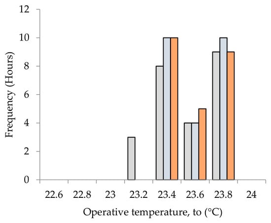
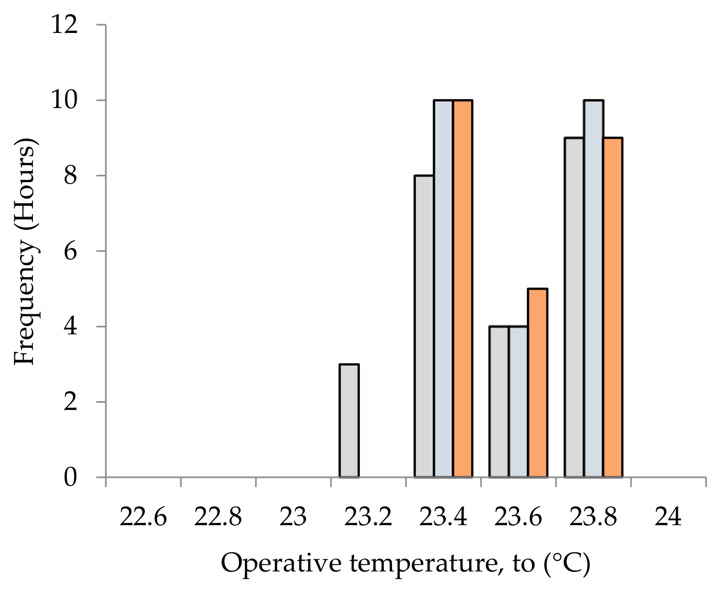
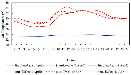
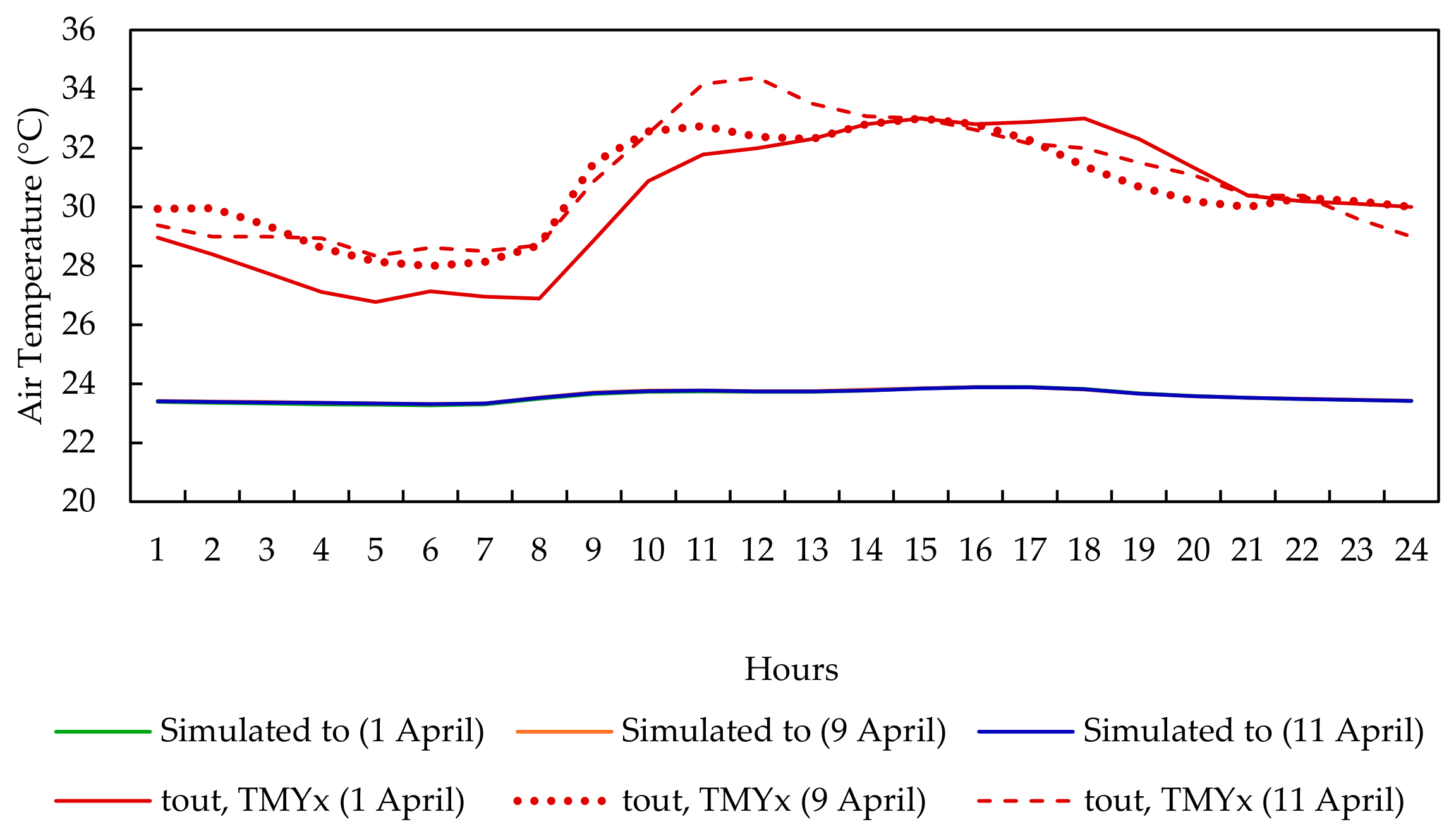
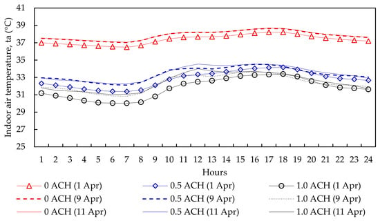
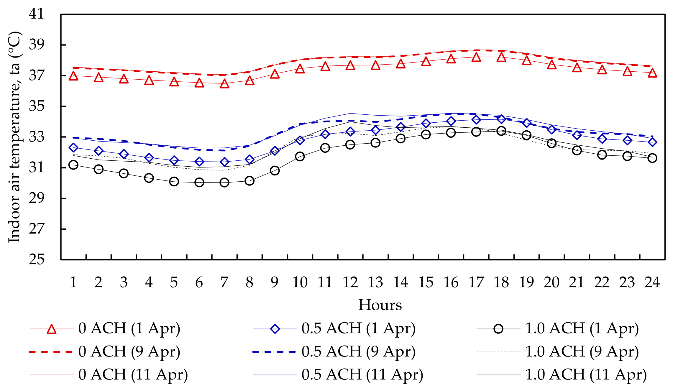
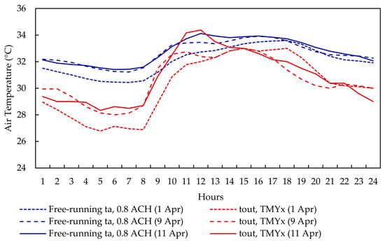
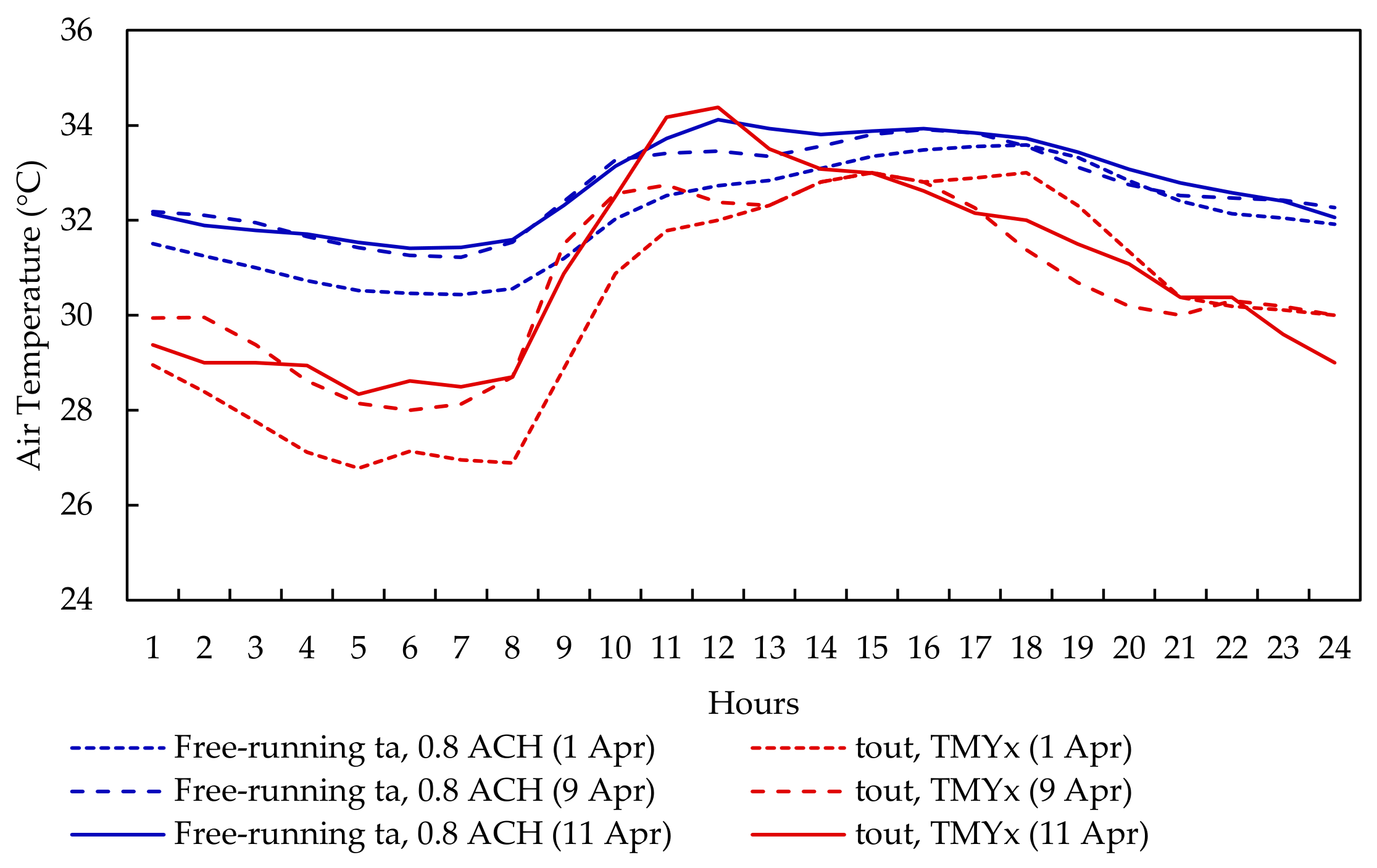
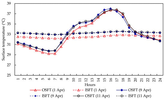
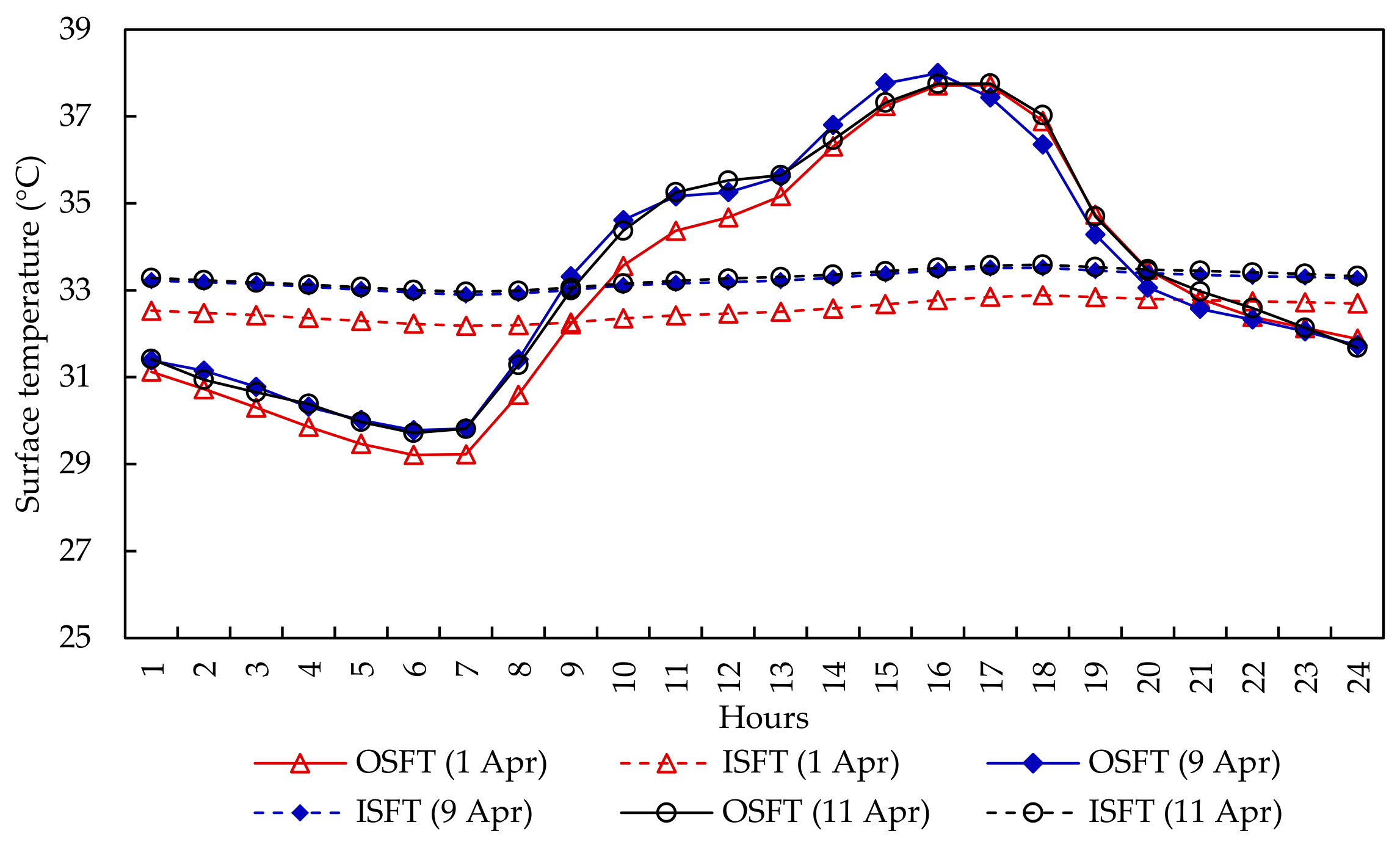
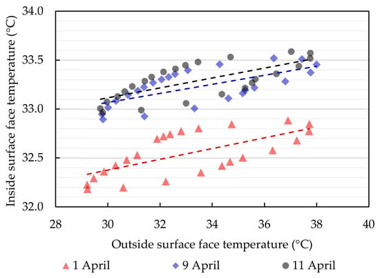
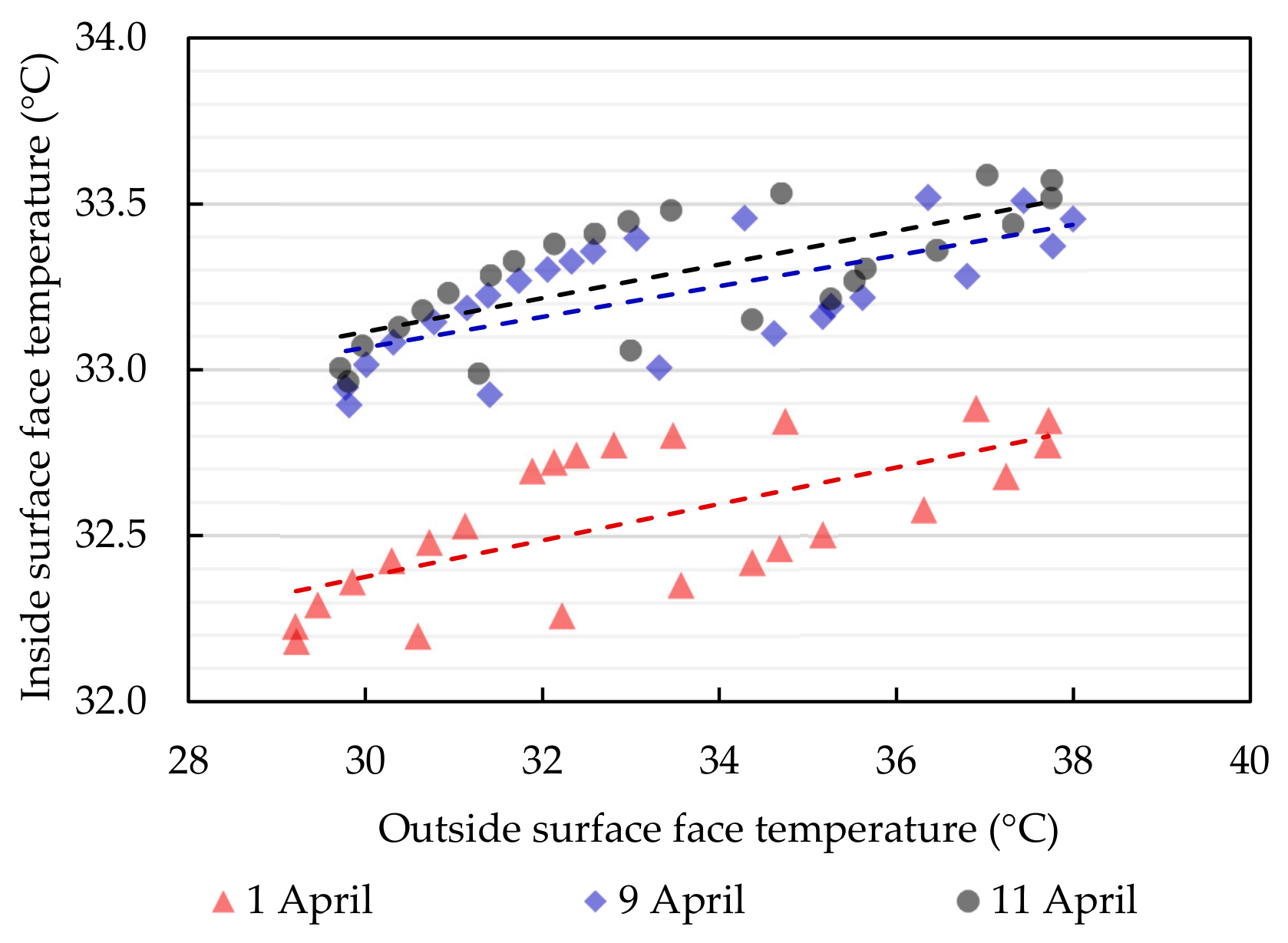
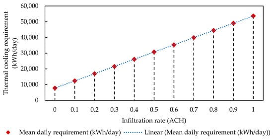
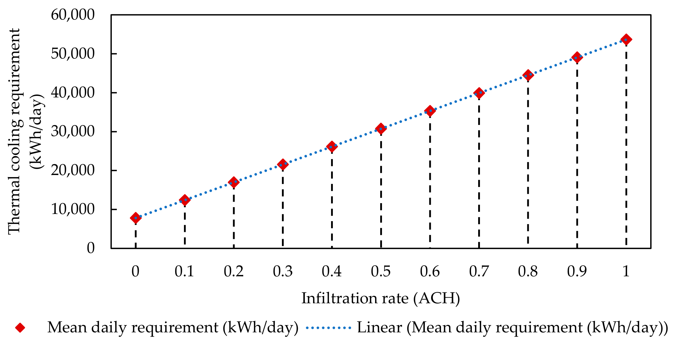
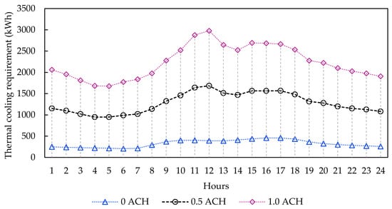
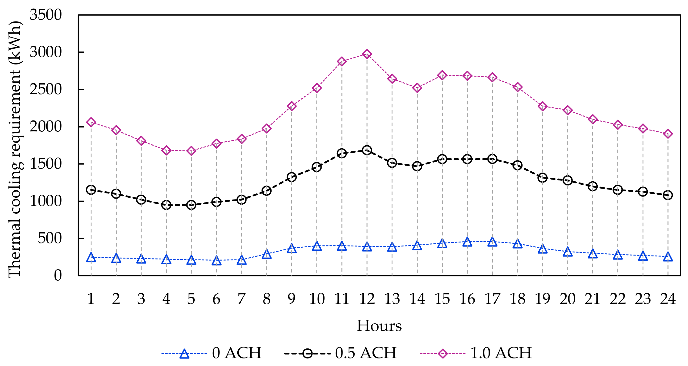
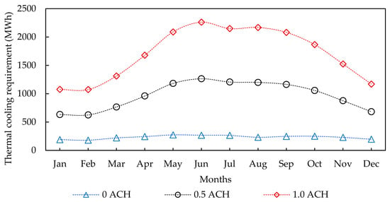
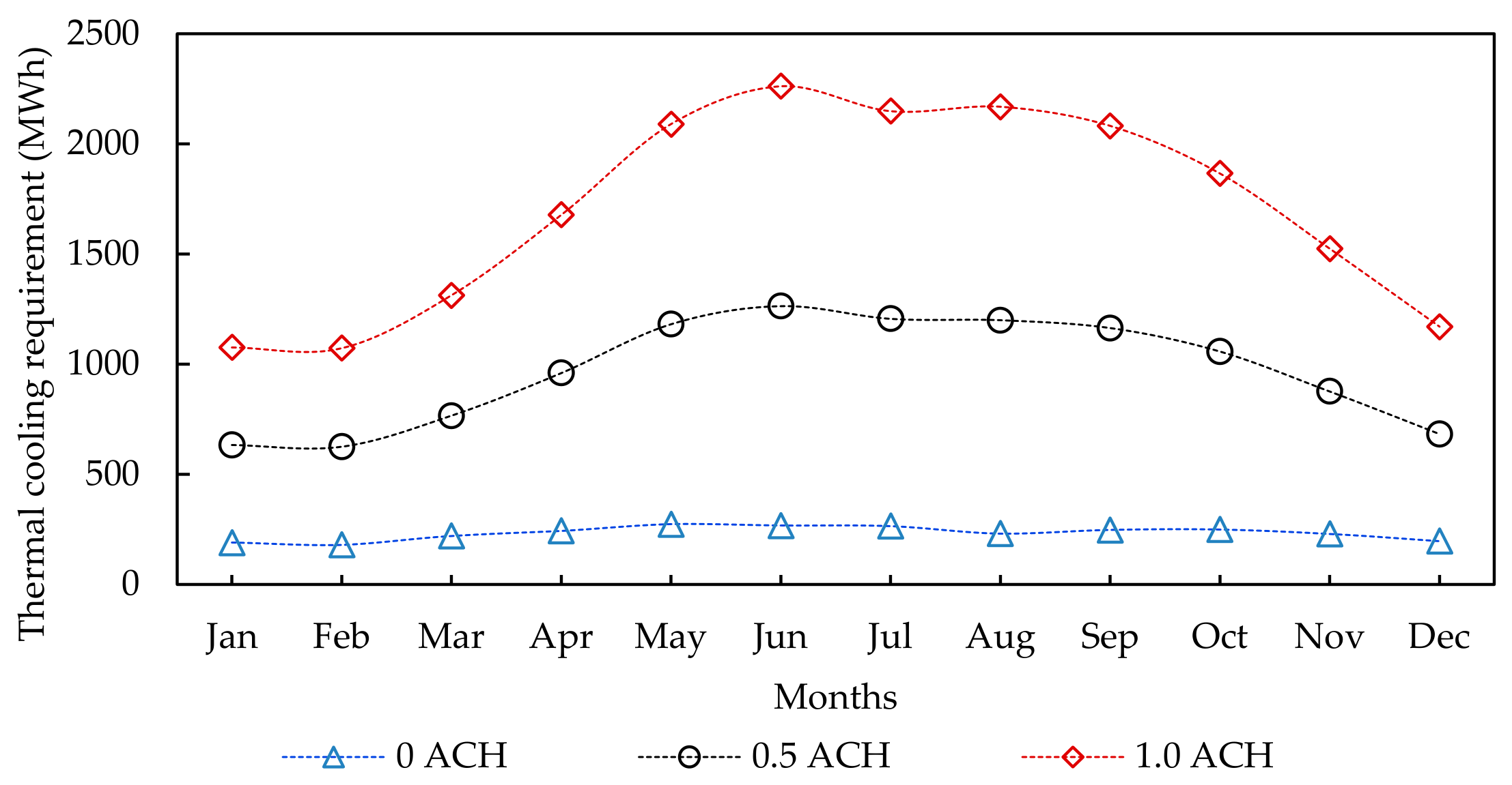

Disclaimer/Publisher’s Note: The statements, opinions and data contained in all publications are solely those of the individual author(s) and contributor(s) and not of MDPI and/or the editor(s). MDPI and/or the editor(s) disclaim responsibility for any injury to people or property resulting from any ideas, methods, instructions or products referred to in the content. |
© 2026 by the author. Licensee MDPI, Basel, Switzerland. This article is an open access article distributed under the terms and conditions of the Creative Commons Attribution (CC BY) license.