


Abstract
In building energy calculations, outdoor airflow can be represented using fixed assumptions prescribed by regulations or weather-dependent empirical and pressure-network approaches, and the selected approach can affect the resulting energy demand. This study compares five approaches in a four-storey residential reference building: a prescribed floor-area-based outdoor airflow assumption used in a national thermal-insulation standard (M1), two empirical infiltration models (M2–M3), and two AirflowNetwork models using analytical–tabulated or wind-tunnel-derived pressure coefficients (M4–M5). Six representative cities were simulated with typical meteorological year (TMYx) files based on 2009–2023 data and regional envelope configurations. Relative to M1, M5 produced higher annual outdoor airflow in two climate conditions and lower airflow in four, while increasing cooling demand by 0.97–14.48% in all conditions. With an identical leakage network and 15° wind-direction intervals, M5 produced annual air-change rates and heating demands 3.40–4.17% and 2.26–10.98% higher than M4, respectively. The effects of airflow-model selection therefore depend on climatic conditions and the heating or cooling component considered. These findings highlight the importance of interpreting differences between simplified standard outdoor-air assumptions and detailed airflow models in relation to the scope and underlying assumptions of each approach.
1. Introduction
In building energy performance calculations, outdoor air intake is one of the key determinants of sensible heat loss during the heating period, and of both sensible and latent heat loads during the cooling period [1]. Interzonal airflow and air exchange through natural or mechanical ventilation influence building energy consumption [2]. Natural ventilation (NV) can improve indoor thermal comfort and air quality while reducing energy consumption [3]. In particular, NV effectiveness should be verified during the design phase [4]. Various tools and metrics are used for this purpose [5]. These tools can range from simple approaches, such as analytical equations, to complex and comprehensive approaches, such as Computational Fluid Dynamics (CFD) [6].
Outdoor air can also enter buildings through unintended leakage paths in the building envelope, influencing heating and cooling energy requirements [2]. Standards-based simplified approaches operate on the basis of the building’s floor area or a prescribed constant flow rate [1]. Empirical infiltration models directly account for the effects of temperature difference and wind speed [2], whereas pressure-network-based models account for the directional pressure distribution on building surfaces and the mass balance among flow paths [7,8]. Therefore, for the same building and climatic conditions, the model form selected can alter the annual mean air change rate and the energy requirement.
In pressure-network-based airflow models, the wind pressure coefficient (Cp) is an important input for defining external pressure boundary conditions [3]. The Cp values used in building energy simulations can be obtained through full-scale field measurements on actual buildings. However, these measurements are costly, complex, and time-consuming [9]. As an alternative experimental method, wind tunnel testing enables Cp values to be determined using scaled building models under conditions in which wind speed, direction, and turbulence characteristics are controlled. Using Cp data obtained through these methods in airflow models enables the assessment of wind effects on outdoor air intake and building energy demand [10].
To illustrate how this relationship has been addressed using different modelling approaches, Table 1 presents a comparative overview of relevant studies, summarising their methods, key findings, and relevance to the present study.
Table 1.
Representative studies on airflow and infiltration modelling in buildings and the identified research gaps.
The studies summarised in Table 1 show that the source and definition of wind pressure coefficients influence airflow predictions [3,11,12], while the choice of infiltration model and calibration inputs affects the calculated air change rates and energy requirements [13,16,19,21]. These findings highlight the need to compare standards-based outdoor airflow assumptions and infiltration models under consistent building and climatic conditions. Such a comparison should also distinguish the effects of model selection from those of pressure-coefficient representation within airflow-network models.
Previous studies have generally examined simplified outdoor-air assumptions, empirical infiltration models, or pressure-network approaches separately. Controlled comparisons of these approaches across different climates using the same building and operating conditions remain limited, particularly when the influence of the pressure-coefficient source is isolated. This study compares five airflow modelling approaches across six climatic conditions within a common EnergyPlus framework. The matched M4–M5 analysis, fixed-envelope control, and sensitivity analyses separately evaluate the effects of pressure-coefficient representation, climate, building envelope, and leakage-network assumptions.
2. Materials and Methods
The study was conducted using an EnergyPlus-based comparative simulation approach involving a reference residential building, conditions representing Türkiye’s six climate regions, and five different outdoor airflow modelling approaches. Baseline comparisons were supplemented by controlled sensitivity analyses examining the effects of wind pressure coefficient representation and leakage-network assumptions. The following subsections describe the research design, reference building, climatic inputs, mathematical formulations of the airflow models, processing of TPU wind pressure data, conversion and allocation of prescribed leakage parameters, simulation settings, and calculation of airflow and energy performance indicators.
2.1. Research Design
The overall study design combined baseline model comparisons with controlled sensitivity analyses (Figure 1). Five modelling approaches—the floor-area-based outdoor airflow assumption prescribed for residential buildings by Türkiye’s national thermal-insulation standard, TS 825:2024 [1] (M1); two empirical infiltration models (M2–M3); and two AirflowNetwork models (M4–M5) were compared across six climate regions, yielding 30 baseline model–climate combinations. For a given climate, all building and operational inputs other than the airflow-modelling approach were held constant in the baseline comparisons. M2–M5 were assigned a common external-envelope airtightness target, whereas M1 followed its standard-prescribed airflow assumption, independent of airtightness. M4 and M5 used analytical–tabulated pressure coefficients and experimental wind-tunnel pressure coefficients from Tokyo Polytechnic University (TPU), respectively, within identical leakage networks and common 15° wind-direction intervals, isolating the effect of pressure-coefficient representation. Sensitivity analyses additionally examined envelope airtightness, the pressure–flow exponent, the roof share of total envelope leakage, and inter-floor airflow connections; each sensitivity scenario was evaluated relative to its corresponding baseline configuration. Model outputs comprised the annual mean air change rate calculated at reference density (ACHref), annual heating and cooling energy requirements, and their sum, reported as total thermal demand. The scope was limited to building-envelope infiltration and the standard-prescribed outdoor airflow assumption; window opening and intentional natural ventilation were excluded. The resulting airflow and energy predictions were not validated against full-scale field measurements; the findings therefore represent model comparisons and input-sensitivity assessments under the investigated conditions.
Figure 1.
Research workflow for baseline comparisons of outdoor airflow models and controlled sensitivity analyses. Research workflow for baseline airflow-model comparisons and sensitivity analyses. M1 follows TS 825:2024 [1], and arrows show the progression from common inputs to modelling, analysis, and performance evaluation.
M1 is a prescribed constant outdoor-airflow assumption based on floor area and is independent of building airtightness and weather conditions. M2 uses the Sherman–Grimsrud effective-leakage-area formulation, while M3 uses the AIM-2 flow-coefficient formulation to represent wind- and temperature-driven infiltration. M4 and M5 are AirflowNetwork approaches that solve pressure and mass balances; M4 uses analytical façade and tabulated roof pressure coefficients, whereas M5 uses area-weighted pressure coefficients derived from wind-tunnel measurements.
2.2. Reference Building
The reference building was developed from experimental model g080600 in the aerodynamic database of Tokyo Polytechnic University (TPU) [22]. Its square plan and flat roof were retained because experimentally measured surface-pressure coefficients were available for this precisely documented geometry. The TPU geometry therefore provides a controlled aerodynamic reference, while the storey arrangement, thermal zoning, glazing, operating conditions, and regional thermal-envelope properties were defined for the present residential energy model. Figure 2 presents the building geometry and envelope layers, and Table 2 summarises the geometric and glazing parameters. Each storey was represented as a conditioned thermal zone. The building north axis was fixed at 0°, and the outward-normal azimuths of the north, east, south, and west façades were 0°, 90°, 180°, and 270°, respectively. This orientation was maintained in all cities and models. Windows remained closed, and façade leakage was represented by equivalent cracks in the AirflowNetwork models. The building was modelled in isolation without surrounding buildings, eaves, balconies, external shading devices, a basement, an attic, or additional unconditioned spaces.
Figure 2.
(a) Reference building; (b) flat roof; (c) external wall; and (d) ground-floor slab.
Table 2.
Geometric and glazing parameters of the reference building.
2.3. TS 825:2024 and Regional Building Envelope Properties
TS 825:2024 defines the calculation principles for net heating and cooling energy requirements and thermal insulation design in buildings and divides Türkiye into six climate regions [1]. The geographical distribution of these regions and the representative cities selected for this study are shown in Figure 3. Research examining the updated envelope requirements highlights the importance of regional differences in assessing energy and environmental performance [23]. Insulation design is also influenced by climatic heating and cooling requirements, material properties [24], and the distribution of glazed and opaque façade areas [25]. In this study, the U-values recommended in TS 825:2024 were adopted as design targets for the regional envelope configurations.
Figure 3.
Climate-region classification of Türkiye according to TS 825:2024 [1] and locations of the representative cities selected for the analysis.
The six regional configurations are denoted CR1–CR6, corresponding respectively to Antalya, İzmir, İstanbul, Ankara, Sivas, and Erzurum.
2.3.1. Regional Building Envelope Design
Wall and roof insulation was assessed using the thermal resistance method described in Section 5.3 of TS 825:2024 [1]. The combined thermal resistance of the non-insulation layers and internal and external surfaces, denoted by , was calculated using Equation (1):
The thermal transmittance of each wall or roof element was then calculated using Equation (2), which includes the resistance of the adopted insulation layer [1].
The minimum insulation thickness was calculated using Equation (3), obtained by rearranging Equation (2) subject to ≤ .
Here, k identifies the wall or roof element, r the climate region, and j a material layer of element k; the subscript ins denotes insulation. dj and λj are the thickness (m) and thermal conductivity [W/(mK)] of each non-insulation layer, respectively. Rsi,k and Rse,k are the internal and external surface thermal resistances [m2K/W]. The non-insulation layers and surface resistances were held constant across regions for each element, so R0,k is independent of r.
The adopted insulation thickness is denoted by dins,k,r, its thermal conductivity by λins, and the calculated minimum thickness by dins,min,k,r. All thicknesses in Equations (1)–(3) are expressed in metres. Uk,r and Utarget,k,r denote the calculated and regional target thermal transmittances, respectively, both in W/(m2K). The calculation inputs are presented in Table 3, while the minimum wall and roof insulation thicknesses and the calculated and target U-values are summarised in Table 4. The wall and roof insulation thicknesses shown in Figure 2 satisfy the calculated minimum requirements.
Table 3.
Inputs used in the thermal calculations for the building envelope.
Table 4.
Minimum wall and roof insulation thicknesses and regional U-value checks [1].
The ground-contact slab was assessed using the geometry-dependent method specified in Section 6.6.2 of TS 825:2024 [1]. The equivalent thickness for each climate region, , was calculated using Equation (4).
Here, is the total external-wall thickness, including insulation, in region (m), and is the soil thermal conductivity [W/(mK)]. and are the surface thermal resistances used for the ground-contact slab [m2K/W]. The summation in Equation (4) includes all slab layers, including insulation; is the thickness of slab layer in region (m), and is its thermal conductivity [W/(mK)]. The equivalent thickness is expressed in metres.
Because in all six climate regions, the characteristic floor dimension and the corresponding ground-floor thermal transmittance were calculated using Equation (5), following Section 6.6.2 of TS 825:2024 [1].
Here, is the ground-contact floor area (m2), is the exposed perimeter (m), and is the characteristic floor dimension (m). denotes the steady-state thermal transmittance of the ground-contact floor in climate region [W/(m2K)], accounting for heat spreading through the ground, and denotes the natural logarithm. The resulting -values are reported in Table 4.
Table 4 summarises the calculated minimum insulation thicknesses for the external walls and roof and compares the U-values of the adopted wall, roof and ground-floor constructions with the regional targets specified in TS 825:2024 [1]. The insulation thicknesses shown in Figure 2 yield U-values that satisfy the corresponding targets in all six climate regions. The ground-floor U-values provide a steady-state assessment that accounts for heat spreading through the ground. Annual ground heat transfer was simulated using the Kiva model integrated into EnergyPlus, which accounts for two-dimensional transient heat conduction through the slab, foundation and surrounding soil [26].
Building geometry was held constant across all model–climate combinations, while the thermal properties of the building envelope were specified according to regional design targets. For each city, these envelope properties were held constant across M1–M5, enabling a controlled assessment of the effect of the airflow modelling approach. Accordingly, model comparisons within each city were conducted under common envelope conditions, whereas comparisons between cities reflected simultaneous changes in climatic conditions and regional envelope properties.
2.3.2. Climate Data and Meteorological Boundary Conditions
Annual simulations used typical meteorological year (TMYx) files based on 2009–2023 hourly meteorological data and supplied in EnergyPlus Weather (EPW) format for the cities listed in Table 5. The files were generated using typical-year selection procedures consistent with TMY/ISO 15927-4:2005 methodologies. Each file is a composite 8760 h year assembled to represent typical conditions rather than a specific calendar year. Outdoor temperature, humidity, atmospheric pressure, solar radiation, wind speed, and wind direction were used as meteorological inputs. The same city-specific EPW file was applied to M1–M5 within each city. TMYx files do not represent interannual variability or extreme weather events.
Table 5.
EPW weather files used for the reference cities.
2.4. TPU Aerodynamic Database and Experimental Data
Point pressure-coefficient records for the flat-roofed g080600 model without eaves, obtained from the Tokyo Polytechnic University (TPU) aerodynamic database, were used to generate the wind pressure inputs for M5 [22]. The experimental and sampling characteristics are summarised in Table 6. Figure 4a shows the distribution of pressure taps across the building surfaces, while Figure 4b presents the surface and wind-direction mapping between TPU and EnergyPlus. Wind directions in EnergyPlus identify where the wind comes from, whereas the straight arrows in the figure indicate the direction of airflow.
Table 6.
Experimental, sampling and directional mapping characteristics of the TPU dataset used in this study.
Figure 4.
TPU g080600 model: (a) unfolded building surfaces and pressure tap locations; (b) surface and wind-direction mapping between TPU and EnergyPlus.
2.5. Thermal and Airflow Modelling
Annual simulations were performed in EnergyPlus 25.1.0 [1] using a heat and mass balance approach [33]. Air was assumed to be well mixed within each thermal zone, and heating and cooling demands were calculated using ZoneHVAC:IdealLoadsAirSystem [1] with unlimited capacity to maintain the specified temperature setpoints. Both humidification and dehumidification control types were set to None in all models. Within each city, identical envelope properties, meteorological inputs and operating schedules were used for M1–M5. The common thermal inputs and ground heat transfer assumptions are summarised in Table 7.
Table 7.
Common thermal model and operating inputs.
The operating and soil properties were held constant across all airflow models within each climatic condition. Constant setpoints, occupancy, and internal heat gains were adopted to provide common and controlled operating conditions and to avoid introducing schedule-dependent variability into the model comparison.
No fixed heating or cooling season was prescribed. Heating and cooling were available throughout the 8760 h annual simulation at constant setpoints of 20 and 26 °C, respectively. Annual heating and cooling demands were calculated by separately summing the corresponding hourly Ideal Loads outputs.
Outdoor airflow was represented using the five approaches defined in Table 8. In M1, the area-specific rate of 0.7 m3/(hm2) prescribed in TS 825:2024 for apartment-building energy calculations was multiplied by the conditioned floor area and distributed equally among the zones [1]. This value is a constant floor-area-based outdoor-airflow assumption; it is not an air-change rate or a physical infiltration model derived from a specified airtightness level, and it does not vary with wind speed or indoor–outdoor temperature difference. M2–M5 instead represent infiltration as a function of envelope airtightness and weather-related driving forces.
Table 8.
Airflow models and inputs used in the main scenario.
For M2–M5, a common envelope airtightness of and a flow exponent of were specified. These values define the comparison scenario adopted in this study. The conversion based on the pressure–flow power law was performed using Equations (6)–(8) [34].
Here, is the total volumetric flow rate at a pressure difference of 50 Pa (m3/s); V is the building air volume (m3); is the volumetric flow coefficient [m3/(sPan)]; is the mass flow coefficient [kg/(sPan)]; and is the reference pressure difference of 50 Pa. The reference air conditions were 20 °C, 101,325 Pa and zero humidity ratio, giving . The effective leakage area used in M2, referenced to 4 Pa and expressed in cm2, was obtained using Equation (9).
Here, is the discharge coefficient of the reference orifice and was set to unity when defining the effective leakage area at 4 Pa [35]. This convention does not imply a unit discharge coefficient for the physical leakage paths. The factor (104) converts m2 to cm2. No additional discharge coefficient was applied to the AFN crack coefficients.
The M1–M3 objects belong to the ZoneInfiltration group. The stack and wind coefficients in M2 and M3 were used with the unit conventions of their respective model definitions [2]. In M2, is used to derive the effective leakage area; the object has no independent flow exponent input.
In M2 and M3, each of the first three zones was assigned 18.75% of the envelope leakage inputs, while the uppermost zone, including the roof contribution, was assigned 43.75%. Each zone was represented as an independent single-storey infiltration subsystem without a chimney, using the coefficients for a slab-on-grade configuration in M3. Although these formulations include wind- and temperature-driven infiltration, they do not directly solve the pressure coupling and combined vertical airflow between storeys. M4 and M5 instead use a multizone pressure and mass-balance solution. Differences between M2/M3 and M4/M5 may therefore reflect both model formulation and the representation of pressure distribution and inter-storey airflow.
Here, and are the zone volumetric outdoor air flow rates (m3/s); and are the zone and outdoor air temperatures (°C); is the local wind speed (m/s); and is the shelter factor. and denote the stack and wind coefficients, respectively, with subscripts 2 and 3 identifying the corresponding model. In Equation (10), the leakage area is expressed in cm2, and the divisor of 1000 accounts for the conversion from L/s to m3/s.
In M4 and M5, pressures arising from wind and temperature differences were solved together with the zone mass balances. This AFN approach couples the flow rates through the connections to the zone heat and moisture balances [36]. Both models used 16 façade connections and one roof connection. Of the total envelope leakage coefficient, 25% was assigned to the roof and the remainder was distributed equally among the 16 façade connections. No airflow connections between storeys were included in the main scenario. The reference pressure–flow relationship for the connections and the zone mass balance are expressed in Equation (12).
Here, is the fraction of the total leakage coefficient assigned to connection ; is the pressure difference across that connection (Pa); is the set of connections associated with zone ; and is the mass flow rate (kg/s), signed relative to the zone. EnergyPlus adjusts the reference coefficients according to the air properties during the simulation [8]. Consequently, a common does not require M2–M5 to produce identical flow rates under natural conditions.
The façade pressure coefficients for M4 were obtained by directly evaluating the Swami–Chandra correlation for a square plan at 15° intervals [37]. Wind directions were expressed as meteorological wind-from azimuths measured clockwise from north. The outward-normal azimuths of the north, east, south and west façades were 0°, 90°, 180° and 270°, respectively. For each façade, the incidence angle was defined as the smaller angular separation between the wind-from direction and the outward normal, ranging from 0° for normal windward incidence to 180° for normal leeward incidence. The ratio of each façade width to the adjacent façade width was unity for the square plan. For the roof, pressure coefficients were taken from the square-plan entry of the CPHighRiseRoof table in the EnergyPlus 25.1.0 source code [38]. EnergyPlus applies this roof table to both low-rise and high-rise rectangular buildings. The coefficients were −0.70, −0.55, −0.55 and −0.70 at 0°, 30°, 60° and 90°, respectively, with the sequence repeated every 90°. Intermediate values were obtained by linear interpolation to construct the common 15° wind-direction series. In M5, the time-averaged values at the TPU pressure taps were weighted by the areas of Voronoi cells clipped to the surface boundaries. The representative pressure coefficient for each surface was calculated using Equation (13).
Here, identifies the surface; is the set of pressure taps on that surface; is the area represented by tap (m2); is its time-averaged pressure coefficient; and is the wind direction. The area-weighting procedure was implemented in this study. Wind directions and surfaces were mapped as shown in Figure 4. The common 15° direction series obtained using rotational symmetry was closed by setting the value at 360° equal to that at 0°.
The AFN external nodes were positioned at the mid-storey heights on the façades and at the building height on the roof. Both models used a wind profile exponent of 0.20 and a boundary layer thickness of 450 m. To preserve the common pressure reference at roof height, the coefficients were transformed to the external node heights using Equations (14) and (15).
Here, H = 12 m, and z, α, ρ, and pw denote the reference height, external-node height, wind-profile exponent, operating air density, and wind-induced surface pressure, respectively. The transformation preserves the wind pressure referenced to roof height. In M5, the experimental tap values were area-weighted to obtain one representative pressure coefficient for each façade and this value was applied to all storeys. This preserves the experimentally observed differences among façades but does not represent vertical pressure variation along an individual façade. Storey-specific pressure coefficients could therefore alter the inter-storey airflow distribution, particularly when wind and stack effects are both important, and constitute a potential direction for future research.
2.6. Sensitivity Analyses and Comparative Experiments
Three sensitivity experiments for M4 and M5 and an additional fixed-envelope control for M1–M5 were conducted in the six reference cities (Table 9). Within each of the three M4–M5 sensitivity experiments, the EPW file, regional envelope, operating schedules, Kiva model, and all non-varied inputs were held at their baseline values. In the separate fixed-envelope control, the city-specific EPW files were retained, whereas the opaque-envelope and glazing properties were replaced by the CR3 Istanbul configuration in all six cities, as described below.
Table 9.
Scope of the sensitivity analyses and comparative experiments.
In the 324-condition experiment, the roof received the fraction of the total external leakage coefficient and the remainder was divided equally among the 16 façade connections according to Equation (16).
Three connections linked adjacent storeys, with the coefficient of each connection defined by Equation (17).
The baseline airtightness level was = 4 h−1. Values of = 2 and 6 h−1 were selected as controlled sensitivity bounds representing relatively more airtight and more air-permeable envelope conditions, respectively. For engineering context, Cardoso et al. [35] examined residential levels of 0.6, 3.0, 6.0, and 11.5 h−1 and identified 3.0 and 6.0 h−1 as mid-range requirements for dwellings with mechanical extract and natural ventilation, respectively. The present 2–6 h−1 range therefore spans airtightness levels comparable in order of magnitude to residential scenarios reported in the literature, from a relatively airtight case to a more air-permeable case; it is not presented as a measured statistical distribution for the Turkish building stock. The inter-floor connection multiplier = 0 denotes no internal connection, while = 1 and 10 define progressively increased internal pressure coupling.
For the pressure-coefficient experiment, M4 and M5 were evaluated at 15° and 30°. M4 façade coefficients were calculated directly at both intervals; intermediate roof values were linearly interpolated, and the M5 30° series was sampled from its 15° series. In the flow-exponent experiment, and were recalculated for each using Equations (7) and (8), preserving h−1 and the reference flow at 50 Pa; , and the 15° direction interval were retained.
An additional fixed-envelope control was performed for M1–M5 using the six city-specific EPW files, yielding 30 annual conditions. The opaque-envelope constructions, material properties, layer order, insulation thicknesses, glazing U-value and SHGC were fixed at the CR3 Istanbul configuration across all six cities. Building geometry, operating schedules, model-specific airflow settings and the Foundation:Kiva ground heat-transfer method were retained at their baseline values. Therefore, within each airflow model, the remaining inter-city differences primarily reflect the selected city-specific weather files, including their influence on the weather-dependent ground boundary conditions, rather than regional changes in the envelope or glazing properties. This control examined whether the inter-city pattern of model differences persisted when regional envelope differences were removed. Its interpretation is conditional on the CR3 Istanbul envelope and the six selected weather files.
Foundation:Kiva was fixed in all principal M1–M5 comparisons. The alternative monthly ground-temperature method was evaluated only in a separate controlled M1–M5 sensitivity comparison, with all other building and airflow inputs unchanged.
2.7. Simulation Outputs and Comparative Metrics
The simulations were compared using the annual mean inward outdoor-airflow rate expressed as reference-density air changes per hour () and specific heating, cooling and total thermal demands. EnergyPlus 25.1 output definitions were used [33,39]. Heating and cooling demands were obtained from the Zone Ideal Loads Supply Air Total Heating Energy and Zone Ideal Loads Supply Air Total Cooling Energy outputs, respectively, which include sensible and latent components. For M1–M3, zone infiltration mass-flow rates were summed; for M4–M5, only inward flows through external AFN connections were included. Inter-zone and outward flows were excluded. The resulting was calculated using Equation (18). This metric provides a common one-way outdoor-air-inflow basis across the model groups. Net and absolute bidirectional AFN flows were not used because they do not correspond to the unidirectional infiltration rates imposed through the ZoneInfiltration objects in M1–M3.
Here, , m3 and kg/m3. The conditioned floor area was m2. Specific heating demand was calculated using Equation (19).
Specific cooling demand was calculated using Equation (20).
Specific total thermal demand was calculated using Equation (21).
For any metric X, the relative difference was calculated using Equation (22).
M1 was the reference for the principal five-model comparison and M4 for pressure-coefficient comparisons. Each annual run was checked for 8760 unique hourly records, finite outputs, successful completion and no severe or fatal errors; AFN zone mass balances were also checked.
2.8. Effect Sizes and Variance Decomposition
For each matched case, the signed difference in the original unit was calculated using Equation (23).
For each matched M4–M5 case, the percentage difference was calculated using Equation (22), with M4 as the reference. The mean values reported in Table 10 are the arithmetic means of the 27 case-wise percentage differences for each city, giving equal weight to each matched case. Separately, aggregate percentage differences across the specified matched set were calculated using the ratio-of-sums formulation in Equation (24).
Table 10.
Minimum, maximum, and arithmetic mean of the M5–M4 percentage differences across the 27 matched sensitivity cases in each city, with M4 as the reference.
The variance-decomposition framework separates output variability into contributions from individual factors and their interactions [40,41]. In this study, variance decomposition was applied separately to annual mean and the specific heating, cooling, and total thermal demands. The factors were city/regional envelope, pressure-coefficient representation (M4 and M5), envelope airtightness (, 4, and 6 ), roof leakage fraction (, 0.25, and 0.50), and inter-floor connection multiplier (, 1, and 10). Combining all factor levels produced a complete, equally weighted factorial design comprising 324 conditions. The pressure-flow exponent (), Foundation:Kiva ground model, and 15° wind-direction interval were held constant in all conditions.
For each output, an orthogonal factorial ANOVA decomposition was applied to the 324 equally weighted simulations, retaining all interactions through the fifth order. Effect components were obtained recursively from marginal means by subtracting the grand mean and all constituent lower-order effects. Each was calculated as the sum of squared component values over all 324 conditions; was the total sum of squared deviations from the grand mean.
The main-effect and interaction-inclusive shares of factor were calculated as:
Here, denotes a non-empty subset of factors, and is the main-effect sum of squares for factor . Equation (26) includes all components containing . Results are reported as and , respectively; the latter are not additive across factors. These variance-based sensitivity indices are conditional on the tested factor levels and their equal weighting [42]. The full decomposition is saturated, with zero residual degrees of freedom; no significance tests were performed.
2.9. Modelling Assumptions and Methodological Scope
The principal modelling assumptions defining the scope and interpretation of the comparative framework were as follows:
- M5 was a TPU-informed pressure-coefficient model and was not treated as ground truth or as a calibrated representation of a monitored building.
- Area-weighted façade pressure coefficients were applied to all storeys; local vertical and horizontal pressure variations were therefore not represented.
- The directional pressure-coefficient series was generated using rotational symmetry and, where required, linear interpolation. Consequently, the analysis compared the defined pressure-coefficient representation chains rather than the complete spatial variability of surface pressures.
- Building orientation was fixed for all cities and airflow approaches.
- The investigated levels, roof-leakage fractions, and inter-floor connection levels were controlled sensitivity inputs rather than measurements of a specific building. The = 2, 4, and 6 h−1 cases represent relatively more airtight, baseline, and more air-permeable conditions within the sensitivity design.
- The inter-floor airflow coefficients did not represent measured door, stairwell or shaft geometries.
- The city/regional-envelope factor combined weather and envelope effects, with each climate region represented by one city and one TMYx weather file.
- The Kiva soil properties were modelling assumptions and were not calibrated using site-specific ground measurements.
- The Ideal Loads outputs represented heating and cooling thermal demand rather than electricity or fuel consumption.
- The reported variance shares were descriptive and conditional on the selected factor levels and equal scenario weights.
- The constant setpoints and internal-gain assumptions were adopted for controlled comparison and do not represent time-varying residential operation; the quantitative energy results are conditional on these operating assumptions.
3. Results
3.1. Simulation Verification, Quality Control, and Evidence Supporting Model Reliability
For the transfer of TPU data to the AirflowNetwork, the surface assignments of the 232 pressure taps, surface-area totals, directional transformations, 360–0° closure, and pressure-coefficient tables for the 17 external nodes were checked; no missing or duplicate records were identified. Pressure and height transformations were also evaluated independently of the actual M4 and M5 linkage networks. The maximum differences between the independent calculation and the EnergyPlus results were 2.57 × 10⁻⁴ Pa for external-node pressure and 4.64 × 10⁻⁶ kg/s for linkage mass-flow rate. The difference between the wind pressures calculated using the two reference heights remained below 3.56 × 10⁻¹⁵ Pa.
For all reported annual simulations, 8760 unique hourly records, finite output values, successful simulation completion, and the absence of Severe or Fatal errors were confirmed. The AFN zone mass balances satisfied the prescribed tolerance. The maximum annual signed closure residual of the hourly zone-air heat balance was 0.00233 kWh/m2, while the maximum integral of the absolute residual was 0.106 kWh/m2. The quality-control results are summarised in Table 11.
Table 11.
Summary of simulation verification and quality-control results.
The mass- and heat-balance checks, independent pressure and mass-flow calculations, and comparisons with published model-based studies [43,44,45] support the numerical consistency and physical plausibility of the implementation. In addition, M5 retained a 1.765–7.386% higher annual than M4 across all 162 matched sensitivity cases.
3.2. Pressure-Coefficient Representations
The pressure coefficients presented in Figure 5 are surface-mean values. The reference wind speed used to calculate the coefficients was defined at the building height, corresponding to a full-scale height of H = 12 m in the TPU wind-tunnel model. Panel (a) compares the M4 and M5 coefficients for the S1 west façade, which is directly windward at 270°, while panel (b) presents the corresponding comparison for the S5 flat roof. The M4 façade series was obtained by evaluating the analytical expression at 15° intervals, while its roof series was based on tabulated coefficients with intermediate values obtained by linear interpolation. The M5 series comprises surface-area-weighted coefficients derived from the TPU g080600 measurements and transformed to 24 EnergyPlus wind directions (Table S4).
Figure 5.
Pressure-coefficient representations: (a) S1 west façade; (b) S5 flat roof.
Examination of Figure 5 reveals that the analytical–tabulated representation used in M4 and the TPU measurement-derived representation used in M5 produced broadly similar windward–leeward patterns but differed in both coefficient magnitude and directional variation. For the west façade, the M4 coefficients ranged from −0.681 to 0.603, whereas the M5 coefficients ranged from −0.742 to 0.702. M4 reached its maximum positive coefficient at 270°, while the M5 maximum occurred at 285°. At 270°, the M4 and M5 coefficients were 0.603 and 0.654, respectively, corresponding to an M5 − M4 difference of 0.050. Across the 24 unique wind directions, the signed differences ranged from −0.186 to 0.141, with a mean absolute difference of 0.062.
The flat-roof coefficients remained negative at every direction. The M4 series ranged from −0.700 to −0.550, whereas the M5 series occupied the narrower range from −0.712 to −0.639. Direction-specific M5 − M4 differences ranged from −0.106 to 0.003, and the mean absolute difference was 0.078. Compared with the piecewise-linear directional variation of the M4 roof coefficients, M5 exhibited a narrower but recurring directional suction pattern. Thus, M4 and M5 did not represent wind-pressure differences among the surfaces identically, despite using the same leakage network.
3.3. Baseline Outdoor Airflow Across Models and Climate Regions
The baseline comparison was performed using n50,env = 4 h−1, froof = 0.25, β = 0, n = 0.67 and a 15° wind-direction interval. Figure 6 compares the annual mean outdoor air change rates at the reference density for M1–M5 across the six climate regions and reference cities. For M1–M3, zone infiltration inflows were included, whereas for M4–M5 only inward flows through external AirflowNetwork connections were considered.
Figure 6.
Baseline annual mean outdoor air change rates across the five airflow models and six climate regions.
Examination of Figure 6 reveals that the model ranking varied among the climate regions. The lowest ACHref was obtained with M3 in CR1 Antalya and CR3 Istanbul, M1 in CR2 Izmir, and M4 in CR4 Ankara, CR5 Sivas and CR6 Erzurum. M3 values ranged from 0.127 h−1 in CR5 Sivas to 0.239 h−1 in CR2 Izmir. In contrast, M1 produced the highest value in CR1 Antalya, CR4 Ankara, CR5 Sivas and CR6 Erzurum, whereas M5 produced the highest value in CR2 Izmir and CR3 Istanbul.
M1 exhibited comparatively limited regional variation, with ACHref ranging from 0.197 to 0.232 h−1. Wider ranges occurred for the weather-dependent models: 0.116–0.257 h−1 for M4 and 0.120–0.268 h−1 for M5. Both AirflowNetwork models produced their highest annual mean outdoor air change rates in CR2 Izmir and their lowest values in CR5 Sivas.
Whether M5 produced a higher or lower than M1 depended on the climate region. M5 exceeded M1 by 16.78% in CR2 Izmir and by 12.89% in CR3 Istanbul, but was 20.61–39.35% lower in the other four cities. By contrast, M5 remained higher than M4 in every city, with differences ranging from 3.40% to 4.17%.
3.4. Baseline Heating and Cooling Demands
Annual specific heating, cooling and total thermal demands under the baseline conditions are compared in Figure 7. The figure presents the results of M1–M5 for the six climate regions. Heating and cooling values represent the thermal demands calculated by the Ideal Loads system and should not be interpreted as electricity or fuel consumption.
Figure 7.
Baseline thermal demands: (a) annual heating; (b) annual cooling; (c) total heating and cooling.
Examination of Figure 7 reveals that the most pronounced variation among the climate regions occurred in the relative contributions of heating and cooling. Annual specific heating demand generally increased from the warmer to the colder regions, whereas cooling demand decreased in the same direction. All models produced the highest cooling demand in CR1 Antalya and the highest heating demand in CR6 Erzurum. Under the baseline city–regional-envelope configurations, cooling demand remained higher than heating demand in every city examined.
The ranking of the models by heating demand varied with climate region. M5 produced the highest heating demand in CR1 Antalya and CR3 Istanbul, M2 in CR2 Izmir and CR5 Sivas, and M1 in CR4 Ankara and CR6 Erzurum. Relative to M1, the M5 heating demand was 31.02–180.91% higher in CR1–CR3 and 16.45–32.58% lower in CR4–CR6. The large relative differences in CR1 Antalya and CR2 Izmir resulted from the small annual heating demands, which ranged from only 0.440 to 1.235 kWh/m2 and from 1.114 to 2.029 kWh/m2, respectively. Percentage differences in these regions should therefore be considered together with the corresponding absolute values.
Cooling demand showed a smaller, but climate-dependent, response to the airflow-model representation. M5 produced higher cooling demand than M1 in every city, with the difference increasing from 0.97% in CR1 Antalya to 14.48% in CR5 Sivas. By comparison, the M5–M4 differences remained between −0.73% and 0.06%; M5 produced marginally lower cooling demand than M4 in CR3–CR6.
For total thermal demand, M5 exceeded M1 by 2.13–8.65% in CR1–CR5 but was 6.11% lower in CR6 Erzurum. The total-demand differences between M4 and M5 were small in every climate region, ranging from −0.05% to 0.57%. This close agreement occurred because the changes in the heating and cooling components partly offset one another, despite the consistently higher outdoor air change rates obtained with M5 than with M4.
3.5. Matched Effect of Pressure-Coefficient Representation
To isolate the effect of pressure-coefficient representation, M4 and M5 were compared under otherwise matched modelling conditions. The two models used the same leakage network, flow exponent, weather data, and simulation settings, but differed in their external pressure-coefficient inputs: M4 used the analytical representation, whereas M5 used the TPU-derived representation. City-specific relative differences were calculated using Equation (22), with M4 as the reference.
Examination of Figure 8 shows that M5 produced higher annual than M4 in all six climate regions. The absolute increase ranged from 0.0040 to 0.0106 h−1, corresponding to relative differences of 3.40–4.17%. The narrow percentage range indicates that replacing the analytical pressure coefficients with the TPU-derived representation affected the annual air change rate consistently across the investigated climates.
Figure 8.
M5–M4 relative differences in (a) annual , (b) heating demand, (c) cooling demand, and (d) total thermal demand. Blue and orange markers indicate positive and negative differences, respectively.
Heating demand was also higher under M5 in every city. The absolute differences ranged from 0.122 to 0.305 kWh/m2, while the corresponding relative differences ranged from 2.26% in CR6 Erzurum to 10.98% in CR1 Antalya. Cooling demand showed a smaller and directionally mixed response: M5 produced slightly higher values in CR1 Antalya and CR2 İzmir, but slightly lower values in CR3–CR6. Across all cities, the cooling-demand differences ranged from −0.219 to 0.038 kWh/m2, or from −0.73% to 0.06%.
The resulting differences in total thermal demand remained limited, ranging from −0.025 to 0.294 kWh/m2 and from −0.05% to 0.57%. M5 increased total thermal demand in five cities and produced a marginal decrease only in CR4 Ankara. For the matched six-city set, the ratio-of-sums differences were 3.91% for annual , 3.75% for heating demand, −0.20% for cooling demand, and 0.22% for total thermal demand. Thus, the consistent increase in annual air change rate under M5 translated into a clearer increase in heating demand, whereas the smaller and opposing cooling-demand changes limited the net effect on total thermal demand.
3.6. Roof-Leakage Distribution and Inter-Floor Connection Sensitivity
To determine whether the effect of pressure-coefficient representation persisted under different leakage-network assumptions, M4 and M5 were compared across controlled sensitivity cases. These cases included three envelope airtightness levels (n50,env = 2, 4, and 6 h−1), three roof-leakage fractions (froof = 0, 0.25, and 0.50), and three inter-floor connection levels (β = 0, 1, and 10). This design produced 27 matched M4–M5 comparisons for each city and 162 matched comparisons across the six cities. The ranges reported in Table 10 represent the minimum and maximum values obtained across the controlled scenarios.
Examination of Table 10 shows that M5 yielded a higher annual than M4 in all 162 matched comparisons. City-specific relative differences ranged from 1.765% to 7.386%. This result shows that the increase in annual outdoor air change associated with the TPU-derived pressure-coefficient representation persisted when envelope airtightness, roof-leakage fraction, and inter-floor connection level were varied. However, the magnitude of the difference depended on both the leakage-network configuration and the climate region.
Heating demand was higher under M5 in 161 of the 162 comparisons. The only negative value occurred in CR2 İzmir and was limited to −0.001 kWh/m2, corresponding to −1.227%, which is negligible in absolute terms. In contrast, the direction of the cooling-demand difference depended on climate. Both positive and negative differences occurred in CR1–CR3, whereas M5 produced lower cooling demand in every matched case in CR4–CR6. The largest relative reduction, −1.574%, occurred in CR6 Erzurum.
Differences in total thermal demand remained more limited because the changes in heating and cooling demand partly offset one another. City-specific mean differences ranged from −0.003 to 0.369 kWh/m2, with a marginal mean decrease occurring only in CR4 Ankara. Expressed as relative differences, the city-specific means ranged from −0.007% to 0.688%. These results indicate that the direction of the M5 effect on annual was robust across the controlled leakage-network assumptions, whereas its effect on total thermal demand was smaller and could change direction because of the climate-dependent responses of the heating and cooling components.
To synthesize the joint sensitivity results and distinguish the relative contributions of the investigated factors, the variance of each output was decomposed using the procedure described in Section 2.8. The resulting main-effect and interaction-inclusive variance shares for and the annual heating, cooling, and total thermal demands are presented in Table 12.
Table 12.
Main-effect and interaction-inclusive variance shares for the 324-condition joint sensitivity design. Values in parentheses are interaction-inclusive shares (%).
Variance decomposition showed that annual mean variability was governed primarily by envelope airtightness. The main-effect share of was 57.29%, increasing to 63.76% when interactions were included. City/regional envelope accounted for 20.75% (26.77%), while the inter-floor connection multiplier accounted for 10.87% (14.65%). The contribution of the roof leakage fraction was more limited.
Heating-demand variability was dominated by the city/regional envelope factor, with main-effect and interaction-inclusive shares of 54.04% and 68.55%, respectively. Envelope airtightness and the inter-floor connection multiplier also made appreciable contributions to heating demand. Cooling and total thermal demand were even more strongly governed by city/regional envelope, which accounted for main-effect shares of 96.43% and 84.48%, respectively.
Pressure-coefficient representation had a small share of the total variance generated by the complete factorial design. This finding does not conflict with the systematic increase in produced by M5 relative to M4 in the matched comparisons. The variance share describes the magnitude of the M4–M5 difference relative to the much broader variation generated by city, airtightness, leakage distribution, and internal connectivity; it does not describe the consistency or direction of the paired difference. The pressure-coefficient representation therefore produced a small but systematic effect, whereas envelope airtightness was the principal determinant of the absolute air change rate.
3.7. Ground Heat-Transfer Method Sensitivity
To assess sensitivity to the representation of ground heat transfer, the baseline Foundation:Kiva model was compared with a prescribed monthly ground-temperature boundary condition for CR6 Erzurum. In the monthly-temperature case, the 0.5 m ground-temperature series reported in the Erzurum TMYx EPW file was assigned to the ground-contact slab through the Site:GroundTemperature:BuildingSurface object. The comparison was performed for M1 and M5 while retaining the same building geometry, weather data, airflow inputs, and slab construction. For M5, the same TPU-derived pressure coefficients and the height-dependent wind profile (α = 0.20 and δ = 450 m) were maintained. Table 13 summarises the annual thermal demands, peak loads, and annual mean outdoor air-change rates. The reported peak values represent the maximum hourly average power over the annual simulation and should not be interpreted as design-day loads or equipment capacities.
Table 13.
Effect of the ground heat-transfer method on M1 and M5 results for CR6 Erzurum.
Examination of Table 13 and Figure 9 shows that Foundation:Kiva reduced annual heating demand but increased annual cooling demand under both airflow models. Relative to the monthly ground temperature method, Foundation:Kiva reduced heating demand by 8.67% for M1 and 10.71% for M5, while increasing cooling demand by 4.27% and 4.33%, respectively.
Figure 9.
Effect of the ground heat-transfer method on annual (a) heating and (b) cooling demand for M1 and M5 in CR6 Erzurum.
Because the heating and cooling responses occurred in opposite directions, the effect on total thermal demand was more limited. Foundation:Kiva reduced total thermal demand by 1.60% for M1 and 0.78% for M5. In contrast, the annual mean remained unchanged for M1 and increased by only 0.01% for M5. This negligible airflow response indicates that the thermal-demand changes originated from the representation of ground heat transfer rather than from changes in outdoor airflow.
Under the investigated CR6 Erzurum case, changing the ground heat-transfer representation did not reverse the principal M5–M1 contrast. The heating demand under M5 was 30.23% lower than that under M1 with the monthly ground temperature method and 31.79% lower with Foundation:Kiva. The corresponding cooling demand was 12.53% and 12.59% higher, respectively. Thus, the direction of the M5 effect on heating and cooling demand was preserved under both ground heat-transfer methods. Nevertheless, the soil properties used in Foundation:Kiva were project-level sensitivity assumptions rather than field-calibrated values.
3.8. City–Model Interaction
The relative differences produced by M2–M5, using M1 as the reference, in annual mean , heating demand, and cooling demand are presented in Figure 10. Negative values indicate results lower than M1, whereas positive values indicate higher results.
Figure 10.
Relative differences of M2–M5 compared with M1 across the six climate regions: (a) annual mean ; (b) annual heating demand; and (c) annual cooling demand.
Examination of Figure 10 shows that the differences among the airflow models varied with climate region. M2 produced higher than M1 in CR2 Izmir and CR3 Istanbul, whereas M3 exceeded M1 only in CR2 Izmir. M2 was lower than M1 in CR1 and CR4–CR6, whereas M3 was lower in CR1 and CR3–CR6. The relative differences ranged from −19.11% to 12.28% for M2 and from −35.76% to 4.52% for M3. M4 and M5 produced higher than M1 in CR2 Izmir and CR3 Istanbul, but lower values in the remaining regions. The corresponding differences ranged from −41.38% to 12.15% for M4 and from −39.35% to 16.78% for M5.
The direction of the heating-demand response changed markedly with climate region. M4 and M5 produced higher heating demand than M1 in CR1–CR3 and lower demand in CR4–CR6. M2 exceeded M1 in CR1–CR3 and CR5, whereas M3 exceeded M1 in CR1–CR3 and remained below it in CR4–CR6. The relative heating-demand differences ranged from −34.39% to 180.91%. The large percentages in CR1 and CR2 should be interpreted together with the small absolute heating demands in these regions.
Cooling-demand differences were more limited than the heating-demand differences, ranging from 0.19% to 15.05%. All four models produced higher cooling demand than M1 in every city. The general increase in the differences toward CR4–CR6 further indicates that the cooling-demand response to airflow-model selection was climate dependent.
When the comparison was repeated using the fixed CR3 Istanbul envelope (Table S5), the principal inter-city pattern in the model differences was largely retained. M4 and M5 continued to produce higher heating demand than M1 in CR1–CR3 and lower heating demand in CR4–CR6. However, the baseline finding that cooling demand exceeded heating demand in every city was not retained in CR6 Erzurum. Under the fixed envelope, the heating and cooling demands were 31.633 and 15.852 kWh/m2 for M1 and 24.694 and 18.060 kWh/m2 for M5, respectively. Thus, the city–model interaction cannot be attributed solely to regional envelope differences, whereas the heating–cooling balance itself was influenced by the combined effects of weather and the regional envelope configuration.
3.9. Directional Resolution and Flow-Exponent Sensitivity
Across the 24 conditions in the directional-interval experiment (Table S16), refining the pressure-coefficient interval from 30° to 15° increased annual mean ACHref by 1.23–2.86%. Relative to the 30° results, total thermal demand changed by −0.065% to +0.354%, corresponding to −0.032 to +0.183 kWh/m2. M5 produced higher annual mean ACHref than M4 in every city at both intervals: the matched difference was 2.41–3.28% at 30° and 3.40–4.17% at 15°. Thus, the direction of the airflow difference persisted, while its magnitude depended on the directional interval. These two intervals assess sensitivity but do not establish directional convergence.
The 36-condition flow-exponent experiment (Table S17) retained the same envelope airtightness at 50 Pa by recalculating the flow coefficients. Relative to n = 0.67, n = 0.60 increased annual mean ACHref by 15.10–24.60%, whereas n = 0.80 reduced it by 21.12–32.47%. Across both alternative exponents and both models, total thermal demand changed by −2.96% to +2.52% relative to the corresponding n = 0.67 condition. M5 maintained higher annual mean ACHref than M4 in all 18 matched city–exponent comparisons, with differences of 2.77–6.60%; their total-demand differences ranged from −0.116% to +0.598%. Detailed heating and cooling responses are provided in Table S17.
4. Discussion
4.1. Climate-Dependent Effects of Airflow Model Selection
The results of this study demonstrate that airflow model selection does not produce a unidirectional bias of comparable magnitude across all climate regions. The constant area-specific outdoor airflow approach M1 generated a narrow range among the cities, whereas the empirical M2–M3 models produced both higher and lower values relative to M1, depending on the city. The pressure-network-based M4 and M5 models exceeded M1 in CR2 Izmir and CR3 Istanbul but remained below it in the other climate regions. Thus, the differences among the models cannot be attributed solely to a fixed scaling effect; they also reflect their different responses to meteorological variables, including wind speed, wind direction, and the indoor–outdoor temperature difference. A recent review of infiltration and airflow models likewise emphasised that constant-flow, empirical, and pressure-network approaches embody different physical assumptions and that appropriate model selection is critical to the reliability of building energy simulations [42].
The interaction between climate and model selection is further supported by the control analysis using the fixed CR3 Istanbul envelope, in which the principal inter-city pattern was largely retained. Even when building geometry, airtightness, and thermal-envelope properties were held constant, M4 and M5 continued to produce positive heating-demand differences relative to M1 in CR1–CR3 and negative differences in CR4–CR6. This result indicates that the observed variation was not attributable solely to the envelope properties assigned to the TS 825:2024 climate regions and points to a contribution from the interaction between meteorological forcing and model formulation beyond the regional-envelope differences. Vera Alves et al. [43], who compared four infiltration models across eight climates, similarly reported maximum differences of 6.1–12.2% in the estimated energy impact of infiltration. They found that absolute inter-model differences reached 2.80–7.37 kWh/m2·y in colder climates with lower wind intensity. Although their study used a different building and simulation framework, the findings support the conclusion that the energy consequences of infiltration-model selection cannot be assessed independently of climate. The fixed-envelope control therefore supports a contribution of meteorological forcing to the city–model interaction beyond the regional-envelope differences, while also showing that the baseline cooling-dominant balance was partly conditional on the regional envelope and glazing configuration.
The comparison between M4 and M5 isolated the influence of the pressure-coefficient representation from the other model characteristics. Under baseline conditions, M5, which used TPU wind-tunnel data, produced annual values that were 3.40–4.17% higher than those produced by M4, and this direction was preserved in all 162 sensitivity cases. However, this systematic increase in airflow was not transferred to heating and cooling demand with the same magnitude. M5 produced higher heating demand than M4 in 161 of the 162 cases, whereas the cooling- and total-demand differences remained small. This behaviour indicates that pressure coefficients directly alter airflow, while their effect on annual energy indicators may be partly moderated by the climatic and seasonal load balance. Vasaturo et al. [44] compared different Cp sources across four climate zones and found that annual cooling demand was relatively insensitive to the Cp source, whereas peak cooling loads differed by up to 10.8% and annual heating demand in cold climates by up to 3%. Their study focused on a naturally cross-ventilated building and is therefore not directly equivalent to the present infiltration analysis; nevertheless, it identifies a comparable mechanism through which the Cp source can affect individual energy components to different degrees.
The absence of a linear translation from air-change differences to total thermal demand makes it necessary to examine heating and cooling separately. Relative to M1, M5 increased heating demand in CR1–CR3 but reduced it in CR4–CR6, while increasing cooling demand in every city. Consequently, changes in the heating and cooling components partly offset one another in some climate regions. Reliance on annual total demand alone may therefore understate the seasonal consequences of airflow model selection. Based on measurements and simulations, Hu et al. [45] likewise showed that infiltration affects both heating and cooling energy, while an equivalent change in airflow or temperature conditions can produce different energy responses in summer and winter. This evidence supports the physical plausibility of the heating–cooling asymmetry observed in the present study.
Taken together, the results indicate that a single correction factor applicable to all climate regions cannot adequately represent the differences among airflow models. A constant area-specific outdoor airflow approach has limited responsiveness to inter-city meteorological variation, whereas empirical and pressure-network models represent climatic forcing in different ways. Nevertheless, the use of a more detailed, experimentally derived Cp dataset in M5 should not be interpreted as direct validation of its air-change predictions under field conditions. The present comparison identifies structural differences among the models and their climate-dependent energy consequences. Establishing absolute predictive accuracy will require field validation through concurrent measurements of pressure, air-change rate, and energy demand in different climate regions.
4.2. Robustness of the Results to Modelling Assumptions
The matched M4–M5 comparison provides the clearest assessment of robustness because the building geometry, leakage network, flow coefficient and exponent, weather data, ground heat-transfer method, and 15° wind-direction sequence were held constant, while only the pressure-coefficient representation was changed. Under baseline conditions, M5 produced annual values that were 3.40–4.17% higher than those of M4. Across all 162 sensitivity cases, the M5–M4 difference in remained positive, ranging from 1.765% to 7.386%. M5 also produced higher heating demand in 161 of the 162 cases. These results show that the direction of the pressure-coefficient effect was robust, although its magnitude depended on the remaining modelling assumptions.
Changes in the roof leakage share and the inclusion of inter-floor airflow connections modified the magnitude of the M4–M5 differences but did not systematically reverse the higher outdoor airflow predicted by M5. Increasing the roof leakage share redistributed airflow between the façades and the roof, where the pressure coefficients were predominantly suction-driven, while inter-floor airflow connections introduced additional internal pressure coupling. The persistence of the M5–M4 pattern indicates that the main result was not an artefact of a single leakage distribution or internal-connectivity assumption.
The separate directional-interval and flow-exponent experiments further delimit this robustness (Section 3.9). Higher annual outdoor airflow under M5 persisted at both directional intervals and all three exponents, although the magnitude changed. The larger airflow response to the exponent also shows that matching airtightness at 50 Pa does not uniquely determine annual infiltration under operating conditions.
The choice of ground heat-transfer method had a negligible influence on annual outdoor airflow because it did not alter the airflow-network parameters. However, it changed the heating and cooling demands by modifying the thermal boundary condition at the ground-contact surfaces. Consequently, changes in the thermal outputs should not automatically be attributed to the airflow formulation. Taken together, the sensitivity analyses support the qualitative stability of the model comparison while showing that the magnitude of the energy response remains conditional on both airflow and thermal modelling assumptions.
4.3. Practical and Modelling Implications for TS 825:2024
In M1, the 0.7 m3/(hm2) input was represented as a constant floor-area-based outdoor airflow assumption for energy calculations. It is not physically equivalent to the weather- and airtightness-dependent infiltration formulations used in M2–M5. The comparison therefore evaluates different airflow modelling approaches rather than equivalent infiltration models. M5 predicted higher annual than M1 in CR2 and CR3 but lower values in CR1 and CR4–CR6; its heating demand was higher in CR1–CR3 and lower in CR4–CR6, while its cooling demand was higher in all six cities.
These findings do not invalidate the use of the TS 825:2024 input for regulatory compliance or preliminary design. A prescribed outdoor airflow rate provides a transparent and reproducible basis for standardised calculations. However, its scope should be distinguished from that of pressure-driven airflow-network simulations, which explicitly respond to wind speed and direction, surface pressure coefficients, airtightness, leakage distribution, and internal airflow paths.
More detailed airflow modelling is therefore most relevant when the assessment is sensitive to orientation, wind exposure, surrounding buildings, envelope airtightness, or the distribution of leakage paths. In such applications, the airflow model and its pressure-coefficient source should be documented explicitly, and heating, cooling, and total thermal demand should be evaluated separately. The results further indicate that replacing the standardised input with an empirical or airflow-network model does not guarantee a conservative outcome; the direction and magnitude of the change remain climate-dependent.
4.4. Comparison with Previous Studies and Study Limitations
The differences identified among the airflow models in this study are consistent with recent evidence that model performance depends on building surroundings and the underlying physical assumptions. Zheng et al. [46] showed that predictions from conventional infiltration models may diverge substantially under complex surrounding conditions and emphasised the need to account for the neighbouring built environment. The present study examines this issue through a controlled comparison involving six TS 825:2024 climate regions, five airflow models, and 162 sensitivity cases.
Recent studies also support the climate-dependent influence of airtightness on thermal performance. In an analysis covering 16 climate regions in the United States, Anand et al. [47] reported that air sealing can markedly affect heating demand and system sizing, particularly in cold climates. Park et al. [48] further demonstrated that vertical shaft configuration and stack effect can substantially alter calculated infiltration loads in high-rise buildings. These findings support the climate-dependent differences observed here, while also indicating that the present results should not be generalised independently of building height and geometry.
The principal limitations are the use of a single low-rise reference-building geometry, TPU wind-tunnel coefficients for an isolated-building configuration, and the absence of field validation. Area-weighted façade pressure coefficients were applied to every storey and therefore did not reproduce vertical pressure variation. M2 and M3 were implemented as independent single-storey zone models and did not represent whole-building stack coupling. The levels, leakage distributions, and inter-floor connections were controlled modelling parameters rather than measured building characteristics. Constant setpoints and internal gains enabled controlled comparison but did not reproduce time-varying residential operation. TMYx files represent typical conditions rather than interannual variability or extremes, and Ideal Loads outputs represent thermal demand rather than electricity or fuel use. Accordingly, M5 is not treated as ground truth. Future studies may evaluate storey-specific pressure coefficients, time-varying operating schedules, other building typologies and surroundings, and coordinated field measurements of surface pressures, air-change rates, and energy use.
5. Conclusions
This study demonstrated that the choice of airflow model affects not only the calculated outdoor air change rate but also how this airflow translates into heating and cooling demands under different climatic conditions. Across the six selected city–envelope configurations, the standardised outdoor airflow approach did not consistently produce higher or lower thermal demands than the pressure-based models. The same model could increase heating demand in warmer regions while reducing it in colder regions. Therefore, the effect of airflow-model selection should be evaluated in relation to both climatic conditions and the relevant energy component, rather than solely according to the level of model detail. The fixed-envelope control retained the principal inter-city pattern in the model differences, indicating a contribution of meteorological forcing beyond the regional-envelope differences; however, the heating–cooling balance changed in CR6 Erzurum, confirming that this balance was also influenced by the regional envelope and glazing configuration.
Compared with M1, M5 produced higher heating demand in the warmer regions but lower heating demand in the colder regions, whereas cooling demand increased by 0.97–14.48% in all cities. Total thermal demand increased in CR1–CR5 but decreased in CR6 Erzurum. This reversal indicates that the difference between the standardised approach and the pressure-based model cannot be represented by a single correction factor. Moreover, the large relative heating-demand differences calculated for the warmer regions resulted from very small absolute demands. Percentage changes should therefore always be interpreted together with their corresponding absolute values. The matched M4–M5 comparison showed that the influence of the pressure-coefficient representation on airflow was consistent. Under baseline conditions, M5 produced annual values that were 3.40–4.17% higher than those produced by M4, and this increase was retained in all 162 sensitivity cases. In contrast, the differences in cooling and total thermal demand remained small, demonstrating that a consistent increase in airflow does not translate proportionally into the annual energy components. Changes in heating and cooling demand partially offset each other at the total-demand level. Consequently, evaluating only total thermal demand may conceal the opposing effects of airflow-model selection on its individual components.
Variations in the roof leakage share and the inclusion of inter-floor airflow connections changed the magnitude of the differences between the models but did not systematically reverse the principal airflow pattern associated with the pressure-coefficient representation. This finding indicates that the main result was not dependent on a specific leakage distribution or internal-connectivity assumption. This robustness applies to the investigated building geometry, six weather files, two pressure-coefficient representations, and the tested airtightness, roof-leakage and inter-floor-connection levels. Nevertheless, the distribution of leakage across the building envelope and the airflow paths between floors should be explicitly defined when absolute air change rates are evaluated. The ground heat-transfer method affected heating and cooling demands without changing the air change rate, demonstrating that changes in energy results cannot always be attributed to the airflow formulation. Overall, the sensitivity analyses confirmed that the principal airflow pattern among the models was robust, whereas the absolute heating, cooling, and total thermal demands remained dependent on the leakage-network configuration and ground boundary conditions.
In conclusion, the area-specific outdoor airflow approach used in TS 825:2024 provides a transparent and reproducible basis for regulatory compliance and preliminary design calculations. It should, however, be distinguished from weather- and airtightness-dependent infiltration models and cannot be assumed to yield consistently conservative or non-conservative results in every climate. The findings should be interpreted considering the scope and assumptions of each approach. Quantitative results are also conditional on the constant setpoints and internal gains adopted here; actual operating schedules may produce different energy demands. Pressure-based AirflowNetwork models provide additional detail when wind direction, surroundings, airtightness, leakage distribution, internal flow paths, and surface pressure coefficients are relevant. The comparison does not establish a ranking of predictive accuracy. Extending the findings will require other geometries, storey-specific pressure mapping, operating schedules, and coordinated field measurements.
Supplementary Materials
The following supporting information can be downloaded at: https://www.mdpi.com/article/10.3390/buildings16214207/s1, Tables S1–S17 (baseline and sensitivity results, pressure-coefficient inputs, weather-file and envelope data); supplementary methods; reproduction code. The supplementary analyses use TS 825:2024 [1], the Tokyo Polytechnic University Aerodynamic Database [22], EnergyPlus 25.1.0 [39], Sobol’s variance-based sensitivity method [41], and TMYx weather data from Climate.OneBuilding.Org [49].
Funding
This research received no external funding.
Data Availability Statement
The data supporting the findings of this study are provided within the article and its Supplementary Material. Additional EnergyPlus input and output files and data-processing scripts are available from the corresponding author upon reasonable request.
Acknowledgments
During the revision of this manuscript, the author used language editing tools to improve language, clarity, and readability. All suggestions were critically reviewed and edited by the author, who takes full responsibility for the content of the publication.
Conflicts of Interest
The author declares no conflicts of interest.
Abbreviations
The following abbreviations are used in this manuscript:
| ACHref | Air-change rate calculated using reference air density |
| AFN | AirflowNetwork |
| AIJ | Architectural Institute of Japan |
| AIVC | Air Infiltration and Ventilation Centre |
| Cp | Surface pressure coefficient |
| EPW | EnergyPlus Weather file |
| HVAC | Heating, ventilation, and air conditioning |
| n50 | Air change rate at a pressure difference of 50 Pa (h−1) |
| TPU | Tokyo Polytechnic University |
| TS 825:2024 | Turkish Standard for thermal insulation requirements in buildings |
References
- TS 825:2024; Thermal Insulation Requirements for Buildings. Turkish Standards Institution (TSE): Ankara, Türkiye, 2024. (In Turkish)
- Dols, W.S.; Emmerich, S.J.; Polidoro, B.J. Coupling the multizone airflow and contaminant transport software CONTAM with EnergyPlus using co-simulation. Build. Simul. 2016, 9, 469–479. [Google Scholar] [CrossRef] [Scilit]
- Sakiyama, N.R.M.; Carlo, J.C.; Sakiyama, F.I.H.; Abdessemed, N.; Frick, J.; Garrecht, H. Impact of Wind Pressure Coefficients on the Natural Ventilation Effectiveness of Buildings through Simulations. Buildings 2024, 14, 2803. [Google Scholar] [CrossRef] [Scilit]
- Yoon, N.; Piette, M.A.; Han, J.M.; Wu, W.; Malkawi, A. Optimization of Window Positions for Wind-Driven Natural Ventilation Performance. Energies 2020, 13, 2464. [Google Scholar] [CrossRef] [Scilit]
- Nomura, M.; Hiyama, K. A review: Natural ventilation performance of office buildings in Japan. Renew. Sustain. Energy Rev. 2017, 74, 746–754. [Google Scholar] [CrossRef] [Scilit]
- Zhai, Z. Application of Computational Fluid Dynamics in Building Design: Aspects and Trends. Indoor Built Environ. 2006, 15, 305–313. [Google Scholar] [CrossRef] [Scilit]
- U.S. Department of Energy. EnergyPlus 25.1 Input Output Reference—Group Airflow Network. Available online: https://bigladdersoftware.com/epx/docs/25-1/input-output-reference/group-airflow-network.html (accessed on 2 May 2026).
- U.S. Department of Energy. EnergyPlus 25.1 Engineering Reference—AirflowNetwork Model. Available online: https://bigladdersoftware.com/epx/docs/25-1/engineering-reference/airflownetwork-model.html (accessed on 2 May 2026).
- Charisi, S.; Thiis, T.K.; Aurlien, T. Full-Scale Measurements of Wind-Pressure Coefficients in Twin Medium-Rise Buildings. Buildings 2019, 9, 63. [Google Scholar] [CrossRef] [Scilit]
- Cóstola, D.; Blocken, B.; Hensen, J.L.M. Overview of pressure coefficient data in building energy simulation and airflow network programs. Build. Environ. 2009, 44, 2027–2036. [Google Scholar] [CrossRef] [Scilit]
- Xie, X.; Luo, Z.; Grimmond, S.; Blunn, L. Use of wind pressure coefficients to simulate natural ventilation and building energy for isolated and surrounded buildings. Build. Environ. 2023, 230, 109951. [Google Scholar] [CrossRef] [Scilit]
- Arendt, K.; Krzaczek, M.; Tejchman, J. Influence of input data on airflow network accuracy in residential buildings with natural wind- and stack-driven ventilation. Build. Simul. 2017, 10, 229–238. [Google Scholar] [CrossRef] [Scilit]
- Heim, D.; Miszczuk, A. Modelling building infiltration using the airflow network model approach calibrated by air-tightness test results and leak detection. Build. Serv. Eng. Res. Technol. 2020, 41, 681–693. [Google Scholar] [CrossRef] [Scilit]
- Monari, F.; Strachan, P. Characterization of an airflow network model by sensitivity analysis: Parameter screening, fixing, prioritizing and mapping. J. Build. Perform. Simul. 2017, 10, 17–36. [Google Scholar] [CrossRef] [Scilit]
- Mckeen, P.; Liao, Z. The Influence of Building Airtightness on Airflow in Stairwells. Buildings 2019, 9, 208. [Google Scholar] [CrossRef] [Scilit]
- Ren, Z.; Chen, D. A comparison of three models on air infiltration for residential building energy simulation. Int. J. Vent. 2016, 15, 220–232. [Google Scholar] [CrossRef] [Scilit]
- Ng, L.C.; Ojeda Quiles, N.; Dols, W.S.; Emmerich, S.J. Weather correlations to calculate infiltration rates for U. S. commercial building energy models. Build. Environ. 2018, 127, 47–57. [Google Scholar] [CrossRef] [Scilit]
- Poza-Casado, I.; Meiss, A.; Padilla-Marcos, M.Á.; Feijó-Muñoz, J. Airtightness and energy impact of air infiltration in residential buildings in Spain. Int. J. Vent. 2021, 20, 258–264. [Google Scholar] [CrossRef] [Scilit]
- Bastos Porsani, G.; Fernández Bandera, C. A Case Study of Empirical Validation of EnergyPlus Infiltration Models Based on Different Wind Data. Buildings 2023, 13, 511. [Google Scholar] [CrossRef] [Scilit]
- Bastos Porsani, G.; Fernández-Vigil Iglesias, M.; Echeverría Trueba, J.B.; Fernández Bandera, C. Infiltration Models in EnergyPlus: Empirical Assessment for a Case Study in a Seven-Story Building. Buildings 2024, 14, 421. [Google Scholar] [CrossRef] [Scilit]
- Bastos Porsani, G.; Casquero-Modrego, N.; Echeverria Trueba, J.B.; Fernández Bandera, C. Empirical evaluation of EnergyPlus infiltration model for a case study in a high-rise residential building. Energy Build. 2023, 296, 113322. [Google Scholar] [CrossRef] [Scilit]
- Tokyo Polytechnic University. Low-Rise Buildings with Rectangular/Square Plan (Without Eaves). Available online: https://db.wind.arch.t-kougei.ac.jp/aerodynamic/experiment/lowrise_without_eaves/ (accessed on 20 May 2026).
- Aydın, M.A.; Oral, G.K. Environmental impact assessment of building envelope insulation standards for decarbonization efforts in a developing country: A case study for Türkiye. Energy Build. 2025, 349, 116537. [Google Scholar] [CrossRef] [Scilit]
- Kurekci, N.A. Determination of optimum insulation thickness for building walls by using heating and cooling degree-day values of all Turkey’s provincial centers. Energy Build. 2016, 118, 197–213. [Google Scholar] [CrossRef] [Scilit]
- Özkan, D.B.; Onan, C. Optimization of insulation thickness for different glazing areas in buildings for various climatic regions in Turkey. Appl. Energy 2011, 88, 1331–1342. [Google Scholar] [CrossRef] [Scilit]
- U.S. Department of Energy. EnergyPlus 25.1 Engineering Reference—Ground Heat Transfer Calculations Using Foundation: Kiva. Available online: https://bigladdersoftware.com/epx/docs/25-1/engineering-reference/ground-heat-transfer-calculations-using-kiva (accessed on 3 May 2026).
- Climate.OneBuilding. TMYx 2009–2023 Weather Data for Antalya (Station 173000). Available online: https://climate.onebuilding.org/WMO_Region_6_Europe/TUR_Turkiye/AL_Antalya/TUR_AL_Antalya.AP.173000_TMYx.2009-2023.zip (accessed on 4 May 2026).
- Climate.OneBuilding. TMYx 2009–2023 Weather Data for İzmir (Station 172190). Available online: https://climate.onebuilding.org/WMO_Region_6_Europe/TUR_Turkiye/IZ_Izmir/TUR_IZ_Izmir-Adnan.Menderes.Univ.AP.172190_TMYx.2009-2023.zip (accessed on 4 May 2026).
- Climate.OneBuilding. TMYx 2009–2023 Weather Data for İstanbul (Station 170600). Available online: https://climate.onebuilding.org/WMO_Region_6_Europe/TUR_Turkiye/IB_Istanbul/TUR_IB_Istanbul-Ataturk.AP.170600_TMYx.2009-2023.zip (accessed on 4 May 2026).
- Climate.OneBuilding. TMYx 2009–2023 Weather Data for Ankara (Station 171280). Available online: https://climate.onebuilding.org/WMO_Region_6_Europe/TUR_Turkiye/AN_Ankara/TUR_AN_Ankara-Esenboga.AP.171280_TMYx.2009-2023.zip (accessed on 4 May 2026).
- Climate.OneBuilding. TMYx 2009–2023 Weather Data for Sivas (Station 170900). Available online: https://climate.onebuilding.org/WMO_Region_6_Europe/TUR_Turkiye/SV_Sivas/TUR_SV_Sivas.170900_TMYx.2009-2023.zip (accessed on 4 May 2026).
- Climate.OneBuilding. TMYx 2009–2023 Weather Data for Erzurum (Station 170960). Available online: https://climate.onebuilding.org/WMO_Region_6_Europe/TUR_Turkiye/EM_Erzurum/TUR_EM_Erzurum.AP.170960_TMYx.2009-2023.zip (accessed on 4 May 2026).
- Crawley, D.B.; Lawrie, L.K.; Winkelmann, F.C.; Buhl, W.F.; Huang, Y.J.; Pedersen, C.O.; Strand, R.K.; Liesen, R.J.; Fisher, D.E.; Witte, M.J.; et al. EnergyPlus: Creating a new-generation building energy simulation program. Energy Build. 2001, 33, 319–331. [Google Scholar] [CrossRef] [Scilit]
- Walker, I.S.; Wilson, D.J.; Sherman, M.H. A comparison of the power law to quadratic formulations for air infiltration calculations. Energy Build. 1998, 27, 293–299. [Google Scholar] [CrossRef] [Scilit]
- Cardoso, V.E.M.; Pereira, P.F.; Ramos, N.M.M.; Almeida, R.M.S.F. The Impacts of Air Leakage Paths and Airtightness Levels on Air Change Rates. Buildings 2020, 10, 55. [Google Scholar] [CrossRef] [Scilit]
- Gu, L. Airflow Network Modeling in EnergyPlus. In Proceedings of 10th International Building Performance Simulation Association Conference and Exhibition, Beijing, China, 3–6 September 2007; Florida Solar Energy Center/University of Central Florida: Cocoa, FL, USA, 2007; pp. 964–971. Available online: https://publications.energyresearch.ucf.edu/wp-content/uploads/2018/06/FSEC-PF-428-07.pdf (accessed on 19 October 2026).
- Swami, M.V.; Chandra, S. Procedures for Calculating Natural Ventilation Airflow Rates in Buildings; Report FSEC-CR-163-86; Florida Solar Energy Center: Cape Canaveral, FL, USA, 1987; Available online: https://stars.library.ucf.edu/fsec/988/ (accessed on 19 October 2026).
- EnergyPlus Development Team. EnergyPlus 25.1.0 Source Code: Solver.cpp, Solver::calculate_Cps. 2025. Available online: https://github.com/NatLabRockies/EnergyPlus/blob/68a4a7c7744c380886913a92e061aba3d4a3fc54/src/EnergyPlus/AirflowNetwork/src/Solver.cpp (accessed on 6 May 2026).
- U.S. Department of Energy. EnergyPlus Version 25.1.0 Documentation: Input Output Reference and Output Details and Examples. 2025. Available online: https://energyplus.net/documentation (accessed on 14 May 2026).
- Razavi, S.; Jakeman, A.; Saltelli, A.; Prieur, C.; Iooss, B.; Borgonovo, E.; Plischke, E.; Lo Piano, S.; Iwanaga, T.; Becker, W.; et al. The future of sensitivity analysis: An essential discipline for systems modeling and policy support. Environ. Model. Softw. 2021, 137, 104954. [Google Scholar] [CrossRef] [Scilit]
- Sobol, I.M. Global sensitivity indices for nonlinear mathematical models and their Monte Carlo estimates. Math. Comput. Simul. 2001, 55, 271–280. [Google Scholar] [CrossRef] [Scilit]
- Choi, K.; Park, S.; Joe, J.; Kim, S.-I.; Jo, J.-H.; Kim, E.-J.; Cho, Y.-H. Review of infiltration and airflow models in building energy simulations for providing guidelines to building energy modelers. Renew. Sustain. Energy Rev. 2023, 181, 113327. [Google Scholar] [CrossRef] [Scilit]
- Vera Alves, Í.; Romero Rincón, M.; Tudela, J.; Martínez Beltrán, P. Comparison of models for estimating air infiltration in dwellings and their impact on heating demand. Energy Effic. 2026, 19, 10. [Google Scholar] [CrossRef] [Scilit]
- Vasaturo, R.; van Hooff, T.; Gillmeier, S.; Blocken, B.; van Wesemael, P.J.V. On the effect of pressure coefficient source on the energy demand of an isolated cross-ventilated building. Build. Environ. 2024, 255, 111436. [Google Scholar] [CrossRef] [Scilit]
- Hu, J.; Liu, Z.; Ma, G.; Zhang, G.; Ai, Z. Air infiltration and related building energy consumption: A case study of office buildings in Changsha, China. J. Build. Eng. 2023, 74, 106859. [Google Scholar] [CrossRef] [Scilit]
- Zheng, S.; Song, X.; Duanmu, L.; Xue, Y.; Yang, X. Comparison of models to predict air infiltration rate of buildings with different surrounding environments. Build. Simul. 2024, 17, 1007–1021. [Google Scholar] [CrossRef] [Scilit]
- Anand, J.; Liu, X.; Anees, F.; Li, Y.; Eckman, B.; Malhotra, M. Assessing the impacts of air-sealing on the sizing, operation, and economic feasibility of ground-source heat pumps for electrifying single-family houses in the US. J. Build. Eng. 2024, 98, 111149. [Google Scholar] [CrossRef] [Scilit]
- Park, S.-Y.; Choi, S.-J.; Lee, D.-S.; Jo, J.-H. Assessing stack-induced infiltration loads by predicting neutral pressure levels in high-rise buildings. Build. Simul. 2025, 18, 999–1017. [Google Scholar] [CrossRef] [Scilit]
- Lawrie, L.K.; Crawley, D.B. Development of Global Typical Meteorological Years (TMYx). 2026. Available online: https://climate.onebuilding.org/ (accessed on 11 September 2026).
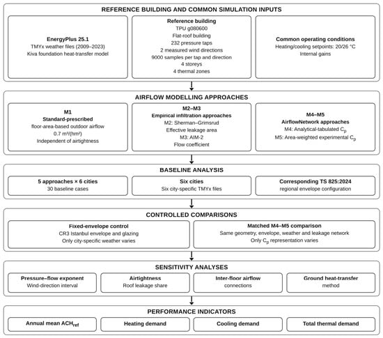
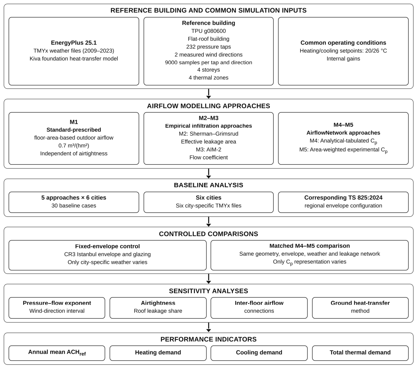
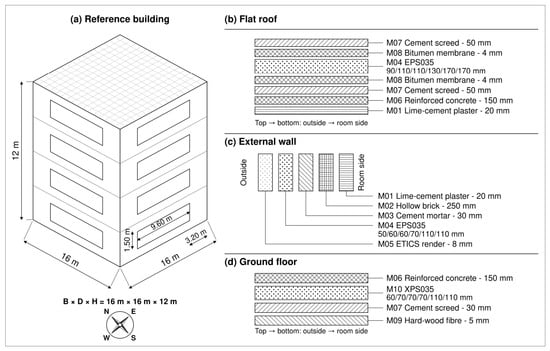
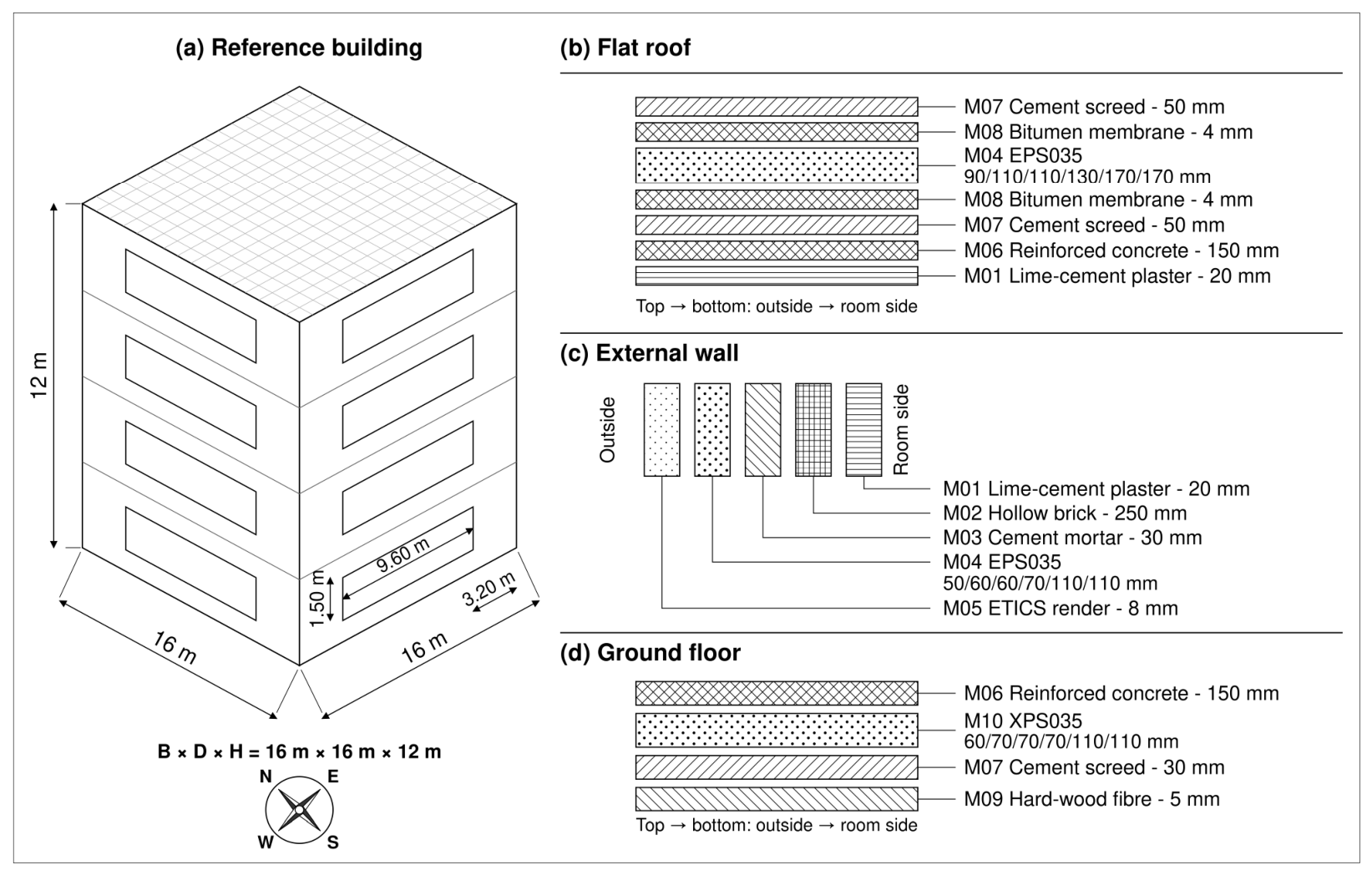
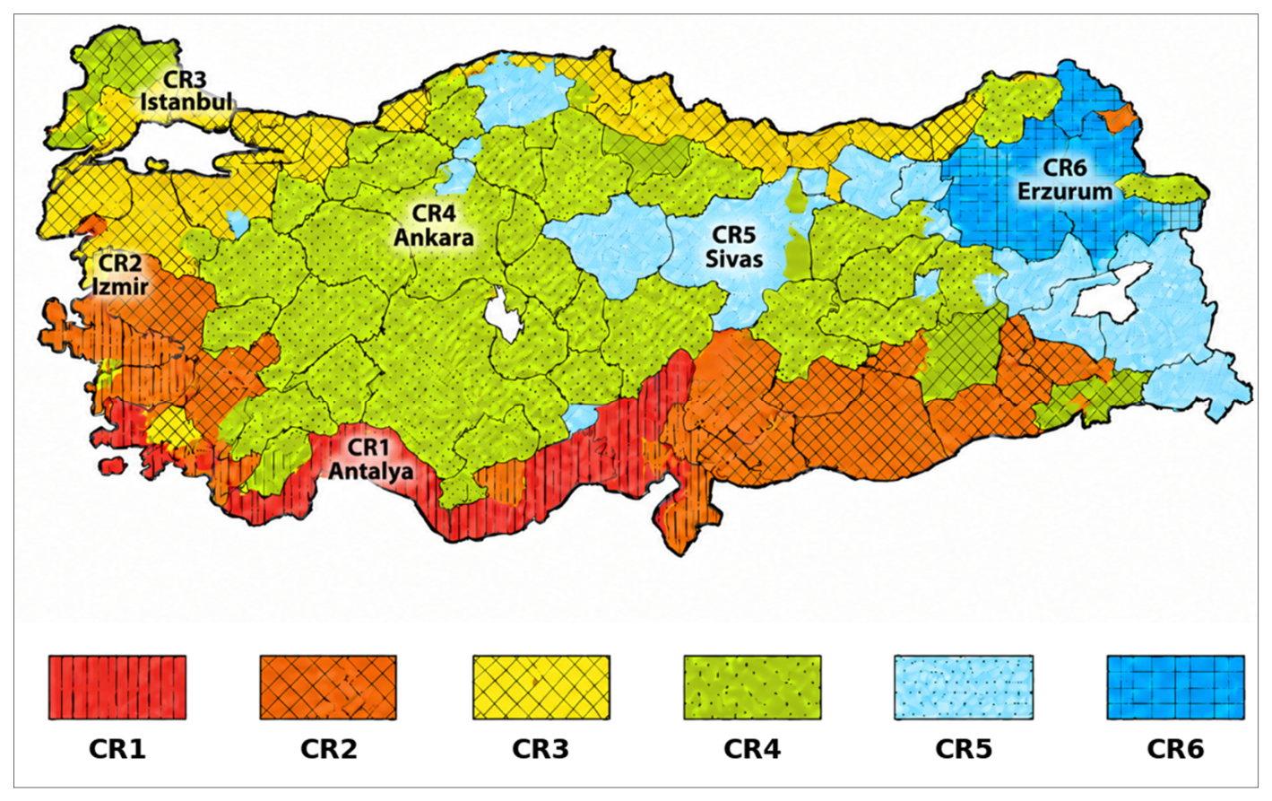
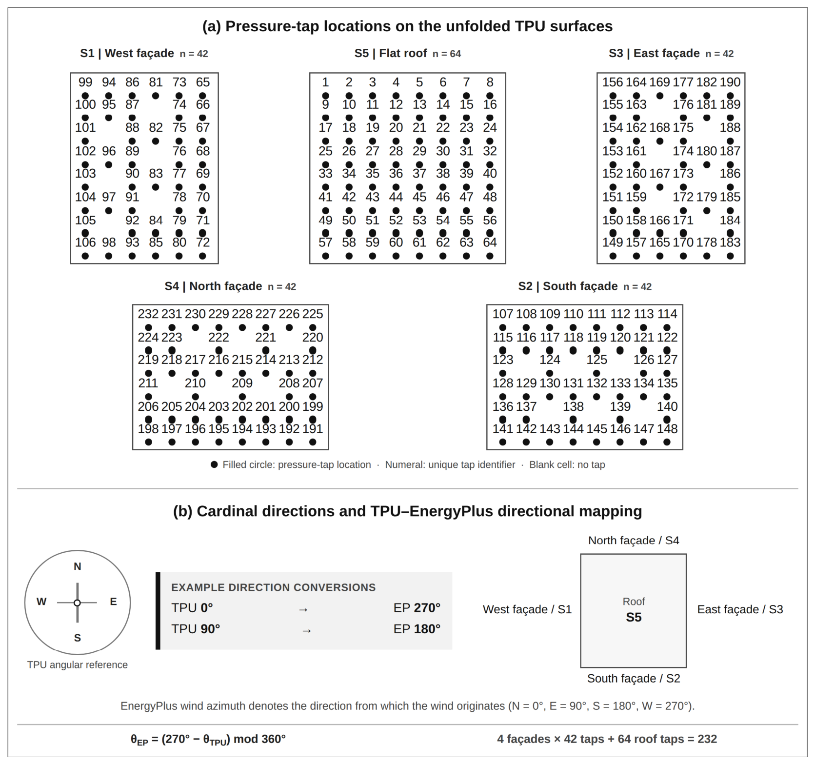
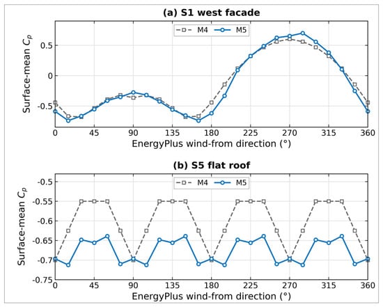
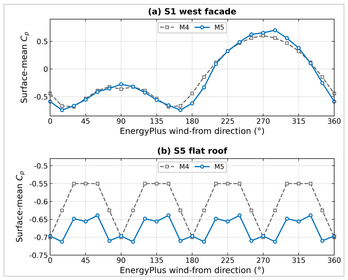
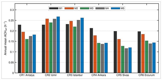
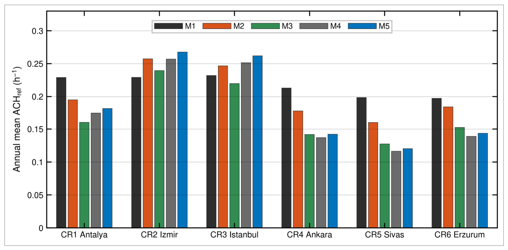
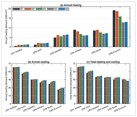
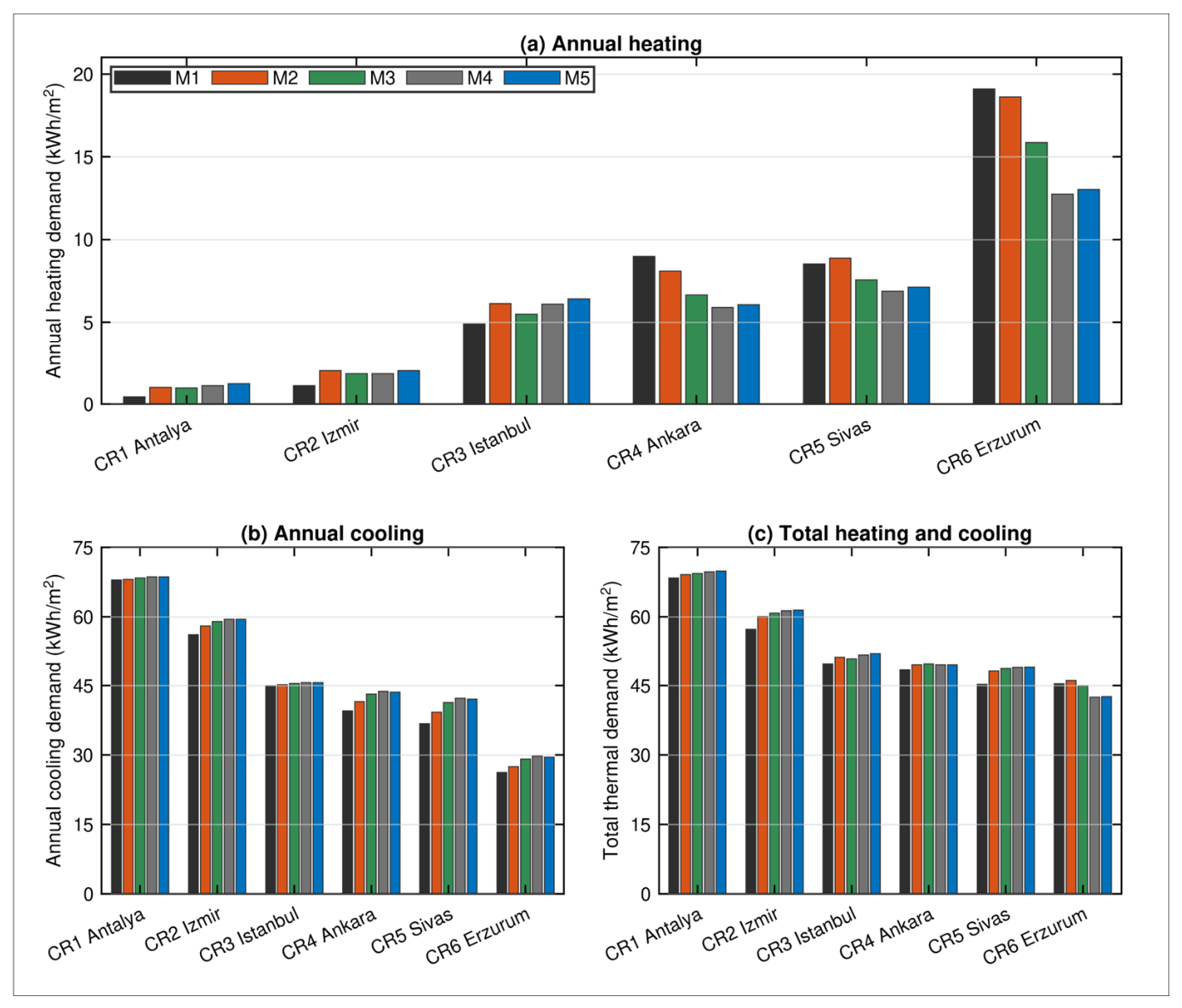
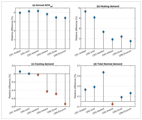
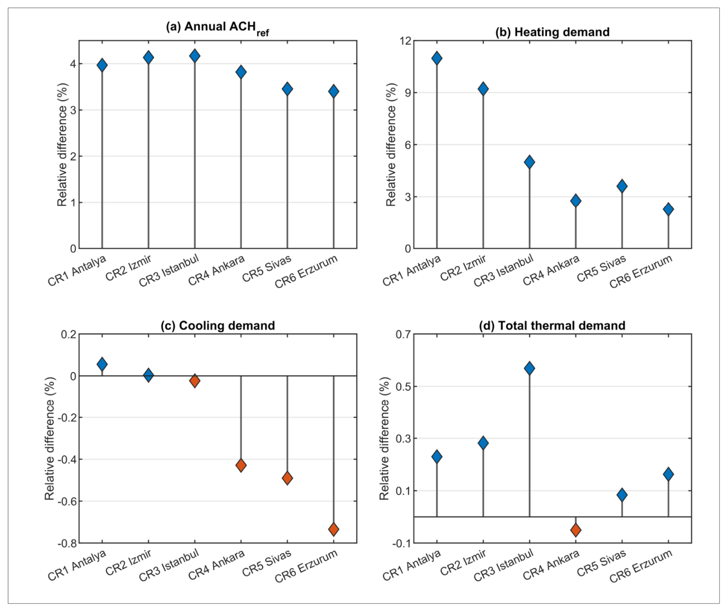
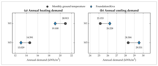
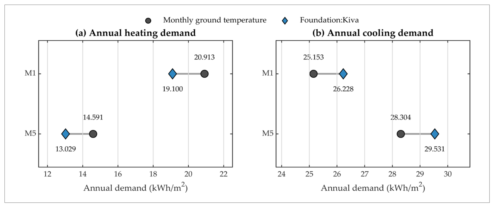
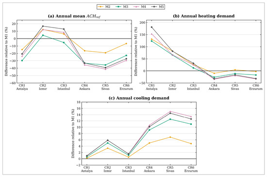
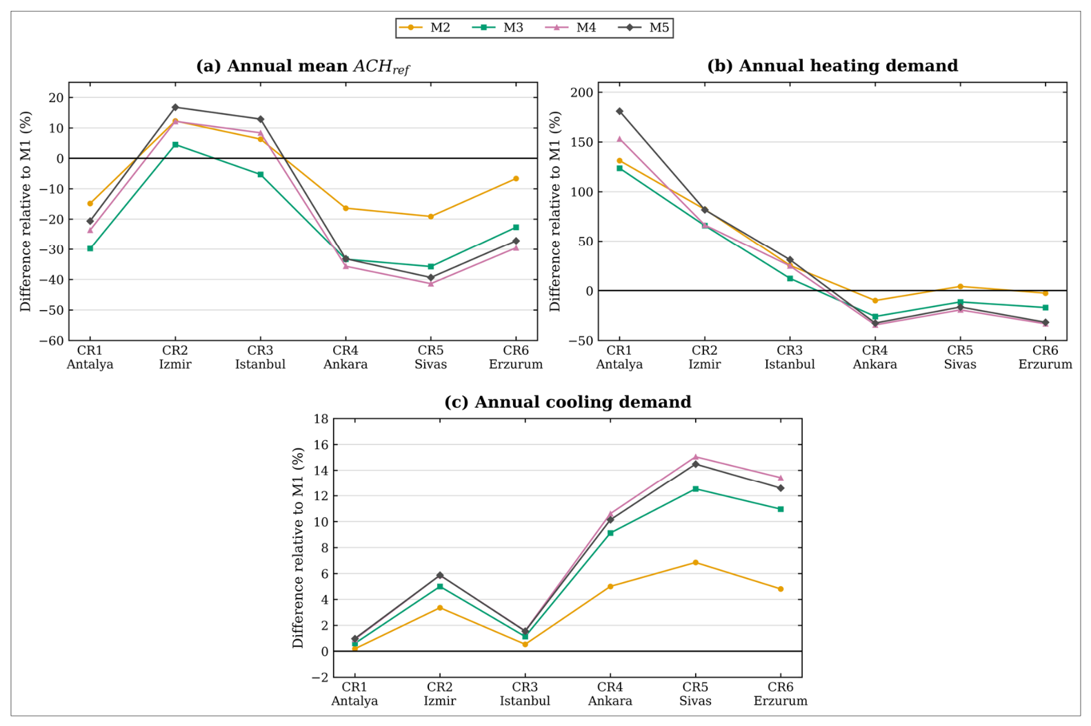

Disclaimer/Publisher’s Note: The statements, opinions and data contained in all publications are solely those of the individual author(s) and contributor(s) and not of MDPI and/or the editor(s). MDPI and/or the editor(s) disclaim responsibility for any injury to people or property resulting from any ideas, methods, instructions or products referred to in the content. |
© 2026 by the author. Licensee MDPI, Basel, Switzerland. This article is an open access article distributed under the terms and conditions of the Creative Commons Attribution (CC BY) license.