Enhancing Energy Efficiency in DHW System with High-Temperature Heat Pumps in a Student Campus

Abstract

This study explores the potential for enhancing the energy efficiency of the domestic-hot-water (DHW) preparation system in a student campus of the Technical University of Cluj-Napoca, Romania, where DHW accounts for approximately 50 ± 10% of total thermal consumption. The current natural gas boiler system is evaluated alongside two energy-enhancing solutions: high-temperature heat pumps utilizing either CO₂ (R744, transcritical cycle) or propane (R290) as refrigerant, for supply temperature scenarios of 75 °C and 55 °C, combined with rooftop photovoltaic systems. Original mathematical models based on real manufacturers’ data are introduced for the components and heat pumps. Expanding the study to eight international locations, the heat pumps cover the entire DHW demand in the simulated scenario, with the boiler retained only as backup, achieving cost reductions between 2.85% and 71.17%. Furthermore, integrating photovoltaics covers significant solar fractions ranging from 21.02% to 83.82% and reduces CO₂ emissions compared to the baseline level in most of the analyzed locations. Across the analyzed locations, payback periods range from 0.4 to 174.7 years for heat pumps alone and from 1.1 to 22.4 years with photovoltaics. A parametric analysis shows that payback is inversely proportional to the price difference, while its non-linearity is driven by the price ratio relative to the break-even threshold.

1. Introduction

Natural-gas-based domestic-hot-water (DHW) preparation contributes directly to CO₂ emissions: the construction sector accounts for 40% of global CO₂ emissions [1], and natural gas use for 22% [2]. Decoupling DHW systems from natural gas is therefore a viable pathway to reduce gas consumption in the EU, within the broader shift toward renewable energy and supporting financial frameworks [3].

Air-to-water heat pumps combined with heat storage are an efficient alternative for DHW preparation [4,5]. Among refrigerants, CO₂ (R744) is a natural, non-flammable, non-toxic option with zero ozone-depletion potential and very low global warming potential, and it is gaining interest for its compatibility with circular-economy goals [6,7]. Propane (R290) offers a negligible global warming impact and competitive SCOP but requires strict safety protocols due to its flammability [8]; its low vapor density reduces system capacity, partly offset by high latent heat of vaporization, and requires larger compressors [9]. High-temperature heat pumps typically supply water at 60–80 °C, exceptionally up to 90 °C [10]; R290 units can reach 75 °C, but with reduced capacity and SCOP [11]. For heat pumps of identical thermal capacity, R290 generally achieves higher SCOP than R744 [12].

Combining heat pumps with sensible heat storage improves operational flexibility and efficiency; phase-change-material (PCM) storage can reduce tank volume [13], although it improves efficiency by only 5.2% over sensible storage [14]. The storage tank is essential for delivering DHW at the required temperature in large-scale systems [15], and stratification modeling is needed to properly represent the vertical temperature gradient [16].

Heat-pump-based DHW retrofits have been studied across several building types: hospitals coupling a heat pump with existing gas and solar systems [17]; apartment buildings connected to district heating [18]; smart buildings integrating heat pumps with PV to avoid costly electrical storage [19]; and photovoltaic–thermal (PVT) systems, with reported COP values between 2.76 and 6.26 depending on climate and season [20,21]. Air-source heat pumps can viably replace gas boilers when COP exceeds three [22], and heat-pump/storage/PV systems for single-family homes can reach solar shares above 60% [23]. Model validation against real operating data has also been demonstrated for PVT-heat pump systems, including economic and CO₂ assessments [24]. Methodologically, such systems have been analyzed both experimentally [7] and via numerical simulation, using TRNSYS [17,21,22,25,26,27] or Modelica [28].

Economic feasibility is equally central to adoption. Long-term financial effects matter more for buildings with high annual DHW demand than short-period assessments [29]; for dormitories, PV-coupled heat pumps improve energy independence, although systems with storage can show longer paybacks than heat-pump-only systems [30]. Economic and environmental feasibility of high-temperature heat pumps in Europe depends strongly on local energy prices [31], governed primarily by the electricity-to-gas price ratio and CO₂ allowance costs; heat pump deployment accelerates where this ratio is low [32]. Across the EU, this ratio ranges from 1.4 to 4.6, and in the Netherlands (the lowest ratio), heat pump sales are three times higher than in countries with ratios above three, such as Germany, Poland, and Hungary [33].

Despite this body of work, comprehensive studies comparing high-temperature air-to-water heat pumps using CO₂ and propane, for buildings with high DHW consumption, remain scarce.

This study addresses this gap by evaluating the DHW preparation system of the Technical University of Cluj-Napoca’s (TUCN) Marasti student campus, currently served by a natural gas boiler, heat exchanger, and storage tank. The objectives of this work are: (i) to develop and validate simplified daily-resolution models of R744 and R290 high-temperature heat pumps, coupled with a stratified storage tank, for annual DHW simulation; (ii) to compare the technical and economic performance of the CO₂ and propane systems against the existing gas-based baseline, across eight countries with different climates and energy prices, including the potential contribution of a photovoltaic system; and (iii) to derive a general, price-based parametric criterion—separating design parameters from market variables—for assessing the economic viability of the heat pump retrofit and of photovoltaic integration, independent of case-specific values.

2. Material

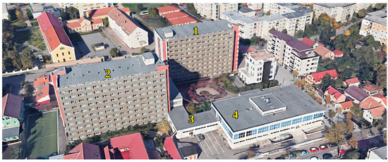
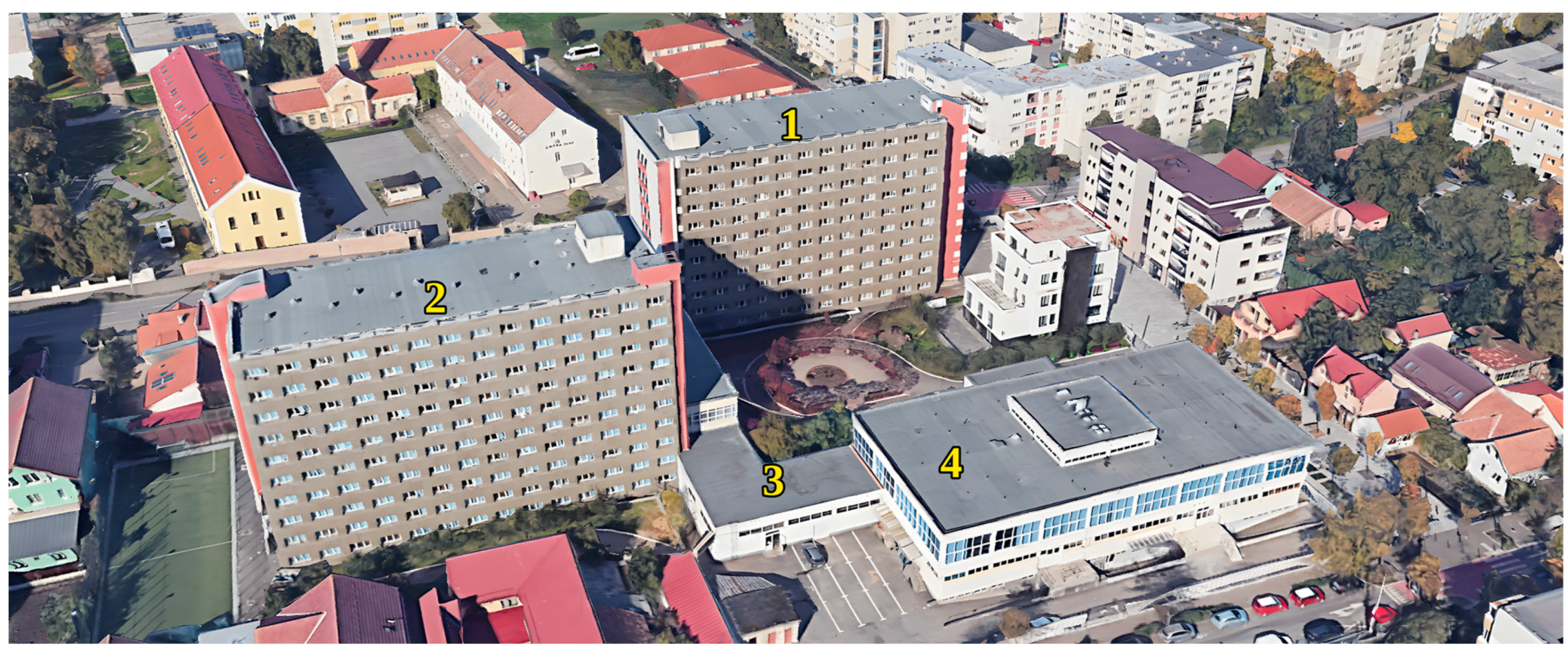
The Marasti student campus of the TUCN is situated in the city of Cluj-Napoca, and Figure 1 presents an image showcasing the constituent buildings of the campus.

Figure 1. The constituent buildings of the campus: 1 and 2—student dormitories; 3—heating plant; 4—cafeteria.

At present, DHW preparation in the student campus is accomplished using a natural gas boiler with a capacity of 1120 kW. The boiler operates at an average efficiency of 80%. DHW is produced via a heat exchanger and stored in a 28 m³ volume storage tank.

Table 1 presents characteristic parameters for the DHW preparation system.

Table 1. The parameters of the DHW preparation and storage system.

Parameter	Value	U.M.
Number of people	1850	-
Quantity of prepared DHW per person in a day	30	l/people/day
Temperature of the prepared DHW	55–60	°C
Temperature of the cold water	10	°C
Temperature on the boiler flow	75	°C
Temperature on the boiler return	55	°C

For this study, the storage tank was modeled using the finite-difference method and discretized into 10 control volumes, numbered from top to bottom. The initial temperature distribution in the tank aligns with the values specified in Table 2.

Table 2. The initial temperature distribution in the tank.

Control Volume	1	2	3	4	5	6	7	8	9	10
Temperature [°C]	60	60	60	60	60	50	40	30	20	10

The study suggests adopting high-temperature heat pumps for DHW preparation, with the necessary electrical energy partially supplied by a dedicated photovoltaic system.

To evaluate the efficiency of the high-temperature air-to-water heat pumps in the DHW preparation system, the behavior of the system was considered in the following locations: Cluj-Napoca, Romania (ROU); Lisboa, Portugal (PRT); Stockholm, Sweden (SWE); Washington, USA (USA); Beijing, China (CHN); Tokyo, Japan (JPN); Paris, France (FRA); Budapest, Hungary (HUN).

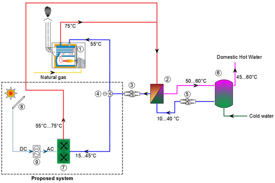
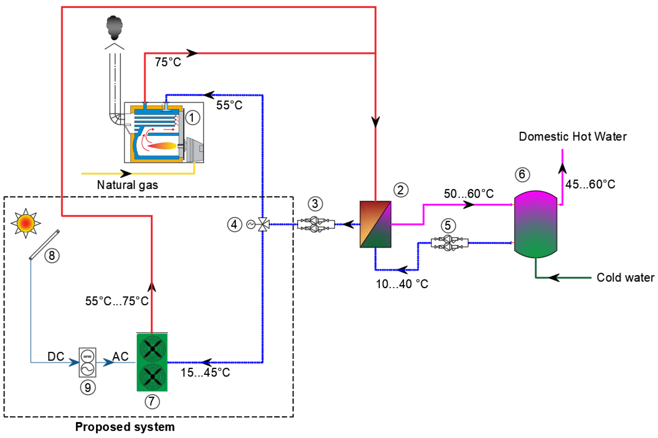
Figure 2 depicts the diagram of the current DHW preparation system and the proposed upgrade.

Figure 2. The diagram of the current and proposed DHW preparation system for the Marasti student campus: 1—natural gas boiler; 2—heat exchanger for DHW; 3, 5—circulation pumps; 4—3-way valve; 6—DHW storage tank; 7—high-temperature heat pump; 8—photovoltaic panels; 9—inverter.

In the existing version, the boiler (1), the primary side of the exchanger (2) and the recirculation pump (2) are denoted as the primary circuit, while the circuit including the secondary side of the heat exchanger (2), the storage tank (6), and recirculation pump (5) is termed the secondary circuit. In the proposed upgrade, the heat pumps (7) are integrated in the primary circuit, while the secondary circuit remains unchanged. The three-way valve (4) allows the switch between the two heat sources.

Two types of air-to-water high-temperature heat pumps and two types of operating thermal regimes were considered. The heat-pump refrigerants and nominal capacities were: R744 (CO₂) at 120 kW and R290 (propane) at 60 kW. The two operating thermal regimes refer to the flow temperatures of 75 °C and 55 °C. Thus, the obtained configurations are designated with the codes below:

−

R744-75: CO₂-based heat pumps operating at a supply temperature of 75 °C.

−

R744-55: CO₂-based heat pumps operating at a supply temperature of 55 °C.

−

R290-75: R290-based heat pumps operating at a supply temperature of 75 °C.

−

R290-55: R290-based heat pumps operating at a supply temperature of 55 °C.

The heat pumps considered are monobloc units installed outdoors, so the refrigerant circuit is factory-sealed and remains outside the building, and only the water circuit enters the technical room. Nevertheless, the flammability of R290 and the high operating pressure of R744 still require safety measures. These include limits on the refrigerant charge, installation clearances and hazardous-zone provisions around the outdoor units, leak detection and pressure protection, in accordance with EN 378 [34] and IEC 60335-2-40 [35]. These aspects are not part of the techno-economic analysis presented here.

The proposed photovoltaic system comprises 250 solar panels (8) with a power rating of 480 Wp and an inverter (9). The reference efficiency of the PV panels is 22.24%, and the aperture area is 2 m². The total aperture area of the system is 500 m².

3. Method

3.1. Climatic Data, Heat Demand and Modeling of the Storage Tank

The heat demand for DHW preparation was determined considering a daily consumption of 30 kg/day/person, the hourly curve of thermal energy consumption for DHW preparation derived from the typical DHW consumption chronogram from [36], and the cold-water temperature variation.

The simulation assumes the design occupancy of 1850 persons during the academic year, with the summer demand reduced to the level derived from the metered gas consumption, as described in Section 4.1.

The average daily temperature of the cold water supplied to buildings (t_cw [°C]) from the public water distribution network was determined using the Burch–Christensen correlation [37]:

$${\mathrm{t}}_{\mathrm{cw}}\left(\mathrm{day}\right)=\left({\mathrm{t}}_{\mathrm{a}}+3.33\right)+\mathrm{k}·{\displaystyle \frac{{∆\mathrm{t}}_{\max }}{2}}·\sin \left[0.986°·\left(\mathrm{day}-15-\mathrm{lag}\right)-90°\right]$$

(1)

k = 0.4 + 0.018 · (t_a − 6.67)

(2)

lag = 35 − 1.8 · (t_a − 6.67)

(3)

where t_a [°C] is the mean annual outdoor air temperature, Δt_max [°C] is the annual air temperature amplitude, and k [-] is the amplitude attenuation ratio and lag [days] is the thermal inertia (time lag).

The climatic data for each location was extracted from the available Typical Meteorological Year (TMY) [38]. The parameters influencing the cold water of the DHW preparation system are presented in Table 3.

Table 3. The parameters influencing the cold water of the DHW preparation system.

Location	ta [°C]	Δtmax [°C]	k [-]	Lag [Days]
ROU	10.0818	20.6322	0.4614	28.8588
PRT	16.2154	10.2099	0.5718	17.8183
SWE	8.1826	18.2773	0.4272	32.2773
USA	14.0537	23.2022	0.5329	21.7094
CHN	12.0730	30.1824	0.4973	25.2747
JPN	15.9240	21.4888	0.5666	18.3428
FRA	11.7998	12.8080	0.4923	25.7664
HUN	12.3746	23.4343	0.5027	24.7318

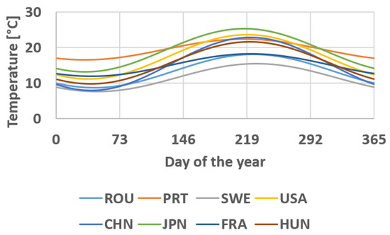
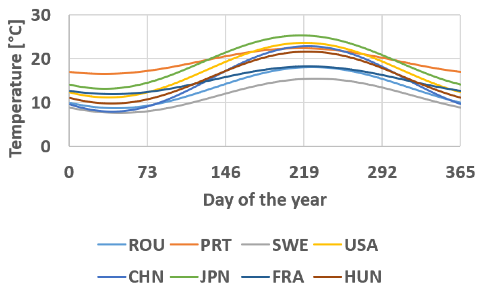
The variation curves of the cold-water temperature of the DHW preparation system for the considered location are presented in Figure 3.

Figure 3. Cold-water supply temperatures for the selected location.

Even if the daily DHW consumption profile and the DHW supply temperature were considered similar for each location, due to the different cold-water temperature variation profile of the DHW preparation system, the thermal load is different for each location.

The simulation of the thermal behavior of the storage tank is carried out through a 1D mathematical model based on the finite-difference method. The principles of the analytical model of the heat storage tank are presented in [39,40,41,42]. The control volumes (1–n), counted from top to bottom, are treated as lumped systems, and the heat transfer between the control volumes is considered unidirectional. For the water in tanks without coils, the conductivity of water was calculated as a function of temperature [43].

The finite-difference modeling approach was developed and validated in detail in earlier work [40,41,44], dedicated specifically to the thermal behavior of stratified storage tanks. The stratified model was validated against results available in the literature for tanks with volumes from 0.75 to 1000 m³, heated by electric boilers, cogeneration-based district heating and solar thermal plants [40], and the seasonal-storage tanks of solar district heating systems were modeled for volumes from 8500 to 22,829 m³, including the preparation of domestic hot water [40,41,44]. The volume of 28 m³ analyzed here lies within the validated range. The present study applies this validated method to a new case rather than re-validating it. The specific 28 m³ tank geometry and stratification behavior analyzed here were not independently validated against measured data. The model considers only heat transfer between control volumes. Thermal losses to the surroundings were not included, as the tank is installed indoors, in a technical room where the ambient temperature remains relatively constant throughout the year. Under these conditions, such losses are expected to be limited and largely independent of outdoor weather or season. This is noted as a simplifying assumption.

3.2. Modeling the Thermal Behavior of Heat Pumps

The purpose of modeling the thermal behavior of heat pumps is to determine the provided thermal power and the COP, both depending on external operating conditions. These conditions are characterized by the outdoor temperature and the return temperature of the hot-water circuit for R744, whereas for R290, they depend on the outdoor and supply temperatures. The electrical power needed by heat pumps is influenced by both the generated thermal power and the COP. The equations were determined for real operating conditions tested by manufacturers.

For the variation in the COP depending on the outdoor temperature (t_ext [°C]), the following equation is proposed:

$$\mathrm{COP}=\mathrm{a}·{{\mathrm{t}}_{\mathrm{ext}}}^2+\mathrm{b}·{\mathrm{t}}_{\mathrm{ext}}+\mathrm{c}$$

(4)

For R744, the equations are based on manufacturer data for outdoor temperatures between −15 °C and +15 °C. Outside this interval the COP (respectively the thermal power) is kept equal to its value at the nearest boundary and is not extrapolated. In the Typical Meteorological Year used for Cluj-Napoca, the outdoor temperature is below −15 °C for only 24 h per year (0.27% of the time), with a minimum of −16.84 °C. The coefficients a, b and c depend on the return temperature of the heat pumps (t_r [°C]) as follows:

$$\mathrm{a}={\mathrm{a}}_1·{{\mathrm{t}}_{\mathrm{r}}}^2+{\mathrm{a}}_2·{\mathrm{t}}_{\mathrm{r}}+{\mathrm{a}}_3$$

(5)

$$\mathrm{b}={\mathrm{b}}_1·{{\mathrm{t}}_{\mathrm{r}}}^2+{\mathrm{b}}_2·{\mathrm{t}}_{\mathrm{r}}+{\mathrm{b}}_3$$

(6)

$$\mathrm{c}={\mathrm{c}}_1·{{\mathrm{t}}_{\mathrm{r}}}^2+{\mathrm{c}}_2·{\mathrm{t}}_{\mathrm{r}}+{\mathrm{c}}_3$$

(7)

The valid range of these equations is t_r = (10–50) °C.

For R290, the equation is valid within the range t_ext = (−20–45) °C. The coefficients a, b and c depend on the supply temperature of the heat pumps (t_s [°C]) as follows:

$$\mathrm{a}={\mathrm{a}}_1·{{\mathrm{t}}_{\mathrm{s}}}^2+{\mathrm{a}}_2·{\mathrm{t}}_{\mathrm{s}}+{\mathrm{a}}_3$$

(8)

$$\mathrm{b}={\mathrm{b}}_1·{{\mathrm{t}}_{\mathrm{s}}}^2+{\mathrm{b}}_2·{\mathrm{t}}_{\mathrm{s}}+{\mathrm{b}}_3$$

(9)

$$\mathrm{c}={\mathrm{c}}_1·{{\mathrm{t}}_{\mathrm{s}}}^2+{\mathrm{c}}_2·{\mathrm{t}}_{\mathrm{s}}+{\mathrm{c}}_3$$

(10)

The coefficient values a₁, a₂, a₃, b₁, b₂, b₃, c₁, c₂ and c₃ are presented in Table 4.

Table 4. The coefficient values a₁, a₂, a₃, b₁, b₂, b₃, c₁, c₂ and c_3.

Coefficient	R744				R290
	ts = 75 °C		ts = 55 °C
	Tr ≤ 25 °C	Tr > 25 °C	Tr ≤ 25 °C	Tr > 25 °C
a1	0	−0.000001123	0	0.000001097	0.0000006
a2	−0.000035455	0.000046363	−0.000033415	−0.000137425	−0.0000900
a3	0.00226157	0.000132646	0.00243379	0.00392832	0.0044000
b1	0	−0.000005206	0	0.000006652	0.0000400
b2	−0.00220284	−0.000168172	−0.00167149	−0.00157051	−0.0064000
b3	0.124829	0.0507162	0.124737	0.093358	0.3124000
c1	0	−0.00149506	0	−0.0015221	0.0013000
c2	−0.0520637	0.101547	−0.0412863	0.0981793	−0.2006000
c3	3.83634	0.296366	3.87474	0.664857	9.8091000

To reduce the deviations between the correlation and the manufacturer data, the coefficients a, b and c of the R744 heat pump were re-fitted separately for two return-temperature ranges, t_r ≤ 25 °C and t_r > 25 °C. For t_r ≤ 25 °C the quadratic term vanishes (a₁ = b₁ = c₁ = 0), so Equations (5)–(7) reduce to a linear function of t_r; for t_r > 25 °C the full quadratic form of Equations (5)–(7) is retained. Both coefficient sets are given in Table 4.

Table 5 and Table 6 present the relative calculation deviations for the COP of R744 and R290, respectively, comparing the values derived from the proposed equations with manufacturer data.

Table 5. The values of the relative calculation deviations for the COP of R744.

ts	tr [°C]	text [°C]
[°C]		−15	−10	−5	0	5	10	15
75	10	−0.13%	0.20%	0.07%	−0.04%	−0.13%	−0.20%	0.23%
	20	−0.17%	0.30%	0.02%	−0.11%	−0.13%	−0.08%	0.17%
	30	−0.01%	0.00%	0.03%	0.02%	−0.02%	−0.07%	0.06%
	40	0.14%	−0.19%	−0.09%	0.01%	0.13%	0.24%	−0.22%
	50	−0.01%	−0.06%	0.09%	0.09%	−0.03%	−0.25%	0.15%
55	10	−0.12%	0.19%	0.06%	−0.04%	−0.11%	−0.16%	0.20%
	20	−0.15%	0.25%	0.03%	−0.09%	−0.12%	−0.10%	0.17%
	30	−0.05%	0.08%	0.01%	−0.02%	−0.04%	−0.04%	0.06%
	40	−0.05%	0.09%	0.00%	−0.03%	−0.03%	−0.00%	0.03%
	50	−0.02%	0.04%	0.01%	−0.01%	−0.02%	−0.03%	0.04%

Table 6. The values of the relative calculation deviations for the COP of R290.

ts [°C]		text [°C]
	−20	−15	−10	−5	0	5	10	15	20
35	0.04%	0.57%	0.67%	0.48%	0.11%	−0.34%	−0.82%	−1.31%	−1.79%
45	0.58%	1.36%	1.40%	0.95%	0.21%	−0.68%	−1.63%	−2.59%	−3.51%
55	1.53%	1.83%	1.13%	−0.22%	−1.93%	−3.83%	−5.76%	−7.67%	−9.48%
65	3.57%	7.53%	7.18%	5.64%	2.05%	−1.03%	−2.55%	−3.19%	−6.22%

The maximum deviations for the COP from the manufacturer-provided values are 0.30% for R744 and 9.48% for R290. The largest COP deviations for R290 occur at the higher supply temperatures: up to 9.48% for t_s = 55 °C and t_ext = 20 °C and up to 7.53% for t_s = 65 °C and t_ext = −15 °C, while for t_s = 35 and 45 °C they remain below 3.6%.

For the variation in thermal power ($\dot{\mathrm{Q}}$ [kW]) as a function of external temperature (t_ext [°C]) the proposed equation is

$${\dot{\mathrm{Q}}}_{\mathrm{h}}=\mathrm{m}·{{\mathrm{t}}_{\mathrm{ext}}}^2+\mathrm{n}·{\mathrm{t}}_{\mathrm{ext}}+\mathrm{p}$$

(11)

For R744, the equations are based on manufacturer data for outdoor temperatures between −15 °C and +15 °C. Outside this interval the value of $\dot{\mathrm{Q}}$ is kept equal to its value at the nearest boundary and is not extrapolated. The coefficients m, n and p depend on the return temperature of the heat pumps (t_r [°C]) as follows:

$$\mathrm{m}={\mathrm{m}}_1·{{\mathrm{t}}_{\mathrm{r}}}^2+{\mathrm{m}}_2·{\mathrm{t}}_{\mathrm{r}}+{\mathrm{m}}_3$$

(12)

$$\mathrm{n}={\mathrm{n}}_1·{{\mathrm{t}}_{\mathrm{r}}}^2+{\mathrm{n}}_2·{\mathrm{t}}_{\mathrm{r}}+{\mathrm{n}}_3$$

(13)

$$\mathrm{p}={\mathrm{p}}_1·{{\mathrm{t}}_{\mathrm{r}}}^2+{\mathrm{p}}_2·{\mathrm{t}}_{\mathrm{r}}+{\mathrm{p}}_3$$

(14)

The valid range of these equations is t_r = (10–50) °C.

For R290, the equation is valid within the range t_ext = (−20–45) °C. The coefficients m, n and p depend on the supply temperature of the heat pumps (t_s [°C]) as follows:

$$\mathrm{m}={\mathrm{m}}_1·{{\mathrm{t}}_{\mathrm{s}}}^2+{\mathrm{m}}_2·{\mathrm{t}}_{\mathrm{s}}+{\mathrm{m}}_3$$

(15)

$$\mathrm{n}={\mathrm{n}}_1·{{\mathrm{t}}_{\mathrm{s}}}^2+{\mathrm{n}}_2·{\mathrm{t}}_{\mathrm{s}}+{\mathrm{n}}_3$$

(16)

$$\mathrm{p}={\mathrm{p}}_1·{{\mathrm{t}}_{\mathrm{s}}}^2+{\mathrm{p}}_2·{\mathrm{t}}_s+{\mathrm{p}}_3$$

(17)

The values of the coefficients m₁, m₂, m₃, n₁, n₂, n₃, p₁, p₂ and p₃ are presented in Table 7.

Table 7. The coefficient values m₁, m₂, m₃, n₁, n₂, n₃, p₁, p₂ and p_3.

Coefficient	R744				R290
	ts = 75 °C		ts = 55 °C
	Tr ≤ 25 °C	Tr > 25 °C	Tr ≤ 25 °C	Tr > 25 °C
m1	0	0.000074251	0	−0.000015662	−0.00001
m2	−0.00059739	−0.00729988	−0.00047202	0.00013037	0.00050
m3	0.02184445	0.15520282	0.02226541	0.01289873	0.01750
n1	0	−0.0005594	0	0.00119995	−0.00008
n2	−0.05589491	0.05396563	−0.04429139	−0.08169121	−0.00810
n3	3.18530443	0.64114906	3.22834104	3.19218496	1.84740
p1	0	−0.04079605	0	−0.01018889	0.00150
p2	−1.60554006	2.63273525	−1.27176283	0.38061365	−0.30410
p3	118.35885042	37.473549	119.58906266	79.2461065	57.71200

In the same way, the coefficients m, n and p of the R744 heat pump were re-fitted separately for t_r ≤ 25 °C and t_r > 25 °C. For t_r ≤ 25 °C the quadratic term vanishes (m₁ = n₁ = p₁ = 0), so Equations (12)–(14) reduce to a linear function of t_r; for t_r > 25 °C the full quadratic form of Equations (12)–(14) is retained. Both coefficient sets are given in Table 7.

Since the COP and thermal power equations (Equations (4) and (11)) are derived from real operating-condition data tested by the manufacturers, rather than idealized steady-state values, the effects of defrosting are expected to be at least partly reflected in the fitted curves to an extent that cannot be fully confirmed from the available data. No separate defrost cycle or backup-heating strategy was explicitly modeled at the system level, and the possible use of the gas boiler as temporary support, described in Section 4.2, was not quantified; these aspects are noted here as limitations.

Table 8 and Table 9 present the relative calculation deviations for the thermal power produced by the heat pumps of R744 and R290, respectively, comparing the values derived from the proposed equations with manufacturer data.

Table 8. The values of the relative calculation deviations for the thermal power produced by the heat pumps of R744.

ts	tr [°C]	text [°C]
[°C]		−15	−10	−5	0	5	10	15
75	10	0.15%	−0.00%	−0.00%	−0.00%	−0.00%	−0.00%	−0.06%
	20	0.17%	0.00%	0.00%	−0.00%	0.00%	0.00%	−0.08%
	30	0.23%	−0.01%	−0.00%	−0.00%	−0.00%	−0.00%	−0.08%
	40	−2.28%	−0.00%	−0.00%	−0.00%	−0.00%	−0.00%	0.77%
	50	2.33%	−0.01%	−0.00%	−0.00%	−0.00%	−0.00%	−0.41%
55	10	0.14%	−0.01%	−0.00%	−0.00%	−0.00%	−0.00%	−0.06%
	20	0.15%	−0.00%	−0.00%	0.00%	−0.00%	−0.00%	−0.07%
	30	0.44%	−0.00%	0.00%	0.00%	0.00%	−0.00%	−0.14%
	40	−0.81%	0.01%	0.00%	−0.00%	0.00%	0.00%	0.24%
	50	2.06%	0.01%	0.00%	0.00%	0.00%	0.00%	−0.38%

Table 9. The values of the relative calculation deviations for the thermal power produced by the heat pumps of R290.

ts [°C]		text [°C]
	−20	−15	−10	−5	0	5	10	15	20
35	0.15%	0.18%	0.17%	0.12%	0.06%	−0.01%	−0.08%	−0.15%	−0.22%
45	0.19%	0.19%	−0.25%	−0.49%	−0.57%	−0.54%	−0.43%	−0.29%	−0.13%
55	0.93%	0.59%	0.63%	0.04%	−0.29%	−0.43%	−0.44%	−0.35%	−0.20%
65	2.31%	0.69%	0.76%	−0.26%	−0.69%	0.36%	−0.03%	−0.33%	−0.51%

The maximum deviations for the thermal power from the manufacturer-provided values are 2.33% for R744 and 2.31% for R290.

Across the full set of 212 tested operating points (106 for COP, 106 for thermal power), the mean absolute percentage deviation (MAPD) and root-mean-square deviation (RMSD) from manufacturer data are 0.92%/2.07% for COP and 0.24%/0.51% for thermal power. These deviations were computed against the same manufacturer dataset used to fit the regression coefficients (Table 4 and Table 7), and an independent validation dataset was not available.

For the thermal behavior of the storage tank, a 1 min time step was considered, because of the relatively high-speed temperature variations.

Since such a small time step is impractical for simulations covering the entire year, six intervals of 5 consecutive days each were selected to determine the average COP and delivered thermal power of the HP variations as a function of the daily average temperature. These intervals were chosen as calibration points covering the full range of operating conditions of the heat pumps, and not as a representative sample of typical periods. Thus, a 1-day time step could be used for the whole year simulation.

For these 5-day intervals, the maximum and minimum temperatures, range of daily average temperature variation, and the average of the daily average temperatures (referred to as the characteristic daily average temperature) were determined. These values are presented in Table 10.

Table 10. The characteristics of the curves depicting the variation in external temperatures.

Interval Code	Maximum Temperature [°C]	Minimum Temperature [°C]	Daily Average Temperature [°C]	Characteristic Daily Average Temperature [°C]
Int1	36.4	17.2	26.4–28.1	27.25
Int2	25.3	11.9	17.9–20.2	19.05
Int3	16.1	4.9	10.3–12.7	11.5
Int4	4.8	−3.6	0.9–2.1	1.5
Int5	−1.7	−16.8	−7.2–−11.3	−9.25
Int6	−3.3	−16.8	−7.6–−11.3	−9.45

For each of these intervals, the following parameters were determined:

-

Variation curves of temperatures in the layers of the storage tank;

-

Variation curves of COP as a function of external temperature and return temperature (represented by the temperature in the lower layer of the tank) for R744, and as a function of both external and supply temperatures for R290.

-

Variation curves of thermal powers: at the consumer, introduced and extracted from the tank;

-

Variation curves of the electrical power consumed by the heat pumps;

-

Variation curves of the flow rates in each circuit.

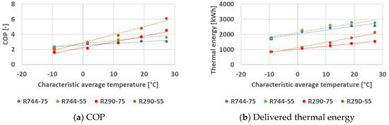
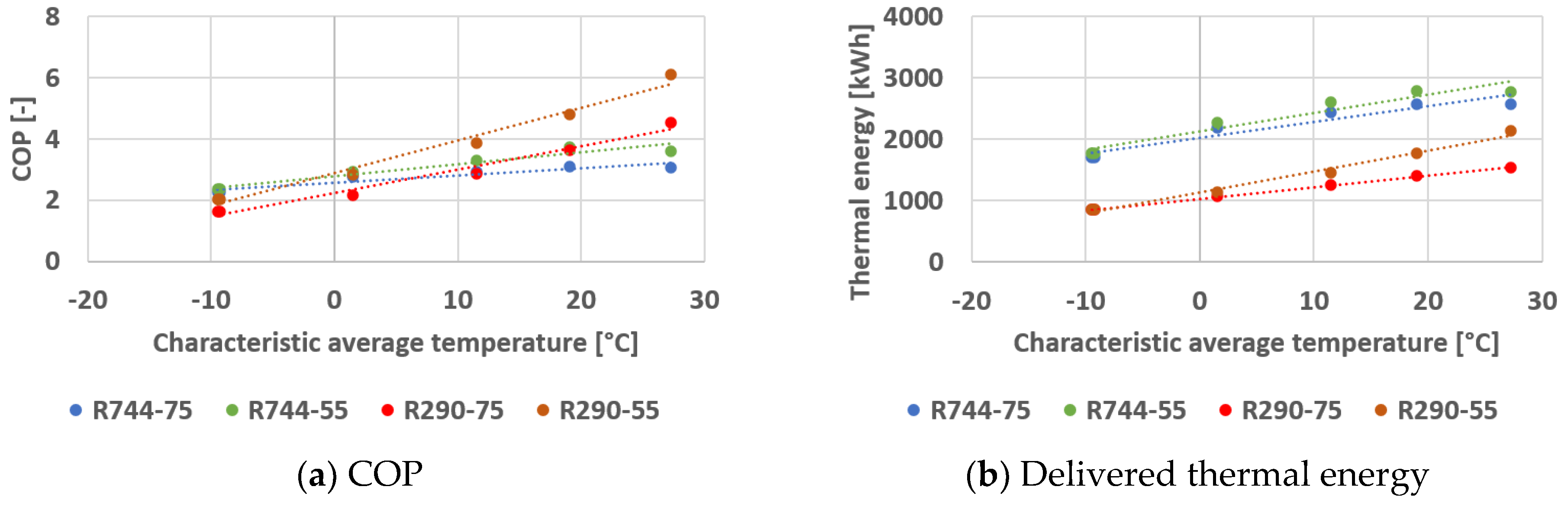
The COP values, along with the thermal power produced by the heat pumps, were continuously determined for each 5-day interval using the proposed equations with a time step of 1 min. Subsequently, the daily average values for COP and the daily delivered thermal energy of each heat pump were determined based on the characteristic daily average temperature for each considered interval. The variation curves for these two quantities are presented in Figure 4.

Figure 4. The daily average COP variation curve and the daily average variation curve of delivered thermal energy.

In the next stage, an equation was proposed for calculating the daily average values of COP and the daily thermal energy produced by each heat pump.

The proposed equation for calculating the daily average COP variation (COP_da [-]) as a function of the characteristic daily average temperature t_da [°C] is

COP_da = r · t_da + s

(18)

The proposed equation for calculating the daily average variation in delivered thermal energy (Q_da [kWh]) as a function of the characteristic daily average temperature is

Q_da = y · t_da + z

(19)

The coefficient values for Equations (18) and (19) are presented in Table 11.

Table 11. The coefficient values for Equations (18) and (19).

Coefficients	r	s	y	z
Values for R744-75	0.0239	2.5653	25.823	2018.8
Values for R744-55	0.0388	2.7831	30.247	2125.7
Values for R290-75	0.0759	2.2313	19.031	1028.1
Values for R290-55	0.1063	2.8912	34.100	1135.3

The six intervals therefore cover the full range of operating conditions of the heat pumps. The performance of the heat pumps depends only on the outdoor temperature, on the return temperature (R744) and on the supply temperature (R290), and these parameters are included in the mathematical models (Equations (4)–(17)). As a consequence, Equations (18) and (19) do not depend on the location. The location only determines the outdoor temperature, which is taken from the climatic data. At the study location, the daily average temperature of 363 of the 365 days lies within the range of daily averages of the six intervals (−11.3 to 28.1 °C). The two coldest days, with a minimum of −12.55 °C, are up to 1.3 K below this range, where Equations (18) and (19) are slightly extrapolated.

With the proposed equations, variations in average daily COP and daily thermal energy produced by the heat pumps were determined for the one-year interval, with a time step of 1 day.

3.3. The Calculation of the Electrical Efficiency of Photovoltaic Collectors

The electrical efficiency of photovoltaic collectors (η_PV [%]) is determined by the following relation [45]:

$${\mathsf{\eta }}_{\mathrm{PV}}={\mathsf{\eta }}_{\mathrm{Tref}}\left\{1-{\mathsf{\beta }}_{\mathrm{ref}}\left[{\mathrm{T}}_{\mathrm{a}}-{\mathrm{T}}_{\mathrm{ref}}+\left({\mathrm{T}}_{\mathrm{NOCT}}-{\mathrm{T}}_{\mathrm{aNOCT}}\right){\displaystyle \frac{{\mathrm{I}}_{\mathrm{gt}}}{{\mathrm{I}}_{\mathrm{gNOCT}}}}\right]\right\}$$

(20)

where

-

T_NOCT [K]/ t_NOCT [°C] is the normal operating collector temperature under the following test conditions: air temperature, t_aNOCT = 20 °C/ T_aNOCT = 293 K; global solar radiation intensity, I_gNOCT = 800 W/m²; wind speed w = 1 m/s;

-

T_aNOCT = 293 K/ t_aNOCT = 20 °C is the air temperature under test conditions used to determine the normal operating collector temperature (t_NOCT [°C]/ T_NOCT [K]);

-

I_gNOCT = 800 W/m² is the value of global solar radiation intensity under test conditions used to determine the normal operating collector temperature (t_NOCT [°C]/ T_NOCT [K]).

3.4. Economic Analysis

To evaluate the economic feasibility of the investment, this study was extended to seven additional countries, aiming to highlight the viability of the technical solutions in the context of varying local energy prices. Table 12 presents the energy prices used in this research.

Table 12. The energy prices used in this research.

Country	R	NGP	EP	PVP	Ref.
[-]	[-]	[€/MWh]	[€/MWh]	[€/kWp]	[-]
ROU	0.29	55.9	191.8	1000	[46,47,48]
PRT	0.53	126.5	239.0	900	[46,47,48]
SWE	0.80	212.8	265.4	1200	[46,47,48]
USA	0.23	44.0	190.0	1400	[48,49]
CHN	0.51	46.0	90.0	700	[48,49]
JPN	0.27	68.0	250.0	1500	[48,49]
FRA	0.49	129.8	266.4	1200	[46,47,48]
HUN	0.30	30.7	104.0	1000	[46,47,48]

Notations: R—ratio between gas price/electricity price; NGP—natural gas price; EP—electricity price; PVP—photovoltaic system price.

The purchase price of the heat pumps for all countries except China was set at €82,000 for R744 units and €19,000 for R290 units, based on the price list of an EU heat pump provider. For China, the purchase prices of the heat pumps were assumed to be 60% of the values mentioned above, respectively €49,200 for R744 units and €11,400 for R290 units. This investment reflects equipment purchase cost only; installation, electrical and piping upgrades, and maintenance are not included.

The annual savings in the case of using heat pumps were determined as the difference between the cost of natural gas consumption by the boiler and the cost of electrical energy required for the heat pumps.

The payback period (PB [year]) for each scenario was calculated using the following relationship:

PB = η · Π · (1 − R)/(R − R_be)

(21)

where η [-] is seasonal efficiency of the replaced boiler, Π [-] is dimensionless investment index, R [-] is ratio between gas price/electricity price, and R_be [-] is break-even price ratio, with an option without PV.

Dimensionless investment index is

$$\mathsf{\Pi }={\displaystyle \frac{\mathrm{I}}{\mathrm{Q}·\mathrm{D}}}$$

(22)

where D [€/MWh] is the difference between electricity price and gas price, I [€] is total investment in the new solution, and Q [MWh/yr] is annual useful heat demand for DHW preparation.

Equation (21) is formulated through a set of variables that entirely separates design-related parameters from market-driven ones. The entire effect of the investment and of the heat demand is concentrated in the factor Π, and the entire effect of prices in the factor (1 − R)/(R − R_be), which does not depend on the size of the installation. Equation (21) has an immediate methodological consequence: the preliminary assessment of a project does not require a complete balance. The heat demand and the investment enter only afterwards, as a scaling factor.

The payback period is calculated as a simple (undiscounted) metric; discount rate, inflation, and long-term energy price escalation are not included. Operating expenses are limited to energy costs, and component replacement—including periodic PV inverter replacement, typically required within the system’s operational lifetime—is not accounted for.

4. Results and Discussion

4.1. Existing DHW System

Two operating scenarios for the gas boiler were investigated, each considering different thermal powers:

-

Nominal power of the boiler, P = 1120 kW.

-

Reduced power scenario: P = 300 kW, which represents 73% of the nominal power.

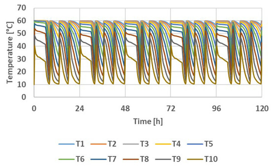
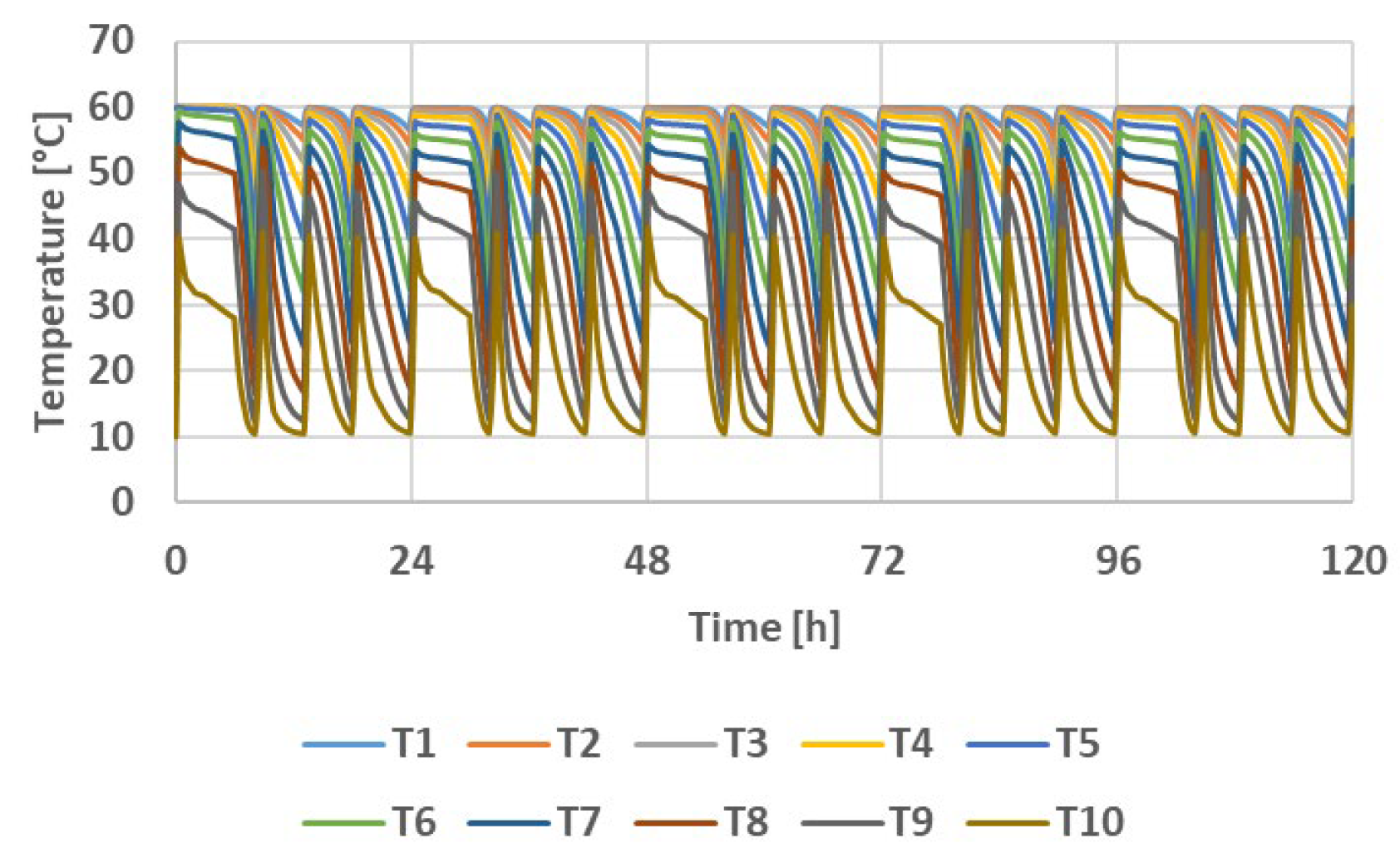
The simulations assume a constant cold-water supply temperature of 10 °C. Figure 5 illustrates the hourly variation in the temperature distribution in the layers of the storage tank over a period of 5 consecutive days for the boiler operating at nominal power.

Figure 5. The hourly variation in temperature distribution in the layers of the storage tank over 5 days for the boiler at nominal power.

At nominal power, the boiler initiates four daily short startup cycles to meet the heat demand for DHW preparation. The storage tank contributes to energy savings and ensures peak consumption. The duration of each startup period is approximately (30–50) minutes. If the thermal power of the boiler is 300 kW, it starts twice in 24 h, and the duration of the tank charging processes increases by (7–8) times, or (230–400) minutes compared to the durations corresponding to the nominal power of 1120 kW.

When the boiler is operating at its nominal power, the thermal power entering the tank varies between (0–1120) kW, and the thermal power leaving the tank varies between (0–408) kW. The thermal power entering the tank varies between (0–300) kW in the reduced power scenario, and the thermal power exiting the tank varies between (0–406) kW.

The system boundary adopted for the existing installation includes the gas boiler and the primary-side heat exchanger. Circulation-pump electricity, distribution losses and standby losses of the storage system were excluded, as the analysis targets the primary-energy carrier at the heat generation point. The boiler efficiency of 80% is a global parameter, defined at the annual level [50,51], and it is used only to convert the useful heat into the natural gas consumption of the baseline, which enters the economic comparison. It is treated as constant, so the additional losses associated with short-cycling and part-load operation are not captured. This is a conservative simplification, since accounting for real part-load losses would only improve the relative economics of the heat-pump alternative.

To check the demand model, the monthly natural gas energy calculated for the existing boiler (useful heat divided by η = 0.80) was compared with the metered gas consumption of the campus for June–September, the only months for which measurements were available and in which space heating is not operated. In June, when the campus is still occupied, the calculated value (100.7 MWh) agrees with the measured one (99.9 MWh) within 0.8%, supporting the adopted consumption of 30 L/person/day and the cold-water temperature model. In July, August and September the measured consumption (58.7, 33.8 and 34.6 MWh) is 41%, 66% and 64% lower than calculated, reflecting the student holidays, when the dormitories are largely unoccupied; the model, which assumes constant full occupancy, does not reproduce this effect. The calculated July–September values were therefore replaced with the measured ones, which reduces the annual gas-equivalent demand from 1296 to 1128 MWh (−13%), corresponding to 902 MWh of useful heat. This occupancy-adjusted demand is used in all the simulations presented in the following sections. Measured data were not available for the other months or for the hourly profile, which is taken from [36] and is therefore not validated against campus data. This is noted as a limitation.

It is noteworthy that, despite the current DHW preparation system being equipped with a 1120 kW boiler, the maximum thermal power required at the consumer is only slightly more than 400 kW. Due to the presence of the heat storage system, the system can operate efficiently even with a boiler delivering only 300 kW.

It can be observed that in the current situation, the boiler is oversized, probably because at the time of its installation, there was no storage tank, and the boiler was selected to be capable of covering consumption peaks, estimated to be much higher.

The maximum flow rates are 13.4 kg/s in the primary circuit, 13.3 kg/s in the secondary circuit and 1.9 kg/s in the DHW consumption circuit for the boiler at nominal power scenario and 3.6 kg/s, in both primary and secondary circuits and 1.9 kg/s in the DHW consumption circuit for the boiler in the reduced power scenario.

4.2. The DHW Preparation System with Heat Pumps in Cluj-Napoca

The operation of the DHW preparation system with high-temperature heat pumps, serving as sources of thermal energy has been analyzed over periods of 5 consecutive days, for the six intervals previously defined, which cover the full range of operating conditions (Section 3.2). In each situation, the minimum number of operating heat pumps capable of covering the DHW consumption was considered.

The existing gas boiler is retained after the retrofit as a backup and peak-load source, available if the heat pumps and storage tank cannot fully cover demand. Within each interval, additional heat pump units are staged in cascade as demand increases, and each operating unit modulates its output according to both instantaneous DHW demand and outdoor temperature, which determines its COP. The storage tank plays a dual role: it buffers short-term consumption peaks, and enables a COP-driven charging strategy, whereby DHW preparation is prioritized during periods of higher outdoor temperature, when heat pump COP is highest, with the resulting thermal energy stored in the tank for use during subsequent, less favorable periods.

From the cost point of view, the heat pump is cheaper than the boiler for the same useful heat when COP > η/R, where η = 0.80 is the boiler efficiency and R is the gas-to-electricity price ratio (Equation (21), with the prices in Table 12). The outdoor temperature at which the COP equals η/R is the temperature below which the boiler would be the cheaper heat source. For Cluj-Napoca it is −0.4 °C for R744-75, −3.4 °C for R744-55 (return temperature of 20 °C), 10.1 °C for R290-75 and 0.7 °C for R290-55. In Portugal, China, France and Sweden the heat pumps are cheaper over almost the entire range of outdoor temperatures. The implication of these temperatures for the economic results is discussed in Section 4.4.

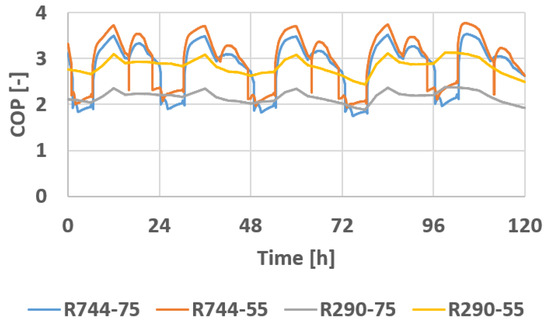
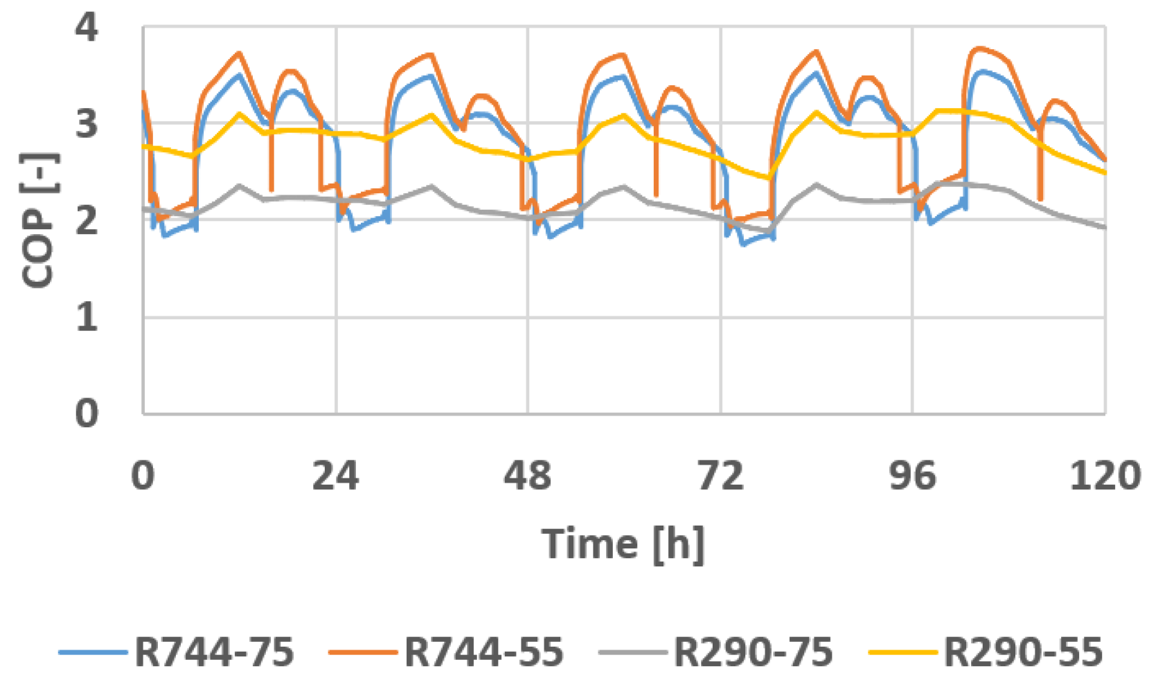
Figure 6 illustrates the variation in the COP of the heat pumps during the Int4 case.

Figure 6. The variation in the COP of the heat pumps during the Int4 case.

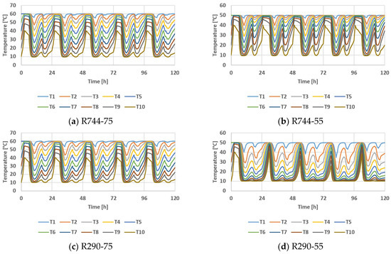
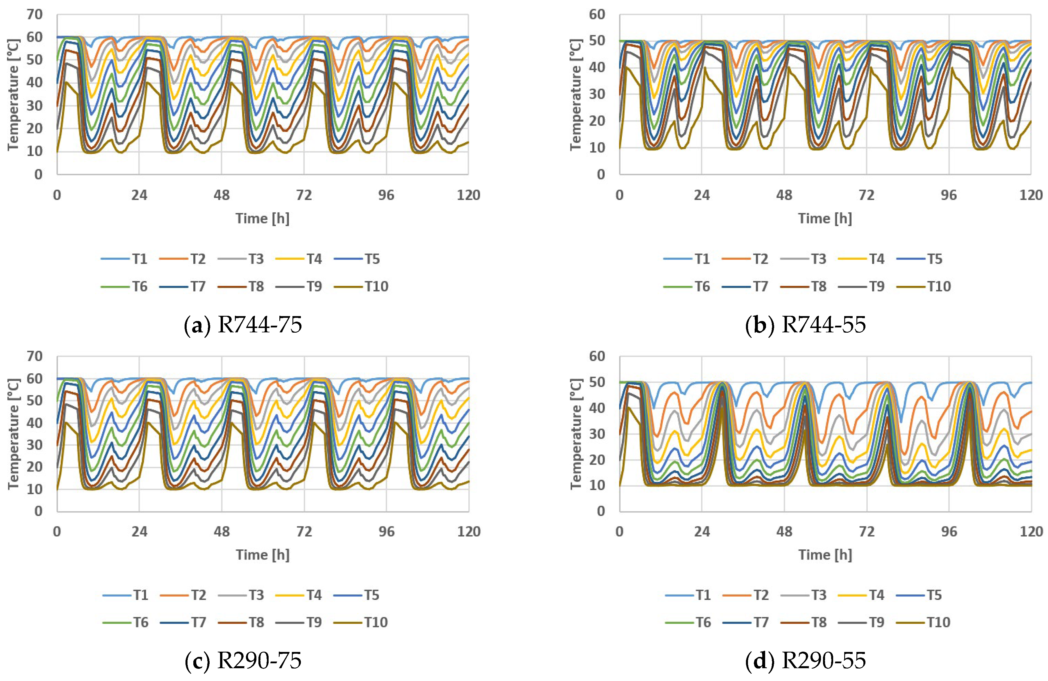
The hourly variations in temperature distribution in the layers of the storage tank for the Int4 case are presented in Figure 7.

Figure 7. The hourly variation in temperature distribution in the layers of the storage tank for Int4.

The produced thermal power and electrical power consumed by the heat pumps depend on the operating conditions, including the outdoor air temperature for each case, as well as the return water temperature for R744 and the supply water temperature for R290.

The heat-pump configurations were sized as the minimum number of units capable of covering the DHW consumption over the full range of operating conditions, with the storage tank buffering short-term peaks (Figure 6 and Figure 7). Extreme or atypical consumption days, as well as failure scenarios (e.g., temporary unavailability of one heat pump unit), were not explicitly evaluated and are noted here as a limitation for system design margins. In such situations the existing boiler, retained as a backup, would cover the missing demand.

Due to different operating conditions, the number of required heat pumps, as well as their characteristics and performance, differ as shown in Table 13.

Table 13. Number and characteristics of heat pumps.

Code Range		Int1	Int2	Int3	Int4	Int5	Int6
Daily average temperature [°C]		26.4–28.1	17.9–20.2	10.3–12.7	0.9–2.1	−7.2–−11.3	−7.6–−11.3
Characteristic daily average temperature [°C]		27.25	19.05	11.5	1.5	−9.25	−9.45
R744-75	Number of heat pumps [-]	2	2	2	2	2	2
	COP [-]	2.30–4.07	2.25–4.11	2.01–4.21	1.75–3.53	1.36–2.96	1.29–2.83
	Maximum thermal power [kW]	223	225	231	212	184	177
R744-55	Number of heat pumps [-]	2	2	2	2	2	2
	COP [-]	2.52–4.59	2.46–4.62	2.21–4.70	1.93–3.77	1.40–3.13	1.41–2.99
	Maximum thermal power [kW]	252	254	258	226	195	187
R290-75	Number of heat pumps [-]	3	3	3	4	5	5
	COP [-]	3.37–5.53	2.91–4.19	2.38–3.27	1.88–2.37	1.40–1.98	1.40–1.90
	Maximum thermal power [kW]	211	188	167	188	210	204
R290-55	Number of heat pumps [-]	2	2	3	3	4	4
	COP [-]	4.48–7.35	3.86–5.58	3.14–4.35	2.43–3.13	1.70–2.57	1.70–2.46
	Maximum thermal power [kW]	215	169	204	154	174	168

For the R744 configurations, two heat pumps operate for all 365 days in the R744-75 case, whereas the R744-55 case requires two heat pumps for 305 days and one heat pump for 60 days. For the R290 configurations, the R290-75 case needs three heat pumps for 243 days, four for 58 days, and five for 64 days, while the R290-55 case requires two heat pumps for 129 days, three for 172 days, and four for 58 days.

Despite the current DHW preparation system being equipped with a boiler with a thermal power of 1120 kW, by employing the storage system, it can also operate with heat pumps that produce maximum thermal powers in the range of (154–258) kW. The nominal capacity of 120 kW per R744 unit corresponds to the rating conditions, while the delivered thermal power depends on the outdoor and return temperatures. For this reason the maximum thermal power of the two units in Table 13 ranges from 177 to 258 kW, i.e., from about 89 to 129 kW per unit. The maximum of 258 kW occurs for R744-55 at the characteristic temperature of 11.5 °C (Int3), where each unit delivers more than its nominal power, whereas in the coldest intervals (Int5 and Int6), where the maximum is reached at the milder hours of the interval, each unit delivers less than 100 kW. All values lie within the range covered by the manufacturer data, so no extrapolation is involved.

4.3. Efficiency Analysis of the System

4.3.1. Heat Pump Operation Analysis for Cluj-Napoca

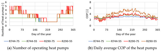
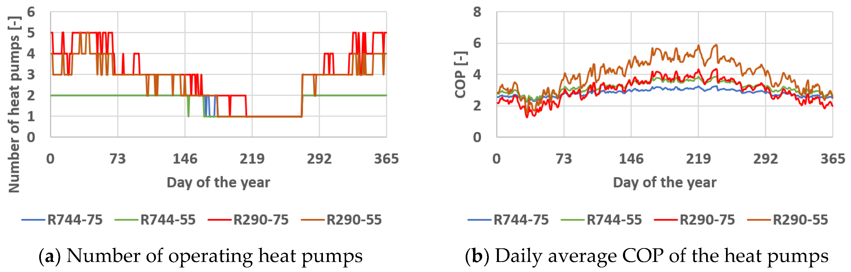
The results of simulating the annual behavior of the alternative DHW preparation system across the four configurations studied are presented as follows. The time step of the simulation was of 1 day. Figure 8 depicts the daily variation in the number of operating heat pumps and the daily average COP of the heat pumps.

Figure 8. The variation in the number of operating heat pumps and the daily average COP of the heat pumps.

The maximum number of required heat pumps reaches two for the R744 configurations and five for the R290 configurations, with the daily average COP varying in the range of 2.26–3.88 for R744 and 1.28–5.88 for R290, depending mostly on the ambient temperature.

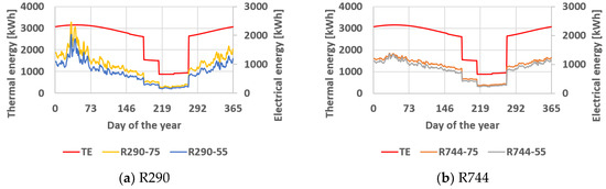
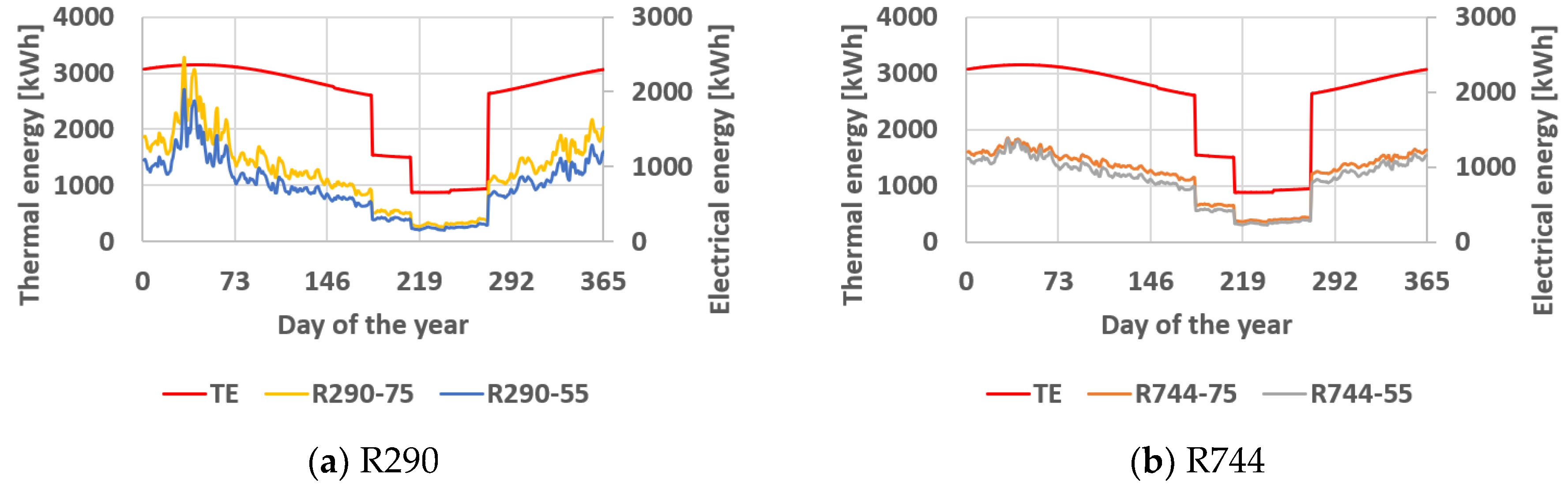
Figure 9 illustrates the variation in the daily average thermal energy produced by the heat pumps and the variation in the daily average electrical energy consumed by the heat pumps.

Figure 9. The variation in the daily average thermal energy produced by the heat pumps (TE) and average electrical energy consumed by the heat pumps.

The thermal energy produced by the heat pumps is similar to DHW consumption, with small annual variations caused by the variation in the cold-water temperature from the supply network. The electrical energy consumption is correlated with the COP of the heat pumps.

4.3.2. Photovoltaic System Operation Analysis

Table 14 summarizes the main technical characteristics of the photovoltaic system, including the maximum PV panel efficiency and the peak instantaneous electrical power.

Table 14. PV efficiency and peak power.

Country	Maximum PV Panel Efficiency [%]	Peak Instantaneous Electrical Power [kW]
ROU	23.8	102.9
PRT	22.6	100.8
SWE	23.5	97.8
USA	24.2	106.8
CHN	24.1	104.5
JPN	23.3	103.4
FRA	23.5	98.3
HUN	23.6	97.2

Table 15 presents the monthly values for the electric energy produced by the PV system.

Table 15. Monthly values for electricity production [MWh].

Month of the Year	1	2	3	4	5	6	7	8	9	10	11	12
ROU	1.5	4.1	8.6	9.4	13.9	11.6	14.3	15.8	11.1	8.2	4.1	1.6
PRT	7.1	9.1	13.1	9.2	13.7	15.5	17.6	18.5	15.7	11.6	9.7	4.4
SWE	0.0	1.8	5.7	11.6	13.2	12.6	10.1	8.1	7.9	3.2	0.1	0.0
USA	9.1	8.0	13.0	12.5	12.5	14.7	13.1	14.4	11.2	9.5	7.5	7.3
CHN	9.5	11.8	17.0	13.5	14.6	12.7	11.3	13.0	13.2	10.5	10.0	9.0
JPN	11.1	10.4	11.8	12.8	10.7	9.4	12.4	15.0	9.3	8.7	6.7	9.2
FRA	3.2	3.8	8.3	12.8	9.6	16.3	12.5	13.1	8.2	8.2	2.6	1.7
HUN	5.0	4.0	6.7	11.5	14.3	14.2	16.5	14.0	12.3	8.0	2.9	3.3

These values depend on the climatic data (available solar radiation and ambient temperatures) and on the technical characteristics of the PV panels and of the inverter.

4.3.3. Overall Results

Table 16 summarizes the annual values of electrical energy consumed by heat pumps (ELC) and electrical energy produced by photovoltaics (ELP).

Table 16. Heat-pump consumption and photovoltaic production.

Country	ELC				ELP
	R744-75	R744-55	R290-75	R290-55
[-]	[MWh]	[MWh]	[MWh]	[MWh]	[MWh]
ROU	329.4	295.6	339.5	260.0	104.2
PRT	264.2	229.7	230.4	173.2	145.2
SWE	345.4	310.6	354.6	270.9	74.5
USA	292.6	259.0	281.2	213.6	132.8
CHN	315.6	282.7	324.3	248.4	146.1
JPN	273.8	240.0	249.0	188.0	127.3
FRA	307.0	271.8	291.6	221.0	100.4
HUN	308.0	273.9	301.9	229.8	112.8

The annual electrical energy consumed by the heat pumps varies across the analyzed configurations and locations, ranging from 173.2 MWh to 354.6 MWh, while the annual electricity production from the photovoltaic system ranges between 74.5 MWh and 146.1 MWh.

The ambient temperature influences the heat pump COP and, consequently, the energy consumption, and energy prices (natural gas or electricity) fluctuate depending on the geographical location. The annual values of the heat pump COP in the targeted countries are presented in Table 17.

Table 17. The annual values of the heat pump COP in the targeted countries.

Country	R744-75	R744-55	R290-75	R290-55
ROU	2.74	3.05	2.66	3.47
PRT	2.92	3.36	3.35	4.46
SWE	2.71	3.02	2.64	3.46
USA	2.82	3.19	2.94	3.87
CHN	2.76	3.08	2.68	3.50
JPN	2.88	3.28	3.16	4.19
FRA	2.81	3.17	2.96	3.90
HUN	2.79	3.14	2.85	3.74

The annual average COP at which the heat pumps will operate varies depending on the country and configuration, ranging from 2.64 (for R290-75 in Sweden) to 4.46 (for R290-55 in Portugal), thereby justifying the high level of efficiency compared to a natural gas boiler.

The solar fraction is defined as the ratio of annual PV electricity generation to annual heat-pump electricity demand; it implicitly assumes that all PV electricity is used on site, either by the heat pumps or by other electrical loads of the campus, and does not account for inverter losses. Table 18 presents the SF provided by the photovoltaic system for the analyzed heat-pump configurations across the selected countries.

Table 18. SF for the analyzed heat-pump configurations across the selected countries.

Country	R744-75	R744-55	R290-75	R290-55
ROU	31.64%	35.25%	30.70%	40.08%
PRT	54.94%	63.20%	63.01%	83.82%
SWE	21.57%	23.99%	21.02%	27.51%
USA	45.40%	51.28%	47.25%	62.18%
CHN	46.30%	51.67%	45.04%	58.80%
JPN	46.51%	53.07%	51.15%	67.74%
FRA	32.71%	36.95%	34.44%	45.44%
HUN	36.62%	41.18%	37.36%	49.08%

When using photovoltaic solar collectors, their annual electricity production covers between 21.02% (for R290-75 in Sweden) and 83.82% (for R290-55 in Portugal) of the annual electricity needs of the heat pumps across the analyzed countries and configurations.

The solar fraction is an annual energy ratio and does not show whether PV electricity is available when the heat pumps operate. To check this, the operation of the heat pumps was simulated with a 1 min time step for two of the 5-day intervals defined in Section 3.2, a summer one (Int1, 23–27 August) and a winter one (Int6, 8–12 February), using the hourly PV power of the Typical Meteorological Year linearly interpolated to 1 min values. In the summer interval the PV system generates 2621 kWh, of which 47% to 82% is used directly by the heat pumps. The PV electricity covers directly 40% to 50% of their consumption, whereas the ratio of PV generation to heat-pump consumption would suggest 53% to 100%. The remaining 18% to 53% of the PV generation (478 to 1397 kWh) exceeds the heat pump demand at the moment of production, with instantaneous values up to 55 kW. In the winter interval the PV system generates 896 kWh, which covers 9% to 13% of the heat-pump consumption, and 93% to 99.8% of it is used directly, so the surplus does not exceed 7.3%. The surplus is not exported to the grid but used for other electrical loads of the campus, so no export and no curtailment occur, and all PV electricity enters the payback calculation as avoided purchase of grid electricity at the electricity price. This assumes that the other loads can absorb the surplus at any moment. The annual share of the surplus could not be determined from these two intervals.

The reduction in CO₂ emissions resulting from the use of heat pumps compared to the baseline level—both standalone and in combination with the photovoltaic system—is presented in Table 19, with cases where emission reductions do not apply being designated as not applicable (N.A.). The conversion factors from final energy to primary energy and standard electricity emission factors are necessary to evaluate the reduced amount of CO₂ [52].

Table 19. The reduction in CO₂ emissions resulting from the use of heat pumps compared to the baseline level.

Country	fconv		fem		Use of Heat Pumps				Use of Heat Pumps and PV System
	Value	Ref.	Value	Ref.	R744-75	R744-55	R290-75	R290-55	R744-75	R744-55	R290-75	R290-55
ROU	2.5	[53]	0.212	[54,55]	34.48%	41.20%	32.48%	48.28%	55.21%	61.93%	53.21%	69.01%
PRT	2.5	[56]	0.067	[55]	79.37%	82.07%	82.02%	86.48%	90.71%	93.40%	93.35%	97.81%
SWE	1.8	[57]	0.008	[55]	98.00%	98.20%	97.95%	98.43%	98.43%	98.63%	98.38%	98.86%
USA	2.8	[58]	0.384	[59]	N.A.	N.A.	N.A.	N.A.	17.47%	34.81%	23.39%	58.27%
CHN	2.93	[60]	0.525	[59]	N.A.	N.A.	N.A.	N.A.	N.A.	13.03%	N.A.	34.86%
JPN	2.71	[61]	0.477	[59]	N.A.	N.A.	N.A.	N.A.	13.49%	33.47%	28.15%	64.18%
FRA	1.9	[62]	0.031	[55]	92.45%	93.32%	92.83%	94.57%	94.92%	95.79%	95.30%	97.04%
HUN	2.5	[63]	0.131	[55]	53.50%	58.65%	54.42%	65.30%	70.53%	75.67%	71.45%	82.33%

Notations: f_conv—electricity conversion factor from final energy to primary energy [-]; f_em—standard electricity emission factor [t_CO2/MWh]; N.A.—not applicable.

The primary-energy conversion factor (f_conv) and standard electricity emission factor (f_em) used for each country are reported in Table 19. The CO₂ balance considers only operational emissions; embodied emissions from the manufacturing of the PV panels and heat pumps are not included and are noted here as a limitation.

When using heat pumps powered by electricity from the grid, CO₂ emissions are reduced by between 32.48% (for R290-75 in Romania) and 98.43% (for R290-55 in Sweden), and in the case of coupling the heat pumps to a photovoltaic system, a CO₂ reduction ranging from 13.03% (for R744-55 in China) to 98.86% (for R290-55 in Sweden) is achieved across the analyzed countries and configurations.

The N.A. entries in the “Use of Heat Pumps” columns for the USA, China, and Japan indicate that, without PV, the standalone heat pump does not reduce CO₂ emissions relative to the gas boiler baseline: the national electricity emission factor (f_em) in these grids is high enough that electricity-based emissions exceed the avoided gas emissions. A net reduction is achieved only once PV self-generation is added, lowering effective grid dependence, as shown in the corresponding “Use of Heat Pumps and PV” columns, except for China with R744-75 and R290-75, where the reduction remains not applicable even with PV.

4.4. Economic Analysis

Table 20 presents the payback period in years for replacing boilers with heat pumps, while Table 21 shows the payback period in years for replacing boilers with heat pumps combined with the photovoltaic system. Cases where the investment cannot be recovered at all are designated as N.A. (not applicable).

Table 20. The payback period [years] for replacing boilers with heat pumps.

Country	R	D	R744-75	R744-55	R290-75	R290-55
ROU	0.29	135.90	N.A.	25.9	N.A.	5.8
PRT	0.53	112.50	2.8	2.4	1.4	0.9
SWE	0.80	52.60	1.0	1.0	0.6	0.4
USA	0.23	146.00	N.A.	N.A.	N.A.	15.7
CHN	0.51	44.00	4.5	4.0	2.7	1.6
JPN	0.27	182.00	N.A.	23.5	20.1	3.8
FRA	0.49	136.60	2.8	2.4	1.5	0.9
HUN	0.30	73.30	174.7	36.6	60.6	8.4

Notations: R—ratio between gas price/electricity price [-]; D—difference between electricity price and gas price [€/MWh]; N.A.—not applicable.

Table 21. The payback period [years] for replacing boilers with heat pumps and photovoltaic system.

Country	R	D	R744-75	R744-55	R290-75	R290-55
ROU	0.29	135.90	14.3	10.8	12.0	5.9
PRT	0.53	112.50	2.9	2.7	2.0	1.6
SWE	0.80	52.60	1.7	1.6	1.4	1.1
USA	0.23	146.00	22.0	15.5	15.2	8.1
CHN	0.51	44.00	5.2	4.8	4.1	3.2
JPN	0.27	182.00	11.3	8.9	7.5	4.9
FRA	0.49	136.60	3.6	3.3	2.7	2.0
HUN	0.30	73.30	22.4	17.5	16.2	9.4

Notations: R—ratio between gas price/electricity price [-]; D—difference between electricity price and gas price [€/MWh].

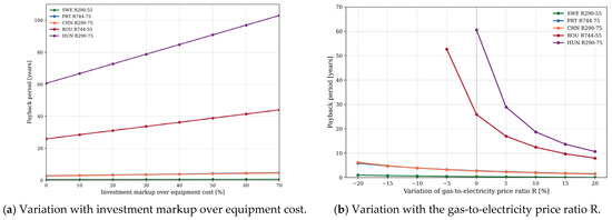
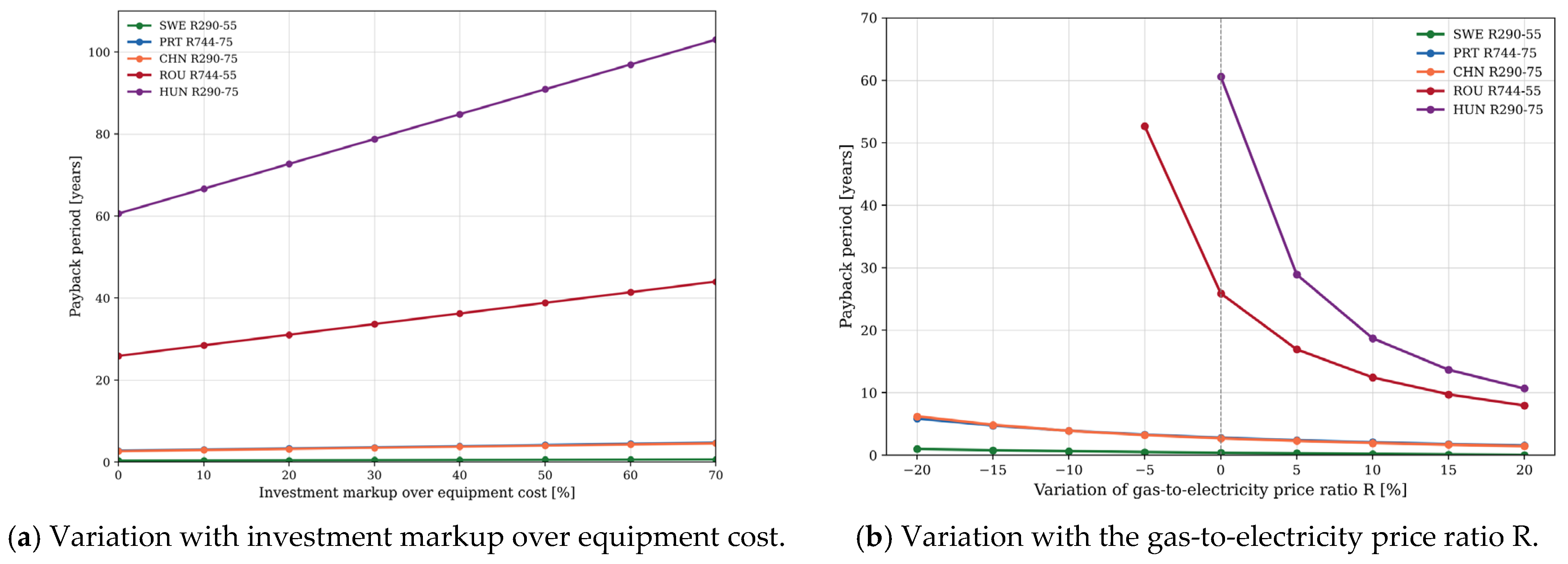
The investment I (Equation (22)) includes only equipment purchase cost. Figure 10 presents a sensitivity analysis using Equation (21) to estimate the effect of (a) an installation, upgrade and maintenance markup over equipment cost, from +10% to +70%, and (b) a ±20% variation in the gas-to-electricity price ratio. The markup range is based on reported cost breakdowns, in which the heat pump unit represents 38–54% of the total investment and the heat-source connection up to about 35% [64]. Excluding the heat-source connection, this corresponds to a markup of about 20–70% over the unit cost. Short-payback cases remain favorable under both variations, while cases already close to break-even (Table 20) are sensitive to realistic cost and price variation.

Figure 10. Sensitivity of the payback period, calculated using Equation (21), for five representative country/configuration cases covering short, intermediate and long payback periods in Table 20.

Overall, Figure 10 shows that the reported payback periods are robust to realistic cost and price uncertainty for the configurations already identified as economically favorable, while the small subset of cases close to the break-even threshold (Table 20) should be interpreted with corresponding caution. A 50% investment markup increases every payback period by 50%, and a markup of 70%, the upper limit of the literature range, by 70%, while a decrease in R by 5% makes the payback of Hungary R290-75 undefined. Replacement costs and financing are not included, and local incentives are not considered. Incentives would shorten the payback, while financing costs would lengthen it.

The heat demand Q entering Equation (22) is the occupancy-adjusted demand of Section 4.1, in which the calculated July–September values were replaced by the measured ones. For a campus fully occupied throughout the year, the demand would be about 15% higher (1296 instead of 1128 MWh gas-equivalent). Since Π ∝ 1/Q, the payback periods in Table 20 would then be about 13% shorter, and those in Table 21 would also be affected.

Table 20 reports the calculated payback period without reference to equipment service life. Assuming a reference technical lifetime of 20 years for the heat pump units, six further configurations, beyond the six already reported as N.A. (R < R_be), show a finite payback period exceeding this lifetime (Romania R744-55: 25.9 years, Japan R744-55: 23.5 years, Japan R290-75: 20.1 years, Hungary R744-75/R744-55/R290-75: 174.7/36.6/60.6 years). These twelve cases in total (38% of the 32 analyzed) would not recover the investment within the expected equipment lifetime and should be regarded as economically non-viable, independent of the price and cost-sensitivity discussed in Figure 10.

In the scenario of replacing the boiler with heat pumps, the payback period ranges from 0.4 to 174.7 years across the analyzed countries and valid configurations, whereas coupling the heat pumps with a photovoltaic system results in a payback period ranging from 1.1 to 22.4 years.

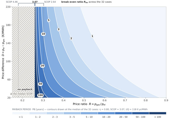
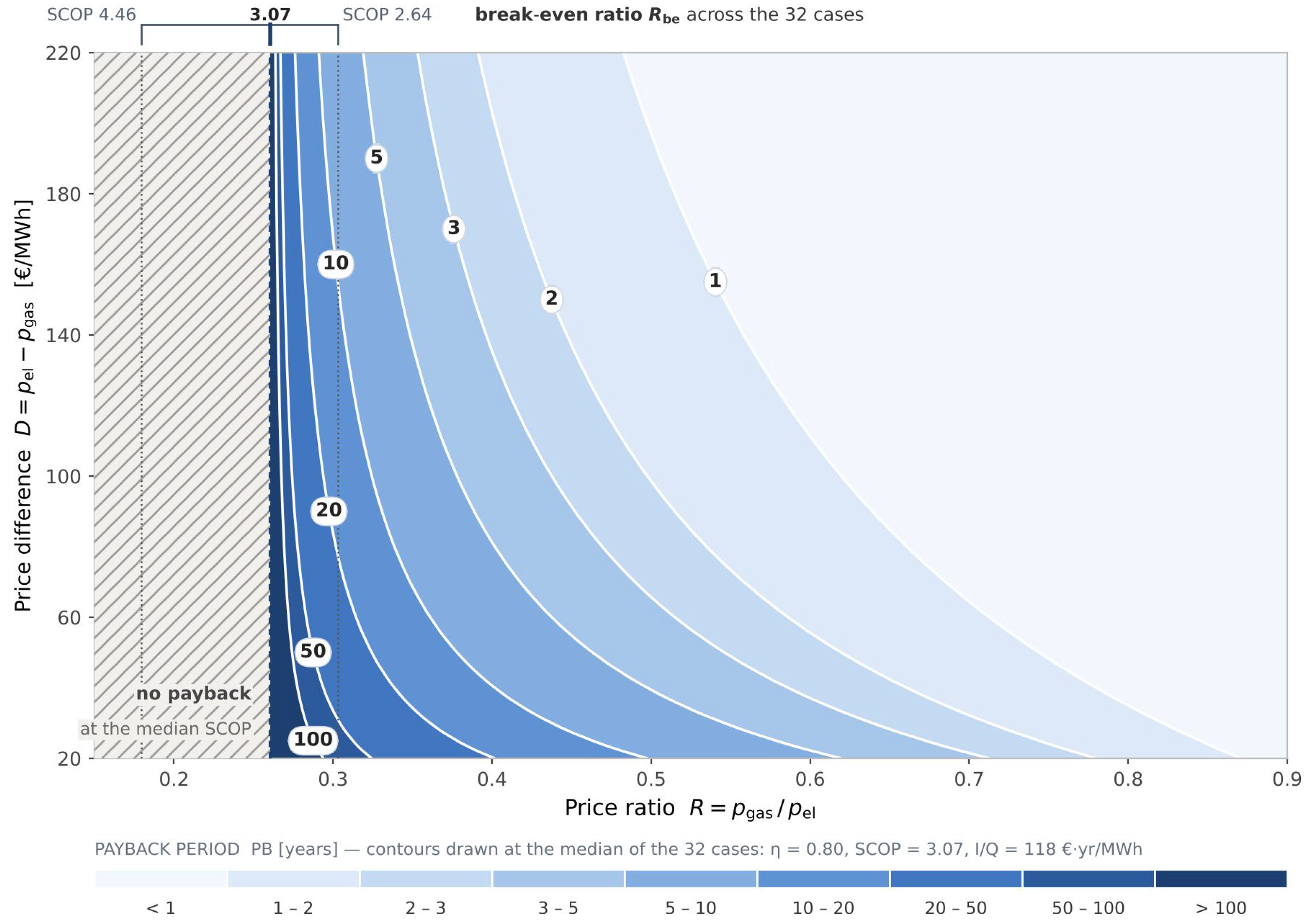
Figure 11 illustrates the payback curves as a function of R and D. The map shows why the two price variables do not have symmetric status even though they occupy the axes symmetrically. The difference D enters linearly: at constant R the payback period is simply inversely proportional to it and doubling the price difference halves the payback. The ratio R, by contrast, enters through the denominator (R − R_be), which is why the iso-payback curves crowd together near the asymptote. All the non-linearity of the problem therefore resides in the price ratio; the price difference merely scales the result.

Figure 11. The payback period for heat-pump replacement as a function of R and D, plotted at the medians of the 32 cases (η = 0.80, SCOP = 3.07, I/Q = 118 € · year/MWh).

Since PB is inversely proportional to D but varies as 1/(R − R_be), all the non-linearity of the problem resides in the price ratio. The bracket above the plot gives the range within which the break-even ratio falls over the set analyzed, from SCOP = 4.46 to SCOP = 2.64; the heavy dashed line marks the median value. Hatched area: below the median break-even ratio, where the replacement does not pay back.

The wide range of payback periods across countries (Table 20) follows directly from the non-linear R–R_be relationship discussed in Figure 11: cases with R well above R_be (e.g., Portugal) yield short paybacks, while cases with R close to R_be (e.g., Hungary) yield disproportionately long ones. This sensitivity is quantified in Figure 10b. The break-even outdoor temperatures in Section 4.2 show the same effect within a single location. For Cluj-Napoca, the boiler is the cheaper heat source below 10.1 °C for R290-75 and below 0.7 °C for R290-55, but only below −0.4 °C for R744-75 and below −3.4 °C for R744-55. The payback periods in Table 20 are calculated with the annual COP, that is, for heat pumps operating throughout the year, and do not account for the possible use of the cheaper boiler in these periods.

The COP fitting uncertainty reported in Section 3.2 (up to 0.30% for R744 and 9.48% for R290) does not affect the payback period uniformly but propagates through the break-even ratio R_be = η/SCOP. Recalculating Equation (21) for all 32 cases under this uncertainty shows that configurations with short payback periods (below approximately 5 years) are robust, changing by less than 20%, with the exception of Japan R290-55 (from 3.8 to 5.0 years). The configurations closest to the break-even threshold are sensitive enough for the price ratio R to cross R_be, rendering their payback undefined rather than a fixed number of years (Japan R290-75 and Hungary R290-75), or, in the opposite direction, defined (Romania R290-75). These specific cases should therefore be read as indicating economic marginality rather than a precise payback estimate.

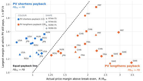
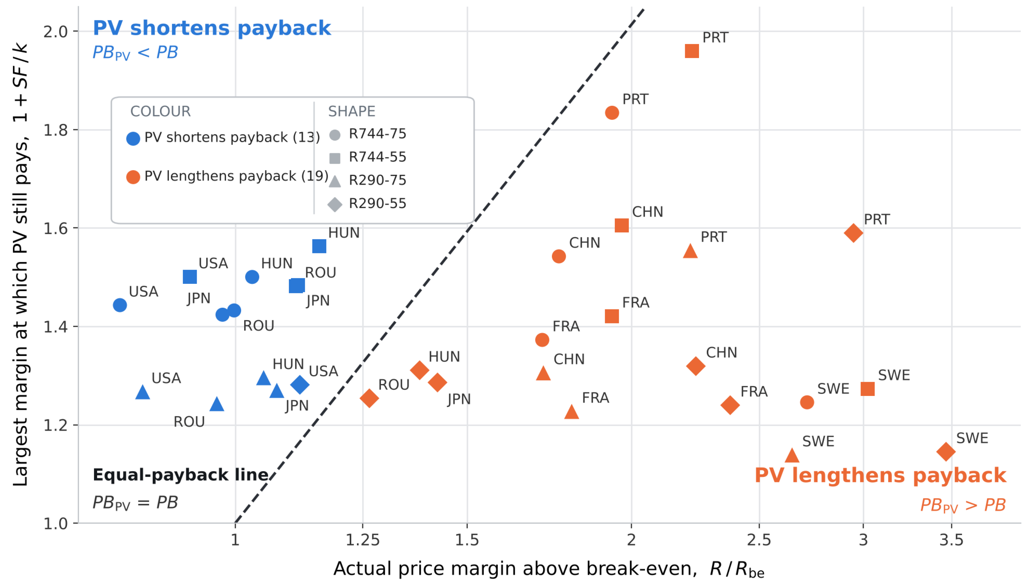
Figure 12 presents the criterion R/R_be < 1 + SF/k graphically. k represents the ratio of the investment in the photovoltaic system to the investment in the heat pumps. The two axes represent the same quantity—the margin above the break-even threshold—in its actual value and in the largest value at which photovoltaics remain justified; the diagonal is the locus on which the two payback periods are equal.

Figure 12. Effect of the photovoltaic system on the payback period for the 32 cases analyzed.

A system pays back faster with photovoltaics only if its actual margin above the break-even ratio, R/R_be, is smaller than 1 + SF/k, that is, only for points lying above the equal-payback line. The criterion is independent of both the annual heat demand Q and the price difference D and classifies all 32 cases without exception. Color indicates the photovoltaic decision; marker shape the heat pump variant. A systematic vertical ordering of the marker shapes within each country can be observed: the R744 variants lie above the R290 ones, and within each refrigerant the variant with higher SCOP lies higher, because the solar fraction increases with heat pump performance. The usefulness threshold of the photovoltaic system is therefore the more permissive the better the heat pump performs. The photovoltaic system shortens the payback period if and only if R/R_be < 1 + SF/k. The criterion depends on neither the heat demand nor the price difference and classifies all 32 cases without exception: 13 favorable and 19 unfavorable to photovoltaics. All 13 favorable cases are located in the four countries with the lowest price ratio (Romania, USA, Japan and Hungary), where the margin R/R_be is below 1.2, whereas all unfavorable cases show a margin above 1.2.

According to the data presented in Table 22, the cost reduction for DHW preparation varies significantly depending on the country and the chosen heat-pump configuration.

Table 22. Percentage reduction in DHW preparation cost.

Country	Use of Electricity from the Grid				Use of Electricity from the Grid and PV
	R744-75	R744-55	R290-75	R290-55	R744-75	R744-55	R290-75	R290-55
ROU	N.A.	10.04%	N.A.	20.87%	31.47%	41.75%	28.41%	52.59%
PRT	48.31%	55.06%	54.93%	66.12%	76.71%	83.46%	83.33%	94.52%
SWE	63.25%	66.95%	62.27%	71.17%	71.18%	74.88%	70.20%	79.10%
USA	N.A.	N.A.	N.A.	10.66%	33.18%	47.22%	37.97%	66.21%
CHN	43.24%	49.14%	41.66%	55.31%	69.52%	75.42%	67.93%	81.59%
JPN	N.A.	10.42%	7.06%	29.82%	45.33%	57.95%	54.59%	77.36%
FRA	41.55%	48.26%	44.49%	57.93%	60.67%	67.38%	63.61%	77.05%
HUN	2.85%	13.59%	4.76%	27.50%	38.43%	49.17%	40.34%	63.08%

Notations: N.A.—not applicable.

With the heat pumps covering the whole DHW demand in the simulated scenario, and the boiler kept only as a backup, the cost of DHW preparation is reduced by 2.85% to 71.17% across the analyzed countries and configurations due to the low electrical energy consumption. Coupling the heat pumps with a photovoltaic system, located on the roof of one of the dormitories or the cafeteria, allows for a cost reduction ranging from 28.41% to 94.52%.

5. Conclusions

To the best of the authors’ knowledge, this is the first study investigating the thermal behavior of high-temperature air-to-water heat pumps using CO₂ and propane as refrigerants in buildings characterized by high DHW consumption across different supply temperature regimes.

The study develops empirical equations to calculate the thermal power generated by the investigated air-to-water heat pumps and their COPs, derived directly from manufacturers’ technical data. For the CO₂ systems operating on a transcritical cycle, these equations are functions of both the ambient temperature and the return temperature, with the latter being particularly significant. The coefficients were fitted separately for return temperatures up to 25 °C, where the quadratic term vanishes, and above 25 °C. In contrast, for the propane systems, the equations are formulated as functions of the ambient temperature and the supply temperature. Compared with the manufacturers’ data, the maximum deviations are 0.30% for the COP and 2.33% for the thermal power of the CO₂ units, and 9.48% for the COP and 2.31% for the thermal power of the propane units, while the mean absolute percentage deviations over the 212 data points are 0.92% for the COP and 0.24% for the thermal power. The equations are valid only for the dataset used for their derivation.

The investigation method is original because it proposes a new calculation method for the daily variation in thermal energy production and the daily average COP. These are expressed as functions of the daily average temperature, derived from simulations of heat pumps thermal behavior with a one-minute time step over consecutive days with nearly identical ambient temperature variations. The simulations cover the full range of operating conditions of the heat pumps, so the resulting daily equations do not depend on the location.

The study presents the simulation of the current DHW preparation system in the Marasti student complex of TUCN, as well as the upgraded system using high-temperature heat pumps—employing either CO₂ or propane as refrigerants—coupled with a storage tank and a photovoltaic system. The share of energy consumption for DHW preparation is approximately 50 ± 10% of the total thermal energy consumption of the campus, varying with heating needs that are contingent on external temperature values.

The upgraded system uses either R744 (operating on a transcritical cycle with two units of 120 kW each) or R290 (with five units of 60 kW for the 75 °C scenario or four units of 60 kW for the 55 °C scenario). With the storage tank, the heat pumps, whose maximum thermal power ranges between 154 and 258 kW, cover the DHW demand of the analyzed operating conditions, while the existing gas boiler is retained as a backup for peak loads, extreme consumption days and failure situations. The annual COP ranges between 2.71 and 2.92 for R744-75, between 3.02 and 3.36 for R744-55, between 2.64 and 3.35 for R290-75, and between 3.46 and 4.46 for R290-55. Integrating a photovoltaic system covers a share of the annual electricity demand (solar fraction) ranging across the targeted countries between 21.57% and 54.94% for R744-75, 23.99% and 63.20% for R744-55, 21.02% and 63.01% for R290-75, and 27.51% and 83.82% for R290-55.

In the simulated scenario, the heat pumps supply the DHW demand and the gas boiler is retained only as a backup. The cost of DHW preparation is reduced by 2.85% to 71.17% with heat pumps alone and by 28.41% to 94.52% with photovoltaic integration. The CO₂ emissions are reduced by 32.48% to 98.43% with heat pumps alone, in the locations where a reduction is achieved, and by 13.03% to 98.86% with photovoltaic integration. In the USA, China and Japan, where the electricity grid is carbon-intensive, a reduction is achieved only with photovoltaic coupling, and not even then in China for R744-75 and R290-75.

The economic evaluation is based on a simple undiscounted payback period that accounts for the equipment cost only. The payback periods range from 0.4 to 174.7 years for heat pumps alone and from 1.1 to 22.4 years with photovoltaic integration. For heat pumps alone, the payback period is not applicable in 6 of the 32 cases and exceeds 20 years in 6 further cases, so 12 of the 32 cases (38%) are not economically attractive. Photovoltaic integration shortens the payback period in 13 of the 32 cases. The sensitivity analysis considered equipment markups of up to 70% and variations of ±20% in the energy price ratio, as well as the propagation of the COP uncertainty. For the cases with a payback period below 5 years, the COP uncertainty changes the payback period by less than 20%, except for Japan with R290-55. The parametric analysis reveals that the payback period is inversely proportional to the energy price difference, while its non-linear behavior is driven by the energy price ratio through the break-even threshold term. Integrating a photovoltaic system shortens the payback period if and only if the price ratio relative to the break-even value remains below the threshold defined by the solar fraction and the investment cost ratio. This criterion is independent of both the annual heat demand and the price differences.

The reported CO₂ reductions rely on national annual average emission factors (Table 19) and do not reflect regional grid variation or hourly carbon intensity. Future grid decarbonization would increase the reductions where they are already positive, but it could change the outcome in the cases where the standalone heat pump currently shows no reduction (USA, China and Japan). Refrigerant leakage over the equipment lifetime was not included in the balance. Since both refrigerants have a very low GWP, direct emissions are expected to be small compared with indirect ones, but this was not quantified. The units considered are monobloc and installed outdoors. Even so, a multi-unit R290 installation (up to 5 units) requires dedicated safety provisions, such as charge limits, installation clearances, hazardous-zone provisions and leak detection, which fall outside the scope of this analysis. The storage tank volume of 28 m³ was not validated against measured data, and the thermal losses of the tank and of the distribution network were neglected. The site-specific elements of this study are the magnitude and profile of the heat demand, including seasonal occupancy, the existing boiler and storage tank, the PV array size and the investment cost. Climate, energy prices and emission factors were varied across eight locations, and the payback and PV criteria are independent of installation size. The absolute results (CO₂ saved, payback and solar fraction) are therefore specific to this campus, and their transfer to other consumers requires re-evaluating these inputs.

DHW preparation using high-temperature heat pumps, a storage tank and a photovoltaic system represents a promising energy-efficient solution for the investigated student campus, with the existing gas boiler retained as a backup for extreme situations. Extreme consumption days, failure scenarios and embodied emissions were not evaluated in this study. The results therefore demonstrate strong potential rather than a fully validated replacement for the existing gas-based system, and their transfer to other consumers should be assessed case by case.

References

- Zarco-Periñán, P.J.; Zarco-Soto, F.J.; Zarco-Soto, I.M.; Martínez-Ramos, J.L.; Sánchez-Durán, R. CO2 Emissions in Buildings: A Synopsis of Current Studies. Energies 2022, 15, 6635. [Google Scholar] [CrossRef] [Scilit]
- IEA Greenhouse Gas Emissions from Energy Data Explorer. Available online: https://www.iea.org/data-and-statistics/data-tools/greenhouse-gas-emissions-from-energy-data-explorer (accessed on 25 September 2023).
- Karel, J.; Lucia, S. Institutional Description of the European Green Deal Investment Plan Framework; ZBW – Leibniz Information Centre for Economics: Kiel, Germany, 2022. [Google Scholar]
- Minetto, S. Theoretical and Experimental Analysis of a CO2 Heat Pump for Domestic Hot Water. Int. J. Refrig. 2011, 34, 742–751. [Google Scholar] [CrossRef] [Scilit]
- Cui, Q.; Wei, D.; Gao, E.; Zhang, X. Compressor Control Strategy for CO2 Heat Pump toward Efficient and Stable Domestic Hot Water Production: An Experimental Investigation. Therm. Sci. Eng. Prog. 2023, 38, 101681. [Google Scholar] [CrossRef] [Scilit]
- Yang, D.; Song, Y.; Cao, F.; Jin, L.; Wang, X. Theoretical and Experimental Investigation of a Combined R134a and Transcritical CO2 Heat Pump for Space Heating. Int. J. Refrig. 2016, 72, 156–170. [Google Scholar] [CrossRef] [Scilit]
- Velasco, F.J.S.; Haddouche, M.R.; Illán-Gómez, F.; García-Cascales, J.R. Experimental Characterization of the Coupling and Heating Performance of a CO2 Water-to-Water Heat Pump and a Water Storage Tank for Domestic Hot Water Production System. Energy Build. 2022, 265, 112085. [Google Scholar] [CrossRef] [Scilit]
- Olympios, A.V.; Hoseinpoori, P.; Markides, C.N. Toward Optimal Designs of Domestic Air-to-Water Heat Pumps for a Net-Zero Carbon Energy System in the UK. Cell Rep. Sustain. 2024, 1, 100021. [Google Scholar] [CrossRef] [Scilit]
- Bani Issa, A.A.; Liang, C.; Groll, E.A.; Ziviani, D. Residential Heat Pump and Air Conditioning Systems with Propane (R290) Refrigerant: Technology Review and Future Perspectives. Appl. Therm. Eng. 2025, 266, 125560. [Google Scholar] [CrossRef] [Scilit]
- Leonzio, G.; Fennell, P.S.; Shah, N. Air-Source Heat Pumps for Water Heating at a High Temperature: State of the Art. Sustain. Energy Technol. Assess. 2022, 54, 102866. [Google Scholar] [CrossRef] [Scilit]
- Ferrara, M.; Babuin, M.; Fabrizio, E.; Corgnati, S.P. Assessing the Decarbonization Potential of New Generation R290 High-Temperature Heat Pumps for Apartment Buildings. Energy Rep. 2025, 13, 2095–2105. [Google Scholar] [CrossRef] [Scilit]
- Conte, R.; Zanetti, E.; Tancon, M.; Azzolin, M. Comparative Analysis of CO2 and Propane Heat Pumps for Water Heating: Seasonal Performance of Air and Hybrid Solar-Air Systems. Appl. Therm. Eng. 2025, 278, 127131. [Google Scholar] [CrossRef] [Scilit]
- Pop, O.G.; Balan, M.C. A Numerical Analysis on the Performance of DHW Storage Tanks with Immersed PCM Cylinders. Appl. Therm. Eng. 2021, 197, 117386. [Google Scholar] [CrossRef] [Scilit]
- Zou, L.; Liu, Y.; Yu, J. Recent Advances on Performance Enhancement of Propane Heat Pump for Heating Applications. Energy 2025, 314, 134251. [Google Scholar] [CrossRef] [Scilit]
- Dehghan, A.A.; Barzegar, A. Thermal Performance Behavior of a Domestic Hot Water Solar Storage Tank during Consumption Operation. Energy Convers. Manag. 2011, 52, 468–476. [Google Scholar] [CrossRef] [Scilit]
- Liang, J.; Li, T. Detailed Transient Study of a Transcritical CO2 Heat Pump for Low-Carbon Building Heating. Buildings 2025, 15, 3489. [Google Scholar] [CrossRef] [Scilit]
- Atienza-Márquez, A.; Domínguez Muñoz, F.; Fernández Hernández, F.; Cejudo López, J.M. Domestic Hot Water Production System in a Hospital: Energy Audit and Evaluation of Measures to Boost the Solar Contribution. Energy 2022, 261, 125275. [Google Scholar] [CrossRef] [Scilit]
- Yang, Q.; Salenbien, R.; Motoasca, E.; Smith, K.; Tunzi, M. Development and Test: Future-Proof Substation Designs for the Low-Temperature Operation of Domestic Hot Water Systems with a Circulation Loop. Energy Build. 2023, 298, 113490. [Google Scholar] [CrossRef] [Scilit]
- Behzadi, A.; Arabkoohsar, A.; Yang, Y. Optimization and Dynamic Techno-Economic Analysis of a Novel PVT-Based Smart Building Energy System. Appl. Therm. Eng. 2020, 181, 115926. [Google Scholar] [CrossRef] [Scilit]
- Mi, P.; Zhang, J.; Gao, J.; Han, Y. Study on Optimal Allocation of Solar Photovoltaic Thermal Heat Pump Integrated Energy System for Domestic Hot Water. Renew. Energy 2023, 219, 119433. [Google Scholar] [CrossRef] [Scilit]
- Ma, S.; Lu, S.; Ma, D.; Li, C.; Liu, C.; Wu, L.; Chen, M.; Xu, C.; Ma, H. Investigation on the Thermal Performance and Economy of a Solar Assisted Air Source Heat Pump Domestic Hot Water System. Appl. Therm. Eng. 2023, 232, 121007. [Google Scholar] [CrossRef] [Scilit]
- Guo, X.; Goumba, A.P. Air Source Heat Pump for Domestic Hot Water Supply: Performance Comparison between Individual and Building Scale Installations. Energy 2018, 164, 794–802. [Google Scholar] [CrossRef] [Scilit]
- Aguilar, F.J.; Aledo, S.; Quiles, P.V. Experimental Study of the Solar Photovoltaic Contribution for the Domestic Hot Water Production with Heat Pumps in Dwellings. Appl. Therm. Eng. 2016, 101, 379–389. [Google Scholar] [CrossRef] [Scilit]
- Chae, S.; Bae, S.; Nam, Y. Economic and Environmental Analysis of the Optimum Design for the Integrated System with Air Source Heat Pump and PVT. Case Stud. Therm. Eng. 2023, 48, 103142. [Google Scholar] [CrossRef] [Scilit]
- Belmonte, J.F.; Ramírez, F.J.; Almendros-Ibáñez, J.A. A Stochastic Thermo-Economic Analysis of Solar Domestic Hot-Water Systems in Compliance with Building Energy Code Requirements: The Case of Spain. Sustain. Energy Technol. Assess. 2022, 52, 102007. [Google Scholar] [CrossRef] [Scilit]
- Battaglia, V.; Vanoli, L.; Verde, C.; Nithiarasu, P.; Searle, J.R. Dynamic Modelling of Geothermal Heat Pump System Coupled with Positive-Energy Building. Energy 2023, 284, 128557. [Google Scholar] [CrossRef] [Scilit]
- Carbonell, D.; Haller, M.Y.; Philippen, D.; Frank, E. Simulations of Combined Solar Thermal and Heat Pump Systems for Domestic Hot Water and Space Heating. Energy Procedia 2014, 48, 524–534. [Google Scholar] [CrossRef] [Scilit]
- Kropp, M.; Lämmle, M.; Herkel, S.; Henning, H.M.; Velte-Schäfer, A. Enhancing Heat Pump Performance for Domestic Hot Water Preparation: A Comparative Analysis in Existing Multi-Family Houses. Energy Build. 2025, 328, 115155. [Google Scholar] [CrossRef] [Scilit]
- Rubina, A.; Pírek, O.; Salajka, R.; Rubinová, O.; Formánek, M.; Smutková, K. Case Study of Two Domestic Hot Water Storage Concepts in Residential Heat Pump Systems. Buildings 2026, 16, 1034. [Google Scholar] [CrossRef] [Scilit]
- Yang, S.K.; Kang, Y.H.; Ahn, Y.C. Achieving Energy Self-Sufficiency in a Dormitory Building: An Experimental Analysis of a PV–AWHP-ERV Integrated System. Buildings 2024, 14, 882. [Google Scholar] [CrossRef] [Scilit]
- Högnabba, K.; Tveit, T.M.; Vittor, S.; Zevenhoven, R. Economic and Environmental Considerations for the Deployment of Industrial Very High Temperature Heat Pumps in European Markets. Energy 2024, 309, 133147. [Google Scholar] [CrossRef] [Scilit]
- Letz, C.; Rode, J.; Römer, D. Heat Pumps Are Gaining Ground in Europe—Electricity Prices Matter; KfW Research Focus Economics No. 487; KfW Bankengruppe: Frankfurt am Main, Germany, 2025. [Google Scholar]
- Rosenow, J.; Barnes, J.; Galvin, R.; O’Mara, S.; Lowes, R. Total Cost of Ownership of Heat Pumps and Policy Choice: The Case of Great Britain. iScience 2025, 28, 111784. [Google Scholar] [CrossRef] [Scilit] [PubMed]
- Standard’s EN 378-1:2016; Refrigerating Systems and Heat Pumps—Safety and Environmental Requirements—Part 1: Basic Requirements, Definitions, Classification and Selection Criteria. European Committee for Standardization (CEN): Brussels, Belgium, 2016.
- Standard’s EN IEC 60335-2-40:2024; Household and similar electrical appliances – Safety – Part 2-40: Particular requirements for electrical heat pumps, air-conditioners and dehumidifiers. CENELEC: Brussels, Belgium, 2025.
- Department of Energy & Climate Change. Measurement of Domestic Hot Water Consumption in Dwellings; GOV.UK: London, UK, 2008. [Google Scholar]
- Hendron, R.; Anderson, R.; Christensen, C.; Eastment, M.; Reeves, P. Development of an Energy Savings Benchmark for All Residential End-Uses. In Proceedings of the SimBuild 2004, IBPSA-USA National Conference, Boulder, CO, USA, 4–6 August 2004. NREL/CP-550-35917. [Google Scholar]
- JRC Photovoltaic Geographical Information System (PVGIS)—European Commission. Available online: https://re.jrc.ec.europa.eu/pvg_tools/en/tools.html (accessed on 22 March 2024).
- Eicker, U. Solar Technologies for Buildings. Sol. Technol. Build. 2005, 8, 1–323. [Google Scholar] [CrossRef] [Scilit]
- Hiris, D.P.; Pop, O.G.; Balan, M.C. Analytical Modeling and Validation of the Thermal Behavior of Seasonal Storage Tanks for Solar District Heating. Energy Rep. 2022, 8, 741–755. [Google Scholar] [CrossRef] [Scilit]
- Hiris, P.D.; Bode, F.; Pop, O.G.; Balan, M.C. Simple Modeling of the Solar Seasonal Thermal Storage Behavior. In Proceedings of the Solar Energy Conversion in Communities; Visa, I., Duta, A., Eds.; Springer International Publishing: Cham, Switzerland, 2020; pp. 21–34. [Google Scholar]
- Sinha, R.; Bak-Jensen, B.; Pillai, J.R.; Zareipour, H. Flexibility from Electric Boiler and Thermal Storage for Multi Energy System Interaction. Energies 2019, 13, 98. [Google Scholar] [CrossRef] [Scilit]
- Kays, W.; Crawford, M.; Weigand, B. Convective Heat and Mass Transfer, 4th ed.; McGraw-Hill: Singapore, 2005. [Google Scholar]
- Hiris, D.P.; Pop, O.G.; Dobrovicescu, A.; Dudescu, M.C.; Balan, M.C. Modelling of Solar Assisted District Heating System with Seasonal Storage Tank by Two Mathematical Methods and with Two Climatic Data as Input. Energy 2023, 284, 129234. [Google Scholar] [CrossRef] [Scilit]
- Skoplaki, E.; Palyvos, J.A. On the Temperature Dependence of Photovoltaic Module Electrical Performance: A Review of Efficiency/Power Correlations. Sol. Energy 2009, 83, 614–624. [Google Scholar] [CrossRef] [Scilit]
- Electricity Price Statistics—Statistics Explained—Eurostat. Available online: https://ec.europa.eu/eurostat/statistics-explained/index.php?title=Electricity_price_statistics (accessed on 13 August 2026).
- Natural Gas Price Statistics—Statistics Explained—Eurostat. Available online: https://ec.europa.eu/eurostat/statistics-explained/index.php?title=Natural_gas_price_statistics (accessed on 13 August 2026).
- IRENA. Renewable Power Generation Costs in 2024; IRENA: Abu Dhabi, United Arab Emirates, 2025. [Google Scholar]
- Energy Prices Around the World|GlobalPetrolPrices.Com. Available online: https://www.globalpetrolprices.com/ (accessed on 13 August 2026).
- Brkić, D. European Efficiency Schemes for Domestic Gas Boilers: Estimation of Savings in Heating of Settlements. Algorithms 2025, 18, 416. [Google Scholar] [CrossRef] [Scilit]
- Yu, Z. Grand Challenges in Heat Decarbonisation. Front. Therm. Eng. 2022, 2, 5. [Google Scholar] [CrossRef] [Scilit]
- Balaras, C.A.; Dascalaki, E.G.; Patsioti, M.; Droutsa, K.G.; Kontoyiannidis, S.; Cholewa, T. Carbon and Greenhouse Gas Emissions from Electricity Consumption in European Union Buildings. Buildings 2023, 14, 71. [Google Scholar] [CrossRef] [Scilit]
- ORDIN 2641 11/10/2023; Portal Legislativ. Available online: https://legislatie.just.ro/Public/DetaliiDocumentAfis/275497 (accessed on 17 August 2026).
- SR EN ISO 52000-1:2017; Energy Performance of Buildings—Overarching EPB Assessment–Part 1: General Framework and Procedures. ISO: Vernier, Switzerland, 2017.
- Valentini, L.; Bastos, J. GHG Emission Factors for Electricity Generation. Available online: http://data.europa.eu/89h/0681adfd-9291-4b58-838a-67664b6d210f (accessed on 17 August 2026).
- Imprensa Nacional—Casa da Moeda. Diário Da República, 2.a Série, N.o 234; Diário da República: Lisboa, Portugal, 2013. [Google Scholar]
- Primärenergital Och Byggnadens Energiprestanda—Boverket. Available online: https://www.boverket.se/sv/byggande/bygg-och-renovera-energieffektivt/energihushallningskrav/primarenergital-och-byggnadens-energiprestanda (accessed on 17 August 2026).
- U.S. Environmental Protection Agency. ENERGY STAR Portfolio Manager Technical Reference: Source Energy; U.S. Environmental Protection Agency: Washington, DC, USA, 2024. [Google Scholar]
- Lifecycle Carbon Intensity of Electricity, 1990 to 2025|Electricity Mix|Our World in Data. Available online: https://ourworldindata.org/grapher/electricity-mix?tab=table&country=%7EROU&mapSelect=%7EROU&source=total&metric=carbon_intensity&frequency=annual (accessed on 17 August 2026).
- Ogungbile, A.J.; Shen, G.Q.; Wuni, I.Y.; Xue, J.; Hong, J. A Hybrid Framework for Direct CO2 Emissions Quantification in China’s Construction Sector. Int. J. Environ. Res. Public Health 2021, 18, 11965. [Google Scholar] [CrossRef] [Scilit] [PubMed]
- Institute for Building Environment and Energy Conservation (IBEC). CASBEE for Market Promotion (2014 Edition); IBEC: Barcelona, Spain, 2014. [Google Scholar]
- Article—Arrêté Du 13 Août 2025 Modifiant Le Facteur de Conversion de l’énergie Finale En Énergie Primaire de l’électricité Relatif Au Diagnostic de Performance Énergétique—Légifrance. Available online: https://www.legifrance.gouv.fr/jorf/article_jo/JORFARTI000052134609 (accessed on 17 August 2026).
- 7/2006. (V. 24.) TNM Rendelet—Nemzeti Jogszabálytár. Available online: https://njt.jog.gov.hu/jogszabaly/2006-7-20-6F.9 (accessed on 17 August 2026).
- Pieper, H.; Ommen, T.; Buhler, F.; Lava Paaske, B.; Elmegaard, B.; Brix Markussen, W. Allocation of Investment Costs for Large-Scale Heat Pumps Supplying District Heating. Energy Procedia 2018, 147, 358–367. [Google Scholar] [CrossRef] [Scilit]
Disclaimer/Publisher’s Note: The statements, opinions and data contained in all publications are solely those of the individual author(s) and contributor(s) and not of MDPI and/or the editor(s). MDPI and/or the editor(s) disclaim responsibility for any injury to people or property resulting from any ideas, methods, instructions or products referred to in the content. |
© 2026 by the authors. Licensee MDPI, Basel, Switzerland. This article is an open access article distributed under the terms and conditions of the Creative Commons Attribution (CC BY) license.