


Abstract
Special moment frames (SMFs) are widely used in seismic regions because of their capacity to dissipate energy through ductile behavior. In these structural systems, the beam–column connection and its panel zone play a fundamental role in force transfer and in the overall response of the structure, while welded regions may develop localized stress concentrations that are sensitive to their numerical representation. This study comparatively evaluates the global and local response of a reduced beam section (RBS) beam–column connection using three-dimensional numerical implementations in ANSYS 2022, Abaqus 2024, and IDEA StatiCa 21.1. The ANSYS and Abaqus models were subjected to reversed cyclic loading based on the protocol prescribed in Chapter K of ANSI/AISC 341-22, while IDEA StatiCa was used as an additional numerical implementation for comparison at corresponding response levels. The detailed finite element models incorporated material and geometric nonlinearities, and the numerical responses were compared in terms of global moment capacity and equivalent von Mises stress distributions along selected weld paths. The maximum cyclic moments obtained from ANSYS and Abaqus were comparable in magnitude to the IDEA StatiCa moment evaluated at the selected reference rotation. Appreciably greater differences were observed in the local stress distributions, particularly near weld ends and geometric transition regions, where the predicted stress magnitudes, gradients, and locations of local maxima varied among the numerical approaches. These results demonstrate that agreement in global connection capacity does not necessarily imply equivalence in the predicted local mechanical response. Because the numerical implementations differ simultaneously in several modeling characteristics, the observed local differences should be interpreted as sensitivity to the complete numerical implementation rather than as effects attributable exclusively to weld modeling. Consequently, the level of numerical detail adopted for welded beam–column connections should be selected according to the response quantity of interest, particularly when localized stress demands are central to the assessment.
1. Introduction
Steel moment-resisting frames are among the structural systems commonly used in seismic regions because of their ability to dissipate energy through stable inelastic behavior. Within these systems, beam–column connections play a fundamental role in local force transfer and in the global structural response. In particular, the panel zone is a critical region of the connection because of its contribution to shear deformation, stiffness, and energy dissipation under seismic demands [1,2,3,4,5,6].
Observations following severe seismic events, particularly the deficiencies identified in pre-Northridge steel moment connections, revealed the vulnerability of certain welded connection configurations to brittle fracture and localized damage [7,8,9]. These findings prompted substantial changes in seismic design provisions and the development of connection alternatives intended to enhance ductility and relocate plastic deformation away from the column face.
RBS connections have been widely investigated because of their ability to relocate the plastic hinge away from the beam–column interface, thereby reducing inelastic demands in the immediate vicinity of the connection [7,10,11,12]. However, the intentional reduction of the beam section modifies the local flexural strength and stiffness and consequently influences the distribution of inelastic deformation within the connection [13,14,15]. Consequently, several strategies have been investigated to control the location and extent of inelastic deformation at beam ends. These include enhanced RBS configurations and tubular web reduced beam section (TW-RBS) systems [14,15], as well as dissipative fuse devices designed to concentrate plastic deformation within predetermined and potentially replaceable components while limiting damage to the surrounding primary structural members. Valente et al. investigated welded and bolted dissipative fuse solutions for earthquake-resistant composite steel frames through experimental testing and detailed numerical modeling, demonstrating the feasibility of concentrating inelastic response within the fuse components [16]. In a complementary numerical study, welded fuse devices located near beam ends were evaluated using detailed finite element models, showing that their geometry and location influence the concentration of plastic deformation and the resulting seismic response of the connection and frame [17]. These approaches illustrate that modification of the beam-end region can be used not only to enhance energy dissipation but also to control where inelastic demand develops within the connection.
In parallel, recent studies have highlighted the importance of explicitly considering panel zone behavior in the seismic analysis of steel moment-resisting frames [1,2,3,4,5,6,18]. The panel zone can experience significant inelastic shear deformations, contributing to the distribution of deformation and energy dissipation within the structural system [1,4,18]. Neglecting panel zone flexibility may lead to an artificially stiff representation of the frame and consequently alter the estimation of seismic response parameters [1]. These findings demonstrate that an adequate representation of panel zone mechanics is essential for a reliable assessment of the seismic response of moment-resisting frames.
Despite these advances, a substantial portion of existing research has focused on the global response of moment-resisting frames, the inelastic behavior of panel zones, or strategies intended to modify the beam and control plastic hinge localization [1,5,14,15,18,19]. At the local level, the numerical representation and detailing of welded regions introduce additional considerations because weld geometry, location, and the interaction between connected components can influence the resulting connection response. Previous investigations have shown that welding-related characteristics and geometric variations can affect the local response of welded moment connections [20,21]. Related studies on steel storage-rack connections have also demonstrated the relevance of weld detailing. Experimental investigations have shown that different beam-end connector welding layouts can influence the structural response and failure mode of boltless rack joints [22], while subsequent studies have examined the influence of geometric and connection parameters on their flexural behavior [23]. More recently, Yazıcı et al. specifically investigated the effect of beam-to-connector weld position on the flexural response of boltless rack connections [24]. Although these studies concern connection typologies and structural systems different from the RBS moment connection considered herein, they reinforce the broader observation that weld detailing and its numerical representation are relevant when connection response is evaluated beyond global member behavior. The present study extends this discussion to a seismic RBS beam–column connection by comparing three numerical implementations at both the global and local levels, with particular attention to whether comparable global moment capacity is accompanied by comparable equivalent von Mises stress distributions along selected welded regions.
Therefore, a distinction should be made between adequately representing the mechanical behavior of the panel zone and representing the welded regions of the connection with sufficient detail. Although the influence of panel-zone behavior on the response of moment-resisting frames has been extensively investigated [1,2,3,4,5,6,18], comparatively less attention has been directed toward how different numerical implementations of the same welded beam–column connection compare simultaneously at the global and local response levels. This distinction is important because agreement in global quantities, such as connection strength or moment–rotation response, does not necessarily establish consistency in the localized stress fields predicted in welded regions.
Accordingly, this study comparatively evaluates the global and local numerical response of a reduced beam section (RBS) beam–column connection using three-dimensional numerical implementations in ANSYS, Abaqus, and IDEA StatiCa. The global response is evaluated in terms of moment–rotation behavior and maximum moment capacity, whereas the local response is assessed through equivalent von Mises stress distributions along selected weld paths located in the panel-zone and continuity-plate regions. Rather than treating agreement among software packages as evidence of physical accuracy, the comparison examines whether numerical implementations that provide comparable predictions of global connection capacity also produce comparable local stress fields in the welded regions.
The principal contribution of this study is therefore the simultaneous global–local comparison of three numerical implementations applied to the same welded RBS connection, with particular emphasis on the distinction between consistency in global structural response and variability in localized stress predictions. This comparison provides a quantitative basis for identifying the extent to which conclusions derived from global response parameters can or cannot be extended to local welded-region demands. Because the three implementations differ simultaneously in weld representation, mesh discretization, contact treatment, load transfer, and numerical procedures, the observed local differences are interpreted as sensitivity to the complete numerical implementation rather than as effects attributable exclusively to weld modeling. Within this scope, the study contributes to defining the level of numerical scrutiny required when finite element models are used not only to reproduce global connection behavior but also to assess localized stress demands in welded steel connections.
2. Materials and Methods
2.1. Reference Structural Model and Connection Selection
The numerical study was developed using the geometry and structural configuration of the steel building previously analyzed by Yaguana Torres et al. [25]. The reference building was not designed considering gravity loads alone. The original structural models were designed and verified considering seismic actions in accordance with the Ecuadorian seismic design provisions (NEC-SE-DS). The structural system consisted of special moment frames (SMFs) with a seismic response modification factor of , and the seismic verification included modal behavior, story drift, and base-shear requirements. The original study also performed linear static and nonlinear static analyses to assess the seismic response of the structural models. Specifically, the plan layout, elevation, bay dimensions, and story heights of the reference structure were adopted from that study as the geometric basis for the present investigation. The reference structure corresponds to a three-story steel moment-resisting frame with a regular configuration in plan and elevation. The building consists of five 9.00 m bays and has a uniform story height of 4.50 m. The plan and elevation of the adopted reference structural model are shown in Figure 1.
Figure 1.
Reference structural model adopted from Yaguana Torres et al. [25]: (a) structural plan; (b) structural elevation. Letters A–F and numbers 1–6 denote the structural grid lines in the two principal plan directions.
The global structural model was evaluated before developing the detailed three-dimensional model of the beam–column connection. The purpose of considering the complete frame was not to reproduce the local connection response directly, but to establish the structural context of the joint and to identify the connection subjected to the most demanding seismic condition within the reference building. The verification considered accumulated modal mass participation, torsional behavior, minimum base shear, story drift, structural stability, member demand-to-capacity ratios, and the strong-column–weak-beam condition, according to the design criteria adopted in the original study. The accumulated modal mass participation exceeded 90% of the total structural mass. For the three-story reference building, the fundamental period obtained from the ETABS 20.3.0 (Computers and Structures, Inc., Walnut Creek, CA, USA) modal analysis was s, corresponding to the first translational mode in the X direction; the periods associated with the translational mode in the Y direction and the torsional mode were 0.426 s and 0.396 s, respectively. Once the global response was verified, the beam–column joint subjected to the highest seismic demand was identified using the governing load combination . The selected joint corresponded to a central column located at the first elevated story and was subsequently isolated for detailed three-dimensional finite element analysis. This two-stage procedure allowed the detailed local model to retain the geometry and mechanical characteristics of a connection selected from the governing global structural response rather than from an arbitrary joint location.
The strong-column–weak-beam condition was evaluated according to the seismic provisions adopted in the original design and the requirements of ANSI/AISC 341-22 [26]. The verification was expressed as
where is the sum of the available flexural strengths of the columns at the joint, considering the effect of axial load, and is the sum of the expected flexural strengths of the beams at the plastic-hinge locations projected to the column centerline.
The resulting ratio satisfied the strong-column–weak-beam condition adopted for the structural design. The selected connection incorporated a reduced beam section (RBS) configuration, and its geometry was retained for the subsequent detailed three-dimensional finite element models. The main geometric characteristics of the reference structure and the identification of the sections associated with the selected connection are summarized in Table 1.
Table 1.
Main geometric characteristics of the reference structure and selected connection.
2.2. Material Properties and Structural Sections
ASTM A36 structural steel was adopted for the principal components of the structural system and for the detailed beam–column connection [27]. For the welded regions, E7018 weld metal was considered according to AWS A5.1/A5.1M:2025 [28]. The mechanical properties adopted for both materials in the finite element models are summarized in Table 2.
Table 2.
Mechanical properties adopted for the detailed finite element models.
Material nonlinearity was represented using the bilinear stress–strain constitutive relationships adopted in the original numerical models. In Abaqus, the plastic response was defined using isotropic hardening through tabulated yield stress–plastic strain data. For ASTM A36 structural steel, the plastic data points were (248 MPa, 0) and (400 MPa, 0.15), whereas for the E7018 weld metal they were (400 MPa, 0) and (490 MPa, 0.13). The elastic response was defined using the elastic modulus reported in Table 2. Thus, the post-yield response was specified through discrete material data rather than through a single prescribed tangent modulus. The adopted isotropic hardening formulation accounts for the increase in yield stress with accumulated plastic deformation but does not explicitly represent kinematic hardening or the Bauschinger effect. No separate cyclic hardening, cyclic softening, or material-degradation law was introduced in the Abaqus material definition. These constitutive assumptions should therefore be considered when interpreting the response under reversed cyclic loading. For the ANSYS model, the archived material records confirm the use of the same nominal material strengths and a bilinear stress–strain representation with post-yield hardening; however, the specific hardening option implemented in the original ANSYS material definition could not be unambiguously reconstructed from the available files. Therefore, no explicit claim is made regarding the use of isotropic or kinematic hardening, representation of the Bauschinger effect, or a dedicated cyclic degradation law in the ANSYS model.
The structural members consisted of built-up welded I-shaped sections. Although several beam and column sections were included in the global structural model, only the C3 column and VI3 beam were associated with the connection selected for detailed analysis. The geometric properties of these two sections, which were retained in the three-dimensional finite element models, are summarized in Table 3.
Table 3.
Geometric properties of the structural sections used in the analyzed connection.
2.3. Beam–Column Connection Modeling
Following the selection of the critical beam–column joint described in Section 2.1, the connection was isolated from the global structural model while preserving the geometric and mechanical characteristics established in the original design. The limits of the isolated connection model were defined considering the assumed locations of the inflection points, located at 4.50 m along the beam and 2.25 m along the column from the joint region. A reduced beam section (RBS) configuration was adopted, and the connection geometry was defined according to the detailing considered in the structural design and the provisions for prequalified moment connections in ANSI/AISC 358-22 [29]. The geometric definition included the beam and column sections, continuity plates, the reduced beam region, and the welded joints. The connection detailing used as the geometric basis for the subsequent three-dimensional models is shown in Figure 2.
Figure 2.
Geometric configuration and detailing of the selected RBS beam–column connection used for the three-dimensional finite element models. Dimensions are in mm.
The connection was modeled independently in ANSYS 2022 (ANSYS, Inc., Canonsburg, PA, USA), Abaqus 2024 (Dassault Systèmes SIMULIA Corp., Johnston, RI, USA), and IDEA StatiCa 21.1 (IDEA StatiCa s.r.o., Brno, Czech Republic) to compare the numerical response obtained using different numerical implementations. The ANSYS model was generated from a three-dimensional CAD geometry developed in SolidWorks 2025 (Dassault Systèmes SolidWorks Corp., Waltham, MA, USA), whereas the corresponding geometries in Abaqus and IDEA StatiCa were created using the modeling tools available in each platform. The same principal dimensions and connection configuration were maintained in the three models to provide a consistent geometric basis for comparison. In IDEA StatiCa, the connection was evaluated using the stiffness (ST) analysis available in the software. Unlike the reversed cyclic analyses performed in ANSYS and Abaqus, the IDEA StatiCa analysis was evaluated at prescribed response levels and did not reproduce the complete reversed cyclic loading history. Accordingly, the IDEA StatiCa results were used as an additional numerical reference for comparison at corresponding response states rather than as a cycle-by-cycle prediction of the hysteretic response. The published formulation of the component-based finite element method (CBFEM) provides the theoretical basis for interpreting the IDEA StatiCa results. The documented plate formulation uses four-node quadrilateral shell elements with translational and rotational degrees of freedom [30]. The steel material model is described as elastic–plastic, with a von Mises yield criterion and a small post-yield slope [31]. These documented features distinguish the CBFEM framework from the three-dimensional solid-element representations adopted in ANSYS and Abaqus.
The manufacturer’s weld formulation distinguishes full-penetration butt welds represented through multipoint constraints from fillet-weld representations incorporating an equivalent elastoplastic weld element. The latter accounts for weld throat dimensions and orientation and permits stress redistribution along the weld [32]. Plate contact is described using a penalty-based formulation [33]. For stiffness analysis, the documentation describes proportional load increments and a moment–rotation relationship that excludes the elastic deformation of the connected members [34]. Consequently, the published CBFEM formulation should not be interpreted as mechanically identical to a solid-element cyclic model, either in its weld representation or in its definition of connection deformation.
The published CBFEM formulation describes the general numerical framework rather than the complete configuration of the model analyzed here. The project-specific mesh parameters, complete material settings, contact assignments, and nonlinear solver controls could not be fully verified from the available records, which limits independent reproduction of the IDEA StatiCa analysis.
In the ANSYS and Abaqus models, complete-joint-penetration (CJP) welds at the beam–column interface and fillet welds connecting the structural components and continuity plates were explicitly represented as three-dimensional regions. In the context of this study, “weld representation” refers specifically to the explicit geometric and mechanical representation of these welded regions within the structural finite element models; it does not refer to simulation of the thermo-mechanical welding process. Accordingly, welding-induced residual stresses, fabrication-induced distortions, heat input and thermal cycles, and spatial variations in material properties associated with the heat-affected zone were not simulated. This modeling strategy preserved the weld geometry in the numerical representation and allowed the local stress response in and around the welded regions to be evaluated within the scope of the adopted structural models.
The structural components and welded regions were represented using three-dimensional solid finite elements in ANSYS and Abaqus. Eight-node linear brick elements with reduced integration (C3D8R) were used in Abaqus. For ANSYS, the available records document the use of SOLID186, a 20-node structural solid element with quadratic displacement interpolation; however, the complete element-type assignment in the model that generated the reported results could not be verified. Three-dimensional solid elements were used to represent the spatial stress distributions within the structural components and explicitly modeled welded regions. Differences in element formulation, together with the incomplete verification of the ANSYS element assignments, limit the attribution of local stress differences to specific modeling choices.
For the subsequent evaluation of the local stress response, the welded regions were identified using a consistent nomenclature based on the A-, C-, and W-series weld paths. These paths are distributed throughout the beam–column connection, including the panel-zone region and the upper and lower continuity-plate regions. Figure 3 shows the location and nomenclature adopted for the individual weld paths. This identification was maintained throughout the numerical evaluation to establish a direct correspondence between the physical location of each weld and the local equivalent von Mises stress distributions subsequently extracted from the three numerical models.
Figure 3.
Geometric configuration of the beam–column connection and identification of the weld paths used for the local stress evaluation.
The interaction definitions were established according to the contact formulations available in each finite element platform. Interfaces associated with the welded regions were modeled as fully connected using tie constraints in Abaqus and bonded contact in ANSYS. Frictional contact was assigned only to the non-welded interfaces between the inner face of the shear plate and the beam web and between the inner face of the column-web reinforcement plate and the column web. For ANSYS, a friction coefficient of was adopted for these steel–steel interfaces. The friction coefficient used in the Abaqus execution that generated the reported results could not be established unambiguously from the available records. This value was selected as an intermediate engineering value within the range reported for steel–steel contact under different surface and lubrication conditions, for which lower coefficients are generally associated with lubricated surfaces and higher values with dry contact [35,36]. In the Abaqus model, the frictional interfaces were defined using a penalty formulation for tangential behavior and hard contact for normal behavior, with separation after contact permitted. The coefficient of friction governs the resistance to tangential sliding, while the normal contact formulation prevents interpenetration of the contacting surfaces. No parametric sensitivity analysis was performed for ; consequently, the individual influence of this parameter on the reported global and local responses cannot be quantified from the present results.
For the ANSYS model, the archived records confirm the use of bonded and frictional contact definitions and the friction coefficient adopted for the non-welded interfaces. However, the original ANSYS project files are no longer accessible, and the specific internal contact algorithm and nonlinear solver-control settings could not be reconstructed unambiguously from the available documentation. These settings are therefore not inferred from software defaults. The ANSYS implementation is described herein at the level that can be verified from the archived numerical records.
The resulting three-dimensional numerical models implemented in ANSYS, Abaqus, and IDEA StatiCa are shown in Figure 4.
Figure 4.
Three-dimensional numerical models of the selected beam–column connection: (a) ANSYS; (b) Abaqus; and (c) IDEA StatiCa.
2.4. Cyclic Loading Protocol
The nonlinear response of the beam–column connection was evaluated in ANSYS and Abaqus under reversed cyclic loading. The loading history was defined following the cyclic loading protocol specified in Chapter K of ANSI/AISC 341-22 for the qualification of beam-to-column moment connections [26]. Displacement-controlled cyclic protocols are commonly employed for the assessment of reduced beam section (RBS) moment connections because they enable the response of the connection to be evaluated under progressively increasing deformation demands.
The exact Abaqus analysis procedure associated with the reported results could not be established unambiguously from the available records. This uncertainty limits the reproducibility of the analysis and the attribution of differences between the numerical models to specific solution procedures.
The loading protocol was defined in terms of the prescribed rotation, , and subsequently converted into the corresponding displacement imposed at the loading point. The displacement amplitude for each loading level was determined as
where is the imposed displacement, is the prescribed rotation, and m is the effective loading length adopted in the numerical analysis, measured from the rotation point to the location at which the prescribed displacement was applied. This length corresponds specifically to the conversion of the prescribed rotation into the imposed displacement and should not be interpreted as the total beam length of the isolated connection model. The resulting displacement amplitudes and the number of cycles applied at each loading level are summarized in Table 4.
Table 4.
Cyclic loading protocol adopted for the nonlinear finite element analyses.
The protocol consisted of progressively increasing deformation amplitudes from 0.00375 to 0.060 rad. Six complete cycles were applied at each of the first three deformation levels, followed by four cycles at 0.010 rad and two cycles at each subsequent level. The maximum prescribed rotation of 0.060 rad corresponded to an imposed displacement amplitude of 168 mm. The complete reversed cyclic displacement history used in the nonlinear analyses is shown in Figure 5.
Figure 5.
Reversed cyclic displacement history adopted for the nonlinear finite element analyses. The horizontal axis counts half-cycles; the loading protocol comprises 34 complete cycles (68 half-cycles).
The prescribed loading history was reproduced in the ANSYS and Abaqus numerical implementations to ensure consistency in the comparison of their cyclic responses. In ANSYS, the prescribed displacement history was applied directly to the end surface of the beam, whereas in Abaqus the displacement was imposed through a reference point coupled to the corresponding beam-end surface. In both models, the column ends were restrained to reproduce the boundary conditions adopted for the isolated connection. Lateral displacement in the out-of-plane direction (Z) was restrained, and additional lateral supports were introduced along the beam at 0.90 m intervals to limit lateral–torsional buckling and represent the lateral restraint provided by the secondary framing in the original structural system.
IDEA StatiCa was used as an additional numerical implementation for comparison; however, the complete reversed cyclic displacement history applied in ANSYS and Abaqus was not reproduced directly in this model. Instead, the connection was evaluated using the stiffness (ST) analysis available in IDEA StatiCa, in which the response was assessed at prescribed load levels expressed as percentages of the reference loading condition. Consequently, the IDEA StatiCa results were used for comparison at corresponding response levels rather than as a direct reproduction of the complete cyclic loading history.
For the subsequent comparison of the moment–rotation responses, the probable maximum moment at the RBS plastic hinge was determined according to the capacity-based formulation for reduced beam section connections as
where accounts for strain hardening and other sources of increased strength, is the ratio of the expected yield stress to the specified minimum yield stress, is the specified yield strength of the beam material, and is the plastic section modulus at the reduced beam section. For the connection considered in this study, the adopted parameters were , , MPa, and = 1777 cm3, resulting in a probable maximum moment of kN·m.
A reference level corresponding to kN·m was subsequently adopted to facilitate comparison of the moment–rotation responses obtained from the numerical models. In the present study, this value is used exclusively as a common comparative reference derived from the probable maximum moment and is not intended to represent or replace the qualification acceptance criteria prescribed for moment connections in ANSI/AISC 341-22 [26].
2.5. Finite Element MESH and Sensitivity Assessment
A non-uniform finite element discretization was adopted for the three-dimensional models to provide a detailed representation of the connection region while avoiding an unnecessary increase in computational cost. Local mesh refinement was concentrated around the beam–column interface, panel zone, beam flanges, reduced beam section (RBS), continuity plates, and welded regions, where localized stress gradients were expected. Regions located farther from the connection were represented using a comparatively coarser discretization. The use of refined three-dimensional finite element meshes in critical regions of welded beam–column connections and panel zones is consistent with numerical approaches reported for the assessment of their local response under cyclic loading [3,5].
The finite element discretizations adopted in ANSYS, Abaqus, and IDEA StatiCa are shown in Figure 6. Although the meshing procedures and discretization algorithms are specific to each numerical platform, the models were developed with particular attention to the connection region and the components directly involved in transferring forces between the beam and column.
Figure 6.
Finite element discretization of the beam–column connection in the numerical models: (a) ANSYS; (b) Abaqus; and (c) IDEA StatiCa.
For the ANSYS model, the influence of the spatial discretization on the numerical response was further examined through a mesh sensitivity assessment. Six mesh configurations were evaluated using a monotonic imposed displacement of mm, corresponding to a rotation of rad. The maximum equivalent von Mises stress in the RBS region was adopted as the monitored response for comparison among the different mesh configurations. For each configuration, the number of nodes and elements, the mesh-quality indicator reported by ANSYS, and the corresponding maximum equivalent von Mises stress were recorded. The purpose of this assessment was to quantify the sensitivity of the numerical response to changes in the finite element discretization before selecting the mesh adopted for the subsequent cyclic nonlinear analyses.
The relative variation in the monitored stress between consecutive mesh configurations was evaluated as
where is the relative variation between two consecutive mesh configurations, is the maximum equivalent von Mises stress in the RBS region obtained from the current mesh configuration, and is the corresponding value obtained from the preceding mesh configuration. The results of the mesh sensitivity assessment are summarized in Table 5.
Table 5.
Mesh sensitivity assessment for the ANSYS finite element model.
As shown in Table 5, the evaluated mesh configurations produced mesh-quality values ranging from 66.0% to 81.9%, while the maximum equivalent von Mises stress in the RBS region varied between 508.56 and 560.26 MPa. Because the discretizations were generated using the meshing procedures available in ANSYS, changes in the number of nodes did not necessarily result in a monotonic change in the number of finite elements. The relative variation between consecutive stress values was also non-monotonic, reaching 7.92% for mesh configuration 4, decreasing to 1.53% for mesh configuration 5, and increasing to 3.67% for the final mesh configuration. The corresponding evolution of the monitored stress is presented in Figure 7.
Figure 7.
Variation in the monitored stress for the evaluated mesh configurations of the ANSYS finite element model.
The results indicate that the monitored numerical response retained some sensitivity to the adopted mesh configuration and did not exhibit strictly monotonic convergence. Therefore, the procedure is interpreted as a mesh sensitivity assessment rather than as a demonstration of complete mesh independence. The final mesh configuration contained 194,572 nodes and 36,088 elements, with a reported mesh quality of 81.9%. This mesh configuration was adopted for the subsequent ANSYS nonlinear analyses as a practical compromise between the observed stability of the monitored response, the mesh-quality indicator, and computational demand. Consequently, the local stress results reported in the following sections should be interpreted within the discretization sensitivity identified in this assessment.
It should also be emphasized that the monitored quantity in the mesh-sensitivity assessment was the maximum equivalent von Mises stress in the RBS region. Because local stress maxima in regions of steep gradients may remain sensitive to discretization, the values reported in Table 5 are not interpreted as proof of a unique converged local stress. Instead, the assessment was used to evaluate the numerical stability of the response and to select a practical discretization for the subsequent nonlinear analyses. Accordingly, subsequent comparisons of local welded-region stresses are interpreted primarily in terms of relative stress distributions and complementary path-based measures rather than as exact mesh-independent peak stresses.
3. Results
3.1. Global Response and Stress Distribution
The equivalent von Mises stress distributions obtained from the three numerical models are compared in Figure 8. Despite the differences in the numerical formulations and modeling strategies adopted by ANSYS, Abaqus, and IDEA StatiCa, the three models identified the beam–column connection region and the transition toward the reduced beam section (RBS) as the principal regions of elevated stress demand.
Figure 8.
Equivalent von Mises stress distribution in the beam–column connection obtained from: (a) ANSYS; (b) Abaqus; and (c) IDEA StatiCa. Each panel is presented using its corresponding software-specific stress contour scale in MPa; therefore, contour colors should not be directly compared across the three numerical implementations.
In the ANSYS model, the stress field was concentrated near the beam–column interface and extended from the connection toward the reduced portion of the beam flange. Localized stress concentrations were also observed around the flange transition and the welded regions adjacent to the column face. The Abaqus model exhibited a comparable distribution, with high equivalent stresses developing around the beam flange and the transition toward the RBS. IDEA StatiCa also predicted increased stress demand in the beam adjacent to the connection and around the RBS transition. Thus, although the magnitude and spatial extent of the stress contours differed among the three numerical implementations, the location of the principal high-stress regions was broadly consistent.
A complementary view of the stress distribution is presented in Figure 9. This representation allows the stress transfer between the connection region and the reduced beam section to be examined more clearly. In both ANSYS and Abaqus, the numerical results show that the elevated stress field extends from the beam–column interface toward the reduced section, while lower stress levels are observed progressively farther from the connection. The IDEA StatiCa results exhibit the same general localization of elevated stress demand in the beam region adjacent to the connection and around the reduced section.
Figure 9.
Equivalent von Mises stress distribution in the connection and reduced beam section obtained from: (a) ANSYS; (b) Abaqus; and (c) IDEA StatiCa.
The comparison therefore shows that the three numerical models reproduce a broadly similar overall pattern of stress localization, particularly in the vicinity of the beam–column interface and the RBS transition. However, differences are evident in both the magnitude and spatial distribution of the equivalent stress fields. The global response of the connection is compared quantitatively through the moment–rotation behavior in the following subsection, whereas the differences in local stress response are subsequently examined through the stress distributions along the selected welded regions.
3.2. Moment–Rotation Response
The moment–rotation responses obtained from the ANSYS, Abaqus, and IDEA StatiCa models are presented in Figure 10. The ANSYS and Abaqus results correspond to reversed cyclic analyses; however, the Abaqus dataset available for the present comparison terminates at the negative branch reaching rad and therefore does not provide the same terminal response coverage as the ANSYS dataset. IDEA StatiCa does not reproduce the reversed cyclic sequence directly. Instead, the IDEA StatiCa results correspond to the stiffness (ST) analysis evaluated at prescribed response levels and are included only as an additional numerical reference. Accordingly, the comparison involving IDEA StatiCa in this subsection concerns selected features of the global moment–rotation response and should not be interpreted as a cycle-by-cycle comparison of hysteretic behavior. The local stress comparisons are presented separately in Section 3.3, together with the limitations associated with the selected response state. The apparent differences between the IDEA StatiCa response and the cyclic curves obtained from ANSYS and Abaqus therefore primarily reflect the different loading and analysis procedures adopted in the numerical implementations rather than a direct disagreement among equivalent cycle-by-cycle predictions. Within this restricted basis of comparison, the three numerical implementations provide similar global moment levels, although differences remain in their detailed response.
Figure 10.
Moment–rotation response of the beam–column connection obtained from the ANSYS, Abaqus, and IDEA StatiCa numerical implementations. ANSYS and Abaqus results correspond to reversed cyclic analyses, although the Abaqus dataset available for comparison terminates at the negative branch reaching θ = −0.06 rad. The IDEA StatiCa results correspond to stiffness (ST) analysis at prescribed response levels and are included only as an additional numerical reference; therefore, the IDEA StatiCa response should not be interpreted as a cycle-by-cycle hysteretic prediction. The horizontal dashed lines indicate the comparative reference level corresponding to kN·m, used exclusively as a common reference for comparison of the numerical responses and not as a qualification acceptance criterion; the vertical dashed lines indicate rotations of ±0.04 rad.
Differences are also evident between the ANSYS and Abaqus responses during the repeated large-amplitude cycles. The ANSYS response exhibits a more pronounced reduction in moment in the final cycles, whereas the corresponding reduction is less pronounced in the available Abaqus response. However, the Abaqus dataset used in the present comparison terminates on the negative branch reaching rad and therefore does not provide the same terminal response coverage as the ANSYS dataset. Consequently, the differences observed in the final portion of the curves should not be interpreted as a direct quantitative comparison of degradation between equivalent complete loading histories. Moreover, because the two numerical implementations differ simultaneously in element formulation, contact treatment, material representation, and numerical solution procedures, the available results do not allow the observed differences to be attributed to a single modeling parameter or numerical mechanism.
For comparison with the calculated strength parameters of the RBS connection, the probable maximum moment at the plastic hinge was kN·m, as defined in Section 2.4. A reference level corresponding to kN·m is also included in Figure 10. In the present study, is used exclusively as a common comparative reference derived from the probable maximum moment and should not be interpreted as a substitute for the qualification acceptance criteria prescribed for moment connections in ANSI/AISC 341-22. The maximum moments obtained from the cyclic ANSYS and Abaqus responses were 804 and 784 kN·m, respectively. For IDEA StatiCa, the value used for comparison was the moment corresponding to the reference rotation of rad. Because this rotation lies between two adjacent points of the stiffness-analysis response, the corresponding moment was obtained by linear interpolation, resulting in 776 kN·m.
Taking the ANSYS result as the numerical reference for comparison, the maximum moment obtained from Abaqus differed by 2.60%, whereas the IDEA StatiCa result differed by 3.53%. The ANSYS maximum moment was also 1.31% higher than the calculated probable maximum moment . The numerical values and corresponding relative differences are summarized in Table 6.
Table 6.
Comparison of the moment values obtained from the numerical models and the reference moment values.
The moment values in Table 6 are reported without decimal places, whereas the relative differences were calculated using the original unrounded values. The comparison indicates that the three numerical approaches provide similar global moment levels within the adopted comparison framework, with differences below 4% relative to the ANSYS result. The maximum cyclic moments predicted by ANSYS and Abaqus are close to the calculated probable maximum moment , while the IDEA StatiCa value at the reference rotation of rad is also of comparable magnitude. However, this agreement in global response should not be interpreted as equivalence among the analysis procedures or in the detailed mechanical response of the connection. This distinction becomes particularly relevant when the local stress distributions along the welded regions are examined, as presented in the following subsection.
3.3. Stress Distribution Along Welded Regions
The local response of the welded regions was evaluated by comparing the equivalent von Mises stress distributions along selected weld paths at the response state identified in the original numerical post-processing as rad. This value should not be interpreted as one of the prescribed nominal amplitudes of the reversed cyclic loading protocol, for which the adjacent rotation levels were 0.010 and 0.015 rad. Rather, rad corresponds to the response state used in the original extraction of the local weld-path stresses. The available post-processing files consistently identify this same response state for the W-series weld paths (W1, W3, W6, and W8) and the A- and C-series weld paths (A1, A3, C1, and C2). However, the archived data do not allow the specific cycle, loading branch, or interpolation procedure associated with this response state to be reconstructed unambiguously. Accordingly, the local stress results are interpreted as comparisons among the numerical implementations at the originally selected response state rather than as results associated with a nominal protocol amplitude. The common reported rotation does not, by itself, establish equivalence of the preceding loading histories or internal material states. Consequently, the observed local stress differences cannot be attributed solely to differences in spatial discretization or weld representation; differences in loading history and response-state selection may also contribute, but their individual effects cannot be quantified from the archived data.
Figure 11 compares the stress distributions along welds W1, W3, W6, and W8. The W-series welds show distinct stress patterns depending on their location within the connection. The differences among the numerical models are particularly noticeable for W1 and W3, whereas W6 and W8 exhibit a more pronounced reduction in stress with increasing distance from the beginning of the evaluated path.
Figure 11.
Equivalent von Mises stress distribution along selected weld paths at θ = 0.012 rad: (a) W1; (b) W3; (c) W6; and (d) W8.
For weld W1, ANSYS predicts substantial variations along the weld length, including several localized peaks, while the Abaqus response remains comparatively more uniform over the first portion of the path and subsequently decreases. IDEA StatiCa produces a smoother stress distribution with smaller variations along the evaluated length. For weld W3, differences among the models are also evident, particularly in the latter portion of the weld, where the ANSYS response increases while the Abaqus prediction exhibits a marked local reduction.
For welds W6 and W8, the highest stress demands are concentrated near the beginning of the evaluated paths. The ANSYS and Abaqus results decrease rapidly within the initial portion of both welds and subsequently remain at considerably lower stress levels. IDEA StatiCa follows the same general decreasing trend, although differences in stress magnitude remain among the three numerical models.
Figure 12 presents the results obtained from ANSYS, Abaqus, and IDEA StatiCa for welds A1, A3, C1, and C2. The comparison shows that the differences among the numerical models are not uniform along the weld paths and are particularly evident near their end regions.
Figure 12.
Equivalent von Mises stress distribution along selected weld paths at θ = 0.012 rad: (a) A1; (b) A3; (c) C1; and (d) C2.
For weld A1, ANSYS predicts a pronounced stress concentration near the beginning of the path, followed by a progressive reduction toward the central portion of the weld. Abaqus shows lower stresses in the initial region and a gradual increase along the weld length. IDEA StatiCa exhibits a comparatively smoother distribution over most of the path, with localized variations near both ends. A similar behavior is observed for weld A3, although the differences among the three models evolve differently along the weld length. In particular, the ANSYS response decreases after the initial stress concentration, whereas the Abaqus stress increases progressively toward the opposite end of the path.
The C-series welds exhibit additional differences among the numerical models. For weld C1, high stress values occur near the beginning of the path, followed by a reduction toward the intermediate region. Toward the opposite end, the ANSYS and Abaqus results increase again, whereas IDEA StatiCa maintains comparatively lower stress levels. For weld C2, the largest differences occur near the beginning of the weld path, particularly in the Abaqus model. The three predictions become closer over portions of the intermediate region before diverging again near the opposite end.
To complement the qualitative comparison of Figure 11 and Figure 12, Table 7 summarizes both the maximum equivalent von Mises stress and the path-averaged stress for each investigated weld. The path-averaged value was obtained by integrating the stress distribution along the corresponding weld path and dividing by its total length, thereby providing a measure that is less dominated by isolated local peaks. The quantitative comparison confirms that the differences among the numerical implementations depend strongly on the response metric considered. For example, for W6 the maximum stresses predicted by Abaqus and ANSYS are nearly identical (214.3 and 214.2 MPa, respectively), while their path-averaged stresses differ by approximately 14.5%. Conversely, for C2 the maximum stress predicted by Abaqus is approximately 89.4% higher than the ANSYS value, whereas the corresponding path-averaged stresses differ by only approximately 13.9%. These results confirm that comparison based exclusively on a single local maximum may overstate or understate the overall differences between numerical implementations and that both stress magnitude and spatial distribution should be considered when evaluating local welded-region response.
Table 7.
Maximum and path-averaged equivalent von Mises stresses obtained along the selected weld paths at θ = 0.012 rad. All stress values are given in MPa.
Overall, the comparison demonstrates that the differences among the three numerical approaches are considerably more pronounced at the local level than those observed in the global moment response. As reported in Section 3.2, the maximum cyclic moments obtained from ANSYS and Abaqus were comparable in magnitude to the IDEA StatiCa moment evaluated at the reference rotation of rad. This comparison concerns selected moment values obtained using different loading procedures and does not establish equivalence of the complete moment–rotation responses. In contrast, the stress profiles along the welded regions show substantial differences in magnitude, spatial variation, and location of the maximum stress demands.
Pronounced discrepancies are observed near specific weld ends and transition regions, while closer agreement is observed along other portions of the evaluated paths. Therefore, similar predictions of the global response do not necessarily result in equivalent predictions of the local stress state within the welded regions. This distinction between global and local response constitutes a relevant outcome of the numerical comparison and provides the basis for interpreting the sensitivity of the local response to the adopted numerical implementations discussed in Section 4.
4. Discussion
4.1. Global and Local Response of the Connection
The results obtained from the three numerical approaches indicate that the global and local responses of the beam–column connection should be considered separately when comparing the adopted numerical implementations. At the global level, the maximum cyclic moments obtained from ANSYS and Abaqus were 804 and 784 kN·m, respectively, whereas IDEA StatiCa provided a moment of 776 kN·m at the reference rotation of rad. These selected moment values are comparable in magnitude, but they represent different response measures: cyclic maxima for ANSYS and Abaqus and a moment at a specified rotation for IDEA StatiCa. Their numerical proximity therefore does not establish equivalence of the complete moment–rotation responses or of the loading procedures.
As discussed in Section 3.2, the maximum cyclic moments obtained from ANSYS and Abaqus and the IDEA StatiCa moment evaluated at rad exceeded the comparative reference level of . This reference level was derived from the calculated probable maximum moment at the RBS plastic hinge and is used exclusively as a common benchmark for presenting the numerical moment–rotation responses. Exceeding this reference level does not, by itself, demonstrate compliance with the qualification acceptance criteria prescribed for moment connections in ANSI/AISC 341-22.
The stress distributions presented in Section 3 also showed the development of elevated stress demands toward the reduced beam region. This response is consistent with the intended mechanical behavior of reduced beam section connections, in which the reduction of the beam flanges promotes the relocation of inelastic demand away from the column face and the immediate beam–column interface.
The response of the connection cannot, however, be interpreted solely from its global moment capacity. Previous investigations have demonstrated that the mechanical behavior of the panel zone influences the distribution of inelastic demand between the beam and the joint and can affect plastic-hinge location, deformation capacity, and the overall cyclic response of steel moment-resisting connections [3,18,37]. Li et al. [3], for example, showed through finite element analyses that variations in panel-zone web thickness can modify the ultimate capacity and plastic-hinge location of welded beam–column joints while also affecting local stress concentrations.
The importance of the panel zone is also supported by mechanics-based and continuum modeling studies. Skiadopoulos et al. [37] emphasized the need to represent the nonlinear mechanics of beam-to-column panel zones when evaluating the seismic behavior of steel moment-resisting frames. Similarly, Skiadopoulos and Lignos [18] demonstrated that inelastic panel-zone response can significantly influence structural demands and the distribution of deformation within steel moment-resisting frames.
These observations are relevant to the present results because the selected global moment values were comparable in magnitude, whereas substantially greater differences were observed in the local stress distributions. Therefore, agreement in a global response quantity does not necessarily indicate equivalence between numerical models when localized behavior within welded regions is of interest.
4.2. Sensitivity of Local Stress Predictions to Numerical Implementation
The stress profiles presented in Figure 11 and Figure 12 provide the most direct evidence of the sensitivity of the local response to the adopted numerical representation. For the A-, C-, and W-series weld paths, the three numerical approaches generally identified regions of elevated stress demand; however, appreciable differences were observed in stress magnitude, spatial variation, and the location of local maxima.
These discrepancies were not uniformly distributed along the weld paths. In several cases, the predictions approached one another over intermediate portions of the weld and diverged near the weld ends or adjacent to geometric transitions. This behavior indicates that the sensitivity of the predicted local stress response to the adopted numerical implementation is particularly evident in regions where load transfer occurs through local geometric discontinuities.
The observed response is consistent with previous finite element investigations showing that local stress fields in welded beam–column connections are sensitive to the characteristics of the connection region. Li et al. [3] reported that modifications to the panel zone altered the mechanical response of welded beam–column joints and that strengthening the panel zone did not necessarily eliminate stress concentrations associated with the welded connection region. Experimental and numerical work by Askarian et al. [6] also identified localized stress concentrations at beam-to-plate connection regions under cyclic loading, illustrating the importance of evaluating local response in addition to global hysteretic behavior.
In the present study, the numerical representation of the connection differs among ANSYS, Abaqus, and IDEA StatiCa, including the manner in which the welded components and their interaction with the surrounding steel elements are represented. Consequently, differences in the local stress field may arise from the combined influence of weld geometry, mesh discretization, component interaction, contact formulation, and the numerical transfer of forces between adjacent parts. The present results do not allow the individual contribution of each of these modeling features to be isolated; therefore, they should be interpreted collectively as differences associated with the adopted numerical representation rather than attributed to a single modeling parameter.
This distinction is important when interpreting the comparison among the three software environments. ANSYS was used as the numerical reference for calculating the relative differences reported in Section 3, but this does not imply that its local stress prediction represents the actual stress state of the connection. Similarly, the differences observed for Abaqus and IDEA StatiCa should not be interpreted as numerical error relative to a known physical solution. In the absence of experimental measurements of the local stress or strain field, the comparison demonstrates sensitivity among numerical representations rather than the absolute accuracy of any individual model.
The spatial distribution of the stresses also provides information that would be lost if the comparison were restricted to a single maximum value. For welds A1, A3, C1, and C2, the differences among the numerical predictions evolve along the weld length, with pronounced deviations occurring close to the ends of several evaluated paths. The W-series welds similarly show model-dependent variations, particularly for W1 and W3, whereas W6 and W8 exhibit a pronounced reduction in stress away from the initial portion of the path. These results indicate that the location and extent of the highly stressed region are themselves dependent on the numerical representation.
Accordingly, the principal difference among the models is not restricted to the magnitude of a peak stress. The models also predict different stress gradients and different spatial distributions of demand along the welded regions. This finding is particularly relevant when detailed finite element models are used to identify critical regions of welded connections, because comparable global connection capacities may conceal substantially different local mechanical responses.
4.3. Relationship Between Panel-Zone Behavior and Welded Regions
The results also highlight the interaction between panel-zone behavior and the response of the welded regions. The panel zone is not an isolated component of the connection; its deformation modifies the force-transfer mechanism between the beam and column and consequently influences the stress state in adjacent components. Previous research has shown that changes in panel-zone strength and stiffness can alter plastic-hinge development, cyclic deformation, and local connection demands [3,18,37].
Continuum finite element studies of welded connections with inelastic panel zones have additionally shown that the distribution of inelastic deformation between the beam and panel zone affects local buckling and residual deformation patterns [21]. These findings reinforce the need to consider the panel zone and its surrounding connection details as an interacting system rather than evaluating either region independently.
Panel-zone slenderness and strengthening should also be considered when interpreting this interaction. Variations in panel-zone geometry, web thickness, and strength can modify the relative participation of the panel zone and beam in the inelastic response of the connection, thereby affecting the distribution of deformation and local connection demands. Previous numerical investigations of RBS connections have shown that changes in panel-zone strength and geometric characteristics influence the distribution of energy dissipation between the beam and panel zone, as well as the cyclic response and fracture potential of the connection [38]. Similarly, strengthening the panel zone through doubler plates or alternative stiffening details increases its resistance and modifies the load-transfer and deformation mechanisms within the joint [39]. Consequently, changes in panel-zone slenderness or strengthening may also alter the local demands transmitted to adjacent welded regions. However, panel-zone slenderness and doubler-plate configuration were not varied parametrically in the present study; therefore, their individual influence on the reported weld-path stresses cannot be quantified from the current results. A dedicated parametric investigation would be required to isolate these effects.
Within the present numerical models, the stress contours and weld-path results indicate that the demand is redistributed through the beam, welded regions, continuity components, and column panel zone. The resulting local stress patterns therefore reflect not only the nominal strength of the individual components but also the manner in which the numerical model transfers forces through the connection.
This interaction helps explain why similar moment–rotation responses can coexist with different local stress distributions. The global response integrates the behavior of the complete connection, whereas stresses along individual weld paths are considerably more sensitive to local geometry and load-transfer conditions. Thus, two numerical models may reproduce similar global stiffness and strength while generating different local stress fields within the same connection region.
The results should not be interpreted as evidence that explicit weld modeling necessarily produces a universally higher or lower stress demand. Rather, they demonstrate that the predicted local stress distribution is sensitive to the complete numerical implementation, which includes weld representation together with mesh discretization, contact treatment, component interaction, and load-transfer procedures. The direction and magnitude of this influence depend on the location considered and on the numerical assumptions adopted for the connection.
4.4. Implications for Finite Element Modeling of Welded Moment Connections
From a numerical modeling perspective, the results emphasize the need to assess each numerical implementation against the response quantity being investigated. The selected global moment values were comparable in magnitude, but this observation does not establish agreement in stiffness, cyclic deterioration, energy dissipation, or the complete moment–rotation response. Furthermore, because the study did not isolate the effect of model simplification, the present comparison does not establish the minimum level of detail required to reproduce the global connection response.
A different situation arises when the objective is to evaluate local stresses in welded regions. The results presented in Figure 11 and Figure 12 show that the local stress distributions are considerably more sensitive to the numerical representation than the global moment capacity. Detailed representation of weld geometry, surrounding components, mesh refinement, and load-transfer conditions therefore becomes more important when local stress concentrations are used to identify potentially critical regions.
This distinction has practical implications for model selection. Increasing geometric and numerical detail inevitably increases model preparation and computational requirements. Such additional complexity is justified only when it contributes to the response quantity being investigated. For global structural assessment, explicit three-dimensional representation of every welded detail may not always be necessary. Conversely, when the research objective concerns the local mechanical response of the welds or adjacent panel-zone regions, the influence of simplifying these components on the predicted local response should be explicitly evaluated.
The comparison among ANSYS, Abaqus, and IDEA StatiCa therefore should not be interpreted as a ranking of the software packages. Each environment implements the connection through different numerical procedures and levels of modeling detail. The relevant conclusion is instead that model equivalence should be assessed with respect to the quantity of interest. Agreement in global capacity alone is insufficient to demonstrate equivalence when the research question concerns localized stresses.
This interpretation is consistent with the broader literature on panel-zone modeling, which has demonstrated that simplified and continuum representations can reproduce selected global response quantities while differing in their ability to capture local connection phenomena [18,37]. The present study extends this observation to the explicit evaluation of stress distributions along welded regions of the investigated connection.
4.5. Limitations and Scope of the Findings
The results of this study should be interpreted within the limitations of the adopted numerical methodology. First, the comparison is entirely numerical. Agreement among independent numerical implementations provides a useful assessment of cross-model consistency, but it does not constitute experimental validation or establish the absolute physical accuracy of the predicted response. Previous investigations of RBS beam–column connections have validated detailed finite element models against full-scale cyclic tests using global quantities such as moment–rotation response, stiffness degradation, drift capacity, and failure mode [40,41,42]. Experimental studies have also demonstrated the importance of panel-zone behavior and local connection response in the cyclic performance of RBS connections [43]. No corresponding experimental measurements were available for the specific connection investigated herein. Therefore, the present comparison should be interpreted as a numerical consistency assessment among different implementations rather than as a validation of their absolute predictive accuracy. Future experimental testing of the same connection geometry, including global moment–rotation response and local strain measurements in the welded and panel-zone regions, would be required to establish an independent physical reference.
Second, the conclusions are based on the specific RBS beam–column connection, member dimensions, material properties, weld configuration, boundary conditions, and cyclic loading protocol considered in this study. The numerical differences reported here should consequently not be extrapolated quantitatively to other welded moment connections. Connections with different beam and column sections, panel-zone slenderness, weld dimensions, continuity-plate configurations, or beam weakening geometries may produce different stress distributions.
Third, although the welds were explicitly represented in the detailed finite element models, the simulations did not reproduce the complete thermo-mechanical welding process. The thermal cycles associated with welding can produce nonuniform heating and cooling, leading to welding-induced residual stresses and geometric distortions in the connected components. In addition, the thermal history may generate spatial variations in the mechanical properties of the weld metal and heat-affected zone relative to the base material. These fabrication-related effects can modify the initial stress and deformation state of the connection and may consequently influence the subsequent local stress–strain response under external loading. Their explicit evaluation would require a coupled or sequential thermo-mechanical welding simulation incorporating the welding heat input, thermal history, temperature-dependent material properties, and the resulting residual stress and distortion fields. These phenomena were outside the scope of the present study. Accordingly, the calculated stress fields represent the structural response of the adopted welded geometries and constitutive models under the prescribed loading conditions and should not be interpreted as predictions of the complete fabrication-induced stress state of the welded connection.
Fourth, the differences observed among the three numerical approaches result from several modeling characteristics acting simultaneously, including mesh formulation, contact treatment, weld representation, load transfer, and numerical procedures. The present study was designed to compare the resulting structural response and was not conceived as a controlled parametric investigation in which weld representation was varied while the remaining modeling assumptions were kept consistent. Accordingly, the local stress differences reported in this study should be interpreted as differences among the complete numerical implementations rather than as effects caused exclusively by weld representation. The individual contribution of weld representation therefore cannot be isolated from the available results. A controlled parametric investigation in which weld representation is varied while the remaining modeling assumptions are kept consistent would be required to quantify its individual influence.
Fifth, the mesh sensitivity assessment performed for the ANSYS model showed that the monitored stress response did not exhibit strictly monotonic convergence. The final discretization was selected as a practical compromise among the observed stability of the monitored response, the mesh-quality indicator, and computational demand rather than as evidence of complete mesh independence. Consequently, the local stress magnitudes reported in this study should be interpreted within the discretization sensitivity identified in Section 2.5. A more extensive convergence study focused specifically on local weld stresses would be appropriate if absolute local stress values were required for fracture-oriented assessment.
The interpretation of the local stress maxima requires an additional numerical consideration. Several of the highest equivalent von Mises stresses occur near weld ends and geometric discontinuities, where steep stress gradients are present and the calculated peak value may be particularly sensitive to mesh discretization and local stress extraction. The mesh-sensitivity assessment performed in this study did not demonstrate strict monotonic convergence of the monitored maximum stress; consequently, the isolated peak stresses reported along the weld paths should not be interpreted as mesh-independent local stress values. For this reason, the quantitative comparison in Section 3.3 considers not only the maximum stress but also the path-averaged equivalent von Mises stress, obtained from the stress distribution along each investigated weld path. The latter provides a complementary measure that is less dominated by a single localized peak, although it should not be interpreted as a standardized structural or fatigue hot-spot stress. No dedicated hot-spot stress extrapolation, structural-stress procedure, or submodel-based local convergence analysis was performed in the present study. Therefore, the local results are used primarily to compare the relative stress distributions produced by the different numerical implementations rather than to establish a unique converged stress value at the weld toe or weld end.
Finally, the equivalent von Mises stress provides a useful scalar quantity for comparing the spatial distribution of stress among the numerical models, but it does not by itself constitute a fracture or fatigue criterion for welded steel connections. Local stress concentrations occurring near weld toes, weld ends, and geometric transition regions are relevant because these locations may represent regions of increased demand where fracture or fatigue damage could potentially initiate. However, the stress peaks obtained in the present models cannot be interpreted directly as predictions of brittle fracture, fatigue crack initiation, or weld failure. Such assessments would require additional local response variables, including equivalent plastic strain, stress triaxiality, and, for multiaxial stress states, the Lode parameter, together with experimentally calibrated fracture or damage models. Micromechanics-based approaches such as the void growth model (VGM), stress-modified critical strain (SMCS) model, or their cyclic extensions, including the cyclic void growth model (CVGM), have been applied to fracture assessment of structural steels and welded beam–column connections under monotonic and cyclic loading [44,45,46]. For cyclic seismic applications, accumulation of plastic strain and cyclic damage would also need to be considered, with material parameters calibrated for the relevant base metal, weld metal, and, where appropriate, heat-affected zone. Accordingly, the high-stress regions identified in this study should be interpreted as locations requiring particular attention in a more detailed damage-oriented assessment rather than as direct predictions of failure.
Within these limitations, the selected global moment values were comparable in magnitude: the maximum cyclic moments from ANSYS and Abaqus and the IDEA StatiCa moment at the reference rotation. Greater variability was observed in the local weld-path stress distributions, although the equivalence of the preceding loading histories at the selected local response state could not be verified from the archived data. The results therefore demonstrate that global agreement among numerical models does not necessarily imply local equivalence. For numerical investigations focused on welded beam–column connections, the representation of local connection details should consequently be selected and evaluated according to the response scale and physical phenomenon of interest.
5. Conclusions
This study comparatively evaluated the global and local numerical response of a welded reduced beam section (RBS) beam–column connection using three numerical implementations in ANSYS, Abaqus, and IDEA StatiCa. Because these implementations differ simultaneously in several modeling characteristics, including mesh formulation, contact treatment, weld representation, load transfer, and numerical procedures, the observed differences cannot be attributed exclusively to weld modeling. Within this scope, the comparison provides insight into the consistency of global response predictions and the variability of local stress fields obtained from the adopted numerical implementations. Based on the comparative numerical results obtained using the loading procedures adopted for each numerical implementation, the following conclusions can be drawn:
- The three numerical approaches yielded comparable global moment levels despite the differences in their numerical implementation and loading procedures. The maximum moments obtained from the cyclic ANSYS and Abaqus responses were 804 and 784 kN·m, respectively, while the IDEA StatiCa response provided a moment of 776 kN·m at the reference rotation of rad. Taking ANSYS as the numerical reference adopted for the comparison, the corresponding differences were 2.60% for Abaqus and 3.53% for IDEA StatiCa at the specified reference rotation.
- The agreement observed at the global level was not reproduced at the local level. The equivalent von Mises stress distributions along the investigated weld paths exhibited appreciable differences among the three numerical approaches in terms of stress magnitude, gradient, and spatial location of the highest demands.
- The discrepancies in local stress predictions were not uniformly distributed along the welds. They were generally more pronounced near weld ends and geometric transition regions, whereas closer agreement was observed over portions of some weld paths. Therefore, comparison based exclusively on a single peak stress value would not adequately describe the differences among the numerical representations.
- The results demonstrate that similar predictions of global connection capacity do not necessarily imply equivalent predictions of the local mechanical response. This distinction is particularly relevant when finite element models are intended to evaluate welded regions and other localized connection phenomena rather than only global strength and moment–rotation behavior.
- The required level of numerical detail should consequently be selected according to the response quantity of interest. In this study, the maximum cyclic moments obtained from ANSYS and Abaqus were comparable in magnitude to the IDEA StatiCa moment evaluated at the selected reference rotation. This agreement is limited to the compared moment values and does not establish equivalence of the complete global response. Investigations focused on local stress distributions require particular attention to weld geometry, mesh discretization, component interaction, and the representation of load transfer within the connection.
- The comparison should not be interpreted as a ranking of ANSYS, Abaqus, and IDEA StatiCa. In the absence of experimental measurements of the local stress or strain field, the results establish the sensitivity of local predictions to the adopted numerical representation but do not determine the absolute accuracy of any individual software package.
- The mesh sensitivity assessment performed for the ANSYS model showed that the monitored stress response did not exhibit strictly monotonic convergence. Therefore, the adopted discretization should be regarded as a practical numerical compromise rather than evidence of complete mesh independence, and the reported local stress magnitudes should be interpreted within this limitation.
The main contribution of this study is the quantitative demonstration that agreement in global response does not necessarily imply agreement in local stress predictions when different numerical implementations are applied to the same welded beam–column connection. The maximum cyclic moments obtained from ANSYS and Abaqus were comparable in magnitude to the IDEA StatiCa moment evaluated at the selected reference rotation, whereas substantially greater variability was observed in the magnitude and spatial distribution of equivalent von Mises stresses along the welded regions. Because the numerical implementations differ simultaneously in weld representation, mesh discretization, contact treatment, load transfer, and other numerical procedures, this local variability should not be attributed to weld modeling alone. Rather, the results demonstrate the sensitivity of local stress predictions to the complete numerical implementation adopted for the connection. These findings emphasize that numerical models intended for detailed assessment of welded steel connections should be evaluated not only through global response parameters but also through the local quantities directly associated with the phenomenon under investigation.
Future work should incorporate experimental measurements in the welded and panel-zone regions to establish an independent reference for assessing local numerical predictions. Further studies should also evaluate additional connection geometries, weld configurations, member sizes, and panel-zone characteristics and investigate the individual influence of modeling assumptions such as weld geometry, contact formulation, mesh discretization, and material representation. In particular, systematic mesh-convergence studies focused on local weld stresses and experimental measurements of the corresponding stress or strain fields would provide a stronger basis for assessing the absolute accuracy of detailed finite element predictions. These developments would allow the trends identified in the present study to be assessed beyond the specific RBS connection considered herein.
Author Contributions
Conceptualization, D.P.G.C.; methodology, D.P.G.C., L.F.R.G. and D.M.J.B.; software, L.F.R.G. and D.M.J.B.; validation, L.F.R.G., D.M.J.B. and D.P.G.C.; visualization, D.P.G.C., L.F.R.G. and D.M.J.B.; writing—original draft preparation, L.F.R.G., D.M.J.B. and D.P.G.C.; writing—review and editing, D.P.G.C., L.F.R.G. and D.M.J.B.; supervision, D.P.G.C. All authors have read and agreed to the published version of the manuscript.
Funding
This research received no external funding.
Data Availability Statement
The data supporting the findings of this study are available from the corresponding author upon reasonable request.
Conflicts of Interest
The authors declare no conflicts of interest.
References
- Kalapodis, N.A. Influence of Panel Zone Modeling on the Seismic Behavior of Steel Moment-Resisting Frames: A Numerical Study. Appl. Mech. 2025, 6, 22. [Google Scholar] [CrossRef] [Scilit]
- Lu, L.; Zhang, J.; Zhang, G.; Peng, H.; Liu, B.; Hao, H. The Influence of Box-Strengthened Panel Zone on Steel Frame Seismic Performance. Buildings 2023, 13, 3042. [Google Scholar] [CrossRef] [Scilit]
- Li, W.; Fan, H.T.; Ye, H.; Lin, X.C.; Chen, L.M. Finite Element Analysis and Parametric Study of Panel Zones in H-Shaped Steel Beam–Column Joints. Buildings 2023, 13, 2821. [Google Scholar] [CrossRef] [Scilit]
- Skiadopoulos, A.; Lignos, D.G.; Arita, M.; Hiroshima, S. Hysteretic Behaviour of Welded Connections with Highly Inelastic Panel Zones. ce/papers 2023, 6, 1556–1561. [Google Scholar] [CrossRef] [Scilit]
- Yang, K.J.; Yang, Y.; Ye, H.; Li, W.; Yang, Z.Y. Study of Panel Zone Behavior in Interior Beam–Column Joints with Reduced Beam Section (RBS). Buildings 2024, 14, 1386. [Google Scholar] [CrossRef] [Scilit]
- Askarian, H.; Sohrabi, M.R.; Kazemi, S.M. Experimental and Numerical Analysis of Omnidirectional Steel Moment Connection With Through-Plate Panel Zone Under Cyclic Loading. Shock Vib. 2024, 2024, 7814019. [Google Scholar] [CrossRef] [Scilit]
- Tremblay, R.; Filiatrault, A. Seismic Performance of Steel Moment Resisting Frames Retrofitted with a Locally Reduced Beam Section Connection. Can. J. Civ. Eng. 1997, 24, 78–89. [Google Scholar] [CrossRef] [Scilit]
- Lee, D.S.; Kishiki, S.; Yamada, S.; Ishida, T.; Jiao, Y. Experimental Study of Low-Cycle Fatigue Behavior of a Welded Flange-Bolted Web Connection in Steel Moment-Resisting Frames. Earthq. Spectra 2018, 34, 1829–1846. [Google Scholar] [CrossRef] [Scilit]
- Bantis, J.; Miranda, E.; Heresi, P. Regional Damage Estimation of Tall Pre-Northridge Steel Moment-Resisting Frame Buildings in San Francisco During the Loma Prieta Earthquake. Earthq. Spectra 2025, 41, 2060–2088. [Google Scholar] [CrossRef] [Scilit]
- Ricles, J.M.; Zhang, X. Seismic Performance of Reduced Beam Section Moment Connections to Deep Columns. In Proceedings of the Structures Congress 2006: Structural Engineering and Public Safety; ASCE: Reston, VA, USA, 2006; pp. 1–10. [Google Scholar] [CrossRef] [Scilit]
- Kamel, K.T.; Naseef, M.M. Seismic Performance of Steel Moment Connections with Various Reduced Beam Sections. Eng. Res. Express 2025, 7, 025114. [Google Scholar] [CrossRef] [Scilit]
- Abar, B.M.; Bakhshayesh, Y.; Garcia, R.; Hajirasouliha, I. A New Energy-Dissipating RBS Connection with Double-Nut-Bolts: Seismic Performance Assessment and Design Methodology. Eng. Struct. 2023, 293, 116596. [Google Scholar] [CrossRef] [Scilit]
- Montuori, R. The Influence of Gravity Loads on the Seismic Design of RBS Connections. Open Constr. Build. Technol. J. 2014, 8, 248–261. [Google Scholar] [CrossRef] [Scilit]
- Ekhveh, E.; Mirghaderi, R.; Kavei, S.; Ghassemieh, M.; Rashidiyan, F. Analytical and Numerical Investigation of the Seismic Behavior of Tubular Web Reduced Beam Section Connections. Struct. Des. Tall Spec. Build. 2024, 33, e2167. [Google Scholar] [CrossRef] [Scilit]
- Landolfo, R.; D’Aniello, M.; Safaei, S.; Tartaglia, R.; Di Sarno, L.; Le Maoult, A.; Rastiello, G. Shake-Table Tests on Steel Moment-Resisting Frames with Detachable Yielding Zones. Earthq. Eng. Struct. Dyn. 2024, 53, 3798–3819. [Google Scholar] [CrossRef] [Scilit]
- Valente, M.; Castiglioni, C.A.; Kanyilmaz, A. Dissipative devices for earthquake resistant composite steel structures: Bolted versus welded solution. Bull. Earthq. Eng. 2016, 14, 3613–3639. [Google Scholar] [CrossRef] [Scilit]
- Valente, M.; Castiglioni, C.A.; Kanyilmaz, A. Welded fuses for dissipative beam-to-column connections of composite steel frames: Numerical analyses. J. Constr. Steel Res. 2017, 128, 498–511. [Google Scholar] [CrossRef] [Scilit]
- Skiadopoulos, A.; Lignos, D.G. Seismic Demands of Steel Moment Resisting Frames with Inelastic Beam-to-Column Web Panel Zones. Earthq. Eng. Struct. Dyn. 2022, 51, 1591–1609. [Google Scholar] [CrossRef] [Scilit]
- Galvis, F.A.; Deierlein, G.G.; Hutt, C.M. Database of Tall Pre-Northridge Steel Moment Frames for Earthquake Performance Evaluations. Earthq. Spectra 2024, 40, 2917–2946. [Google Scholar] [CrossRef] [Scilit]
- Quayyum, S. Numerical Simulation of Weld-Induced Residual Stresses in Welded Steel Moment Connections. J. Build. Eng. 2025, 111, 113394. [Google Scholar] [CrossRef] [Scilit]
- Wen, C.; Skiadopoulos, A.; Lignos, D.G. Geometric Tolerances of Welded Connections with Inelastic Panel Zones. ce/papers 2023, 6, 1550–1555. [Google Scholar] [CrossRef] [Scilit]
- Gusella, F.; Lavacchini, G.; Orlando, M. Monotonic and cyclic tests on beam-column joints of industrial pallet racks. J. Constr. Steel Res. 2018, 140, 92–107. [Google Scholar] [CrossRef] [Scilit]
- Yazıcı, C.; Arik, E.; Özkal, F.M. Influence of design parameters on beam-to-column connections of steel storage rack systems. Eng. Fail. Anal. 2023, 152, 107439. [Google Scholar] [CrossRef] [Scilit]
- Yazıcı, C.; Gusella, F.; Özkal, F.M. Effect of beam-to-connector weld position on the flexural response of boltless rack connections. J. Constr. Steel Res. 2026, 237, 110141. [Google Scholar] [CrossRef] [Scilit]
- Yaguana Torres, K.P.; Borja Sánchez, B.D.; Guerrero Cuasapaz, D.P.; Sánchez Oñate, D.M. Análisis de Vibraciones por Acción de Caminado en Edificios Metálicos Empleando Pórticos Resistentes a Momento. Green World J. 2021, 4, 17. [Google Scholar] [CrossRef] [Scilit]
- ANSI/AISC 341-22; Seismic Provisions for Structural Steel Buildings. American Institute of Steel Construction: Chicago, IL, USA, 2022.
- ASTM A36/A36M-19; Standard Specification for Carbon Structural Steel. ASTM International: West Conshohocken, PA, USA, 2019. [CrossRef] [Scilit]
- AWS A5.1/A5.1M:2025; Specification for Carbon Steel Electrodes for Shielded Metal Arc Welding. American Welding Society: Miami, FL, USA, 2025.
- ANSI/AISC 358-22; Prequalified Connections for Special and Intermediate Steel Moment Frames for Seismic Applications. American Institute of Steel Construction: Chicago, IL, USA, 2022.
- IDEA StatiCa. Plate Model and Mesh Convergence. Support Center. Available online: https://www.ideastatica.com/support-center/support-center-knowledge-base/plate-model-and-mesh-convergence (accessed on 26 September 2026).
- IDEA StatiCa. Steel Connection Material Model. Support Center. Available online: https://www.ideastatica.com/support-center/support-center-knowledge-base/material-model (accessed on 26 September 2026).
- IDEA StatiCa. CBFEM Weld Model: Validation and Verification. Support Center. Available online: https://www.ideastatica.com/support-center/verification-examples/cbfem-weld-model-validation-and-verification (accessed on 26 September 2026).
- IDEA StatiCa. Contacts Between Steel Connection Plates. Support Center. Available online: https://www.ideastatica.com/support-center/support-center-knowledge-base/contacts (accessed on 26 September 2026).
- IDEA StatiCa. Stiffness Analysis and Deformation Capacity of Steel Joints. Support Center. Available online: https://www.ideastatica.com/support-center/support-center-knowledge-base/stiffness-analysis-and-deformation-capacity (accessed on 26 September 2026).
- Kachhara, N.; Saloda, M.A.; Salvi, B.L.; Agarwal, C. Experimental Study and Analysis of Coefficient of Friction for Mild Steel Under Various Lubrication Conditions. Int. J. Manuf. Mater. Process. 2018, 4, 34–42. Available online: https://mechanical.journalspub.info/index.php/IJMS/article/view/742 (accessed on 26 September 2026).
- Trzepieciński, T.; Szwajka, K.; Szewczyk, M. An Investigation into the Friction of Cold-Rolled Low-Carbon DC06 Steel Sheets in Sheet Metal Forming Using Radial Basis Function Neural Networks. Appl. Sci. 2023, 13, 9572. [Google Scholar] [CrossRef] [Scilit]
- Skiadopoulos, A.; Elkady, A.; Lignos, D.G. Proposed Panel Zone Model for Seismic Design of Steel Moment-Resisting Frames. J. Struct. Eng. 2021, 147, 04021006. [Google Scholar] [CrossRef] [Scilit]
- Soliman, A.A.; Ibrahim, O.A.; Ibrahim, A.M. Effect of panel zone strength ratio on reduced beam section steel moment frame connections. Alex. Eng. J. 2018, 57, 3523–3533. [Google Scholar] [CrossRef] [Scilit]
- Solhmirzaei, A.; Tahamouli Roudsari, M.; Hosseini Hashemi, B. A new detail for the panel zone of beam-to-wide flange column connections with endplate. Structures 2021, 34, 1108–1123. [Google Scholar] [CrossRef] [Scilit]
- Pachoumis, D.T.; Galoussis, E.G.; Kalfas, C.N.; Efthimiou, I.Z. Cyclic performance of steel moment-resisting connections with reduced beam sections—Experimental analysis and finite element model simulation. Eng. Struct. 2010, 32, 2683–2692. [Google Scholar] [CrossRef] [Scilit]
- Sofias, C.E.; Kalfas, C.N.; Pachoumis, D.T. Experimental and FEM analysis of reduced beam section moment endplate connections under cyclic loading. Eng. Struct. 2014, 59, 320–329. [Google Scholar] [CrossRef] [Scilit]
- Horton, T.A.; Hajirasouliha, I.; Davison, B.; Ozdemir, Z.; Abuzayed, I. Development of more accurate cyclic hysteretic models to represent RBS connections. Eng. Struct. 2021, 245, 112899. [Google Scholar] [CrossRef] [Scilit]
- Jones, S.L.; Fry, G.T.; Engelhardt, M.D. Experimental Evaluation of Cyclically Loaded Reduced Beam Section Moment Connections. J. Struct. Eng. 2002, 128, 441–451. [Google Scholar] [CrossRef] [Scilit]
- Wang, Y.; Zhou, H.; Shi, Y.; Xiong, J. Fracture prediction of welded steel connections using traditional fracture mechanics and calibrated micromechanics based models. Int. J. Steel Struct. 2011, 11, 351–366. [Google Scholar] [CrossRef] [Scilit]
- Zhou, H.; Wang, Y.; Shi, Y.; Xiong, J.; Yang, L. Extremely low cycle fatigue prediction of steel beam-to-column connection by using a micro-mechanics based fracture model. Int. J. Fatigue 2013, 48, 90–100. [Google Scholar] [CrossRef] [Scilit]
- Ma, X.; Wang, W.; Chen, Y.; Qian, X. Simulation of ductile fracture in welded tubular connections using a simplified damage plasticity model considering the effect of stress triaxiality and Lode angle. J. Constr. Steel Res. 2015, 114, 217–236. [Google Scholar] [CrossRef] [Scilit]
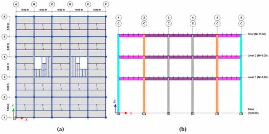
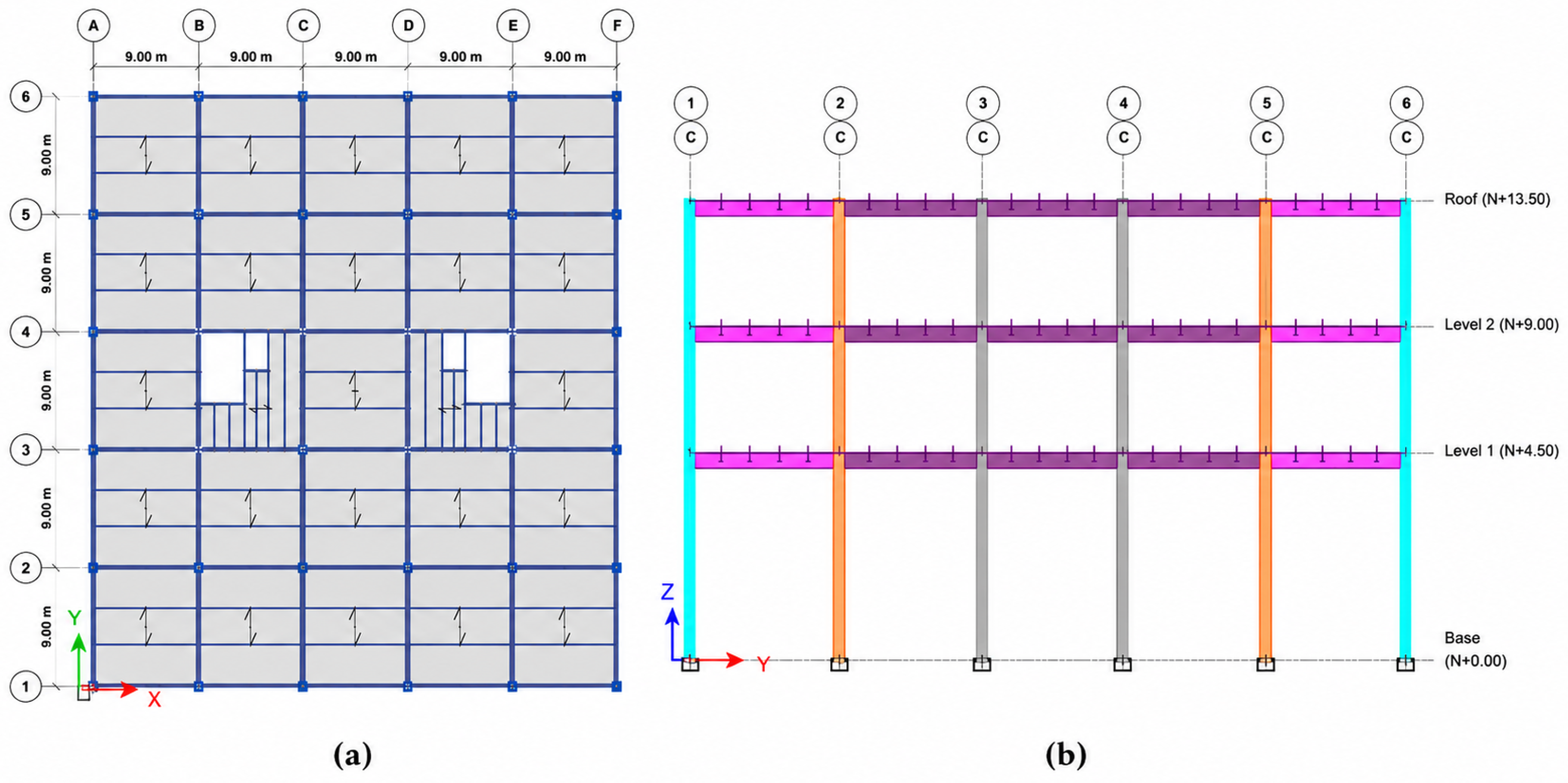
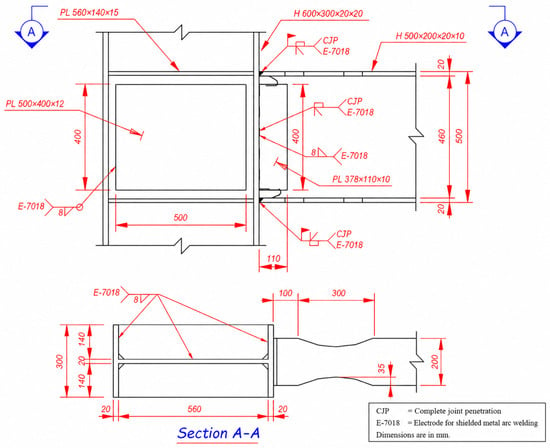
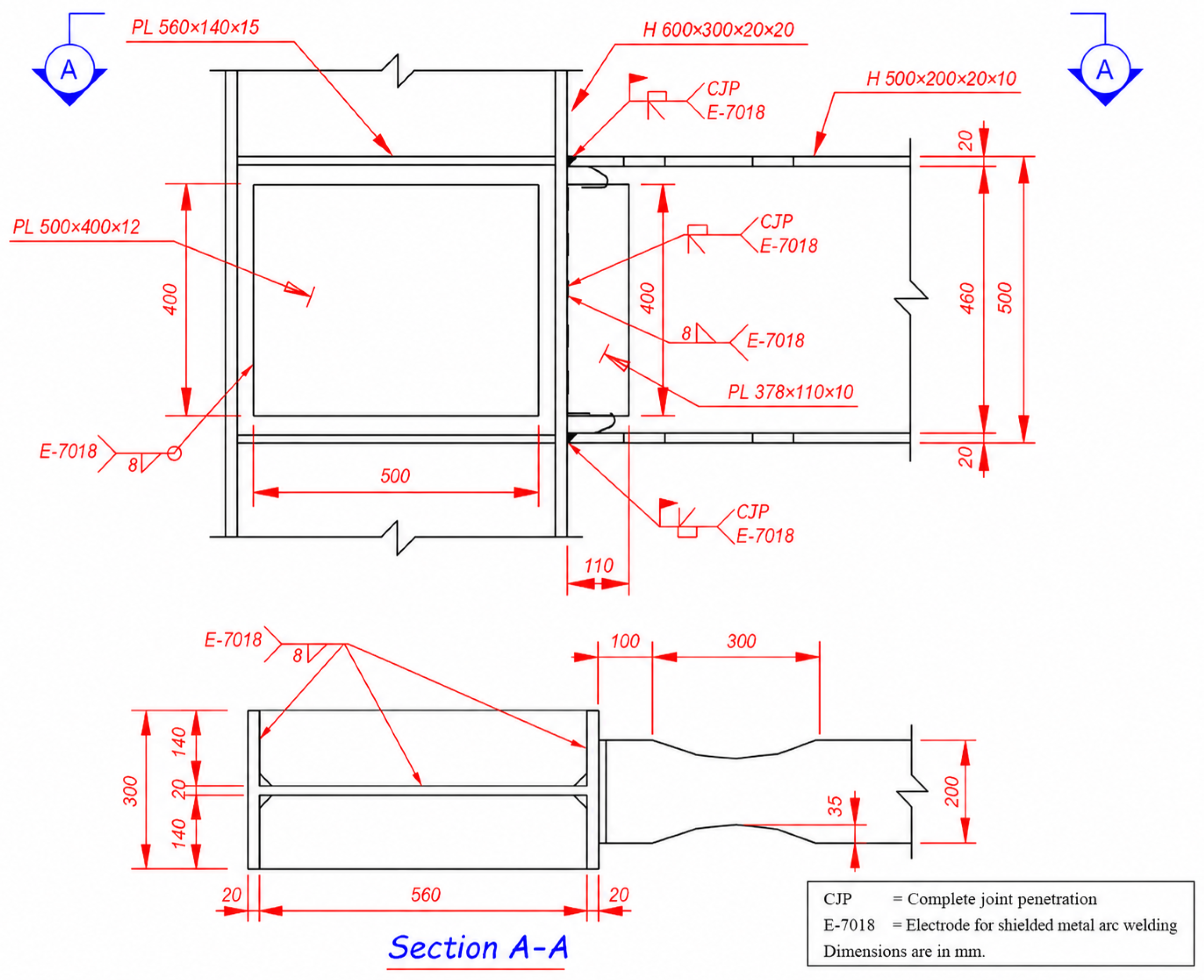
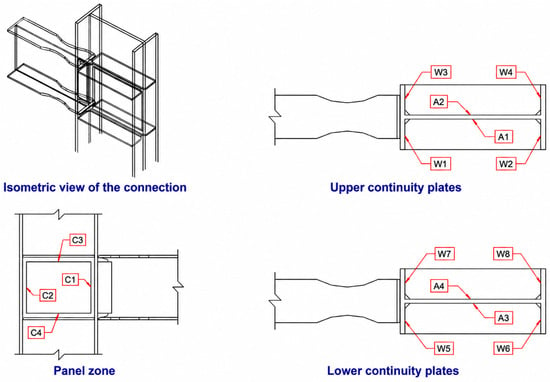
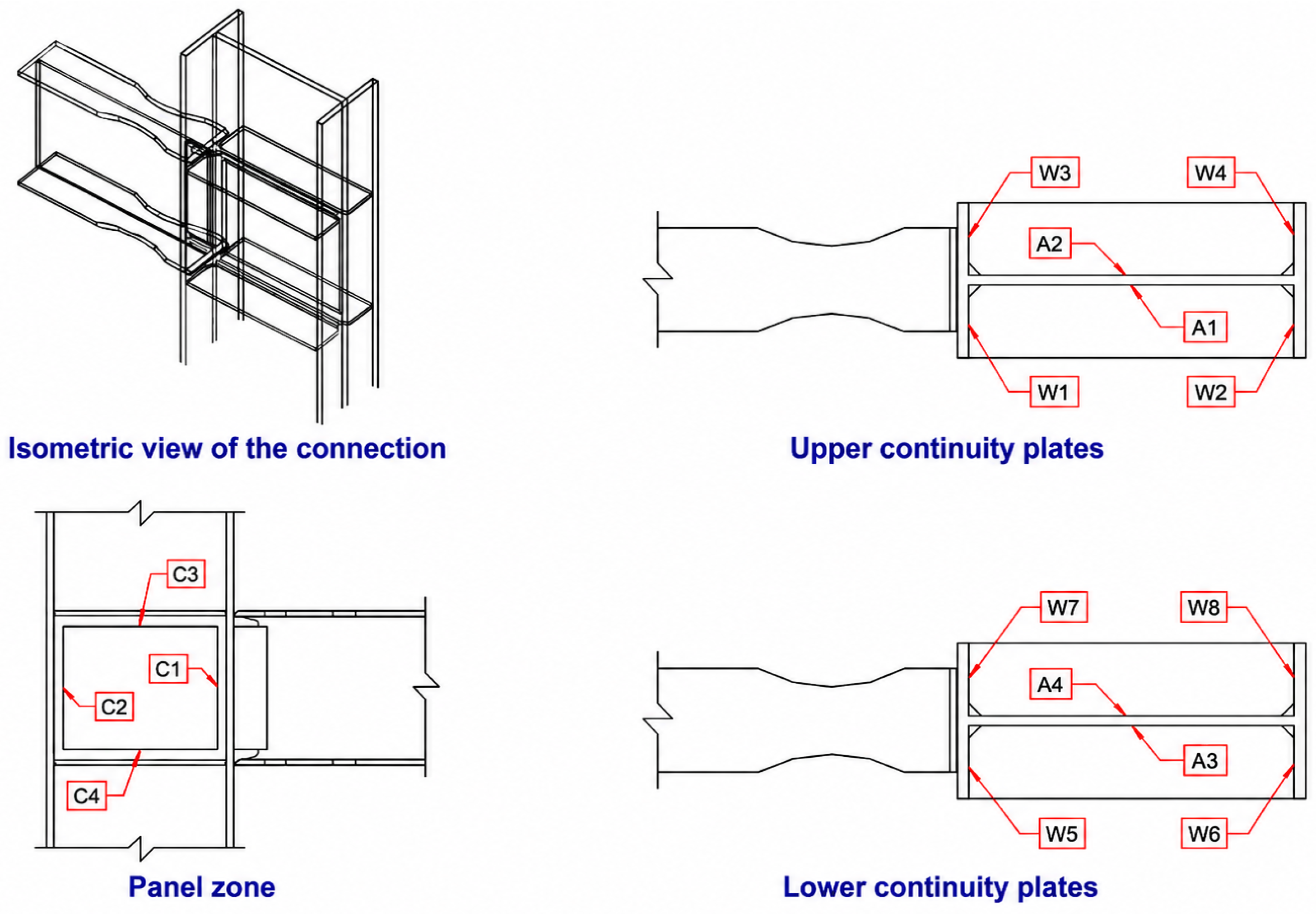
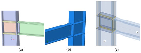
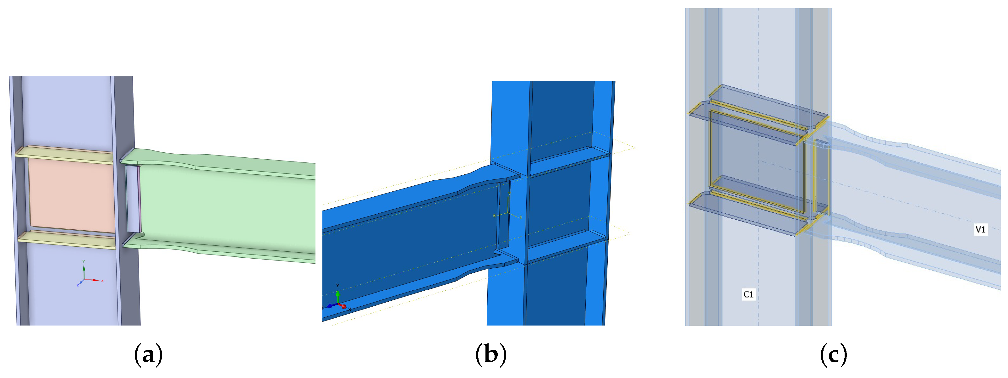
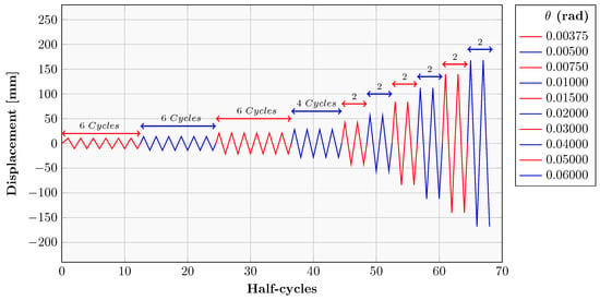
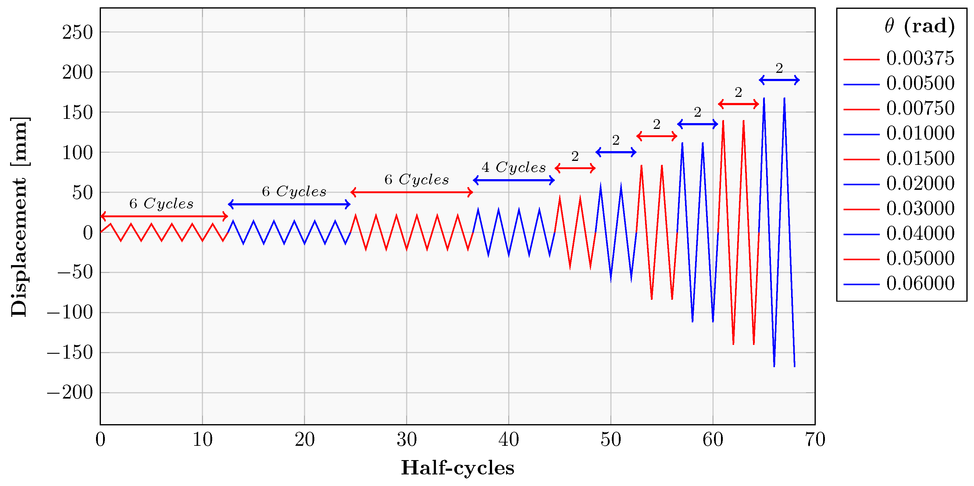
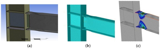
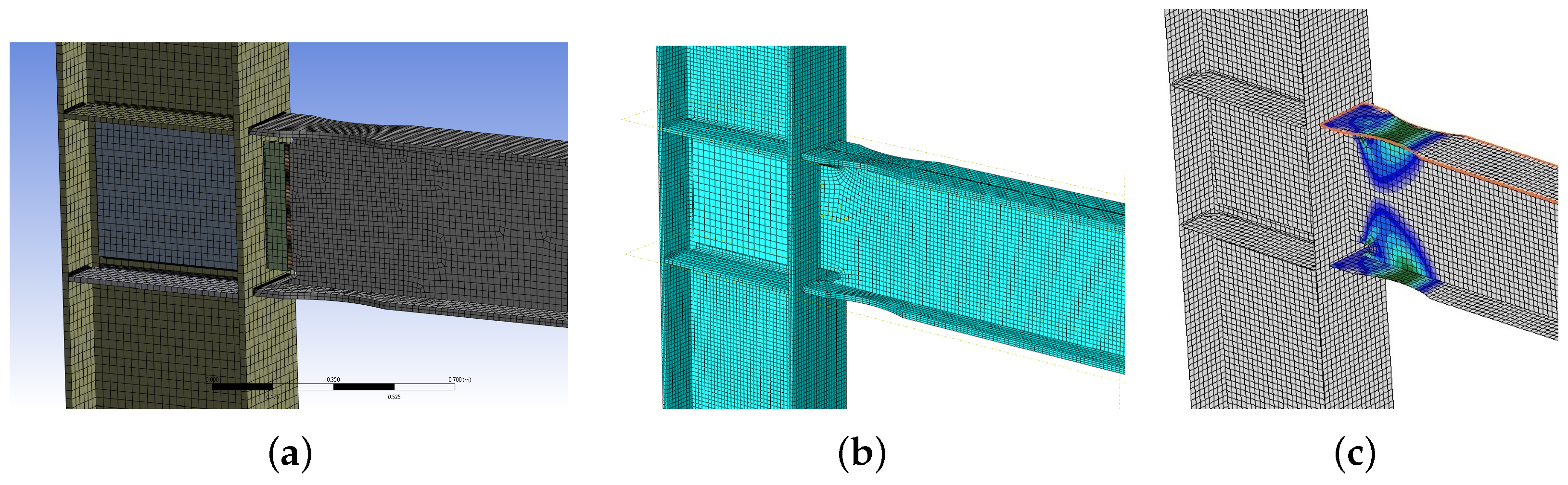
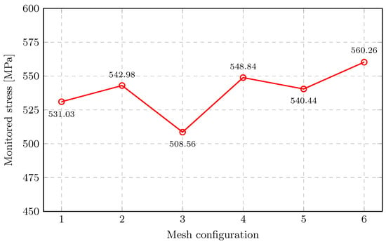
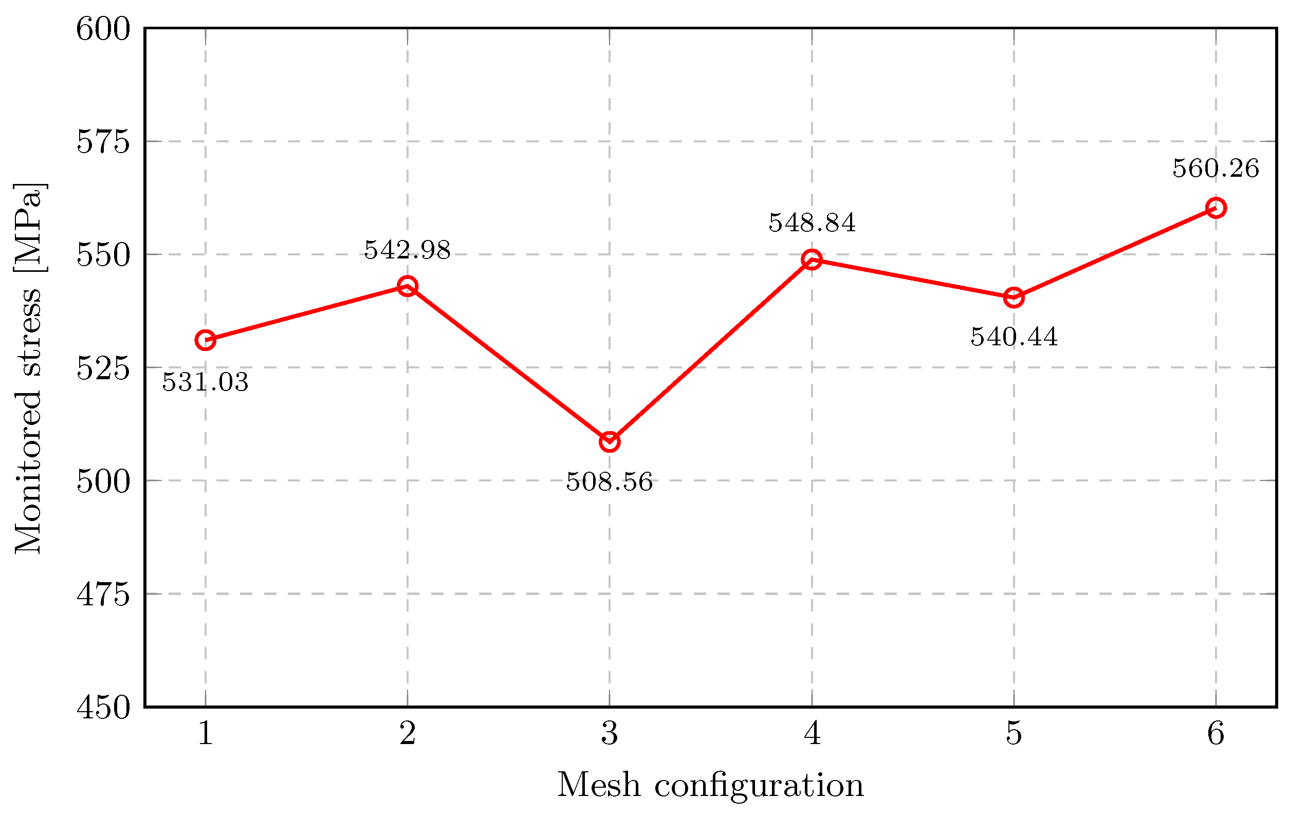
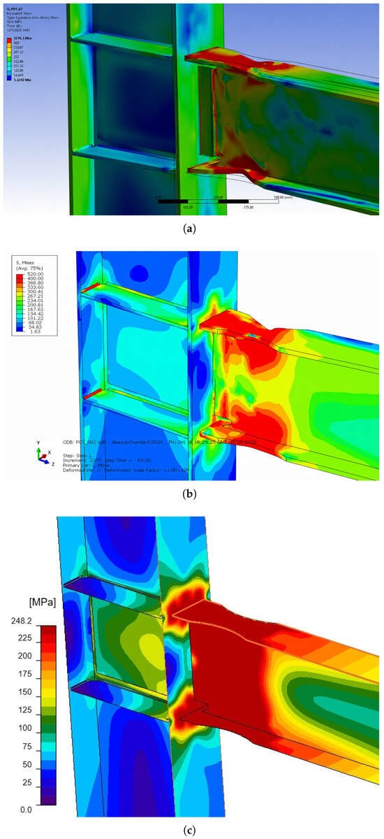
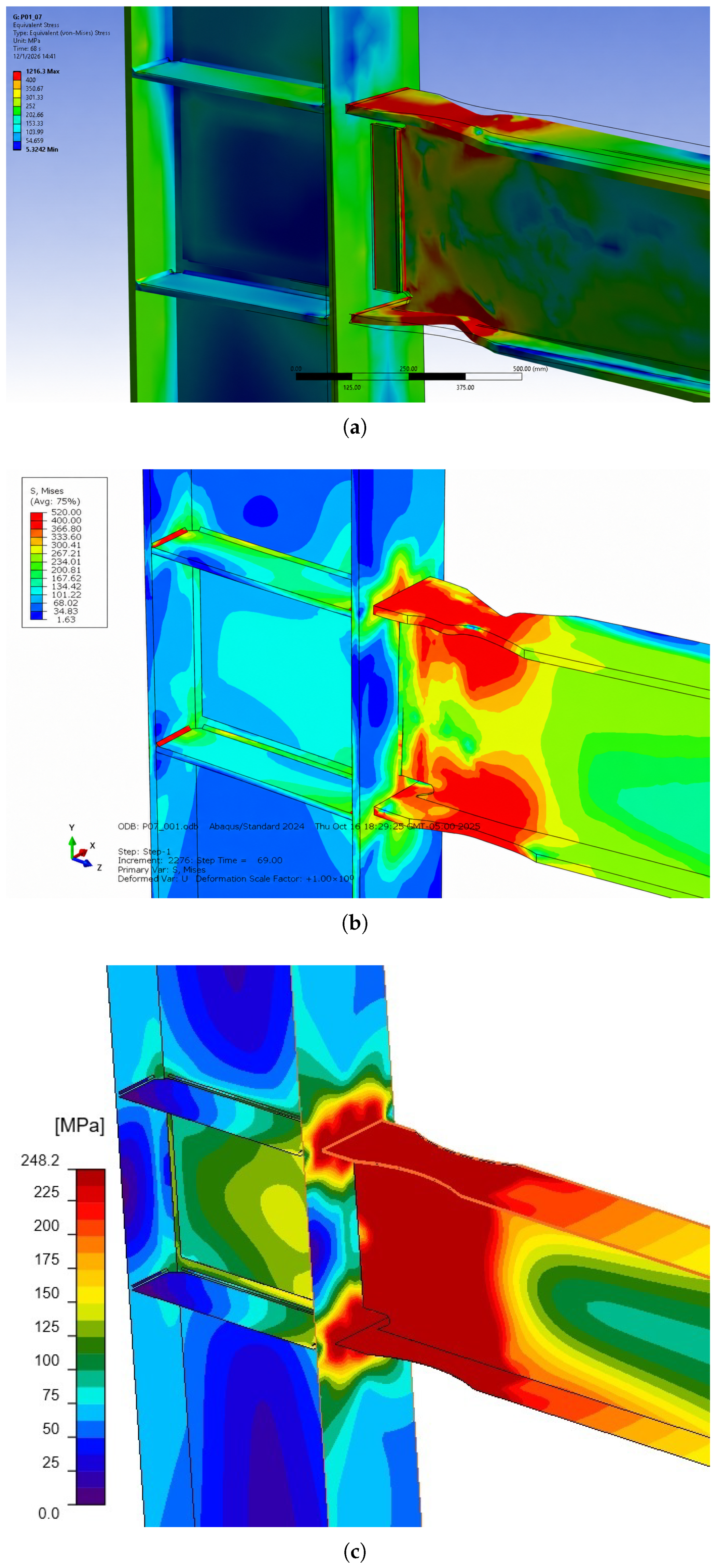
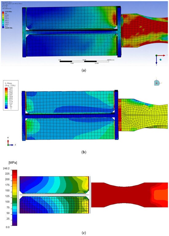
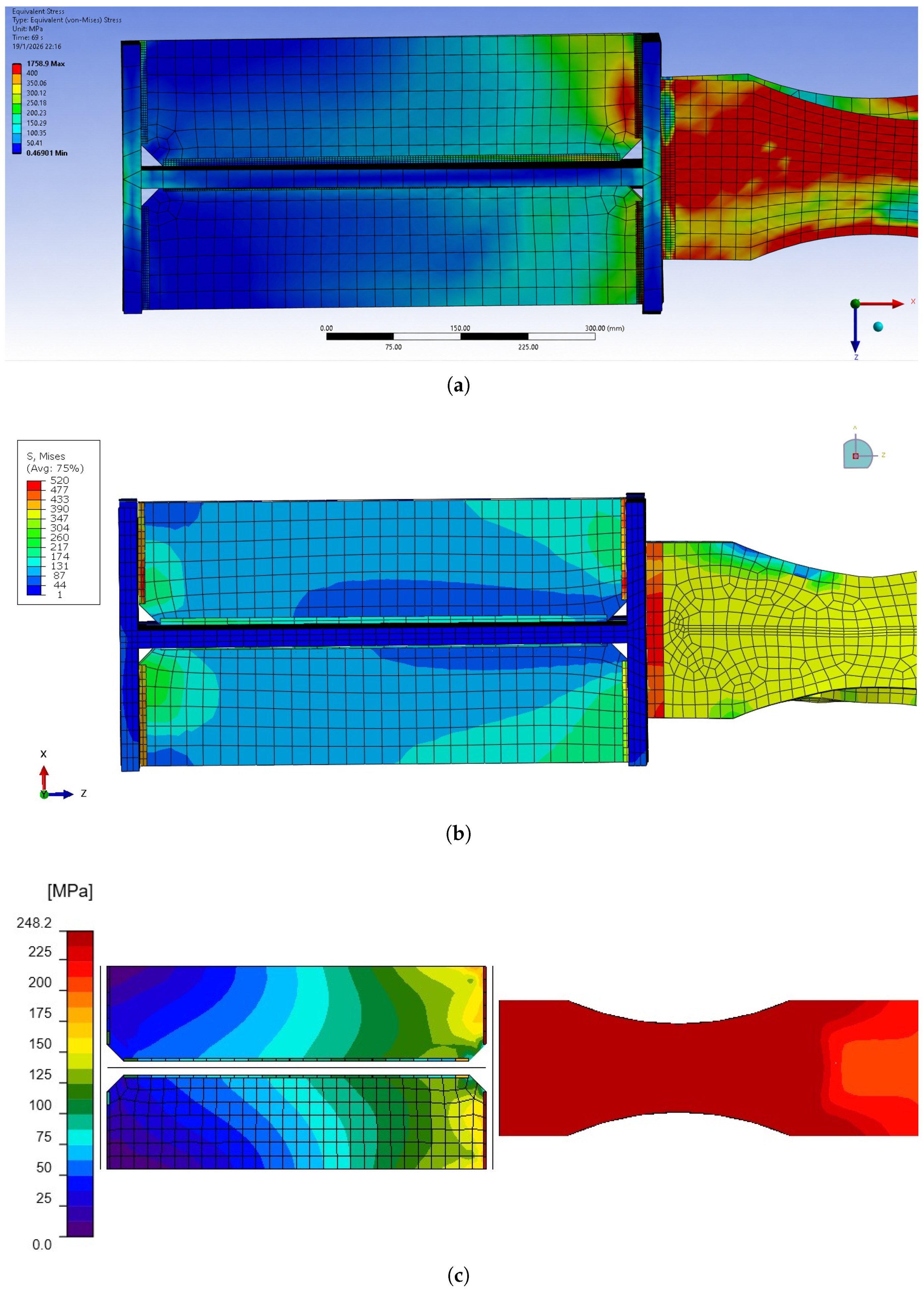
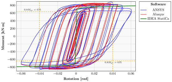
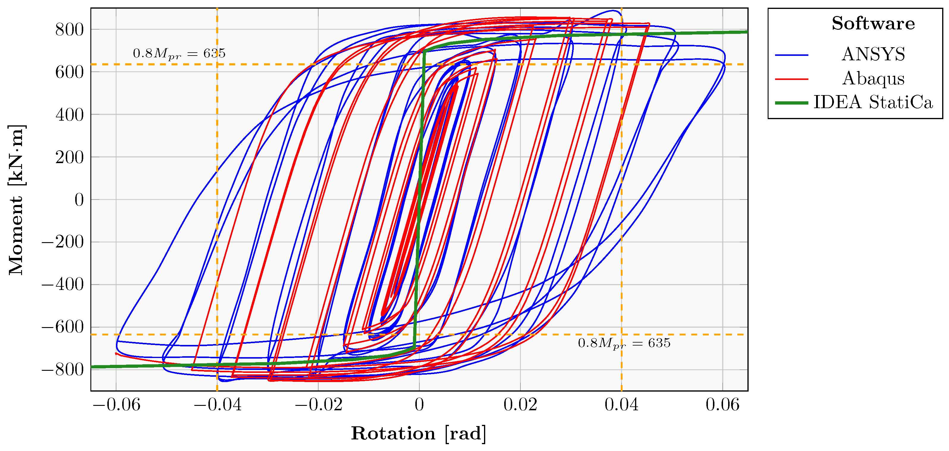
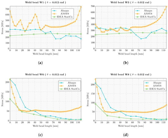
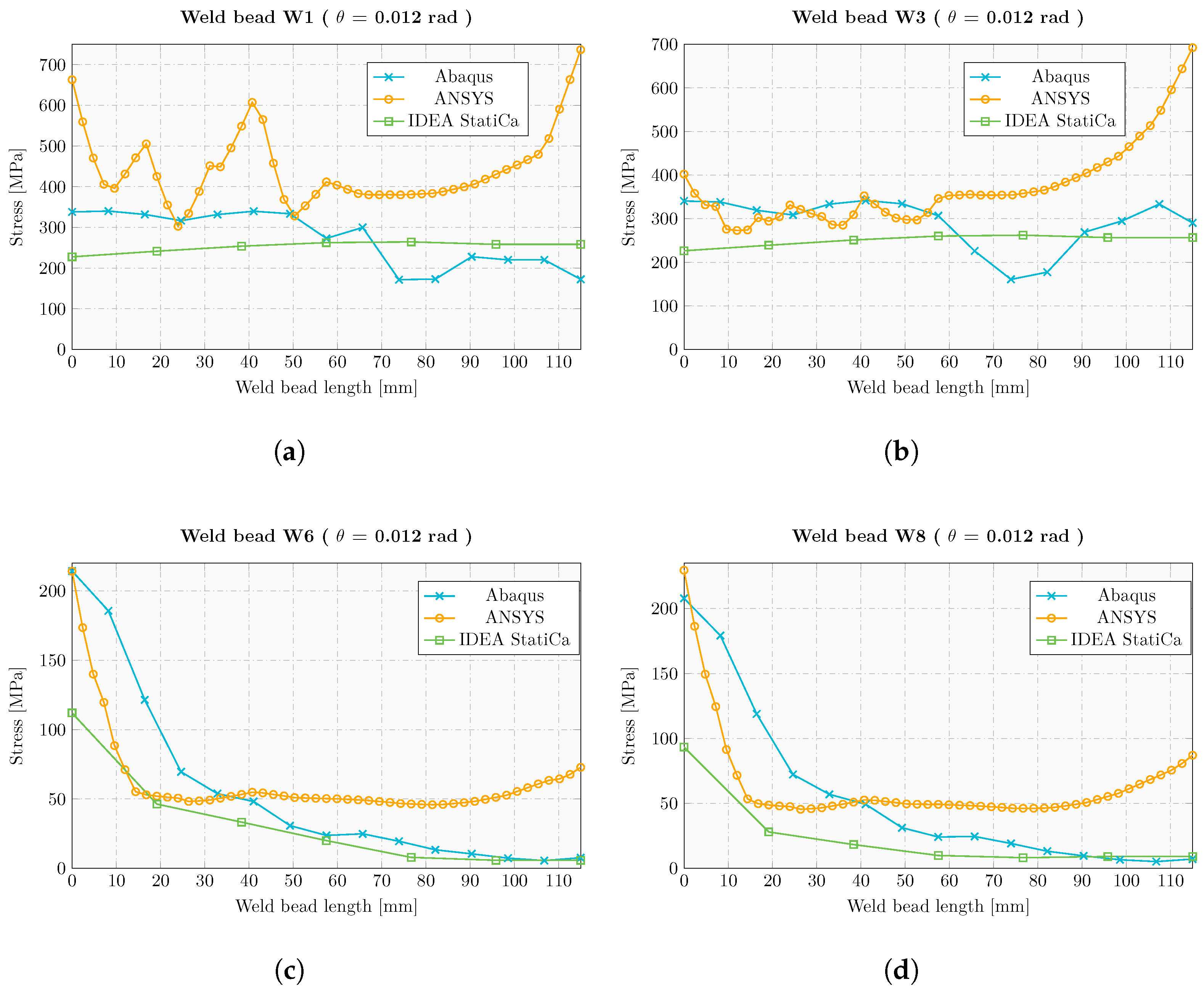
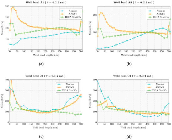
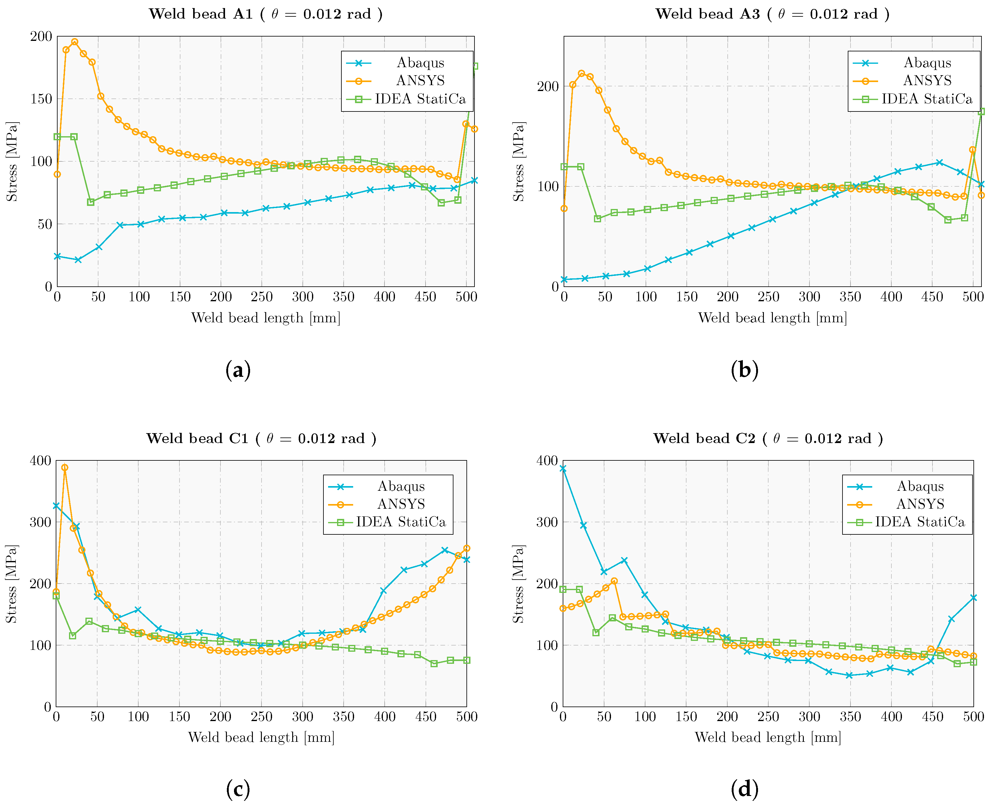

Disclaimer/Publisher’s Note: The statements, opinions and data contained in all publications are solely those of the individual author(s) and contributor(s) and not of MDPI and/or the editor(s). MDPI and/or the editor(s) disclaim responsibility for any injury to people or property resulting from any ideas, methods, instructions or products referred to in the content. |
© 2026 by the authors. Licensee MDPI, Basel, Switzerland. This article is an open access article distributed under the terms and conditions of the Creative Commons Attribution (CC BY) license.