


Abstract
Cold region indoor substations experience persistent high thermal disturbance from electrical equipment, limiting the direct applicability of conventional residential low-carbon strategies. This study couples hourly DeST simulation with partial life-cycle carbon accounting covering A1–A5, B6, C1–C4, Module D, and the greening carbon sink for an operational 110 kV indoor substation in Shijiazhuang. The baseline annual average emission is 59.8 tCO2/year, comprising 21.3 tCO2/year from B6 operational energy and 38.4 tCO2/year from non-B6 contributions. Reducing the roof heat transfer coefficient from 0.50 to 0.20 W/(m2·K) lowers total emissions by 9.4%, followed by the exterior wall at 3.6%, whereas changes in exterior window U-value have negligible influence. Building height reduction yields a theoretical upper bound of 10.7% in the simplified height scan model, but the estimated reduction is only about 3% within the practical 8.0–9.4 m range constrained by equipment clear height requirements. Enhanced interior wall insulation increases emissions by 2.4% and provides no net carbon reduction benefit. Increasing the window-to-wall ratio (WWR) raises emissions for north-, east-, and west-facing facades, while the south-facing response is non-monotonic; among the tested cases, the minimum occurs at WWR = 0.25. These findings provide case-specific quantitative references for passive low-carbon design of high-internal-gain indoor substations in cold regions.
1. Introduction
Under China’s dual-carbon targets and the green transition of power infrastructure, low-carbon building assessment is shifting from a single operational energy consumption metric toward partial life-cycle carbon emission accounting [1], and the dynamic trade-off between operational and embodied carbon has become a central issue in low-carbon design [2]. Recent reviews of carbon footprint accounting methods [3] and of passive building envelope technologies [4] show that both the accounting boundary and the envelope design measures largely determine this trade-off. Cold regions are characterized by long heating seasons and a pronounced conflict between envelope heat loss and internal thermal disturbance. In fully indoor substations, electrical equipment operates around the clock with high thermal disturbance, the intensity of which far exceeds that of typical residential buildings. However, current energy-saving codes and low-carbon design experience have been developed primarily for residential buildings; their direct transplantation to substations readily leads to problems such as insulation redundancy and a surge in cooling load. Therefore, there is an urgent need for quantitative research on partial life-cycle low-carbon design tailored to high-thermal-disturbance indoor substations in cold regions.
Considerable progress has been made regarding partial life-cycle carbon emission accounting methods and their stage-specific characteristics. A relatively complete accounting framework has been established for residential buildings. Fenner et al. [3] reviewed carbon footprint accounting methods and identified system boundary and data quality as the core determinants of cross-study comparability. Kitsopoulou et al. [4] reviewed the passive building envelope technologies that govern both the embodied and the operational carbon of buildings. Yu et al. [5] conducted a BIM-LCA-based accounting for public composite structure buildings and found that embodied carbon in the material manufacturing stage accounts for a significant share. Lin et al. [6] developed an accounting method for prefabricated steel structure office buildings and pointed out that the production and transportation of prefabricated components constitute a critical carbon reduction stage. Röck et al. [2] found that the share of embodied carbon rises as operational energy efficiency improves. Peng [7] calculated a building’s life-cycle carbon emissions based on BIM and Ecotect, while Chastas et al. [8] and Azari et al. [9] reviewed the embodied energy of buildings, and Huang et al. [10] quantified the carbon emissions of the global construction sector. Nevertheless, existing studies have predominantly targeted typical residential buildings, such as dwellings and offices, whereas partial life-cycle accounting for the building envelope of high-thermal-disturbance substations remains markedly understudied.
Passive energy-saving design, which reduces energy consumption and carbon emissions through parametric control of building form and spatial dimensions, envelope heat transfer coefficients, and window-to-wall ratios (WWRs), has been a major research focus. Kitsopoulou et al. [4] reviewed passive building envelope technologies for sustainable design, including envelope-based energy-saving measures. Liu et al. [11] reviewed the impact of urban form on building carbon emissions and showed that form-related parameters such as building shape and layout are important determinants of building-related emissions. Lyu et al. [12] analyzed the life-cycle carbon emissions of buildings with different exterior wall types using BIM, showing that the choice of wall construction measurably affects embodied carbon. Kamel et al. [13] developed a parametric integrated design approach for life-cycle zero-carbon buildings, in which form and envelope parameters are optimized against life-cycle carbon targets. Lim [14] compared reconstruction and renovation schemes and found that renovation yields significant carbon reduction benefits. However, a critical limitation persists: most existing studies employ energy consumption or operational carbon as the sole evaluation indicator, and the dual-stage coupling effect—whereby passive parameters simultaneously influence both embodied and operational carbon—has received insufficient attention.
Research on carbon emissions of power grid buildings, including substations, has been growing. Che et al. [15] reviewed operational-stage carbon emissions of substations and identified the operational phase as the dominant emission source. Wang et al. [16] developed a whole-life-cycle carbon-accounting method for transmission and transformation projects, using a typical 220 kV line and substation as the case. Liu et al. [17] accounted for construction-stage carbon emissions of typical 500 kV transmission and substation projects. Ni et al. [18] investigated integrated design optimization of modular substations under zero-carbon targets. Gu et al. [19] analyzed green and low-carbon technology pathways for substations in new-type power systems. However, these studies have largely focused on electrical equipment and whole-process accounting, and the interactive relationship between passive design elements of the substation building envelope—namely, building form, envelope performance, and orientation-specific window openings—and carbon emissions within the partial life-cycle boundary lacks quantitative investigation.
Taken together, three gaps remain in the existing literature. First, the adaptability of research objects is insufficient: carbon accounting and trade-off models have been developed mainly for residential and office buildings [5,6,12], whereas substation studies have focused on electrical equipment and whole-process accounting [15,16,17]; neither can readily accommodate the load profile of a substation building characterized by persistent high thermal disturbance. Second, research perspectives are fragmented: most studies account for embodied carbon or operational carbon in isolation [4,9,12], and a parametric design approach against whole-life carbon targets has so far been proposed only for generic building types [13]; the coupling of passive design parameters with both carbon stages has, therefore, not been quantified. Third, practical implementation support is weak: existing substation studies provide technology roadmaps and single-objective optimizations [18,19], but integrated optimal value ranges for building form, envelope performance, and WWR for indoor substations in the cold climate of North China remain unexplored, leaving design selection without a quantitative basis.
Addressing these gaps, this study takes an operational 110 kV fully indoor, staffed substation in Yuhua District, Shijiazhuang, as the research object. The DeST energy simulation tool [20] is employed to construct an annual hourly dynamic simulation model for cooling and heating loads. The accounting boundary is defined with reference to the accounting frameworks established by the Standard for Building Carbon Emission Calculation (GB/T 51366-2019) and ISO 14040 [21]. The control variable method is adopted to quantify the coupling effects of building height, envelope heat transfer coefficients, and orientation-specific WWRs on carbon emissions from both the material manufacturing stage and the 50-year operational stage. This study quantifies the actual carbon benefits of conventional energy-saving measures, such as interior wall insulation and story height control, distinguishes net carbon-reducing measures from carbon-increasing risk measures, and proposes integrated optimal value ranges for substation building form, envelope performance, and WWR adapted to the cold climate of North China, thereby providing a quantitative basis for low-carbon design of similar substations. Compared with existing residential building studies, the marginal contribution of this work lies in extending the partial life-cycle carbon accounting framework to industrial buildings with persistently high thermal disturbance from equipment, systematically quantifying the dual-stage coupling effects of passive parameters on material manufacturing carbon and operational carbon, and uncovering patterns that diverge from residential building design experience—including net carbon increase from thermal enhancement of interior walls, north and east window openings being most unfavorable, and roof insulation being the priority envelope measure.
2. Model Establishment
The research object of this study is a 110 kV fully indoor, staffed substation located in Yuhua District, Shijiazhuang, Hebei Province (Figure 1). The building has a well-defined functional layout, comprising a main transformer room, main transformer capacitor room, 10 kV power distribution room, 110 kV gas-insulated switchgear (GIS) room, secondary equipment room, battery room, pump room, safety tool room, records room, and ancillary facilities. As a typical indoor substation in cold regions, the building features a regular floor plan, and its equipment arrangement and spatial form are generally consistent with those of similar substations newly constructed in recent years, which gives the findings regional reference value. The building is a single-story (one story above ground), frame structure indoor substation with a total floor area of 1181.81 m2 and an external surface area of 2088.50 m2; its building volume is 3545.43 m3, and the shape coefficient is 0.59. The building has an approximately rectangular plan of about 40.5 m × 28.8 m (axis dimensions), corresponding to a plan aspect ratio of about 1.4:1. The plan is regular with a local recess, and the functional rooms are arranged around the main equipment hall.
Figure 1.
Location of the studied 110 kV indoor substation in Shijiazhuang, Hebei Province, China.
2.1. DeST Energy Consumption Model
DeST [20] is employed to establish an annual hourly dynamic simulation model of the 110 kV fully indoor, staffed substation in Yuhua District, Shijiazhuang. The building geometry and functional zones are reconstructed from the construction drawings, and the typical meteorological year hourly data for Shijiazhuang and the equipment thermal disturbance compiled from the equipment nameplate data and the design documents are imported into the model. The hourly cooling and heating loads for the full year of 8760 h are then solved, providing the energy consumption input for partial life-cycle carbon emission accounting. The complete set of simulation input parameters is listed in Table S3 of the Supplementary Materials. The functional layout of the studied substation is shown in Figure 2.
Figure 2.
Schematic of the functional layout of the studied substation building (not to scale).
- (1)
- Meteorological input parameters. Shijiazhuang is located in a cold region, and the outdoor design parameters are determined in accordance with the Code for Design of Heating, Ventilation and Air Conditioning of Civil Buildings (GB 50736-2012) [22]. The heating period is set to 121 days based on the actual heating supply cycle. The simulation adopts the typical meteorological year hourly data for Shijiazhuang, and the main parameters are listed in Table 1 [22].Table 1. Meteorological input parameters for Shijiazhuang.
- (2)
- Building envelope construction. All construction layers were included in the U-value calculation, including the 20 mm cement mortar layers, the concrete block, and the 120 mm reinforced concrete roof slab. The thermal conductivities adopted were 0.93 W/(m·K) for cement mortar, 0.58 W/(m·K) for the concrete block, 0.18 W/(m·K) for aerated concrete, 1.74 W/(m·K) for reinforced concrete, and 0.030 W/(m·K) for extruded polystyrene; these values were taken from the thermal design code for civil buildings and manufacturer data [23]. The construction layers and heat transfer coefficients of the building envelope are listed in Table 2. A thermal model is established layer by layer according to the actual construction, and on this basis, the heat transfer coefficients of each component are adjusted in gradients in Section 3.Table 2. Construction layers and heat transfer coefficients of the substation building envelope.
- (3)
- Indoor thermal disturbance and air conditioning boundary. The electrical equipment in the substation operates continuously around the clock with high heat dissipation, representing a typical high internal thermal disturbance condition. Based on the equipment nameplate data and the design documents, the rated power, operating power, and operating schedule of each equipment item were used to define the internal heat gains of the corresponding functional rooms. The equipment parameters and schedule assumptions are summarized in Table 3 and Table S5 of the Supplementary Materials. The indoor space is only periodically inspected, and split air conditioners are adopted (cooling seasonal energy efficiency ratio [SEER] = 3.60, heating seasonal performance factor [HSPF] = 2.60), with a temperature control range of 20–28 °C. The model structure and the operational assumptions adopted in this study follow the published DeST-based study of the same station [24], including the treatment of the air-conditioning system, the neglect of mechanical ventilation and infiltration, and the assumption that doors remain closed except during the one or two weekly inspection tours. The thermal disturbance input remains consistent across all scanning scenarios, and its seasonal fluctuations do not affect the conclusions of the relative comparisons. Mechanical ventilation and infiltration were not explicitly included in the model: no fresh air or air change rate was specified as a simulation input, and the rooms are served by split air conditioners only. This simplification is acknowledged as a source of uncertainty.Table 3. Room and equipment parameters of the substation.
- (4)
- Model construction, solution, and input verification. The building geometry is established based on the construction drawings. After importing the typical meteorological year data, DeST solves the annual hourly cooling and heating loads of the building under the specified internal disturbance conditions, which provide the operational load profile of the scheme. The operational-stage energy consumption used in the carbon accounting (cooling, heating, lighting, the elevator, and domestic hot water) is obtained from the building energy calculation of the compliance module, giving 24,134 kWh/year in the baseline case. The model verification focuses on the traceability of input parameters and the self-consistency of calculation logic [25]. It should be emphasized that this is an input data and model consistency verification rather than a measured data calibration because project-specific submetered HVAC energy consumption data of the substation were not available. The simulation results are primarily used for the relative comparison of design schemes and the analysis of emission reduction patterns under a unified baseline scenario.
- (5)
- Parameter scanning scenarios. A control variable method is adopted, in which only one parameter is changed at a time while the rest remain at baseline values. The envelope heat transfer coefficients of the baseline scenario follow Table 2 (exterior wall 0.50, interior wall 0.96, roof 0.50, exterior window 1.8 W/(m2·K)). The scanning ranges are: building height 4.3–9.4 m; roof and exterior wall heat transfer coefficients 0.20–0.50 W/(m2·K); interior wall heat transfer coefficient 0.60–1.20 W/(m2·K); exterior window heat transfer coefficient 1.8–3.0 W/(m2·K); and orientation-specific WWRs of 0.05–0.50. For each scenario, the annual average carbon emissions (tCO2/year) of the non-B6 stages, the operation stage (B6), and the partial life-cycle are reported. No single baseline WWR was used for the WWR scan: each orientation was varied parametrically from 0.05 to 0.50. In all other single-parameter scans, the WWR of each orientation was held constant at the as-built value, so that the control variable comparison is preserved.
2.2. Partial Life-Cycle Carbon Accounting Framework
The life-cycle assessment (LCA) method accounts for environmental emissions of building products throughout the process from raw material acquisition to final disposal, following the principle framework established by ISO 14040/14044 [21,26]. Methods and frameworks for building partial life-cycle carbon emission accounting have been systematically studied [1,27]. In accordance with the Standard for Building Carbon Emission Calculation (GB/T 51366-2019) and the EN 15978 module system [28], this study divides the life-cycle into the product and construction stage (A), use stage (B), end-of-life stage (C), and benefits from recycling and reuse (D). The definitions and inclusion status of each module are listed in Table 4.
Table 4.
Building stage division and accounting boundary.
The functional unit of this study is the substation building itself with a design service life of 50 years. The accounting covers the modules resolved by the carbon-accounting model: material production and transport (A1–A4), construction and installation (A5), operational energy use (B6, including the 50-year heating, cooling, ventilation, lighting, elevator, and domestic hot water energy), demolition and disposal (C1–C4), recycling benefits (D), and the greening carbon sink. Use, maintenance, repair, replacement, refurbishment, and operational water use (B1–B5, B7) are not resolved by the model. To unify the time basis, the non-B6 emissions are amortized over 50 years and included in the annual average carbon emissions. The operational stage is accounted for on an annual basis, and its 50-year cumulative value is included in the total partial life-cycle carbon accounting. Related studies have also pointed out that the accounting boundary and data quality are key determinants of the international comparability of building carbon accounting [29].
Within the accounting model adopted in this study, the modules that are not resolved are use, maintenance, repair, replacement, refurbishment, and operational water use (B1–B5, B7); the remaining modules reported by the model are all included, as listed in Table 4. These unresolved modules depend on project-specific operation and maintenance records that were not available for the studied station, and some of them may vary with the investigated passive design parameters (for example, insulation thickness, facade material quantities, and window area may influence replacement and end-of-life emissions). Their influence on the reported shares and on the parameter ranking is, therefore, treated as a source of uncertainty rather than assumed to be negligible, and it is examined through the exploratory sensitivity scenarios applied below and the replacement case in Section 3.5. The high-voltage electrical equipment in the substation is independent of the building envelope system and does not fall within the scope of the building itself, although its heat dissipation is included in the operational simulation as internal thermal disturbance. The term “partial life-cycle carbon emissions” in this study, therefore, refers exclusively to results within the boundary defined above, and the relevant conclusions hold only within this boundary.
It should be noted that GB/T 51366-2019 was developed for carbon emission accounting of civil buildings, whereas substations fall into the category of industrial buildings. This study, therefore, adopts only its accounting framework and emission factor database, with the system boundary defined as follows: (i) only the building itself is included in the carbon inventory; the electrical equipment inside the substation is excluded, although its heat dissipation is incorporated into the operational energy simulation as internal thermal disturbance; (ii) because the substation operates under persistently high internal thermal disturbance, the ventilation and air-conditioning boundary conditions were determined with reference to GB 50019-2015 [30] (Code for Design of Heating, Ventilation and Air Conditioning for Industrial Buildings) and DL/T 5218-2012 [31] (Technical Code for Design of 220 kV–750 kV Substations); and (iii) the material and energy carbon emission factors of GB/T 51366-2019 can be directly reused because they are material- or energy-specific rather than building type-specific.
Terminology and boundary: In this study, “partial life-cycle carbon emission” refers to the carbon emissions of all life-cycle modules reported by the carbon-accounting model, namely, material production and transport (A1–A4), construction and installation (A5), operational energy use (B6, covering heating, cooling, ventilation, lighting, the elevator, and domestic hot water), demolition and disposal (C1–C4), recycling benefits (D), and the greening carbon sink. For clarity, the combined contribution of A1–A5, C1–C4, Module D, and the greening carbon sink is hereafter referred to as the non-B6 contribution (referred to as non-B6 carbon in the figures), whereas the operational energy contribution is represented by B6. Use, maintenance, repair, replacement, refurbishment, and operational water use (B1–B5 and B7) are not resolved by the model; the replacement module (B4) is, therefore, added separately as a sensitivity case in Section 3.5. The baseline assessment, therefore, includes A1–A5, B6, C1–C4, Module D, and the greening carbon sink, while B1–B5 and B7 are excluded; B4 is additionally examined as a supplementary sensitivity module. The stage-by-stage composition of the assessed total is reported in Table S6 of the Supplementary Materials.
Because these modules are not resolved by the model, their influence is examined through exploratory sensitivity scenarios rather than simulated: the maintenance- and replacement-related modules (B2–B5, i.e., maintenance, repair, replacement, and refurbishment) are covered by the +/−10% and +/−20% perturbation applied below and by the explicit B4 replacement case in Section 3.5, whereas operational water use (B7) concerns water consumption itself, with the energy for heating it being already included in B6. Sartori and Hestnes [32] reviewed life-cycle energy studies and reported that the operational stage accounts for about 80–90% of the life-cycle energy of conventional buildings, with embodied energy contributing 10–20%. Chau et al. [33] reviewed building LCA/LCEA/LCCO2 studies and found that transport, construction, demolition, and disposal generally represent a small share of the total, although the reported values depend strongly on the system boundary. Dixit et al. [34] further showed that embodied energy estimates vary widely with boundary definitions and data sources, and that transport and construction are frequently excluded or only partially included. The cradle-to-grave UK case studies of Moncaster and Symons [27] indicated that material production dominates the embodied share, whereas transport, construction, and demolition/disposal are comparatively minor; Cabeza et al. [35] and Chastas et al. [8] reached similar conclusions for the building sector, while noting that maintenance and replacement can become significant when component service lives are shorter than the building life.
To test the influence of the modules that the model does not resolve, and of the uncertainty in the embodied carbon data, a uniform perturbation of +10% and +20% was applied to the embodied carbon of all scenarios; this perturbation is used as a robustness test rather than as a quantified bound for the unresolved modules. The total carbon increases from 59.8 to 63.6 tCO2/year (+6.4%) and 67.4 tCO2/year (+12.9%), respectively, but the qualitative conclusions remain unchanged: roof insulation produces the largest reduction (9.4%), followed by exterior wall insulation (3.6%); changing the exterior window U-value has a negligible effect, whereas enhanced interior wall insulation increases total carbon emissions by approximately 2.4%. Adding the B4 replacement module (Section 3.5) increases the assessed total by at most about 0.55 tCO2/year (0.9%). In the same way, to bound the influence of the operational input assumptions, the operation-stage (B6) carbon was perturbed by ±20%: the assessed total then ranges from 55.5 to 64.0 tCO2/year (about ±7% around the baseline), the operational share ranges from 31% to 40%, and the ranking of the passive measures remains unchanged (roof insulation 8.2–10.7%, exterior wall insulation 3.2–4.1%, external windows approximately 0%, and interior wall insulation a net increase) because the measure-specific operational savings scale approximately with the operational carbon.
Across these cases, the baseline non-B6/B6 split remains within approximately 60–69% (operation 31–40%). Within the tested exploratory sensitivity scenarios, the non-B6 contribution remained larger than the B6 operational contribution. We, therefore, report this split only within the adopted partial life-cycle boundary and explicitly retain the unresolved B-stage modules as a source of uncertainty rather than assuming that their effects are negligible.
Boundary composition and conservative boundary sensitivity scenario: The stage-by-stage composition of the assessed total is material production and transport (A1–A4) 38.91, construction and installation (A5) 0.67, operational energy (B6) 21.34, demolition and disposal (C1–C4) 0.11, recycling benefits (D) −0.91, and the greening carbon sink −0.35 tCO2/year (Table S6), giving a baseline total of 59.77 tCO2/year (rounded to 59.8 tCO2/year at three significant figures); this is the full set of modules resolved by the carbon-accounting model, so all the modules it resolves are included. Because the transport, construction, demolition, and recycling terms in the model are computed from the baseline material quantities, deliberately conservative upper-bound allowances were additionally applied to the additional material introduced by each passive measure: 500 km transportation, construction equal to 5% of material carbon, one replacement within 50 years, and end-of-life equal to 2% of material carbon with no recycling credit. Even under these assumptions, the net reduction in the roof measure remains above about 4.5 tCO2/year and that of the exterior wall measure above about 1.5 tCO2/year; interior wall insulation becomes more carbon intensive and external windows remain negligible. The ranking of the passive measures is, therefore, unchanged under these conservative boundary assumptions.
The baseline scenario is defined as follows: building height follows the as-built condition in the construction drawings; envelope heat transfer coefficients follow Table 2 (exterior wall 0.50, interior wall 0.96, roof 0.50, exterior window 1.8 W/(m2·K)); the window-to-wall ratio is treated as a parametric variable and scanned from 0.05 to 0.50 for each orientation (Section 3.4), while in all other single-parameter scans, the WWR of each orientation is held constant at its as-built value; the heating period is 121 days; equipment heat dissipation is converted from the equipment nameplate data and the design documents; split air conditioners are adopted; and the electricity carbon emission factor is taken as 0.8843 kgCO2/kWh for the North China regional power grid. Except for the parameter under investigation, all scanning scenarios maintain this baseline unchanged.
It should be noted that the YJK (Yingjianke) model reports annual average carbon emissions for all the life-cycle modules it resolves (A1–A5, B6, C1–C4, D, and the greening carbon sink), and that this module set is adopted in the present study (Table 4). The only modules that the model does not resolve are use, maintenance, repair, replacement, refurbishment, and operational water use (B1–B5, B7), whose influence is examined through exploratory sensitivity scenarios rather than simulated, as described in Section 2.2 and Section 3.5. The influence of these unresolved modules on the parameter ranking is, therefore, treated as a source of uncertainty rather than assumed to be negligible.
Accordingly, the total partial life-cycle carbon emissions consist of the combined 50-year non-B6 contribution and the 50-year cumulative operational carbon [36]. To facilitate cross-comparison, this study uniformly adopts an annualized conversion basis: the annualized carbon emissions of the non-B6 stages equal the combined 50-year non-B6 contribution divided by 50, while the annual carbon emissions of the operational stage serve directly as the annual average; the sum of the two constitutes the total annualized carbon emissions within the partial life-cycle boundary. The calculation models are presented in Section 2.4 and Section 2.5. In this paper, the unit tCO2/year denotes tons of CO2 equivalent per year.
2.3. Carbon Emission Factors and Calculation Parameters
Carbon emission factors are key parameters in carbon emission accounting, and their adopted values directly affect the accuracy and comparability of accounting results. In this study, the material manufacturing carbon emission factors are selected based on Appendix D of the Standard for Building Carbon Emission Calculation (GB/T 51366-2019) [37] and authoritative industry carbon emission databases. The electricity carbon emission factor is taken as the North China regional power grid emission factor (0.8843 kgCO2/kWh, obtained from the built-in carbon emission database of YJK Green Building Design Software V2025 (r1.0)). The carbon emission factor for heat is taken as the regional district heating average value from Appendix D of GB/T 51366-2019 (0.11 tCO2/GJ). The main carbon emission factors and their sources are listed in Table 5 and, in tabular form, in Table S2 of the Supplementary Materials.
Table 5.
Main carbon emission factors and sources.
The main accounting of this study is conducted on a conservative basis with the baseline-year electricity carbon emission factor (0.8843 kgCO2/kWh) held constant. Existing studies have shown that provincial power grid carbon emission factors in China exhibit a year-by-year declining trend [38,39]. The long-term impact of grid decarbonization on operational carbon emissions is quantified by the scenario analysis in Section 3.5; the evolution of the grid factor beyond those scenarios is left for future work.
The material quantities are calculated based on the construction drawings and actual construction practices, consistent with the energy consumption model inputs in Section 2.1. The products of the material quantity and the corresponding carbon emission factor of each component are summed item by item according to Equation (1) in Section 2.4, yielding the one-time carbon emissions of the material manufacturing stage (A1–A3). For the baseline scenario, this A1–A3 contribution is 1865.93 tCO2, i.e., 37.32 tCO2/year when annualized over the 50-year design service life. Adding transport (A4), construction and installation (A5), demolition and disposal (C1–C4), recycling benefits (D), and the greening carbon sink gives the non-B6 contribution, which totals approximately 1921 tCO2 (38.4 tCO2/year). The detailed material inventory and the corresponding carbon emission values are provided in Table S1 of the Supplementary Materials. It should be noted that for a few materials the reported carbon emission values and the product of quantity × production factor differ in the source inventory; the values adopted in the material manufacturing (A1–A3) accounting of this study are the reported carbon emission values of the inventory, and the production factor column is provided for reference only.
2.4. Partial Life-Cycle Carbon Accounting Method
(1) Embodied Carbon Emissions from the Material Manufacturing Stage
is the total one-time embodied carbon emissions from the material manufacturing stage, tCO2; this value is amortized over the 50-year design service life to obtain the annualized value.
is the quantity of the i-th building material, t (or m3, m2, corresponding to the unit of the carbon emission factor).
is the carbon emission factor for manufacturing the i-th building material, tCO2 per unit quantity.
is the total number of building material types.
(2) Annual Carbon Emissions from the Building Operational Stage
is the carbon emissions from the building operational stage in the y-th year, tCO2/year.
is the total electricity consumption for heating, cooling, ventilation, etc., in the y-th year, kWh.
is the carbon emission factor of the regional power grid, tCO2/kWh (0.8843 kgCO2/kWh = 8.843 × 10⁻⁴ tCO2/kWh).
is heat consumption from district heating in the y-th year, GJ (taken as 0 when no district heating is supplied for this project).
is the heat carbon emission factor, tCO2/GJ.
(3) Total Carbon Emissions
is the total carbon emissions within the partial life-cycle boundary over 50 years, tCO2.
is the total one-time embodied carbon emissions from the material manufacturing stage, tCO2; this value is amortized over the 50-year design service life to obtain the annualized value.
is the cumulative operational carbon emissions over 50 years, tCO2.
(4) Annualized Carbon Emissions
is the annualized carbon emissions within the partial life-cycle boundary, tCO2/year.
2.5. Evaluation Indicators
2.5.1. Carbon Emission Intensity per Unit Floor Area
is building floor area, m2.
is cumulative carbon intensity within the partial life-cycle boundary per unit floor area, kgCO2/m2.
is the annual average carbon intensity per unit floor area for the operational stage, kgCO2/(m2·year).
is the annual carbon emissions from the operational stage, tCO2/year.
is the annualized carbon intensity within the partial life-cycle boundary per unit floor area, kgCO2/(m2·year).
2.5.2. Carbon Emission Reduction Rate
is the reduction rate of total carbon emissions within the partial life-cycle boundary, %.
is the total carbon emissions of the baseline scenario within the partial life-cycle boundary, tCO2/year (annual average basis).
is the total carbon emissions of the optimized scenario within the partial life-cycle boundary, tCO2/year (annual average basis).
3. Baseline Condition Carbon Emission Accounting and Parameter Influence Patterns
Under a unified baseline working condition, this section adopts the control variable method to systematically investigate how building height, envelope heat transfer coefficients, and orientation-specific window-to-wall ratios affect non-B6 carbon emissions, operation-stage (B6) carbon emissions, and total carbon emissions within the partial life-cycle boundary of substation buildings. It provides data support for passive low-carbon design of indoor substations in cold regions.
3.1. Carbon Emission Accounting Under Baseline Working Condition
Under the baseline working condition and within the partial life-cycle accounting boundary defined in this paper, the annual average partial life-cycle carbon emission of the substation building reaches 59.8 tCO2/year. When amortized over 50 years, the non-B6 stages contribute 38.4 tCO2/year (corresponding to a combined 50-year contribution of approximately 1921 tCO2, accounting for about 64%), and the operation-stage contribution is 21.3 tCO2/year (accounting for about 36%). For brevity, “non-B6 carbon” in the following sections denotes this aggregate (A1–A5, C1–C4, D, and the greening carbon sink), and “operation-stage carbon” denotes B6. The corresponding annual average carbon emission intensity per unit floor area is 50.6 kgCO2/(m2·year).
It should be noted that most studies on civil buildings incorporate all operational energy consumption including lighting and domestic hot water; their benchmark proportion of operational carbon differs from the boundary adopted herein, so direct horizontal comparison is inappropriate. Within the boundary of this study, the non-B6 carbon accounts for a remarkably higher proportion than operation-stage carbon emission and constitutes a non-negligible key link for carbon emission reduction.
3.2. Combined Influence of Building Height and Volume on Carbon Emissions
It should first be noted that the actual substation has a non-uniform height layout: the main transformer room reaches a roof elevation of about 9.0 m (with an intermediate platform at 8.0 m), whereas the 10 kV distribution room and the capacitor room have roof elevations of about 5.0 m. Three assumptions are possible for a height scan: (i) fixed building volume with a varying plan; (ii) fixed floor plan and floor area with varying height (adopted in this study); and (iii) fixed story height with a varying number of stories, which is not applicable here because the substation is a single-story building. This study adopts assumption (ii). For the parametric analysis, the low-bay rooms were raised to a common model height of 6.8 m, while the high-bay equipment rooms retain their as-built elevations of about 8–9 m; the model, therefore, does not adopt a single story height for the whole building and is referred to as the simplified height scan model. This value lies between the low-bay (~5 m) and high-bay (~8–9 m) levels and should not be interpreted as the actual clear height of the main transformer room. In this section, the floor plan and floor area are kept constant, and only the building height is varied; consequently, the building volume, exterior surface area, material consumption, and thermal disturbance density change simultaneously (the total equipment heat gain is kept constant, so its volumetric density decreases as the height increases), and the resulting change in carbon emissions represents a combined height–volume effect rather than the effect of height alone. The results should, therefore, be interpreted as a sensitivity analysis of the simplified height scan model rather than as a direct design recommendation. This height scan simplification is used only for the building height scan; all other parameter scans retain the as-built, non-uniform height layout of the station. The simplified height scan model gives a baseline total of 59.97 tCO2/year, about 0.4% above the 59.8 tCO2/year of the as-built baseline reported in Section 3.1 and Table 6; this small difference arises because the low-bay rooms were raised to the common low-bay height, and it does not affect the relative trends discussed in this section.
Table 6.
Carbon emissions at each stage under the baseline working condition. Note: Totals may not sum exactly due to rounding.
The actual substation has a non-uniform height layout: the main transformer room is about 8–9 m high, whereas the 10 kV distribution room and the capacitor room are about 5 m high. The height scan, therefore, represents a combined height–volume effect; the 10.7% reduction between the 4.3 m and 9.4 m endpoints is a theoretical upper bound, and the practically feasible reduction within the 8.0–9.4 m range is only about 3%. The baseline total of this simplified model is 59.97 tCO2/year, about 0.4% above the as-built baseline of 59.8 tCO2/year. Values are expressed per year.
The results show that when the building height is reduced from 9.4 m to 4.3 m, non-B6 carbon emissions fall from 40.6 tCO2/year to 37.2 tCO2/year (a reduction of approximately 8.3%), operation-stage carbon emissions decrease from 22.8 tCO2/year to 19.4 tCO2/year (a reduction of approximately 15.0%), and total carbon emissions decline from 63.4 tCO2/year to 56.6 tCO2/year (a reduction of approximately 10.7%) (Figure 3). Mechanistically, reducing the height decreases the exterior surface area (from approx. 2487 to 1779 m2) and the building volume (from approx. 11,109 to 5082 m3), which reduces the wall insulation material consumption and the heat exchange interface area accordingly, generating dual carbon reduction effects in both the non-B6 and the operation stages.
Figure 3.
Partial life-cycle, non-B6, and operational carbon versus building height under a simplified height scan model (baseline low-bay height 6.8 m).
From the perspective of engineering practice, substations generally adopt single-story large-space layouts, and equipment rooms such as the main transformer room and the GIS room require high clear heights for equipment installation, maintenance, and ventilation. According to the construction drawings, the main transformer room reaches a roof elevation of about 9.0 m (approximately 8 m clear height), whereas the 10 kV distribution room and the capacitor room are approximately 5.0 m high. The 4.3–8.0 m part of the scanning range is, therefore, not feasible for the main transformer room, and a reduction in the main transformer room height below about 8 m cannot be realized. The 10.7% reduction obtained between the two scanning endpoints (4.3 m and 9.4 m) is consequently a theoretical upper bound of the simplified height scan model. Within the restricted height range of approximately 8.0–9.4 m imposed by the high-bay equipment-space requirement, the simplified model indicates an estimated carbon emission reduction of only about 3%. Building height should, therefore, be regarded primarily as a model variable in this study rather than as an immediately available design measure.
3.3. Influence of Envelope Heat Transfer Coefficients on Carbon Emissions of Substation Buildings
Envelope heat transfer coefficients directly determine structural details, material types, and thickness, thereby affecting non-B6 carbon, as well as cooling and heating loads and operation-stage carbon emissions [40]. In this section, building height, window-to-wall ratios, and indoor operating conditions remain constant, and gradient values of heat transfer coefficients are set for external walls, internal walls, roofs, and external windows, respectively (Table 7).
Table 7.
Designed gradient values of envelope heat transfer coefficients for each component.
3.3.1. Influence of External Wall Heat Transfer Coefficient on Carbon Emissions
The external wall constitutes the core interface for indoor–outdoor heat exchange, and its heat transfer coefficient directly governs the magnitude of heat loss in winter. The external wall heat transfer coefficient is gradually reduced from 0.50 to 0.20 W/(m2·K) (by thickening the XPS insulation layer), and the results are presented in Figure 4.
Figure 4.
Partial life-cycle, non-B6, and operational carbon versus exterior wall U-value. Values are expressed per year.
When the external wall heat transfer coefficient drops from 0.50 to 0.20 W/(m2·K), operation-stage carbon emissions decrease from 21.3 to 19.1 tCO2/year (a reduction of approximately 10.6%). Owing to increased insulation material consumption, non-B6 carbon emissions only rise slightly from 38.4 to 38.5 tCO2/year (an increment of approximately 0.3%). The total partial life-cycle carbon emissions decrease from 59.8 to 57.6 tCO2/year (a reduction of approximately 3.6%). The emission reduction benefit in the operation stage far outweighs the minor carbon increase in the non-B6 stages and accumulates continuously over the 50-year service life, delivering stable net emission reduction benefits. External wall insulation is an effective envelope optimization measure second only to roof insulation. Appropriately improved insulation performance is recommended on the premise of satisfying energy-saving standard limits.
3.3.2. Influence of Internal Wall Heat Transfer Coefficient on Carbon Emissions
Internal walls are not directly involved in heat exchange between buildings and the outdoor environment. Nevertheless, under substation conditions characterized by large temperature differences across zones and concentrated equipment heat dissipation, their thermal performance influences heat transfer between adjacent spaces. The internal wall heat transfer coefficient is gradually reduced from 1.20 to 0.60 W/(m2·K) (by thickening aerated concrete), as illustrated in Figure 5.
Figure 5.
Partial life-cycle, non-B6, and operational carbon versus interior wall U-value. Values are expressed per year.
Under the baseline working condition (internal wall heat transfer coefficient = 0.96 W/(m2·K)), the non-B6, operation-stage, and total carbon emissions are 38.4 tCO2/year, 21.3 tCO2/year, and 59.8 tCO2/year, respectively. As the heat transfer coefficient decreases from 0.96 to 0.60, operation-stage carbon emissions fall from 21.3 to 20.6 tCO2/year (a reduction of approximately 3.3%). Meanwhile, the aerated concrete wall thickness increases from approximately 147 mm to 259 mm, pushing non-B6 carbon emissions upward from 38.4 to 40.2 tCO2/year (an increment of approximately 4.6%), and total carbon emissions rise to 60.8 tCO2/year (a carbon increment of approximately 1.8%).
The operational emission reduction potential brought by increased internal wall thermal resistance exhibits obvious marginal-diminishing characteristics, while non-B6 carbon grows significantly as walls become thicker. After offsetting each other, the total partial life-cycle carbon emissions increase rather than decrease. Therefore, excessive insulation of internal walls should be avoided in substation low-carbon design, and resources ought to be concentrated on cold-resistant external envelopes, such as roofs and external walls.
3.3.3. Influence of Roof Heat Transfer Coefficient on Carbon Emissions
The roof is the envelope component most significantly affected by solar radiation and outdoor hot–cold airflows. The roof heat transfer coefficient is gradually reduced from 0.50 to 0.20 W/(m2·K) (by thickening the extruded polystyrene insulation layer), and the results are shown in Figure 6.
Figure 6.
Partial life-cycle, non-B6, and operational carbon versus roof U-value. Values are expressed per year.
When the roof heat transfer coefficient decreases from 0.50 to 0.20 W/(m2·K), operation-stage carbon emissions drop from 21.3 to 15.6 tCO2/year (a reduction of approximately 27.1%), and non-B6 carbon emissions only increase from 38.4 to 38.6 tCO2/year (an increment of approximately 0.4%). The total carbon emissions decline from 59.8 to 54.1 tCO2/year, achieving a net emission reduction of approximately 9.4%. Roof insulation yields net positive benefits characterized by a “slight non-B6 increase in the early phase and substantial operational emission reduction in the later phase”. This represents the single measure with the most prominent emission reduction benefit among all envelope components. It is suggested that roof heat transfer coefficients should meet or even outperform the limits specified in current energy-saving standards.
3.3.4. Influence of External Window Heat Transfer Coefficient on Carbon Emissions
External windows are the thermally weakest part of building envelopes. However, for this substation, external window area is limited and accounts for a low fraction of total envelope area. The external window heat transfer coefficient is gradually increased from 1.8 to 3.0 W/(m2·K), and the results are displayed in Figure 7.
Figure 7.
Partial life-cycle, non-B6, and operational carbon versus external window U-value. Values are expressed per year.
When the external window heat transfer coefficient rises from 1.8 to 3.0 W/(m2·K), operation-stage carbon emissions increase by only about 0.04 tCO2/year (approximately 0.2%), non-B6 carbon emissions remain unchanged, and total carbon emissions increase by less than 0.05 tCO2/year (below 0.1%), which is negligible. External window selection should not unilaterally pursue extremely low thermal parameters. It is appropriate to satisfy energy-saving standard limits while taking cost into consideration. Limited resources should be allocated to large-area envelope interfaces such as roofs and external walls with superior emission reduction performance.
3.4. Window-to-Wall Ratio and Orientation Optimization
Existing studies have indicated that the optimal window-to-wall ratio varies considerably with climate and building orientation [41]. The window-to-wall ratio reflects the area fraction of external windows; its enlargement alters both cooling and heating load boundaries and embodied carbon of window materials. This study carries out simulations with gradient window-to-wall ratios ranging from 0.05 to 0.50 for east-, south-, west-, and north-facing orientations, respectively, as shown in Figure 8, Figure 9 and Figure 10. Because the window-to-wall ratio was varied parametrically over the range above, the reported trends are comparisons among the tested conditions rather than absolute compliance values. The orientation-specific facade areas and the scanned window-to-wall ratio range are provided in Table S4 of the Supplementary Materials.
Figure 8.
Partial life-cycle carbon versus window-to-wall ratio for four orientations. Values are expressed per year.
Figure 9.
Non-B6 carbon versus window-to-wall ratio for four orientations. Values are expressed per year.
Figure 10.
Operational carbon versus window-to-wall ratio for four orientations. Values are expressed per year.
The carbon-increasing effect induced by higher window-to-wall ratios shows prominent orientation-dependent differences. The north-facing facade has limited access to direct solar heat gain in winter, and window openings mainly bring heat loss, exerting the strongest influence. Morning solar radiation on east-facing facades and midday solar radiation on west-facing facades raise summer cooling loads. Winter solar heat gain on the south-facing facade can partially offset heat losses caused by window openings.
Table 8 summarizes the variation of total carbon emission within the partial life-cycle boundary with window-to-wall ratio for each orientation: increasing the north-facing window-to-wall ratio from 0.05 to 0.50 produces a carbon increment of approximately 6.0%, representing the largest impact; the corresponding value is about 3.1% for the east-facing orientation and 1.7% for the west-facing orientation. For the south-facing orientation, total carbon emission first decreases and then increases. Among the tested discrete working conditions, the minimum value appears at a window-to-wall ratio of 0.25, and the adjacent tested cases at 0.20 and 0.30 give total emissions within 0.1 tCO2/year of this minimum.
Table 8.
Annual average partial life-cycle carbon emissions (tCO2/year) under different orientation-specific window-to-wall ratios.
It is worth noting that facade areas differ among orientations (south: 206.00 m2; west: 230.36 m2; east: 159.17 m2; north: 354.55 m2). When the per unit newly added window area was converted, the east-facing orientation is the most sensitive (approx. 0.026 tCO2/(year·m2)), followed by the north-facing (approx. 0.023 tCO2/(year·m2)) and west-facing (approx. 0.010 tCO2/(year·m2)) orientations. Within the 0.05–0.25 range for the south-facing orientation, each additional 1 m2 of external window brings an emission reduction of approximately 0.006 tCO2/(year·m2).
In summary, blindly enlarging the window-to-wall ratio cannot yield net carbon reduction benefits. In engineering practice, the external window area should be limited on the premise of meeting the requirements for ventilation, daylighting, and energy-saving standard limits; in the tested cases, north- and east-facing window openings were the most unfavorable orientations. If large window openings are genuinely required, the tested results indicate that the south-facing facade is preferable, where the lowest total emission among the tested cases occurs near a window-to-wall ratio of 0.25, so that daylighting demand and carbon emission reduction can be balanced.
3.5. Temporal Scenarios and Replacement Module
To address the temporal dimension of the partial life-cycle assessment, two 50-year electricity carbon factor scenarios were defined in addition to the constant baseline. The annual operational electricity consumption (heating, cooling, lighting, the elevator, and domestic hot water) was back-calculated to be about 24,134 kWh/year from the baseline operational carbon (21.3 tCO2/year at 0.8843 kgCO2/kWh). The constant scenario adopts 0.8843 kgCO2/kWh over the whole service life; the moderate-decline scenario assumes a linear decline to 0.45 kgCO2/kWh by 2075; and the strong-decline scenario follows an accelerated decarbonization pathway in which the factor decreases to about 0.02 kgCO2/kWh by 2060, and it is held at this level thereafter until 2075. These two trajectories are scenario assumptions set at the same order of magnitude as the provincial grid emission factor projections of Jia et al. [39] and the grid emission factor analysis of Xin et al. [38]; they are not predictions of the future grid factor. The corresponding 50-year average operational carbon emissions are about 21.3, 16.1, and 7.8 tCO2/year, and the 50-year cumulative operational emissions are about 1067, 805, and 388 tCO2, respectively (Table 9).
Table 9.
Long-term scenario comparison of carbon emissions over 50 years.
The main results are reported without discounting, following common practice in building life-cycle assessment. As an illustrative temporal sensitivity, a 3% discount rate was applied only to future B6 emissions and the B4 replacement event to examine the influence of emission timing. Under the constant grid scenario, the temporally weighted 50-year B6 contribution decreases from approximately 1067 to 547 tCO2, while a B4 replacement event occurring in year 25 decreases from approximately 23.3 to 11 tCO2. This sensitivity is not intended as a fully discounted partial life-cycle inventory.
The replacement module (B4) was additionally estimated from the material inventory. Assuming a 25-year service life for the XPS insulation, one replacement is required within the 50-year building life; for the external windows, a 25-year life corresponds to one replacement and a 20-year life to two replacements. One replacement of each adds about 19.2 tCO2 (XPS, 109.03 m3 × 175.70 kgCO2/m3) and 4.1 tCO2 (windows, 16.20 m2 × 254 kgCO2/m2), i.e., about 23.3 tCO2 in total, equivalent to about 0.47 tCO2/year when amortized over 50 years (about 0.8% of the baseline annual emission). If the windows are replaced twice while the XPS insulation is replaced once, the additional contribution rises to about 27.4 tCO2 (about 0.55 tCO2/year, or about 0.9% of the baseline). Boundary note: the main results of this study remain within the partial life-cycle boundary. The B4 replacement module is a supplementary sensitivity estimate and is not included in the main boundary. It considers only the XPS insulation and external windows, whose assumed service lives (25 years and 20–25 years, respectively) are shorter than the 50-year building life; all other components are assumed to last the full service life. The estimate covers the material production emissions of the replacement components; transport, installation, and end-of-life emissions of the replaced materials are not included, so the reported B4 contribution should be regarded as a lower-bound estimate. The B4 estimate does not change the ranking of the passive measures.
Replacement frequency sensitivity: because project-specific operation and maintenance (O&M) records for the substation were not available, the replacement frequency was treated as an assumption-based screening parameter rather than a prediction. Two cases were considered: (i) no replacement (B4 = 0) and (ii) one replacement of each component within the assumed component service lives, i.e., one replacement of the XPS insulation and one or two replacements of the external windows (about 23.3–27.4 tCO2, i.e., 0.47–0.55 tCO2/year or 0.8–0.9% of the baseline). Across this screening range, the additional B4 contribution remains small relative to the differences between the passive measures (roof insulation about 9.4%, exterior wall about 3.6%), so the ranking of the measures is unchanged. Site-specific O&M records should be used in future work to refine these frequencies.
The dynamic grid and replacement scenarios change the absolute carbon values and the relative non-B6/B6 shares, but the qualitative conclusions of the investigated passive-design measures remain unchanged within the tested scenarios. In addition to the replacement module, the maintenance, repair, and refurbishment modules that the model does not resolve are explored through the +/−10% and +/−20% perturbation scenarios applied to the non-B6 carbon in Section 2.2 as a robustness test rather than as a quantified bound.
4. Parameter Sensitivity Ranking and Identification of Key Control Parameters
Section 3 has investigated the influences of building height, envelope heat transfer coefficients, and orientation-specific window-to-wall ratios on the partial life-cycle carbon emissions of substation buildings. Nevertheless, these parameters differ in physical units and scanning ranges, making direct horizontal comparison difficult. Sensitivity analysis is a widely adopted approach for identifying critical parameters governing building energy consumption and carbon emissions [42]. In this paper, dimensionless comparison is performed based on discrete working-condition scanning results. Under the unified baseline working condition, the simulation results of every single parameter are processed into dimensionless form, sensitivity indicators are calculated and ranked, key control parameters are identified, and their action mechanisms are analyzed. Accordingly, passive low-carbon design strategies for indoor substations in cold regions are proposed. It should be noted that all conclusions in this section are derived from the single-parameter simulation data completed in Section 3, and no estimation for combined conditions is involved.
4.1. Single-Parameter Response and Sensitivity Calculation
Taking the total carbon emission under the baseline working condition (C0 = 59.8 tCO2/year) as the benchmark, the interval emission reduction ratio is defined by Equation (7), where C0 denotes the baseline total carbon emission and Cmin denotes the minimum total carbon emission within the parameter scanning range:
The dimensionless arc elasticity is defined by Equation (8) to represent the relative change in total carbon emission when the parameter changes by 1% near the mid-point of its scanning range, where and denote the mean values of the total carbon emission and the parameter over the scanning range:
This indicator eliminates the differences in dimensional units and scanning-range spans and enables horizontal comparison among various parameters. The scanning results of all parameters are summarized in Table 10 under a unified criterion.
Table 10.
Summary of scanning results and sensitivities of passive design parameters.
Ranked by dimensionless arc elasticity, building height (0.152) and roof heat transfer coefficient (0.115) take the prominent lead, followed by the external wall heat transfer coefficient (0.043). The north-facing window-to-wall ratio (0.036) is comparable to internal wall thermal enhancement (0.035, carbon-increasing direction). The east-facing (0.018), west-facing (0.010), and external window (0.001) parameters exert minor influences. The south-facing window-to-wall ratio presents non-monotonic behavior, and 0.25 yields the lowest total carbon emission among tested discrete working conditions. Combined with the emission reduction potential at interval endpoints, building height and roof thermal insulation are the core physical sensitivity parameters, and external wall thermal insulation serves as an auxiliary emission reduction parameter; the high elasticity of building height reflects the physical sensitivity of the simplified height scan model, whereas its practical potential is limited by the equipment clear height requirement (Section 3.2). Thermal enhancement of internal walls and the enlargement of west-, east-, and north-facing window-to-wall ratios are parameters with net carbon-increasing risks, whereas the external window heat transfer coefficient acts as a neutral parameter.
4.2. Mechanism Analysis of Sensitivity Differences
Differences in parameter sensitivity originate from the divergent action directions and magnitudes of each measure on carbon emissions in the non-B6 and the operation stages. (1) By increasing insulation-layer thickness, roof and external wall insulation reduce heat loss through building envelopes. Their increments in non-B6 carbon emissions are both lower than 0.5%, while their operation-stage carbon emissions decrease by 27.1% and 10.6%, respectively, leading to remarkable net emission reduction effects. (2) Reducing building height directly decreases external wall area, which synchronously cuts envelope heat loss and wall material consumption. The non-B6 and operation-stage carbon emissions drop by 8.3% and 15.0%, respectively, hence yielding the maximum dimensionless arc elasticity.
(3) Thermal enhancement of internal walls relies on substantial thickening of aerated concrete. The non-B6 carbon emissions rise by approximately 4.6%, exceeding the 3.3% saving in operation-stage carbon emission and consequently resulting in net carbon increment. This reflects an unbalanced input–output performance for internal wall insulation under continuous high-thermal-disturbance conditions induced by equipment. (4) Increasing the window-to-wall ratio enlarges window area and raises cooling loads in summer and heating loads in winter. For every 0.05 increment in the window-to-wall ratio, the north-facing facade shows the strongest carbon-increasing effect owing to its largest facade area (approximately 355 m2). When the per unit newly added window area was converted, the east-facing orientation is the most sensitive (around 0.026 tCO2/(year·m2)). Benefiting from winter solar heat gain, the south-facing orientation can partially offset the penalty brought by enlarged window openings, and it achieves the minimum total carbon emission near the window-to-wall ratio of 0.25 among tested discrete working conditions.
4.3. Design Implications for the Investigated Substation
Combining the sensitivity analysis with the mechanism discussion, the investigated substation exhibits the following relative response pattern within the tested parameter ranges. Roof insulation produces the largest reduction in partial life-cycle carbon emissions, followed by exterior wall insulation. Changes in the window-to-wall ratio also affect total emissions in an orientation-dependent manner: the north- and east-facing facades are the most unfavorable among the tested orientations, while the lowest-carbon south-facing case occurs at a window-to-wall ratio of approximately 0.25 among the discrete values examined. By contrast, further improvement in external window thermal performance has only a negligible effect, and enhanced internal wall insulation does not provide a net carbon reduction benefit within the investigated range. Building height is not considered a directly implementable design measure because the actual station has a non-uniform height layout and the high-bay equipment rooms are constrained by equipment installation, maintenance, and ventilation requirements. These findings should, therefore, be interpreted as case-specific low-carbon design references rather than universal design rules. Any adjustment of the window-to-wall ratio should additionally satisfy requirements for daylighting, natural ventilation, minimum openable area, fire evacuation, and equipment transportation.
Within the simplified height scan model, reducing the building height as well as the roof and external wall heat transfer coefficients reduces partial life-cycle carbon emissions; the height effect, however, is not directly implementable because of the equipment clear height requirement (Section 3.2), whereas internal walls and external windows are suggested to merely satisfy the code-specified limits. Actual design values should be determined by combining code limits, construction feasibility, and economic performance. Relatively systematic methodologies have been established for building parameter optimization [43]. The single-parameter-scanning conclusions obtained in this paper can lay a foundation for subsequent combined optimization.
The above conclusions are directly derived from the single-parameter simulation trends in Section 3. Interaction effects may exist among different parameters, and the synergistic emission reduction performance under combined conditions has not been quantified in the present study. The boundary perturbation analysis in Section 2.2 and the temporal and replacement scenarios in Section 3.5 indicate that the relative ranking remains stable under the tested accounting and temporal assumptions; however, these results should not be interpreted as verification of parameter interactions. Combined condition or orthogonal simulations are, therefore, required before the parameter ranking is generalized to multi-parameter design optimization. For newly built substations, it is recommended to conduct combined condition simulations based on the scanning results of this study at the schematic design stage prior to finalizing design parameters.
4.4. Uncertainty of the Operational Input Parameters
Because the substation is neither submetered nor continuously monitored, the operational inputs of the energy model cannot be calibrated against measured data; their influence on the assessed carbon emissions can nevertheless be bounded and propagated. A degree day model of the operational stage was, therefore, constructed and anchored on the baseline compliance calculation (annual cooling 8972 kWh, heating 14,084 kWh, and lighting, elevator, and domestic hot water 1078 kWh; 24,134 kWh in total). Five operational inputs were varied over ranges supported by the equipment specifications, the design documents, the applicable standards, and the literature (Table 11): the equipment heat gain, including the coincidence and usage factors (±20%), the indoor set point (±2 °C), the seasonal efficiency of the split air conditioners (SEER and HSPF, from the nameplate value down to 85% of it), the air change rate (0–0.5 h−1), and the lighting and other internal gains (±20%).
Table 11.
Operational input parameters, assumed ranges, and their influence on the assessed total carbon emission.
The one-at-a-time results (Figure 11a) show that the assessed total is most sensitive to the air change rate: 0–0.5 h−1 raises the total by up to 19.4% because infiltration was not included in the baseline model. A 15% degradation of the SEER/HSPF raises the total by 6.0%, whereas a 2 °C reduction in the set point lowers it by 1.0%. The equipment heat gain has almost no effect on the assessed total (±0.15%): the additional cooling energy in summer is almost entirely offset by the reduced heating demand in winter, a characteristic of cold region buildings with high internal gains. The lighting and other internal gains (±20%) change the total by less than 0.1%. When the five inputs are varied simultaneously (Latin hypercube sampling, 10,000 realizations), the assessed total ranges from 61.6 to 73.3 tCO2/year between the 5th and 95th percentiles (median 67.3 tCO2/year), and the operational share ranges from 37.6% to 47.6% (Table 11; Figure 11b). The baseline value of 59.8 tCO2/year corresponds to the most favorable combination of assumptions (no infiltration, nameplate efficiency, and the upper set point). Although the absolute values, therefore, carry a considerable uncertainty band, the conclusions of this study are not affected: the non-B6 contribution remains larger than the operational contribution in all 10,000 realizations, and the ranking of the passive measures is preserved in 100% of the samples (roof insulation 9.3–11.8%, exterior wall insulation 3.6–4.6%, external windows approximately 0%, and interior wall insulation a net increase).
Figure 11.
Uncertainty of the operational input parameters: (a) one-at-a-time sensitivity of the assessed total carbon emission; (b) Monte Carlo distribution of the assessed total (10,000 Latin hypercube realizations) with the baseline value and the 5th, 50th, and 95th percentiles.
5. Conclusions
(1) Under the baseline working condition, the annual average partial life-cycle carbon emission of the investigated 110 kV fully indoor substation in Shijiazhuang is 59.8 tCO2/year, equivalent to 50.6 kgCO2/(m2·year). B6 operational energy contributes 21.3 tCO2/year (approximately 36%), while the included non-B6 modules and items correspond to an annual average contribution of 38.4 tCO2/year (approximately 64%) and a combined 50-year contribution of approximately 1921 tCO2. Within the adopted accounting boundary of A1–A5, B6, C1–C4, Module D, and the greening carbon sink, the non-B6 contribution is larger than the B6 operational contribution, indicating that non-B6 effects cannot be neglected in carbon reduction assessment. This conclusion applies only to the boundary adopted in this study; B1–B5 and B7 are excluded from the baseline accounting, with B4 examined separately as a sensitivity case.
(2) Building height exhibits the highest physical sensitivity in the simplified height scan model (dimensionless arc elasticity 0.152), but the 10.7% reduction between the scanning endpoints represents only a theoretical upper bound of the combined height–volume effect. The actual substation has a non-uniform height layout, with the main transformer room having a roof elevation of about 9.0 m and a clear height of approximately 8 m, while the 10 kV distribution and capacitor rooms are approximately 5 m high. Owing to equipment installation, maintenance, and ventilation requirements, the estimated reduction within the practically relevant 8.0–9.4 m range is only about 3%. Building height should, therefore, be regarded primarily as a sensitivity variable, while roof and exterior wall insulation show greater practical carbon reduction potential for the investigated case.
(3) Reducing the internal wall heat transfer coefficient from 1.20 to 0.60 W/(m2·K) increases total carbon emissions by approximately 2.4%, indicating that enhanced internal wall insulation does not provide a net carbon reduction benefit in the investigated case. By contrast, further reduction in the exterior window U-value has a negligible effect on total emissions within the investigated range; window selection should, therefore, satisfy code requirements while considering other engineering constraints.
(4) Increasing the window-to-wall ratio raises total carbon emissions for the north-, east-, and west-facing facades, with increments of approximately 6.0%, 3.1%, and 1.7%, respectively, as the ratio increases from 0.05 to 0.50. The south-facing response is non-monotonic because winter solar gains partly offset additional heat losses; the lowest emission among the tested south-facing cases occurs at a WWR of 0.25, while the 0.20 and 0.30 cases differ from this minimum by less than 0.1 tCO2/year. These results indicate that north- and east-facing WWRs warrant tighter control in this case, while any WWR adjustment must also satisfy daylighting, natural ventilation, openable area, fire safety, and equipment transport requirements.
(5) For the investigated substation, the relative response pattern indicates that roof insulation provides the largest practical carbon reduction (9.4%), followed by exterior wall insulation (3.6%) and orientation-specific WWR control, whereas further improvement in exterior window thermal performance has a negligible effect. These results are case-specific and should not be interpreted as universal design rules for all substations.
(6) Several limitations remain. First, the DeST model has not been calibrated against measured operational energy data because the station is neither submetered nor continuously monitored; the operational inputs are, therefore, verified for consistency and traceability only. Their influence is quantified in Section 4.4 by a degree day propagation of the five key operational inputs combined with Latin hypercube sampling, which shows that the assessed total ranges from 61.6 to 73.3 tCO2/year between the 5th and 95th percentiles and that the ranking of the passive measures is preserved in all realizations; the assumed input ranges should nevertheless be replaced by measured distributions in future work. Second, the study is based on a single 110 kV indoor substation in Shijiazhuang, and the applicability of the findings to other voltage levels, layouts, and climate regions requires further verification. Third, the accounting framework does not resolve B1–B5 and B7 in the baseline calculation, although B4 replacement is examined separately as a sensitivity case, and interaction effects among passive design parameters have not been quantified through combined condition simulations. The building height analysis is also based on a simplified height scan model rather than the actual non-uniform geometry. Future work should, therefore, include submetered measurement of the operational energy to replace the assumed input ranges with measured distributions, Monte Carlo or Bayesian calibration of the operational inputs together with a global sensitivity analysis, multi-case and multi-climate validation, combined condition simulations, room-by-room height modeling, and updated dynamic grid carbon scenarios.
Supplementary Materials
The following supporting information can be downloaded at: https://www.mdpi.com/article/10.3390/buildings16204038/s1, Table S1: Material inventory used in the A1–A3 accounting; Table S2: Carbon emission factors and sources; Table S3: Simulation input parameters; Table S4: Orientation-specific facade areas and the window-to-wall-ratio scanning range; Table S5: Equipment heat dissipation and air-conditioning operating schedules; Table S6: Stage-by-stage composition of the assessed carbon emissions under the baseline working condition.
Author Contributions
Conceptualization, X.Z. and L.Z.; methodology, X.Z., Y.Z., and Y.S.; software, X.Z. and Y.Z.; validation, X.Z., Y.S., and J.W.; formal analysis, X.Z. and L.K.; investigation, X.Z. and J.W.; writing—original draft preparation, X.Z.; writing—review and editing, L.Z. and L.K.; supervision, L.Z.; project administration, L.Z. All authors have read and agreed to the published version of the manuscript.
Funding
This research was funded by the Science and Technology Research Project for Colleges and Universities of Hebei Province, grant number QN2026790.
Data Availability Statement
The data presented in this study are available upon request from the first author.
Conflicts of Interest
The authors declare no conflicts of interest.
References
- Anand, C.K.; Amor, B. Recent developments, future challenges and new research directions in LCA of buildings: A critical review. Renew. Sustain. Energy Rev. 2017, 67, 408–416. [Google Scholar] [CrossRef] [Scilit]
- Röck, M.; Saade, M.R.M.; Balouktsi, M.; Rasmussen, F.N.; Birgisdóttir, H.; Frischknecht, R.; Habert, G.; Lützkendorf, T.; Passer, A. Embodied GHG emissions of buildings—The hidden challenge for effective climate change mitigation. Appl. Energy 2020, 258, 114107. [Google Scholar] [CrossRef] [Scilit]
- Fenner, A.E.; Kibert, C.J.; Woo, J.; Morque, S.; Razkenari, M.; Hakim, H.; Lu, X. The carbon footprint of buildings: A review of methodologies and applications. Renew. Sustain. Energy Rev. 2018, 94, 1142–1152. [Google Scholar] [CrossRef] [Scilit]
- Kitsopoulou, A.; Bellos, E.; Tzivanidis, C. An Up-to-Date Review of Passive Building Envelope Technologies for Sustainable Design. Energies 2024, 17, 4039. [Google Scholar] [CrossRef] [Scilit]
- Yu, S.; Huang, D.; Xu, J.; Zheng, G.; Yi, G.; Ji, J.; Wang, H. Life cycle carbon emission study of public composite structure based on BIM-LCA. J. Inf. Technol. Civ. Eng. Archit. 2025, 17, 30–35. [Google Scholar] [CrossRef]
- Lin, M.; Li, M.; Qin, H.; Liu, Y.; Huang, L.; Tu, S.; Wu, Y.; Shen, B.; Xie, Y. Research and application of life-cycle carbon emission calculation method for prefabricated steel-structure office buildings. Chin. J. Eng. 2024, 46, 1899–1911. [Google Scholar] [CrossRef]
- Peng, C. Calculation of a building’s life cycle carbon emissions based on Ecotect and building information modeling. J. Clean. Prod. 2016, 112, 453–465. [Google Scholar] [CrossRef] [Scilit]
- Chastas, P.; Theodosiou, T.; Bikas, D. Embodied energy in residential buildings—Towards the nearly zero energy building: A literature review. Build. Environ. 2016, 105, 267–282. [Google Scholar] [CrossRef] [Scilit]
- Azari, R.; Abbasabadi, N. Embodied energy of buildings: A review of data, methods, challenges, and research directions. Energy Build. 2018, 168, 225–235. [Google Scholar] [CrossRef] [Scilit]
- Huang, L.; Krigsvoll, G.; Johansen, F.; Liu, Y.; Zhang, X. Carbon emission of global construction sector. Renew. Sustain. Energy Rev. 2018, 81, 1906–1916. [Google Scholar] [CrossRef] [Scilit]
- Liu, Z.; Xu, Q.; Lyu, S.; Yang, R.; Wan, Z. A Review of the Impact of Urban Form on Building Carbon Emissions. Buildings 2025, 15, 2604. [Google Scholar] [CrossRef] [Scilit]
- Lyu, Y.; Fomin, N.I.; Li, S.; Hu, W.; Xiao, S.; Huang, Y.; Liu, C. Life Cycle Carbon Emission Analysis of Buildings with Different Exterior Wall Types Based on BIM Technology. Buildings 2025, 15, 138. [Google Scholar] [CrossRef] [Scilit]
- Kamel, E.; Pittau, F.; Dal Verme, L.M.; Scatigna, P.; Iannaccone, G. A Parametric Integrated Design Approach for Life Cycle Zero-Carbon Buildings. Sustainability 2024, 16, 2001. [Google Scholar] [CrossRef] [Scilit]
- Lim, H. Comparative life cycle assessment of reconstruction and renovation for carbon reduction in buildings. Buildings 2025, 15, 3388. [Google Scholar] [CrossRef] [Scilit]
- Che, W.; Wang, Y.; Zhu, W.; Hong, L.; Fang, C.; Wu, H.; Liu, J. A review of carbon emission reduction during the operation stage of substations. Sustainability 2024, 16, 10017. [Google Scholar] [CrossRef] [Scilit]
- Wang, C.; Gao, X.; Long, H. Carbon Emission Accounting for 220 kV Transmission and Transformation Projects Based on a Whole Life Cycle Improvement Method. Energies 2025, 18, 912. [Google Scholar] [CrossRef] [Scilit]
- Liu, T.; Wu, Z.; Chen, C.; Chen, H.; Zhou, H. Carbon emission accounting during the construction of typical 500 kV power transmissions and substations using the carbon emission factor approach. Buildings 2024, 14, 145. [Google Scholar] [CrossRef] [Scilit]
- Ni, Y.; Chen, F.; Fang, X. Research on integrated design optimization of modular substations under zero-carbon targets. Rural Electrif. 2026, 2, 30–33. [Google Scholar] [CrossRef]
- Gu, J.; Bai, X.; Li, W.; Wang, Y.; Song, B. Analysis on green and low carbon technologies for new power system substations. South. Energy Constr. 2024, 11, 111–117. [Google Scholar] [CrossRef]
- Yan, D.; Zhou, X.; An, J.; Kang, X.; Bu, F.; Chen, Y.; Pan, Y.; Gao, Y.; Zhang, Q.; Zhou, H.; et al. DeST 3.0: A new-generation building performance simulation platform. Build. Simul. 2022, 15, 1849–1868. [Google Scholar] [CrossRef] [Scilit]
- ISO 14040:2006; Environmental Management—Life Cycle Assessment—Principles and Framework. International Organization for Standardization: Geneva, Switzerland, 2006.
- GB 50736-2012; Code for Design of Heating, Ventilation and Air Conditioning of Civil Buildings. China Architecture & Building Press: Beijing, China, 2012.
- GB 50176-2016; Code for Thermal Design of Civil Building. China Architecture & Building Press: Beijing, China, 2016.
- Su, J.Z.; Zhang, J.; Li, G.; Zhang, W.; Yu, H.; Kang, L.; Zhang, L.; Zhang, X.; Wang, J. Research on dynamic simulation and optimization of building energy consumption of substations in cold regions based on DeST: A case study of an indoor substation in Shijiazhuang. Buildings 2025, 15, 3706. [Google Scholar] [CrossRef] [Scilit]
- Coakley, D.; Raftery, P.; Keane, M. A review of methods to match building energy simulation models to measured data. Renew. Sustain. Energy Rev. 2014, 37, 123–141, Correction in Renew. Sustain. Energy Rev. 2015, 43, 1467. [Google Scholar] [CrossRef] [Scilit]
- ISO 14044:2006; Environmental Management—Life Cycle Assessment—Requirements and Guidelines. International Organization for Standardization: Geneva, Switzerland, 2006.
- Moncaster, A.M.; Symons, K.E. A method and tool for ‘cradle to grave’ embodied carbon and energy impacts of UK buildings in compliance with the new TC350 standards. Energy Build. 2013, 66, 514–523. [Google Scholar] [CrossRef] [Scilit]
- EN 15978:2011; Sustainability of Construction Works—Assessment of Environmental Performance of Buildings—Calculation Method. European Committee for Standardization: Brussels, Belgium, 2011.
- Luo, Y.; Bong, V.N.S.; Bamgbade, J.A.; Alam, M.M.; Liew, S.C. A comparative review of whole-life-cycle carbon emission assessment in the building sector: Progress, challenges, and trends in China and globally. Build. Environ. 2026, 292, 114294. [Google Scholar] [CrossRef] [Scilit]
- GB 50019-2015; Code for Design of Heating, Ventilation and Air Conditioning of Industrial Buildings. China Planning Press: Beijing, China, 2015.
- DL/T 5218-2012; Technical Code for the Design of 220 kV–750 kV Substations. China Electric Power Press: Beijing, China, 2012.
- Sartori, I.; Hestnes, A.G. Energy use in the life cycle of conventional and low-energy buildings: A review article. Energy Build. 2007, 39, 249–257. [Google Scholar] [CrossRef] [Scilit]
- Chau, C.K.; Leung, T.M.; Ng, W.Y. A review on Life Cycle Assessment, Life Cycle Energy Assessment and Life Cycle Carbon Emissions Assessment on buildings. Appl. Energy 2015, 143, 395–413, Correction in Appl. Energy 2015, 158, 656. [Google Scholar] [CrossRef] [Scilit]
- Dixit, M.K.; Fernández-Solís, J.L.; Lavy, S.; Culp, C.H. Identification of parameters for embodied energy measurement: A literature review. Energy Build. 2010, 42, 1238–1247. [Google Scholar] [CrossRef] [Scilit]
- Cabeza, L.F.; Rincón, L.; Vilariño, V.; Pérez, G.; Castell, A. Life cycle assessment (LCA) and life cycle energy analysis (LCEA) of buildings and the building sector: A review. Renew. Sustain. Energy Rev. 2014, 29, 394–416. [Google Scholar] [CrossRef] [Scilit]
- Ibn-Mohammed, T.; Greenough, R.; Taylor, S.; Ozawa-Meida, L.; Acquaye, A. Operational vs. embodied emissions in buildings—A review of current trends. Energy Build. 2013, 66, 232–245. [Google Scholar] [CrossRef] [Scilit]
- GB/T 51366-2019; Standard for Building Carbon Emission Calculation. China Architecture & Building Press: Beijing, China, 2019.
- Xin, B.; Yu, Y.; Li, M.; Gu, Y.; Zhang, Y.; Wang, J. Discover How Interprovincial Electricity Transmission Policies Transform the Regional Variations in Grid Emission Factors in China. Resour. Conserv. Recycl. 2026, 227, 108773. [Google Scholar] [CrossRef] [Scilit]
- Jia, M.; Zhang, Z.; Zhang, L.; Zhao, L.; Lu, X.; Li, L.; Ruan, J.; Wu, Y.; He, Z.; Liu, M.; et al. Optimization of electricity generation and assessment of provincial grid emission factors from 2020 to 2060 in China. Appl. Energy 2024, 373, 123838. [Google Scholar] [CrossRef] [Scilit]
- Sadineni, S.B.; Madala, S.; Boehm, R.F. Passive building energy savings: A review of building envelope components. Renew. Sustain. Energy Rev. 2011, 15, 3617–3631. [Google Scholar] [CrossRef] [Scilit]
- Goia, F. Search for the optimal window-to-wall ratio in office buildings in different European climates and the implications on total energy saving potential. Sol. Energy 2016, 132, 467–492. [Google Scholar] [CrossRef] [Scilit]
- Tian, W. A review of sensitivity analysis methods in building energy analysis. Renew. Sustain. Energy Rev. 2013, 20, 411–419. [Google Scholar] [CrossRef] [Scilit]
- Evins, R. A review of computational optimisation methods applied to sustainable building design. Renew. Sustain. Energy Rev. 2013, 22, 230–245. [Google Scholar] [CrossRef] [Scilit]
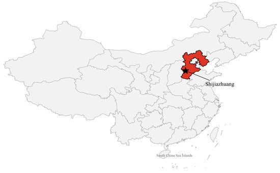
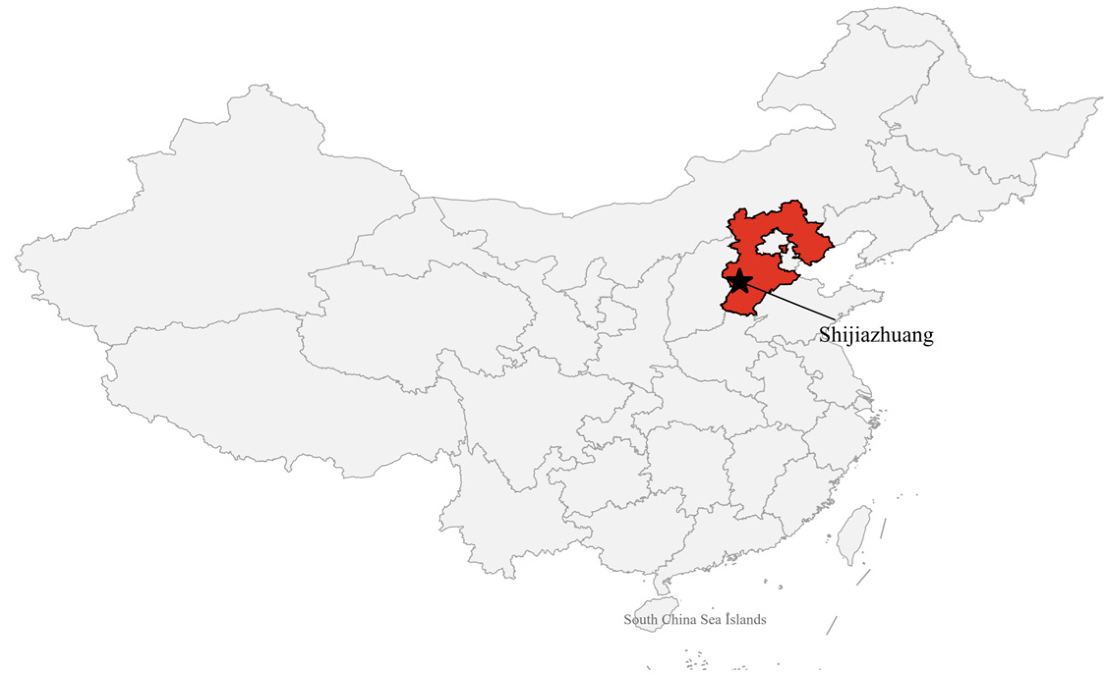
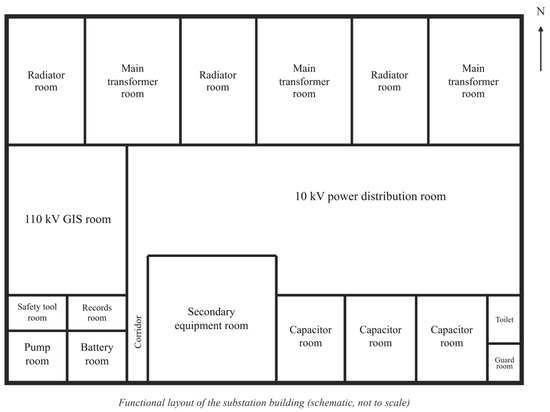
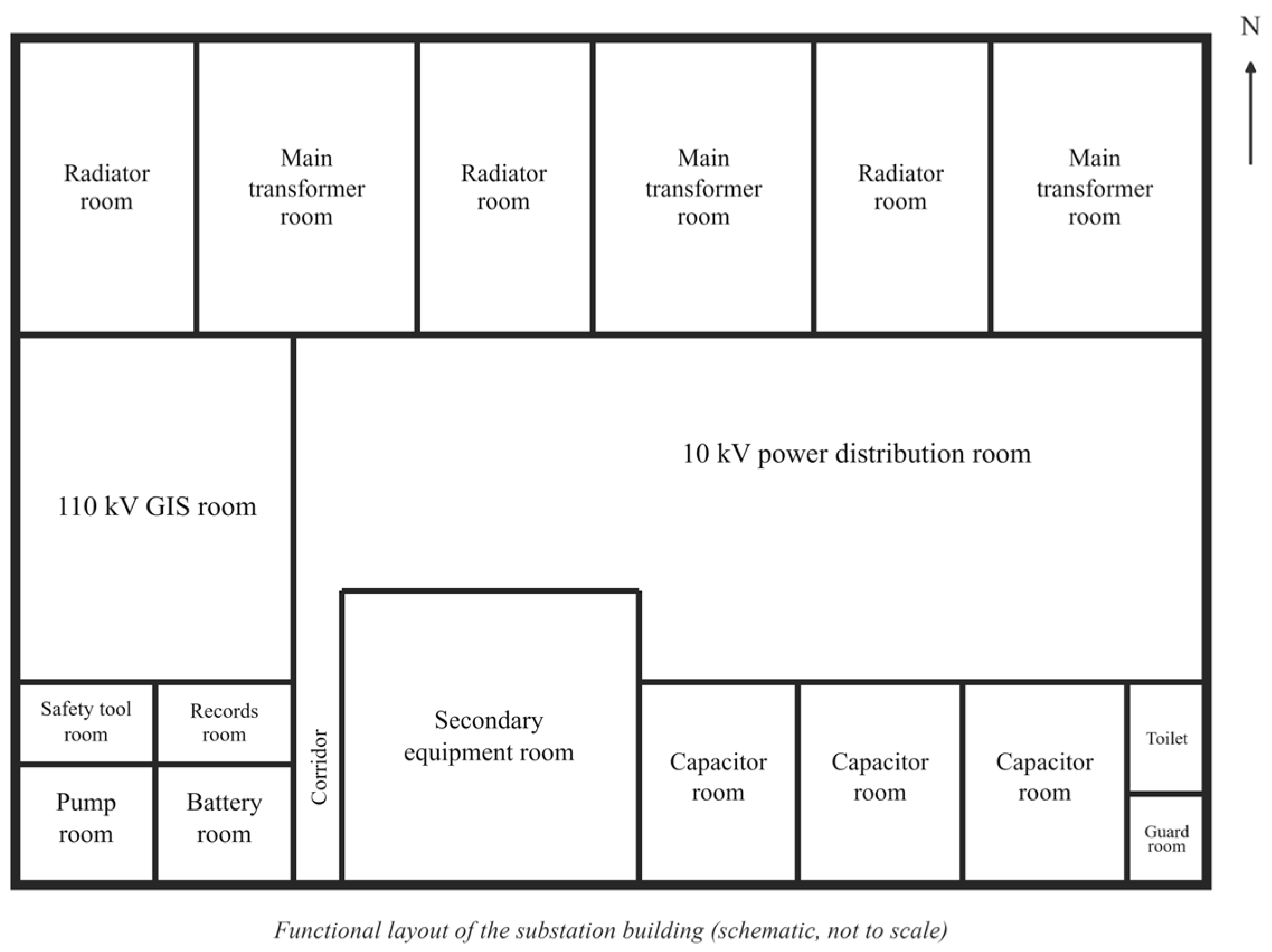
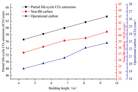
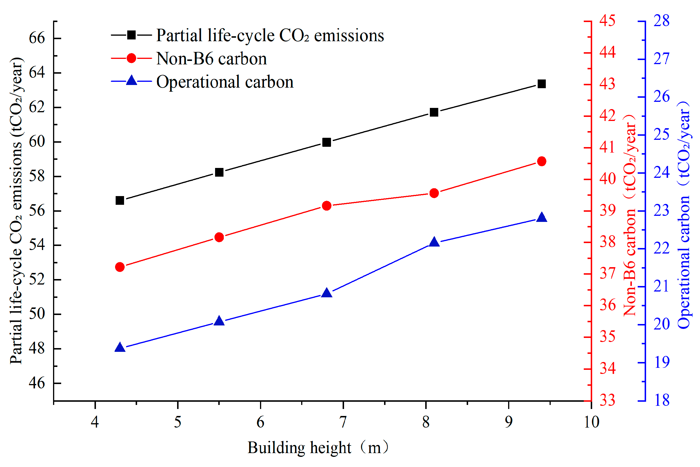
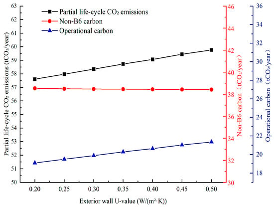
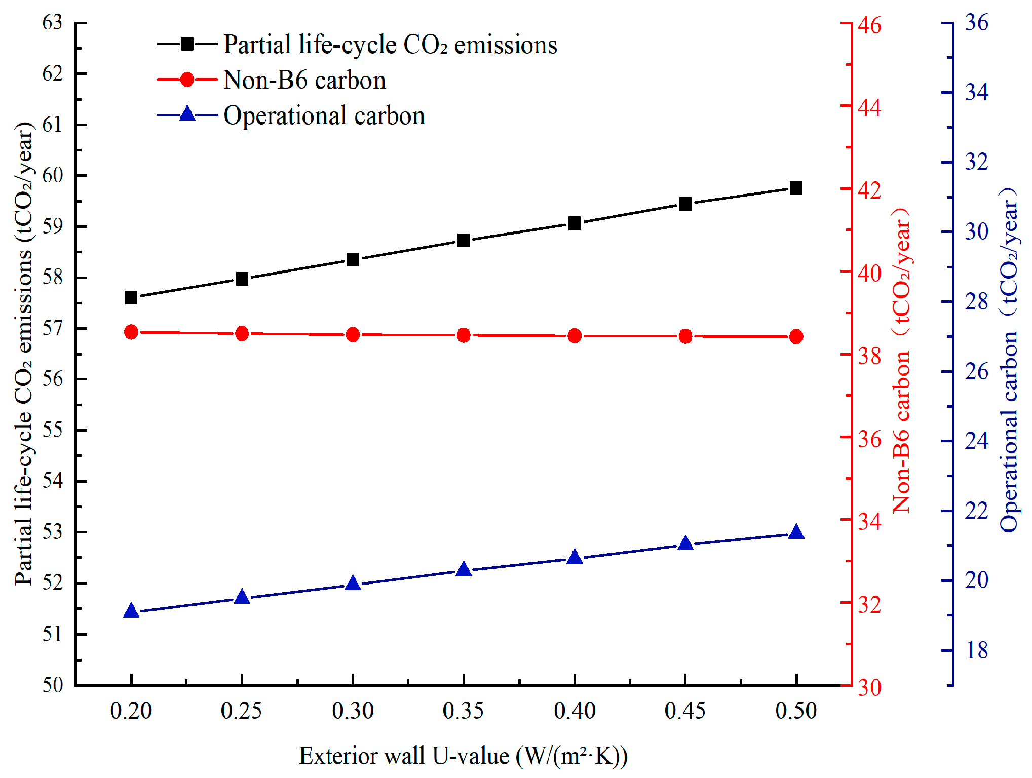
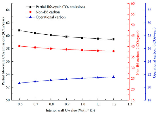
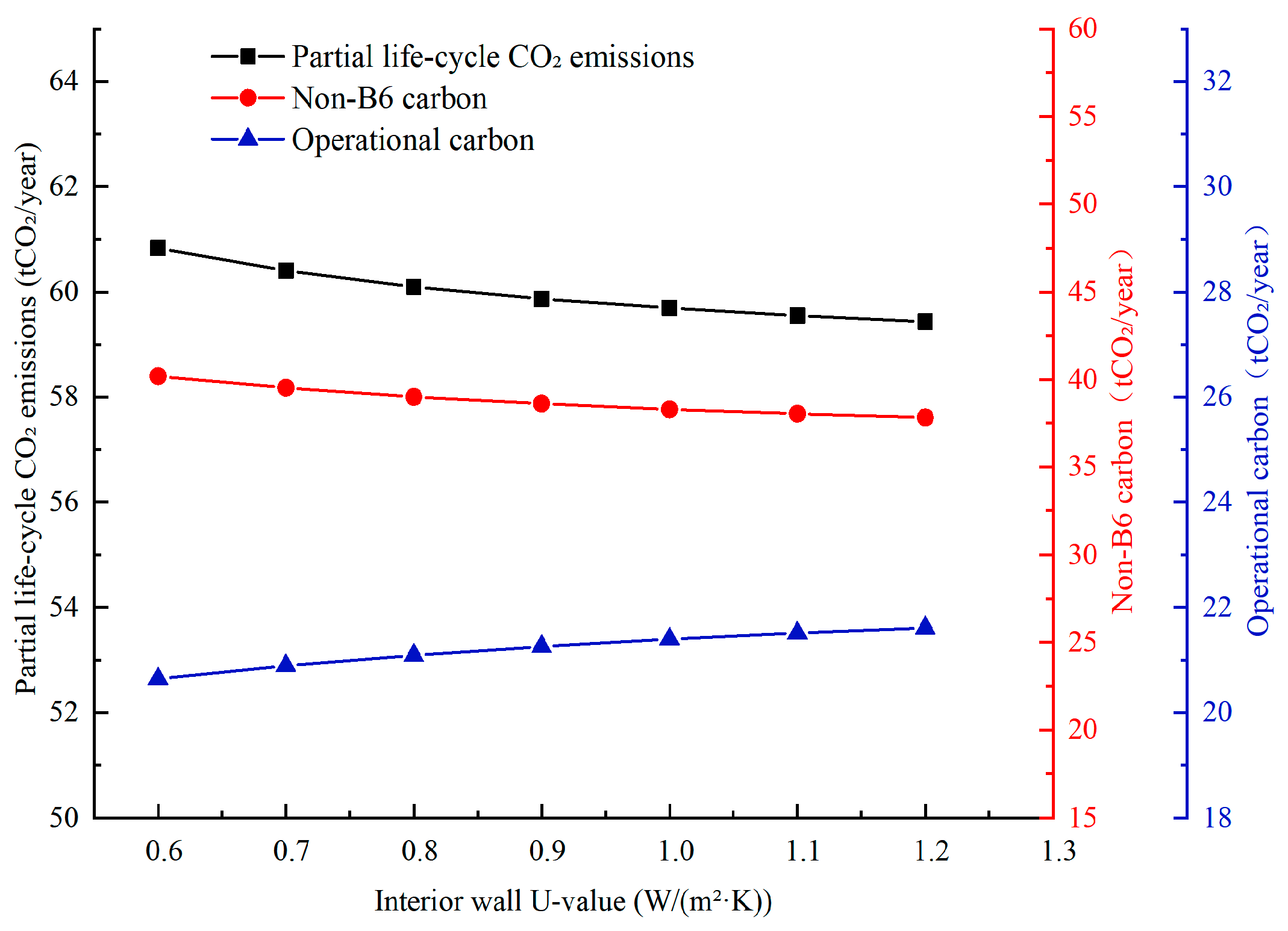
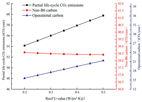
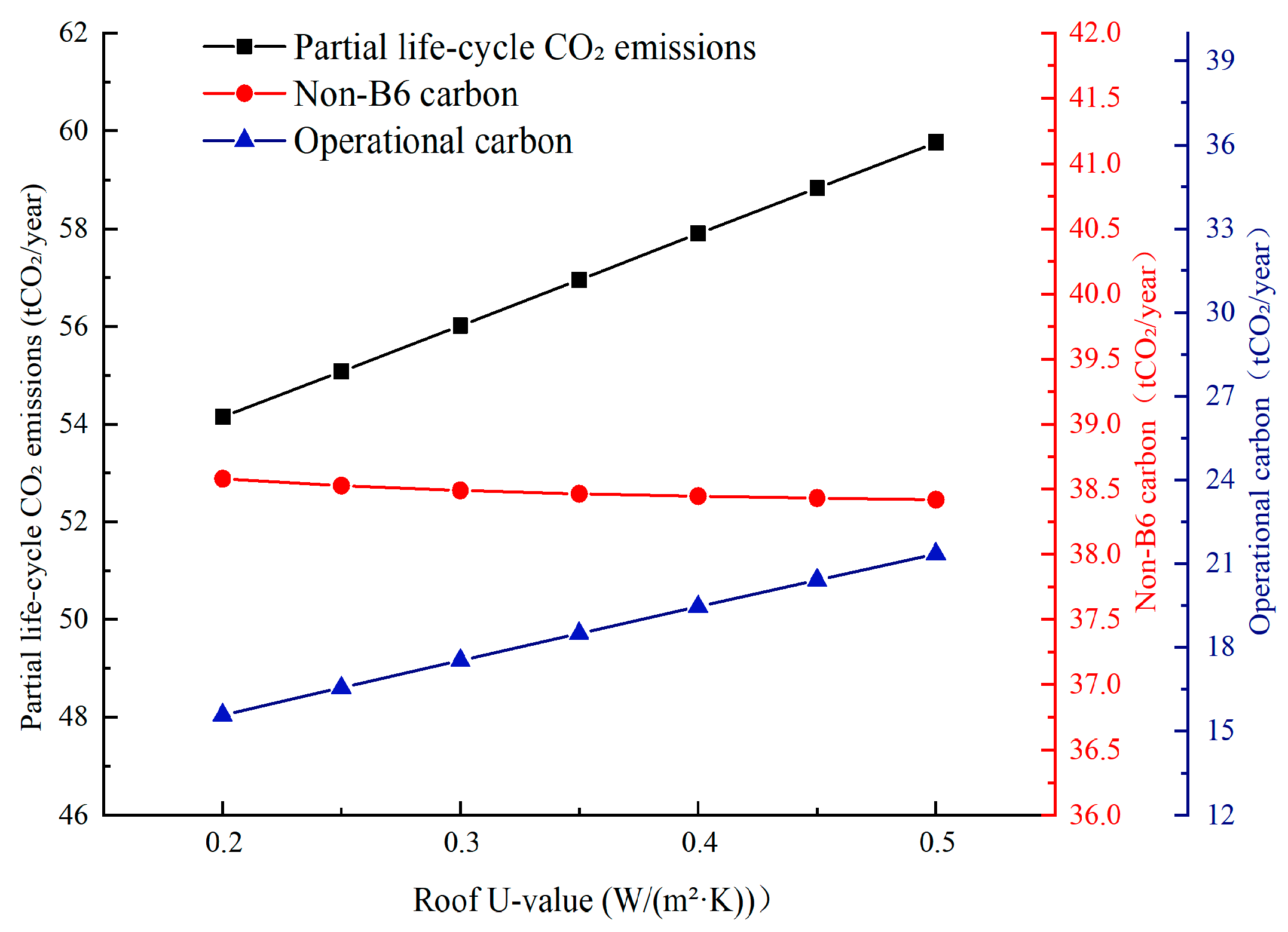
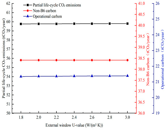
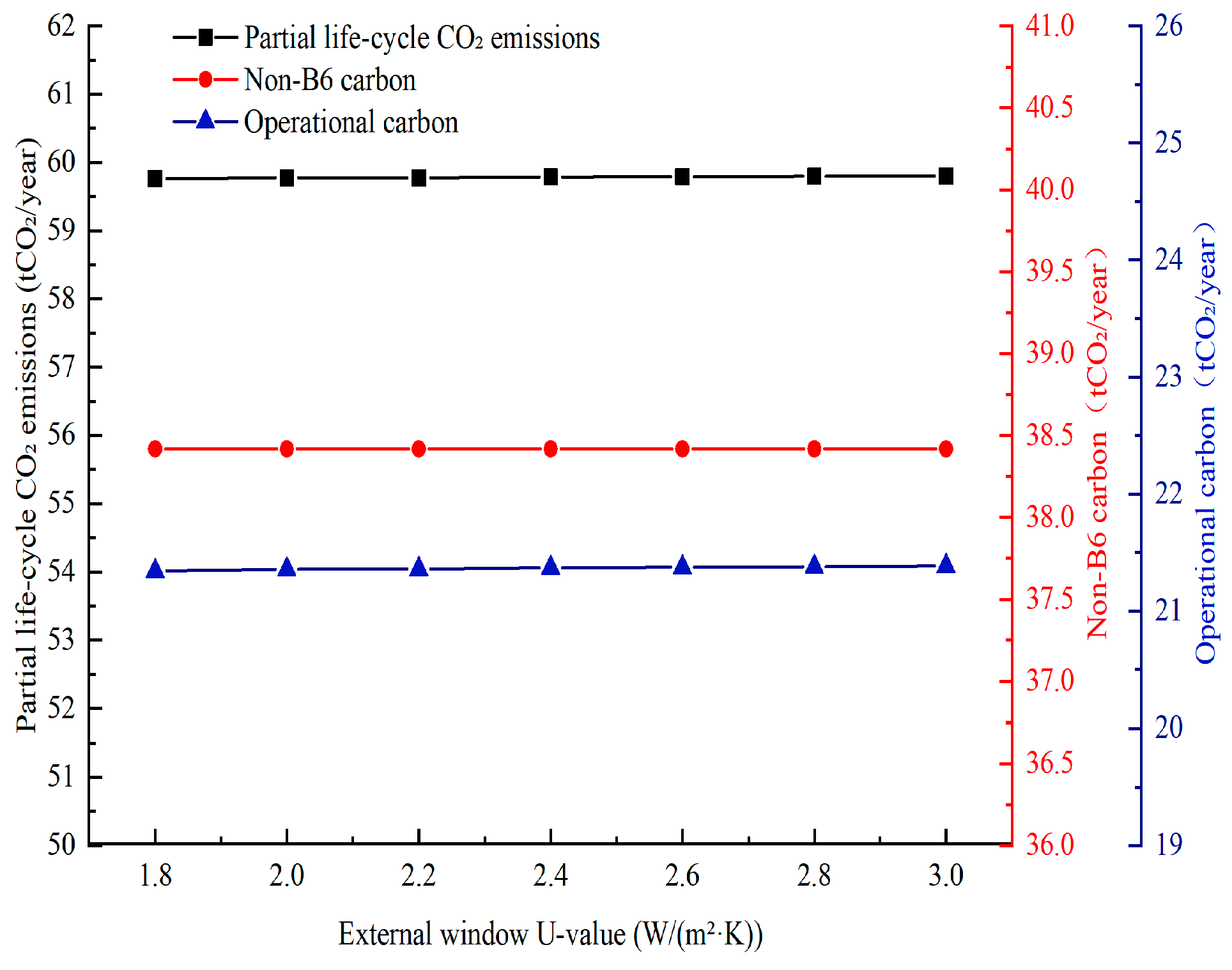
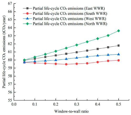
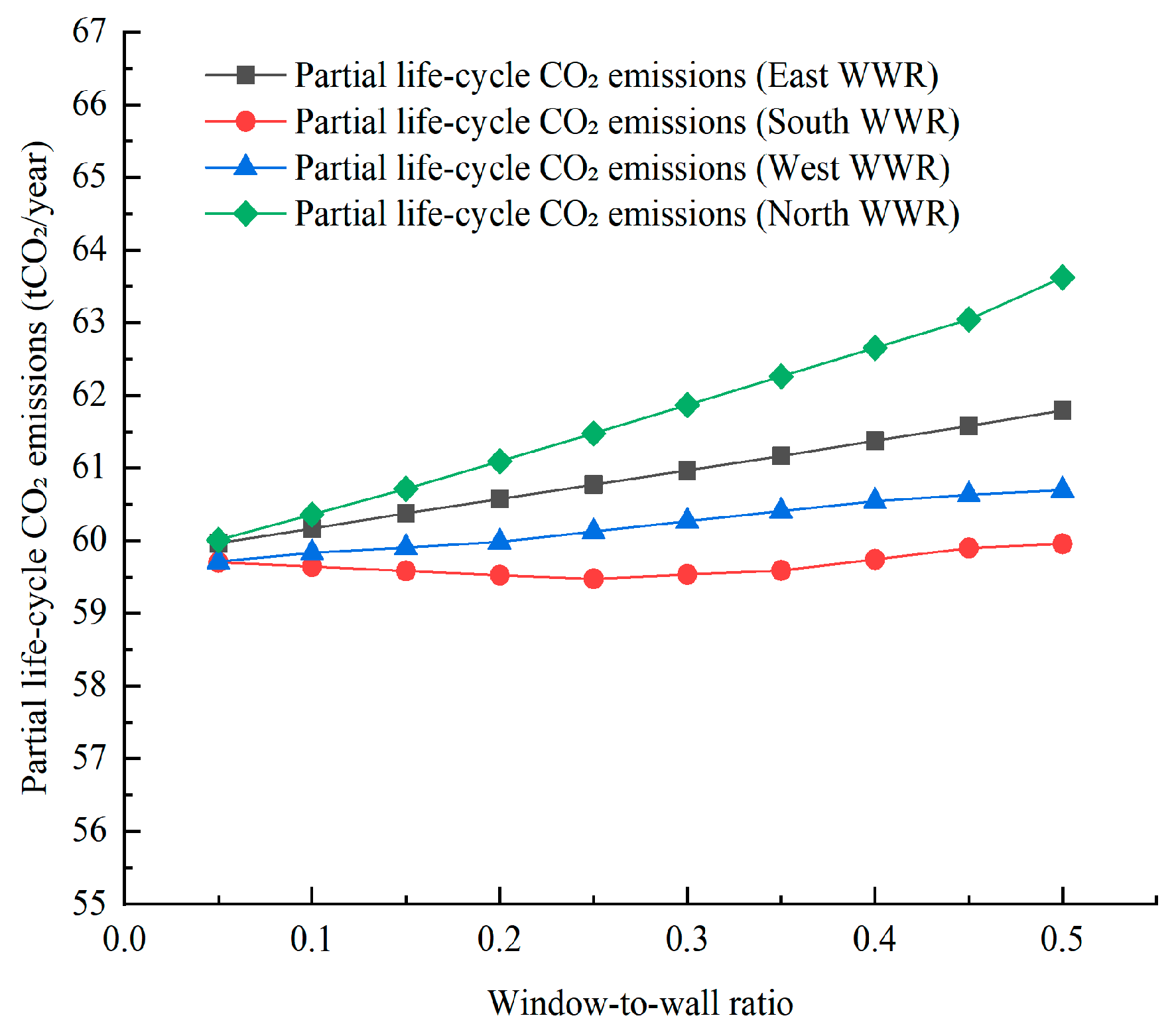
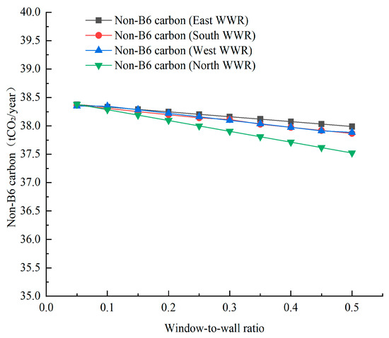
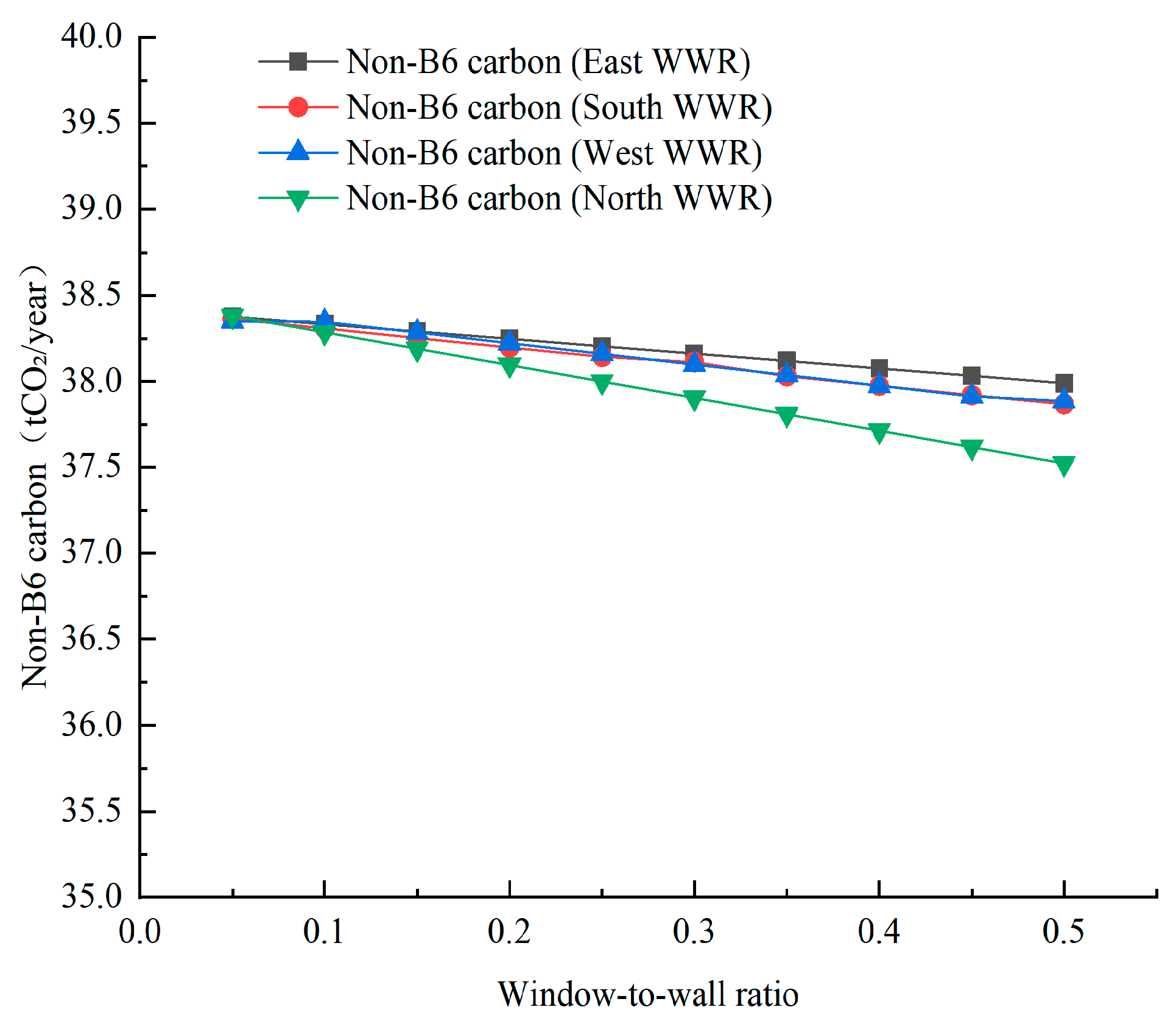
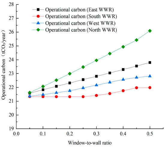
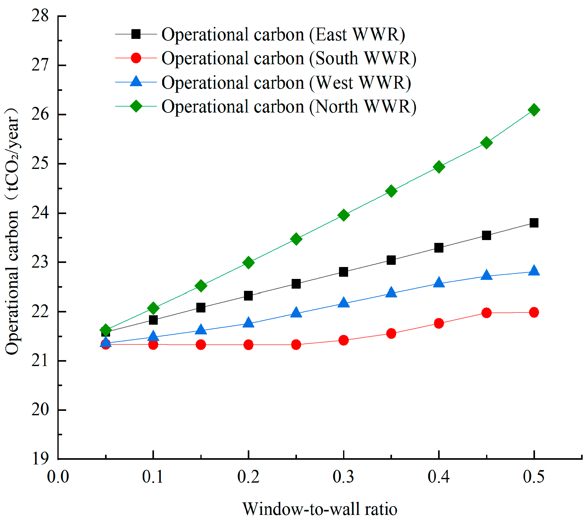
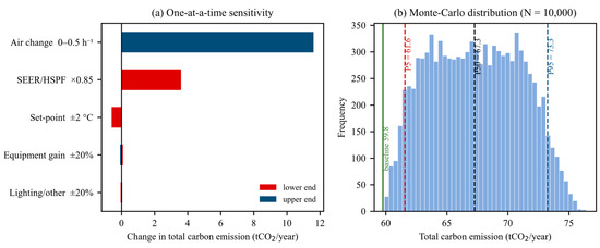
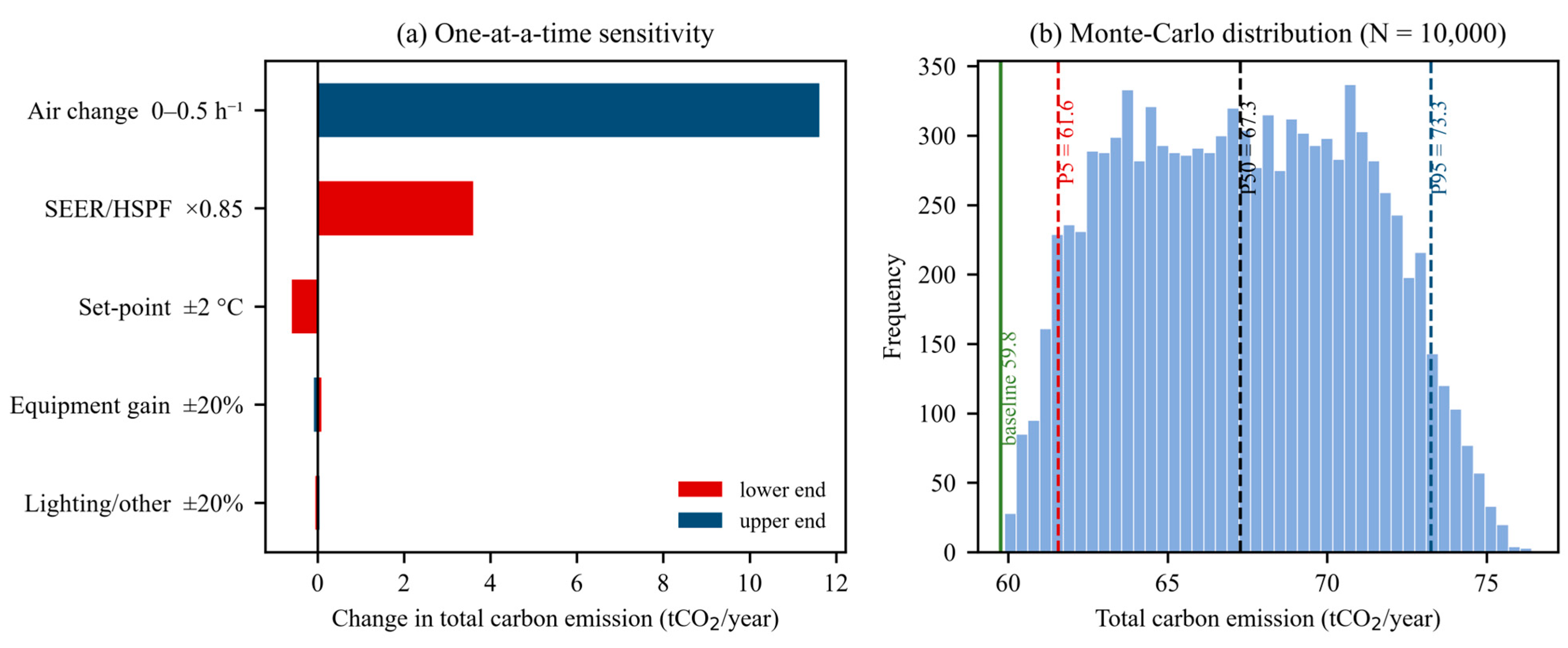

Disclaimer/Publisher’s Note: The statements, opinions and data contained in all publications are solely those of the individual author(s) and contributor(s) and not of MDPI and/or the editor(s). MDPI and/or the editor(s) disclaim responsibility for any injury to people or property resulting from any ideas, methods, instructions or products referred to in the content. |
© 2026 by the authors. Licensee MDPI, Basel, Switzerland. This article is an open access article distributed under the terms and conditions of the Creative Commons Attribution (CC BY) license.