


Abstract
Hospitals are among the most energy-intensive buildings, yet their heating systems often operate below optimal efficiency due to outdated controls and limited sensing. Existing facilities often provide only a few accessible measurement points, many of which are locked within proprietary master controllers and not integrated into the Building Automation System (BAS). To address these limitations, this study proposes a data-driven feature selection approach that supports the development of gray-box emulators for complex, real-world central heating plants. A year of operational and weather data from a large hospital was used to train multiple machine learning models to predict the heating demand and return water temperature of a hospital heating plant system. The model’s performance was evaluated under reduced-sensor conditions by intentionally removing unpredictable values such as the VFD speed and flow rate. XGBoost achieved the highest accuracy with full sensor data and maintained a strong performance when critical sensors were omitted. An explainability analysis using Shapley Additive Explanations (SHAP) is applied to interpret the models, revealing that outdoor temperature and time of day (as an occupancy proxy) are the dominant predictors of boiler load. The results demonstrate that, even under sparse instrumentation, an AI-driven digital twin of the heating plant can reliably capture system dynamics.
1. Introduction
Improving energy efficiency in buildings has become a global priority in the face of climate change and rising energy costs [1]. The building sector accounts for roughly 40% of total energy consumption in developed countries [2], and, among these, hospitals stand out as particularly energy-intensive facilities [3]. Hospitals operate 24/7 and must maintain strict indoor air quality and thermal conditions, resulting in a significantly higher energy use per unit floor area compared to other building types [3]. Indeed, recent analyses indicate that healthcare facilities have the highest energy consumption per square meter of all commercial buildings, contributing on the order of 10% to overall building energy use in some regions [4]. A large portion of this demand comes from heating, ventilation, and air-conditioning (HVAC) systems, which run continuously to support critical hospital functions [5]. Within hospital HVAC systems, boilers are a key component responsible for providing space heating and hot water, making their efficient operation vital for both patient comfort and infection control [6]. Enhancing boiler performance in hospitals, therefore, offers a substantial potential to reduce energy usage and associated carbon emissions while lowering operational costs.
These systems are typically designed with an excess capacity to meet peak load conditions, which means they often operate at a partial load with poor efficiency during normal conditions [7]. In practice, many hospitals (especially older facilities) do not undergo continuous commissioning or regular recalibration of equipment. After the initial installation and occupancy, control setpoints and schedules are frequently left unchanged for years, even as building usage patterns evolve [8]. This lack of ongoing tuning leads to drift and inefficiencies over the building’s life cycle. Overall, legacy infrastructure often provides only limited sensing and uneven data access, while critical parameters are locked inside proprietary controllers and not fully integrated into the BAS, which will yield sparse and sometimes noisy data for analytics. These realities motivate approaches that can extract reliable insight from routine BAS and weather data and guide optimization under real-world constraints.
In recent years, the use of artificial intelligence (AI) and machine learning (ML) techniques in building management has offered promising solutions to improve operational efficiency. Modern BAS platforms can collect large volumes of real-time data, and data-driven analytics can use this data to enable a smarter, adaptive control of complex HVAC systems like hospital boiler plants [9]. Unlike traditional control schemes that rely on fixed schedules or reactive adjustments, ML algorithms can learn the intricate, nonlinear relationships between variables and make predictive decisions to enhance performance. Prior studies have shown that machine learning models can optimize boiler operations by reducing fuel consumption and improving heat delivery, which not only saves energy but also extends equipment life through gentler operation [10]. For example, predictive maintenance applications use ML to analyze sensor trends and detect anomalies, allowing boiler faults or performance degradation to be anticipated and addressed before they lead to failures [11]. Various ML techniques, from neural networks and fuzzy logic controllers to evolutionary optimization algorithms, have been successfully applied to maximize boiler efficiency and minimize emissions [9]. These approaches illustrate the transformative potential of ML models in managing hospital energy systems, where even small efficiency gains can translate to significant cost savings and environmental benefits. At the same time, the diversity of AI methods available underscores the importance of choosing appropriate modeling techniques for a given scenario, as each method has strengths and limitations in capturing the dynamics of boiler behavior. While these studies demonstrate the strong potential of ML in building energy systems, most assume the availability of comprehensive and reliable sensor data, an assumption that often does not hold in existing hospital boiler plants.
In this study, we develop a practical and explainable modeling pipeline for a minimally instrumented hospital heating plant that combines routine BAS and weather data with physics-guided features to predict two operationally important targets: heating demand and return water temperature. The proposed approach is designed for real facilities where key measurements are often unavailable or unreliable; accordingly, we evaluate model robustness through structured reduced-sensor experiments that remove flow and pump VFD signals and quantify the resulting performance impact. Building on this, we use SHAP and selected PDP analyses to interpret the best-performing model and to identify physically meaningful proxy relationships (e.g., when weather and schedule features can substitute for missing plant measurements). The main contribution is a decision-oriented reduced-sensor modeling framework that ties predictive accuracy and interpretability to sensing and metering priorities for under-instrumented heating plants, enabling high-fidelity emulation from routinely accessible data.
In this study, we build a practical, explainable modeling pipeline for a minimally instrumented hospital heating plant that uses BAS and weather data with physics-guided features to predict two critical targets, return water temperature and heating demand, while testing robustness with reduced-sensor inputs. Unlike prior studies that assume complete and reliable instrumentation, this work explicitly addresses the reality of sparse and unreliable sensing in hospital heating plants by deliberately removing key operational measurements such as the flow rate and pump VFD speed. We rank variables by predictive influence and physical plausibility, then run deliberate sensor-removal experiments (e.g., omitting flow or pump speed) to quantify the accuracy penalty and identify when time of day, day type, and weather can stand in as workable proxies. Using comparable regressors trained on identical splits of data, we center interpretation on the best model and pair Shapley Additive Explanations (SHAP) and Partial Dependence Plots (PDP) where appropriate to translate model behavior into clear, engineering-useful insight. The primary and novel contribution of this study is a reduced-sensor, explainability-driven framework that explicitly quantifies how much predictive capability is retained under realistic BAS sensing constraints and converts interpretability results into actionable guidance for sensing priorities, metering decisions, and supervisory-level operational support using only routine BAS data. The resulting models provide a practical emulator of plant behavior suitable for supervisory-level analytics and scenario evaluation, establishing a foundation for scalable digital-twin development and subsequent optimization studies in healthcare facilities.
2. Literature Review
Heating systems in hospitals, typically powered by centralized hot-water or boiler plants, constitute one of the most critical and energy-demanding components of building operations. When these systems are not optimized, their inefficiencies can result in significant energy losses and increased greenhouse gas emissions [12]. Fraile et al. [7] documented a 600-bed hospital’s boiler room and found unstable control causing frequent boiler on/off cycling and wide hot water temperature oscillations. By lowering the minimum firing rate and retuning controller parameters, they succeeded in reducing temperature fluctuations and cycling frequency. Notably, they suggested that more advanced control strategies, such as fuzzy logic, neural network controllers, or predictive control, could further improve boiler responsiveness and efficiency [7]. This example underscores the importance of optimizing hospital heating systems and the need for more sophisticated approaches beyond traditional control loops.
2.1. ML-Based Strategies for Boiler Optimization
In recent years, data-driven machine learning approaches have gained prominence for modeling and forecasting building energy consumption. Traditional physics-based simulations are highly effective for analyzing systems during the design phase; however, they rely on extensive input data and often fail to capture the complexities and irregularities of real-world operational conditions [13]. On the other hand, machine learning models can learn patterns directly from historical data, making them well-suited to capture the complex interactions of weather, occupancy, and controls in operating buildings [14]. Early multi-boiler studies using model predictive control (MPC) demonstrated measurable reductions in fuel use and emissions when heating load forecasting and plant models are coupled with supervisory control logic [10]. Their MPC system achieved measurable reductions in greenhouse gas emissions (approximately 1.3–2.8% CO2 reductions over a few months). While the percentage gains were modest, the results were statistically significant, translating to 45–77 tons of CO2 avoided, and demonstrated the principle that smarter control logic can yield tangible efficiency improvements in real facilities [10]. In more controlled experiments, even larger savings have been reported. For instance, Stock et al. (2021) coupled data-driven models with an optimization algorithm in a high-rise building’s HVAC system, and simulation results indicated up to 70% heating energy savings compared to a conventional setpoint strategy, all without any physical equipment changes [8]. Notably, these approaches are low-cost and rapidly deployable, since they rely only on software and analytics applied to existing Building Automation System (BAS) data [8]. Beyond model predictive control, intelligent optimization algorithms have been explored for boiler combustion and efficiency tuning. Liang et al. [1] survey the landscape of boiler combustion optimization and note that evolutionary algorithms like genetic algorithms (GAs) have gained significant attention as a means to improve energy efficiency and reduce emissions [1]. Indeed, evolutionary meta-heuristic algorithms (e.g., GA-type approaches) can automatically search for optimal boiler setpoints and configurations in complex nonlinear systems which are impractical to tune manually. A range of machine learning methods, including expert systems, fuzzy logic control, support vector machines (SVMs), artificial neural networks (ANNs), and hybrid models combining multiple approaches, have been applied to energy consumption optimization [15]. These methods have shown the ability to improve combustion efficiency and minimize pollutants by continuously learning and adjusting to operating data [9]. For example, Nemitallah et al. [9] review dozens of such applications and conclude that AI-based techniques are “great tools towards better performance of boilers at minimum emissions,” provided they are implemented with proper data and model selection [9]. The same review emphasizes that machine learning methods (including ANN, GA, SVM, and others) can effectively handle the complex trade-off between boiler efficiency and NOx emissions [9,16]. Overall, these studies reflect a growing confidence in the capacity of computational intelligence to enhance, and in some instances even outperform, traditional boiler control methods.
In particular, advanced learning algorithms are becoming more common in building energy systems. Gradient-boosting ensemble models (e.g., XGBoost) have been proposed for boiler performance modeling, often combined with hyperparameter tuning techniques like Bayesian optimization to boost predictive accuracy [17]. Likewise, researchers have explored advanced machine learning techniques such as gene expression programming (GEP) and Group Method of Data Handling (GMDH) networks for building energy forecasting, achieving a high prediction accuracy for short-term energy use [18]. In their study, GMDH slightly outperformed GEP in accuracy, though at the cost of greater model complexity [18]. Deep neural networks are also being deployed within control frameworks; for instance, recurrent neural networks (LSTMs) have been integrated into hybrid MPC schemes to predict indoor temperatures and were optimized via algorithms like particle swarm optimization for HVAC control [10]. These data-driven approaches often use cloud computing, IoT connectivity, and digital-twin frameworks to continuously mirror and learn from live building operations [8]. As computing power and data availability have increased, it has become feasible to replace detailed physics-based HVAC models with trained black-box models that can be quickly scaled across many buildings [8]. Researchers note that, while traditional white-box models (e.g., building energy simulations) offer accuracy, developing a bespoke model for each building is labor-intensive and requires expert calibration [8]. Data-driven models address this limitation by learning directly from real operational data, making them particularly appealing for quick implementation in existing buildings where developing detailed simulations is often constrained by time or limited expertise.
2.2. Feature Selection and Data-Driven Modeling
Alongside the development of control algorithms, scholars emphasize the critical role of feature selection, which is identifying which input variables or sensor measurements are most informative in creating effective data-driven models for boiler optimization [19]. In building energy modeling, typical features include outdoor weather conditions, temporal indicators (hour of day, day of week, season), occupancy-related metrics, and operational parameters of HVAC systems [20].
Nikula et al. [21] introduced a data-driven framework for monitoring steam boiler performance that illustrates this point well. Their framework uses an information-theoretic variable ranking method to determine which process variables have the strongest correlation with boiler efficiency [21]. By analyzing historical operating data from two large industrial boilers, they consistently found a subset of variables that governed efficiency (despite the two boilers being of different designs). In practice, the approach monitors the boiler’s real-time efficiency against an expected optimal efficiency (learned from historical best-performance data) and uses the top-ranked variables, including proxy-sensed indicators where direct measurements are unavailable, to define the process state [21]. Significant deviations between the current efficiency and the historical benchmark signal potential faults or suboptimal operation. This study demonstrated that focusing on key features (identified via variable importance metrics) enables real-time performance tracking and the early detection of efficiency drops [21].
In the case of hospitals, occupancy and scheduling information can be especially significant—for example, patterns of patient admissions, staff working hours, or operating room usage can create distinctive energy demand signatures [15]. A comprehensive review by Amasyali and El-Gohary [22] cataloged the typical features employed across dozens of data-driven building studies, finding that weather parameters, occupancy patterns, and operational schedules were among the most frequently utilized inputs. In many hospital-focused studies, occupancy and meteorological data have indeed emerged as key predictors of energy use [15]. Empirical studies have shown that variables such as patient counts, staff schedules, and daily hospital activities shape distinctive load profiles [23,24]. However, a noted shortcoming is that not all works deeply analyze why those features matter or how sensitive the models are to them [15]. For instance, some papers include variables like occupancy or indoor air temperature without discussing the temporal dynamics or the building’s operational context behind those numbers [15].
Another important consideration is data preprocessing and feature engineering. Raw hospital energy data often contain noise, missing values, and outliers arising from sensor faults, as well as mixed temporal resolutions. Techniques such as data cleaning, normalization, temporal aggregation, and the creation of new features (e.g., degree-day indicators or occupancy density metrics) are commonly applied, and studies have reported significant performance improvements when such preprocessing is conducted [23,24,25]. One systematic review emphasized that advanced data preprocessing and feature engineering were crucial for improving model performance in building energy forecasts [15]. For instance, the smoothing or filtering of time series inputs has been shown to help neural network models capture underlying trends more effectively [23], while lagged features such as the previous hour’s energy consumption substantially enhance short-term prediction accuracy [24]. Similarly, studies employing dimensionality reduction via PCA [26] or a clustering of similar operational days [22] have reported notable gains in forecast robustness. The diversity of data preparation strategies means that results can sometimes be hard to compare across studies. Thus, recent authors have called for a more transparent and standardized reporting of preprocessing steps [15]. Therefore, choosing the right inputs and handling data wisely is just as important as the choice of the ML model itself. Effective feature selection (including domain-specific knowledge about what drives energy use in a hospital) and rigorous preprocessing are repeatedly cited as the best practices for achieving high accuracy. These efforts also help ensure that the model’s predictions are based on meaningful signals rather than artifacts or noise.
2.3. Model Interpretability and Research Gaps
One theme that has become increasingly important is the interpretability of AI models in the energy domain. As models grow more sophisticated, such as deep neural networks, ensemble hybrids, etc., they often behave as black boxes, producing predictions without a clear relationship between inputs and outputs [27]. In the context of building operations—especially critical facilities such as hospitals—this lack of transparency can be problematic [27]. Facility managers and engineers are more likely to trust and adopt an AI system if they can understand the basis for its recommendations. Recognizing this, researchers have started to apply explainable AI (XAI) techniques to building energy models [28]. One prominent example is the use of SHAP values, a method based on cooperative game theory that attributes the output of a model to its input features [28]. By applying SHAP to a trained energy model, one can determine, for instance, how much of a hospital’s energy use prediction is driven by outdoor temperature versus occupancy on a particular day [29]. This has proven insightful in case studies; for example, Henkel et al. [29] combined SHAP with a data-driven MPC controller to interpret the controller’s learned model, finding that SHAP analysis could reveal feature effects and model weaknesses that were not obvious upfront. Such interpretability tools help identify whether the AI is making decisions for sensible reasons or for spurious correlations [30].
With respect to model explainability, SHAP is an algorithm introduced to the machine learning community by Lundberg and Lee [31]. SHAP estimates how much each feature contributes to a model’s prediction by evaluating all possible combinations of features and distributing the difference between the actual prediction and the average output in a mathematically fair manner. A positive SHAP value indicates that a feature increases the predicted value relative to the dataset’s average, while a negative value indicates that it decreases it. Summing the SHAP values across all features reproduces the exact model prediction for that instance, an additive property that makes SHAP uniquely consistent and locally accurate for attribution. While SHAP provides instance-level explanations, PDPs complement this by offering a global view of how individual features influence the model’s predictions. PDPs show the expected model output as a function of one feature while holding all other variables constant, making them useful for visualizing broad trends and confirming whether the learned relationships align with domain knowledge [27].
In summary, the cited studies demonstrate a wide range of AI techniques (from MPC and ANN controllers to genetic algorithms and ensemble models) that have successfully improved boiler and HVAC performance. They show that data-driven methods can yield meaningful efficiency and emission gains in simulations or controlled experiments. However, these studies also reveal common limitations: most assume relatively complete sensor data and do not test models under the sparse, noisy conditions typical of hospital plants. In hospital-specific research, occupancy and weather are consistently identified as important features, yet few works quantify how dependent their models are on these inputs or how performance degrades when key sensors are unavailable. This highlights a research gap in understanding how data-driven methods perform under sparse sensors and how their predictions can be made interpretable for critical facilities like hospitals. Our work addresses these gaps by focusing on a minimally instrumented real hospital heating plant and integrating an explainable AI approach using SHAP to identify key drivers of boiler performance. By using domain knowledge to select and engineer features from the BAS and weather data, and by comparing different machine learning algorithms, we identify the critical drivers of boiler efficiency. Crucially, we systematically evaluate model robustness by deliberately removing flow and VFD speed sensors to check if time-based proxies (hour of day, day type) can sustain accuracy when some real-time measurements are missing. This work therefore extends the literature by demonstrating how a feature-driven, hybrid modeling approach can work reliably in an under-instrumented hospital setting.
3. Materials and Methods
Our study follows a step-by-step process that includes data preparation, feature selection, model development, and interpretability analysis. We start by cleaning and improving the raw data; then, we identify the most useful features, build predictive models, and finally use explainability methods to understand how the model behaves.
3.1. Data Source and Preprocessing
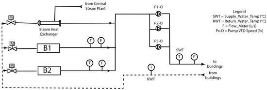
The case study hospital in British Columbia granted us access to its BAS, allowing for the use of real-time and trended operational data for model development. The facility is served by a central plant that provides chilled water, heating hot water, and process steam. Heating hot water is generated by two condensing boilers and a backup heat exchanger providing heat from the steam generation plant, operating on a variable-flow primary loop (Figure 1). The heating hot-water plant is equipped with two identical fire-tube boilers (Vitomax 200-LW, Viessmann Manufacturing Company Inc., Waterloo, ON, Canada), each with a nominal thermal output of approximately 3.0 MW, operated under a variable-flow primary loop configuration. This primary loop is driven by a triplex pump system manufactured by Grundfos (Grundfos Canada Inc., Oakville, ON, Canada), and connects to several secondary loops that distribute heat across the hospital buildings. The full BAS shop drawings were reviewed to understand the heating system’s control logic, which informed the feature selection process described later. Discussions with the control contractor indicated that some measured points were unreliable, most notably the individual boiler flow meters, because site constraints prevented installations in ideal locations, making them unreliable even for relative readings. Acknowledging this, it was confirmed that the master boiler controller commands an equal boiler flow during high-heating-demand periods when both units are active, allowing for an equal split assumption for boiler-level allocation when needed. The flow rate used in Equation (1) is the plant main loop flow measurement (not the individual boiler meters); therefore, uncertainty in boiler-level flow meters does not directly propagate into the heating demand target.
Figure 1.
Simplified version of BAS heating hot water system control schematic.
Data include a full year of timestamped operational data and external weather observations. The raw data were originally recorded at 10 min intervals and were cleaned and standardized before being resampled to an hourly average time step to ensure a uniform temporal spacing and reduce measurement noise. Prior to resampling, all variables were explicitly screened for missing values at the native 10 min resolution. Only a very small fraction of missing data was identified, with a maximum of approximately 1.4% for a limited number of plant variables, while most variables exhibited zero missingness. These missing values occurred as short, isolated gaps consistent with transient sensor dropouts. Forward fill was applied only at the 10 min resolution to bridge these short gaps and preserve temporal continuity, after which hourly averages were computed from the gap-handled data. Given the low missing fraction, the short duration of gaps, and the subsequent hourly aggregation, this preprocessing step is not expected to introduce artificial persistence or inflate model accuracy. In addition, outlier detection was performed by flagging values beyond interquartile range (IQR) thresholds or exhibiting abnormal spikes, and any readings exceeding physical constraints (e.g., negative flow rates or implausible temperature values) were corrected or removed to ensure data quality.
3.2. Data Engineering
The heating plant of the hospital uses three primary pumps with Variable Frequency Drive speeds (VFDs) operating in an alternating pattern (one pump on standby while two are active). We combined the VFD speeds of these three pumps into a single total VFD speed feature used as a proxy for total flow. We also computed an average supply water temperature across the boilers to use when more than one boiler is running, ensuring a representative supply temperature feature even if multiple boilers contribute heat. Given that the two boilers are of the same capacity with the same controls, their supply temperatures should be consistent, making this a reasonable simplification.
We introduce a categorical day type feature to represent the hospital’s operational schedule. Each timestamp was labeled as a weekday, weekend, or holiday, and further segmented by hour of the day. This helps to capture occupancy-related patterns, since hospitals exhibit different load profiles on weekends/holidays versus weekdays. Incorporating day type and hour as features allows the model to infer occupancy trends, which are important for explaining energy demand variations. We one-hot encoded the day type categories so that machine learning algorithms can utilize these as binary features. Beyond the outdoor air temperature, the other weather features used were pressure, humidity, wind speed, and notably wind direction, which was decomposed into sine and cosine components to encode this cyclical variable in a model-friendly numeric form. Short-term historical dynamics were captured through temporal features derived from the outdoor air temperature (OAT), which is a major driver of heating demand. Specifically, we introduced three lagged variables representing the OAT at one-, two-, and three-hour intervals before the current timestamp, as well as a rolling mean over the previous three hours. These engineered features allow the models to recognize gradual changes in weather conditions and capture the system’s thermal inertia, such as the delayed response of heating demand or return water temperature to outdoor temperature fluctuations.
The dataset did not directly record how much heat the boilers supplied, so we estimated the thermal power output, which we then treated as the building’s heating demand. This was calculated using the standard heat transfer Equation (1), based on the measured water flow rate and the temperature difference between the supply and return water.
where is the mass flow rate of water, is the specific heat capacity of water, and is the temperature difference between the supply and return water. By using consistent units (with water density and heat capacity appropriate for the temperature range), this yielded the heating demand in kW for each timestamp. Finally, to harmonize features measured on different scales, all input variables were normalized to a 0 to 1 range via Min-Max scaling. This normalization ensured that variables (e.g., temperatures, flow rates, percentages) were dimensionless and comparable in the modeling algorithms. Table 1 summarizes the features used in this study, along with their respective roles in the analysis.
Table 1.
Description of engineered and operational features used in model development.
3.3. Feature Scenarios
To study how much the actuation-related inputs matter, we defined two different feature set scenarios. In the “Full” scenario, the model used all available inputs, including sensor readings, control signals such as pump VFD speeds and flow rates, and weather data. In the “Reduced” scenario, certain variables such as the water flow rate and pump VFD speed features were omitted, as these are load-dependent and cannot be directly forecast. Since these variables are strong direct indicators of boiler operation, the reduced scenario simulates a case where the model must rely on more indirect predictors (like time of day, temperatures, and weather) to infer the heating output. By comparing these scenarios, we can analyze how much predictive accuracy drops when key data are unavailable, thereby evaluating how well other features (e.g., outdoor conditions or occupancy schedule) can serve as proxies for them. In addition to the full and reduced-sensor configurations, a structured weather feature ablation was conducted using the best-performing model identified in the mentioned scenario comparison to quantify whether secondary meteorological variables materially improve model performance or primarily act as noise. Starting from a baseline feature set consisting of outdoor air temperature (including lagged and rolling features) and time-based variables (hour of day and day type), weather inputs were incrementally added in the following order: relative humidity, barometric pressure, wind speed, and wind direction. This progressive inclusion strategy enables the direct attribution of performance changes to individual weather variables while holding the core thermal and schedule-related drivers constant. In all reduced-sensor experiments, only non-forecastable operational signals (flow rate and pump VFD speed) were removed; supply water temperature was retained, as it is routinely available from the BAS and represents a supervisory-level state variable rather than a directly controlled actuation signal.
3.4. Predicted Variables
In this study, we focused on predicting two key output variables that characterize the central heating plant’s performance. The first one is the heating demand (kW), the thermal power output being delivered by the boilers to the building at each hour. This is calculated as described above and represents the instantaneous heating load on the system. The second one is the return water temperature (°C), which is the temperature of water returning to the boilers from the heating loop. The return temperature is an important indicator of the boiler state (condensing vs. non-condensing mode) and efficiency (a lower return temperature generally implies more heat was extracted in the loop). Separate predictive models were developed for each target. Both target variables are continuous and were normalized during modeling, though all error metrics (see below) are reported in a normalized form for interpretability.
3.5. Modeling Approach
For each target variable and feature scenario, we trained supervised learning models to learn the relationship between the input features and the outputs. A diverse set of regression algorithms were implemented to determine which modeling approach best captures the system behavior. Multiple machine learning models were evaluated to provide a comparative benchmark across linear, nonlinear, and ensemble-based approaches commonly used in building energy modeling. This comparative evaluation was intended to assess predictive performance, robustness, and interpretability rather than to exhaustively tune every possible algorithmic variant.
- Linear Models: We used two regularized linear regressors: Lasso and Ridge regression. These models are simple to implement and fast and also offer interpretable coefficients [32]. Ridge (L2-regularized) was evaluated alongside Lasso to see whether a slightly different regularization would improve performance for variables that may be collinear.
- Ensemble Tree-Based Models: We tested Random Forest and gradient boosting methods (including XGBoost). These ensemble algorithms can model complex nonlinear behavior and often yield a high accuracy for structured data [33]. Random Forest, as noted, also gives insight into feature importance by design [34]. Gradient boosting builds trees sequentially and often achieves a better accuracy through boosting, at the risk of more hyperparameters to tune [33]. Both types of ensembles were considered to use their ability to capture the heating system’s nonlinear response.
- Support Vector Regression (SVR): We evaluated an SVR model with a nonlinear kernel to see if a kernel-based method could find the relationships with fewer parameters. SVR can model nonlinear functions in a feature space with a lot of dimensions, and it is resistant to overfitting if the kernel and regularization are chosen well.
All machine learning models were implemented in Python (v3.10.9) using the scikit-learn (v1.2.1) and XGBoost (v3.0.1) libraries; we kept all hyperparameters mostly at default values (or minimally tuned) to ensure a fair comparison among different models. The modeling process then focused on comparing how effectively the different algorithms captured the behavior of the hospital heating plant data and how their performance changed when key sensors were eliminated. Different Python libraries have been used, including Pandas for data preparation, scikit-learn for modeling, and Matplotlib (v3.7.0) for visualization.
3.6. Explainability Methods (SHAP and PDP)
To interpret model behavior, we computed SHAP values, which attribute each prediction to input features using a game-theoretic decomposition. We computed SHAP primarily on the best-performing tree ensemble (XGBoost) because it consistently delivered the highest accuracy for both targets and both sensor scenarios; this ensured that the explanations reflected our strongest model.
We also generated Partial Dependence Plots (PDPs) to visualize the average marginal effect of selected features (hour of day) on the predicted target. By plotting this relationship, one can observe how changes in that feature alone drive the predicted output. This allows us to determine if the model has learned a meaningful relationship between the feature and the target. We focused on the hour of day because daily operational routines are the main drivers of heating load and become especially important when direct plant sensors (flow/VFD) are unavailable. Accordingly, the PDPs were computed for the reduced-sensor XGBoost models, letting us isolate how time of day alone shapes the predicted heating demand and return water temperature and to confirm the schedule-driven patterns observed in our results.
4. Results
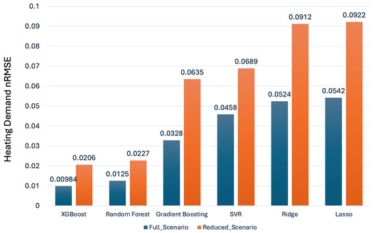
Models were evaluated using standard performance metrics, including the normalized Mean Absolute Error (nMAE), normalized Root Mean Squared Error (nRMSE), and the coefficient of determination (R2), to assess the predictions of both heating demand and return water temperature under full and reduced-input scenarios (Table 2, Table 3, Table 4, Table 5, Table 6 and Table 7). Both target variables were Min–Max normalized to the [0, 1] range prior to modeling; accordingly, nRMSE and nMAE are unitless and represent the relative prediction error with respect to each target’s operating range. Over the analyzed year, the heating demand varied between approximately 960 and 4300 kW, while the return water temperature ranged between 56 and 64 °C. Across both targets, the models achieved low error values, with XGBoost and Random Forest consistently outperforming the other algorithms. For heating demand, XGBoost produced the lowest errors in the full-input scenario (nRMSE = 0.010, nMAE = 0.007), indicating that the model accurately captured load dynamics. Even when the feature set was reduced, the error levels remained small (nRMSE = 0.021, nMAE = 0.015), demonstrating a robust inference capability under reduced-sensor conditions. Random Forest followed a similar pattern, with only slightly higher errors.
Table 2.
Comparison of performance metrics for heating demand prediction across different model configurations (nRMSE).
Table 3.
Comparison of performance metrics for heating demand prediction across different model configurations (nMAE).
Table 4.
Comparison of performance metrics for heating demand prediction across different model configurations, .
Table 5.
Comparison of performance metrics for return water temperature prediction across different model configurations (nRMSE).
Table 6.
Comparison of performance metrics for return water temperature prediction across different model configurations (nMAE).
Table 7.
Comparison of performance metrics for return water temperature prediction across different model configurations, .
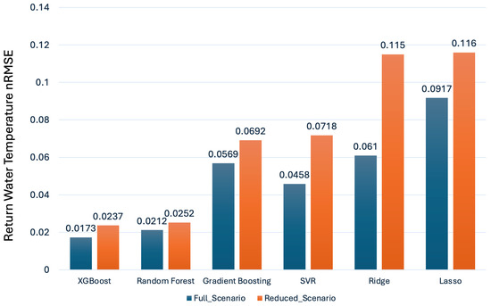
The return water temperature results mirrored these trends. XGBoost again achieved the strongest performance, yielding an nRMSE of 0.017 in the full-input case. Under the reduced-sensor setup, the increase in error was modest (nRMSE = 0.024), indicating a stable performance even without direct flow and VFD signals. Although R2 values remained high, the consistently low nRMSE and nMAE across both targets and scenarios indicate that the ensemble models effectively captured system dynamics and maintained robustness under reduced-sensor conditions. The XGBoost model was configured with 600 trees, a maximum depth of 6, a learning rate of 0.05, and row and feature subsampling ratios of 0.8. These hyperparameters were selected to balance model expressiveness and regularization in building energy forecasting.
On the other hand, the simpler algorithms, such as Lasso, Ridge, and Support Vector Regression, showed a noticeably weaker performance (Figure 2 and Figure 3). Their R2 values were generally lower and their errors higher, especially in the reduced-input case. This gap is likely due to their limited ability to capture nonlinear dependencies and feature interactions that dominate the heating system’s behavior. While linear models can approximate general trends, they struggle with complex cross-effects among temperature, pressure, and time-related variables. SVR performed somewhat better than the purely linear regressors but was still sensitive to kernel and scaling choices, making it less stable under changing input conditions. These comparisons highlight why ensemble tree-based methods like XGBoost and Random Forest outperform others for this application. They can model nonlinear relationships, automatically handle variable interactions, and remain robust when some sensor inputs are unavailable. The results demonstrate that, although all models learned the general direction of the heating and temperature trends, only the ensemble approaches achieved the accuracy and stability required for reliable operational prediction in real-world hospital settings.
Figure 2.
Comparison of nRMSE values across all models in both scenarios (return water temperature).
Figure 3.
Comparison of nRMSE values across all models in both scenarios (heating demand).
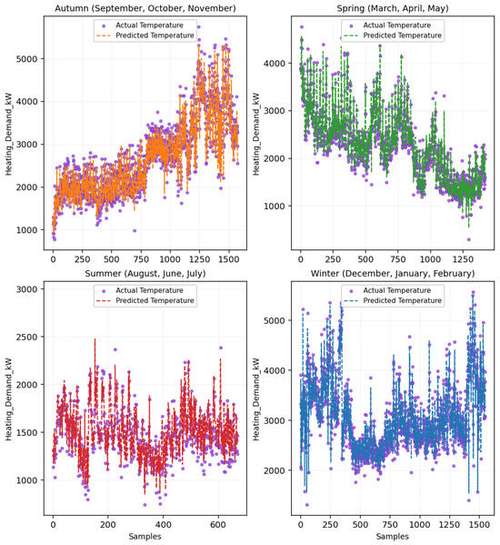
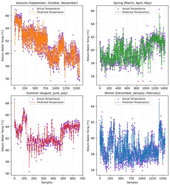
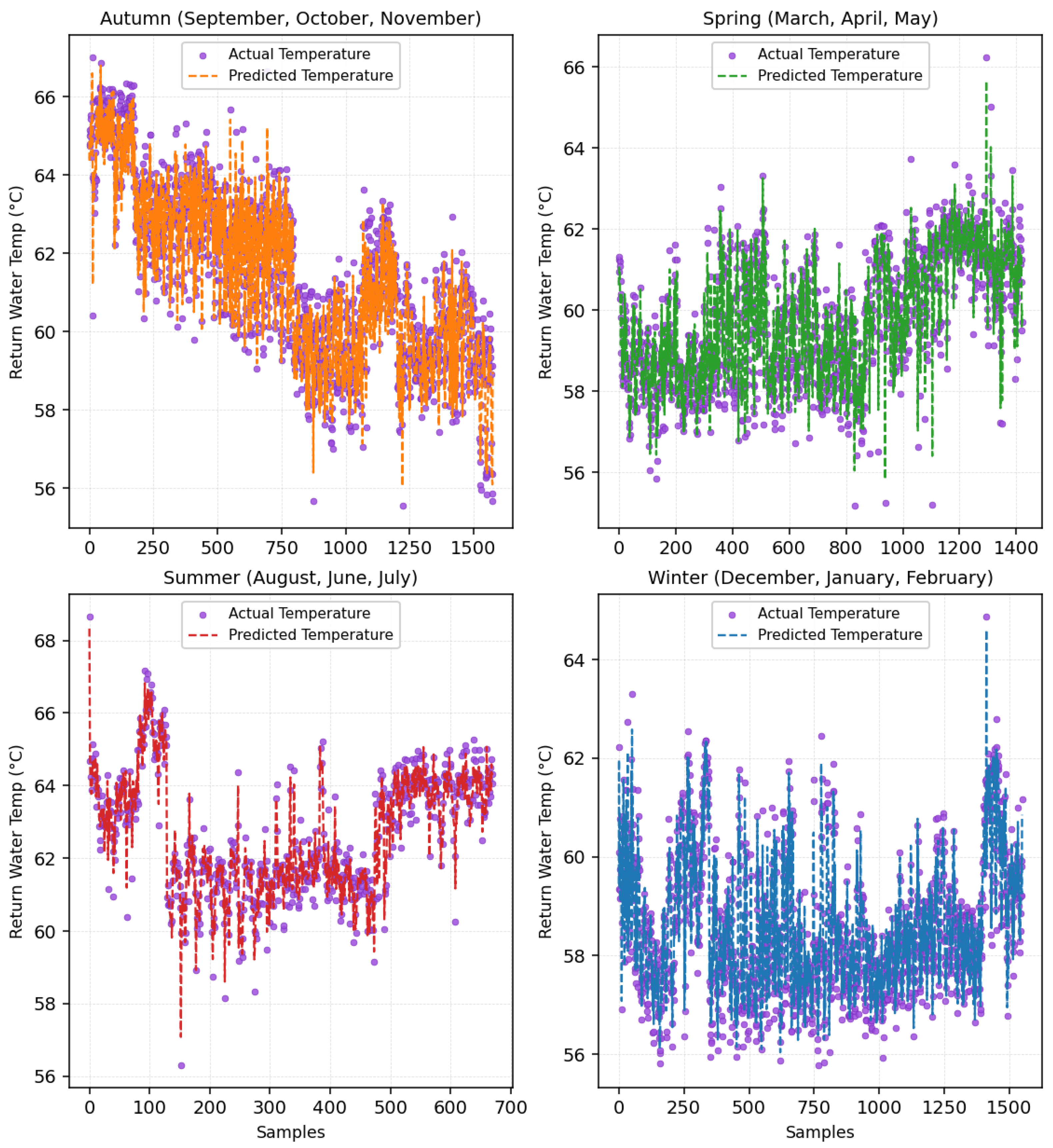
To further examine model behavior beyond aggregate error metrics, seasonal time-series predictions were analyzed for the reduced-sensor XGBoost model. Figure 4 presents the seasonal comparison between measured and predicted heating demand, while Figure 5 shows the corresponding seasonal predictions for return water temperature. Across all seasons, the model captures the dominant temporal trends and operational variability, with higher heating demand and increased fluctuations observed during winter months and more stable behavior during summer operation. The close alignment between predicted and measured values in both figures demonstrates that the reduced-sensor configuration preserves predictive fidelity across varying seasonal conditions for both thermal load and return water temperature.
Figure 4.
Seasonal prediction of heating demand using XGBoost (reduced-sensor).
Figure 5.
Seasonal prediction of return water temperature using XGBoost (reduced-sensor).
Table 8 and Table 9 summarize the results of the progressive weather feature ablation for the XGBoost model. Starting from the OAT-only baseline, adding time-based features (hour of day and day type) yields a reduction in the normalized RMSE for both heating demand and return water temperature, confirming the importance of operational schedule effects. The subsequent inclusion of humidity and barometric pressure results in consistent but smaller performance improvements, indicating that these variables provide a complementary environmental context beyond outdoor temperature alone. In contrast, the incremental gains associated with wind speed and wind direction are modest, producing marginal reductions in the normalized RMSE on the order of 0.01 or less relative to the OAT-plus-time baseline. This suggests that, while wind-related variables are not purely noise, their contribution to the prediction accuracy is secondary compared to temperature and schedule effects for this facility.
Table 8.
Stepwise weather feature ablation results for heating demand (XGBoost, normalized RMSE).
Table 9.
Stepwise weather feature ablation results for return water temperature (XGBoost, normalized RMSE).
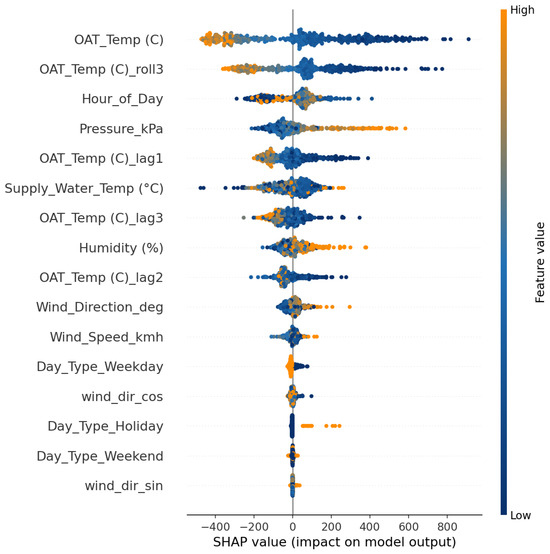
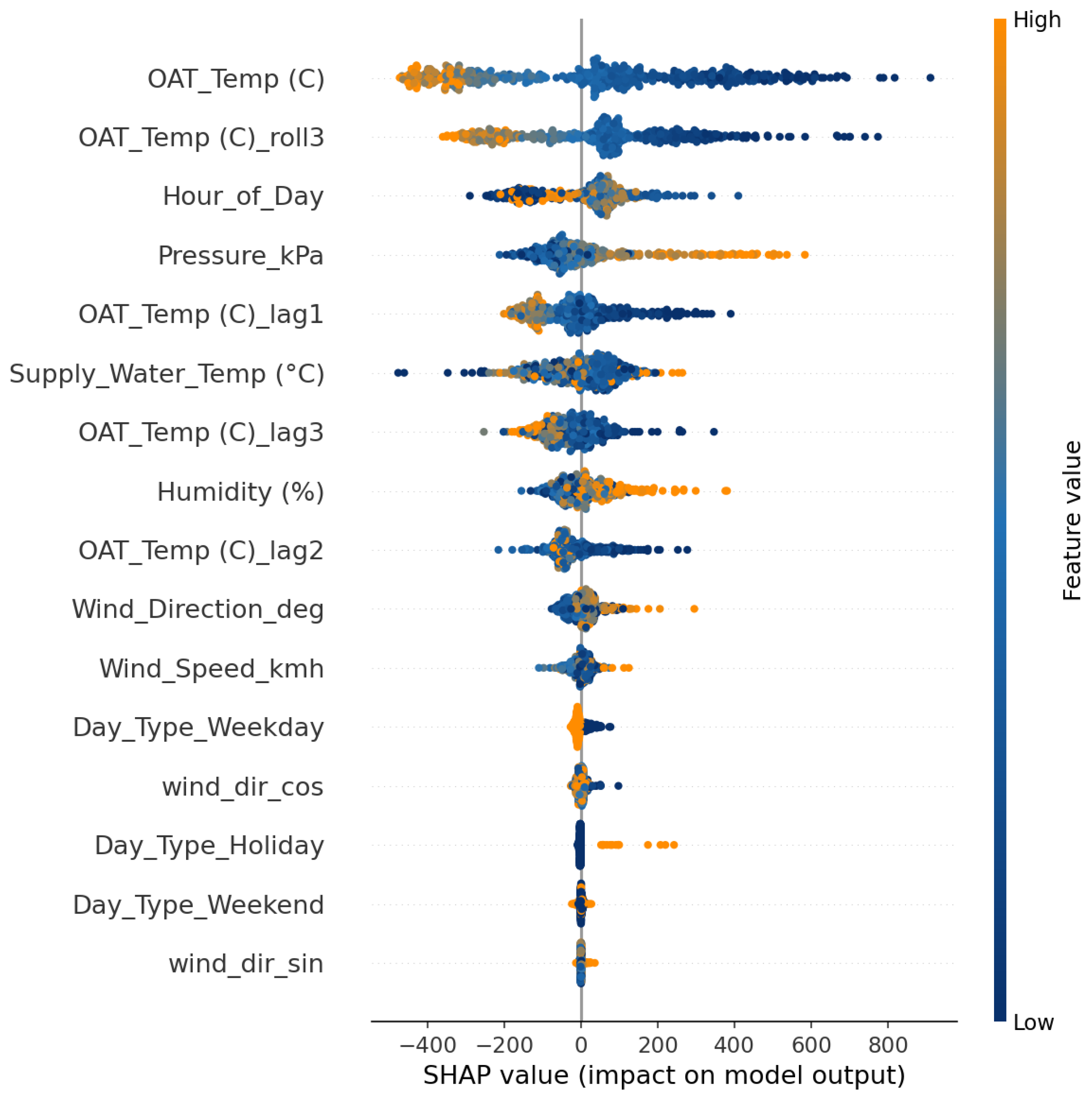
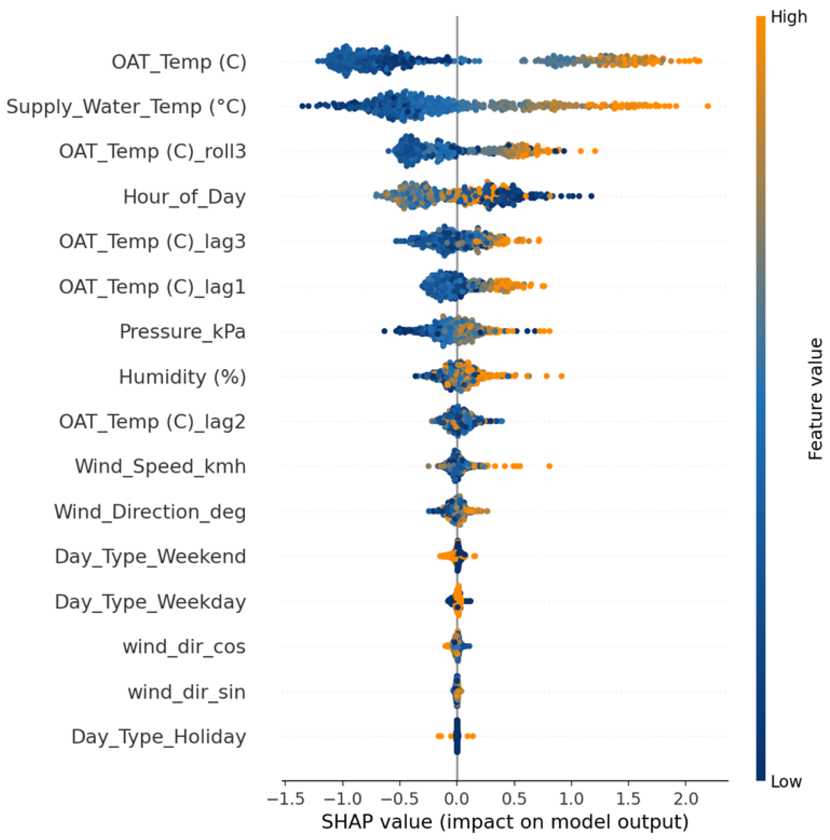
The SHAP results for heating demand show a coherent trend across both scenarios (Figure 6 and Figure 7). In the full-input configuration, flow rate and outdoor air temperature (OAT) stand out as the two dominant predictors, with flow rate having a marginally greater influence. The distribution of SHAP values for OAT behaves as expected, in which lower outdoor temperatures correspond to a higher predicted heating demand, whereas higher OATs led to smaller values. Other operational factors, including the pump VFD speed and supply water temperature, contribute to the model’s output but to a lesser extent. Time-related variables such as the hour of the day and day of the week carry relatively minor importance, since demand variations are already captured through direct operational signals like flow and temperature.
Figure 6.
Feature importance analysis using SHAP for heating demand prediction (kW) (XGBoost, full-dataset).
Figure 7.
Feature importance analysis using SHAP for heating demand prediction (kW) (XGBoost, reduced-sensor).
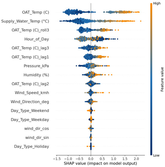
When flow-related measurements (VFD, flow rate) are removed in the reduced-input model, the relative importance of several variables shifts. OAT remains the primary driver, while hour of day gains importance as a proxy for occupancy and schedule effects. The SHAP distribution for hour of day indicates that the time-related effects, with certain hours contributing positively and others negatively to heating demand, are consistent with daily operational and occupancy patterns. Interestingly, the overall range of SHAP values for OAT becomes slightly narrower in the reduced scenario, suggesting that without detailed sensor data the model’s variability in predictions decreases. Day type features contribute very little, and no other variables emerge as dominant, indicating that the reduced model still relies on physically meaningful inputs, mainly outdoor temperature and daily timing, to infer heating demand.
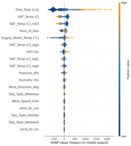
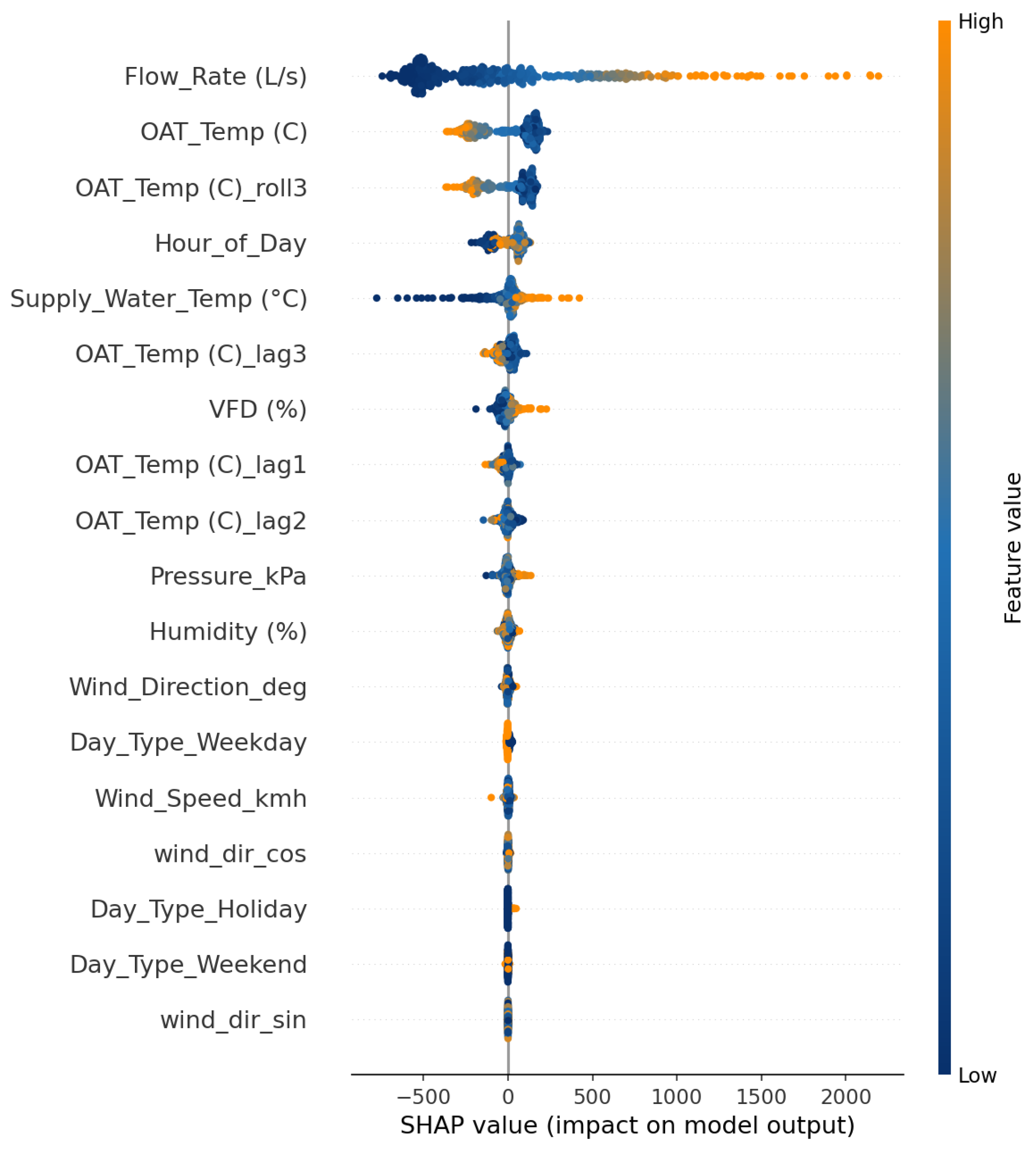
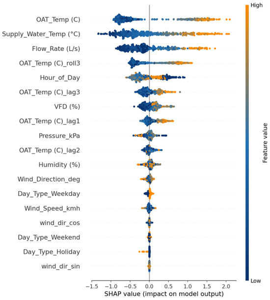
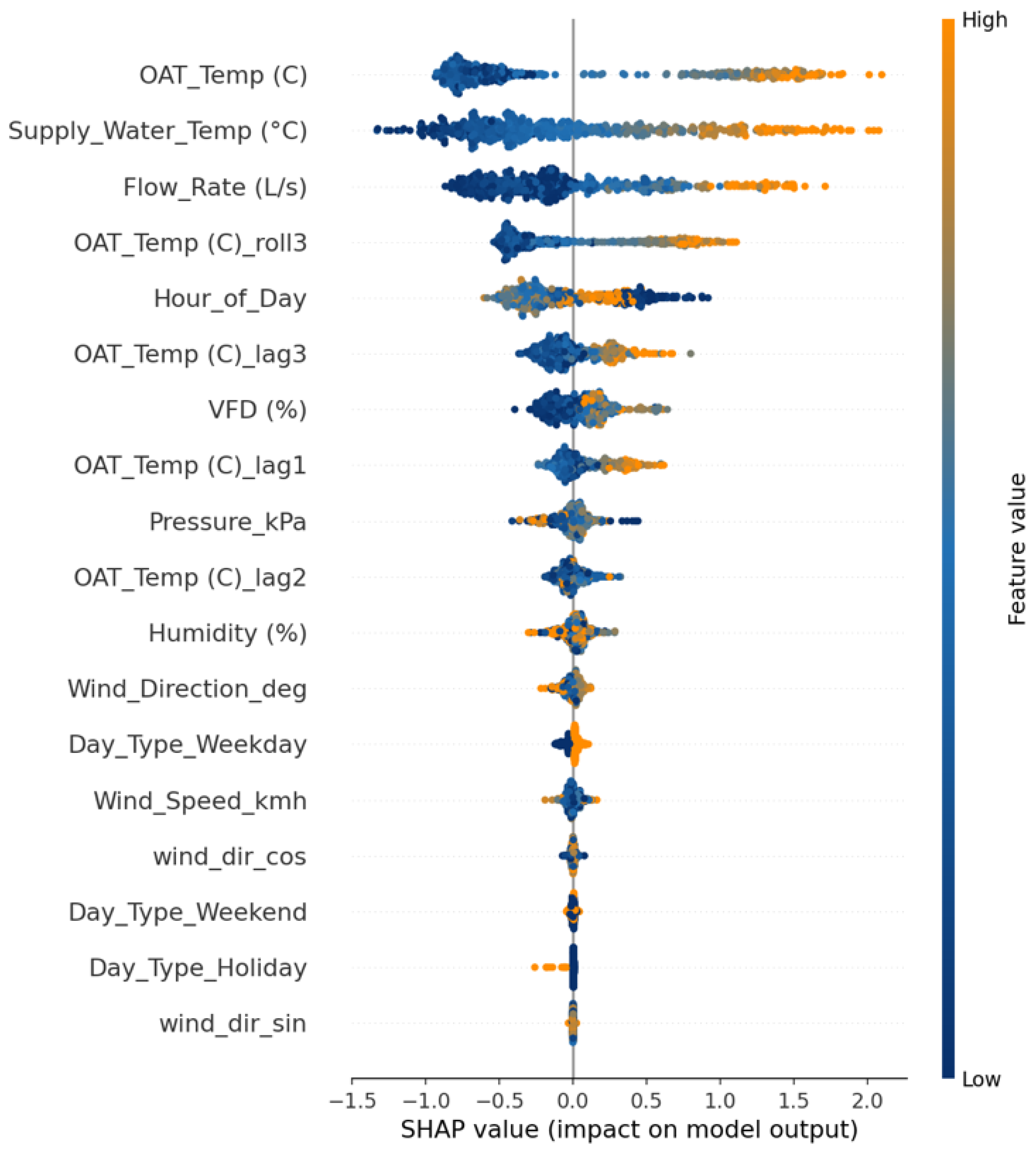
The SHAP analysis for return water temperature in Figure 8 and Figure 9 demonstrates similar insights. In the full-input scenario, OAT again emerges as the top factor, just ahead of flow rate. The relationships are intuitive, in which higher flow and colder outdoor air both correspond to lower SHAP values, meaning the return water cools when the system is delivering more heat. Warmer conditions and lower flow have the opposite effect. Control variables, including the supply water temperature, also contribute, showing that the model effectively combines environmental and operational information.
Figure 8.
Feature importance analysis using SHAP for return water temperature prediction (XGBoost, full-dataset).
Figure 9.
Feature importance analysis using SHAP for return water temperature prediction (XGBoost, reduced-sensor).
In the reduced-input RWT model, the absence of direct plant measurements causes OAT to dominate even more strongly, while the hour of day rises in importance as an indirect indicator of load. Cold outdoor conditions continue to reduce the predicted RWT, and certain hours, typically those associated with higher heating use, show more negative SHAP effects. The SHAP spread for OAT remains roughly the same or slightly narrower compared to the full model, implying a consistent influence rather than an exaggerated dependence. Overall, both targets show that, when detailed plant data are available, the models distribute importance across weather, control, and flow variables, and, when such data are limited, they fall back on the strongest and most interpretable predictors, such as outdoor temperature and time-of-day patterns.
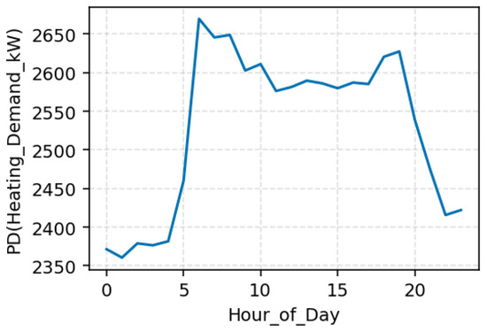
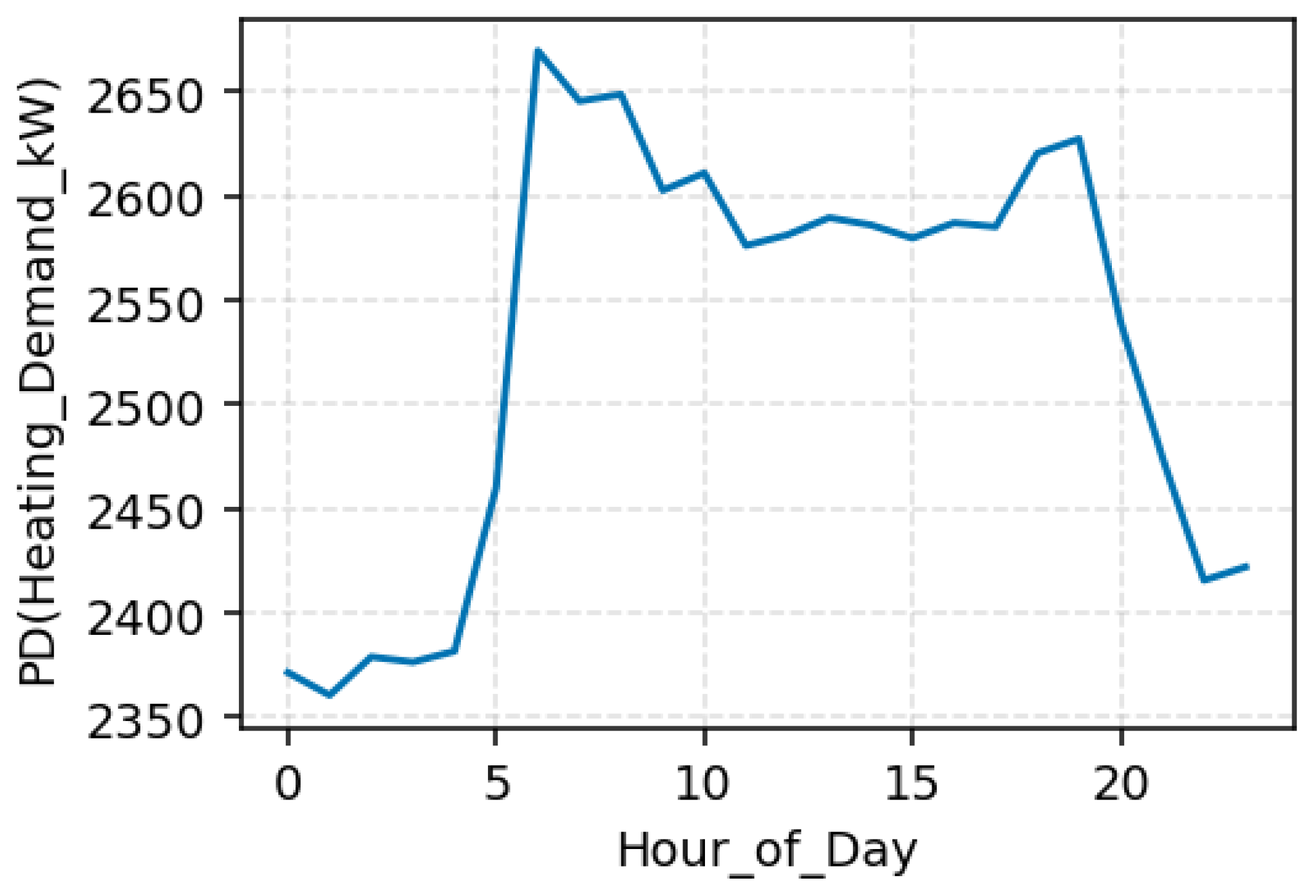
Figure 10 illustrates how predicted heating demand varies throughout the day. The model captures a clear daily rhythm: the demand is lowest overnight (around 00:00–05:00), rises sharply before dawn as the hospital warms up for occupancy, and peaks near 06:00–07:00. After this morning surge, the heating demand gradually declines through midday and levels off at moderate daytime values, with a smaller evening rise before decreasing again overnight. This curve reflects normal building operation, intensive heating during morning start-up, steady conditions while spaces remain occupied, and reduced load once activity slows. The amplitude of this daily swing is about 10 to 15 percent between nighttime lows and morning highs, highlighting when the system experiences its heaviest and lightest loads.
Figure 10.
PDP illustrating the effect of hour of day on predicted heating demand (kW) using the reduced XGBoost model excluding flow-related features.
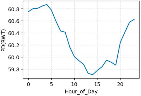
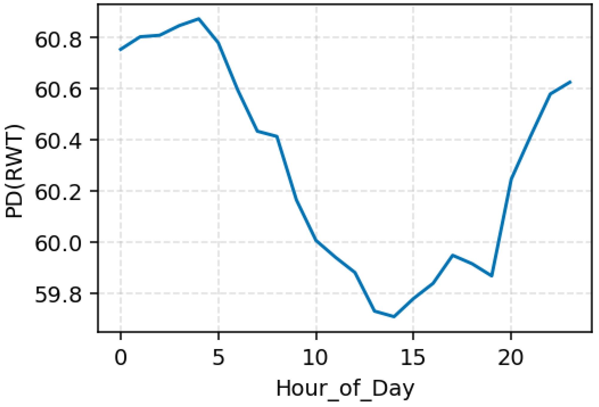
Figure 11 shows that the RWT follows an opposite pattern to the heating demand. The RWT is highest late at night and early in the morning, when the heating load is minimal and less heat is drawn from the loop, and it falls steadily throughout the morning as the system operates under sustained demand. The lowest values appear around midday to early afternoon, when continuous heat delivery cools the return water, before gradually recovering in the evening. Together, these results confirm that the hour of day acts as an effective proxy for operational schedules and occupancy in the reduced-input models. Even without direct flow or pump data, the model learns the building’s routine, anticipating the morning ramp-up, midday steady operation, and nighttime setback, which demonstrate that temporal features alone can capture much of the plant’s daily heating behavior.
Figure 11.
PDP illustrating the effect of hour of day on predicted return water temperature using the reduced XGBoost model excluding flow-related features.
5. Discussion
The results of this modeling study demonstrate the strong capability of machine learning models, particularly tree-based ensembles, to predict key heating plant variables while also offering interpretability through PDP and SHAP analyses. Both XGBoost and Random Forest performed well at capturing the relationships governing heating demand and return water temperature. XGBoost’s outperformance aligns with its reputation for handling complex nonlinear functions. However, Random Forest’s comparable performance underscores that even simpler ensemble models are sufficient to model the dominant factors of a system like this hospital’s heating plant. Furthermore, the seasonal evaluation confirms that the model performance is consistent over time; the models did not overfit to a particular season or regime. This generalization is crucial for deployment in real facility management, as it means that the model will not fail when conditions change.
Moreover, the results clearly indicate that the proxy approach was largely successful. The reduced-input models experienced only a moderate drop in accuracy, demonstrating that the time of day and similar features do capture a significant portion of the variance in heating demand and return temperature. This finding has a practical significance which suggests that, in buildings where sensor data might be sparse or temporarily unavailable, one can still obtain useful predictions by relying on schedule information and weather data. In our hospital case, the consistency of daily operations is reflected well by the hour-of-day feature, which the models utilized effectively. The SHAP analysis reinforced this, as the hour of day became a major contributor in the absence of flow sensors; this validates the hypothesis that time features can serve as effective proxies for certain operational variables in load prediction problems. One might even argue that the reduced model’s performance being close to the full model suggests some redundancy in the original feature set, as weather and time already explained most of the variance that the flow/VFD sensor was providing. This could imply that, for heating demand in this facility, the schedule and outdoor temperature are the primary drivers, and the real-time flow rate fine-tunes the prediction but does not fundamentally change it.
The use of PDP and SHAP tools also provided insight into the model. The PDP for the hour of day showed a clear and intuitive pattern in which heating demand rises in the early morning as the building warms up and stays higher during active hours, then falls overnight when occupancy and system operation decline. This smooth and consistent relationship suggests that the model has learned a realistic daily cycle rather than reacting to random noise or overfitting small fluctuations. It also serves as a quick validation that the predictions correspond with an operational point of view. Similarly, the SHAP results confirmed that the most influential features align with engineering intuition. Outdoor temperature was the top driver for both targets, which is logical given that outside conditions largely dictate heating needs. In the heating demand model, SHAP also highlighted the significance of the flow rate (full model) and time of day (reduced model), both of which have a clear explanatory meaning; the flow rate directly measures load, and the time of day captures routine load variation. There were no inexplicable top features, such as an unrelated sensor or an artifact of data collection, which sometimes can happen in black-box models. The absence of such anomalies in the interpretability analysis implies that the model focused on the right relationships. This kind of transparency is invaluable for stakeholders like facility engineers, and it transforms the model from a mysterious algorithm into a set of understandable rules. By explaining individual predictions, we could also investigate any outliers or errors. In our study, we did not encounter rigorous errors, but if there were days with larger prediction gaps, examining SHAP values could reveal whether the model was over-reliant on a particular feature or if an unmodeled factor (like an equipment malfunction) was at play. Indeed, the interpretability techniques ensured the model’s credibility and provided assurance that the model’s reasoning is aligned with real system behavior, which is crucial for adopting ML models in a critical infrastructure like a hospital energy system.
From a practical deployment perspective, the proposed framework is not intended to replace existing building management systems (BMSs), but rather to operate as a supervisory analytics layer that complements standard control architectures. While most current BMS platforms do not natively embed advanced machine learning models or digital-twin emulators, they routinely expose the operational data streams required for such analyses. Weather data, although not always directly integrated within legacy BMSs, are readily available through standard application programming interfaces and are commonly used in external energy analytics platforms. As such, the proposed approach is compatible with current hospital automation infrastructures without requiring intrusive control system modifications.
6. Conclusions
This study developed an explainable, reduced-sensor modeling framework for a hospital heating plant that combines BAS and weather data with physics-guided features to predict return water temperature and heating demand. Using XGBoost as the best-performing model, the approach maintained a strong accuracy even when high-value sensors such as flow were removed, showing that reliable insights can be derived from routinely available data. The SHAP and PDP analyses helped explain model behavior and revealed which inputs most strongly influenced performance, translating the results into practical guidance for metering priorities and control strategies. The findings suggest that data-driven, explainable models can support energy-efficient operation in hospitals without requiring new instrumentation. The work provides a practical foundation for future digital-twin development and highlights that, even with limited sensing, meaningful predictive and interpretive capabilities can be achieved for real-world building systems.
Although the model performed well across most conditions, some limitations should be acknowledged. According to the seasonal time series results, the model captured normal operating periods accurately but was less effective during extreme conditions, such as very low outdoor temperatures or sudden high heating demands. In these cases, the predictions tended to underestimate peaks, especially in winter, which is reasonable given that the reduced-sensor setup excluded the flow signal that normally reflects rapid load changes. The analysis was also limited to one hospital plant with a specific control strategy and climate, so the results may vary for other facilities; additional studies to validate this approach across multiple buildings are planned to address this issue.
Despite its strong predictive performance, the XGBoost model has several notable limitations. As a data-driven approach, its accuracy depends on the representativeness of the training data and may degrade under operating conditions not observed historically. While the model captures complex nonlinear relationships, it does not explicitly enforce physical constraints, which can limit extrapolation under extreme or abnormal conditions. Additionally, the data contained inherent sensor uncertainty and occasional noise, which could have influenced the model accuracy; future work should integrate sub-hourly data to better capture fast transients and add uncertainty estimation to improve confidence in predictions. Exploring low-cost proxy sensors or hybrid physics–data models could also help enhance accuracy during extreme or rapid operational changes.
Author Contributions
Conceptualization, M.F. and J.J.M.; methodology, M.F. and J.J.M.; software, M.F.; validation, M.F. and J.J.M.; formal analysis, M.F.; investigation, M.F.; data curation, M.F.; visualization, M.F.; writing—original draft preparation, M.F.; writing—review and editing, M.F. and J.J.M.; supervision, J.J.M.; project administration, J.J.M.; funding acquisition, J.J.M. All authors have read and agreed to the published version of the manuscript.
Funding
This research was funded by the Natural Science and Engineering Research Council (ALLRP 580958-2022) and H.H. Angus and Associates.
Data Availability Statement
The data used in this study are not publicly available due to confidentiality agreements with the partner hospital and the sensitive nature of BAS operational records.
Conflicts of Interest
The authors declare no conflicts of interest, and the sponsors had no role in the design, analysis, or publication of this work.
References
- Liang, J.; Gau, H.; Chen, K.; Yu, K.; Caitong, Y.; Yunpeng, M. A Survey on Intelligent Optimization Approaches to Boiler Combustion Optimization. CAAI Artif. Intell. Res. 2023, 2, 9150014. [Google Scholar] [CrossRef] [Scilit]
- Tian, Z.; Wei, S.; Shi, X. Developing data-driven models for energy-efficient heating design in office buildings. J. Build. Eng. 2020, 32, 101778. [Google Scholar] [CrossRef] [Scilit]
- Bawaneh, K.; Farnaz, G.N.; Rasheduzzaman, M.; Deken, B. Energy Consumption Analysis and Characterization of Healthcare Facilities in the United States. Energies 2019, 12, 3775. [Google Scholar] [CrossRef] [Scilit]
- Panagiotou, D.K.; Dounis, A.I. Comparison of Hospital Building’s Energy Consumption Prediction Using Artificial Neural Networks, ANFIS, and LSTM Network. Energies 2022, 15, 6453. [Google Scholar] [CrossRef] [Scilit]
- Coccagna, M.; Cesari, S.; Valdiserri, P.; Romio, P.; Mazzacane, S.; Coccagna, M. Energy consumption in hospital buildings: Functional and morphological evaluations of six case studies. Int. J. Environ. Sci. 2017, 2, 443–452. [Google Scholar]
- Shen, C.; Zhao, K.; Ge, J.; Zhou, Q. Analysis of building energy consumption in a hospital in the hot summer and cold winter area. Energy Procedia 2019, 158, 3735–3740. [Google Scholar] [CrossRef] [Scilit]
- Fraile, J.-C.; San-José, J.; Ana, G.-A. A boiler room in a 600-bed hospital complex: Study, analysis, and implementation of energy efficiency improvements. Energies 2014, 7, 3282–3303. [Google Scholar] [CrossRef] [Scilit]
- Stock, M.; Kandil, M.; Macleod, B.; Pilgrim, B.; McArthur, J. HVAC performance evaluation and optimization algorithms development for large buildings. Build. Simul. 2021, 17, 3080–3087. [Google Scholar]
- Nemitallah, M.A.; Nabhan, M.A.; Alowaifeer, M.; Haeruman, A.; Alzahrani, F.; Habib, M.A.; Elshafei, M.; Abouheaf, M.I.; Aliyu, M.; Alfarraj, M. Artificial intelligence for control and optimization of boilers’ performance and emissions: A review. J. Clean. Prod. 2023, 417, 138109. [Google Scholar] [CrossRef] [Scilit]
- Saloux, E.; Runge, J.; Zhang, K. Operation optimization of multi-boiler district heating systems using artificial intelligence-based model predictive control: Field demonstrations. Energy 2023, 285, 129524. [Google Scholar] [CrossRef] [Scilit]
- Prabhu, V.; Chaudhary, D. Machine Learning enabled Condition Monitoring Models for Predictive Maintenance of Boilers. In Proceedings of the 2021 4th International Conference on Recent Developments in Control, Automation & Power Engineering (RDCAPE), Noida, India, 7–8 October 2021. [Google Scholar]
- You, D.; Tan, X.; Liu, Z.; Li, D.; Wang, Z. Energy saving and carbon reduction schemes for hospital with photovoltaic power generation and system upgrading technology. Heliyon 2023, 9, e21447. [Google Scholar] [CrossRef] [Scilit]
- Agarwal, M.; Cameron-Rastogi, P.; Peronato, G.; Mavromatidis, G. Missed opportunities in building energy performance assessment. J. Sustain. Real Estate 2024, 16, 2387486. [Google Scholar] [CrossRef] [Scilit]
- Qiao, Q.; Yunusa-Kaltungo, A.; Edwards, R.E. Feature selection strategy for machine learning methods in building energy consumption prediction. Energy Rep. 2022, 8, 13621–13654. [Google Scholar] [CrossRef] [Scilit]
- Fatehijananloo, M.; Stopps, H.; McArthur, J. Exploring artificial intelligence methods for energy prediction in healthcare Facilities: An In-Depth extended systematic review. Energy Build. 2024, 320, 114598. [Google Scholar] [CrossRef] [Scilit]
- Yao, Z.; Romero, C.; Baltrusaitis, J. Combustion optimization of a coal-fired power plant boiler using artificial intelligence neural networks. Fuel 2023, 344, 128145. [Google Scholar] [CrossRef] [Scilit]
- Ye, T.; Dong, M.; Long, J.; Zheng, Y.; Liang, Y.; Lu, J. Multi-objective modeling of boiler combustion based on feature fusion and Bayesian optimization. Comput. Chem. Eng. 2022, 165, 107913. [Google Scholar] [CrossRef] [Scilit]
- Zor, K.; Çelik, Ö.; Timur, O.; Teke, A. Short-Term Building Electrical Energy Consumption Forecasting by Employing Gene Expression Programming and GMDH Networks. Energies 2020, 13, 1102. [Google Scholar] [CrossRef] [Scilit]
- Thota, S.; Syed, M.B. Analysis of feature selection techniques for prediction of boiler efficiency in case of coal based power plant using real time data. Int. J. Syst. Assur. Eng. Manag. 2024, 15, 300–313. [Google Scholar] [CrossRef] [Scilit]
- Balali, Y.; Chong, A.; Busch, A.; O’Keefe, S. Energy modelling and control of building heating and cooling systems with data-driven and hybrid models—A review. Renew. Sustain. Energy Rev. 2023, 183, 113496. [Google Scholar] [CrossRef] [Scilit]
- Nikula, R.-P.; Ruusunen, M.; Leiviskä, K. Data-driven framework for boiler performance monitoring. Appl. Energy 2016, 183, 1374–1388. [Google Scholar] [CrossRef] [Scilit]
- Amasyali, K.; El-Gohary, N.M. A review of data-driven building energy consumption prediction studies. Renew. Sustain. Energy Rev. 2018, 81, 1192–1205. [Google Scholar] [CrossRef] [Scilit]
- Cao, L.; Li, Y.; Zhang, J.; Jiang, Y.; Han, Y.; Wei, J. Electrical load prediction of healthcare buildings through single and ensemble learning. Energy Rep. 2020, 6, 2751–2767. [Google Scholar] [CrossRef] [Scilit]
- Ruiz, E.; Pacheco-Torres, R.; Casillas, J. Energy consumption modeling by machine learning from daily activity metering in a hospital. In Proceedings of the 2017 22nd IEEE International Conference on Emerging Technologies and Factory Automation, Limassol, Cyprus, 12–15 September 2017; pp. 1–7. [Google Scholar]
- Ahmed, N.; Bennati, S.; Anglani, N. Energy Performance Benchmarking and Indicators: A Comprehensive Framework for Scientifically Sound Data-Driven and Energy Management Improvements in Hospitals. In Proceedings of the 2024 IEEE 8th Energy Conference (ENERGYCON), Doha, Qatar, 4–7 March 2024; pp. 1–6. [Google Scholar]
- Wang, H.; Wen, W.; Zhang, Z.; Gao, N. Construction of building energy consumption prediction model based on multi-optimization model. Buildings 2023, 13, 1677. [Google Scholar] [CrossRef] [Scilit]
- Chen, Z.; Xiao, F.; Guo, F.; Yan, J. Interpretable machine learning for building energy management: A state-of-the-art re-view. Adv. Appl. Energy 2023, 9, 100123. [Google Scholar] [CrossRef] [Scilit]
- Manfren, M.; Gonzalez-Carreon, K.M.; James, P.A. Interpretable data-driven methods for building energy modelling—A review of critical connections and gaps. Energies 2024, 17, 881. [Google Scholar] [CrossRef] [Scilit]
- Henkel, P.; Kasperski, T.; Stoffe, P.; Müller, D. Interpretable data-driven model predictive control of building energy systems using SHAP. In Proceedings of the 6th Annual Learning for Dynamics & Control Conference, Oxford, UK, 15–17 July 2024; pp. 222–234. [Google Scholar]
- Moon, J.; Maqsood, M.; So, D.; Baik, S.W.; Rho, S.; Nam, Y. Advancing ensemble learning techniques for residential building electricity consumption forecasting: Insight from explainable artificial intelligence. PLoS ONE 2024, 19, e0307654. [Google Scholar] [CrossRef] [Scilit]
- Lundberg, S.M.; Lee, S.-I. A unified approach to interpreting model predictions. Adv. Neural Inf. Process. Syst. 2017, 30, 4768–4777. [Google Scholar]
- Shahcheraghian, A.; Ilinca, A. Advanced machine learning techniques for energy consumption analysis and optimization at UBC Campus: Correlations with meteorological variables. Energies 2024, 17, 4714. [Google Scholar] [CrossRef] [Scilit]
- Shakeel, H.M.; Iram, S.; Hill, R.; Farid, H.M.A.; Sheikh-Akbari, A.; Saleem, F. A Machine Learning-Based Intelligent Framework for Predicting Energy Efficiency in Next-Generation Residential Buildings. Buildings 2025, 15, 1275. [Google Scholar] [CrossRef] [Scilit]
- Cappelli, F.; Castronuovo, G.; Grimaldi, S.; Telesca, V. Random forest and feature importance measures for discriminating the most influential environmental factors in predicting cardiovascular and respiratory diseases. Int. J. Environ. Res. Public Health 2024, 21, 867. [Google Scholar] [CrossRef] [Scilit]

Disclaimer/Publisher’s Note: The statements, opinions and data contained in all publications are solely those of the individual author(s) and contributor(s) and not of MDPI and/or the editor(s). MDPI and/or the editor(s) disclaim responsibility for any injury to people or property resulting from any ideas, methods, instructions or products referred to in the content. |
© 2026 by the authors. Licensee MDPI, Basel, Switzerland. This article is an open access article distributed under the terms and conditions of the Creative Commons Attribution (CC BY) license.