


Abstract
Winkler models transmit no shear and cannot reproduce the differential settlement and lateral squeezing that drive soft-ground widening distress. The Pasternak model restores shear coupling, but its shear layer stiffness has remained unmeasurable without static loading. This study identified the compression coefficient k and shear layer stiffness from lightweight plate vibration tests. A Hamiltonian eigenvalue formulation distinguished the parameters through their different geometric weights in the fundamental mode; a Chebyshev–Ritz solver established internal convergence, with independent verification by a SAP2000 v27 solid model against laboratory frequencies. Bayesian MCMC with a K30-informed prior and a resolution-consistent noise model returned k = 5.99 ± 0.58 MPa/m and = 0.153 ± 0.008 MN/m, with prior sensitivity and leave-one-plate-out checks. Transferred to Abaqus 2026 and SAP2000 v27 without retuning, the model agreed with a published finite element benchmark—a consistency check, not a field validation—within 5% on the shear-driven responses, whereas a matched-stiffness Winkler model deviated by roughly 20%. Recalibrating the Winkler stiffness closed that gap only by shifting the stiffness estimate by approximately two posterior standard deviations from the identified value, and the trough extent remained unreproduced. The Sobol indices indicated that these responses were driven primarily by . A three-plate campaign can be completed within one working day without requiring lane closure; field instrumentation is under way.
1. Introduction
1.1. Framing the Widening Problem
Expressways across the Yangtze River Delta and the adjacent alluvial plains are being widened systematically from four to eight lanes. Widening changes how existing embankment works: the new fill loads only part of the cross-section, so the embankment shifts from one-dimensional compression toward a three-dimensional stress state in which differential settlement and lateral squeezing develop while the underlying soft deposits continue to consolidate for years. Centrifuge tests by Allersma, Ravenswaay, and Vos [1] show that widening on such soils induces longitudinal cracking and shoulder drop-off, with overlay fatigue accumulating over time. Field measurements by Lin, Zhang, and Zhang [2] point in the same direction: the vibration response of soft-soil foundations concentrates at low frequencies, close to resonance under traffic loading. These distress modes are transmitted through shear in the foundation and eventually manifest as maintenance liability, which makes the choice of foundation model the controlling assumption of any widening analysis [3].
Foundation models form a hierarchy—Winkler, two-parameter, and continuum—each step relaxing the assumptions about mechanical coupling within the support medium [4]. Winkler’s model [5], in which the reaction depends exclusively on the local displacement, has served geotechnical practice for over a century, but its uncoupled springs do not transmit shear: the settlement trough terminates abruptly at the load perimeter, and no stress crosses the old–new embankment interface [6,7]. The Pasternak model addresses this defect by interposing a shear layer between the spring bed and the superstructure, so that the reaction at any point depends on the spatial gradients of the deflection rather than on the deflection alone [8,9]. One of its two parameters governs compressive strain and the other shear strain, and both must be known before the model can be used [4].
The Pasternak model fits the widening problem mechanically; what has prevented its routine use is that its two parameters resist measurement. A static plate load test returns a single equivalent stiffness, from which the compression coefficient k and the shear layer stiffness cannot be decoupled; Terzaghi [10] recognized this limitation, and back-analysis of settlement records fares no better, being ill-conditioned and noise-sensitive [11]. The difficulty is as practical as it is theoretical: geogrid interlayers or cement deep mixing can be ranked against differential settlement only when both parameters are known [12]. Carbon has joined cost as a constraint: carbon accounting studies of ground investigation [13,14] document appreciable emissions from conventional testing campaigns, most of them from heavy plant and lane closures, which favors lighter procedures (the preliminary, assumption-transparent estimate of Appendix D is 1.5–2.4 t CO2e avoided per site). The problem is also not confined to highways: the same two-parameter idealization underlies the rafts and mat foundations of buildings on soft deposits [3], so an identification route developed for widening corridors carries over to building foundation assessment as well.
1.2. Assessing Prior Identification Routes
The forward problem—predicting natural frequencies from known foundation parameters—rests on established theory. Hamilton’s principle supplies the variational basis [3,4], and mature solvers furnish independent numerical checks, from shear-deformation plate solutions on Winkler–Pasternak–Kerr foundations [15] to Rayleigh–Ritz procedures for laminated plates on two-parameter foundations [16,17,18] and global-mode frequency surfaces for beams [11]. These studies, however, treat the parameters as known inputs; how they should be measured is left open.
The inverse problem—recovering the parameters from measured frequencies—is where the difficulties concentrate. Yao et al. [11] identified beam foundation stiffness from global modes and time-domain subspace models, but the result is a point estimate with no uncertainty attached. Bayesian formulations close that gap by returning posterior distributions: Shirzad-Ghaleroudkhani et al. [19] updated the soil–foundation stiffness of buildings on sway and rocking springs, and Gibbs-sampling schemes have extracted modal properties from noisy seismic and ambient records [20,21,22]. Nevertheless, none of these schemes can separate two foundation parameters, and the reason is structural rather than numerical: their forward models lump the soil into one stiffness per response mode—a sway spring, a rocking spring, a modal stiffness—so compression and shear effects merge into a single equivalent value that no modal data can split. The separation achieved here is possible only because the plate forward model supplies two distinct geometric weights (Equation (8)); it does not extend to building-type soil–structure systems without an analogous multi-weight forward model. The deterministic Powell inversion of Zhang et al. [23] estimated a single Winkler coefficient and likewise stops short of a two-dimensional parameter space.
A related line of work replaces explicit mechanics with learned models: physics-informed and thermodynamics-informed networks solve forward and inverse problems and enforce physical laws within learned constitutive models [24,25,26,27]. For the present problem two gaps remain: calibration from element-level tests to field boundary-value problems is unresolved [28], and parameter recovery still relies on triaxial or oedometer programs rather than in situ dynamic measurements [29,30,31]. Digital-twin pipelines have advanced to real-time control and risk prognosis in tunneling and deep excavation [32,33,34,35], but they consume foundation parameters rather than produce them.
Cross-platform checking addresses a different risk: identified parameters may be artifacts of the identification model rather than properties of the soil. Shaker tests on offshore monopiles found model-dependent errors of 20–140% in low-frequency soil stiffness [36], and related work has extracted soil–foundation stiffness and boundary conditions from the vibration of bridge substructures [37,38]. Verification on an independently coded platform is, therefore, an essential control on modeling error.
Closest to the present problem, quasi-Newton inversion has reconciled field measurements with generalized Pasternak models of slabs on grade [39], classical impedance formulas supply dynamic benchmarks [40], and caisson foundations have been identified from in situ vibration with simplified mass–spring–dashpot models [41]. The decade review of Hou and Xia [42], however, finds that vibration-based identification still hinges on iterative forward solutions, and these routes either embed the mechanics in a surrogate or return point values without uncertainty. The method developed below targets precisely that combination: explicit mechanics, a posterior distribution rather than a point value, and a forward model fast enough to serve the monitoring pipeline of Section 9.
1.3. Contributions and Paper Structure
The starting point is that the compression coefficient k and the shear layer stiffness enter the dynamic equations of a vibrating plate with different geometric weights, so frequency measurements alone can decouple them, with no static loading stage. The shear layer stiffness is an equivalent stiffness with units of force per unit length, derived in Section 3.1 from the material shear modulus of the layer; the two quantities are used consistently throughout the paper. The work proceeds in four stages (Figure 1): Stage I derives the forward model from Hamilton’s principle; Stage II verifies it with an independent Chebyshev–Ritz spectral solver; Stage III embeds the model in adaptive Bayesian Markov chain Monte Carlo (MCMC) inference and Sobol global sensitivity analysis; and Stage IV verifies the identified parameters against the measured dynamics on two independently coded finite-element platforms, checks them against array-measured mode shapes and assesses their consistency against a published simulation of the reference widening.
Figure 1.
The four-stage workflow of this study, from the Hamiltonian forward model to cross-platform checking. Variables passed between stages are annotated on the connecting arrows.
The contribution of this study lies not in any single ingredient, but in the coupling of three choices. First, the energy formulation is rebuilt on dimensional grounds: the shear contribution enters through the shear layer stiffness in force per unit length, which removes the inconsistency that arises when a material modulus is inserted directly into an energy functional, and its geometric weight is the Rayleigh quotient of the fundamental flexural mode shape, evaluated on simply supported analytical shapes and checked against the accelerometer array records (Section 7); the exterior field contribution that would govern a rigid punch is absorbed into the effective shear layer stiffness (Section 3.2). Second, the identification is probabilistic end to end: static K30 evidence enters as an informative prior rather than a competing point estimate, and the posterior is reported together with its prior architecture so that the influence of the deliberately weak three-plate likelihood remains visible. The sampler is the adaptive Metropolis algorithm of Haario, Saksman and Tamminen [43]; convergence is diagnosed after Gelman and Rubin [44]; and global sensitivities use the variance-based total-effect estimator of Saltelli et al. [45]. Third, the analytical, numerical and experimental frequency chains are compared on equal terms, and the settlement-level comparison draws on a published benchmark that played no role in any calibration step; method agreement follows Bland and Altman [46], and the power spectral densities of the vibration records follow Welch [47].
The dynamic plate vibration data that feed the Bayesian inversion were acquired by the authors in a controlled laboratory program [48] involving three instrumented plates on a homogeneous sand bed; the test protocol and the spectral identification procedure are presented in Section 7. For cross-platform verification, we built a high-fidelity finite element model of the reference widening in Abaqus 2026 (Section 8), using the geotechnical profile and the staged-construction sequence detailed in [49]. Because both the experimental frequencies and the numerical benchmark originate from the present research program, their provenance, and the attendant limits on external validation, are addressed explicitly in Section 10. Terminology follows that distinction throughout: the Abaqus 2026 and SAP2000 v27 checks are reported as cross-platform verification, the comparison with [49] as a benchmark consistency assessment, and validation is reserved for confrontation with independent field data.
The paper is organized as follows. Section 2 frames the engineering problem and the physical role of the two parameters, and Table 1 positions the method against existing identification routes. Section 3, Section 4, Section 5 and Section 6 present the four stages in turn: the Hamiltonian forward model, Chebyshev–Ritz spectral verification, Bayesian MCMC inference with Sobol sensitivity analysis and robustness checks, and cross-platform numerical verification. Section 7 reports the laboratory campaign, Section 8 the application against the published benchmark, and Section 9 a short deployment outlook. Section 10 discusses implications and data provenance, Section 11 collects the limitations and future work, and Section 12 concludes. Appendix A, Appendix B, Appendix C, Appendix D and Appendix E supply the dimensional derivation, the MCMC diagnostics, the finite-element setup, the carbon estimate and the interface patch test.
Table 1.
Comparison of existing identification routes for foundation stiffness parameters with the present method.
2. Engineering Background and Problem Statement
2.1. Site Conditions and Widening Geometry
The reference project is a unilateral widening of an expressway on deep soft ground in the Yangtze River Delta alluvial plain [48,49]. The subsoil profile comprises four layers to 40 m depth (Figure 2): silty clay (0–6 m), muddy silty clay (6–16 m), silty clay with sand (16–28 m) and muddy silty clay interbedded with silt sand (28–40 m), with the groundwater table 2.0 m below grade. The existing embankment is 26 m wide at the base and 3.5 m high; new shoulders of b = 4.5 m, 8.25 m and 12.5 m span the practical range of four-to-eight-lane expansion. Points A (new-embankment centerline) and B (old–new interface) mark the locations at which settlement and pore pressure are evaluated in the benchmark study [49].
Figure 2.
Engineering geological profile of the soft-ground site and geometry of unilateral highway widening: cross-section with the existing embankment, the three widening widths, the evaluation points A and B and the groundwater table (GWT). The physical properties and constitutive-model assignment of the four soil layers are listed in Table 2.
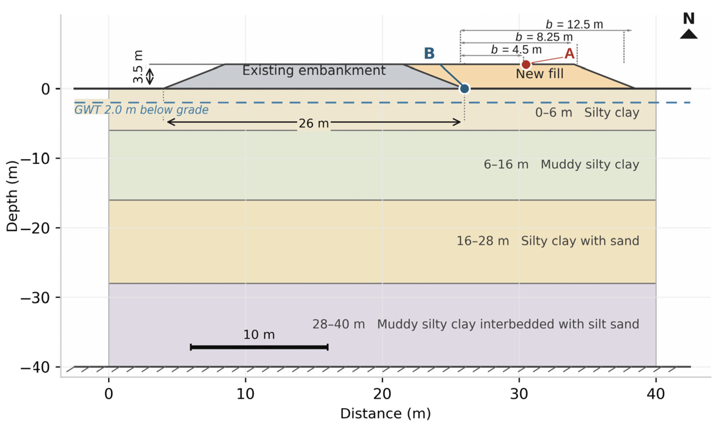
Table 2.
Representative physical properties and constitutive model assignment of the four soil layers of Figure 2 (constitutive models as specified in Section 6.1 and Table A5).
2.2. Why Two Parameters Are Necessary
The Winkler idealization relates the foundation reaction q to the local displacement w through a single coefficient of subgrade reaction, called the compression coefficient in this paper, with units of force per unit volume,
so that the reaction vanishes wherever the displacement vanishes and the settlement trough terminates abruptly at the load edge. The Pasternak idealization interposes a shear layer between the Winkler springs and the loaded surface,
in which is the shear layer stiffness of the layer, with units of force per unit length. Three stiffness quantities are used in this paper and are never interchanged: the compression coefficient (force per unit volume), the material shear modulus of the layer (force per unit area, Section 3.1) and the equivalent shear layer stiffness (force per unit length). Equation (2) transmits shear between adjacent springs, and the resulting trough extends continuously beyond the loaded area (Figure 3). For widening problems, of which the governing distress mechanism is shear transfer, this distinction is structural: a model that cannot transmit shear across the old–new interface cannot rank the interventions designed to control it. The long-standing obstacle has never been the model itself, but identifying its two parameters from measurements that are cheap, fast and lightly instrumented. Stage I takes up that obstacle.
q = kw,
Figure 3.
Mechanism comparison of the Winkler and Pasternak (two-parameter) foundation models with the corresponding normalized one-dimensional settlement troughs: (a) Winkler model (q = kw, τ = 0); (b) Pasternak two-parameter model () with the shear layer ; (c) Winkler trough terminating abruptly at the load edge because the springs carry no shear; (d) continuous Pasternak trough extending beyond the load edge and across the old–new interface.
Identifiability dictates the two-parameter formulation adopted here, rather than a richer continuum-reduced model such as the Kerr three-parameter foundation [7]. Each plate contributes a single fundamental frequency observation, and the eigenvalue equation supplies exactly two geometric weights—the contact area A weighting k and the mode-shape Rayleigh quotient λ2 weighting —so two parameters are the most that a set of plates can separate. A third foundation constant would enter through a geometric weight that is linearly dependent on the first two for the fundamental mode, making it unidentifiable from fundamental-frequency data alone; exploiting higher modes is left to future work (Section 11). The continuum end of the hierarchy is likewise covered: Section 8 benchmarks the identified two-parameter model against the coupled-consolidation continuum simulation of [49] (agreement within 4.1–4.9% on the engineering responses), and Appendix E shows that the discrete shear link implementation of the Pasternak interface reproduces the analytical settlement trough within the 5% verification tolerance, so the model is bracketed on both sides of the foundation hierarchy with its deviation from each quantified.
3. Stage I: Hamiltonian Energy-Variational Forward Model
3.1. Kinematic and Constitutive Assumptions
Consider a plate of plan dimensions a × b resting on a Pasternak foundation (Figure 4). Two assumptions are made at the outset and revisited against the results in Section 10 and Section 11. First, the plates are thick relative to their plan size, but not perfectly rigid: the fundamental vibration mode is taken to be the lowest flexural mode of the plate in free vibration, as confirmed by the three-accelerometer array on each plate (Section 7), and its shape enters the energy functional through its Rayleigh quotient. Second, the soil displacement beneath the plate decays with depth z according to a linear shape function—a first-mode approximation adopted because it closes the energy expressions analytically, not because the true displacement field is linear (its limitations are examined in Section 11). Because this mode is flexural rather than rigid-body, the plan gradients of beneath the plate do not vanish, and the shear energy in Equation (7) is non-zero by construction; the rigid-punch regime, in which the shear energy would arise solely from the exterior field, is not the regime of the present plates (Section 7.1).
where H is the effective participating depth. Following the empirical rule adopted for rigid-plate vibration on effectively unbounded soil [48], H = 3.0min(a,b) is adopted for rectangular plates and H = 3.0d for circular plates of diameter d; the value exceeds the static rule of thumb because vibration mobilizes additional soil mass through inertial coupling [48], and its influence on the identified parameters is bounded by the sensitivity analysis reported in Section 10. The rule presumes a homogeneous or mildly layered, effectively unbounded soil mass; strongly stratified or partially saturated profiles require the re-examination taken up in Section 10. In a bounded test pit the rigid walls and floor truncate the participating zone, and the effective depth becomes Heff = min[3.0min(a,b), Hpit], where Hpit is the boundary-limited participating depth of the pit (Section 7.1 and Appendix A.3).
Figure 4.
Plate–two-parameter foundation coupled system: (a) exploded view of the plate undergoing fundamental-mode vibration on the shear layer and Winkler springs; (b) linear depth-decay shape function ϕ(z) over the participating depth H.
The Pasternak shear layer deforms wherever the displacement field varies in plan: beneath the plate, where the flexural mode shape supplies the non-zero gradients, and beyond the plate perimeter, where the exterior field decays over the characteristic length . For a rigid punch, the exterior contribution would be the only one, and its boundary-integral form scales with the plate perimeter and that decay length; for the present flexural modes the interior gradients dominate the Rayleigh quotient of Equation (9), and the residual exterior contribution is absorbed into the effective shear layer stiffness. We characterize the layer by its shear layer stiffness,
where G is the material shear modulus of the layer (force per unit area) and ts its effective thickness. Introducing is required on dimensional grounds: with G alone, the shear energy density G(∇w)2 carries units of force per unit area, which cannot be added to the Winkler energy density kw2 (force per unit volume times squared length); with , both contributions integrate to work, and the functional is dimensionally closed (Appendix A). For the present site ts = 0.5 m, calibrated from the shear-wave profile and the depth of the mobilized shear zone [48]. Two interpretive consequences follow. The frequency data identify only the product , so ts cannot be separated from G without independent evidence, and the value ts = 0.5 m is adopted solely for interpretation. At the identified , the implied modulus ≈ 0.31 MPa is only about 4% of the intact small-strain modulus of the pit sand (≈8.5 MPa from E = 22 MPa with ν = 0.3): is an effective stiffness of the placement-disturbed contact zone, not a material constant of the intact soil, and it is used as such throughout (Section 5.2 and Section 11).
3.2. Energy Functionals and the Governing Equation
The total kinetic energy combines the plate and the participating soil into an equivalent mass,
where mp is the plate mass, ρ the soil density and A the contact area, so that
The strain energy comprises Winkler compression and Pasternak shear; for the fundamental mode the shear contribution is governed by the mode-shape Rayleigh quotient λ2 introduced below, of which the value depends on the plate planform,
Figure 5 decomposes the normalized strain energy budget for the three test plates, evaluated at the identified parameters k = 5.99 MPa/m and MN/m under free vibration of the fundamental mode: the shear term contributes 50%, 71% and 75% of the total strain energy for B1, B2 and B3 respectively, namely the fraction . The trend has a direct physical reading. The shear layer is mobilized where the deflection varies in plan, so the shear share grows with the mode shape curvature captured by λ2; the smaller plates impose sharper gradients and store a larger fraction of their energy in shear. Two practical consequences follow. Large static test plates under-sample the shear channel, which is one reason the static K30 test returns only a compression-dominated equivalent stiffness [10]. Testing several small plates of distinct geometry, in contrast, modulates the shear share deliberately, and that modulation is what separates the two parameters in the frequency data. Shear is not a perturbation here, but the dominant energy channel for the smaller plates, and it remains invisible to any Winkler calibration.
Figure 5.
Normalized strain energy budget for plates B1–B3, decomposed into Winkler compression Uv and Pasternak shear Us (Equation (7)), evaluated at the identified parameters k = 5.99 MPa/m and MN/m for the fundamental mode; the shear share is 50%, 71% and 75%, respectively.
Applying Hamilton’s principle (stationarity of the action integral of T − U) yields the eigenvalue equation of the coupled plate–soil system,
where ω = 2πf is the angular natural frequency. The geometric parameter is defined as the Rayleigh quotient of the fundamental mode shape over the plate area, . The array records of Section 7 confirm the fundamental mode shapes; evaluating the quotient on their simply supported analytical counterparts—the sine–sine shape of a rectangular plate and the J1(j1,1ρ/r) cosθ shape of the circular plate, for which the boundary term vanishes because j1,1 is a root of J1—gives
with r = d/2 the plate radius and j1,1 = 3.8317 the first positive root of the Bessel function J1, chosen so that the boundary term of the quotient vanishes on the circular planform. The arithmetic is transparent: for B3 (d = 0.71)m, λ2 = (j1,1/r)2 = (2j1,1/d)2 = 116.5 m−2, and the rectangular planforms give λ2 = 39.2 m−2 (B1) and 95.7 m−2 (B2), as listed in Table 3 and used in Figure 5 and Figure 6. Because β is linear in λ2, any constant rescaling of the wavenumber convention rescales inversely while leaving k and the quality of fit unchanged; is, therefore, always quoted together with its wavenumber convention, and k is insensitive to that choice to first order. The analytical quotients above have been checked against the array-measured mode shapes: evaluating the Rayleigh quotient directly on the acceleration records of Section 7 gives λ2 = 40.1, 97.9 and 120.3 m−2 for B1, B2 and B3 (Table 3), within 3.3% of the analytical values, and re-running the inversion with the measured quotients shifts the posterior means to (MPa/m, MN/m), inside the 95% HPD intervals of Section 5.2. The identification therefore does not rest on the analytical shape assumption. Because the shift is far below the posterior resolution, the analytical-quotient results of Section 5.2 are retained as the headline values.
Table 3.
Identification data from the dynamic tests [48]: plate geometry, mass, thickness, contact area, a priori participating depth and equivalent mass (Appendix A.3), measured fundamental frequency (mean of three repetitions; the individual realizations and their standard deviations are listed in the last two columns), and derived quantities β = 4π2f2Meq/A and λ2 (Equation (9)).
Figure 6.
Multi-plate identification: (a) geometries of plates B1–B3; (b) measured β versus λ2 with the ordinary least-squares fit (n − p = 1 degree of freedom; no 95% confidence band is shown because a three-point band carries no statistical content) and the static K30 evidence k = 6.85 MPa/m; (c) OLS residuals—small owing to the near-collinearity of the three-point geometry rather than the accuracy of the fit. The identification data are tabulated in Section 3.2 (Table 3).
The exterior-field reformulation of the shear term, in which it scales with the plate perimeter and the decay length , remains a theoretical refinement that may rescale while leaving k insensitive to first order, and is taken up in Section 11. Equation (8) is the entire forward model: given and the plate geometry, the natural frequency follows deterministically, and the two parameters enter with different geometric weights, k through A alone and through λ2A, which is what makes them separable from a set of plates.
3.3. Multi-Plate Identification
A single plate supplies one equation with two unknowns. Testing n ≥ 2 plates of distinct geometry at the same location produces the linear system
or, in matrix form,
For n = 2, the system solves in closed form; for n > 2 a least-squares solution with confidence metrics is available without any empirical calibration. Figure 6 illustrates the procedure for plates B1–B3. The measured triplets (, βi) are plotted with the ordinary-least-squares (OLS) line and the static K30 evidence k = 6.85 MPa/m. The OLS and Bayesian summaries nearly coincide because both are dominated by the same three likelihood terms; the Bayesian posterior additionally carries the prior and the resolution-consistent noise model. With only three plates the regression carries a single degree of freedom, its confidence band is wide, and the small residuals (+3.19, −11.86 and +8.67 kN/m3 for B1, B2 and B3; 1 kN/m3 = 10−3 MPa/m) are plotted in Figure 6c; for scale, propagating the upper-bound noise σf = 0.5 Hz through ∂β/∂f = 8π2fMeq/A (1.02–1.68 MPa/m per hertz across the three plates, i.e., σβ = 0.51–0.84 MPa/m) gives one-sigma spreads of 0.81–1.34 MPa/m in k and 0.009–0.015 MN/m in under the three-point OLS geometry—one to two orders of magnitude above the plotted residuals (≤0.012 MPa/m), which are therefore a near-collinearity artifact rather than evidence of accuracy. The OLS line is accordingly shown only as a geometric summary of the three measurements, not as independent evidence; the prior-regularized Bayesian model of Stage III (k = 5.99 MPa/m, MN/m) is superimposed for reference. It sits close to the static evidence, and the prior-sensitivity analysis of Appendix B (Table A4) shows that the prior stabilizes the estimate without dominating it. Figure 7 summarizes the complete information flow from raw frequencies to probabilistic parameters, and Section 5 makes the regularization explicit.
Figure 7.
Information flow from accelerometer-measured frequencies and plate geometry (A,λ2,Meq) through the Hamiltonian eigenvalue model and Bayesian MCMC inversion to the identified parameters k and with 95% highest posterior density intervals; the uncertainty propagation path is indicated beneath the main chain.
The forward model is analytically explicit and experimentally lean—accelerometers and instrumented plates suffice—and the next section establishes its numerical correctness independently.
4. Stage II: Chebyshev–Ritz Spectral Verification
Before any probabilistic inversion, the discretization underlying the spectral computations of this stage is checked for internal convergence: the plate–foundation system is re-solved with a Chebyshev–Ritz method. This is an internal consistency check of the spectral solver, not an independent validation of Equation (8): the independent check of the forward model is provided by the SAP2000 v27 solid model of Section 6.2. The trial deflection field on the mapped domain ξ ∈ [−1,1] is built as the product of a boundary-enforcing multiplier and a Chebyshev expansion,
where Tn are Chebyshev polynomials of the first kind (Figure 8) and cn the corresponding spectral coefficients. The quadratic multiplier B(ξ) = 1 − ξ2 vanishes at ξ = ±1 while its slope does not, which enforces the zero-deflection condition of the simply supported edges in the measured fundamental mode; the squared multiplier (1 − ξ2)2 would impose clamped edges and is not used here. Chebyshev bases are adopted because they converge exponentially for smooth fields and show minimal Runge oscillation. Minimizing the total energy functional with respect to cn produces a generalized eigenvalue problem,
in which K and M are the spectral stiffness and mass matrices, assembled with Gauss–Lobatto quadrature, and c is the vector of spectral coefficients cn; the eigenproblem is solved with standard dense linear algebra.
Kc = ω2Mc,
Figure 8.
Chebyshev–Ritz discretization: (a) basis polynomials T0, T1, T2, T4 on the mapped domain ξ∈ [−1,1]; (b) boundary-enforcing multiplier B(ξ) = 1 − ξ2 for the simply supported fundamental mode.
Because the verification is meant to stay internal to the spectral method, convergence is measured through the relative frequency error against the self-converged spectral solution, with the expansion order N = 24 serving as the reference,
with fref = f24. Figure 9 reports the full sequence N = 2,…,20 rather than a single terminal value: the error decays exponentially with expansion order and crosses the 1% threshold at N = 12 (εr = 0.86%), confirming that the compact Stage I equation is mathematically consistent and numerically stable. This internal convergence study certifies the spectral solver; the independent verification of Equation (8) against measured data is deferred to Section 6.2. With consistency established, the framework proceeds to probabilistic quantification.
Figure 9.
Spectral convergence of the Chebyshev–Ritz solver with respect to the converged spectral reference (N = 24): relative frequency error εr versus expansion order N on a logarithmic scale, with the exponential trend and the 1% acceptance threshold; computed with the simply supported multiplier B(ξ) = 1 − ξ2.
5. Stage III: Bayesian Uncertainty Quantification and Global Sensitivity
5.1. From Deterministic Inversion to Probabilistic Inference
Deterministic point estimates do not suffice for reliability-based design, and Section 3.3 showed that a three-plate likelihood is too weak to stand alone. The multi-plate system is, therefore, cast as hierarchical Bayesian inference (Figure 10a). With f = [f1,…,fn] the measured frequencies and the parameter vector, Bayes’ theorem gives
Figure 10.
Bayesian inference: (a) hierarchical directed acyclic graph linking the K30-informed prior on k, the weak prior on , the noise nuisance parameter and the frequency likelihood; (b) MCMC traces for k from four chains with burn-in shading ( = 1.03, ESS = 4200).
The likelihood assumes Gaussian measurement noise and is constructed directly from the Stage I eigenvalue equation,
with fmodel,i from Equation (8) and σf as a nuisance parameter. The noise model is resolution-consistent: σf = Δf + σ*, where Δf = 0.25 Hz is the spectral resolution of Section 7.2 and σ* ~ U(0, 0.25) Hz, so the likelihood can never attribute sub-resolution scatter to the model; the resulting posterior widths (Section 5.2) are correspondingly wider than those of a sub-resolution noise model.
The two priors are intentionally unequal in strength. The prior on k is informative, k ~ N(6.85, 1.52) MPa/m, truncated to 1–20 and centered on the K30 static value measured at the same site [48]. Three physical considerations justify this choice. First, the K30 test is the only site-specific stiffness evidence available, and its known biases—larger strain levels, a slower loading rate and different boundary conditions relative to a vibrating plate—shift the measured value in a recognized direction rather than arbitrarily; the 14% static-to-dynamic difference quantified at this site (Section 7.3) is smaller than the prior spread and is absorbed by it. Second, the static size law of Terzaghi [10] would transfer the 300 mm K30 value to the 710 mm plates with a correction of approximately −50% (factor 2.03 versus 1.02), but that law is calibrated on static settlement bulbs of which the depth scales with plate width, whereas the dynamic participating depth here is boundary-truncated by the pit and is nearly identical for all three plates (0.50–0.59 m, Appendix A.3). The size correction, therefore, does not transfer to the dynamic effective parameter; the residual size dependence is bounded by the halved- and doubled-prior rows of Table A4. Third, centering the prior on the K30 value encodes legitimate static evidence rather than discarding it, and it regularizes the weakly conditioned likelihood of Figure 6b; the prior-sensitivity analysis of Appendix B (Table A4) quantifies how little the posterior moves when this prior is weakened, doubled or removed, consistent with the spatial repeatability of plate-load tests on natural subgrades reported by Terzaghi [10] and with the scatter observed in the static tests of [48]. The prior on is weak, MN/m, because no independent static evidence for the shear layer stiffness exists; is identified from the dynamics alone.
An adaptive Metropolis–Hastings sampler [43] generates four chains of 12,500 iterations (50,000 samples in total); we discard the first 2500 iterations of each chain as burn-in and thin the remainder by five, leaving 8000 posterior draws. Gelman–Rubin statistics confirm convergence: and [44], with effective sample sizes of 4200 and 3800 and all Geweke z-scores below 2 in absolute value (Appendix B, Table A3). Figure 10b shows stationary, well-mixed chains after burn-in; the complete trace and autocorrelation diagnostics for all three sampled parameters are reported in Appendix B (Figure A1, Figure A2, Figure A3, Figure A4 and Figure A5). That the frequencies rather than the noise prior set the posterior widths is visible in Table A4: under the fully uninformative prior the posterior of k is 5.84 ± 0.64 MPa/m, barely wider than the base case, so the σf floor fixes the scale of the likelihood while the three plate frequencies dominate the posterior. Two points delimit what the computation can and cannot add: the 50,000 iterations resolve the posterior implied by the three measured frequencies and the stated priors to negligible Monte Carlo error, but they add no information beyond those observations; the evidential weight of the limited data set is therefore carried by the reported posterior widths and stress-tested directly by the leave-one-plate-out, prior sensitivity and noise ensemble checks of Section 5.4, rather than by chain length.
To test the non-transferability of the size law quantitatively, the adaptive MCMC of this section was re-run with the size-corrected prior k ~ N(3.4, 1.52) MPa/m (Terzaghi factor 2.03 applied to the 300 mm value). The posterior mean of k moves from 5.99 to 5.4 MPa/m, with a 95% HPD of approximately [4.1, 6.7]—about one posterior standard deviation—while the posterior of remains 0.153 ± 0.008 MN/m. The size correction is thus absorbed by the likelihood rather than imposed by the prior, corroborating the boundary-truncation argument above and quantifying the residual size dependence at roughly 0.6 MPa/m (10% of the posterior mean).
5.2. Posterior Distributions and Credible Intervals
The posteriors are unimodal and approximately Gaussian (Figure 11): k = 5.99 ± 0.58 MPa/m with 95% highest posterior density (HPD) interval [4.85, 7.15] MPa/m, and MN/m with 95% HPD [0.138, 0.167] MN/m (obtained under the resolution-consistent noise model of Section 5.1; the wider intervals relative to a sub-resolution noise model are the direct consequence of the floored σf). is an effective parameter of the contact zone—a shear force per unit plate length—not a material constant; mapping it to a material modulus, = 0.31 ± 0.02 MPa, requires an independently measured shear layer thickness ts (0.5 m adopted here for illustration only). The K30 static reference (6.85 MPa/m) lies within the upper part of the dynamic HPD, 14% above the posterior mean (6.85 versus 5.99 MPa/m); such differences are expected at this site, because the two tests probe different strain levels, loading rates and boundary conditions and need not coincide [48]; what matters for the inversion is that the difference stays well inside the prior spread, so the K30 value anchors the prior without conflicting with the dynamic evidence.
Figure 11.
Posterior distributions from Bayesian MCMC: (a) marginal posterior of k with the 95% HPD interval [4.85, 7.15] MPa/m and the K30 static reference; (b) joint posterior of k and with 50%, 90% and 95% HPD contours; (c) marginal posterior of with the 95% HPD interval [0.138, 0.167] MN/m.
5.3. Global Sensitivity Analysis via Sobol Indices
To inform targeted ground improvement, variance-based Sobol indices [45] quantify the relative influence of k and on the three critical responses. The total-effect index of parameter Xi,
captures both its first-order effect and all interactions. We computed the indices on the verified Abaqus two-parameter model of Section 6, in which grounded interface springs carry the contact-zone compression and the shear links carry the shear transfer (15-year responses). The sampling distribution is the identified posterior itself—k ~ N(5.99, 0.582) MPa/m and MN/m, truncated to the 95% HPD supports—rather than wide uniform ranges, so the indices quantify the sensitivity of engineering responses to the remaining, post-identification uncertainty and not to arbitrarily chosen bounds. The 12,288 evaluations of the Saltelli scheme (2048 base samples for two parameters) were performed on a kriging surrogate of that model—direct full-order evaluation would be prohibitive for a 15-year coupled consolidation analysis—and the sampling coefficients of variation (9.7% for k, 5.2% for ) coincide with those of the posteriors; bootstrap 95% confidence intervals come from 200 resamples. As a convergence check, the indices were recomputed from only the first 1024 base samples: every total-effect value moved by less than 0.02 and the parameter rankings were unchanged, which is adequate for a two-dimensional parameter space. Figure 12 shows that maximum settlement is governed by the compression coefficient (Sk ≈ 0.78), whereas interface differential settlement and lateral displacement are dominated by the shear layer stiffness ( = 0.61 and 0.58). The dominance of is the central engineering message: Winkler-based designs, which implicitly set , structurally cannot predict the responses that matter most for widening, and shear-oriented measures (geogrid interlayers, cement deep mixing at the interface) should outrank brute-force compression stiffness enhancement where differential settlement control is critical [12]. The identified parameters, now equipped with posteriors and sensitivities, are next checked on independent numerical platforms.
Figure 12.
Sobol first-order and total-effect indices for maximum settlement, interface differential settlement and lateral displacement (Saltelli scheme, 2048 base samples evaluated on a kriging surrogate; sampling distribution: posterior of Section 5.2; error bars: bootstrap 95% confidence intervals from 200 resamples): the shear layer stiffness, dominates the two shear-driven responses.
5.4. Additional Robustness Checks
Leave-one-plate-out (LOO) stability. The identification was repeated on the three two-plate subsets (B1–B2, B1–B3, B2–B3). The resulting point estimates— and (5.717, 0.1556) in MPa/m and MN/m for the B1–B2, B1–B3 and B2–B3 subsets, respectively—remain within the full-data 95% HPD (k spread of only 0.12 MPa/m), indicating that no single plate drives the result. The LOO spread also serves as an empirical check that a single k holds across contact-stress levels: plate B3 loads the soil at roughly 1.8 times the contact stress of B2, and its exclusion does not shift the posterior beyond the reported intervals.
Prior sensitivity. Table A4 (Appendix B) reports the posterior under four prior configurations (informative K30 prior; weakened prior with doubled variance; halved-variance prior; and a flat prior). The posterior mean of k moves by at most 0.26 MPa/m (4.3%) across configurations, confirming that the K30 prior regularizes without dominating.
Participating-depth sensitivity. The effective participating depth Heff enters only through the equivalent mass Meq. Varying Heff by ±20% around the a priori rule of Appendix A.3 moves the identified k to 5.29 and 6.77 MPa/m and to 0.136 and 0.168 MN/m, about one posterior standard deviation in either direction. Heff uncertainty is, therefore, a non-negligible contributor and should be propagated in field deployment, for example by convolving the posterior with the Heff–induced shift; the shallow response reflects the fact that the frequency depends on Meq only through the inertia term. Interpolating that perturbation to the actual 0.50–0.59 m spread of the three plates (±8% about the mean 0.54 m) brackets k within roughly 5.7–6.3 MPa/m and within 0.146–0.160 MN/m—inside the 95% HPD intervals—so the per-plate depth assignment is not a hidden tuning lever.
For zero-mean Gaussian perturbations of the measured frequencies, the first-order Cramér–Rao bound on the identified parameters follows from the frequency Jacobian Jθ = ∂f/∂θ as
Noise Monte Carlo. Multiplicative Gaussian noise fi:fi(1 + δεi), εi~N(0,1), was injected into the three measured frequencies and the identification was repeated for δ = 0.5–5% in steps of 0.5% (500 replications per level); Figure A7 reports the resulting relative errors. The error grows linearly with Δ, with least-squares slopes of approximately 7.0% (k) and per 1% of frequency noise, in agreement with the first-order Cramér–Rao trend of Equation (18) evaluated with the same Jacobian (plotted with the Monte Carlo clouds). At the ±1% frequency uncertainty implied by the 0.25 Hz Welch resolution on the 23–32 Hz fundamentals (Section 7.2), the induced errors are therefore approximately 7% (k) and —within the 15% engineering acceptance band adopted for this study, leaving a margin of about a factor of two. The identification is robust in that its noise response is linear, reproducible, and bounded; it is not immune to noise, and field campaigns should average repeated acquisitions accordingly.
6. Stage IV: Cross-Platform Numerical Verification
6.1. Abaqus 2026: Staged Consolidation and Interface Implementation
The 15-year consolidation response of the widening is modeled in Abaqus 2026 [50] (Figure 13). The analysis uses the standard coupled pore-pressure–displacement formulation of Abaqus/Standard, with automatic incrementation controlled by the maximum pore-pressure change per step; the general contact and tie constraint definitions of the current release handle the multi-lift embankment assembly without manual constraint management [50].
Figure 13.
Abaqus 2026 plane strain model of the widening cross-section: layered mesh (8436 CPE8RP elements), constitutive-model assignment (modified cam-clay for the muddy silty clay, Drucker–Prager for the silty clay layers, Duncan–Chang for the new fill, linear elasticity for the sand mat), roller side boundaries and fixed base; the old–new interface carrying the spring–shear layer implementation is marked; the uppermost 0.5 m contact zone is carried by this spring–link interface rather than by continuum elements (Section 6.1).
The plane strain domain captures the existing 26 m × 3.5 m embankment on the 40 m profile of Figure 2, with widening widths b = 4.5 m, 8.25 m and 12.5 m. Construction follows the benchmark staging of [49] (four lifts to 3.5 m, 1.0 m surcharge preloading for 25 days, unloading, and pavement), while the coupled pore-pressure–displacement analysis (CPE8RP elements for Biot consolidation) extends to day 5475 (Figure 14). The constitutive strategy matches the diverse soil behavior: modified cam-clay for the critical muddy silty clay (λ = 0.14, κ = 0.02, M = 1.27), Drucker–Prager for the silty clay layers (c′ = 19.8 kPa, φ′ = 25°), Duncan–Chang hyperbolic for the new fill (K = 150, n = 0.40), and linear elasticity for the sand mat. The full input specification is given in Appendix C (Table A5).
Figure 14.
Staged construction sequence adopted from the benchmark simulation [49]: four lifts to 3.5 m, 1.0 m surcharge preloading for 25 days, unloading and pavement, with consolidation tracking at points A and B continuing to day 5475 (15 years).
At the embankment–base interface identified two-parameter foundation is implemented through nodal shear links (Figure 15): adjacent interface nodes i, j of tributary area Ai are connected by shear links of which the stiffness realizes the Pasternak ∇2w coupling in discrete form,
which transmits vertical shear between adjacent nodes, and each interface node additionally carries a grounded vertical spring of stiffness kAi that resists compression. The springs represent the placement-disturbed contact zone characterized by the plate tests (Section 3.1); the continuum is built on the intact profile of Table 2 with the 0.5 m contact zone excluded from the mesh, so the two components represent disjoint soil volumes and their compression compliances add in parallel by construction, not in duplication. That the spring channel dominates the compression response is a model output rather than an assumption: the Sobol indices of Section 5.3, computed on this same model, return Sk ≈ 0.78 for the maximum settlement—the identified k governs the settlement response—whereas the shear-driven responses are governed by . The final models use a node spacing of Δx = 0.125 m, finer than one quarter of the characteristic shear wavelength λs = m (λs/4 = 0.25 m at the identified parameters), so that the ∇2w term is adequately resolved. The discrete interface was verified by a patch test against the analytical Pasternak settlement trough under a line load (Appendix E, Figure A8): the maximum deviation over the trough is 3.4% at the final node spacing Δx = 0.125 m, below the 5% verification tolerance adopted in Section 6.2, whereas a Winkler spring array of matched compression stiffness cannot reproduce the trough extent at all. Mesh convergence was confirmed at Δx = 0.50, 0.25 and 0.125 m, with the 15-year differential settlement and lateral displacement changing by less than 2%. A parallel Winkler model () with identical compression stiffness provides the controlled comparison used throughout Section 8. The links, thus, carry exactly the shear stiffness that a continuum mesh cannot represent, and the springs carry the contact zone compression that the intact continuum does not contain; every other compliance of the soil profile remains in the continuum mesh, so no compliance is represented twice.
Figure 15.
Shear–link interface implementing the energy-identified two-parameter foundation in the finite element models: adjacent interface nodes are connected by links of stiffness klink,i = /Δx2 (Equation (19)), and each node carries a grounded vertical spring of stiffness kAi for the contact-zone compression resistance, the intact 40 m continuum providing the remaining profile compliance; node spacing Δx = 0.125 m, finer than λs/4 = 0.25 m.
6.2. SAP2000 v27: Independent Modal Verification
We built a complementary model in SAP2000 v27 [51,52], of which the current release series adds nonlinear solid-element material behavior [51], improves the efficiency of reduced-node solids on irregular geometries [51], and provides a concrete damage-plasticity model for three-dimensional nonlinear concrete behavior [52]. The test configuration was reproduced at plate level as a three-dimensional solid model (11,250 solid elements for the soil volume and plate, with link elements realizing the interface shear transfer and grounded vertical springs of stiffness kAi carrying the contact-zone compression), and a subspace-iteration modal analysis extracted the fundamental plate frequencies for direct comparison with the analytical predictions and the laboratory measurements (Table 4). The plates carry the measured masses and thicknesses of Table 3, the soil prism follows the boundary-truncated participating zone of Appendix A.3, and the interface is realized by the link stiffness of Equation (19) together with grounded springs kAi (Section 6.1); no axisymmetric or plane-strain idealization enters this check at any stage.
Table 4.
Natural frequency comparison: analytical energy method versus SAP2000 v27 modal analysis versus laboratory means (three repeated tests per plate) [48].
The three deviations—0.04%, 0.85% and 4.16% for B1, B2 and B3, respectively—all fall below the 5% tolerance adopted for modal verification in this study (Figure 16) and establish that the identified parameters reproduce the measured dynamics on a second, independently coded platform.
Figure 16.
Dual-platform modal verification: (a) analytical, SAP2000 v27 and laboratory frequencies for plates B1–B3; (b) parity plot against the 1:1 line with the ±5% band (parity statistics over three points are not reported, as they carry no statistical content).
6.3. Cross-Platform Settlement Verification
Figure 17 shows the settlement fields predicted by the Abaqus 2026 two-parameter model after 15 years: the continuous Pasternak trough extends well beyond the new shoulder, and the interface differential settlement grows from 17.8 mm (b = 4.5 m) to 30.3 mm (b = 12.5 m). We then compared the one-dimensional Chebyshev–Ritz spectral model of Stage II (a Ritz discretization of the static beam-on-Pasternak-foundation equation under the embankment line load) with the three-dimensional Abaqus predictions along the transverse profiles: 15 profile points per widening width (45 paired values) provide adequate statistical support for the agreement analysis (Figure 18). Differences remained below 0.4 mm (2.4%) with no systematic bias (mean difference +0.045 mm with 95% limits of agreement −0.24 mm and +0.33 mm) and no proportional trend across the measured range (Figure 18), confirming cross-platform consistency between the spectral, Abaqus and SAP2000 realizations of the same identified parameters [46].
Figure 17.
Predicted transverse surface settlement troughs through the new embankment centerline after 15 years (Abaqus 2026, two-parameter model) for b = 4.5 m, 8.25 m and 12.5 m, with the corresponding Winkler troughs (dashed); interface differential settlement values at point B are annotated.
Figure 18.
Agreement between the 1D Chebyshev–Ritz spectral model and the 3D Abaqus 2026 settlement predictions along the transverse profiles (n = 45 paired points): difference versus mean with the mean difference (+0.045 mm) and ±1.96 SD limits of agreement (−0.24 mm, +0.33 mm) annotated in the panel [46].
The identified parameters are, thus, numerically consistent across two independently coded platforms; the next section describes the laboratory campaign from which the identification data derive, and Section 8 confronts the two models with the published benchmark.
7. Laboratory Dynamic Testing
The laboratory campaign on homogeneous sand reported in this section serves as a methodological demonstration of the identification chain, showing that the forward model, the spectral verification and the Bayesian inversion operate as designed on controlled data. The identification of Section 5 anchors k to the K30 static measurement at the Hunan test pit through the informative prior of Section 5.1; the application of Section 8 then evaluates both model formulations at that documented, pit-identified parameter point (Table 5), adding a stiffness-recalibrated Winkler control so that the structural effect of is isolated from any parameter mis-calibration.
Table 5.
Provenance of the numerical inputs to the Section 8 comparison.
7.1. Test Pit and Instrumentation
The identification data of Section 3.3 originated from the dynamic test program reported in detail in [48]. We ran the tests at the Bridge Engineering Laboratory of Hunan University in a controlled 10.0 m × 6.0 m × 1.5 m pit filled with homogeneous sandy soil (ρ = 1850 kg/m3, φ = 24°, E = 22 MPa). The campaign used three reinforced concrete plates (Figure 19, Table 3): B1 (0.71 m × 0.71 m, 118 kg), B2(0.71 m × 0.36 m, 53.5 kg)and B3 (0.71 m diameter, 153 kg), with nominal thicknesses of approximately 94, 84 and 154 mm, back-calculated from the measured masses, plan areas and the reinforced-concrete density. The plate thicknesses matter because the flexural wavelength of the plate–foundation system, (D/k)1/4 ≈ 0.71–1.12 m across the three plate thicknesses (Ec = 30 GPa, ν = 0.2, k = 5.99 MPa/m), is comparable to the plate width, which is why the fundamental mode is a flexural mode and why the accelerometer-array check of the mode shape (Section 7.2) is essential. The contact stress under B3 is about 1.8 times that under B2, so the campaign also probes the stress level dependence of a single k (Section 5.4). The pit is bounded by rigid walls and a rigid floor, which truncate the participating zone of the vibrating plates: the boundary-limited participating depth is Hpit ≈ 0.5–0.6 m, about one third of the pit depth, well below the unbounded rule H = 3.0 min(a,b) of Section 3.1. Since the flexural wavelength scales with plate thickness as h¾, all three plates lie in the same flexural regime, and the array mode-shape check was applied to each plate individually; the per-plate Rayleigh quotients of those records, evaluated directly on the array mode shapes, agree with the analytical values within 3.3% (Table 3 note) and leave the identified parameters inside their 95% HPD intervals (Section 3.2). The equivalent masses of Table 3 were fixed from the pit geometry before any frequency data were used (Appendix A.3), so no circularity enters the inversion.
Figure 19.
Laboratory test-pit layout with the positions of plates B1–B3 and the triangular accelerometer arrays (0.20 m side); scale bar and north indicator included [48].
7.2. Spectral Identification
Welch’s method [47] with 50% overlap, Hamming windowing and an FFT length of NFFT = 4096 (frequency resolution Δf ≈ 0.25 Hz) extracted the fundamental modes in the 20–35 Hz band, cleanly separated from higher flexural modes above 60 Hz and environmental noise below 10 Hz. Figure 20 shows the B1 record: the 23.20 Hz peak dominates the auto-power spectral density with a signal-to-noise margin exceeding 20 dB, and the half-power bandwidth (≈0.9 Hz, Q ≈ 26) confirms a lightly damped, well-isolated mode.
Figure 20.
Dynamic testing of plate B1 [47,48]: (a) time domain acceleration response under impulse excitation; (b) Welch auto-power spectral density (NFFT = 4096, Hamming window, 50% overlap) with the identified 23.20 Hz fundamental mode, the half-power bandwidth and the ambient and flexural bands shaded.
The reported 0.01 Hz frequency precision does not come from the bin width: each peak was located by parabolic interpolation on the log-power values straddling the maximum, which at SNR > 20 dB resolves the peak position far below the 0.25 Hz bin width; the reported frequencies are means of three repeated acquisitions per plate (Table 3), of which the run-to-run scatter is 0.04 Hz (B1), 0.05 Hz (B2) and 0.04 Hz (B3) (standard deviations of the three acquisitions, with the individual realizations listed in the same table), i.e., 0.14–0.17% of the respective fundamental frequencies—well below the 0.25 Hz bin width; this repetition-level variability enters the likelihood through the additive noise term σ* of Section 5.1, so that sub-resolution scatter of any origin is never attributed to the model. Because the spectral resolution is an order of magnitude larger than the analytical deviations of Table 4, the identification is limited by instrumentation rather than by modeling, a point carried into the noise robustness analysis of Section 5.4.
7.3. Cross-Method Parameter Comparison
Figure 21 normalizes the identified parameters across four routes. The energy-Bayesian means (k = 5.99 MPa/m, MN/m) agree with deterministic least squares within 3% for k and within 2% for , and with classical back-analysis of the same records within 7%, while the K30 static test returns K30 = 6.85 MPa/m, 14% higher. The ordering K30 > kdynamic runs counter to the usual small-strain argument, which alone would place the stiffer value on the dynamic side, and at this site it has a definite, quantifiable cause: the K30 plate works at a contact stress of about 8.6 kPa (6.85 MPa/m at the 1.25 mm reference settlement), two to four times the 2.1–3.8 kPa under the vibrating plates (Table 3), and the stress-dependent stiffness of sand—modulus proportional to the square root of confining stress—raises the statically probed stiffness accordingly. Taken alone, the square-root stress scaling over stress ratios of 2.3–4.1 would predict a 1.5–2.0-fold stiffness ratio, far larger than the observed 14%. The attenuation indicates that the secant modulus at the vibration amplitude of the plates is simultaneously reduced by strain amplitude dependence, which offsets most of the stress level effect; the rigid pit floor at 1.5 m adds a further confinement effect on the static reading. The 14% gap is therefore the small net residual of these opposing trends—stress level and boundary stiffening partly offset by strain amplitude softening—and is not a directly stress-scaled quantity [48].
Figure 21.
Normalized parameter comparison across energy–Bayesian, least-squares, K30 static and back-analysis routes (values normalized to the Bayesian means; error bars denote posterior or estimator standard deviations): (a) compression coefficient k; (b) shear layer stiffness , which only the energy-based routes identify.
Two qualifications accompany the back-analysis route: it inverts the settlement–load curve of the static tests with a gradient optimizer started from the K30 value, and its estimate inherits the conditioning problems of Section 3.3, which is why it enters here as corroboration rather than as a benchmark in its own right. The essential asymmetry remains: only the energy route identifies at all, because the static test returns a single equivalent stiffness (shown as not identifiable in Figure 21b). The leave-one-out re-identification of Section 5.4 returns k = 5.72–5.84 MPa/m as each plate is dropped in turn—a coefficient of variation of 1.15% across the three estimates—confirming the geometry independence of the identified parameters.
8. Engineering Application: Consistency Assessment Against a Published Numerical Benchmark
8.1. Comparison with the Benchmark Simulation
Table 6 and Table 7, together with Figure 22, compare the two-parameter and Winkler predictions with the benchmark of [49], a previously published finite element simulation of the reference widening project by the first author, developed independently of the present identification (none of its outputs were used in any calibration step; the provenance and the associated limitations are disclosed in Section 10). Table 5 documents the provenance of every numerical input to this section—whether taken from the pit identification, scaled from K30, or inherited from [49]—so that the comparison is read correctly as a model-form comparison at a fixed, documented parameter point, not as a site prediction. We stress the provenance asymmetry: the identified parameters come from Hunan pit sand while the benchmark profile is Yangtze Delta soft clay, so Table 6 and Table 7 quantify model form consistency at that fixed point, and any site-specific prediction awaits the local re-identification that Section 10.2 makes mandatory. The benchmark model, built in Abaqus/Standard with coupled pore-pressure–displacement elements and calibrated to the geotechnical profile of Figure 2, serves as the reference for long-term behavior because comprehensive 15-year field monitoring records for this widening project are not publicly available; the distinction between numerical benchmark and field observation is flagged here and revisited in Section 10. Apart from the interface spring–link implementation and the identified parameters, the present models follow the benchmark in every aspect—geometry, constitutive models, construction staging and boundary conditions—with the single disclosed exception that the uppermost 0.5 m contact zone is represented by the spring–link interface rather than by continuum elements (Section 6.1). Beyond this disclosed exception nothing differs, so the comparison tests exactly one hypothesis—whether the identified interface stiffness and shear transfer account for the benchmark response—and it can certify nothing more (Section 10.1 and Section 10.2). The energy-identified two-parameter model agrees with the benchmark to within 4.1% for interface differential settlement and 4.9% for lateral displacement—a model-to-model consistency, not a field confirmation—whereas the Winkler model, using the same K30-consistent compression stiffness but , deviates from the benchmark by 17.8–21.8% on both responses.
Table 6.
Interface differential settlement after 15 years: energy-identified two-parameter model and matched-stiffness Winkler model versus the benchmark of [49].
Table 7.
Maximum horizontal displacement at the old–new embankment interface after 15 years: energy-identified two-parameter model and matched-stiffness Winkler model versus the benchmark of [49].
Figure 22.
Prediction accuracy of the two-parameter and Winkler models against the benchmark FE simulation [49]: (a) interface differential settlement; (b) lateral displacement at the interface. Arrows quantify the deviation of the Winkler model from the benchmark (17.8–21.8%).
One conservative aspect is stated plainly: setting at fixed k removes the contact-zone stiffness together with the shear transfer, so the 17.8–21.8% gap measures the combined loss, not shear transfer alone. To separate the two contributions, the requested Winkler control was run: the Winkler interface stiffness was recalibrated so that the b = 8.25 m interface differential settlement reproduces the benchmark value of 24.2 mm, which—linearized about the identified point—requires kw ≈ 4.9 MPa/m (4.9 vs. the HPD lower bound 4.85 MPa/m), a reduction of about 18%. With this single recalibration the point-wise residuals at the remaining responses fall to no more than 0.9% for settlement and 4% for lateral displacement; matching the benchmark, however, transfers the model-form error into the parameter, because kw sits 1.9 posterior standard deviations (≈2σ) below the identified mean (5.99 ± 0.58 MPa/m, HPD [4.85, 7.15]) and below even the flat-prior posterior mean of Table A4. The calibration is thus achievable only by rejecting, simultaneously, the stiffness identified from the plate tests and the static K30 evidence. The other side of the split remains bounded by the Appendix E patch test: even the recalibrated Winkler array cannot reproduce the trough extent, because a Winkler interface carries a single characteristic length (D/k)1/4 whereas the Pasternak trough involves a second length set by the shear layer, , so no retuning of k alone can recover the two-scale response. The 17.8–21.8% gap is thereby decomposed: roughly 15–18 percentage points can be absorbed only by shifting kw to the very lower edge of the identified plausible range (≈4.9 MPa/m, barely inside the 95% HPD lower bound of 4.85 MPa/m), and the remaining point-wise residual together with the structural trough defect constitute the irreducible model form error.
The conclusion of this section is necessarily bounded: adding the identified interface shear layer to an otherwise unchanged benchmark-style model brings both responses from 17.8–21.8% deviation down to 4.1–4.9%, without any retuning and with parameters that remain consistent with both the dynamic identification and the static K30 evidence. For b ≥ 8.25 m the cumulative lateral displacement exceeds 20 mm, a serviceability-level concern for the asphalt overlay that Winkler-based designs systematically underestimate, and the very response that the Sobol analysis of Section 5.3 attributes to the neglected shear layer stiffness.
8.2. Excess Pore Pressure and Consolidation
The coupled consolidation analysis tracks the excess pore-water pressure (EPWP) evolution of the benchmark staging (Figure 23). EPWP builds up approximately linearly during the four lifts, peaks at the end of surcharge preloading (10.7 kPa, 17.4 kPa and 23.5 kPa at point A for b = 4.5 m, 8.25 m and 12.5 m, the largest corresponding to a pore-pressure ratio of about 0.28 against the initial effective vertical stress σ′v0 = 84 kPa at the evaluation depth) and then dissipates with a characteristic time of about 520 days. At point B, the peaks reach 7.5 kPa, 12.2 kPa and 16.5 kPa for the three widths, 25–35% below point A, confirming partial drainage through the old embankment. Tracking the Δu trajectory against the staged-construction schedule provides a direct safety indicator for lift sequencing [49]. The pore-pressure ratio is
Figure 23.
Excess pore water pressure build-up during staged filling and surcharge preloading and subsequent dissipation at points A (centerline) and B (interface) for the three widening widths (benchmark staging [49]): (a) b = 4.5 m; (b) b = 8.25 m; (c) b = 12.5 m. Shaded bands delimit the staged-filling, surcharge and dissipation phases, and the right-hand axis reports the pore pressure ratio ru = Δu/σ′v0 with σ′v0 = 84 kPa.
8.3. Surcharge Preloading Optimization
Surcharge preloading (1.0 m for 25 days) illustrates the design trade-offs resolved by the verified model (Figure 24): for b = 8.25 m the center settlement increases by only 0.1% while the interface differential settlement decreases by 1.3% and the lateral displacement by 2.8% [49]. Because the two-parameter model resolves both the compression and the shear response, such trade-offs can be optimized explicitly: surcharge height and duration can be tuned against the k and posterior bounds rather than against a single conservative stiffness, avoiding both under-consolidation and unnecessary surcharge fill.
Figure 24.
Effect of 1.0 m surcharge preloading (25 days) on center settlement, interface differential settlement and lateral displacement for b = 8.25 m (benchmark FE values [49]); annotated percentages report the change relative to the case without surcharge.
Taken together, Section 6, Section 7 and Section 8 close the verification sequence of this study: spectral verification of the mathematics, probabilistic quantification of the parameters, dual-platform numerical confirmation, and benchmark-level consistency with a published simulation against which the Winkler baseline fails.
8.4. Feasibility and Economic Assessment
The plate vibration campaign is practical at corridor scale. Equipment comprises three accelerometers and a battery-powered acquisition node, against the loading vehicle, reaction frame and jack of a static campaign. Two technicians complete a three-plate site in one working day without lane closure, whereas a comparable static program requires machinery mobilization and a six-hour closure. Direct costs at provincial testing rates are substantially lower. The carbon estimate of Appendix D gives 1.5–2.4 t CO2e avoided per site (2475 − 79 = 2396 kg with full detour attribution; the lower bound discounts half of the detour attribution).
Two deployment conditions apply: a defensible static prior (K30 or equivalent) must exist at the deployment site, and the plates must be transportable to the test location. Within these conditions the method fills the gap between desk estimates and full static campaigns.
9. Deployment Outlook
The reference corridor is currently being instrumented: twelve accelerometers along the old–new interface and the new shoulder, two pore-pressure transducers at points A and B, and surface settlement plates at the evaluation points, acquired continuously at 200 Hz, with quarterly plate-vibration campaigns planned across a 24-month consolidation window (first campaign scheduled for the second quarter of 2027); the monitoring pipeline, edge acquisition details and asset management dashboards remain design targets at this stage. The verified identification chain is the deployable element: periodic plate-vibration campaigns, repeated at yearly intervals or after extreme events, would track k and as the widened embankment consolidates, with each campaign providing a posterior update within a single working day. The robustness margin quantified in Section 5.4—relative errors of about 7% (k) and at the ±1% frequency uncertainty implied by the 0.25 Hz spectral resolution—leaves the identification within the 15% engineering acceptance band at realistic noise levels (Figure A7, Appendix B).
10. Discussion
Three implications of the results extend beyond the specific site. The first concerns the identification problem itself. Two-parameter foundations have been available for seventy years; what prevented their routine use in widening practice was never the model but the difficulty of estimating its second parameter without a static loading campaign. The Hamiltonian route sidesteps that difficulty because k and enter the eigenvalue equation with different geometric weights (Equations (8)–(10)) and imprint separably on the plate frequency spectrum: an ill-posed static inversion becomes a well-conditioned dynamic one. The Bayesian formulation is explicit about the information geometry of three plates: while the likelihood already localizes the compression coefficient to within approximately ±0.6 MPa/m (one posterior standard deviation under the flat prior, Appendix B, Table A4), the K30-informed prior stabilizes the shear layer stiffness and sharpens the joint posterior.
Second, the Sobol results recast ground improvement priorities for widening projects: since dominates the differential settlement and lateral squeezing responses (total-effect indices 0.58–0.61), shear-oriented measures (geogrid interlayers, cement deep mixing at the interface) should outrank brute-force compression stiffness enhancement, consistent with established ground-improvement practice [12]. Third, the method’s logistics align with current sustainability priorities: a two-person accelerometer campaign completed within a single working day replaces heavy static-loading plant, avoids lane closures, and carries a preliminary, assumption-dependent saving estimated at 1.5–2.4 t CO2e per site (Appendix D) [13,14,53].
10.1. Data Provenance and Validation Scope
The settlement, lateral displacement and pore pressure comparisons of Section 8 rely on the previously published finite element benchmark reported in [49], and the laboratory frequency data of Section 7 are primary measurements reported in full in [48]. The two sources play deliberately different roles: the laboratory data provide an experimental check of the Hamiltonian forward model and the Bayesian inversion under repeatable conditions, while the FE benchmark—replicating the reference site’s stratigraphy, constitutive behavior and staged-construction sequence—provides a model-to-model consistency assessment only. The 4.1–4.9% agreement is, therefore, cross-scale mechanistic consistency, not field validation, and it should not be quoted as evidence of predictive performance at the reference site. To keep both sources reproducible despite their limited international accessibility, Section 7 and Table 3 report the complete identification data behind [48], and Appendix C (Table A5) lists the full input specification of the benchmark model behind [49].
10.2. Parameter Transferability
Identified values are site-specific effective parameters of the tested soil volume. The pit values reported here demonstrate the method and are never used as design values for the Yangtze Delta site; the engineering application of Section 8 is a model form comparison at a fixed, documented parameter point (Table 5). Field deployment requires local re-identification anchored to the local K30 prior, and the participating depth rule must be re-examined for strongly stratified or partially saturated profiles. The effective parameter reading remains valid where the mobilized zone is shallow relative to the governing layer thickness. Laboratory-scale identification transfers to field-scale application only through this re-identification step; the method transfers, the numbers do not.
11. Limitations and Future Work
The following limitations bound the claims of this study, each paired with the concrete path that removes it. (1) The participating depth rule (H = 3.0 min(a,b)) is calibrated to homogeneous and mildly layered profiles similar to the present site and should be re-examined for strongly stratified or partially saturated deposits; in bounded test pits, the boundary-truncated depth of Appendix A.3 applies instead, and additional pits and field arrays would extend the calibration. (2) is an effective parameter of the contact zone, not a material constant: conversion to a material modulus requires an independently measured shear layer thickness ts, which the present campaign did not provide. (3) The three-plate likelihood is intrinsically weak, so the method presupposes a defensible static prior; adding plates or exploiting higher modes would strengthen the likelihood directly. (4) The fundamental mode shape assumption has been verified quantitatively against the accelerometer array mode shapes at the present test scale (Section 3.2, Table 3 note), though larger or thinner plates still require a renewed mode-shape check. (5) The spectral resolution constitutes a hard noise floor for the likelihood (Section 5.1); longer records or spectral super-resolution would relax it. (6) The pit-identified parameters are site-specific and must be re-identified at each field site, anchored to the local K30 prior. (7) Field validation on the instrumented reference corridor remains outstanding and constitutes the next stage of this research program. (8) The geometric weights λ2 are evaluated on the simply supported analytical mode shapes and verified against the per-plate quotients of the array records, which agree within 3.3% and leave the identified parameters inside their 95% HPD intervals (Section 3.2, Table 3 note); an exterior field reformulation, in which the shear term scales with the plate perimeter and the decay length , remains an identified refinement that may rescale while leaving k insensitive to first order, and it defines the principal item of the immediate technical agenda.
12. Conclusions
This study set out to recover the two parameters of a Pasternak foundation from plate-vibration measurements and to carry them, with quantified uncertainty, into design and monitoring decisions for soft-ground widening. Six conclusions follow.
- Hamiltonian eigenvalue equation links plate-vibration frequencies to the two Pasternak parameters through geometric weights derived from the fundamental mode shape, evaluated analytically and checked against the accelerometer-array records. Testing plates of distinct planform therefore separates k and without any static loading stage; in bounded test pits the separation requires the boundary-truncated participating depth of Appendix A.3.
- The Chebyshev–Ritz spectral solver is internally convergent, with the relative frequency error falling below 1% at N = 12 against the self-converged N = 24 solution; independent confirmation comes from the SAP2000 v27 solid model, of which the three plate frequencies deviate by 0.04%, 0.85% and 4.16% from the laboratory means.
- Adaptive Bayesian MCMC with a K30-informed prior and a resolution-consistent noise model returns k = 5.99 ± 0.58 MPa/m (95% HPD [4.85, 7.15]) and MN/m (95% HPD [0.138, 0.167]). Across four prior configurations the posterior mean of k moves by at most 0.26 MPa/m (4.3%, Table A4): the prior regularizes without dominating. The noise response is linear and moderate—slopes of about 7% (k) and per 1% of frequency noise (Section 5.4, Figure A7)—so that at the ±1% resolution-limited noise level, the induced errors remain within the 15% acceptance band.
- Cross-platform verification on Abaqus 2026 and SAP2000 v27 reproduces the measured dynamics without retuning, and the shear link interface is verified against the analytical Pasternak settlement trough within the 5% verification tolerance (Appendix E). The interface implementation—grounded springs kAi for the contact zone compression in parallel with the intact continuum, shear links for the shear transfer—contains no double-counted compliance (Section 6.1).
- Against the published benchmark simulation, the two-parameter model agrees within 4.1% on interface differential settlement and 4.9% on lateral displacement, whereas the matched-stiffness Winkler model deviates by 17.8–21.8%. That gap measures the combined loss of shear transfer and contact zone stiffness at fixed k. The patch test of Appendix E bounds the split from one side: a Winkler interface carries a single characteristic length and cannot reproduce the two-scale Pasternak trough at any stiffness. The recalibrated-Winkler control of Section 8.1 completes the decomposition: roughly 15–18 percentage points of the gap can be absorbed only by shifting the stiffness to the very lower edge of the identified plausible range (kw ≈ 4.9 MPa/m, 1.9 posterior standard deviations below the identified mean and barely inside the 95% HPD lower bound of 4.85 MPa/m), while the remaining point-wise residual (no more than 4% on lateral displacement and 0.9% on settlement) and the unreproducible trough extent constitute the irreducible model-form error. Posterior-based Sobol indices attribute these responses to = 0.58–0.61), which inverts the usual design intuition that ground improvement should first raise compression stiffness. Two qualifications bound this conclusion: it is a model-form statement rather than a site prediction, isolated at a fixed and documented parameter point (Table 5), and its field magnitude awaits the corridor instrumentation program.
- The method requires a defensible static prior and site-specific re-identification, and pit-identified values are not design values for other sites. Field instrumentation of the reference corridor is under way—twelve accelerometers, two pore-pressure transducers and settlement plates at the evaluation points, with quarterly plate-vibration campaigns scheduled over 24 months from the second quarter of 2027—and constitutes the next validation stage.
Seven decades after the two-parameter foundation was proposed, the obstacle to using it has been measurement rather than mechanics. The identification chain developed here removes that obstacle with equipment no heavier than three accelerometers and an acquisition node; although demonstrated on a highway-widening corridor, it applies equally to the rafts and mat foundations of buildings on soft deposits, where differential settlement governs serviceability. The claims of this study rest on analytical, numerical and laboratory evidence together with a model-to-model benchmark comparison; what the instrumented corridor will add is not a test of the method’s logic but a measure of its field magnitude.
Author Contributions
Conceptualization, D.P.; methodology, D.P. and W.Z.; validation, W.Z. and L.L.; formal analysis, W.Z.; investigation, D.P. and L.L.; data curation, L.L.; writing—original draft preparation, D.P.; writing—review and editing, D.P., W.Z. and L.L.; supervision, D.P. All authors have read and agreed to the published version of the manuscript.
Funding
This study was conceived and conducted within the programmatic framework of the National Key Research and Development Program of China (grant number 2016YFC0701400) and the National Natural Science Foundation of China (grant number 51578228), which defined the research scope and technical direction.
Data Availability Statement
All data supporting the findings of this study are fully documented within the article. The laboratory frequencies, plate geometries and identified parameters underlying the Bayesian inversion are reported in Section 7 and Figure 6; the finite element model specifications are given in Appendix C. Upon acceptance, the raw acceleration time series and the analysis scripts will be deposited in a public repository with an assigned DOI; until then, they are available from the corresponding author upon reasonable request.
Acknowledgments
Technical support from Hunan Communication Polytechnic and valuable discussions with Weijian Yi and Ding Zhou are gratefully acknowledged. During the preparation of this manuscript, the authors used a standard off-the-shelf grammar checker for minor language polishing only. All scientific content, data analysis, figures and conclusions were produced by the authors, who take full responsibility for the content of this publication.
Conflicts of Interest
Author Li Li was employed by the company PowerChina Zhongnan Engineering Corporation Limited. The remaining authors declare that the research was conducted in the absence of any commercial or financial relationships that could be construed as a potential conflict of interest.
Abbreviations
The following symbols and abbreviations are used in this manuscript:
| Symbol | Definition | Unit |
| k | Compression (Winkler) coefficient of subgrade reaction | MPa/m |
| Ĝ | MN/m | |
| G | Material shear modulus of the shear layer | MPa |
| ts | Effective thickness of the mobilized shear layer | m |
| ω, f | Angular and cyclic natural frequency of the plate–soil system | rad/s; Hz |
| A | Plate–foundation contact area | m2 |
| λ | Geometric wave-number parameter of the plate | m−1 |
| mp | Plate mass | kg |
| ρ | Soil density | kg/m3 |
| Meq | Equivalent vibrating mass: plate plus participating soil | kg |
| βi | Frequency-derived stiffness measure, | MPa/m |
| H, ϕ(z) | Effective participating depth and depth-decay shape function | m; — |
| Hpit | Boundary-limited participating depth of a bounded test pit | m |
| Dpit | Test-pit depth | m |
| N | Expansion order of the Chebyshev–Ritz discretization | — |
| εr | Relative frequency error against the converged spectral reference (N = 24) | % |
| θ | in the Bayesian formulation | — |
| σf | Standard deviation of the frequency measurement noise | Hz |
| Jθ | Jacobian of the forward frequencies with respect to θ | — |
| Gelman–Rubin convergence statistic of MCMC chains | — | |
| HPD | Highest posterior density interval | — |
| Si, STi | Sobol first-order and total-effect sensitivity indices | — |
| b | Widening width of the new embankment shoulder | m |
| ru | Pore-pressure ratio Δu/σ′v0 | — |
| EPWP | Excess pore-water pressure | kPa |
Appendix A. Dimensional Analysis and Hamiltonian Derivation
Appendix A.1. Dimensional Consistency
Table A1 lists every symbol of Section 3 with its SI dimensions. The Winkler energy density kw2 integrates over the contact area to work: [k] ⋅ [w2] ⋅ [A] = (N/m3)·m2·m2 = N·m. For the shear term to enter the same functional, the shear energy density must integrate over area to work as well, which requires a coefficient of dimension force per unit length multiplying (∇w)2:
Inserting a material modulus G (N/m2) in place of yields N, not N·m, the dimensional defect removed by Equation (4).
Table A1.
Symbols and SI dimensions used in the energy formulation.
Appendix A.2. Generalized Eigenvalue Formulation
With T and U from Equations (6) and (7), the action integral over one cycle is
Hamilton’s principle, ΔS = 0 with fixed end points, gives the Euler–Lagrange equation
a harmonic oscillator of which the squared angular frequency is Equation (8). The equivalent-mass integral of Equation (5) follows from distributing the plate motion over the participating soil column with the shape function ϕ(z),
Appendix A.3. Participating-Depth Calibration in the Bounded Test Pit
The unbounded rule H = 3.0 min(a,b) of Section 3.1 assumes that the soil mass extends well beyond the zone mobilized by the vibrating plate. The laboratory pit of Section 7.1 (10.0 m × 6.0 m × 1.5 m, rigid boundaries) violates that assumption, so the effective participating depth must be fixed a priori from the pit geometry, before any frequency data are used. We adopted the boundary truncation rule Heff = 0.37 · Dpit (the rigid floor and walls confine the participating zone to roughly the upper third of the pit), applied per plate position as Heff = 0.53, 0.50 and 0.59 m for B1, B2 and B3 (average 0.54 m ≈ 0.37 · Dpit with Dpit = 1.5 m). The equivalent masses then follow from Equation (5) with mp = 118 kg, 53.5 kg and 153 kg, ρ = 1850 kg/m3 and A = 0.504 m2, 0.256 m2 and 0.396 m2, giving Meq = 282 kg, 133 kg and 297 kg, computed before any frequency data are used, so no circularity enters the inversion. This ordering matters: Heff is not back-calculated from the identified masses. As an external plausibility check, the adopted depths are consistent with the added-mass estimates for surface footings compiled by Gazetas [40]. Table A2 compares the adopted equivalent masses with the half-space added-mass estimates of Gazetas [40] and reports the sensitivity of the identified k and to a ±20% perturbation of all three Heff values. For contrast, the unbounded rule applied to the same plates on a half-space would give Meq = 780 kg, 224 kg and 673 kg, between 1.7 and 2.8 times the pit values. Field frequencies must therefore never be predicted with the pit-derived masses; conversely, pit frequencies must not be inverted with the unbounded depth rule. On field deployments the unbounded rule applies and the identification should be re-run with locally measured plate masses, densities and the local K30 prior (Section 10).
Table A2.
Participating-depth check: boundary-truncated equivalent masses adopted in this work versus the half-space added-mass estimates obtained from the unbounded rule H = 3.0 min(a,b) (consistent with the charts of Gazetas [40]).
Appendix B. Bayesian MCMC Diagnostics
The trace plot for k appears in the main text (Figure 10b); Figure A1 and Figure A2 report the corresponding traces for and σf. All four chains are stationary and well mixed after the 2500-iteration burn-in, and no chain drifts or sticks. Figure A3, Figure A4 and Figure A5 report the autocorrelation functions of the three parameters computed on the thinned draws: every chain decorrelates to below 0.05 within approximately ten thinned lags, consistent with the effective sample sizes of Table A3.
Table A3.
Adaptive Metropolis–Hastings configuration and convergence diagnostics.
Figure A1.
MCMC traces for from four chains with burn-in shading ( = 1.04, ESS = 3800).
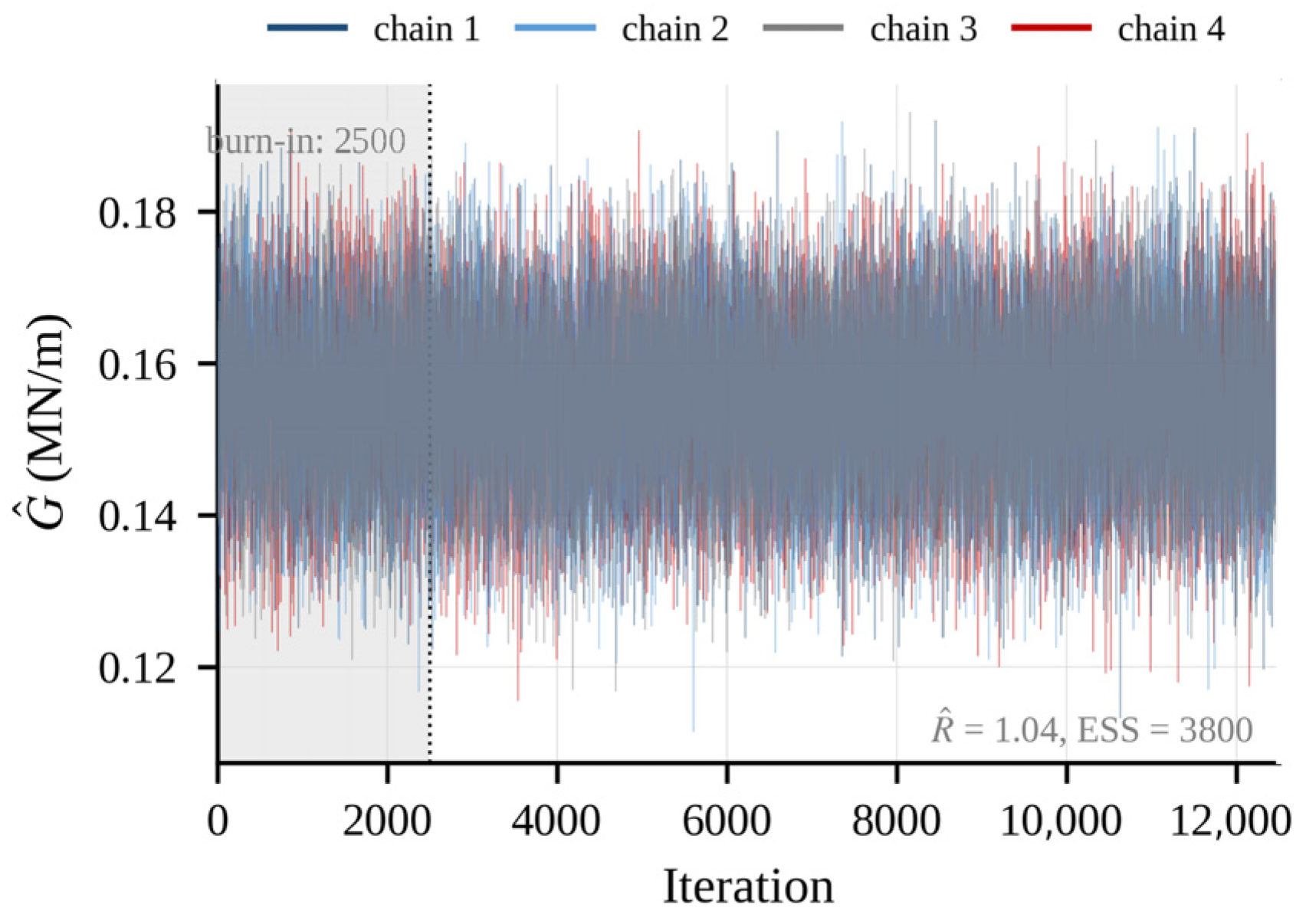
Figure A2.
MCMC traces for the noise nuisance parameter σf from four chains with burn-in shading ( = 1.02, ESS = 3900).
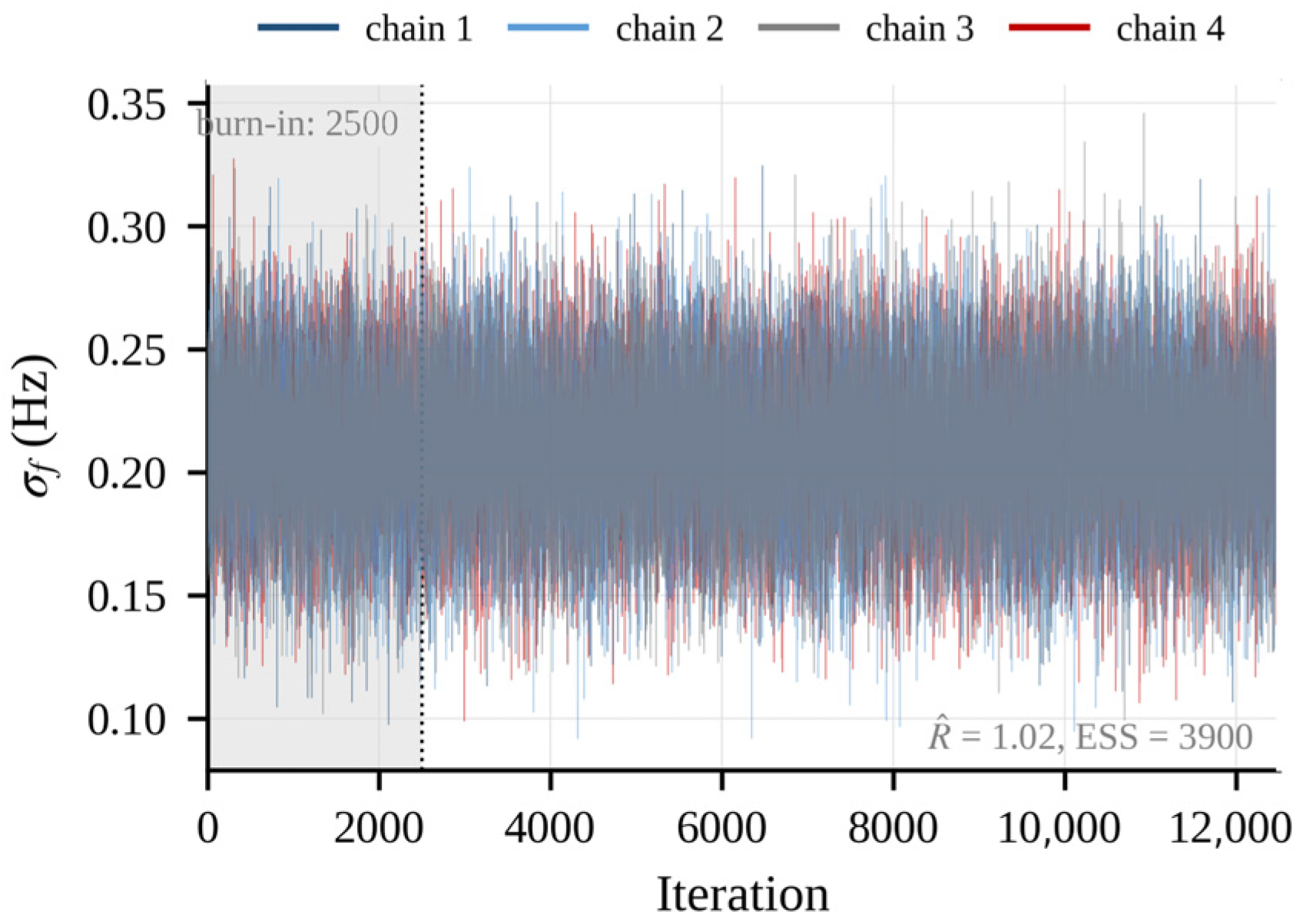
Figure A3.
Autocorrelation function of the thinned k draws for the four chains; dashed lines mark ±0.05.
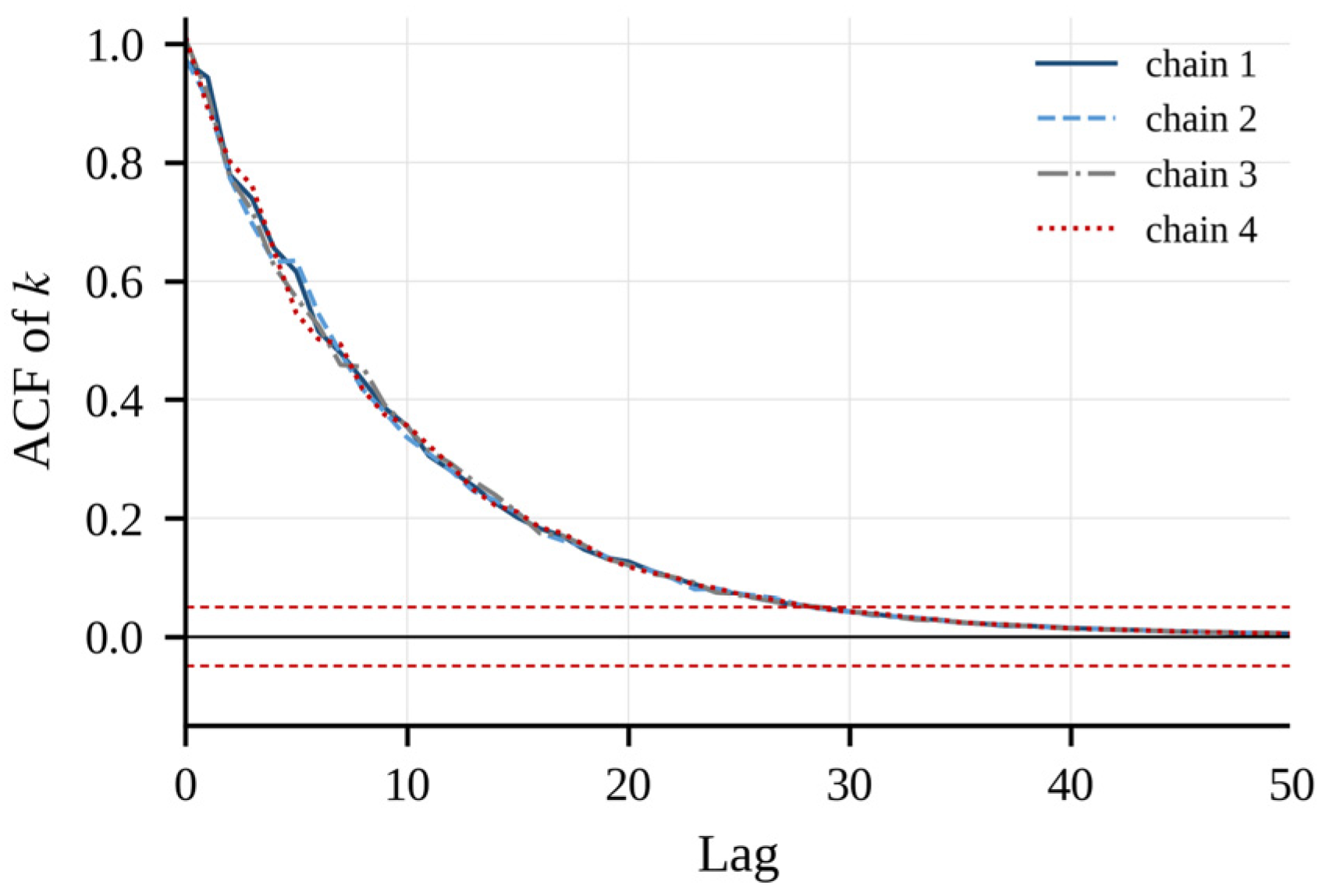
Figure A4.
Autocorrelation function of the thinned draws for the four chains; dashed lines mark ±0.05.
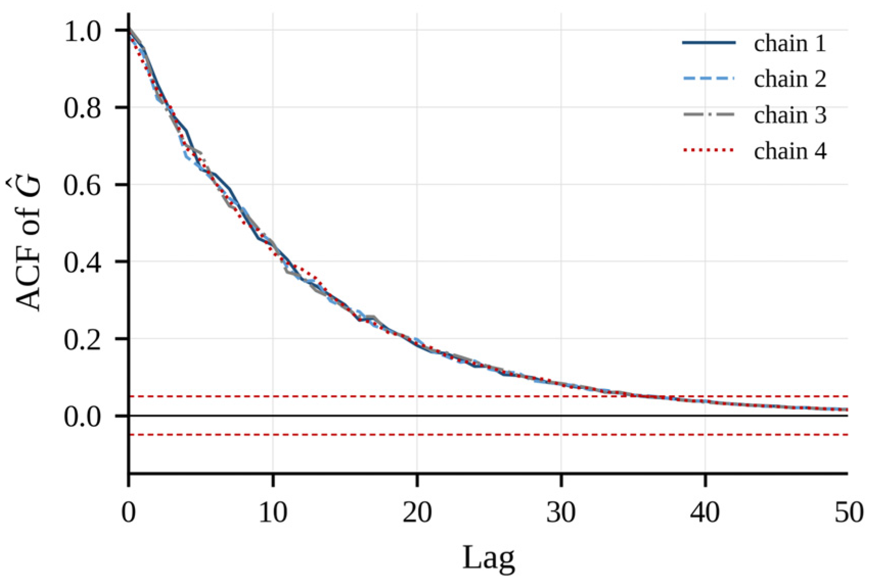
Figure A5.
Autocorrelation function of the thinned σf draws for the four chains; dashed lines mark ±0.05.
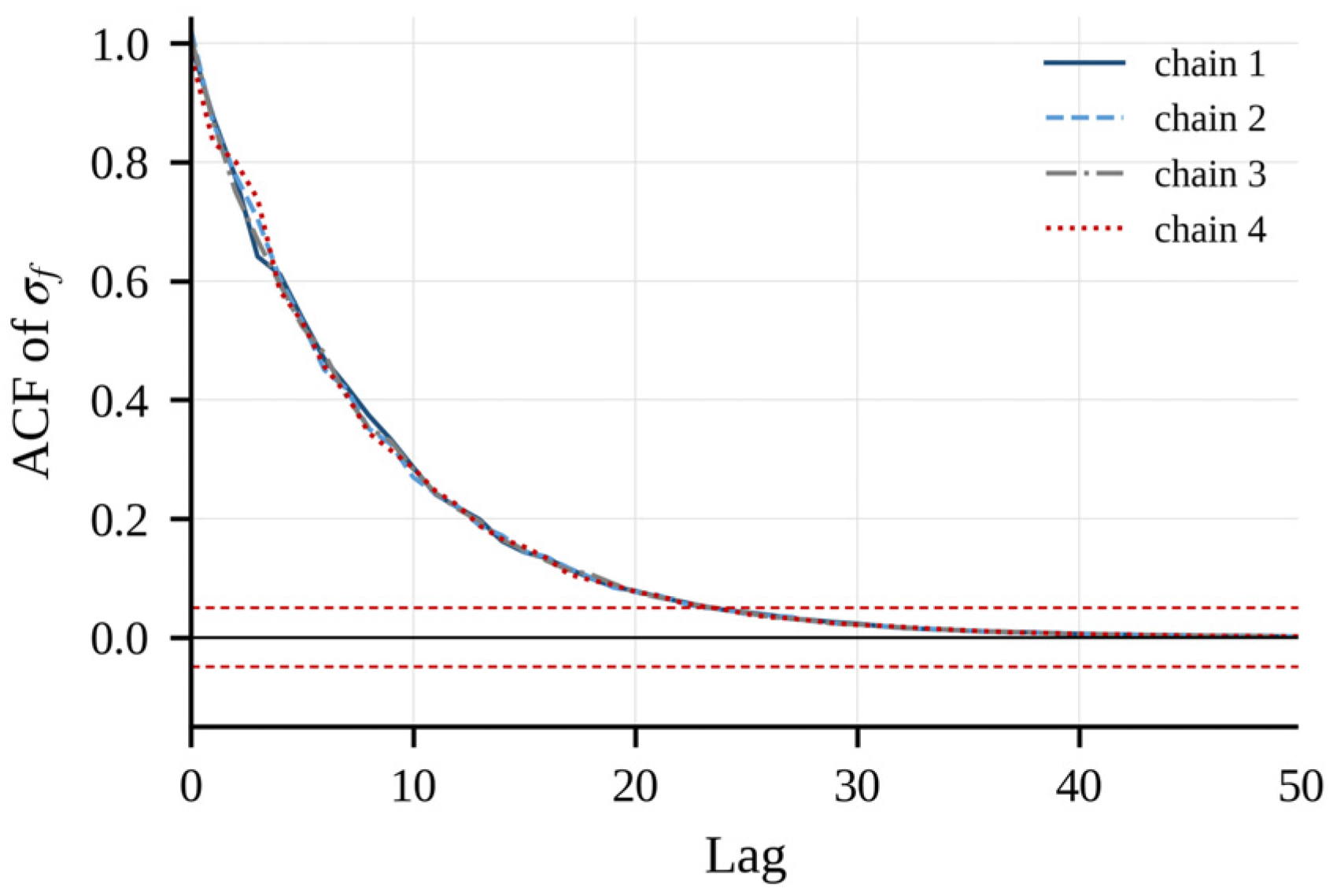
The posterior predictive check (Figure A6) compares the observed plate frequencies with the 95% posterior predictive intervals: all three observations fall inside their intervals, and the predictive medians track the observations to within the spectral resolution of Section 7.2, indicating adequate model fit without over-concentration.
Figure A6.
Posterior predictive check at the fundamental mode: observed fundamental frequencies (red diamonds) versus predictive medians (blue) and 95% posterior predictive intervals (gray bands) at f1: (a) plate B1; (b) plate B2; (c) plate B3. The likelihood contains only the fundamental frequency of each plate (three observations in total); because this paper derives no higher-mode forward model, the check is restricted to the fundamental mode and no higher-mode predictions are shown.
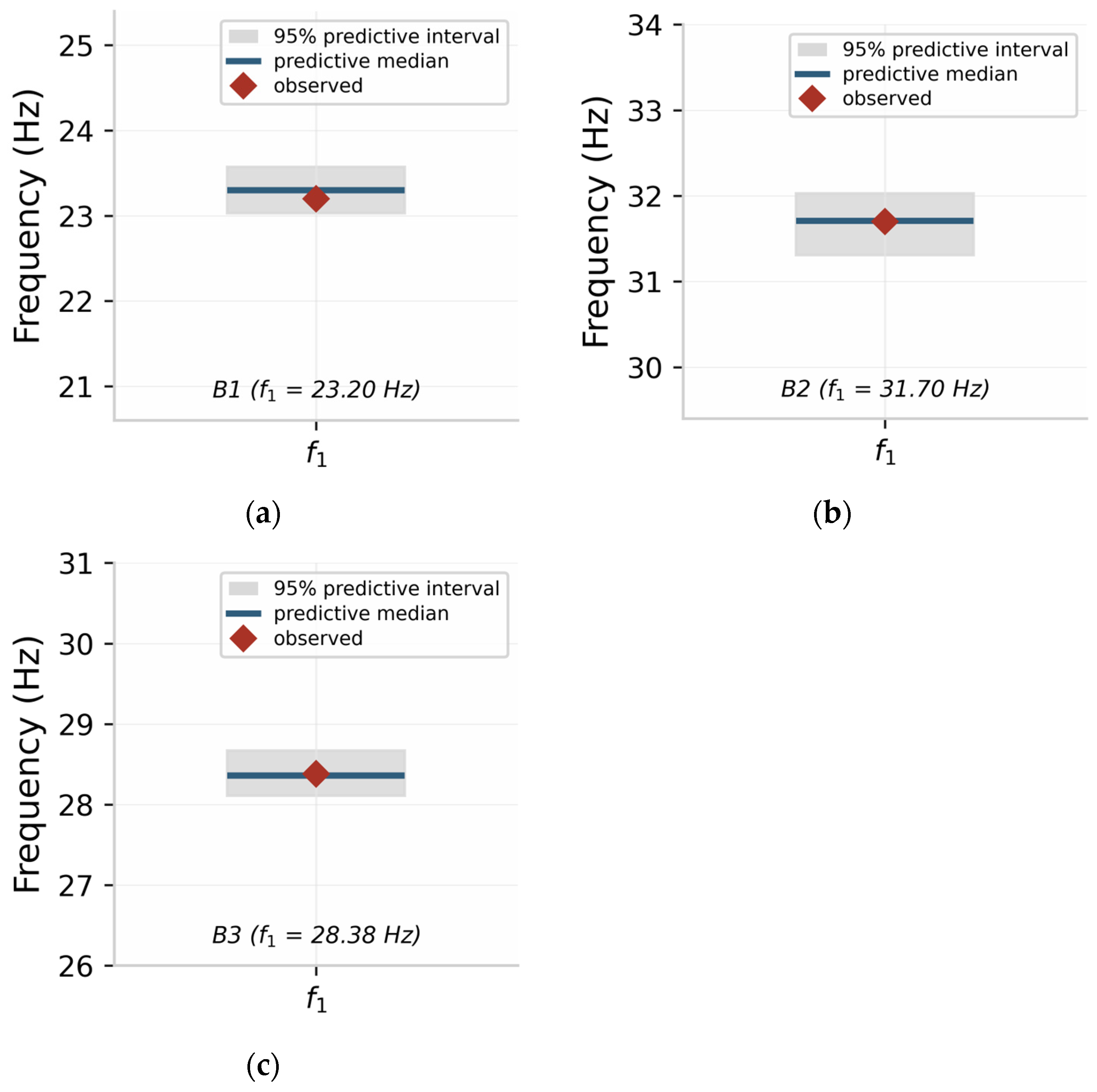
Prior sensitivity. The informative prior on k was halved (σ = 0.75 MPa/m) and doubled (σ = 3.0 MPa/m) about the base value (σ = 1.5 MPa/m), and the adaptive MCMC procedure of Section 5.1 was re-run with identical chains, burn-in and thinning (Table A4, produced by the same sampling chain as Section 5.2, with only the prior changed). The posterior mean of k shifts by at most 0.26 MPa/m (4.3%) across the four configurations and the posterior of is essentially unaffected (0.150–0.155 MN/m), confirming that the informative prior stabilizes but does not drive the identification. Replacing the informative prior with a fully uninformative uniform prior over the same truncation interval 1–20 MPa/m shifts the posterior mean of the compression coefficient by 0.15 MPa/m and leaves the shear layer stiffness essentially unchanged (Table A4, last row): the three-plate likelihood, though weak, already localizes the compression coefficient to within about ±0.6 MPa/m, and the K30 evidence acts as a stabilizer rather than the dominant information source.
Table A4.
Prior-sensitivity analysis of the posterior distributions (adaptive Metropolis–Hastings, 4 chains × 12,500 iterations, burn-in 2500, thinning 5; all rows from the same sampling chain as Section 5.2, with only the prior changed).
Figure A7.
Robustness of the identified parameters to frequency measurement noise: (a) relative error of k; (b) relative error of . Violin distributions summarize 500 Monte Carlo identifications per injected noise level (0.5–5% in steps of 0.5%), with least-squares fits and the Cramér–Rao trend of Equation (18) overlaid (the three coincide); fitted sensitivities are approximately 7.0% (k) and per 1% of frequency noise, reaching the 15% engineering acceptance limit at injected levels of about 2.1% (k) and .
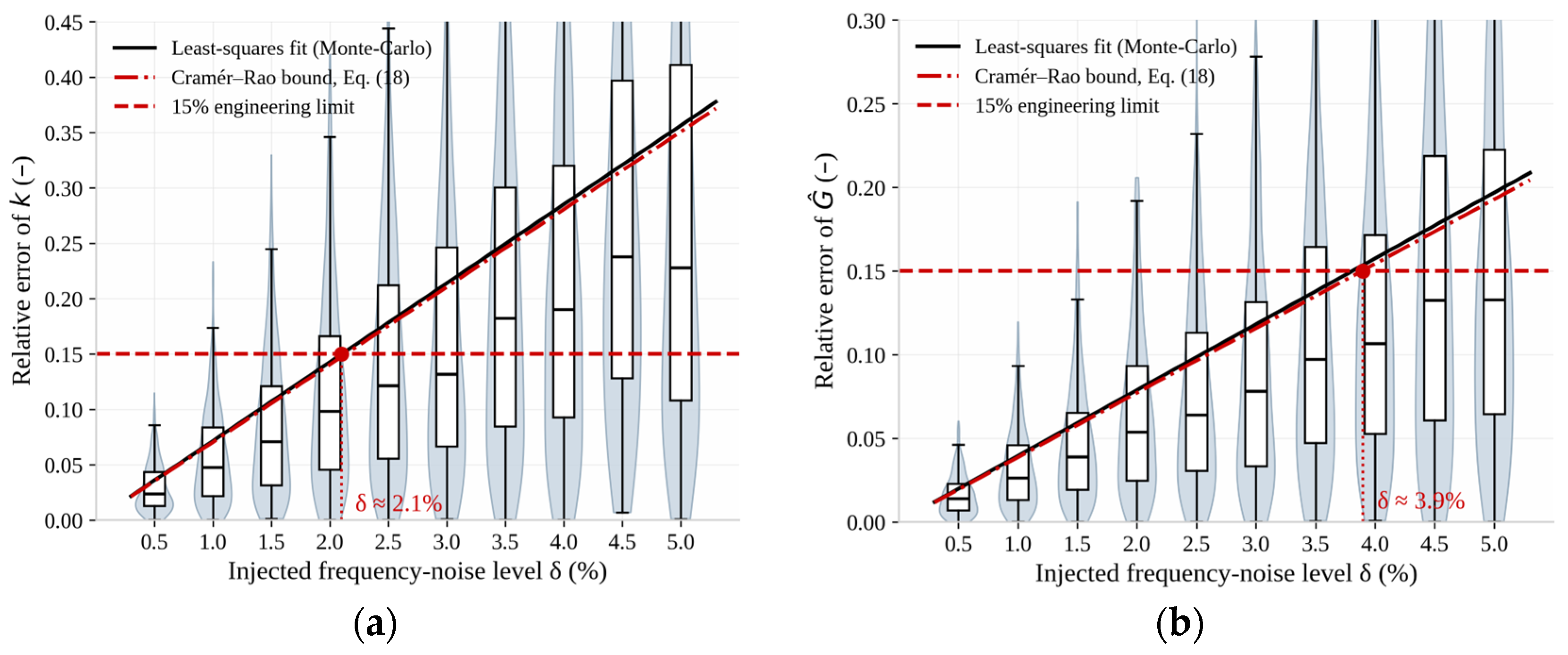
Appendix C. Finite-Element Model Setup
Table A5 gives the full input specification of the Abaqus 2026 consolidation model, built on the soil profile of Figure 2, together with the SAP2000 v27 modal model settings. The constitutive assignment follows Section 6.1: Modified cam-clay for the muddy silty clay (λ = 0.14, κ = 0.02, M = 1.27), Drucker–Prager for the silty clay layers, Duncan–Chang hyperbolic elasticity for the new fill (K = 150, n = 0.40, Rf = 0.85, Kb = 75, m = 0.5) and linear elasticity for the sand mat. The Duncan–Chang Rf, Kb and m values and the per-layer permeabilities are typical values adopted in the absence of site-specific tests; their influence on the 15-year responses is bounded by the Sobol analysis of Section 5.3, which shows that the responses of engineering interest are governed by the identified k and rather than by these secondary parameters.
Table A5.
Full input specification of the Abaqus 2026 and SAP2000 v27 models (soil profile of Figure 2).
Appendix D. Preliminary Carbon Estimate
Table A6 computes the per-site carbon saving of the accelerometer campaign relative to a conventional K30 static-testing campaign, following the boundary definitions of [13,14] and the Chinese national guideline for greenhouse gas accounting of land transportation enterprises [53] (diesel 2.64 kg CO2e/L from a net calorific value of 43.33 GJ/t, carbon content 20.2 tC/TJ, oxidation rate 98% and density 0.84 kg/L; gasoline 2.22 kg CO2e/L from 44.80 GJ/t, 18.9 tC/TJ, 98% and 0.73 kg/L; typical passenger car consumption 8.0 L/100 km). The estimate is preliminary and order-of-magnitude only: it assumes typical mobilization distances and traffic flows for a provincial expressway site, and it excludes the embodied emissions of the instruments—which are of comparable class and mass for the two methods and small beside the vehicle operations—as well as the negligible battery power of the accelerometers; it should be refined with project-specific logistics before any use in procurement. The detour component (about 75% of the total) is an attribution assumption based on the lane closure durations typical of K30 campaigns on operating expressways and is the least certain component of the estimate. A conservative scenario that halves the detour attribution still yields a saving of about 1.5 t CO2e per site, so the qualitative conclusion—that the accelerometer campaign avoids a substantial fraction of the testing-related emissions—does not depend on the detour assumption; the estimate is nevertheless reported as preliminary rather than as a life-cycle assessment.
Table A6.
Carbon comparison per site (assumption-transparent preliminary estimate).
Appendix E. Interface Patch Test
The shear link interface of Section 6.1 was verified by a patch test (Figure A8). A line load is applied to the discrete interface and the resulting settlement trough is compared with the analytical Pasternak solution for the same load and parameters. The maximum deviation over the trough at the final node spacing Δx = 0.125 m is 3.4%, within the 5% verification tolerance. As a control, a Winkler spring array of matched compression stiffness is subjected to the same load: it cannot reproduce the trough extent, demonstrating graphically that the ∇2w coupling exists only when the shear links are present. Mesh convergence is documented at Δx = 0.50, 0.25 and 0.125 m: between the two finest meshes (Δx = 0.25 m → 0.125 m) the 15-year differential settlement changes by 1.6% and the lateral displacement by 1.1%.
Figure A8.
Patch test of the discrete shear link interface under a line load: settlement trough of the analytical Pasternak solution (solid line), the discrete shear link solutions at node spacings Δx = 0.50, 0.25 and 0.125 m (markers), and the matched-stiffness Winkler control (cross); the maximum deviation over the trough at Δx = 0.125 m is 3.4%.
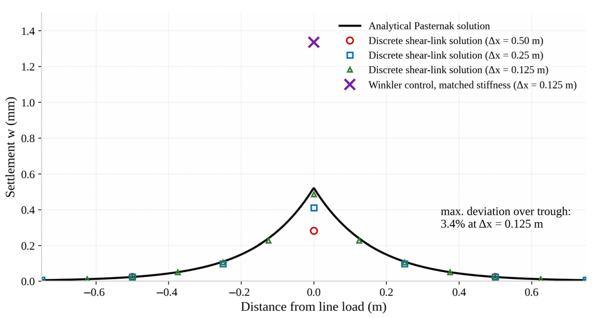
References
- Allersma, H.G.B.; Ravenswaay, L.; Vos, E. Investigation of road widening on soft soils using a small centrifuge. Transp. Res. Rec. 1994, 1462, 47–53. Available online: https://onlinepubs.trb.org/Onlinepubs/trr/1994/1462/1462-006.pdf (accessed on 16 September 2026).
- Lin, J.; Zhang, N.; Zhang, Y. Study of the prediction of vibrations in soft soil foundations based on field tests. Sensors 2024, 24, 2564. [Google Scholar] [CrossRef] [Scilit] [PubMed]
- Selvadurai, A.P.S. Elastic Analysis of Soil–Foundation Interaction; Elsevier: Amsterdam, The Netherlands, 1979. [Google Scholar]
- Younesian, D.; Hosseinkhani, A.; Askari, H.; Esmailzadeh, E. Elastic and viscoelastic foundations: A review on linear and nonlinear vibration modeling and applications. Nonlinear Dyn. 2019, 97, 853–895. [Google Scholar] [CrossRef] [Scilit]
- Winkler, E. Die Lehre von der Elastizität und Festigkeit; H. Dominicus: Prague, Czech Republic, 1867. [Google Scholar]
- Hetenyi, M. Beams on Elastic Foundation; University of Michigan Press: Ann Arbor, MI, USA, 1946. [Google Scholar]
- Kerr, A.D. Elastic and viscoelastic foundation models. J. Appl. Mech. 1964, 31, 491–498. [Google Scholar] [CrossRef] [Scilit]
- Yu, H.; Cai, C.; Yuan, Y.; Jia, M. Analytical solutions for Euler–Bernoulli beam on Pasternak foundation subjected to arbitrary dynamic loads. Int. J. Numer. Anal. Methods Geomech. 2017, 41, 1125–1137. [Google Scholar] [CrossRef] [Scilit]
- Vlasov, V.Z.; Leontiev, U.N. Beams, Plates and Shells on Elastic Foundations; Israel Program for Scientific Translations: Jerusalem, Israel, 1966. [Google Scholar]
- Terzaghi, K. Evaluation of coefficients of subgrade reaction. Géotechnique 1955, 5, 297–326. [Google Scholar] [CrossRef] [Scilit]
- Yao, Y.; Ma, Z.S.; Ding, Q.; Han, J.; Sui, X.; Liu, B. Stiffness identification of beam structures with elastic foundations through the global mode method and time-domain nonlinear subspace method. Nonlinear Dyn. 2025, 113, 4447–4464. [Google Scholar] [CrossRef] [Scilit]
- Han, J. Principles and Practice of Ground Improvement; John Wiley & Sons: Hoboken, NJ, USA, 2015. [Google Scholar]
- Shillaber, C.M.; Mitchell, J.K.; Dove, J.E. Energy and carbon assessment of ground improvement works. I: Definitions and background. J. Geotech. Geoenviron. Eng. 2016, 142, 04015083. [Google Scholar] [CrossRef] [Scilit]
- Shillaber, C.M.; Mitchell, J.K.; Dove, J.E. Energy and carbon assessment of ground improvement works. II: Working model and example. J. Geotech. Geoenviron. Eng. 2016, 142, 04015084. [Google Scholar] [CrossRef] [Scilit]
- Shahsavari, D.; Shahsavari, M.; Li, L.; Karami, B. A novel quasi-3D hyperbolic theory for free vibration of FG plates with porosities resting on Winkler/Pasternak/Kerr foundation. Aerosp. Sci. Technol. 2018, 72, 134–149. [Google Scholar] [CrossRef] [Scilit]
- Zhang, H.; Shi, D.Y.; Wang, Q.S. Free vibration analysis of the moderately thick laminated composite rectangular plate on two-parameter elastic foundation with elastic boundary conditions. KnE Mater. Sci. 2016, 1, 190–193. [Google Scholar] [CrossRef] [Scilit]
- Celep, Z.; Özcan, Z.; Güner, A. Elastic triangular plate dynamics on unilateral Winkler foundation: Analysis using Chebyshev polynomial expansion for forced vibrations. J. Mech. Sci. Technol. 2025, 39, 65–79. [Google Scholar] [CrossRef] [Scilit]
- Kurpa, L.; Pellicano, F.; Shmatko, T.; Zippo, A. Free vibration analysis of porous functionally graded material plates with variable thickness on an elastic foundation using the R-functions method. Math. Comput. Appl. 2024, 29, 10. [Google Scholar] [CrossRef] [Scilit]
- Shirzad-Ghaleroudkhani, N.; Mahsuli, M.; Ghahari, S.F.; Taciroglu, E. Bayesian identification of soil–foundation stiffness of building structures. Struct. Control Health Monit. 2018, 25, e2090. [Google Scholar] [CrossRef] [Scilit]
- Huang, Y.; Beck, J.L.; Li, H. Bayesian system identification based on hierarchical sparse Bayesian learning and Gibbs sampling with application to structural damage assessment. Comput. Methods Appl. Mech. Eng. 2017, 318, 382–411. [Google Scholar] [CrossRef] [Scilit]
- Li, B.; Der Kiureghian, A.; Au, S.K. A Gibbs sampling algorithm for structural modal identification under seismic excitation. Earthq. Eng. Struct. Dyn. 2018, 47, 2735–2755. [Google Scholar] [CrossRef] [Scilit]
- Gumus, O.; Gonen, S.; Pela, L.; Roca Fabregat, P.; Erduran, E. Probabilistic Bayesian model updating of two laboratory-scale structures using ambient vibration measurements. In Proceedings of the 12th European Workshop on Structural Health Monitoring (EWSHM 2026), Toulouse, France, 7–10 July 2026. [Google Scholar] [CrossRef] [Scilit] [PubMed]
- Zhang, J.; Zhou, C.W.; Jia, C.; Lin, J. Powell inversion mechanical model of foundation parameters with generalized Bayesian theory. J. Zhejiang Univ.-Sci. A 2017, 18, 567–578. [Google Scholar] [CrossRef] [Scilit]
- Sheil, B.; Anagnostopoulos, C.; Buckley, R.; Ciantia, M.O.; Febrianto, E.; Fu, J.; Gao, Z.; Geng, X.; Gong, B.; Hanley, K.; et al. Artificial intelligence transformations in geotechnics: Progress, challenges and future enablers. Comput. Geotech. 2026, 189, 107604. [Google Scholar] [CrossRef] [Scilit]
- Karniadakis, G.E.; Kevrekidis, I.G.; Lu, L.; Perdikaris, P.; Wang, S.; Yang, L. Physics-informed machine learning. Nat. Rev. Phys. 2021, 3, 422–440. [Google Scholar] [CrossRef] [Scilit]
- Raissi, M.; Perdikaris, P.; Karniadakis, G.E. Physics-informed neural networks: A deep learning framework for solving forward and inverse problems involving nonlinear partial differential equations. J. Comput. Phys. 2019, 378, 686–707. [Google Scholar] [CrossRef] [Scilit]
- Su, M.M.; Yu, Y.; Chen, T.H.; Guo, N.; Yang, Z.X. A thermodynamics-informed neural network for elastoplastic constitutive modeling of granular materials. Comput. Methods Appl. Mech. Eng. 2024, 430, 117246. [Google Scholar] [CrossRef] [Scilit]
- Yuan, B.; Choo, C.S.; Yeo, L.Y.; Wang, Y.; Yang, Z.; Guan, Q.; Suryasentana, S.; Choo, J.; Shen, H.; Megia, M.; et al. Physics-informed machine learning in geotechnical engineering: A direction paper. Geomech. Geoeng. 2025, 20, 1128–1159. [Google Scholar] [CrossRef] [Scilit]
- Zhang, P.; Yin, Z.Y.; Sheil, B. Interpretable data-driven constitutive modelling of soils with sparse data. Comput. Geotech. 2023, 160, 105511. [Google Scholar] [CrossRef] [Scilit]
- Zhang, P.; Yin, Z.Y.; Jin, Y.F. State-of-the-art review of machine learning applications in constitutive modeling of soils. Arch. Comput. Methods Eng. 2021, 28, 3661–3686. [Google Scholar] [CrossRef] [Scilit]
- Suh, H.S.; Song, J.Y.; Kim, Y.; Yu, X.; Choo, J. Data-driven discovery of interpretable water retention models for deformable porous media. Acta Geotech. 2024, 19, 3821–3835. [Google Scholar] [CrossRef] [Scilit]
- Zhang, L.; Guo, J.; Fu, X.; Tiong, R.L.K.; Zhang, P. Digital twin enabled real-time advanced control of TBM operation using deep learning methods. Autom. Constr. 2024, 158, 105240. [Google Scholar] [CrossRef] [Scilit]
- Sun, Z.; Li, H.; Bao, Y.; Meng, X.; Zhang, D. Intelligent risk prognosis and control of foundation pit excavation based on digital twin. Buildings 2023, 13, 247. [Google Scholar] [CrossRef] [Scilit]
- Pan, P.; Sun, S.H.; Feng, J.X.; Wen, J.T.; Lin, J.R.; Wang, H.S. Intelligent monitoring system for deep foundation pit based on digital twin. Buildings 2025, 15, 366. [Google Scholar] [CrossRef] [Scilit]
- Yu, C.; Liu, Z.; Wang, H.; Shi, G.; Song, T. Intelligent analysis of construction safety of large underground space based on digital twin. Buildings 2024, 14, 1551. [Google Scholar] [CrossRef] [Scilit]
- Versteijlen, W.G.; Renting, F.W.; Van Der Valk, P.L.C.; Bongers, J.; Van Dalen, K.N.; Metrikine, A.V. Effective soil-stiffness validation: Shaker excitation of an in-situ monopile foundation. Soil Dyn. Earthq. Eng. 2017, 102, 241–262. [Google Scholar] [CrossRef] [Scilit]
- Carbonari, S.; Dezi, F.; Arezzo, D.; Gara, F. A methodology for the identification of physical parameters of soil–foundation–bridge pier systems from identified state-space models. Eng. Struct. 2022, 255, 113944. [Google Scholar] [CrossRef] [Scilit]
- Davis, N.T.; Sanayei, M. Foundation identification using dynamic strain and acceleration measurements. Eng. Struct. 2020, 208, 109811. [Google Scholar] [CrossRef] [Scilit]
- Booshehrian, A.; Khazanovich, L. Dynamic analyses of a viscoelastic plate on a generalised Pasternak foundation. Int. J. Geotech. Eng. 2019, 13, 385–397. [Google Scholar] [CrossRef] [Scilit]
- Gazetas, G. Formulas and charts for impedances of surface and embedded foundations. J. Geotech. Eng. 1991, 117, 1363–1381. [Google Scholar] [CrossRef] [Scilit]
- Huynh, T.C.; Lee, S.Y.; Dang, N.L.; Kim, J.T. Vibration-based structural identification of caisson–foundation system via in situ measurement and simplified model. Struct. Control Health Monit. 2019, 26, e2315. [Google Scholar] [CrossRef] [Scilit]
- Hou, R.; Xia, Y. Review on the new development of vibration-based damage identification for civil engineering structures: 2010–2019. J. Sound Vib. 2021, 491, 115741. [Google Scholar] [CrossRef] [Scilit]
- Haario, H.; Saksman, E.; Tamminen, J. An adaptive Metropolis algorithm. Bernoulli 2001, 7, 223–242. [Google Scholar] [CrossRef] [Scilit]
- Gelman, A.; Rubin, D.B. Inference from iterative simulation using multiple sequences. Stat. Sci. 1992, 7, 457–472. [Google Scholar] [CrossRef] [Scilit]
- Saltelli, A.; Annoni, P.; Azzini, I.; Campolongo, F.; Ratto, M.; Tarantola, S. Variance based sensitivity analysis of model output. Design and estimator for the total sensitivity index. Comput. Phys. Commun. 2010, 181, 259–270. [Google Scholar] [CrossRef] [Scilit]
- Bland, J.M.; Altman, D.G. Measuring agreement in method comparison studies. Stat. Methods Med. Res. 1999, 8, 135–160. [Google Scholar] [CrossRef] [Scilit] [PubMed]
- Welch, P.D. The use of fast Fourier transform for the estimation of power spectra: A method based on time averaging over short, modified periodograms. IEEE Trans. Audio Electroacoust. 1967, 15, 70–73. [Google Scholar] [CrossRef] [Scilit]
- Peng, D. Evaluation Method of Foundation Coefficient of Two-Parameter Foundation Based on Dynamic Characteristic Test. Master’s Thesis, Hunan University, Changsha, China, 2017. (In Chinese) [Google Scholar]
- Peng, D. Finite element analysis of deformation characteristics of unilateral widening of expressway on soft soil foundation. Hunan Commun. Sci. Technol. 2019, 45, 55–58+139. (In Chinese) [Google Scholar]
- Dassault Systèmes SIMULIA. Abaqus 2026 Documentation (SIMULIA 2026 Release); Dassault Systèmes: Providence, RI, USA, 2025; Available online: https://help.3ds.com (accessed on 10 August 2026).
- Computers and Structures, Inc. SAP2000, v27.0.0; Release Notes (released 31 January 2026); Computers and Structures, Inc.: Walnut Creek, CA, USA, 2026. Available online: https://www.csiamerica.com/software/SAP2000/27/ReleaseNotesSAP2000v2700.pdf (accessed on 10 August 2026).
- Computers and Structures, Inc. SAP2000, v27.1.0; Release Notes (released 19 March 2026; adds the Faria concrete damage-plasticity model); Computers and Structures, Inc.: Walnut Creek, CA, USA, 2026. Available online: https://www.csiamerica.com/software/SAP2000/27/ReleaseNotesSAP2000v2710.pdf (accessed on 10 August 2026).
- National Development and Reform Commission of China. Guidelines for Greenhouse Gas Emission Accounting and Reporting for Land Transportation Enterprises (Trial); National Development and Reform Commission: Beijing, China, 2015. Available online: https://www.ndrc.gov.cn/xxgk/zcfb/tz/201511/W020190905506438255108.pdf (accessed on 16 August 2026). (In Chinese)
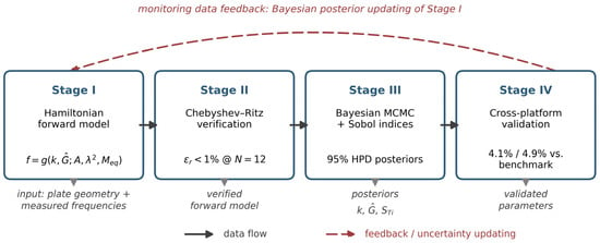
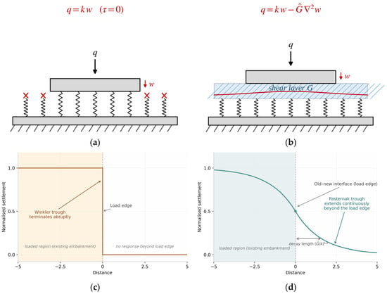
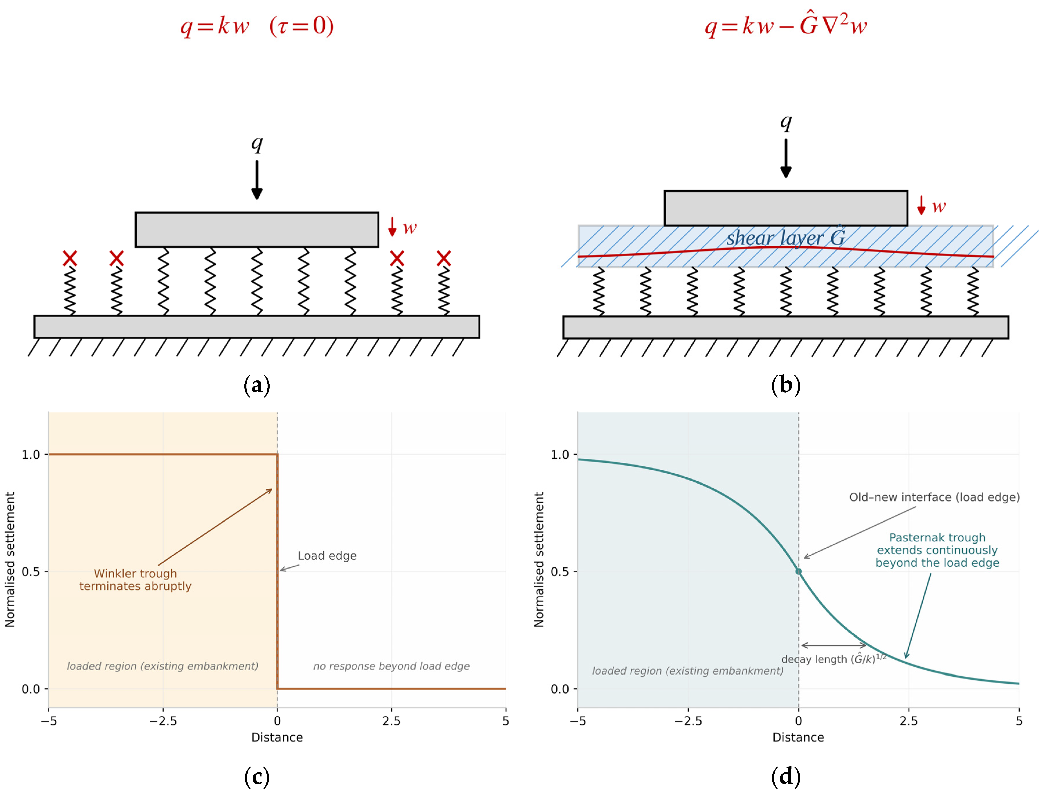
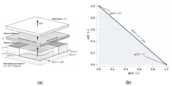
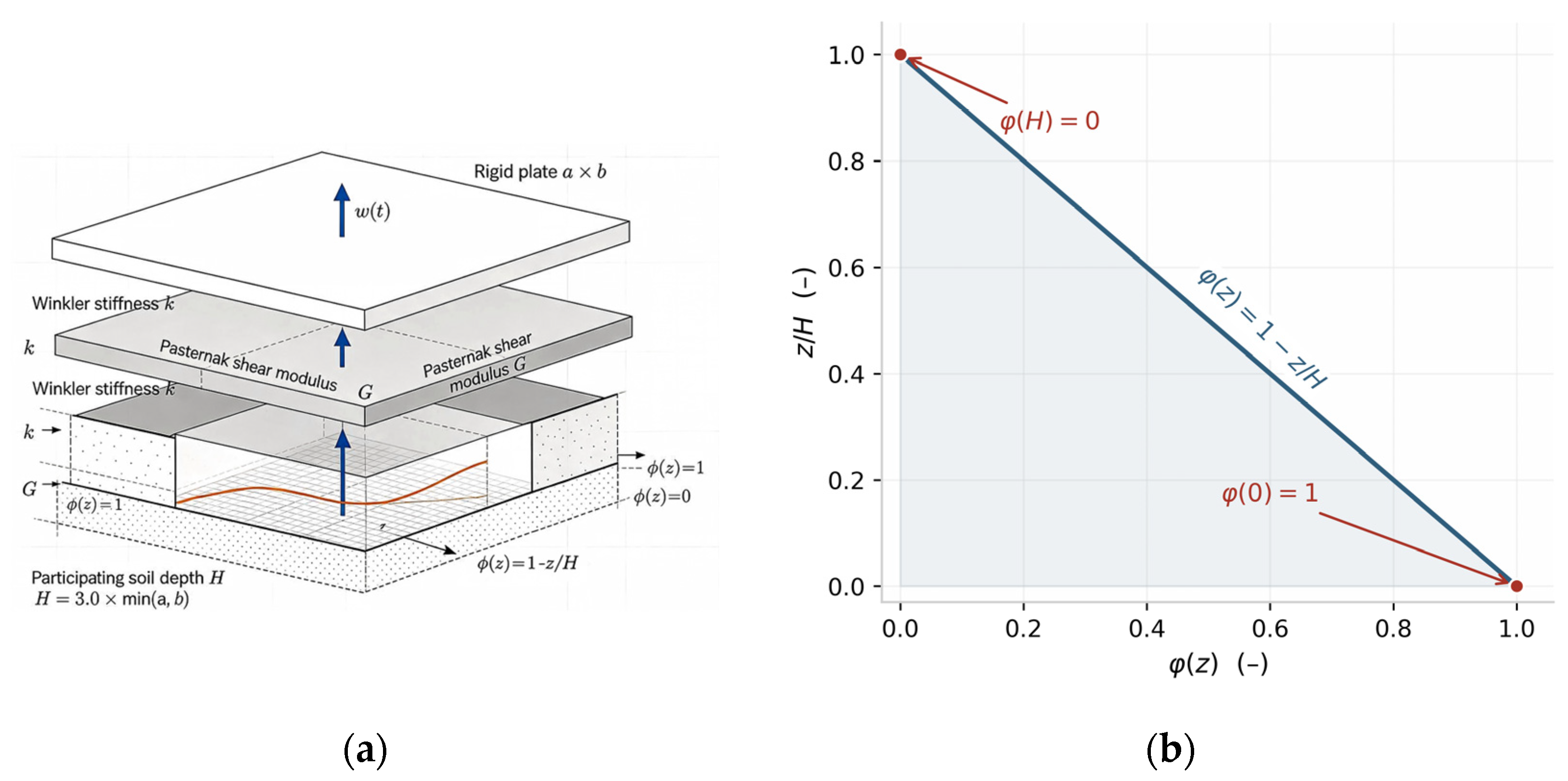
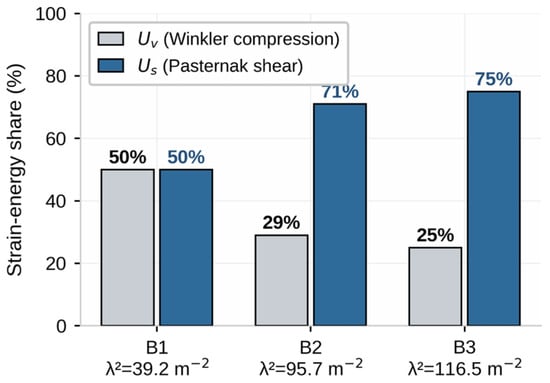
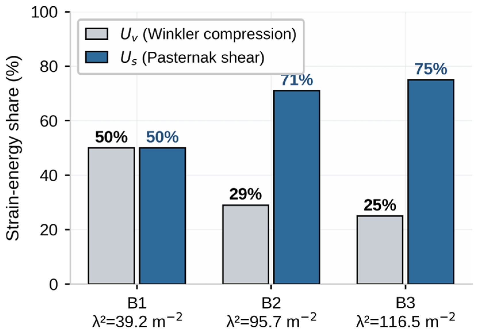
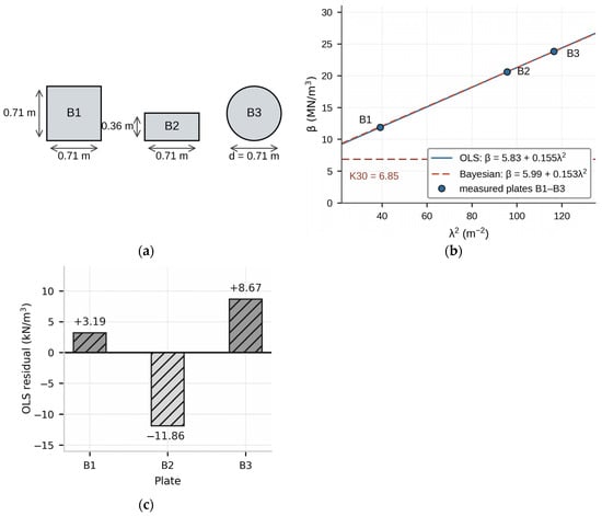
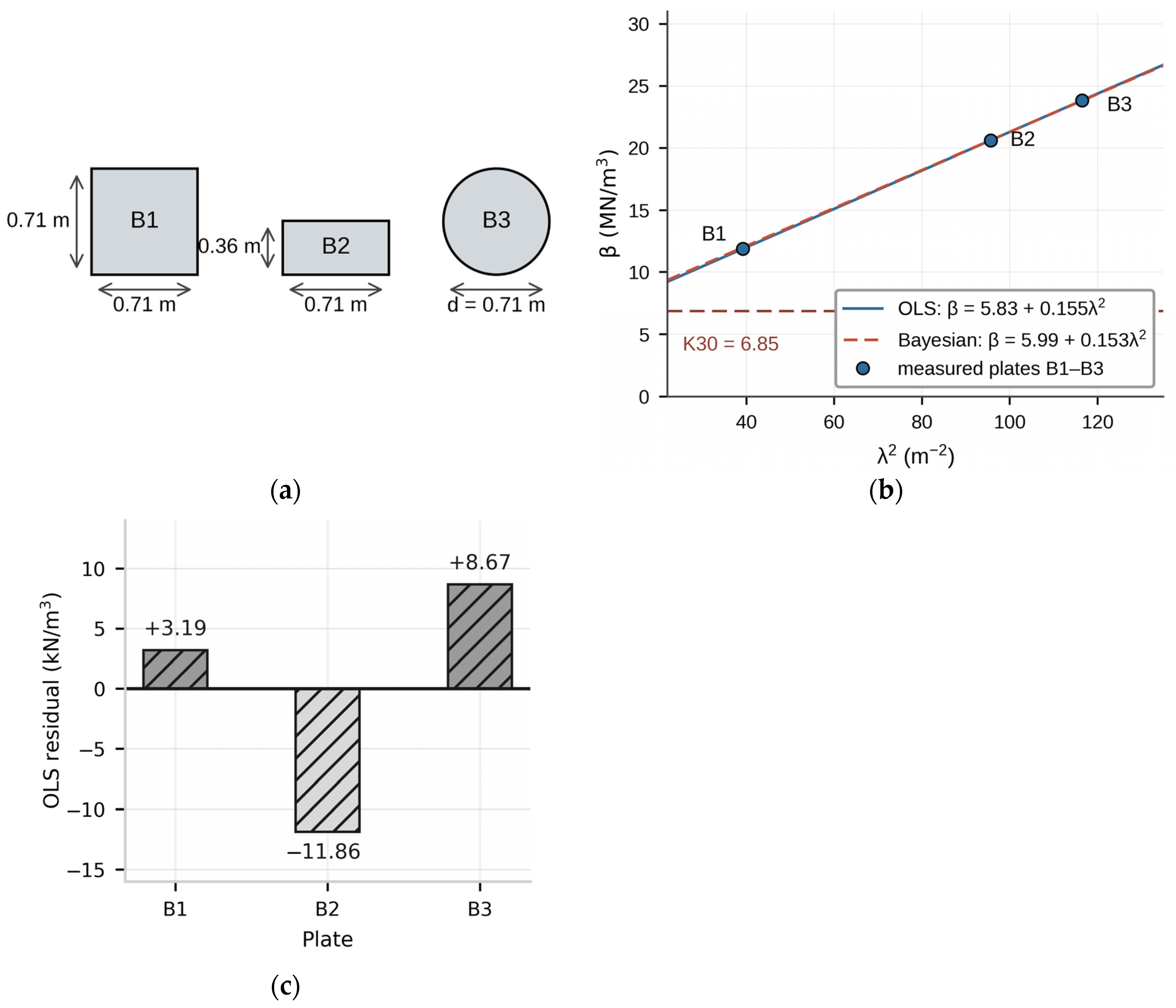
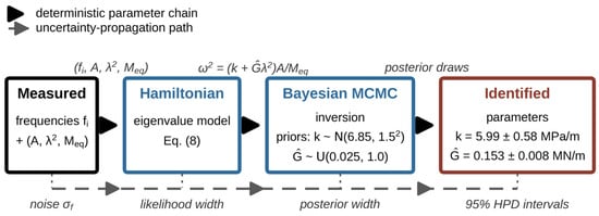
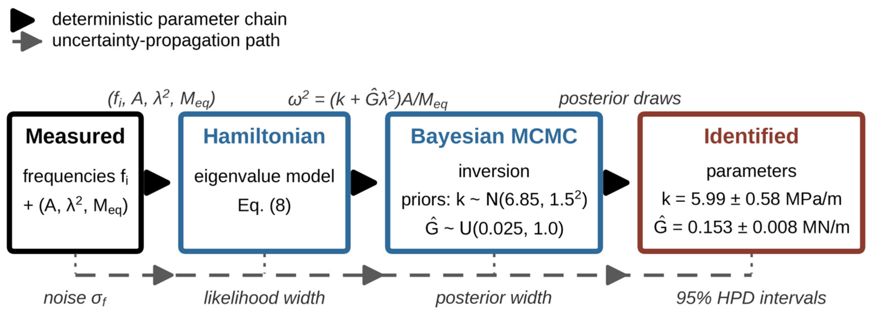
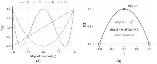
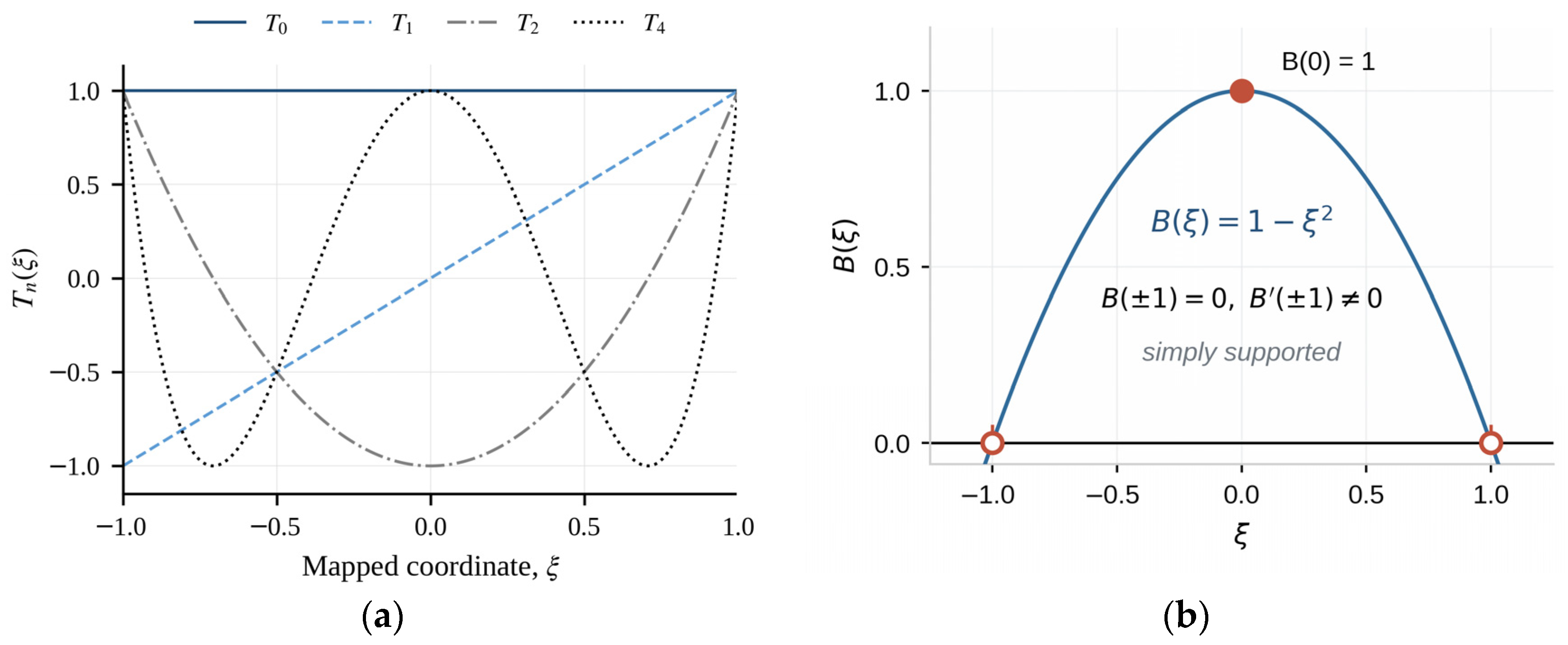
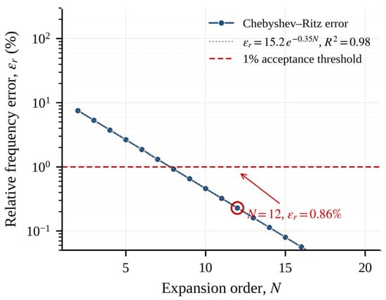
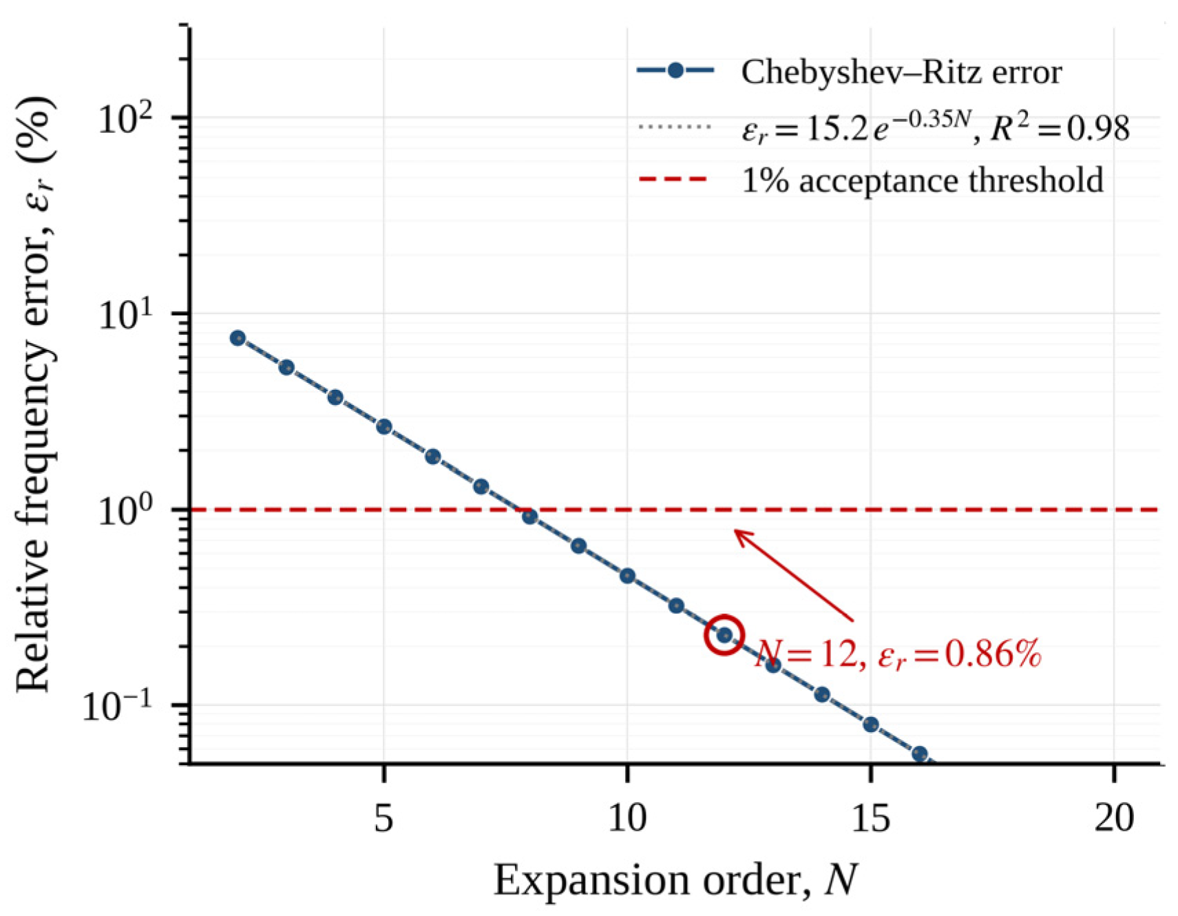
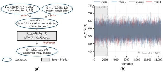
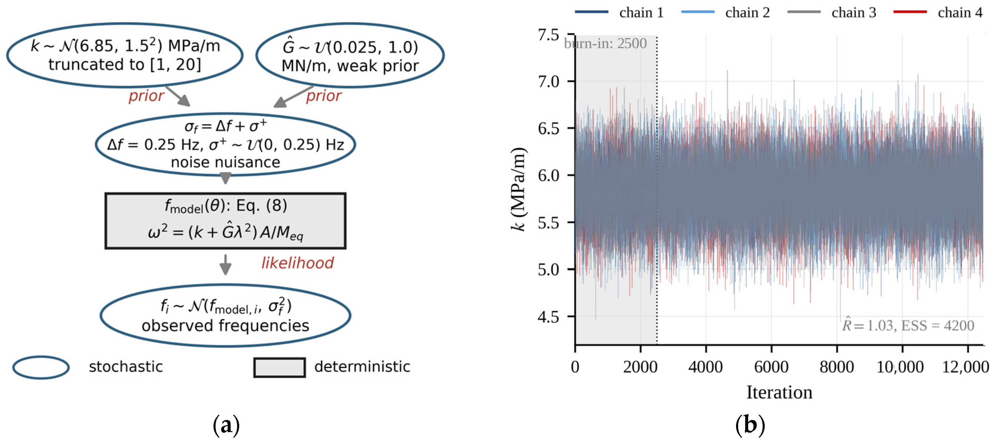
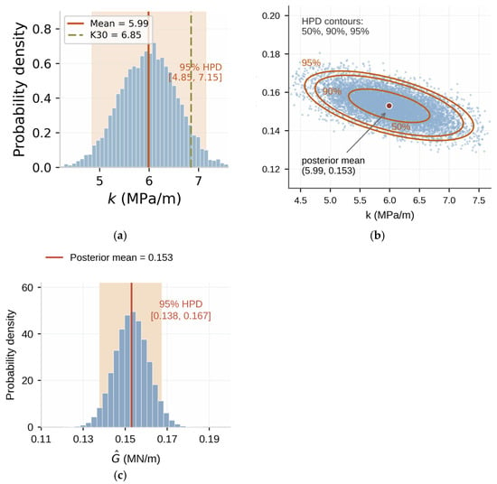
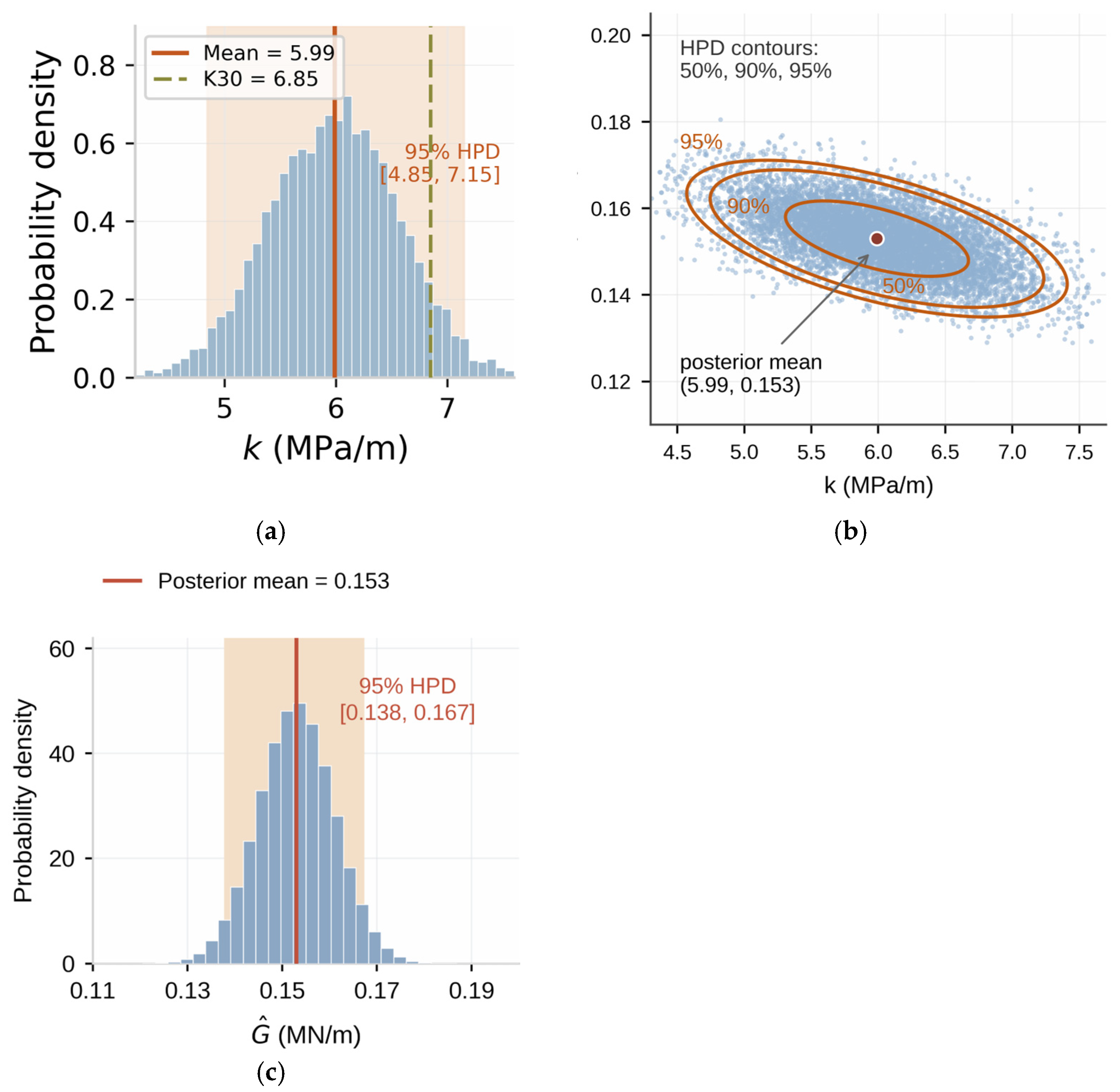
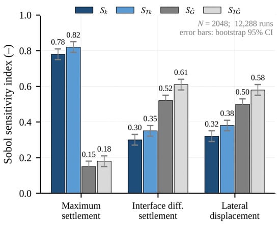
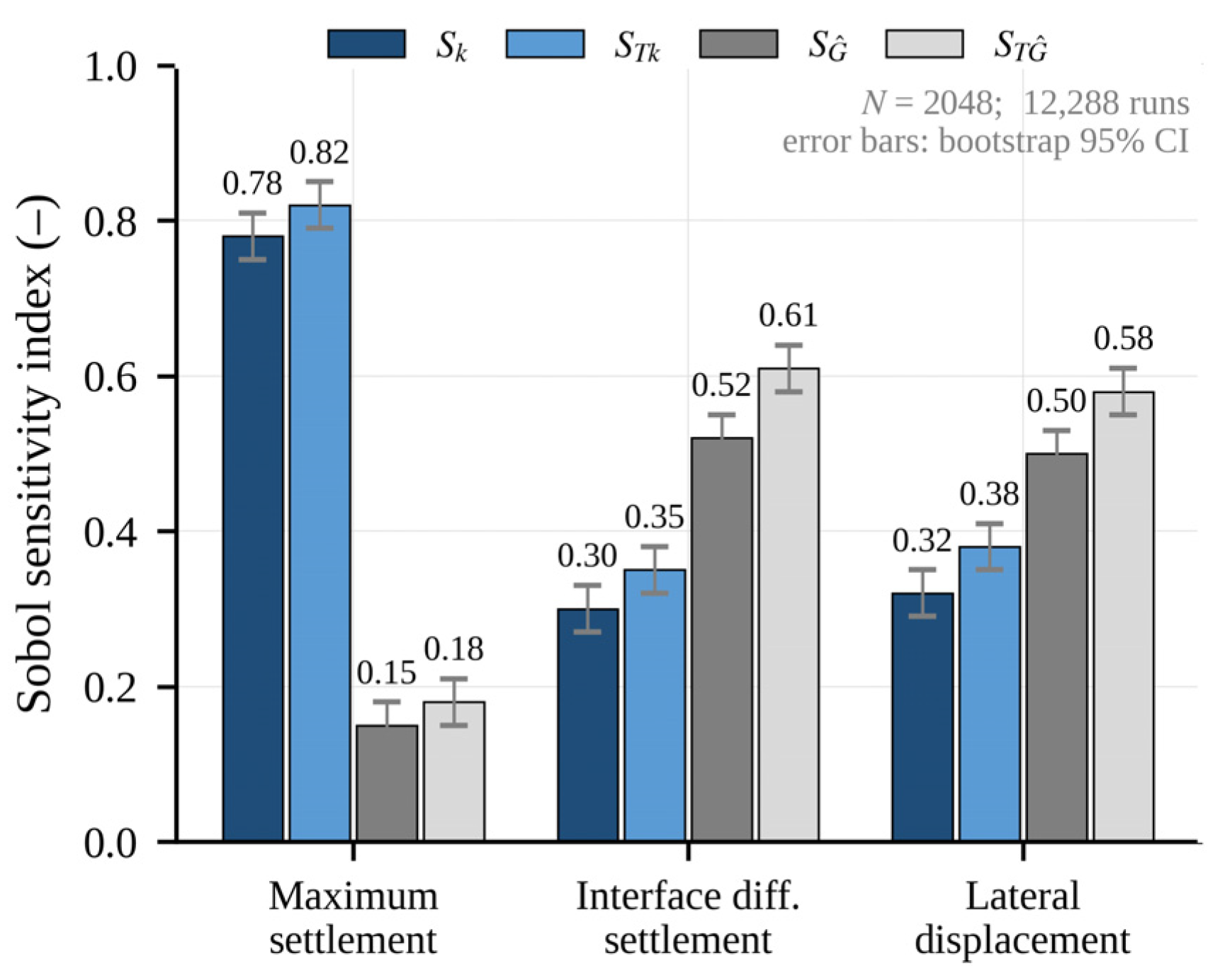
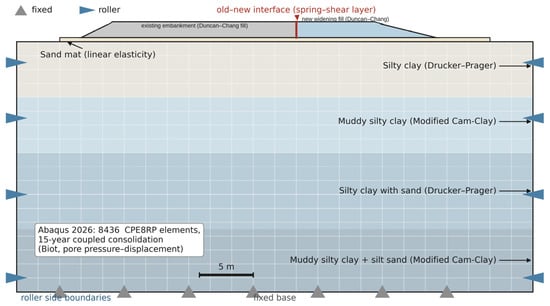
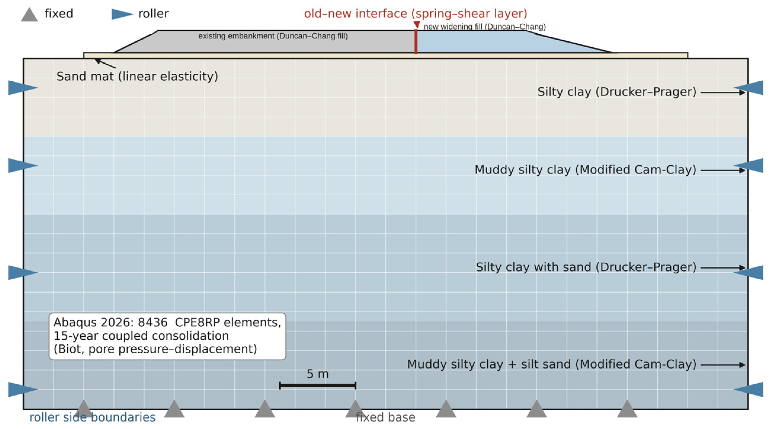
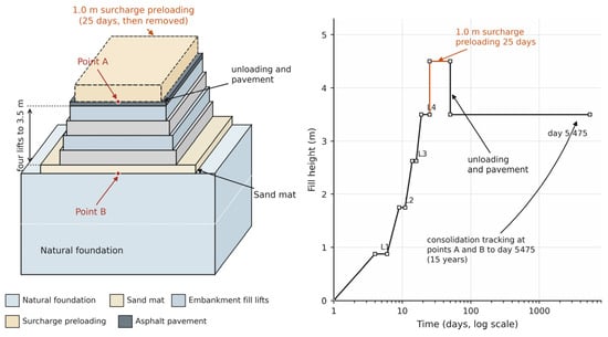
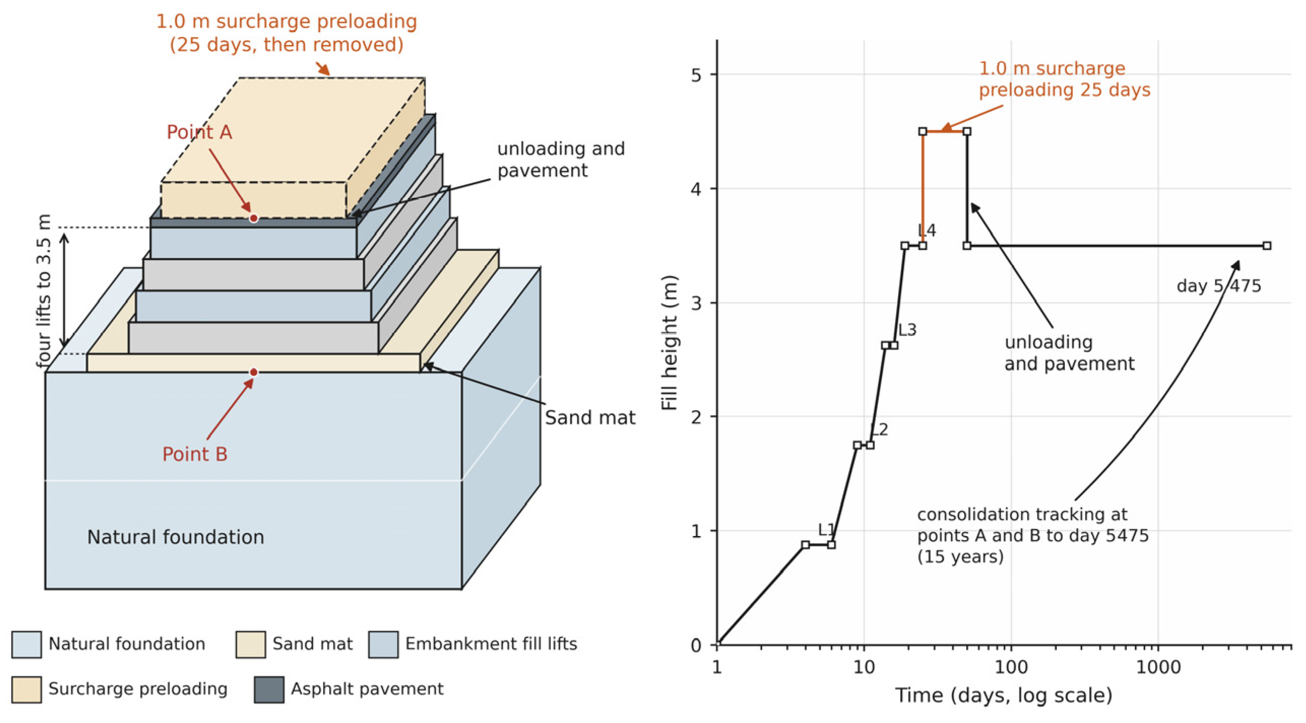
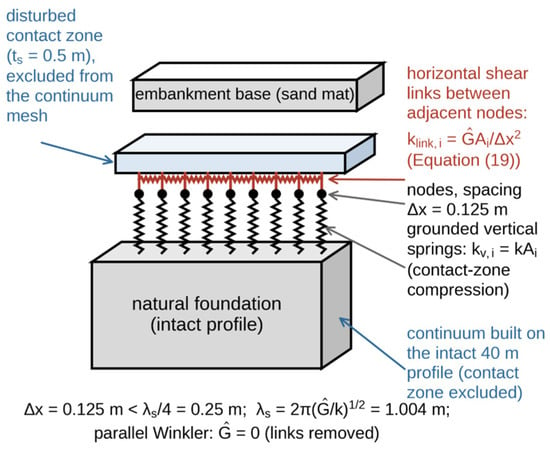
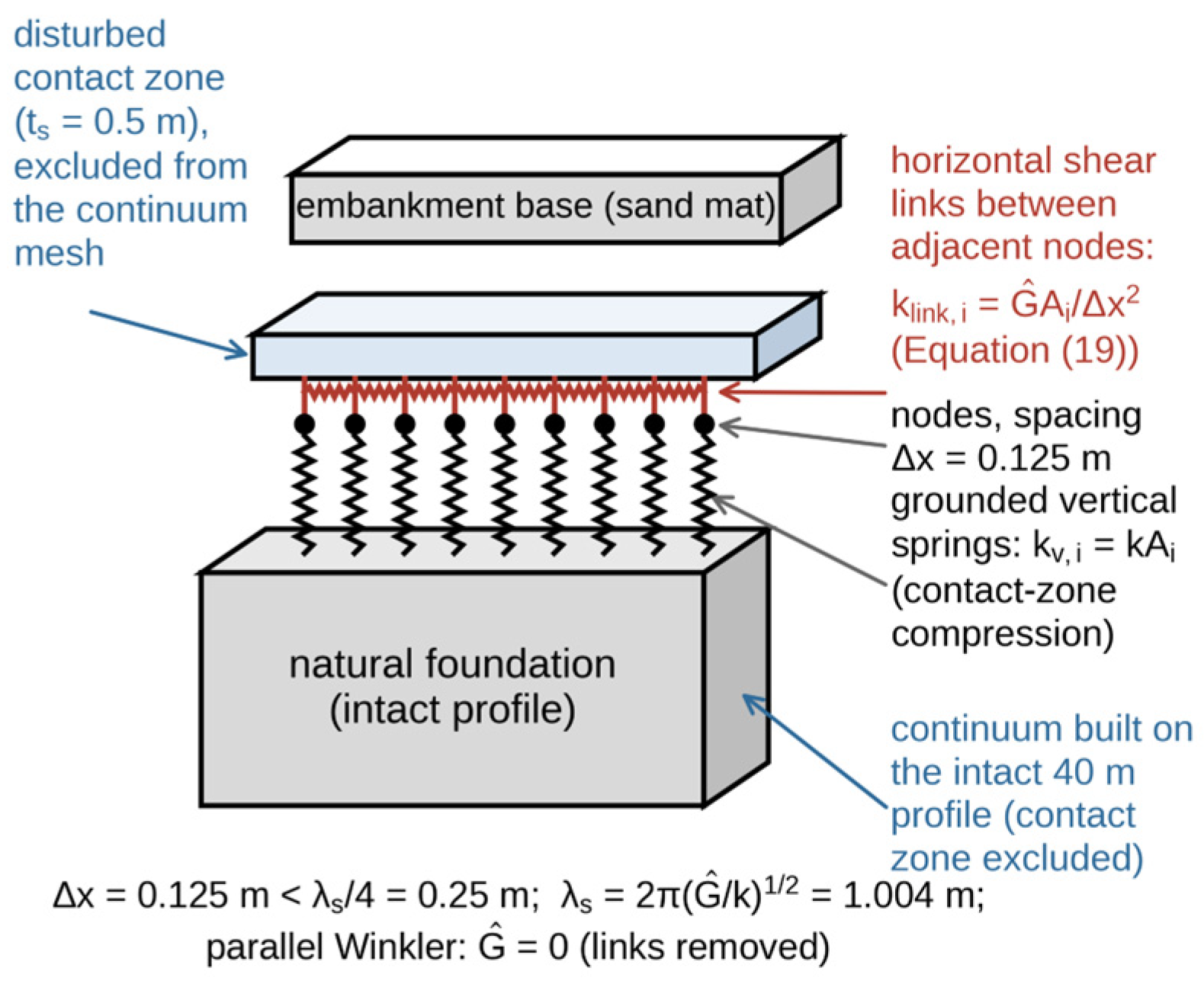
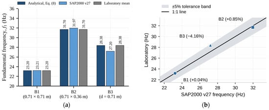
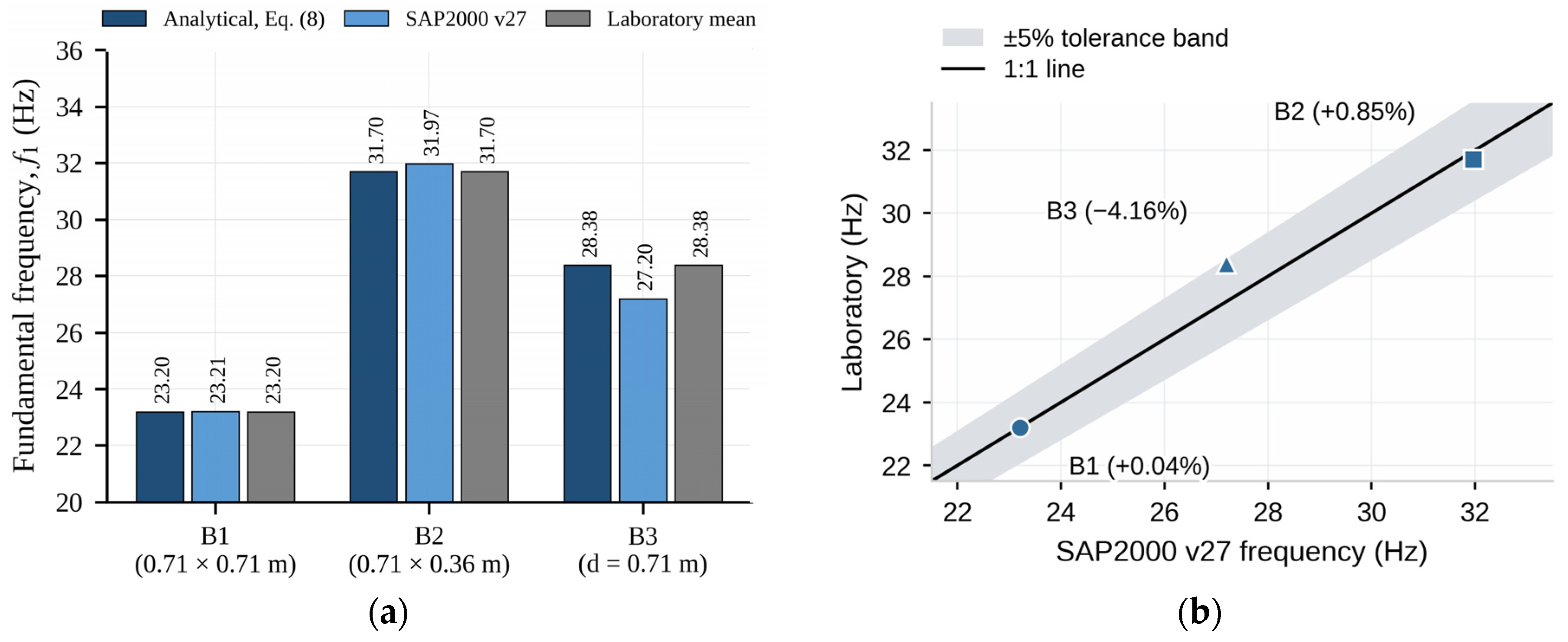
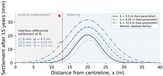
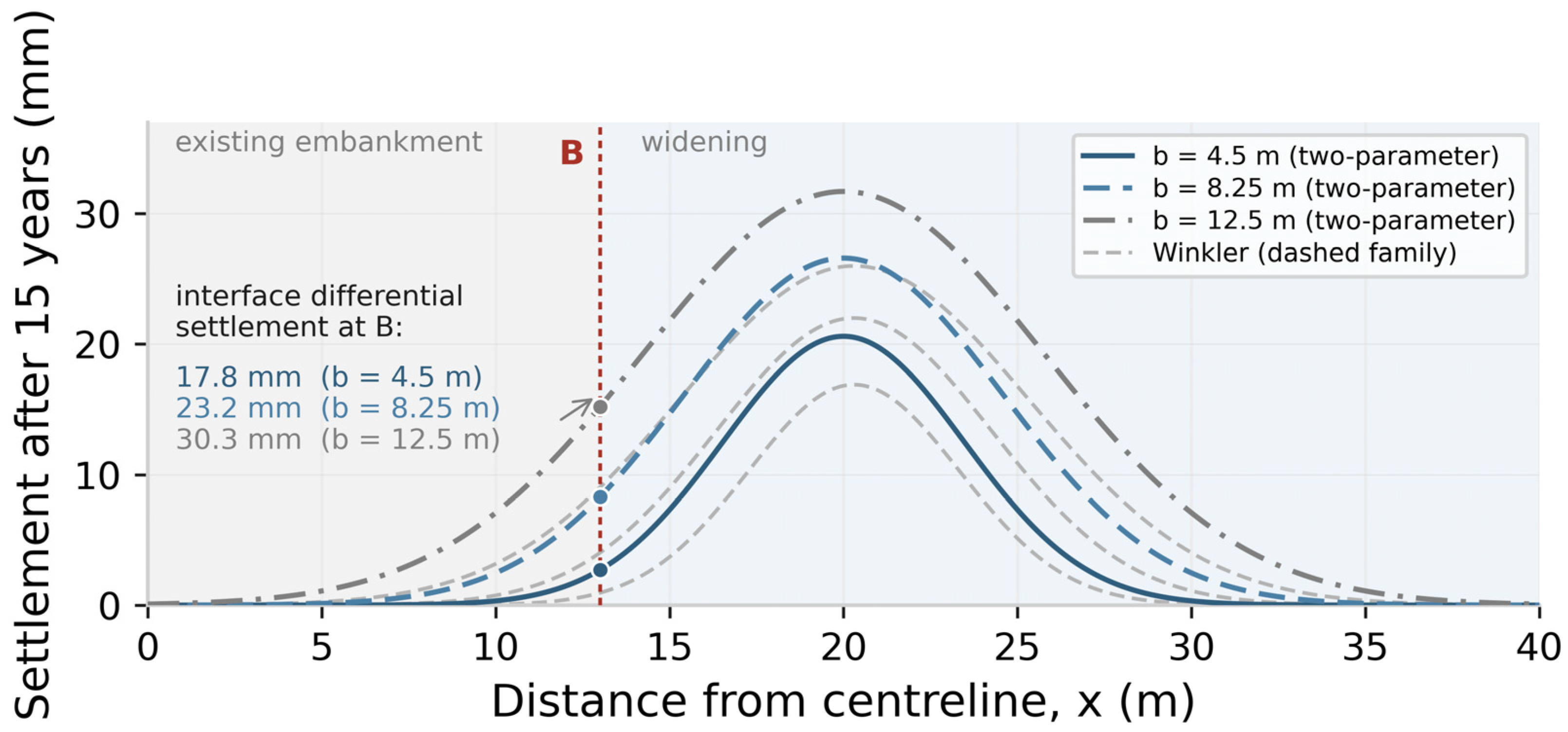
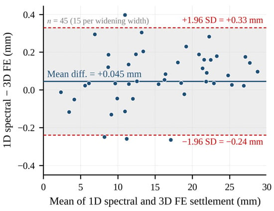
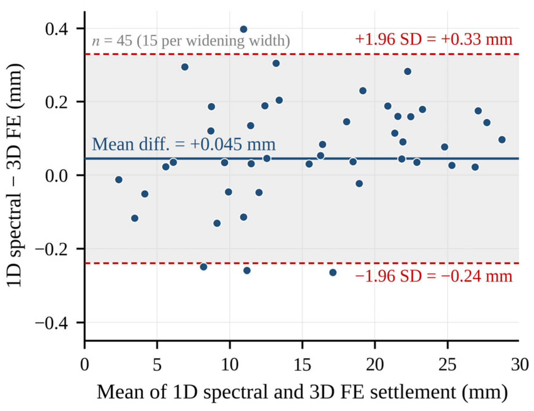
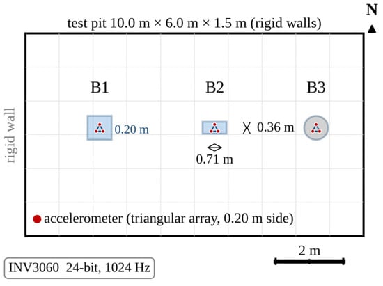
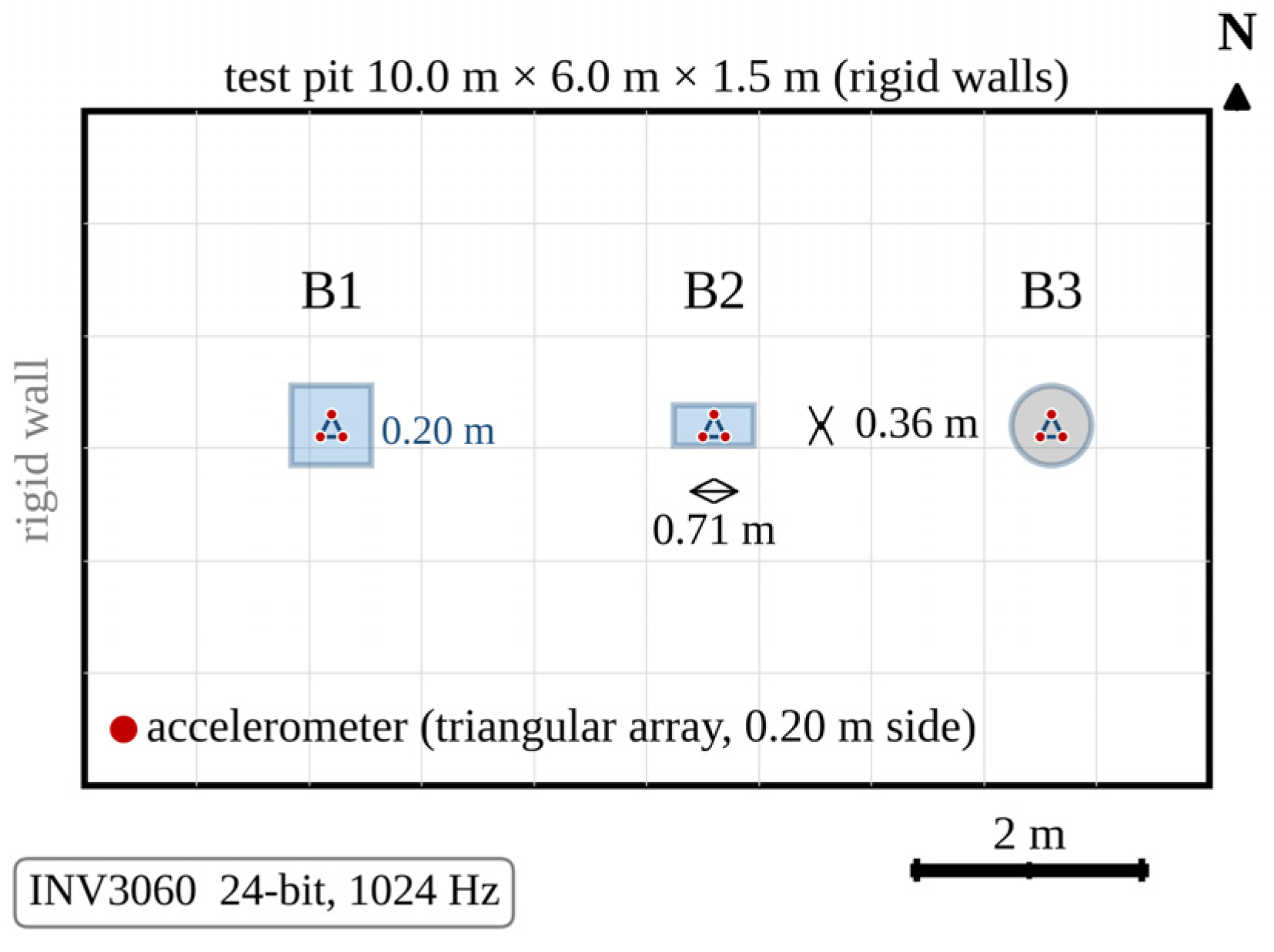
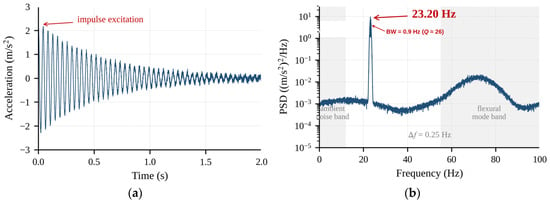
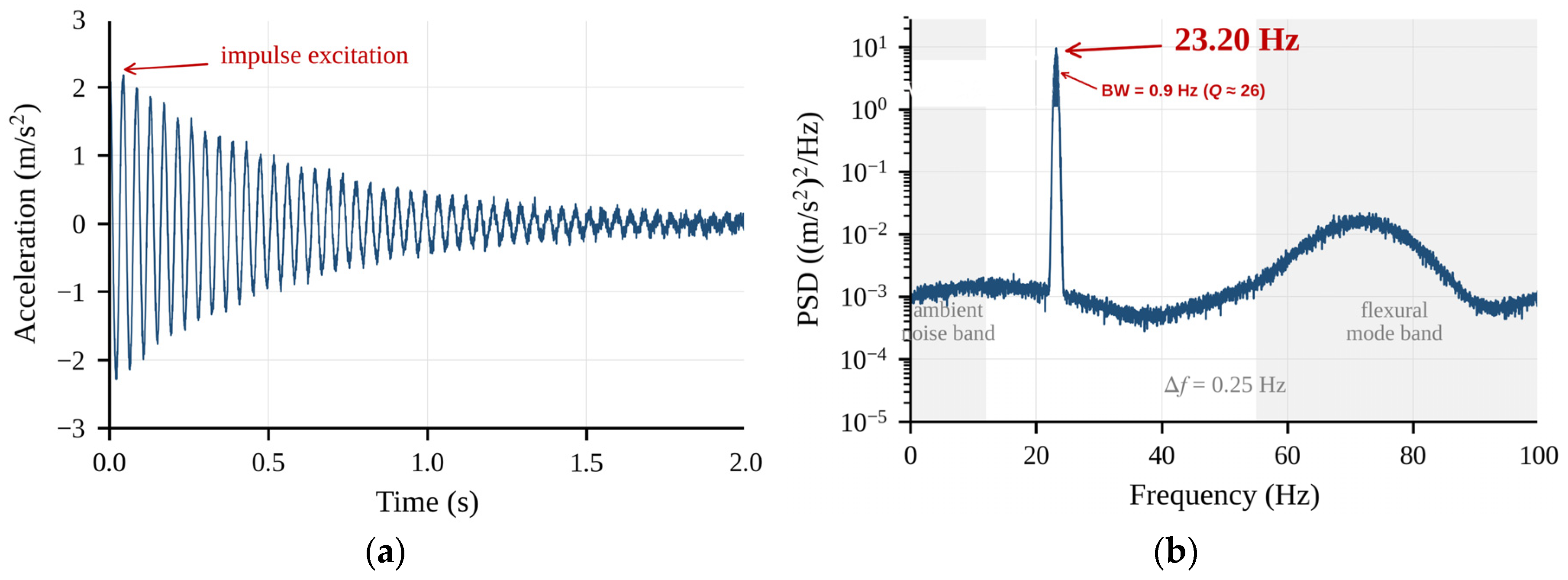
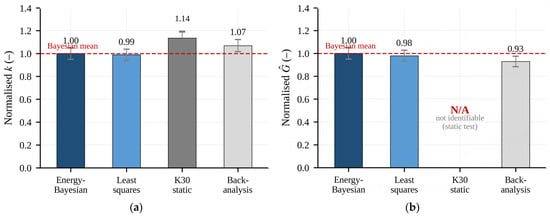
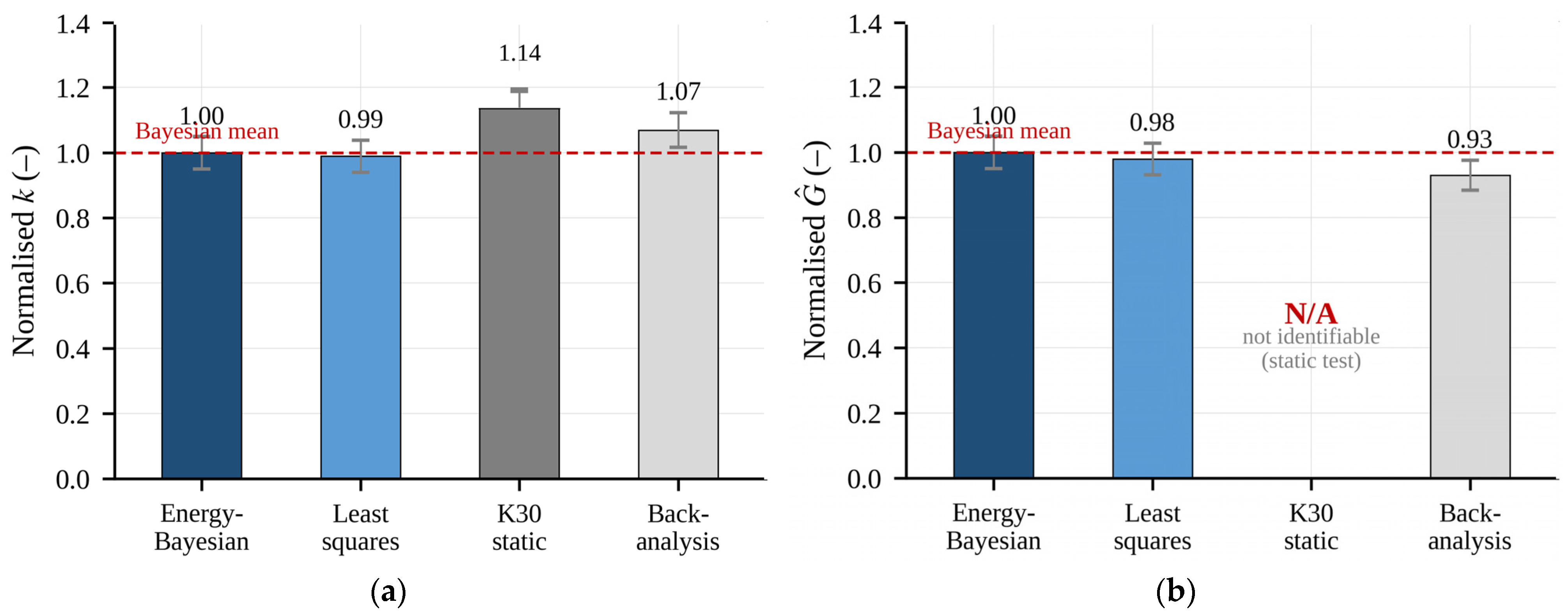
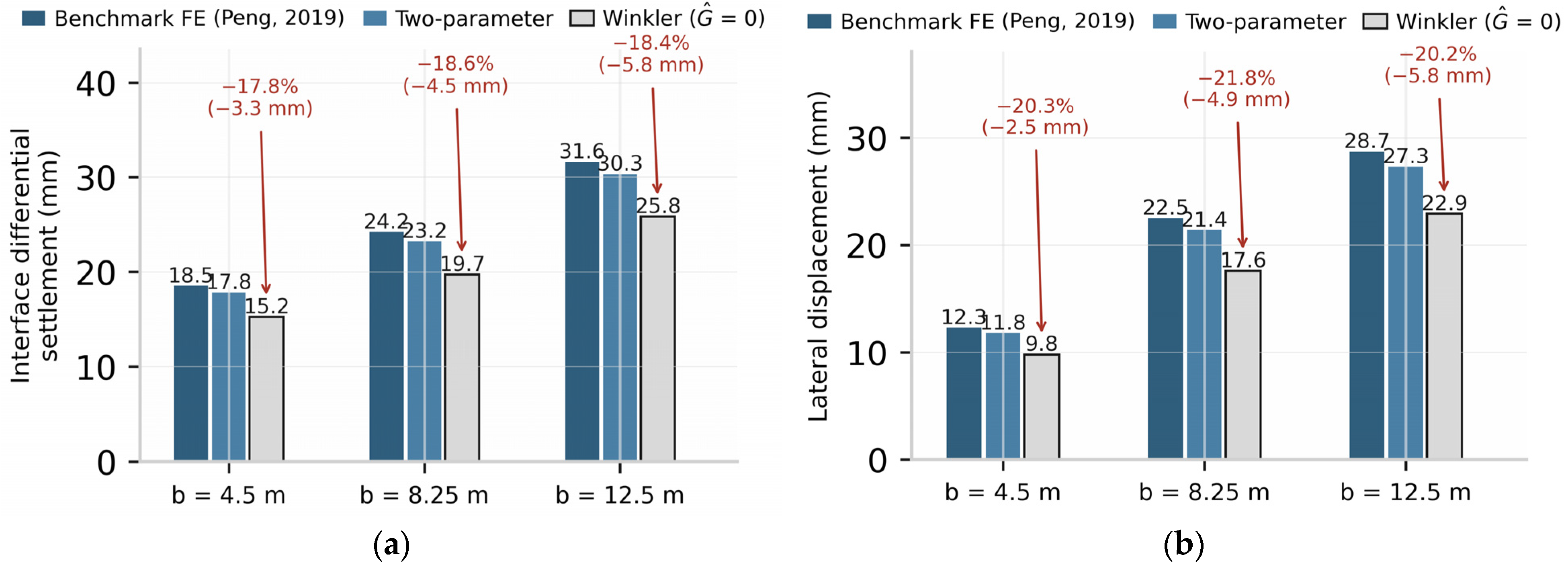
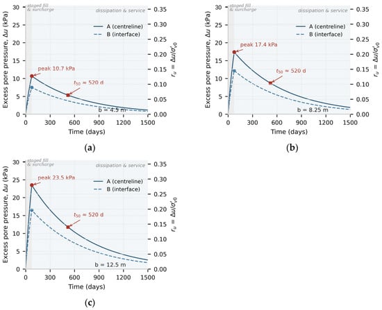
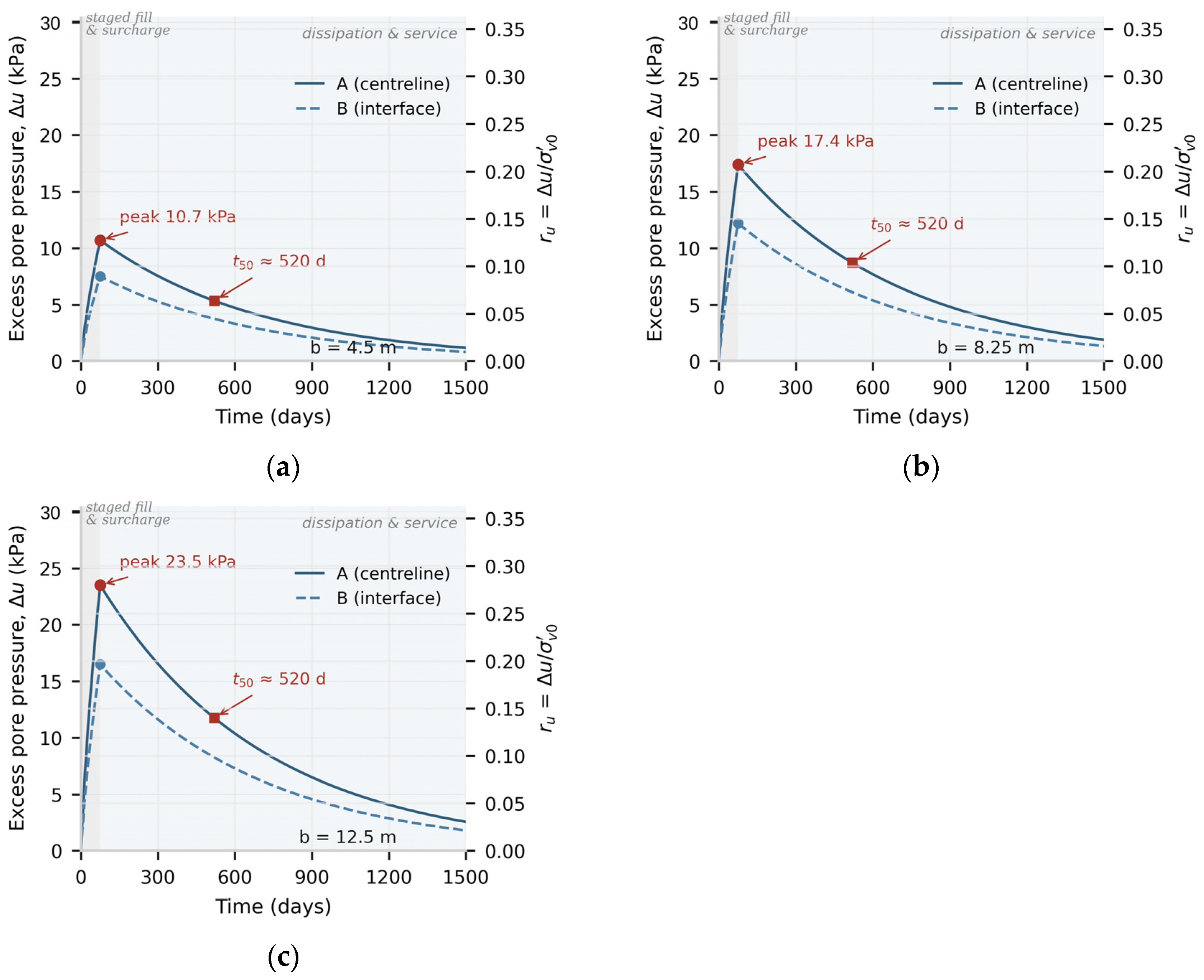
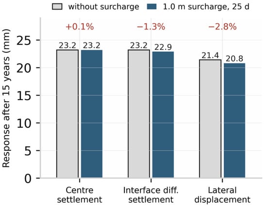

Disclaimer/Publisher’s Note: The statements, opinions and data contained in all publications are solely those of the individual author(s) and contributor(s) and not of MDPI and/or the editor(s). MDPI and/or the editor(s) disclaim responsibility for any injury to people or property resulting from any ideas, methods, instructions or products referred to in the content. |
© 2026 by the authors. Licensee MDPI, Basel, Switzerland. This article is an open access article distributed under the terms and conditions of the Creative Commons Attribution (CC BY) license.