


Abstract
Coherence-based damage indicators enable story-level assessment of reinforced concrete buildings from response measurements alone. Four indicators, the mutual information (MI), the transmissibility modal assurance criterion (TMAC), the accumulated transmissibility coherence (ATC), and a normalized spectral distance, are computed from the transmissibility coherence between floor pairs in the Welch and Morlet wavelet domains and validated against documented per-story stiffness reduction on three cases: a numerical pinching frame, a one-third-scale shake-table frame, and a full-scale five-story building through six damage states. The indicators are ordinal severity measures producing the same ranking under in-band noise to , saturation thresholds of and above, a shorter analysis window, and displacement in place of acceleration. The normalized distance is the most robust severity measure, on the base-to-first-floor path of the numerical case; MI detects onset, falling to 3 to of its estimator ceiling. A measured base channel is the most valuable instrument: the only channel whose removal degrades the severity correlation, and the only path on which the coherence formulation clearly outperforms an elementary amplitude index. Story-level localization requires a sequence of damage states; severity is recovered from base and roof alone.
1. Introduction
Vibration-based structural health monitoring (SHM) infers the condition of a structure from its measured dynamic response. For buildings, two attributes of a damage indicator carry practical weight. The first is output-only operation: the indicator is computed from the responses alone, without a structural model, knowledge of the excitation, or a training phase [1]. The second is story resolution: the indicator identifies which story carries the damage, the resolution a post-event decision on occupancy, retrofit or demolition requires.
This paper asks how much can be learned about the condition of a reinforced concrete (RC) building, story by story, from its vibration responses alone. Four coherence-based indicators are validated against documented per-story stiffness reduction on three RC structures of increasing realism. The evaluation determines the role of each indicator, the sensors needed to locate damage by story, and how the indicators track a building against its own records.
Transmissibility between two floor responses is the ratio of their spectra, so the excitation spectrum, common to both, cancels; what remains characterizes the transfer of motion between the floors independently of the input [2,3]. The indicators are derived from the coherence of that pair, the transmissibility coherence, hereafter TC: the magnitude-squared coherence between two floor responses, the fraction of the power of one that is linearly predictable from the other [4,5]. It is unity when the two floor responses are related by a single linear time-invariant transfer function and the measurement is clean, and it falls in proportion to the power that departs from that description [5]. Normalized by both auto-spectra, it is invariant under the inter-story transfer itself, so it reports the fidelity of the transfer and not its magnitude. Stiffness loss in a reinforced concrete frame lowers that fidelity in three ways. Cracking, bond slip, and pinching make the restoring force history-dependent and spread response power beyond a linear description [6,7]. The secant stiffness falls within the record, so a window spanning the change combines several transfers into one [8,9]. The softened response shifts its power toward lower frequencies against a fixed noise floor [5]. The TC therefore responds to nonlinearity, nonstationarity, and noise, and tracks stiffness loss through them. The TC is estimated with the Welch method, which averages over the record and presumes stationarity, and with the Morlet wavelet coherence, which resolves the estimate in time and frequency through the nonstationary strong-motion segment. Each TC profile is condensed into four scalars by comparison with a baseline profile: the mutual information (MI) [10], the transmissibility modal assurance criterion (TMAC) and the accumulated transmissibility coherence (ATC) [4], and a normalized spectral distance [1,11].
ATC, TMAC, and MI [4,10] were established on laboratory-frame data under stationary excitation, where the Fourier-based formulation proved weak on nonlinear systems. Under seismic excitation, the response is nonstationary and the inter-story transfer changes within the record, so the coherence is estimated in time and frequency. Fan et al. [12] introduced the concept of wavelet transmissibility as a damage onset detector; their formulation used wavelet-domain versions of the structural equations of motion. Dziedziech et al. [8] proposed an alternative formulation in which the wavelet transmissibility is expressed through auto- and cross-wavelet spectra of response signals, and introduced the corresponding wavelet coherence. The present work carries the indicator family into the wavelet domain, applies it to seismic responses of RC frames, and adds the normalized distance [11,13], which responds to changes of level and shape alike and emerges as the strongest severity measure of the four. RC structures are the demanding test bed: cracking, bond slip, and pinching produce strongly nonlinear hysteretic response.
Three data sets form the validation hierarchy. Case I is an incremental dynamic analysis of a three-story RC frame with pinching hysteretic stories, calibrated to the one-third-scale specimen of Bracci, Reinhorn, and Mander [6]: twenty-two analyses under one ground motion at increasing intensity, with the per-story secant stiffness reduction read from the model. Case II is the shake-table record set of that specimen under three scaled Taft motions, with the per-story stiffness reductions identified by the test program [14]. Case III is a full-scale five-story RC building tested fixed-base on a shake table [15,16]: six damaging earthquakes drive it through seven states, DS0 to DS6, of which DS0 to DS5 carry a low-amplitude characterization, the protocol with which Moaveni et al. [17,18] detected stiffness losses in the seven-story building slice tested on the UCSD-NEES shake table, the closest full-scale precedent for this validation; the per-story stiffness reduction was identified from the modal properties [19], and the damage states follow [20].
The contribution of this study is fourfold. First, it ranks the stiffness reduction of each story from response measurements alone and validates that ranking against per-story stiffness references in three RC structures of increasing realism. The indicators are ordinal: they rank damage states on a relative scale. Story-level localization is obtained from the ordering of the indicator along a sequence of damage states. Second, it adds the normalized spectral distance to the indicator family; across all three cases it is the most robust of the four. Third, MI detects damage onset, TMAC and measure severity, and ATC serves within a single path only, and the wavelet estimate is required on the input-anchored path, where the Welch estimate does not track damage. Fourth, it yields instrumentation guidance: severity assessment depends critically on responses at only two levels, base and roof.
2. State of the Art of Transmissibility-Based Damage Indicators
Vibration-based damage detection compares a measured dynamic signature against a reference. The transmissibility function, the ratio of two response spectra, needs no excitation measurement; its estimation in output-only analysis was established by Devriendt and Guillaume [3] and extended to harmonic and colored excitation [21] and to power-spectral-density transmissibility [22,23]. Transmissibility differences carry damage information [24,25,26], band-limited spectral features support statistical detection [11], and the concept generalizes beyond the single-force case [2]. Detection is far more reliable than localization [27], which requires transmissibilities between complete sets of degrees of freedom [28]. Low-cost accelerometers and vision-based measurement have since made floor-by-floor data attainable, which renews the question of how much diagnostic capability response-only data supports.
Zhou et al. [4] proposed the transmissibility coherence as a damage-sensitive feature and introduced ATC and TMAC, which detect the onset of nonlinear behavior while remaining insensitive to linear mass and stiffness changes. The coherence function is a measure of linear time-invariant dependence between two signals, and low coherence between two response signals has been traditionally interpreted as nonlinear structural behavior or measurement noise [5,7]. TMAC applies the cosine similarity of two spectral vectors, a measure since developed into cosine-based and extended indicators [29], hierarchical clustering [30], the weighted transmissibility assurance criterion [31], and a maximum-entropy approximation [32]. Related output-only strategies combine transmissibility with correlation analysis [33], probabilistic distances [13], and entropy measures [34]. For nonlinear structures, transmissibility has been generalized through nonlinear output frequency response functions [35,36].
The stationarity assumption behind Fourier-based transmissibility is the main obstacle to seismic application. The wavelet decomposition, localized in time and frequency, follows the nonstationary response through the strong-motion segment; the transform and coherence follow Torrence and Compo [37] with the smoothing framework of Grinsted et al. [9]. Dziedziech et al. [8] developed the wavelet transmissibility and its coherence in terms of auto- and cross-wavelet spectra of response signals, and showed that they monitor abrupt, damage-related changes under shock loading. No prior study has condensed the wavelet coherence into scalar indicators and validated them against a story-resolved stiffness reduction under strong ground motion. The wave travel-time analysis of Todorovska and Trifunac [38,39] reaches by an independent route the same conclusion on the value of a foundation channel that Section 4.3.5 draws. The band-variable filter of Ditommaso et al. [40,41] follows the migration of the fundamental frequency during strong shaking, and Section 6.1.5 applies it to the Case III records.
Information-theoretic features build on Shannon entropy [42]. Mutual information on continuous data is estimated by histogram methods with principled bin selection [43] or by nearest-neighbor methods [44]. The mutual information between baseline and current coherence profiles was introduced by Tezcan and Marin-Artieda [10], who showed that it detects small linear changes to which ATC and TMAC do not respond. Negentropy-based features for rotating machinery rest on the same premise, that damage alters the statistical structure of the response [45].
Learning-based approaches classify damage from transmissibility data sets with convolutional networks [46], flag reconstruction error of wavelet-transmissibility spectra with autoencoders [47], transfer damage knowledge across structures [48], exploit transmissibility sensitivity in model updating [49], and, on the Case III building itself, predict damage states from vibration records [19]. Self-supervised learning has entered fatigue monitoring [50]. Indicator-based methods remain complementary: transparent, free of training data, and computable in near-real time, they are the baseline-referenced features at the core of statistical pattern recognition for SHM [1]. The literature shows that coherence-based features respond to damage but does not quantify how faithfully they track its severity, which requires a story-by-story damage truth. This study supplies that validation.
3. Methods
3.1. Welch Transmissibility Coherence
Let x and y be the responses of two floors, recorded simultaneously with the mean removed. Each pair of instrumented floors defines one transmissibility path. The one-sided auto-spectral densities and and the cross-spectral density are estimated with the Welch method [51] on Hann-windowed segments with overlap. The transmissibility coherence is the magnitude-squared coherence [4],
the fraction of the response power at frequency f that the two floors share through a linear, time-invariant relationship. Departures from unity arise from nonlinearity, time variation of the system, measurement noise, and the finite averaging of the estimator [4,5]. TC is evaluated on the frequency lines of the analysis band, 0.5 to 10 Hz, which contains the first modes of every structure studied. Each case and path yields one TC profile, the vector of TC values over the in-band lines, and these profiles are what the indicators compare.
The estimator carries a bias [5,52]
where is short for , is its estimate, and K is the number of averaged segments. Cases I and II use segments of samples at overlap, which on their 31.3 s records gives complete segments; Case III uses 2048-point segments on a 120 s window sampled at 50 Hz, . At the bias is (Cases I and II) and (Case III). The bias is smallest on the baseline, where is closest to unity, and largest on the evaluated profile, where the coherence has fallen. It therefore attenuates the measured change, compressing and driving TMAC toward unity; it can only understate damage. For , the mapping of Equation (2) is monotone in , so the order of the coherence values is preserved on every line and MI, invariant to a monotone transformation of both profiles, is unchanged; the attenuation of is bounded by the bias itself, at most and between and unity at .
For a linear time-invariant system driven by a single deterministic input with noise-free measurements, the coherence is identically unity. On a single transient record, an estimate departs from unity only through finite frequency resolution and through nonlinearity or time variation of the system, which make the transfer differ between the averaged segments or scales; the bias of Equation (2) raises it toward unity. For a nonlinear structure, the estimate therefore depends on the excitation as well as on the state, and it is not an ensemble quantity. Two states are compared only under comparable excitation, a condition examined for the Case III sets in Section 6.1.6.
3.2. Wavelet Transmissibility Coherence
For seismic responses, the TC is also estimated in the time-frequency domain, following Dziedziech et al. [8]. The continuous wavelet transform resolves the signal x jointly in scale s and time t with the analytic Morlet wavelet , with a dimensionless time parameter, at [9,37], the value at which the wavelet is admissible and separates the structural modes while remaining localized enough in time to follow the strong-motion response. Scale maps onto Fourier frequency through the Fourier factor of the Morlet wavelet, the ratio of the equivalent Fourier period to the scale s [37],
below the approximation ; all frequencies reported here use Equation (3). The Fourier transform of the wavelet is a Gaussian of relative width , which sets the smallest modal-frequency change the profiles can separate. The wavelet TC is the smoothed wavelet coherence [9,37],
where is the time-and-scale smoothing operator and the asterisk denotes complex conjugation; without smoothing, Equation (4) equals one identically [9]. lies between zero and one. The scale axis is discretized at twenty-four voices per octave. Coefficients outside the cone of influence are discarded [37]. The coherence map is averaged over time at each scale to form a one-dimensional profile. The coherence cannot exceed one, and a line whose baseline value already sits at that ceiling is saturated: it enters every inner product as a constant near one and drowns the lines that change, so lines whose baseline coherence exceeds 0.999 are masked out.
The smoothing operator sets the absolute level of the estimated coherence, and with it, every value of ATC and , so its parameters are stated [9,37]. It is the composition , where smooths along the time axis and along the scale axis. In time, it is a convolution, at each scale, with a normalized Gaussian of standard deviation equal to the scale,
a window of cycles of the analyzed frequency at every scale. In scale, it is a normalized boxcar of width octaves, the scale decorrelation length of the Morlet wavelet at [37], realized at as a fifteen-tap kernel with thirteen unit weights and two end weights of , octave ( to ) about each line.
The saturation threshold is a processing choice, and it is absolute, so the count it retains depends on the measurement noise as well as on the state; both dependences are quantified on Case I in Section 4.3.6 and Section 4.3.7, and the lines surviving both masks are listed by case, path, and domain in Table A4.
This yields a one-dimensional wavelet TC profile over frequency, the same object as the Welch TC profile and processed identically from here on.
3.3. Damage Indicators
Let u be the baseline TC profile of one path, the mean profile over the undamaged cases, and v the profile of the case under evaluation on the same frequency lines, with and their values at the k-th in-band line, . Four scalars condense the comparison of v against u.
3.3.1. Mutual Information (MI)
MI measures the statistical dependence between the two profiles treated as paired samples over frequency [10]. In the Welch pipeline, both profiles are discretized into B equal-width bins and
where is the empirical joint probability that falls in bin i and in bin j, and the marginals, and B follows the low-bias rule of Hacine-Gharbi et al. [43]. The wavelet pipeline evaluates the same functional with the nearest-neighbor estimator of Kraskov, Stögbauer, and Grassberger (KSG), [44], in bits. The masked wavelet profiles retain few samples with marginals concentrated near one, where the histogram estimator admits too few bins and the nearest-neighbor estimator adapts to the local density. The positive finite-sample bias of the KSG estimate is estimated under independence by 200 seeded circular block permutations of the current profile and subtracted (Appendix A). Because the two pipelines use different estimators, MI magnitudes are not compared across domains. MI is reported throughout as a fraction of its own estimator ceiling, bits, with the digamma function, the value the raw estimate returns when the two profiles coincide (Equation (A5)). The ceiling is set by the retained line count and not by the structure, so the normalization divides each path by one constant, gives the value one meaning across paths and buildings, and leaves the onset step and every rank correlation unchanged.
3.3.2. Transmissibility Modal Assurance Criterion (TMAC)
TMAC [4] measures the shape similarity of the two profiles,
It is one when the profiles are proportional, decreases as their shapes diverge, and is insensitive to a proportional rescaling of either.
3.3.3. Accumulated Transmissibility Coherence (ATC)
ATC [4] integrates the level of the current profile over the band,
with Δf the line spacing. On the uniform Welch grid, this is an integral over frequency; on the logarithmic wavelet grid, the median spacing is used and the quantity is, to within a constant, an integral in . The constant leaves rank correlations unaffected. ATC uses the current profile alone and carries no reference to the baseline.
3.3.4. Normalized Spectral Distance
A profile can change in level, when the coherence rises or falls across the band while keeping its pattern, and in shape, when the coherence redistributes over frequency at little change of overall magnitude. TMAC responds to shape only, ATC to the level of the current profile only, and MI can remain high while the profiles drift apart systematically. The distance accumulates the absolute pointwise deviation between the profiles and responds to both. A plain sum scales with the retained line count , which differs with the domain, the mask, and the record length, so every value is normalized by it,
the mean absolute deviation over the retained band. Within a path, is fixed by the baseline mask, so the normalization divides every state by one constant and leaves rank correlations unchanged, while giving magnitudes one meaning across paths, records, and domains. On the logarithmic wavelet grid, the unweighted sum gives every octave equal weight, so the low-frequency octaves that carry the modes count as much as the high-frequency ones; a frequency-proportional weighting would suppress the low-frequency decoherence that damage produces. The absolute deviation is preferred to a squared one, which would let the few large deviations at the modal peaks mask the broadband coherence loss between them. The distance is a metric on the profile space, which TMAC and MI are not; the choice against a squared deviation and a probabilistic divergence is tested in Section 7, where nothing in the results is found to depend on it.
3.4. Processing Workflow
Figure 1 sets out the processing chain from the measured floor records to the four indicators and the severity assessment. The chain is identical for all three cases in the manuscript and both domains.
Figure 1.
Processing workflow from measured floor responses to the four damage indicators and the severity assessment.
3.5. Baseline Referencing and Severity Correlation
Every indicator is evaluated against the documented stiffness reductions with the Spearman rank correlation , since each indicator moves consistently with the reduction but not in proportion to it. The truth vectors contain ties, from cases sharing zero damage and from plateaus, and are handled with the average-rank convention; without tie correction, the coefficients shift by up to 0.05 on these data. The cases within each set are one-motion-scaled to successive intensities on one structure, hence serially dependent, so all coefficients are reported as descriptive effect sizes and not tested for significance. The parameter set, band, wavelet settings, masks, and estimator orders, is applied unchanged across all three cases, both domains and both measurement quantities.
4. Case I. Numerical Study of a Three-Story Frame
Figure 2 shows the prototype from which Cases I and II descend: a three-story RC office building with three 5.49 m bays in the direction of testing, 3.66 m stories, 15.24 cm slabs, 22.86 by 45.72 cm beams, and 30.48 cm square columns, designed for gravity loads only to pre-seismic detailing practice of the central and eastern United States [6]. The experimental specimen is a one-third-scale model of one interior frame, story height 1.22 m, floor weight about 120 kN, total weight about 360 kN, tested under the Taft record at 0.05, 0.20, and 0.30 g [14].
Figure 2.
Layout of the idealized prototype building underlying Cases I and II. Adapted from [6].
The Case I model is a three-degree-of-freedom shear-building idealization of this frame with pinching, degrading hysteretic story springs, the phenomena documented by the experimental program [14]. The spring parameters were calibrated to the measured behavior of the specimen: first-mode frequency 1.81 Hz against 1.78 Hz identified on the undamaged specimen, modal damping 2% in all modes against 2.0, 2.4 and 2.0% identified, story shear 54.3 kN at 0.20 g against 54.7 kN measured. At 0.30 g, the model develops 60.7 kN against 55.2 kN: the specimen holds 0.152 and 0.153 of the model weight at the two intensities; the model rises from 0.151 to 0.168, so the measured strength saturation is not reproduced. The model is a validated, fully documented representation of the nonlinear response of a gravity-load-designed frame; the experiment itself is Case II. Figure 3 shows the computed story-shear against inter-story-drift loops at the moderate and severe intensities. Parameters and implementation verification are in Appendix B.
Figure 3.
Computed story shear against inter-story drift of the baseline frame at 0.20 g and 0.30 g, showing the pinched, degrading hysteresis calibrated to the experimental program.
Figure 4 shows the model under incremental dynamic analysis: the Taft N21E record scaled to twenty-two intensities between 0.025 and 0.30 g, the model analyzed from the undamaged state at each. Drifts are at model scale, story height 1.22 m. In Panel (a), the second story yields first, at 0.083 g, the first story at 0.10 g. The drift is then non-monotonic in intensity, because accumulated degradation lengthens the period and can detune the structure from the energetic band of the record. The third story yields at 0.15 g alone and stays below 4.8 mm elsewhere. The largest drift is 31.3 mm in the first story, 2.6% of the story height; at 0.30 g, the secant stiffness falls 75% in the first story, 74% in the second, and not at all in the third. Panel (b) matches the measured profiles [14] within at 0.05 g and at 0.20 g; at 0.30 g, it runs lower at the roof and higher at the first floor.
Figure 4.
Case I model under the incrementally scaled Taft N21E record. (a) Peak inter-story drift against peak ground acceleration (PGA). (b) Peak floor displacement profiles at 0.05, 0.20, and 0.30 g.
4.1. Three Damage Configurations
Three configurations form a controlled ensemble. The baseline frame carries no prescribed damage. Two localized-damage configurations confine the reduction to one prescribed story. In , the second story starts at 0.70 of its baseline stiffness and 0.90 of its yield strength, and the first and third stories carry overstrength factors of 1.75 and 1.50, respectively, to hold the damage in the prescribed story. In , the third story starts at 0.85 of its stiffness and 0.90 of its strength, with the same overstrength factors on the first and second stories. The parameter is the baseline story stiffness against which reduction is measured. and are not physically realistic; their purpose is to place a known stiffness loss at a known story, which the baseline frame cannot do because its stiffness loss accumulates with strength loss and ductility demand, and they are compared with it qualitatively.
Figure 5 shows the per-story stiffness reduction of the three configurations. Each configuration was analyzed under the Taft N21E record on its own intensity grid, sharing the reference levels 0.05, 0.20, and 0.30 g. The baseline frame uses twenty-two levels capped at 0.30 g, the intensity of the most severe Case II test, so that the numerical and the experimental case cover one range. and use eighteen levels reaching 0.40 g, because the overstrength factors that hold the damage in the prescribed story also require a higher intensity to develop it, which is why the common abscissa of Figure 5 extends to 0.40 g, while the data of Panel (a) stop at 0.30 g, the most severe of the Case II tests that the baseline frame reproduces. In the baseline frame, stories one and two degrade together: story two carries the larger reduction at 12 of the 19 peak ground acceleration (PGA) levels at which damage occurs, story one the larger mean over the grid, against . Story three degrades only at g, by . The stiffness reduction of this frame therefore has two levels, the damaged lower pair and the top story. In , only the second story undergoes stiffness degradation, from 30 to about 64%, stories one and three at zero throughout. In , the third story degrades from 15 to about 66%, stories two and one elastic to g and peaking at stiffness reductions of and , respectively, a factor of at least below the prescribed story at every PGA level. In all three, the reduction is non-monotonic in intensity, an internal control: an indicator responding to intensity alone cannot reproduce a reduction in damage between successive levels.
Figure 5.
Per-story stiffness reduction against peak ground acceleration for the three configurations.
4.2. Incremental Dynamic Analysis and Responses
Each analysis on the three grids of Section 4.1 produces response histories at the three floors. Responses are absolute motions, which retain the ground motion and carry a nonzero base channel, as accelerometers and externally referenced vision systems measure. The severity reference is the per-story secant stiffness reduction, computed exactly by the model at every intensity.
4.3. Results of Case I
Results are reported on absolute accelerations, which correspond to field measurement. Absolute acceleration is the second derivative of absolute displacement, one linear time-invariant filter on both channels of a pair, so the transmissibility and its coherence are unchanged in exact arithmetic. Computed on both, TMAC and agree to the second decimal of their rank correlations in and . MI and ATC differ by up to on the ground path: the weight varies by a factor of five across the -octave smoothing kernel, and neither the smoothing nor the permutation bias correction of MI (Appendix A) commutes with this weight. The model is noise-free; on measured records, the differentiation that relates the two quantities amplifies high-frequency noise, and Case II bounds the effect. Indicators are evaluated on four paths, Gnd–1st, 1st–2nd, 2nd–Roof, and Roof–1st; stories one to three are the segments between successive levels.
4.3.1. Indicator Response at Damage Onset
Figure 6 and Figure 7 show the four wavelet-domain indicators against peak ground acceleration for the baseline frame. Panels (a) and (c) carry Gnd–1st and 1st–2nd, Panels (b) and (d) 2nd–Roof and Roof–1st, with the stiffness reduction overlaid on Panels (c) and (d). Every indicator separates two regimes. Over the elastic levels, MI sits on a plateau, TMAC at unity and at zero on all four paths. The MI plateau is the ceiling of the estimator and not a property of the undamaged frame. In bits, it is path-dependent, to , and it follows the retained line count, which the mask leaves at 96, 93, 65, and 96 on the four paths, with ceilings of , , , and bits. As a fraction of each path’s own ceiling (Equation (A5)), the plateau collapses to 80 to across the four paths of the baseline frame (Appendix A). MI is reported in that normalized form throughout, and no value in bits is used again. At the first yielding level, all four change together, MI, TMAC, and ATC falling and rising, so the onset of nonlinearity appears as a step common to the set. Beyond onset, the trajectories track the overlaid reduction and depart from the monotonically increasing intensity.
Figure 6.
Wavelet domain, baseline frame, MI as a fraction of its ceiling (Equation (A5)), and TMAC against peak ground acceleration. (a,c) Paths Gnd–1st and 1st–2nd. (b,d) Paths 2nd–Roof and Roof–1st. The per-story stiffness reduction is overlaid on the right axis of Panels (c,d).
Figure 7.
Wavelet domain, baseline frame, ATC, and against peak ground acceleration; (a,c) Paths Gnd–1st and 1st–2nd. (b,d) Paths 2nd–Roof and Roof–1st. The per-story stiffness reduction is overlaid on the right axis of Panels (c,d).
MI is the onset detector, and Figure 8 shows the detection independent of where the damage forms. On the Gnd–1st path, across the three configurations, MI holds its plateau at 75 to 80% of its own ceiling (Equation (A5)) while the response is elastic and drops to 15 to 25% at first yield, a step of 55 to 64 points, at 0.083 g in the baseline frame, 0.163 g in , and 0.200 g in . Its power as a severity ranker beyond onset is limited.
Figure 8.
Mutual information on the wavelet Gnd–1st path, as a fraction of its ceiling (Equation (A5)), against peak ground acceleration for the three configurations; dotted lines mark first yield.
4.3.2. Severity Ranking Across Damage Location
Figure 9 gives, for each indicator and path in the three configurations, the tie-corrected Spearman correlation between the indicator and the stiffness reduction of the damaged story. Coefficients are reported with their sign throughout, because the sign carries the ATC finding; denotes a magnitude. The signs are those of the correlations, not of the indicators; TMAC, ATC, and are non-negative by construction, and the bias-corrected MI can take small negative values near independence, down to of its ceiling on the ground path and on Roof–1st, at three intensities each.
Figure 9.
Wavelet domain, signed tie-corrected Spearman rank correlation of the four indicators against the reference stiffness reduction: (a) the baseline frame, referenced to story one; (b) , in which only the second story degrades; (c) , in which the third story is the most damaged.
Two indicators rank severity with a fixed sign at every damage location. The correlation is positive on all twelve path–configuration combinations, to , and at least on every path spanning a damaged story. The TMAC correlation is negative on all twelve, to , and to on the ground path. The MI correlation is on the baseline ground path and weakens to and on the ground path of and , consistent with an onset detector. The ATC correlation is to on the Roof–1st path in all three configurations, but its sign varies with the path: one path inverts in the baseline frame and in , two in , to between and . Each inverted path spans a story that is not the most damaged. This path-dependent sign rules ATC out as a global severity index; its magnitude tracks the states within one path and one estimation domain, the only use retained for it.
4.3.3. The Input-Anchored Path: Wavelet Versus Welch
TMAC and from the two estimators agree within on the three floor-to-floor paths of the baseline frame and diverge on Gnd–1st in every configuration, where the wavelet estimate tracks damage and the Welch estimate does not (Figure 10); in and , the Welch estimate also falls short on 2nd–Roof, by up to . With the wavelet estimate, TMAC and reach 0.82 to 0.96 in magnitude in every configuration; with the Welch estimate on the same data, TMAC, ATC, and fall below 0.55 in the baseline frame and and are informative only in . The Welch estimate averages over the whole record and dilutes the short, strongly nonlinear segments where the pinching response departs from the input; the wavelet estimate retains them. On the input-anchored path under seismic response, the wavelet estimate is therefore a requirement.
Figure 10.
Ground-to-first-floor severity correlation of the four indicators, wavelet against Welch, on absolute accelerations for the three configurations (a–c).
4.3.4. Tracking the Stiffness Reduction and Locating the Damage
Figure 11 follows along the PGA axis against the reference-story reduction on the Gnd–1st, 2nd–Roof, and Roof–1st paths for the three configurations. On every path, it rises from the elastic plateau at onset, follows the reduction as the damaged story softens, and reverses at the level-to-level dips. The reversals are the decisive test, the only points where a response to the structural state and a response to the intensity point in opposite directions. The sharpest change is observed in the baseline frame, where the stiffness reduction in story one falls from 39.2% at 0.100 g to 10.5% at 0.117 g as the ground motion is scaled up; across it, on the ground path falls from 0.081 to 0.046, MI rises from 16 to of its ceiling, and TMAC from 0.969 to 0.995. The indicators reverse with the damage: they track the structural state, not the intensity.
Figure 11.
Wavelet domain, on three paths, left axis, with the reference-story stiffness reduction, right axis, against peak ground acceleration: (a) the baseline frame, (b) , (c) .
The single-story paths localize the damage over height, because a path responds most strongly when the damaged story lies close to the floors the path connects. The 2nd–Roof path shows this across the ensemble: as the prescribed damage moves upward from story one to story three, its correlation rises monotonically, as shown in Figure 9, from in the baseline frame through in to in , where it spans the damaged story itself. The input-anchored path stays high wherever the damage sits, , , and ; what the base channel contributes is taken up in Section 4.3.5. The Roof–1st path, which spans two stories, stays between and throughout. The localization result rests on the end-to-end swing of the 2nd–Roof path, between the configuration in which the damage is furthest from it and the one in which it spans the damaged story, obtained with the same indicator and the same record. The configurations differ in the intensity grid and in the overstrength assignment as well as in the location of the prescribed damage, so the swing measures location sensitivity within a controlled ensemble rather than the effect of location in isolation. It is seven times the margins between paths within one configuration, in and , which are not resolvable over eighteen serially dependent levels and from which no conclusion is drawn. This criterion orders the paths by their rank correlation across the sequence of PGA levels and requires that sequence; the criterion available after a single earthquake, the magnitude of across paths at one state, is evaluated in Section 6.1.2.
4.3.5. The Need for a Measured Ground Input
The localization of the previous subsection anchors each path to the measured base motion, and so requires a reference channel at the foundation. Without it, only floor-to-floor pairs remain, and both channels of such a pair carry the nonlinear response of the whole structure, so the decoherence is not confined to the stories the pair spans and every path reports the whole-building state. Figure 9a quantifies the loss: the correlation of on the input-anchored path falls to and on the 1st–2nd and Roof–1st paths, respectively. The TMAC correlation values follow a similar reduction in absolute value, from on the input-anchored path to values between and on the floor-to-floor paths. Severity is still ranked without the base channel; the ranking no longer carries a location. The model uses the exact ground motion with no measurement noise; Section 4.3.6 tests these values under noise. Case I establishes the mechanism under a prescribed single-story loss and a noise-free input and response; Cases II and III test it on measured records.
4.3.6. Sensitivity of the Input-Anchored Path to Measurement Noise
Gaussian noise, band-limited to –10 Hz, was added independently to the base and to each floor channel at in-band root-mean-square levels of 1, 2, 5, and , twenty realizations per level, each realization one independent draw of noise on every channel of every record; band-limiting the added power is the conservative choice. Two noise models apply. In the first, the added rms is a percentage of each channel’s own in-band rms, so every channel carries the same signal-to-noise ratio. In the second, it is one absolute rms on every channel, set by the roof, as a fixed instrument noise floor gives; the base channel’s in-band rms is of the roof’s on these records, so this model loads it times harder. Each model appears twice: with the baseline profile and the saturation mask recomputed from the noisy records, as they would be obtained in practice, and with both held at their noise-free values, which separates the noise from the changing line set.
The severity ranking on the input-anchored path is unaffected. The rank correlation of is noise-free and , , , and at the four levels under own-channel noise (Figure 12a), and at and at under a fixed noise floor; TMAC stays between and . The 2nd–Roof path, which spans no damaged story, swings by and has no severity information to preserve.
Figure 12.
Measurement-noise sensitivity of Case I. (a) Severity correlation of and (b) retained lines, both for own-channel noise with the threshold recomputed. (c) Margin, for both noise models and both mask treatments. Error bars: one standard deviation over the realizations in (a), twice the standard error of the paired difference in (c).
The margin is the rank correlation of on the input-anchored path minus that on the best floor-to-floor path, the latter fixed at each level by its mean over the realizations. It measures what the base channel is worth, and the two mask treatments give different answers for it (Figure 12c). With the line set held fixed, the margin holds, noise-free and at under a fixed noise floor. With the threshold recomputed, it falls to under own-channel noise and reverses to under a fixed noise floor. Figure 12b gives the cause: noise pushes the near-saturated baseline lines of the floor-to-floor paths below the threshold, and the retained count rises from 93 to 104 on 1st–2nd and from 65 to 104 on 2nd–Roof. Those released lines carry little severity information but are counted, and the path improves from to ; with the same lines held fixed, it degrades to , as an increase in noise must.
Noise itself therefore does not erode the value of the base channel within in band. The absolute saturation threshold does, releasing lines in proportion to the noise, and under a fixed instrument noise floor at that is enough to reverse the ranking of the paths. Within a realization, the same draw perturbs both paths of a comparison, so margins are resolved against twice the standard error of the paired per-realization difference.
4.3.7. Sensitivity to the Saturation Threshold
The saturation threshold of Section 3.2 is a processing choice: the mask discards every line whose baseline coherence reaches it. Its influence was measured by repeating the Case I analysis at , , , and with no mask, on all four paths and the 22 intensity levels, in the wavelet domain on absolute accelerations, each setting scored by the tie-corrected Spearman correlation against the documented stiffness reduction in the reference story (Table 1).
Table 1.
Saturation-threshold sensitivity of Case I. is the number of the 104 in-band lines entering the indicators. The column carries the sampling variability of the 200-permutation bias correction of MI (Appendix A), about ; the adopted rows are those of the deposited run, from which every MI value in the text is quoted.
At , the mask retains 96, 93, 65, and 96 of the 104 in-band lines, so the retained count is a property of the path, which is why Equation (9) is normalized by it. Between and no mask, moves by at most , the least of the four indicators, against for ATC, for TMAC, and for MI, which follows the retained count (Appendix A). At , which discards up to of the band, TMAC and shift by and on the 1st–2nd path. A mask should remove only lines at the ceiling, so is adopted. The sign of the ATC correlation is stable under the sweep and differs between paths.
5. Case II. Evaluation of the Indicators Using Experimental Data from the Three-Story Shake-Table Tests
The test bed is the one-third-scale three-story RC frame of Bracci, Reinhorn, and Mander [14], the specimen that calibrated the Case I model. It was subjected to three shake-table tests under the Taft N21E record scaled to 0.05, 0.20, and 0.30 g, producing an essentially elastic, a moderately inelastic, and a severely inelastic response. Displacement transducers measured the absolute horizontal displacement of the base and of each story at 100 Hz for about forty seconds per test, and the four paths of Case I are formed from them: Gnd–1st, 1st–2nd, 2nd–Roof, and Roof–1st.
The severity reference is the per-story stiffness identified by the program itself from white-noise tests at 0.024 g after each earthquake test [14]. Figure 13 summarizes it. The story stiffnesses fall from 8.8, 9.5, and 9.4 kN/mm undamaged to 5.0, 3.9, and 4.3 kN/mm after the severe test. The cumulative reductions in the first, second, and third stories are 10.7, 13.1, and 12.4% after the minor test, 42.9, 42.6, and 32.0% after the moderate test, and 43.3, 58.8, and 53.6% after the severe test. The first-mode frequency falls from 1.78 Hz through 1.71 and 1.42 to 1.20 Hz. The reference test itself already carries a 10.7 to 13.1% reduction: an RC frame has no truly undamaged state, since shrinkage and construction leave the sections cracked and the 0.05 g shaking initiates further flexural cracking. All indicators therefore measure change relative to a lightly cracked state.
Figure 13.
Case II damage reference, from the white-noise identification after each test. (a) Story stiffness, (b) cumulative reduction from the undamaged state, (c) first-mode frequency.
The identified stiffnesses and frequencies come from the same tests and are mutually consistent. A shear-building eigenvalue solution from the identified story stiffnesses, with uniform floor masses, predicts first-mode frequency ratios , damaged over undamaged, of 0.940, 0.762, and 0.701 after the three tests, against the measured 0.961, 0.798, and 0.674, within 2 to 5%. The model-free relation gives 54.6% for the severe test against a mean identified per-story reduction of 51.9%.
The indicators are computed exactly as in Case I: the same 0.5 to 10 Hz band, Welch settings, Morlet settings, and masks. The three records are truncated to 3126 samples (31.3 s), the shortest of the three, so the estimates average over equal durations. The window contains the whole motion, the roof response of the severe test reaching of its energy by s, and its influence is bounded with the results below. The reference profile of each path is the 0.05 g test, so every indicator measures change relative to the least-damaged available state; the truth is expressed relative to the undamaged state, a monotone change of scale that leaves the ranks unchanged.
5.1. Results of Case II
Figure 14 and Figure 15 show the four wavelet indicators on the four paths across the three tests, with the measured reduction overlaid. Three findings of Case I replicate. First, MI drops at the first damaged test on every path, from 80 to 89% of its own ceiling (Equation (A5)) to 8 to 12%, and is not monotone beyond it, the 1st–2nd value rising from to between the two damaged tests: an onset detector. Second, TMAC falls and rises with the measured damage on all four paths, TMAC on Gnd–1st from unity through 0.919 to 0.858 and from zero through 0.135 to 0.181; the largest response is on Roof–1st, which spans two stories, reaching 0.206. The severity ordering carries over to measured responses up to a 59% story reduction; each damaged test is read against the reference as one pre- and post-event pair. Third, every path responds in proportion to the reduction it spans. Between the moderate and severe tests, the first-story stiffness is nearly unchanged, falling from to kN/mm ( to reduction), while stories two and three lose a further 16 and 22 points; over that increment, the Gnd–1st indicators still move, TMAC from 0.919 to 0.858 and from 0.135 to 0.181. With the whole frame softening, the input-anchored path reports the global state as well as its own story. Case II therefore confirms the onset signature and the severity ordering on measured data; story-local sensitivity of the input-anchored path rests on Case I, where the damaged story is prescribed.
Figure 14.
Experimental shake-table tests, MI and TMAC across the three tests. Panels (a,c) show the Gnd–1st and 1st–2nd paths, Panels (b,d) the 2nd–Roof and Roof–1st paths; the measured reduction in the spanned stories is overlaid on Panels (c,d).
Figure 15.
Experimental shake-table tests, ATC and across the three tests; layout and overlay as in Figure 14. Panels (a,c) show the Gnd–1st and 1st–2nd paths, Panels (b,d) the 2nd–Roof and Roof–1st paths; the measured reduction in the spanned stories is overlaid on Panels (c,d).
The window is not load-bearing: shortened to , , or s, the retained count stays at 103 or 104 on every path, moves by at most , and TMAC by , and the severe test stays separated from the moderate on every path.
Interchangeability of displacement and acceleration was verified on these records: the measured displacements were converted to accelerations by numerical differentiation, using the second-order central-difference formula for the second derivative, and every indicator recomputed. Differentiation applies one common linear filter to both channels of a pair, so exact invariance is expected, and the agreement is close to it: the retained count changes by at most one line on one path, by at most and TMAC by . The ordering is preserved on every path at both damage levels, the moderate-to-severe separation on the displacement series exceeding the larger of the two discrepancies by at least times for and for TMAC. The differentiated series read marginally more damaged on every path, the signature of the high-frequency noise that differentiation amplifies. Displacement and acceleration are interchangeable to within the noise; where a choice exists, the less differentiated quantity is preferable. Under both perturbations, the shortened window and the differentiation, shifts less than TMAC.
5.2. Wavelet and Welch Estimators
Figure 16 compares the two estimators on Gnd–1st with the first-story reduction overlaid. They agree on the direction of every severity indicator: as the reduction rises from 10.7 to 43.3%, MI drops, TMAC falls, and rises under both, so the onset signature and the severity ordering are independent of the estimator. Two damaged states test direction only; the separation seen in Case I requires the intensity sweep. ATC is the estimator-dependent quantity: it decreases under the wavelet estimate and rises between the moderate and the severe test under the Welch estimate.
Figure 16.
Experimental shake-table tests, Gnd–1st path. The four indicators across the three tests, wavelet estimator (top row (a–c)) and Welch estimator (bottom row (e–g)); L1 panels (d,h), the first-story reduction is overlaid on the panels.
6. Case III. Full-Scale Five-Story RC Building
The specimen is a five-story reinforced concrete building tested fixed-base on the outdoor shake table of the University of California San Diego [15,16]. Six earthquakes of increasing intensity drove it from the undamaged state DS0 through the documented damage states DS1 to DS6, the last state fracturing longitudinal bars in the floor beams; a low-amplitude white-noise or pulse test characterized the state after each of the first five. Table 2 lists the sixteen tests in order; the records are in the public archive [53]. Longitudinal accelerations were recorded at the four corner columns of six levels: the base slab fixed to the table, which recorded the input, the four floors, and the roof. Corner records of inverted polarity, documented for the archive [53], are aligned in sign, and the four corners of each level are averaged into the translational motion of the diaphragm. The averaging removes the torsional component by construction, a declared limitation: an indicator on the diaphragm mean would not register a purely torsional change. It is reasonable for this uniaxially driven specimen, and the per-corner analysis below reproduces the ranking at each corner; it should not be carried to plan-irregular structures without re-examination. The six levels define five single-story paths, Gnd–1st, 1st–2nd, 2nd–3rd, 3rd–4th, and 4th–Roof, the first anchored to the foundation record.
Table 2.
Case III, first-mode frequency and equivalent damping of every test, identified from the base-to-roof transfer function.
Figure 17 shows three of the tests, the undamaged characterization DS0, the earthquake FB4 and the characterization DS5, as recorded acceleration and wavelet power below 3 Hz. The first-mode frequency of every test, identified from the base-to-roof transfer function (Table 2, procedure in Section 6.1.5), falls from 1.26 Hz at DS0 to 0.47 Hz during FB6 (Figure 18b), and it falls with the amplitude of the motion: the DS1 pulse test identifies at 1.11 Hz, and the change the indicators register at DS1 carries the different excitation together with the softening. Throughout this work, “per-story stiffness reduction” therefore denotes the reduction in the effective secant stiffness at the amplitude of the test.
Figure 17.
Three of the sixteen Case III tests, recorded acceleration (top) and wavelet power below 3 Hz (bottom): the undamaged characterization DS0, the earthquake FB4, and the characterization after FB5 (DS5). The panel border color indicates the damage state, and the dashed line is the first-mode frequency of Table 2.
Figure 18.
Case III damage reference: (a) per-story secant-stiffness reduction identified in [19]; (b) first-mode frequency versus damage state from the base-to-roof transfer function (Table 2), DS6 from the FB6 record.
The severity reference is the effective story secant stiffness at each state, identified in the authors’ prior study [19] by matching a five-degree-of-freedom shear-building model to the first five modes extracted from the test records with NExT-ERA, and expressed as the per-story stiffness reduction relative to DS0 (Figure 18a); the states follow Astroza et al. [20]. Stories four and five stay at baseline throughout; stories one and two soften from DS1 and story three from DS3, their secant stiffnesses falling from 76.5, 46.8, and 46.4 kN/mm at DS0 to 11.1, 6.8, and 9.3 kN/mm at DS6, reductions of about 85.5, 85.5, and 80%. The severity correlation, the tie-corrected Spearman coefficient of each indicator against the own-story reduction over the states, is therefore computed on the three lower paths only; none is defined against the constant zero reduction of the upper two. The identified modal properties of the building [54], its pretest nonlinear finite-element model [55], and the Bayesian updating of that model [56] are the independent terms of comparison for this reference.
Each record is resampled from 200 to 50 Hz and a fixed 120 s maximum-energy window is extracted, so that quiet lead-in and tail segments do not dilute the estimates. The band is 0.5 to 10 Hz; its lower edge is reached only during FB6, where the fundamental frequency lies below it for of the window (Section 6.1.5), and since the longest period is the most attenuated by the cone-of-influence mask, the FB6 indicators rest on the higher-frequency content of the band and any change concentrated at the fundamental frequency is understated, on the conservative side. Because the records are strongly nonstationary, the reported indicators are computed in the wavelet domain, at with both masks, and MI uses the KSG estimator with the seeded permutation bias correction.
6.1. Results of Case III
The four indicators are read from the five floor-averaged paths, each referenced to its own DS0 value in the white-noise set and to its FB1 value in the earthquake set, and the severity correlation is evaluated on the three lower paths. The Gnd–Roof path, the four corner lines separately, and a Welch counterpart were also computed; the per-corner results reproduce the ranking at every corner and are confirmatory.
6.1.1. Severity Ranking Along the Damage States
Along the white-noise progression (Figure 19 and Figure 20), every indicator moves in the expected sense, rising and MI and TMAC falling, while ATC stays comparatively flat. The trajectories are irregular: MI and TMAC drop at DS1, recover across DS2 and DS3 and fall again toward DS5, and mirrors them, because the set is interspersed with pulse tests. The ten characterizations map onto the six states as one white-noise test at DS0, one pulse test at DS1, two pulse tests each at DS2 and DS3, and two white-noise tests each at DS4 and DS5, plotted as the mean per state, so consecutive states are not driven by equivalent excitation. All ten are retained so that every state is represented. is the clearest indicator in this set, responding over the widest range, and its coefficients of to reflect departures that coincide with the pulse tests.
Figure 19.
Case III, white-noise set: floor-averaged MI (a,b) and TMAC (c,d) against damage state. (a,c) paths spanning softened stories, with the documented reduction overlaid on (c); (b,d) paths spanning intact stories.
Figure 20.
Case III, white-noise set. Floor-averaged ATC (a,b) and (c,d); layout, path groups and overlay as in Figure 19.
Along the six earthquakes FB1–FB6 (Figure 21 and Figure 22), one per state, the indicators follow the documented reduction smoothly and completely: rises in a tight bundle, MI and TMAC fall steadily, and even ATC drifts downward. This set is nonetheless the weaker evidence. Its magnitudes carry the instantaneous softening during shaking together with the accumulated damage, whereas the low-amplitude characterizations isolate the residual state that a post-earthquake assessment asks about. The intensity of FB1–FB6 grows with the damage state it induces, so on this set alone, a correlation with the stiffness reduction cannot be distinguished from a correlation with the shaking intensity. The white-noise set, despite its irregular trajectories and lower coefficients, is therefore the pertinent evidence for the residual state.
Figure 21.
Case III, earthquake set. Floor-averaged MI and TMAC along the damage progression produced by FB1–FB6 (DS1–DS6), one test per state, same layout and overlay as Figure 19. Case III, white-noise set: floor-averaged MI (a,b) and TMAC (c,d) against damage state.
Figure 22.
Case III, earthquake set. Floor-averaged ATC and , same layout and overlay as Figure 19. Case III, white-noise set: floor-averaged MI (a,b) and TMAC (c,d) against damage state.
Figure 23 gives the tie-corrected Spearman correlation of each indicator with the own-story reduction, over the ten characterizations and over the six earthquakes. Both truth vectors carry ties, ten characterizations mapping onto six states and stories one and two sharing a reduction, which cap the attainable coefficient at to . In the white-noise set, and TMAC are strongest at to , MI reaches to , and ATC to ; the earthquake set returns uniformly higher coefficients, and ATC at to , and to with FB1 excluded, but measured on a set in which intensity and state advance together. On every damaged path in both sets, no indicator ranks above ; TMAC ties it under white noise and ATC under earthquake excitation, but alone holds the widest range across both, with a sign that is fixed in every case. MI marks onset reliably and ranks severity least regularly; ATC’s jump from weakest to among the strongest between the sets is the clearest contrast in the figure, and its path- and estimator-dependent sign precludes its use as a stand-alone severity index.
Figure 23.
Case III, signed tie-corrected Spearman correlation between each indicator and the own-story secant-stiffness reduction, on the three paths spanning softened stories (a,b). No coefficient is defined on 3rd–4th and 4th–Roof, whose stories stay at baseline.
Among the three damaged paths, Gnd–1st is nominally strongest in the white-noise set, on both and TMAC against and on 1st–2nd and on 2nd–3rd, but a moving-block bootstrap, block length three, 5000 resamples, places every pairwise difference across or against zero: +0.025 [0.000, +0.180], +0.095 [−0.150, +0.682], and +0.070 [−0.150, +0.566]. The ordering is a point estimate and no base-channel advantage is claimed from it. In the earthquake set, the three paths are indistinguishable on , to , while on TMAC, Gnd–1st leads at against and . Case III therefore validates the severity ranking and the separation of damaged from intact stories over height, stories one to three losing 80 to 85.5% of their stiffness while four and five stay at baseline; where the tie cap binds, the comparison between paths is indeterminate.
6.1.2. Localization from a Single Post-Event State
Localization from a single post-event state fails. After one earthquake, the only statistic available is the vector of across paths at that state; ranked against DS0, it identifies the most-reduced story at two of nine white-noise states and one of five earthquake states, and per corner at one of nine. The corner averaging is not the cause: the mean indicator on the damaged paths exceeds that on the intact paths by a factor of on average in both representations, range to (Figure 24). Story-level localization is therefore established by the ordering of correlations along the sequence of states, not from a single state.
Figure 24.
Single-state localization on Case III, white-noise set. (a) Normalized of each path at every characterization, the largest of the five starred. (b) Mean on the three damaged paths over the mean on the two intact paths, floor-averaged and per corner.
6.1.3. Reduced Instrumentation
Two instrumented levels suffice for severity assessment. The analysis was repeated on subsets of the six levels, each path correlated against the mean reduction in the stories it spans. The best severity correlation is on the full array, on a four-level array of base and alternate floors, on base, second floor and roof, and on base and roof alone. The values coincide because the rank correlation depends only on the ordering of the states, and every array that retains the base orders them identically. Removing the base instead, keeping all five floors, falls to , a larger loss than from removing four floors. Coarse localization reproduces the truth on the four- and three-level arrays and not on the full array. The coarser arrays are not more informative: they pose a coarser question, which the indicator can answer, while the full array asks for the adjacent-story discrimination that Section 6.1.2 has already shown it cannot deliver (Table 3). The base channel is the necessary instrument, and a coarse array suffices for story-level localization.
Table 3.
Severity correlation of on Case III under reduced instrumentation, and of against an amplitude-only benchmark on the transmissibility magnitude, by path.
6.1.4. Frequency Migration and Whole-Building Severity
is not a repackaged frequency shift. The fundamental frequency drops from 1.26 Hz at DS0 to 0.62 Hz at DS5, the mean of its two characterizations and 0.60 Hz on the record of Figure 25, about four wavelet bandwidths (), so on a fixed frequency grid, the baseline and the damaged profile place their modal features at different lines, and the dips near anti-resonances and in low signal-to-noise bands migrate with them. Two tests bound that contribution (Figure 25).
Figure 25.
Case III, white-noise set. (a) Wavelet transmissibility coherence on Gnd–1st: the DS0 baseline at 1.26 Hz, the DS5 record at 0.60 Hz on the fixed grid, and the same DS5 profile mapped by Equation (10); the shaded band is 0.8–1.6 Hz and the dotted line 1.8 Hz. (b) Tie-corrected Spearman correlation of with the own-story stiffness reduction on the three paths spanning softened stories, for the whole band and for the 0.8–1.6 Hz window on each abscissa, for the band with that window deleted, and for the lines above 1.8 Hz.
First, the comparison was repeated on the abscissa normalized by the current fundamental frequency,
which aligns the profiles on their fundamental frequencies. Within one bandwidth of the fundamental frequency, 0.8–1.6 Hz, the aligned distance is state-independent, to on Gnd–1st against to on the fixed grid, and the aligned correlations fall to , , and , from values above on all three paths; half-widths of 0.1 to 0.5 octave about give at most. In that band, the content of is the migration of the fundamental frequency. Over the whole band, the single-ratio map is not exact, because the higher modes of a structure with localized damage do not migrate by the ratio of the fundamental frequencies, and the aligned correlations fall to , , and : there, the map measures the misalignment it induces, not the indicator.
Second, the modal neighborhood was deleted. Over the lines outside 0.8–1.6 Hz, the fixed-grid correlations are , , and , and over the 59 lines above 1.8 Hz, clear of the main lobe of every fundamental frequency of the progression, , , and . The ordering survives on lines that carry no modal migration: over the full band ranks the states by broadband decoherence, and the band of the fundamental frequency contributes the migration.
The whole-building assessment (Figure 26), the mean of the three lower paths against the mean lower-story reduction, orders the states correctly, each point one pre- and post-event pair against the set’s reference; the rank coefficient says nothing about the functional form. Correlating the same indicator against the first-mode frequency drop returns the same coefficient, because the per-story stiffnesses were identified from modal properties dominated by the first mode, so the two scales are related by a monotone transformation. At the global level, severity is also recoverable in absolute terms without a model: with the frequencies of Table 2, gives during FB6 against 80 to 85.5% identified at the lower three stories at DS6. The ordinal restriction applies to the story-level assessment.
Figure 26.
Case III overall damage tracking. Mean of the three lower-story paths against the mean lower-story stiffness reduction; circles white-noise tests, squares earthquake tests; is the tie-corrected Spearman coefficient.
6.1.5. Fundamental Frequency and Damping Tracking
The instantaneous fundamental frequency and the equivalent viscous damping of the building in each test were extracted by the tracking of Ditommaso, Mucciarelli, and Ponzo [40] and Ditommaso and Ponzo [41], with the ridge read from the time-varying base-to-roof transfer function , formed from Stockwell transforms of base and roof, because an output-only ridge follows the excitation wherever the fundamental mode is lightly excited. Ridge samples with local coherence below 0.5 are discarded; the damping is a least-squares fit of the single-mode transmissibility to over , its spread over three 40 s sub-windows the uncertainty. On synthetic records, the chain recovers a stationary case to 0.004 Hz and 0.002 in damping ratio and overstates whole-record damping under migration by a factor of 1.38, applied as a calibration. Table 2 gives the result: the frequency falls with every state, 1.10 to 0.47 Hz during FB1–FB6, lying below the 0.5 Hz band edge for of the FB6 window, 49 s of it continuously; the damping stays at 3.1 to 5.9% through DS5, a loss of about three-quarters of the lower-story stiffness, and rises only at FB6, the record that fractured reinforcement, to 15.2% whole-record, about 11% calibrated, though the spread over the sub-windows of that record runs from 1.5 to 17.8%, the range of an RC frame at displacement ductilities of two to three [57]. Damping therefore carries the instantaneous dissipation of the final event; the coherence indicators carry the residual stiffness, and the two are complementary.
6.1.6. Separating Estimator, Excitation, and Damage
Every departure of the coherence from unity is estimator bias, noise, and unmeasured inputs, or nonlinearity, and the three were separated on the records themselves with pairs of tests in which exactly one thing changes, compared by the pairwise distance between the profiles and of the two tests, on the DS0 support. Table 4 groups the pairs by what differs between the two tests: nothing, the excitation amplitude, or the damage state, and adds the cumulative distances from DS0 and the earthquake set for comparison. A repeat, two characterizations of one state under one excitation (the double-pulse pairs at DS2 and DS3), is 0.013 to 0.017. A confound, one state at two amplitudes (DS4 at 1.5 and 3.0%, DS5 at 1.5 and 3.5%), is 0.035 to 0.043. A signal, consecutive states at one amplitude (DS4 to DS5), is 0.116 to 0.136. One step of damage moves the indicator by 0.037 to 0.136 over the four consecutive-state pairs, from the confound level at the DS2 to DS3 step to three times it and nine times the repeatability at DS4 to DS5. The steps that separate are those across which the stiffness changes most, so a pre- and post-event pair at comparable excitation resolves a substantial step of damage and not necessarily a small one; the cumulative distances from DS0 on Gnd–1st, 0.13 to 0.15 at DS4 and 0.20 to 0.22 at DS5, are the ordering the severity correlation rests on. On the earthquake set, FB1 and FB2, similar intensity at nearly the same state, are 0.026 apart, the confound level, and FB3 to FB6 lie 0.13 to 0.23 from FB1 in a non-monotone sequence, because an earthquake record registers the yielding during the record as well as the residual state; such pairs cannot be formed on it, which is why the severity ranking rests on the white-noise set. The estimator floor is small: on the DS0 record, the Welch coherence of Gnd–1st over the full 1335 s rises from 0.914 at Hz to 0.927 at 0.016 Hz and settles, so the estimator accounts for about 0.014 and the remaining 0.07 is the undamaged building itself, noise, the transverse and torsional inputs the floor average does not remove, and the small-amplitude nonlinearity of cracked concrete; that term is common to every test and cancels in every pair. On this structure, the estimator and the excitation together account for at most 0.04 of the indicator, a step of damage for 0.04 to 0.14, and the full sequence for 0.20 to 0.26.
Table 4.
Pairwise between two Case III tests, on the DS0 support, for the Gnd–1st path and averaged over the three paths spanning softened stories.
7. Discussion
The three cases assign one role to each indicator, and the roles hold from the noise-free model to the full-scale building; the Conclusions set them out. The indicators compare a current profile with an earlier baseline of the same building, so the scale is ordinal: they order damage states and follow a progression, and a single post-event state yields whole-building severity (Section 6.1.4). The method answers whether a building is more damaged than before and whether the change warrants inspection.
Two elementary quantities bound the contribution. The global stiffness loss from the first mode, , orders the Case III states at , better than any indicator here, but it is global; it needs a low-amplitude characterization, which the Case I incremental analysis lacks, and it is partly circular, the per-story reference having been identified from the same modes. The second is the transmissibility magnitude itself: comparing the states by the same distance on in place of the coherence drops the normalization by the two auto-spectra and leaves an amplitude-only index. It matches on the floor-to-floor paths, within , and loses to it on the input-anchored path (Table 3), against in Case I and against in Case III. Replacing the absolute deviation of Equation (9) by the squared deviation or by a symmetrized Kullback–Leibler divergence moves the mean rank correlation over seven paths by and .
Three limitations are set by the data. All three cases are fixed-base, so soil-structure interaction is untested: the foundation motion differs from the free field, base rocking adds rigid-body components common to both channels of a floor pair, which raises the coherence and masks decoherence, and the soil responds nonlinearly. Anchoring the path to a foundation record and the wave travel-time methods of Todorovska and Trifunac [38,39] are the available remedies, and a soil-supported specimen is the next validation step. The fixed –10 Hz band loses the fundamental frequency of Case III during FB6, where it lies below Hz for of the window; the band-variable filter of Ditommaso, Mucciarelli, and Ponzo [40] follows the fundamental frequency and removes that by construction. Long-term monitoring, in which temperature, moisture, and support conditions alter the stiffness, needs environmentally matched baselines [58,59] and is not attempted; the reactive mode demonstrated here, records bracketing one event, keeps the environmental state nearly constant. Combining accelerometers with vision-based displacement at the pair level is the direction this work identifies.
8. Conclusions
Four coherence-based damage indicators, mutual information, TMAC, ATC, and the normalized spectral distance, were evaluated against documented per-story stiffness reduction on three reinforced concrete structures of increasing realism, in the Welch and the Morlet wavelet domains. The indicators are ordinal severity measures: they rank the damage states correctly from response measurements alone, without a structural model or training data, and at story level, they do not return the stiffness loss as a percentage, which is a separate, structure-specific calibration.
The severity ranking is the result that survives scrutiny. It is preserved by seven perturbations: band-limited measurement noise up to of the response, the saturation threshold at and above, a change in the length of the analysis window, the type of response (displacement or acceleration), the absolute-deviation, squared-deviation, or symmetrized Kullback–Leibler divergence form of the spectral metric, either permutation scheme of the mutual-information bias correction, and the removal of four of the six instrumented levels. No perturbation reversed the ranking of the damage states of the cases considered, from the idealized model through measured shake-table records to the full-scale building.
The four indicators demonstrate the following properties. is the most robust severity measure, with the largest dynamic range, a fixed sign in every configuration, and never outranked on any damaged path of the full-scale building; TMAC is its bounded companion, the two tying at to on the white-noise set. MI is the onset detector: its elastic plateau is the ceiling of the estimator, so its value in bits is not transferable between paths, but as a fraction of that ceiling, it falls to 3 to at the most damaged state of both measured buildings; after onset, it saturates. ATC is excluded from stand-alone use because its sign varies with the path and with the estimation domain. That the indicators respond to the structural state and not to the shaking intensity is established in Case I, where the dips between successive intensity levels separate the two; the earthquake set of Case III advances both together and cannot separate them.
The instrumentation hierarchy is narrow. Severity assessment survives on two levels: the severity correlation of is on six instrumented levels and on two, base and roof (Section 6.1.3). The base channel is the highest-value addition, established two ways. It is the only channel whose removal degrades the correlation. And the base-to-first-floor path is the only one on which the coherence formulation clearly beats an elementary transmissibility-amplitude index, by 0.17 in Case I and 0.42 in Case III against agreement within 0.08 on the floor-to-floor paths, because it is the only path across which the excitation is external.
Two limits bound the result. Story-level localization is demonstrated where the damaged story is prescribed and along a sequence of states; from the single post-event state a real assessment has, ranking the paths by identifies the most damaged story at two of nine white-noise states, and the indicators are good detectors of whether a structure has softened and poor discriminators of where. For whole-building severity, the first-mode frequency drop orders the Case III states at and is absolute on its own scale; where a fundamental frequency can be tracked and only a global number is wanted, it should be used. The contribution of the coherence formulation is the input-anchored path and story-level localization.
The method tracks a building against its own recorded history. In the reactive mode demonstrated here, records bracketing an earthquake quantify the severity of the damage it produced, with a pre-event baseline of convenience in place of an unrecorded undamaged state.
Author Contributions
Conceptualization, C.M.-A. and J.T.; methodology, C.M.-A.; software, C.M.-A.; validation, C.M.-A. and J.T.; formal analysis, C.M.-A.; writing—original draft, C.M.-A.; writing—review and editing, J.T.; supervision, C.M.-A.; funding acquisition, C.M.-A. All authors have read and agreed to the published version of the manuscript.
Funding
This research was partially funded by the National Science Foundation, grant number 2040665.
Institutional Review Board Statement
Not applicable.
Informed Consent Statement
Not applicable.
Data Availability Statement
The Case I data are generated by the model of Appendix B and Table A2, so that case is reproducible from this article. The Case II records were obtained from the experimental program by personal communication and are not the authors’ to redistribute; the severity reference is published in [14] and reproduced in Figure 13. The Case III records are archived at https://doi.org/10.4231/D38W38349 [53]. The processing chain is specified in full in Section 3.2 and Section 6 and Appendices Appendix A and Appendix C. Derived results are available from the corresponding author on reasonable request.
Conflicts of Interest
The authors declare no conflicts of interest.
Appendix A. Mutual Information Estimation and the Permutation Bia Correction
The Welch pipeline uses the histogram estimator of Equation (6) with the low-bias bin rule of Hacine-Gharbi et al. [43],
with a floor of two bins; it is deterministic and needs no further correction. The wavelet pipeline uses the KSG estimator with [44]: for paired samples of length , the Chebyshev distance of each sample to its k-th nearest neighbor in the joint space is formed, the numbers and of marginal neighbors strictly within that distance are counted, and
with the digamma function, converted from nats to bits by division by .
Adjacent frequency lines are not independent. In the wavelet domain, twenty-four voices per octave give a line spacing of against a relative bandwidth , and the scale smoothing of Section 3.2 averages each line with its neighbors over octaves, so the correlation length after smoothing is to octaves. Taking one bandwidth as the independence spacing gives an upper bound on the effective sample count,
against a nominal ; the post-smoothing correlation length gives of 4 to 7. Table A4 reports both for every case, path and domain, and the bias correction is constructed to preserve the along-frequency dependence.
The nearest-neighbor estimate carries a positive finite-sample bias, estimated under the null of independence by permutation of the current profile and subtracted,
with the r-th permutation and , seeded. The permutation is a circular block permutation: the current profile is cut into contiguous blocks of five voices, one relative bandwidth of the wavelet ( voices), circularly shifted at random and permuted with the samples inside each block held together, so the along-frequency correlation is preserved while the correspondence between the profiles is destroyed. A uniformly random permutation samples a null the profiles never satisfy and returns a bias indistinguishable from zero; the block permutation returns to bits on the four Case I paths and about bits on average over the eight case-and-path combinations examined. The bias is a nearly constant offset within a path, so the ordering, the onset step and every rank correlation are identical under the two schemes. It rises with the block length, to to bits at fifteen voices and to at twenty-nine, the smoothed correlation lengths of and octaves, and is near convergence there; the five-voice correction therefore understates the bias by to bits, 3 to 5 points of the ceiling, on every corrected value. The onset step of Section 4.3.1, 55 to 64 points, is an order of magnitude larger; the fractions reported for the most damaged states carry that offset as their uncertainty, and the lowest of them are within it of zero.
The elastic plateau of MI is the ceiling of the estimator, bits, the value the raw KSG estimate takes when the two profiles coincide: with the two arguments equal, every point’s k-th neighbour distance is the same in both marginals, , and Equation (A2) reduces to exactly for distinct values (the measured departures, on Case II and on Case III, are the effect of tied values). The ceiling is set by the retained line count, not by the structure. On Case I, across the four thresholds of Table 1 and four paths, runs from 46 to 104 and the ceiling from to bits; the raw plateau tracks it at (linear correlation ), and the block-corrected elastic plateau of Section 4.3.1, to bits at the adopted threshold, is 80 to of it. On Case II, the reference profile against itself returns of the ceiling raw and 80 to corrected. On Case III (Table A1), the reference value follows the ceiling of each path, to raw and to corrected, so it varies by three-quarters of a bit between paths of one building in one test for no reason but the retained line count. The absolute value in bits is therefore not transferable between paths or buildings, and the indicator is reported as a fraction of its own ceiling,
which divides each path by a constant and leaves the onset step and every rank correlation unchanged. In that form, the drop at the most damaged state is to , , , and of the ceiling on the four Case II paths and to , , , , , and on the six Case III paths: every path of both buildings lies between and of its own ceiling at the most damaged state.
Table A1.
Case III, mutual information at the reference and at the most damaged state as a fraction of the ceiling of each path.
Appendix B. Case I Hysteretic Model Parameters
The model carries a modal damping matrix built on the initial stiffness, 2% in all modes. Each story spring follows a peak-oriented backbone, with yield, post-yield hardening, capping, post-capping softening, and a residual-strength floor, together with three cyclic degradation rules: pinching of the reloading path, unloading stiffness degradation of the form , and energy-driven cyclic strength deterioration. The parameters were calibrated to the Case II specimen [14]: frequency, damping, and story shear at the reference intensities to the values in Section 4, and stiffness, strength, and degradation parameters to the measured floor-displacement profiles at the reference intensities. Table A2 lists the values. The intact story stiffnesses are times those identified on the specimen, , , and kip/in for the first, second, and third story, the factor set by the frequency calibration, so that the first story is the softest, at a yield drift of mm. The elastic response of the model confirms the assignment. The transfer function from the prescribed base motion to the roof peaks at Hz in every elastic case, against Hz identified on the undamaged specimen. The first-mode shape from the first floor to the roof reproduces the shape computed from the table’s stiffnesses read from the top down to within , against for the reverse ordering. The implementation was verified against an independently coded mirror of the material rules and the integrator, peak responses agreeing to three significant figures at all intensities; the material path is continuous under a mixed large-and-small-cycle quasi-static protocol, and the static pushover follows the backbone exactly.
Table A2.
Case I model properties and calibrated hysteretic parameters. Bracketed vectors run from the top story down: third, second, first; the ordering is verified in the text.
Appendix C. Processing Parameters
Table A3 lists the parameters per case and pipeline. In all cases, the mean of each record is removed before any transform, and where the records of a case differ in length, they are truncated to the shortest, so that every state is estimated over an equal duration; this applies to the twenty-two levels of Case I and the three tests of Case II.
Table A3.
Processing parameters. The first four rows are shared by the three cases; the Case III indicators are reported from the wavelet pipeline, its Welch estimate being confirmatory.
Table A4.
Retained line counts. Band –10 Hz in every case, path and domain. Wavelet: = 1/24, = 104. Welch: = 0.1279 Hz, = 75 (Cases I–II) and = 0.0244 Hz, = 389 (Case III). is the count entering the indicators after the cone-of-influence and saturation masks, listed in the path order of the row; is the effective independent count of Equation (A3). Paths: Cases I and II Gnd–1st, 1st–2nd, 2nd–Roof, Roof–1st; Case III Gnd–1st, 1st–2nd, 2nd–3rd, 3rd–4th, 4th–Roof, Gnd–Roof.
References
- Farrar, C.R.; Worden, K. Structural Health Monitoring: A Machine Learning Perspective; John Wiley & Sons: Chichester, UK, 2013; ISBN 978-1-119-99433-6. [Google Scholar]
- Ribeiro, A.M.R.; Silva, J.M.M.; Maia, N.M.M. On the generalization of the transmissibility concept. Mech. Syst. Signal Process. 2000, 14, 29–35. [Google Scholar] [CrossRef] [Scilit]
- Devriendt, C.; Guillaume, P. Identification of modal parameters from transmissibility measurements. J. Sound Vib. 2008, 314, 343–356. [Google Scholar] [CrossRef] [Scilit]
- Zhou, Y.-L.; Figueiredo, E.; Maia, N.; Perera, R. Damage detection and quantification using transmissibility coherence analysis. Shock Vib. 2015, 2015, 290714. [Google Scholar] [CrossRef] [Scilit]
- Bendat, J.S.; Piersol, A.G. Random Data: Analysis and Measurement Procedures, 4th ed.; John Wiley & Sons: Hoboken, NJ, USA, 2010; ISBN 978-0-470-24877-5. [Google Scholar]
- Bracci, J.M.; Reinhorn, A.M.; Mander, J.B. Seismic Resistance of Reinforced Concrete Frame Structures Designed Only for Gravity Loads: Part I—Design and Properties of a One-Third Scale Model Structure; Technical Report NCEER-92-0027; National Center for Earthquake Engineering Research, University at Buffalo: Buffalo, NY, USA, 1992. [Google Scholar]
- Bendat, J.S. Nonlinear System Analysis and Identification from Random Data; Wiley-Interscience: New York, NY, USA, 1990; ISBN 978-0-471-60623-9. [Google Scholar]
- Dziedziech, K.; Staszewski, W.J.; Mendrok, K.; Basu, B. Wavelet-based transmissibility for structural damage detection. Materials 2022, 15, 2722. [Google Scholar] [CrossRef] [Scilit] [PubMed]
- Grinsted, A.; Moore, J.C.; Jevrejeva, S. Application of the cross wavelet transform and wavelet coherence to geophysical time series. Nonlinear Process. Geophys. 2004, 11, 561–566. [Google Scholar] [CrossRef] [Scilit]
- Tezcan, J.; Marin-Artieda, C. Beyond correlation: Mutual information to detect damage in nonlinear systems. Signals 2025, 6, 34. [Google Scholar] [CrossRef] [Scilit]
- Rizos, D.D.; Fassois, S.D.; Marioli-Riga, Z.P.; Karanika, A.N. Vibration-based skin damage statistical detection and restoration assessment in a stiffened aircraft panel. Mech. Syst. Signal Process. 2008, 22, 315–337. [Google Scholar] [CrossRef] [Scilit]
- Fan, Z.; Feng, X.; Zhou, J. A novel transmissibility concept based on wavelet transform for structural damage detection. Smart Struct. Syst. 2013, 12, 291–308. [Google Scholar] [CrossRef] [Scilit]
- Yan, W.-J.; Chronopoulos, D.; Yuen, K.V.; Zhu, Y.C. Structural anomaly detection based on probabilistic distance measures of transmissibility function and statistical threshold selection scheme. Mech. Syst. Signal Process. 2022, 162, 108009. [Google Scholar] [CrossRef] [Scilit]
- Bracci, J.M.; Reinhorn, A.M.; Mander, J.B. Seismic Resistance of Reinforced Concrete Frame Structures Designed Only for Gravity Loads: Part III—Experimental Performance and Analytical Study of a Model; Technical Report NCEER-92-0029; National Center for Earthquake Engineering Research, University at Buffalo: Buffalo, NY, USA, 1992. [Google Scholar]
- Chen, M.C.; Pantoli, E.; Wang, X.; Astroza, R.; Ebrahimian, H.; Hutchinson, T.C.; Conte, J.P.; Restrepo, J.I.; Marin, C.; Walsh, K.D.; et al. Full-scale structural and nonstructural building system performance during earthquakes: Part I—Specimen description, test protocol, and structural response. Earthq. Spectra 2016, 32, 737–770. [Google Scholar] [CrossRef] [Scilit]
- Pantoli, E.; Chen, M.C.; Wang, X.; Astroza, R.; Ebrahimian, H.; Hutchinson, T.C.; Conte, J.P.; Restrepo, J.I.; Marin, C.; Walsh, K.D.; et al. Full-scale structural and nonstructural building system performance during earthquakes: Part II—NCS damage states. Earthq. Spectra 2016, 32, 771–794. [Google Scholar] [CrossRef] [Scilit]
- Moaveni, B.; He, X.; Conte, J.P.; Restrepo, J.I. Damage identification study of a seven-story full-scale building slice tested on the UCSD-NEES shake table. Struct. Saf. 2010, 32, 347–356. [Google Scholar] [CrossRef] [Scilit]
- Moaveni, B.; He, X.; Conte, J.P.; Restrepo, J.I.; Panagiotou, M. System identification study of a 7-story full-scale building slice tested on the UCSD-NEES shake table. J. Struct. Eng. 2011, 137, 705–717. [Google Scholar] [CrossRef] [Scilit]
- Whiteman, M.L.; Marin-Artieda, C.C.; Tezcan, J. Convolutional neural network approach for vibration-based damage state prediction in a reinforced concrete building. J. Comput. Civ. Eng. 2024, 38, 04024047. [Google Scholar] [CrossRef] [Scilit]
- Astroza, R.; Ebrahimian, H.; Conte, J.P.; Restrepo, J.I.; Hutchinson, T.C. Statistical analysis of the modal properties of a seismically damaged five-story RC building identified using ambient vibration data. J. Build. Eng. 2022, 52, 104411. [Google Scholar] [CrossRef] [Scilit]
- Devriendt, C.; De Sitter, G.; Vanlanduit, S.; Guillaume, P. Operational modal analysis in the presence of harmonic excitations by the use of transmissibility measurements. Mech. Syst. Signal Process. 2009, 23, 621–635. [Google Scholar] [CrossRef] [Scilit]
- De Sitter, G.; Devriendt, C.; Guillaume, P. Transmissibility-based operational modal analysis: Enhanced stabilization diagrams. Shock Vib. 2012, 19, 1085–1097. [Google Scholar] [CrossRef] [Scilit]
- Yan, W.-J.; Ren, W.-X. Operational modal parameter identification from power spectrum density transmissibility. Comput.-Aided Civ. Infrastruct. Eng. 2012, 27, 202–217. [Google Scholar] [CrossRef] [Scilit]
- Johnson, T.J.; Adams, D.E. Transmissibility as a differential indicator of structural damage. J. Vib. Acoust. 2002, 124, 634–641. [Google Scholar] [CrossRef] [Scilit]
- Sampaio, R.; Maia, N. Strategies for an efficient indicator of structural damage. Mech. Syst. Signal Process. 2009, 23, 1855–1869. [Google Scholar] [CrossRef] [Scilit]
- Maia, N.M.M.; Almeida, R.A.B.; Urgueira, A.P.V.; Sampaio, R.P.C. Damage detection and quantification using transmissibility. Mech. Syst. Signal Process. 2011, 25, 2475–2483. [Google Scholar] [CrossRef] [Scilit]
- Chesné, S.; Deraemaeker, A. Damage localization using transmissibility functions: A critical review. Mech. Syst. Signal Process. 2013, 38, 569–584. [Google Scholar] [CrossRef] [Scilit]
- Meggitt, J.W.; McGee, R.C. On the limitations of transmissibility functions for damage localization: The influence of completeness. Struct. Health Monit. 2024, 23, 3674–3686. [Google Scholar] [CrossRef] [Scilit]
- Zhou, Y.-L.; Abdel Wahab, M. Cosine based and extended transmissibility damage indicators for structural damage detection. Eng. Struct. 2017, 141, 175–183. [Google Scholar] [CrossRef] [Scilit]
- Zhou, Y.-L.; Maia, N.M.M.; Abdel Wahab, M. Structural damage detection using transmissibility together with hierarchical clustering analysis and similarity measure. Struct. Health Monit. 2017, 16, 711–731. [Google Scholar] [CrossRef] [Scilit]
- Luo, Z.; Liu, H.; Yu, L. Weighted transmissibility assurance criterion for structural damage detection. J. Aerosp. Eng. 2021, 34, 04021043. [Google Scholar] [CrossRef] [Scilit]
- Meruane, V.; Ortiz-Bernardin, A. Structural damage assessment using linear approximation with maximum entropy and transmissibility data. Mech. Syst. Signal Process. 2015, 54–55, 210–223. [Google Scholar] [CrossRef] [Scilit]
- Zhou, Y.-L.; Cao, H.; Liu, Q.; Abdel Wahab, M. Output-based structural damage detection by using correlation analysis together with transmissibility. Materials 2017, 10, 866. [Google Scholar] [CrossRef] [Scilit] [PubMed]
- Soofi, Y.J.; Bitaraf, M. Output-only entropy-based damage detection using transmissibility function. J. Civ. Struct. Health Monit. 2022, 12, 191–205. [Google Scholar] [CrossRef] [Scilit]
- Lang, Z.Q.; Park, G.; Farrar, C.R.; Todd, M.D.; Mao, Z.; Zhao, L.; Worden, K. Transmissibility of nonlinear output frequency response functions with application in detection and location of damage in MDOF structural systems. Int. J. Non-Linear Mech. 2011, 46, 841–853. [Google Scholar] [CrossRef] [Scilit]
- Cheng, L.; Lang, Z.Q.; Cigada, A.; Zhu, Y. Transmissibility function analysis for the detection and localization of damage with nonlinear features in MDOF structural systems. Struct. Health Monit. 2025, 25, 3377–3395. [Google Scholar] [CrossRef] [Scilit]
- Torrence, C.; Compo, G.P. A practical guide to wavelet analysis. Bull. Am. Meteorol. Soc. 1998, 79, 61–78. [Google Scholar] [CrossRef] [Scilit]
- Todorovska, M.I.; Trifunac, M.D. Impulse response analysis of the Van Nuys 7-storey hotel during 11 earthquakes and earthquake damage detection. Struct. Control Health Monit. 2008, 15, 90–116. [Google Scholar] [CrossRef] [Scilit]
- Todorovska, M.I.; Trifunac, M.D. Earthquake damage detection in the Imperial County Services Building III: Analysis of wave travel times via impulse response functions. Soil Dyn. Earthq. Eng. 2008, 28, 387–404. [Google Scholar] [CrossRef] [Scilit]
- Ditommaso, R.; Mucciarelli, M.; Ponzo, F.C. Analysis of non-stationary structural systems by using a band-variable filter. Bull. Earthq. Eng. 2012, 10, 895–911. [Google Scholar] [CrossRef] [Scilit]
- Ditommaso, R.; Ponzo, F.C. Automatic evaluation of the fundamental frequency variations and related damping factor of reinforced concrete framed structures using the Short Time Impulse Response Function (STIRF). Eng. Struct. 2015, 82, 104–112. [Google Scholar] [CrossRef] [Scilit]
- Shannon, C.E. A mathematical theory of communication. Bell Syst. Tech. J. 1948, 27, 379–423. [Google Scholar] [CrossRef] [Scilit]
- Hacine-Gharbi, A.; Ravier, P.; Harba, R.; Mohamadi, T. Low bias histogram based estimation of mutual information for feature selection. Pattern Recognit. Lett. 2012, 33, 1302–1308. [Google Scholar] [CrossRef] [Scilit]
- Kraskov, A.; Stögbauer, H.; Grassberger, P. Estimating mutual information. Phys. Rev. E 2004, 69, 066138. [Google Scholar] [CrossRef] [Scilit] [PubMed]
- Liu, Y.; Xu, Y.; Zhu, Y.; Zou, X.; Zhang, H. A bispectral slice negentropy analysis method for the detection and diagnosis of rolling bearing faults. Signals 2026, 7, 10. [Google Scholar] [CrossRef] [Scilit]
- Liu, T.; Xu, H.; Ragulskis, M.; Cao, M.; Ostachowicz, W. A data-driven damage identification framework based on transmissibility function datasets and one-dimensional convolutional neural networks: Verification on a structural health monitoring benchmark structure. Sensors 2020, 20, 1059. [Google Scholar] [CrossRef] [Scilit] [PubMed]
- Li, S.; Cao, Y.; Gdoutos, E.E.; Tao, M.; Alkayem, N.F.; Avci, O.; Cao, M. Intelligent framework for unsupervised damage detection in bridges using deep convolutional autoencoder with wavelet transmissibility pattern spectra. Mech. Syst. Signal Process. 2024, 220, 111653. [Google Scholar] [CrossRef] [Scilit]
- Zhang, X.; Zhu, X.; Wang, Y.; Li, J. Structural damage detection based on transmissibility functions with unsupervised domain adaptation. Eng. Struct. 2025, 322, 119142. [Google Scholar] [CrossRef] [Scilit]
- Izadi, A.; Esfandiari, A. Finite element model updating for structural damage detection using transmissibility data. Earthq. Eng. Eng. Vib. 2024, 23, 87–101. [Google Scholar] [CrossRef] [Scilit]
- Nie, T.; Yang, Y.; Li, X. Cross-modal degradation rivalry for self-supervised structural fatigue health monitoring. Mathematics 2026, 14, 2245. [Google Scholar] [CrossRef] [Scilit]
- Welch, P.D. The use of fast Fourier transform for the estimation of power spectra: A method based on time averaging over short, modified periodograms. IEEE Trans. Audio Electroacoust. 1967, 15, 70–73. [Google Scholar] [CrossRef] [Scilit]
- Carter, G.C.; Knapp, C.H.; Nuttall, A.H. Estimation of the magnitude-squared coherence function via overlapped fast Fourier transform processing. IEEE Trans. Audio Electroacoust. 1973, 21, 337–344. [Google Scholar] [CrossRef] [Scilit]
- Hutchinson, T.C.; Restrepo, J.I.; Conte, J.P.; Pantoli, E.; Chen, M.C.; Wang, X.; Astroza, R.; Ebrahimian, H. Shake Table Testing of a Five Story Building Outfitted with NCSs (BNCS Project); DesignSafe-CI: San Diego, CA, USA, 2012. [Google Scholar] [CrossRef] [Scilit]
- Astroza, R.; Ebrahimian, H.; Conte, J.P.; Restrepo, J.I.; Hutchinson, T.C. System identification of a full-scale five-story reinforced concrete building tested on the NEES-UCSD shake table. Struct. Control Health Monit. 2016, 23, 535–559. [Google Scholar] [CrossRef] [Scilit]
- Ebrahimian, H.; Astroza, R.; Conte, J.P.; Hutchinson, T.C. Pretest nonlinear finite-element modeling and response simulation of a full-scale 5-story reinforced concrete building tested on the NEES-UCSD shake table. J. Struct. Eng. 2018, 144, 04018009. [Google Scholar] [CrossRef] [Scilit]
- Ebrahimian, H.; Astroza, R.; Conte, J.P.; de Callafon, R.A. Nonlinear finite element model updating for damage identification of civil structures using batch Bayesian estimation. Mech. Syst. Signal Process. 2017, 84, 194–222. [Google Scholar] [CrossRef] [Scilit]
- Priestley, M.J.N.; Calvi, G.M.; Kowalsky, M.J. Displacement-Based Seismic Design of Structures; IUSS Press: Pavia, Italy, 2007; ISBN 978-88-6198-000-6. [Google Scholar]
- Sohn, H. Effects of environmental and operational variability on structural health monitoring. Philos. Trans. R. Soc. A 2007, 365, 539–560. [Google Scholar] [CrossRef] [Scilit] [PubMed]
- Cross, E.J.; Worden, K.; Chen, Q. Cointegration: A novel approach for the removal of environmental trends in structural health monitoring data. Proc. R. Soc. A 2011, 467, 2712–2732. [Google Scholar] [CrossRef] [Scilit]
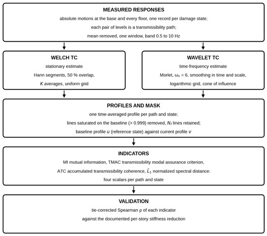
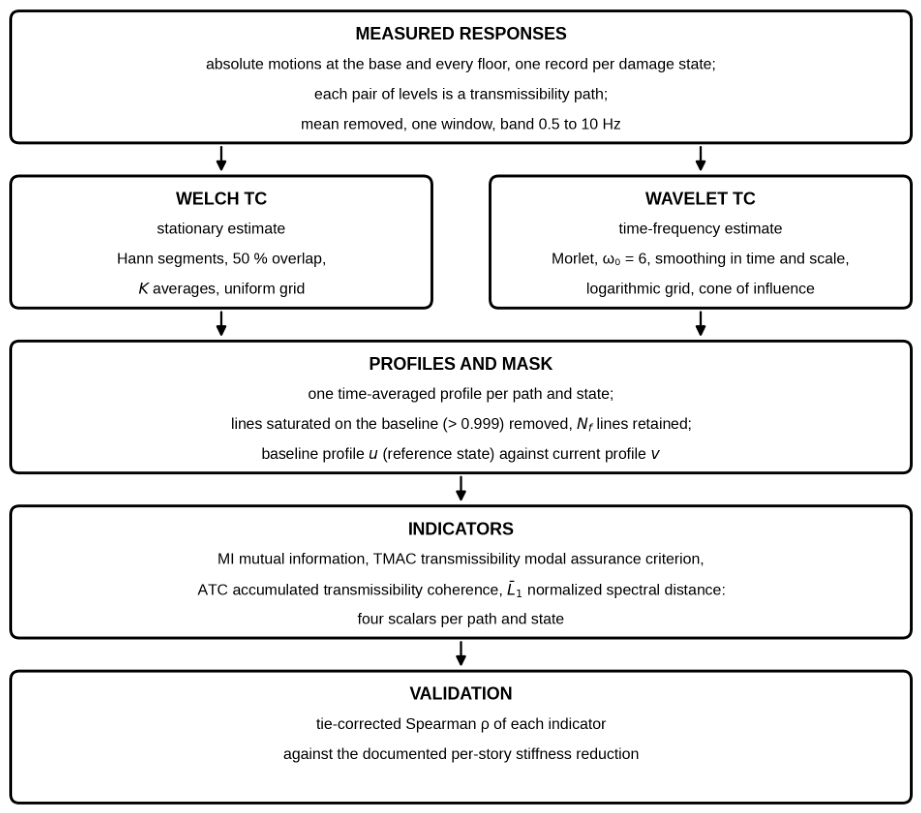
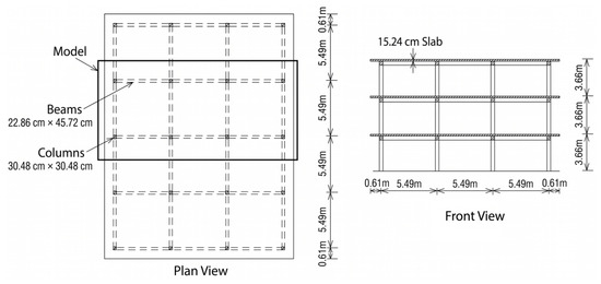
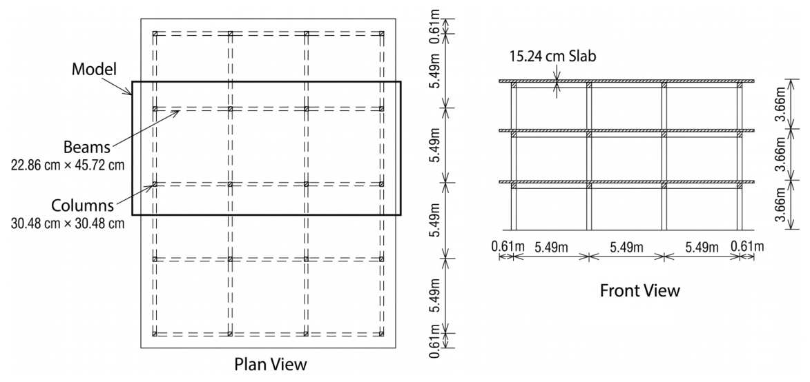
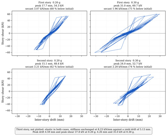
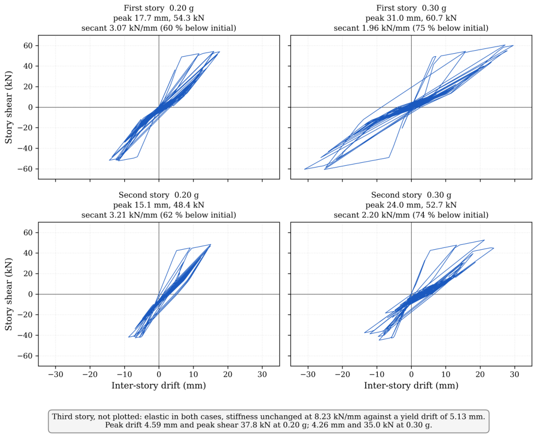
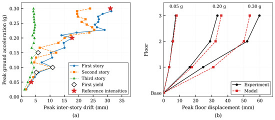
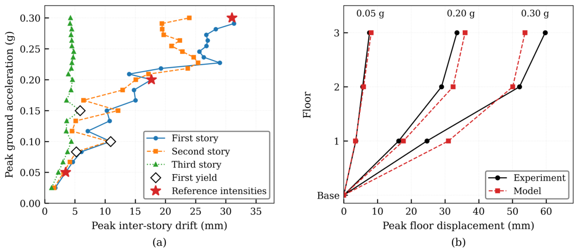
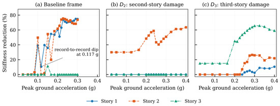
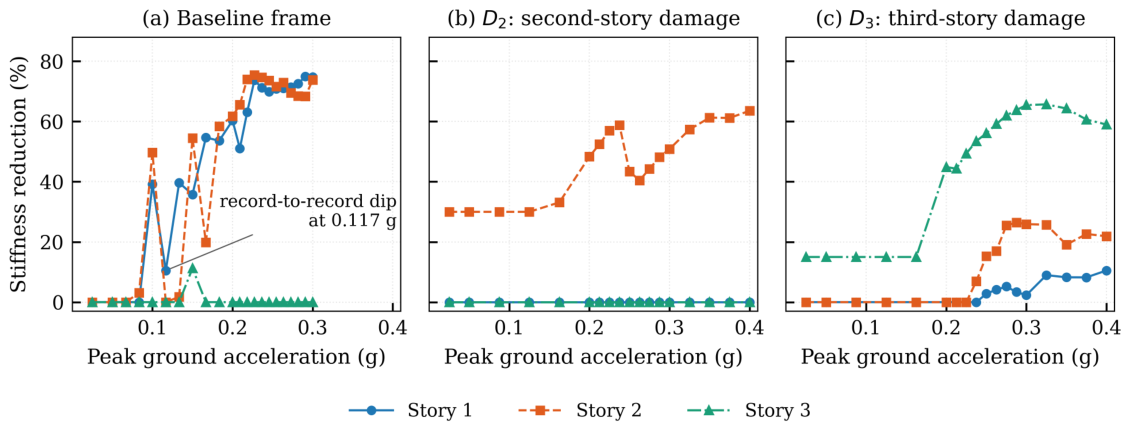
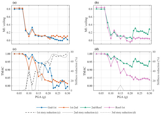
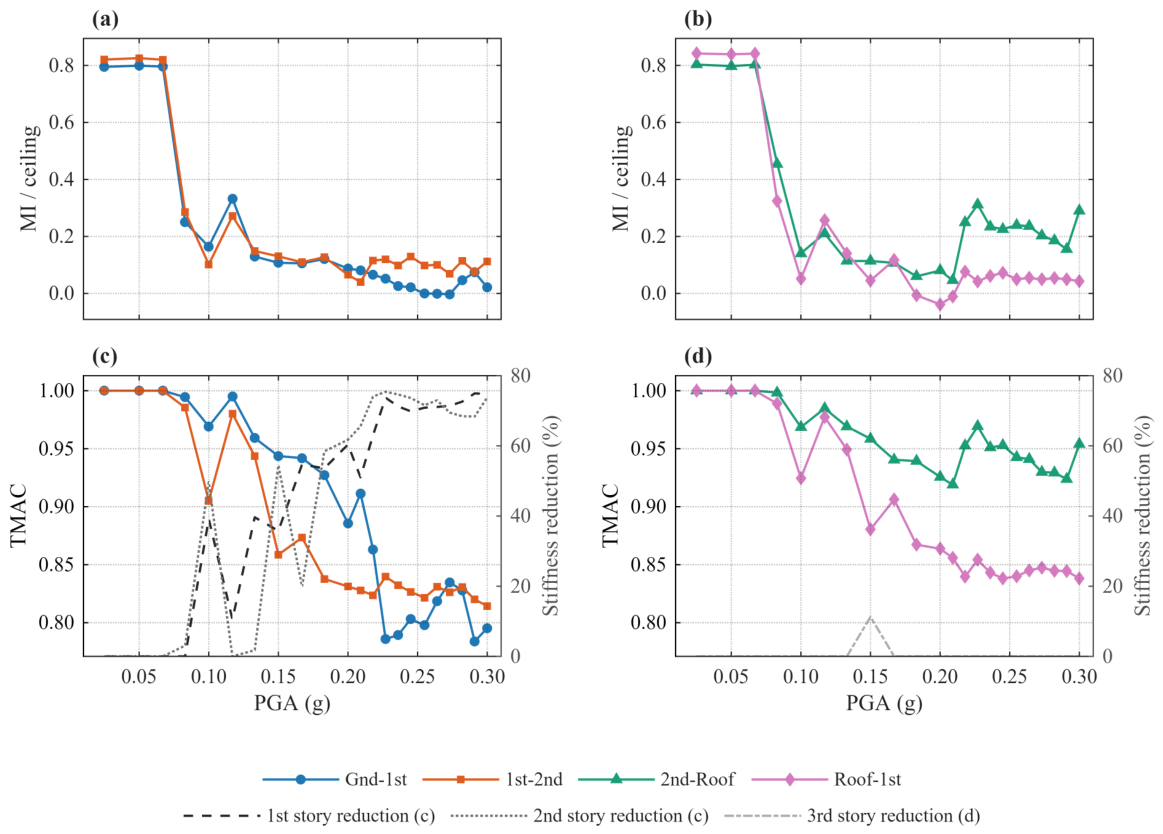
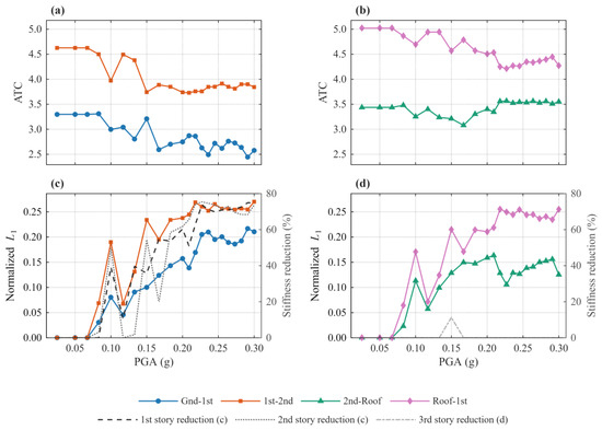
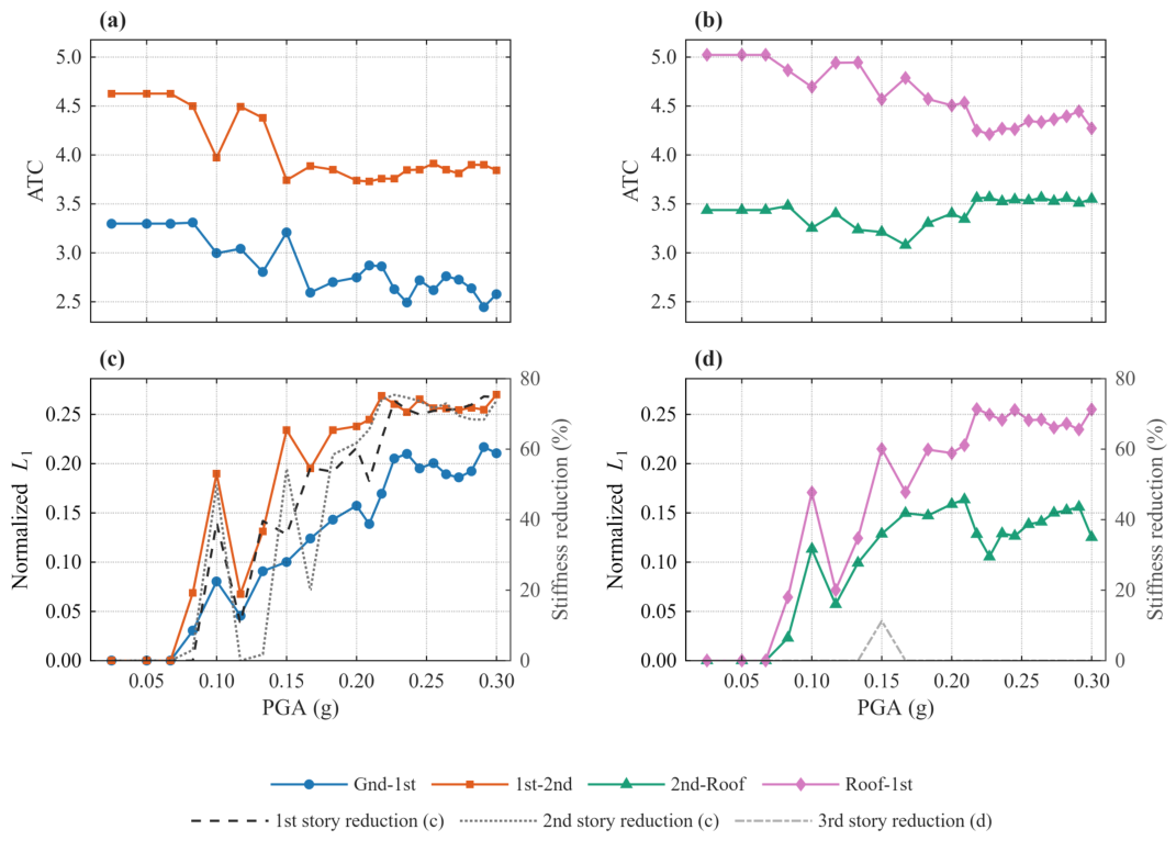
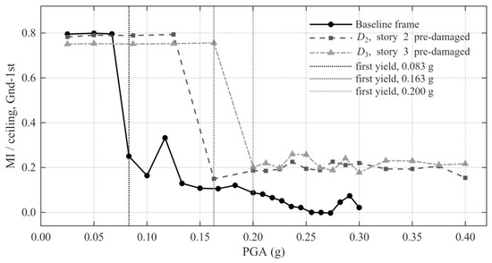
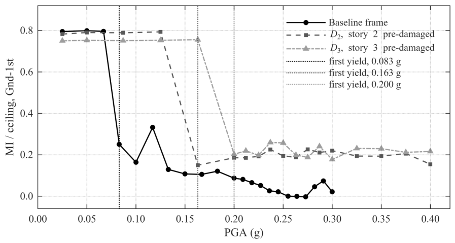
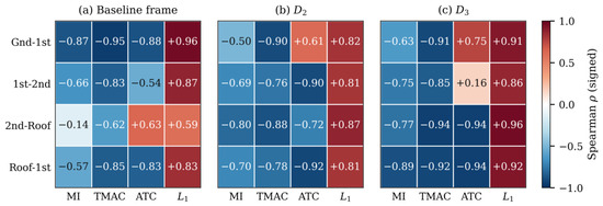
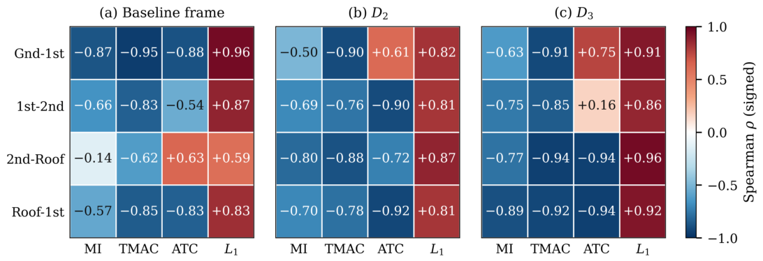
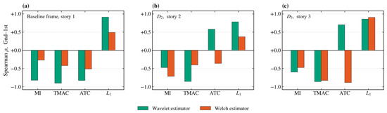
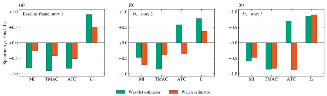
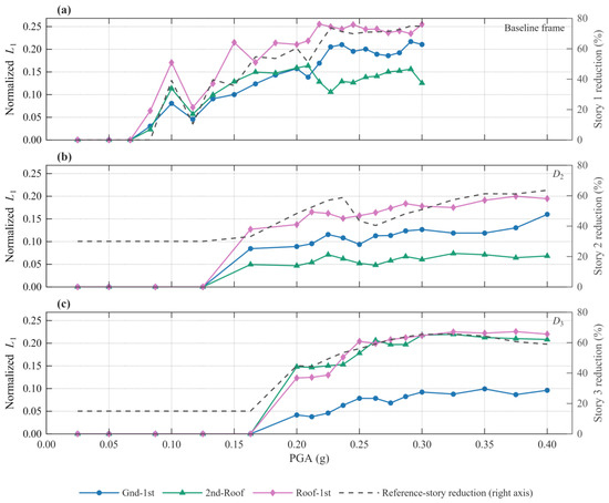
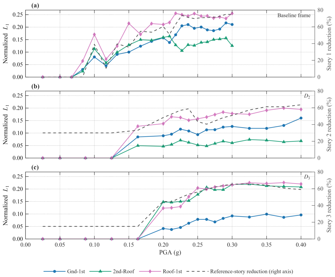
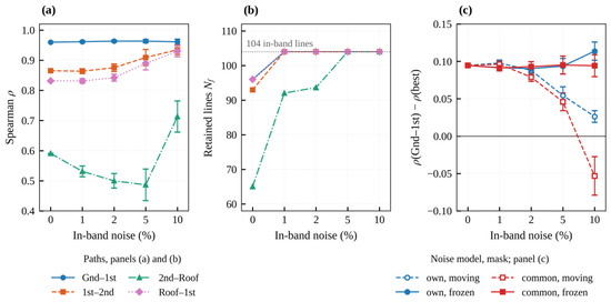
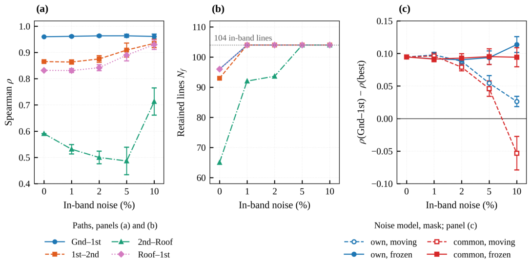
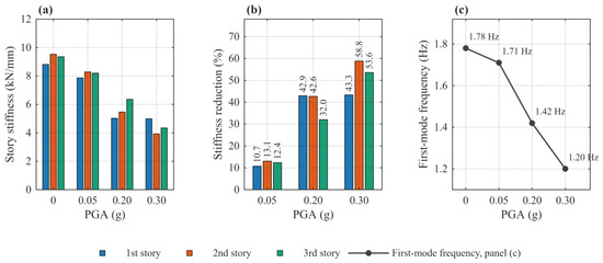
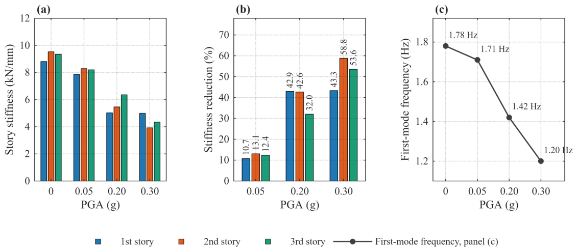
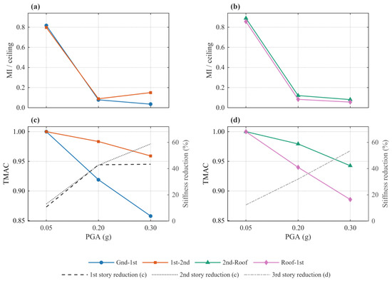
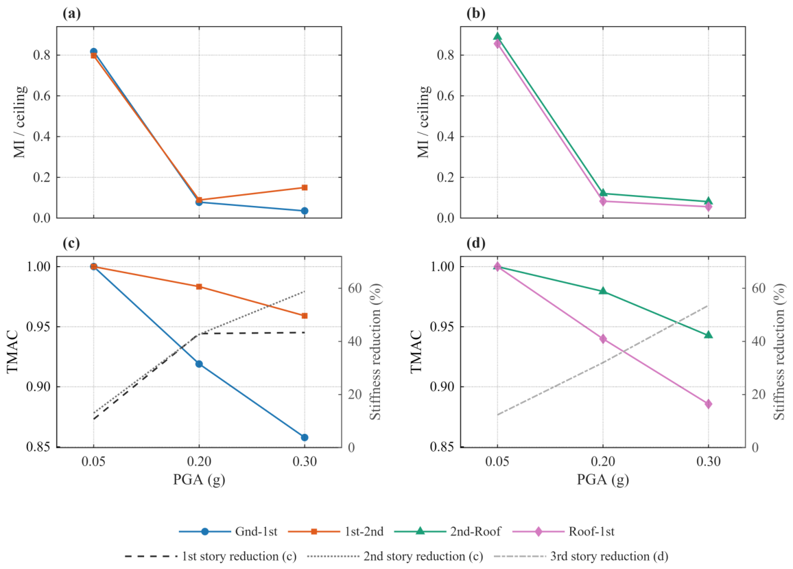
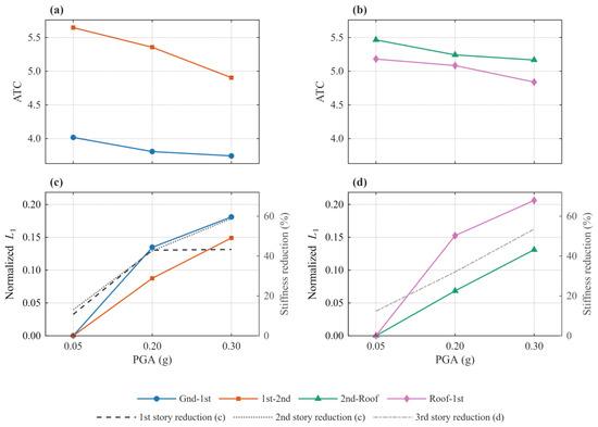
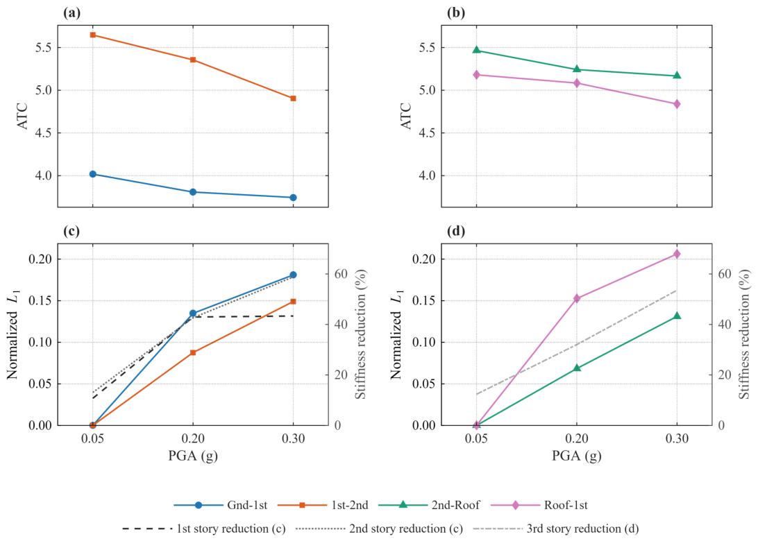
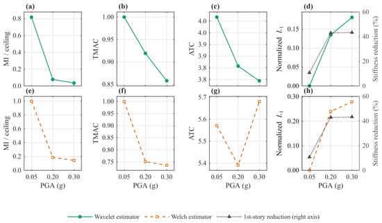
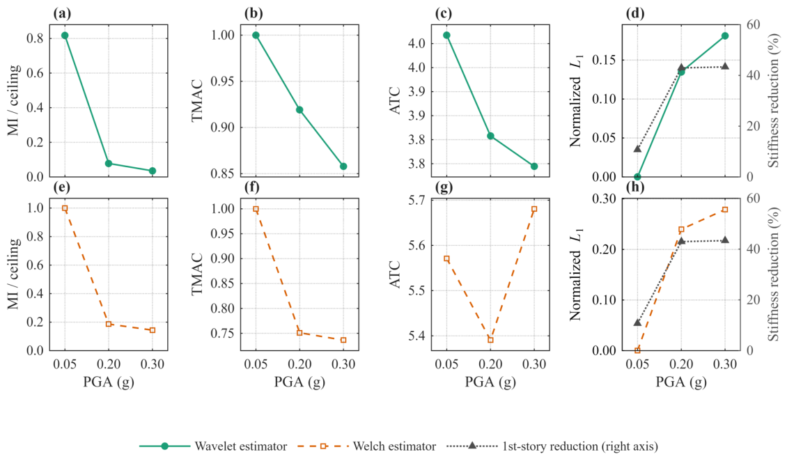
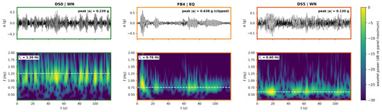
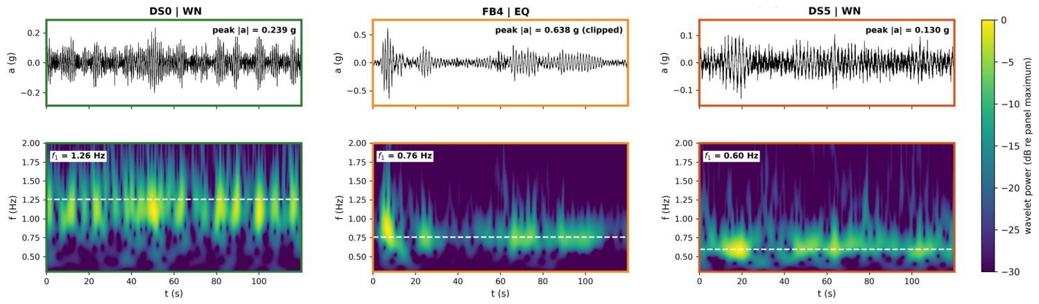
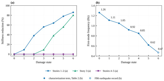
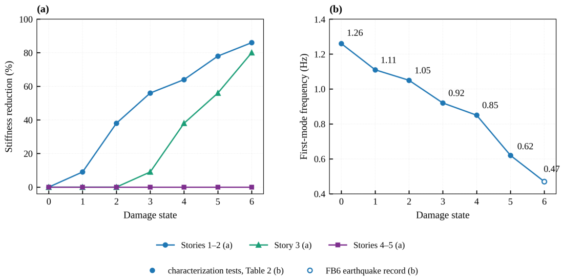
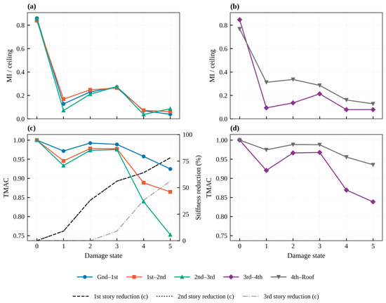
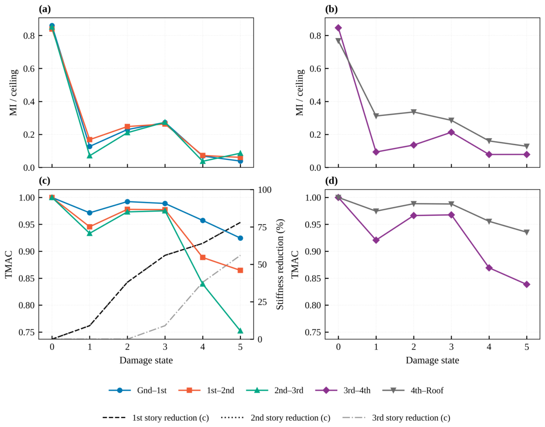
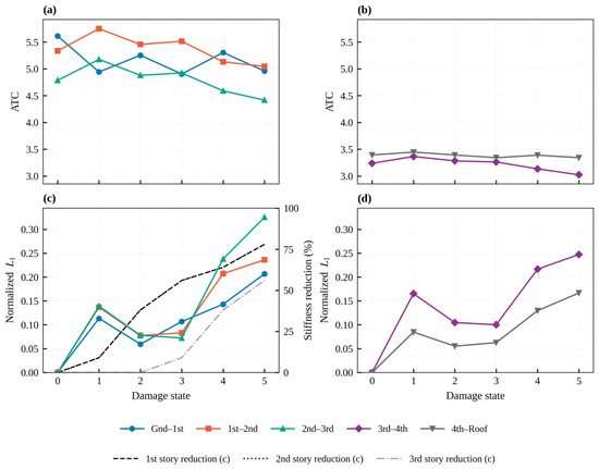
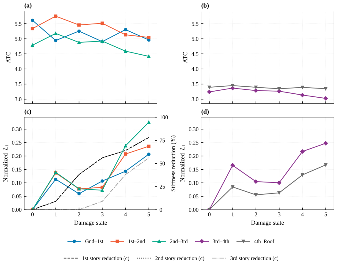
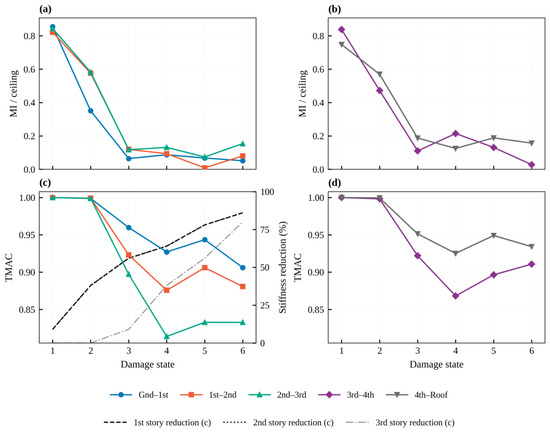
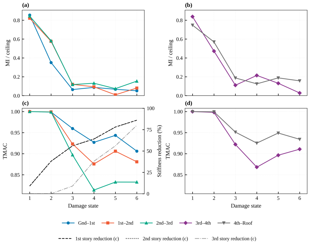
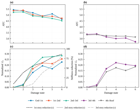
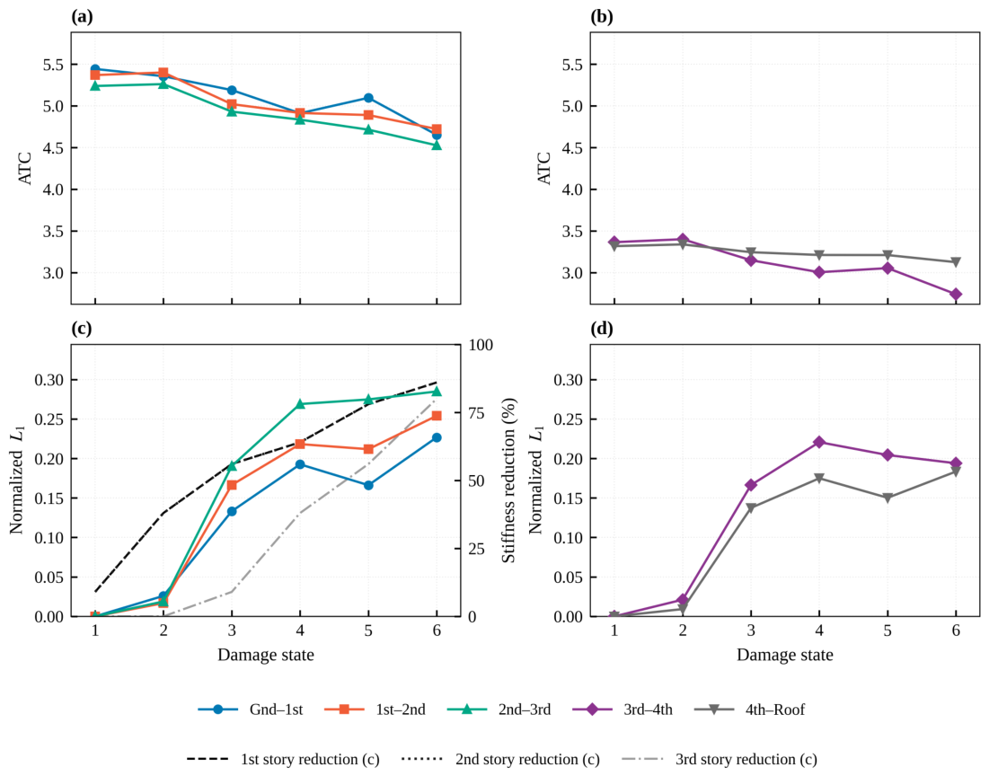
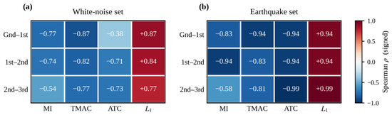
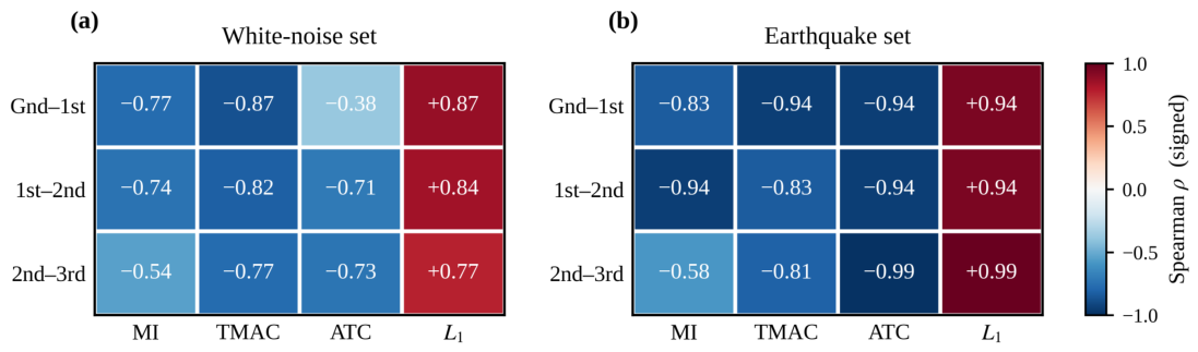
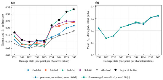
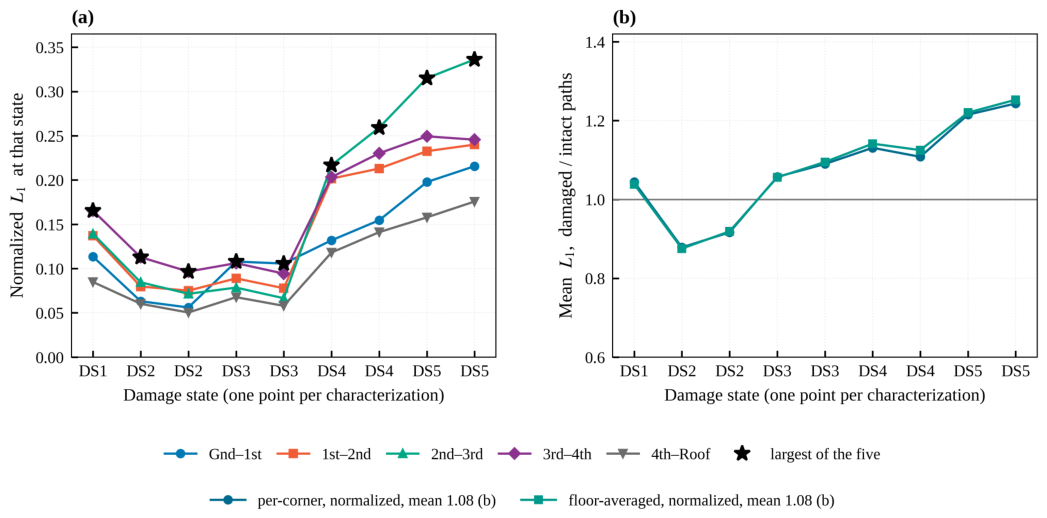
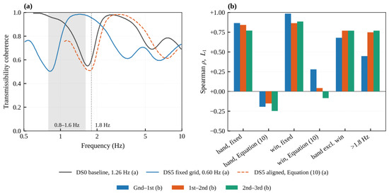
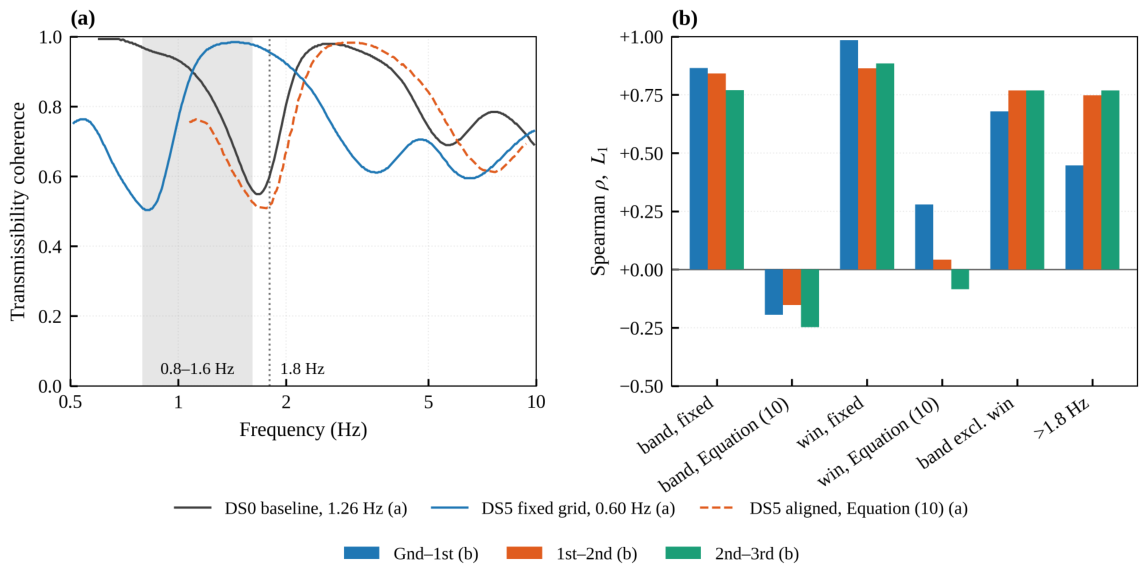
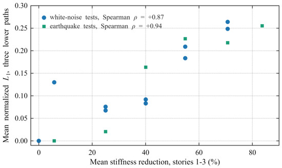
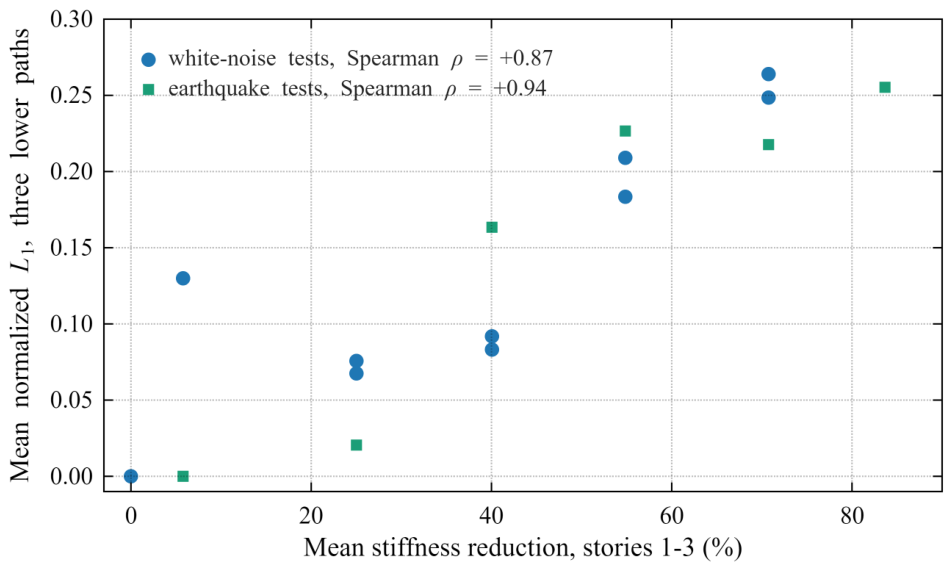

Disclaimer/Publisher’s Note: The statements, opinions and data contained in all publications are solely those of the individual author(s) and contributor(s) and not of MDPI and/or the editor(s). MDPI and/or the editor(s) disclaim responsibility for any injury to people or property resulting from any ideas, methods, instructions or products referred to in the content. |
© 2026 by the authors. Licensee MDPI, Basel, Switzerland. This article is an open access article distributed under the terms and conditions of the Creative Commons Attribution (CC BY) license.