Simulation-Based Decision Framework for Adaptive Construction Control in High-Rise Buildings: Structural Deformation and Correction Criteria

Abstract

High-rise construction requires both geometric setting-out and monitoring of structural movement. This paper presents a simulation-based decision framework for adaptive construction control. The numerical experiment is a synthetic uncertainty-propagation test: a prescribed storey-level deformation profile is treated as the input signal, while 500 Monte Carlo realisations represent repeated coordinate solutions affected by independent horizontal coordinate noise and a campaign-common reference-frame component. The Monte Carlo procedure does not simulate structural mechanics, raw Global Navigation Satellite System (GNSS) observables, satellite geometry or a full GNSS network adjustment; its purpose is to quantify how coordinate-level uncertainty affects threshold exceedance and decision-zone assignment. The same decision logic can be supplied by conventional geodetic techniques, provided that they deliver displacement estimates in a common reference frame; in a future field implementation, periodic GNSS ties could therefore be complemented by total-station and/or optical/laser-plummet observations. A four-zone decision rule combines the observed deformation magnitude with a transfer-risk indicator and is exercised on a synthetic 248 m, 62-storey benchmark geometry. Under the stated stress-test assumptions, the adopted correction model reduces the mean residual deformation on intervention storeys to approximately 1.1–3.3 mm. These values are outputs of the synthetic benchmark, not demonstrated field performance. The study therefore evaluates the internal consistency and uncertainty sensitivity of the decision logic and defines requirements for future observation-level and field validation.

1. Introduction

The increasing height and slenderness of modern buildings mean that surveying support for construction projects cannot be viewed merely as a procedure for transferring design axes and points between storeys. In construction practice, the geometric layout of a structure changes during construction under the influence of assembly loads, wind loads, temperature gradients, solar exposure of the façade, crane operations, uneven shortening of vertical elements (differences in stiffness, creep, shrinkage, concreting sequence), and local technological effects. From a surveyor’s perspective, this leads to a situation where the “current geometry of the structure” may deviate from the design geometry, and these discrepancies may increase systematically and in a height-dependent manner. The literature on the monitoring of tall structures indicates that the direct measurement of displacements and the dynamic/quasi-static response of tall structures is now a standard element of safety management and the validation of design assumptions [1,2,3,4,5]. At the same time, the traditional transfer of the vertical reference using optical/laser methods is still widely used in the construction of super-tall buildings; whilst effective, this method is sensitive to the accumulation of errors and to both transient and permanent structural movements. Zhang et al. [6] demonstrated, using a 438-metre-high building as an example, that horizontal displacements of the structure during construction (attributable, among other things, to wind, temperature, crane operations, and assembly loads) affect the accuracy of vertical reference transfer, and that static Global Navigation Satellite System (GNSS) measurements, after appropriate processing and referencing to a common datum, can be used to check/verify the results of laser plumb lines. Concurrently, research by Quesada-Olmo et al. [7] demonstrated the effectiveness of a local GNSS geodetic network for real-time monitoring on the Torre Espacio building, indicating the possibility of reducing the maximum error by approximately 40% thanks to a dedicated adjustment model. From the perspective of geodetic construction support, however, there is a lack of a coherently formulated decision-making model that would answer the question: when and how should deformations (deflections, drifts, differential shortening) result in a correction of the construction control network, and when is it sufficient to correct only the coordinates of the stakeout points? The aim of this paper is to fill this gap by combining a literature review with a decision-making model and a simulation study illustrating the consequences of various correction strategies.

1.1. Related Works

1.1.1. GNSS and Structural Health Monitoring (SHM) of Tall Structures

The monitoring of tall structures has evolved from Global Positioning System (GPS) and broader GNSS applications for identifying dynamic displacements in towers and tall buildings (including the Calgary Tower and wind-response studies) [8,9,10] to modern structural health monitoring (SHM) systems integrating acceleration, pressure, temperature and strain sensors, wireless systems and cloud platforms [2,4]. Reviews by Yi, Li and Gu and subsequent syntheses highlight the suitability of GNSS for measuring static and quasi-static displacement components that cannot be recovered reliably from accelerometers alone [4,5,11]. Tamura et al. and Park et al. demonstrated real-time kinematic GPS (RTK-GPS) for monitoring lateral and torsional wind-induced response [9,10]. Subsequent full-scale studies addressed super-tall structures during strong winds and typhoons and identified natural frequencies, damping and quasi-static responses to wind and temperature [12,13,14,15]. Quesada-Olmo et al. proposed a local GNSS geodetic network with a dedicated adjustment model for Torre Espacio (236 m), reporting a reduction in the maximum error and showing the value of GNSS for ongoing geometric monitoring [7]. Zhang et al. used static GNSS together with laser-plummet measurements to check the verticality of a 438 m building [6]. Choi et al. presented an automatic wireless sensor network (WSN) for monitoring vertical shortening in 66- and 72-storey buildings [16]. Differential axial shortening (DAS) and its compensation are further discussed in [17,18,19,20,21].

Recent international studies confirm that GNSS-based structural displacement monitoring continues to develop rapidly. Yu et al. applied GNSS-RTK denoising to displacement monitoring of a super-high-rise tower [22]; Yigit et al. evaluated real-time precise point positioning (PPP)/RTX for dynamic displacement and reported millimetre-level agreement after filtering in controlled tests [23]; Xiong et al. proposed improved denoising for GNSS-RTK monitoring of a super-high-rise building [24]; and Xiao et al. combined GNSS and accelerometer data for dynamic deformation analysis of super-high-rise buildings [25]. Collectively, these studies also show that achievable displacement accuracy is strongly dependent on the observation environment, processing strategy, multipath and noise treatment, and sensor configuration, which is especially important on an active high-rise construction site.

1.1.2. Deformation Mechanisms Relevant to Construction Surveying

From the perspective of engineering surveying, the key factors are deformations that alter the position of reference points for setting-out in the horizontal plane or change the geometric relationships between storeys. Based on the literature, at least five groups of phenomena can be distinguished: (i) transient and quasi-static wind deflections, (ii) thermal and solar-induced displacements, (iii) movements associated with erection loads and equipment operation (e.g., tower cranes), (iv) settlement and uneven displacement of the ground/foundations, and (v) shortening of vertical load-bearing elements, including differential shortening [6,7,12,13,14,15,16]. In GNSS/SHM studies of tall buildings, both dynamic responses (natural frequencies, vibration amplitudes) and quasi-static responses, which are particularly relevant for setting out, are reported. Su et al. demonstrated, using the example of a super-tall structure (Canton Tower), that temperature-induced quasi-static responses can be comparable to, and locally greater than, responses to strong winds/typhoons in the analysed scenario [13]. For a surveyor, this means that survey campaigns carried out at different times of day or under different temperature conditions may yield different coordinates for control points, even if there have been no changes to the construction methods on site. The shortening of vertical elements (and differences in shortening between the core wall and the perimeter columns) does not directly cause the entire structure to tilt in plan, but leads to local changes in storey geometry, relative displacements and the need for construction-stage compensation. Choi et al. report, in field data, maximum differential shortening of several millimetres on monitored pairs of elements, which is significant for the control of slabs, crane rails and cladding [16]. Studies on DAS (including Samarakkody et al.; Ruiz et al.; Kim et al.; and Elansary et al.) show that the scale of the phenomenon increases with height and depends on the material, stiffness, construction sequence, and rheological models [17,18,19,20,21]. In the context of geodetic reference transfer from storey to storey, the accumulation of systematic errors is particularly dangerous. If the current control point on storey n is determined from a point on storey n − 1, which has itself been displaced by deformation and measurement error, the error may accumulate with height. It is precisely this effect that provides the main justification for periodically “refreshing” the control network relative to an external reference system (e.g., via static GNSS) and for height-dependent decision-making procedures [6,7].

1.1.3. The Extent of Deformation in High-Rise Buildings During Construction and Its Significance for the Accuracy of the As-Built Surveys

No single universal range of high-rise-building deflection can be taken from the literature because the observed values depend on height, structural system, slenderness, construction stage, environmental conditions, averaging interval and measurement method. GNSS/SHM studies report horizontal movements from millimetres to centimetres, but the physical meaning depends on the time scale: instantaneous motion describes short-term vibration, quasi-static displacement describes slowly varying wind- or temperature-related response, and long-term drift describes persistent change that may be relevant to construction control [5,6,9,10,11,12,13,14,15]. For the 438 m building studied by Zhang et al. [6], horizontal displacements were commonly of the order of ±1 cm and the difference between GNSS and laser-plummet results after the authors’ vertical-deviation correction remained below ±2 cm. Their cited ±3 cm limit was a project/Chinese-standard requirement used in that case study; it is not adopted here as a universal tolerance and is not used to define the present T₁–T₃ or E₁–E₃ thresholds. Quesada-Olmo et al. reported short-term accuracies of approximately 0.2–3 cm for real-time GNSS solutions, depending on configuration and conditions [7]. These studies support a general methodological point: a correction decision should be based on processed measurements of known quality and on project-specific tolerances, not on a raw displacement value alone.

1.2. Research Gap and Rationale for the Proposed Approach

Despite the extensive literature on SHM and the numerous implementations of GNSS systems in monitoring, relatively few studies formulate an explicit decision layer that links deformation monitoring to ongoing geodetic construction control. The focus of this study is therefore the decision problem itself: how measured displacement and measurement quality can be converted into a transparent operational response. The framework contains four elements: (i) a construction control network tied to an external reference frame, (ii) a deformation-magnitude indicator and a transfer-risk indicator, (iii) separate actions for design-point correction and control-grid correction, and (iv) a four-zone escalation rule that can be tested under controlled uncertainty.

The contribution is intentionally limited to this decision layer. The numerical experiment uses a synthetic benchmark signal and coordinate-level uncertainty propagation; it is not a structural-response model and it is not a numerical validation of a complete multi-point GNSS network adjustment.

The main aim of this study is to formulate and test, in a controlled synthetic environment, the decision logic for adaptive updating of a high-rise construction control framework using deformation information expressed in a common geodetic reference frame. The experiment evaluates the internal consistency, sensitivity and stability of the decision rule when the same prescribed deformation signal is observed with repeated measurement uncertainty. It does not estimate the probability of a real structural deformation event. This aim has been broken down into four research questions:

• Which deformation mechanisms and typical response ranges of high-rise buildings, as reported in the literature, are relevant from the perspective of geodetic control network transfer and the setting out of structural elements?
• How should decision-making criteria be defined to determine whether a correction should be applied to the as-built control network or only to the coordinates of design points?
• What is the impact of applying adaptive corrections on the residual positional errors of stakeout points on subsequent storeys?
• How can the decision-making process and the effects of corrections be illustrated in a form that is clear for surveying practice (limit plots, storey sketches, elevation profiles)?

2. Materials and Methods

2.1. Dynamic Construction Control with Periodic GNSS Ties

A dynamic construction control network is defined here as a set of working control points whose coordinates may be updated when a persistent displacement becomes operationally significant. GNSS is one possible means of tying selected points to a stable external datum, but it is not the only surveying technique capable of supporting the workflow. The field system may combine: (1) external GNSS reference points/stations; (2) control points on the structure observed by GNSS and/or conventional total stations, optical or laser plummets; (3) geometric relationships from the Building Information Modelling (BIM) or computer-aided design (CAD) model; and (4) project-specific technical criteria. Periodic GNSS sessions are particularly useful for an independent tie to an external reference frame, whereas total stations and plummets can provide precise relative geometry and vertical transfer where satellite visibility is restricted. The decision layer developed in this paper is measurement-technique-agnostic: it requires a displacement estimate and its quality measure in a common datum, regardless of whether those quantities originate from GNSS, conventional geodetic measurements, or a hybrid solution.

Scope of the present numerical model: The operational concept contains external reference stations, a working floor grid and a quality-control step, but the numerical experiment reported here is not a least-squares simulation of a complete geodetic network. The five floor points define the intended layout and are used for plan-view illustrations; the Monte Carlo model assigns one resultant horizontal translation vector to each storey. The model represents GNSS at the post-processed coordinate-solution level through horizontal coordinate noise and a campaign-common reference-frame term. It does not generate pseudorange/carrier-phase observations, satellite geometry, ambiguity resolution, baseline correlations or point-specific covariance. Consequently, the numerical results test the stability of the decision rule, not the performance of a complete GNSS adjustment. The same decision rule could be coupled to a rigorously adjusted total-station or hybrid network in field implementation.

2.2. Research Methodology

2.2.1. Research Assumptions and Procedures

The study is methodological and uses a synthetic stress-test benchmark rather than a model of a specific construction project. A hypothetical 248 m geometry with 62 storeys (4.0 m per storey) and a 36 × 24 m floor plan is used only to provide a height grid and an illustrative plan configuration. The storey-level horizontal deformation profile is prescribed as an input signal; it is not calculated from loads, stiffness, material properties or a finite-element model. The benchmark combines a gradual height-dependent component with a localised upper-storey disturbance so that the decision rule is exercised under both progressive and local threshold crossings. Measurement uncertainty is introduced separately through the coordinate-observation model in Section 2.2.2. This separation between prescribed signal, measurement uncertainty and decision rule is fundamental to the interpretation of the numerical experiment.

Meaning of the Monte Carlo experiment: In this study, one Monte Carlo realisation represents one hypothetical repetition of the coordinate-determination process for the same fixed deformation profile. The structural input signal is not re-generated between realisations. For each realisation j, one x- and one y-component of the reference-frame bias are drawn and applied to all storeys, while independent x- and y-coordinate noise terms are drawn separately for every storey. These stochastic terms are added to the prescribed displacement components, after which the observed deformation magnitude, the transfer-risk indicator and the S_I–S_IV decision zone are calculated. Repeating this process 500 times produces empirical distributions, threshold-exceedance probabilities and zone-assignment probabilities. Thus, the Monte Carlo analysis propagates measurement uncertainty through the decision rule; it does not simulate the physics of the building.

Relation of the assumptions to field conditions. The horizontal coordinate-noise parameter ${\sigma }_{GNSS}$ = 2.5 mm is intentionally a favourable engineering scenario rather than a guaranteed performance specification. Recent GNSS-RTK/PPP and multisensor studies report performance ranging from a few millimetres after filtering under controlled or favourable conditions to centimetre-level scatter under less favourable configurations [22,23,24,25]. A high-rise construction site can additionally introduce changing satellite visibility, multipath from façades and steel, signal masking by cranes, antenna centring or monument instability, and time-varying atmospheric and reference-station effects. These mechanisms are not simulated separately here; their combined influence is represented only through the adopted uncertainty parameters and the sensitivity analysis. The simulated accuracy should therefore be read as a test of decision logic, not as a prediction of field GNSS performance.

Control-point configuration: The five points (four corners plus the centre) are used only to illustrate the intended floor layout. The numerical state variable is a single horizontal translation assigned to each storey, so all five schematic points share the same storey displacement. Consequently, this experiment does not assess network-geometry effects, floor rotation, shear, local point deformation or optimum network density. Those effects require a point-specific observation model and a full network adjustment. In a field implementation, three well-distributed non-collinear points constitute a practical minimum for an internally checkable planar transformation, while four or more points provide useful redundancy for gross-error detection; denser layouts may support affine or local-deformation diagnosis at the cost of additional observations.

2.2.2. Observation Model, Uncertainty Representation and Decision Metrics

The numerical model starts from a storey-level horizontal displacement vector expressed in the external construction reference frame:

$$d_i=\left[\begin{array}{c}{d}_{x,i}\\ d_{y,i}\end{array}\right]$$

(1)

where $d_i$ is the horizontal displacement vector for storey i and $\left|d_i\right|$ is its Euclidean magnitude. In a future field implementation, $d_i$ would be obtained by differencing adjusted coordinates between the current campaign and a chosen reference epoch after datum control and quality testing. In the present simulation, $d_i$ is generated from the benchmark deformation model rather than estimated from raw GNSS observations.

$$‖d_i‖=\left|d_i\right|=\sqrt{d_{x,i}^2+d_{y,i}^2}$$

(2)

To support an operational decision, a second quantity $e_i$ is introduced. It is a transfer-risk indicator, expressed in millimetres, that combines the coordinate uncertainty allowance, height-dependent propagation and the observed deformation magnitude:

$$e_i=f\left(z_i,‖d_i‖\right)$$

(3)

The function $f$ is not calibrated from field data in this simulation. “Calibration” denotes a future empirical estimation of the coefficients $k_z$ and $k_d$, and, separately, of the intervention thresholds, from repeated construction campaigns. The calibration target would be the residual difference between coordinates/setting-out results predicted by the working control and independently verified check measurements. Coefficients would be selected so that the indicator e predicts the risk of consuming the available setting-out tolerance without being interpreted as a statistical standard deviation. In the present demonstrative study, kz, kd and all thresholds are scenario parameters listed in Table 1.

$$M_{1,i}=‖d_i‖ M_{2,i}=e_i M_{3,i}={\sigma }_i M_{4,i}=z_i$$

(4)

The symbols $M_{1,i}-M_{5,i}$ are bookkeeping variables used to separate the information entering the decision: $M_{1,i}$ is the observed deformation magnitude, $M_{2,i}$ is the transfer-risk indicator, $M_{3,i}$ is the standard uncertainty of the storey coordinate solution, $M_{4,i}$ is the storey height, and $M_{5,i}$ is the set of intervention thresholds. They are not five independent sensors or five measured deformation components. Only $M_{1,i}$ and $M_{2,i}$ enter the two-dimensional zone classifier directly; $M_{3,i}$ and $M_{4,i}$ contribute through $e_i$, while $M_{5,i}$ defines the decision boundaries.

$$M_{5,i}=\left(T_1,T_2,T_3\right) T_1<T_2<T_3$$

(5)

Table 1. Synthetic benchmark, uncertainty-propagation and decision parameters used in the study.

Symbol/Parameter	Value (in the Simulation)	Meaning
H	248 m	Building height (reference object)
N	62	Number of storeys (height increment Δz = H/N = 4.0 m)
Projection	36 × 24 m	Floor plan dimensions (regular model)
Control points	5 (illustrative geometry)	4 corners + centre point O; one common storey translation is simulated, not five independent point adjustments
Model $\left|d\right|\left(z\right)$	Equation (8)	Power-law baseline + deterministic localised bell-shaped anomaly; synthetic stress-test input, not a structural constitutive model
a	55 mm	Amplitude of the global height-dependent component at z = H
p	1.6	Exponent of deviation increase with height
A, $z_0$, ${\sigma }_z$	20 mm, 210 m, 18 m	Localised-anomaly amplitude, centre height and vertical spread
Direction $\theta \left(z\right)$	$\theta \left(0\right)$ = 20°; $\theta \left(H\right)$ = 45°	Deterministic azimuth interpolation used only to obtain x–y components for visualisation
${\sigma }_{GNSS}$	2.5 mm	Scenario standard deviation of independent horizontal Global Navigation Satellite System (GNSS) coordinate noise (processed solution + centring/stabilisation)
${\sigma }_{ref}$	2.0 mm	Scenario standard deviation of a two-dimensional reference-frame bias drawn once per Monte Carlo campaign
$e\left(z,\left|d\right|\right)$	Equation (16)	Transfer-risk indicator [mm]; not a statistical error or standard deviation
$k_z$	10 µm/m = 0.01 mm/m	Height coefficient in the transfer-risk indicator
$k_d$	0.10	Dimensionless deformation coefficient in the transfer-risk indicator
Monte Carlo	500 realisations	Distribution and decision-stability analysis
$\left|d\right|$ thresholds	T1 = 10 mm; T2 = 20 mm; T3 = 40 mm	Internal intervention thresholds for deformation magnitude |d|
e thresholds	E1 = 4 mm; E2 = 7 mm; E3 = 12 mm	Internal intervention thresholds for the transfer-risk indicator e

The threshold set $M_{5,i}$ contains T₁–T₃ for deformation magnitude and E₁–E₃ for the transfer-risk indicator. These values are internal intervention levels for the simulation, not universal construction tolerances.

Four decision zones have been adopted:

S_I—no correction (continuation of monitoring);

S_II—correction of design points (without redefining the grid);

S_III—correction of the construction grid on the storey;

S_IV—correction of the grid and alarm/re-analysis (re-measurements, verification of causes, consultation with the designer/site manager).

The zones are defined on the plane

$$\left(‖d_i‖,e_i\right)$$

(6)

The corresponding decision plane is presented in the Results section.

The simulation tests whether the S_I–S_IV assignment remains stable when the same structural signal is observed with realistic coordinate-level disturbances. GNSS enters the analysis through two explicit stochastic terms: independent horizontal coordinate noise with standard deviation ${\sigma }_{GNSS}$ and a two-dimensional reference-frame bias with standard deviation ${\sigma }_{ref}$ that is common to all storeys within one Monte Carlo campaign. This is a simplified model of a processed GNSS coordinate solution; it is intentionally less detailed than an observation-level GNSS network adjustment.

$$\mathcal{D}:\left({\left|d\right|}_{i,obs}, e_i\right)\to S_i\in \left\{S_I,S_{II},S_{III},S_{IV}\right\}$$

(7)

Benchmark geometry and elevation grid: The synthetic geometry has H = 248 m, N = 62 storeys and Δz = 4.0 m, so z_i = iΔz. The plan-view sketch contains four corner points and one central point. Because a single rigid translation is assigned to each storey, the numerical experiment evaluates only translation-based decision logic. Rotation, shear, point-specific deformation and the influence of network geometry are outside the scope of this benchmark and must be addressed in a future point-specific network model.

Deterministic benchmark deformation: The “true” deformation magnitude is constructed from a smooth height-dependent baseline and one localised anomaly:

$${\left|d\right|}_{true}\left(z\right)=a{\left({\displaystyle \frac{z}{H}}\right)}^p+A \exp \left(- {\displaystyle \frac{{\left(z-z_0\right)}^2}{2{\sigma }_z^2}}\right)$$

(8)

Equation (8) defines a synthetic benchmark signal, not a structural constitutive law and not a probabilistic deformation model. The first term, $a{\left(z/H\right)}^p$, provides a smooth global component that increases with height. The second, $A \exp \left(- {\left(z-z_0\right)}^2/2{\sigma }_z^2\right)$, is a deterministic localised bell-shaped basis function. It is added so that the decision rule is tested not only during a gradual approach to the thresholds but also in the presence of a localised upper-storey excursion. Although this exponential term has the mathematical shape of a Gaussian kernel, it is not a Gaussian probability density and carries no probabilistic interpretation: A controls the peak amplitude, $z_i$ its location and ${\sigma }_z$ its vertical spread. The parameter values are selected to make the synthetic signal traverse several decision zones and are not calibrated to a particular building. Consequently, Equation (8) is suitable only as a controlled stress-test input; field application would require replacing it with measured deformation histories or a structurally validated prediction model.

$$\theta \left(z\right)={\theta }_0+gz,\theta \left(z\right)=20°,g=\left(45°-20°\right)/H$$

(9)

For each storey, the “true” displacement vector is expressed as:

$$d_{x,i}^{true}={\left|d\right|}_{true}(z_i) \mathrm{c}\mathrm{o}\mathrm{s}\theta (z_i) d_{y,i}^{true}={\left|d\right|}_{true}(z_i) \mathrm{s}\mathrm{i}\mathrm{n}\theta (z_i)$$

(10)

Observation model and disturbance distributions: Each Monte Carlo campaign j represents a repeated realisation of the processed horizontal coordinate solution. For each storey, independent coordinate noise is drawn for the x and y components:

$${\epsilon }_{x,i}^{\left(j\right)}~\mathcal{N}(0,{\sigma }_{GNSS}^2),{\epsilon }_{y,i}^{\left(j\right)}~\mathcal{N}(0,{\sigma }_{GNSS}^2)$$

(11)

The parameter ${\sigma }_{GNSS}=2.5 \mathrm{m}\mathrm{m}$ is a favourable scenario value for the horizontal coordinate noise of a processed static/rapid-static solution together with centring/stabilisation effects; it is not claimed as a universal site accuracy. The external reference tie is represented separately by ${\sigma }_{ref}=2.0 \mathrm{m}\mathrm{m}$. The combined standard uncertainty used as a scalar allowance in the decision indicator is

$$u=\sqrt{{\sigma }_{GNSS}^2+{\sigma }_{ref}^2}$$

(12)

A common reference-frame component is then drawn once per campaign and applied to all storeys. This creates a simple within-campaign correlation.

$$b_{x,ref}^{\left(j\right)} ~ \mathcal{N}\left(0,{\sigma }_{ref}^2\right),b_{y,ref}^{\left(j\right)} ~ \mathcal{N}\left(0,{\sigma }_{ref}^2\right),{\eta }_{x,i}^{\left(j\right)}={\epsilon }_{x,i}^{\left(j\right)}+b_{x,ref}^{\left(j\right)},{\eta }_{y,i}^{\left(j\right)}={\epsilon }_{y,i}^{\left(j\right)}+b_{y,ref}^{\left(j\right)}$$

(13)

Only uncertainty in the horizontal coordinate components and in the common reference-frame tie is included in the present stochastic model. No separate random azimuth perturbation is introduced because the S_I–S_IV classifier depends on the resultant deformation magnitude |d| and the transfer-risk indicator e, not on azimuth. Directional uncertainty becomes relevant when a point-specific model estimates rotation, shear or direction-dependent deformation and should then be introduced through the corresponding covariance model.

The observed storey displacement components are therefore

$$d_{x,i}^{\left(j\right)}=d_{x,i}^{true}+{\eta }_{x,i}^{\left(j\right)},d_{y,i}^{\left(j\right)}=d_{y,i}^{true}+{\eta }_{y,i}^{\left(j\right)}$$

(14)

and the corresponding observed deformation magnitude is

$${\left|d\right|}_{i,obs}^{\left(j\right)}=\sqrt{{\left(d_{x,i}^{\left(j\right)}\right)}^2+{\left(d_{y,i}^{\left(j\right)}\right)}^2}$$

(15)

Transfer-risk indicator: The quantity $e_i^{\left(j\right)}$ is not treated as an observed error or as a standard deviation. It is an operational transfer-risk indicator that combines the uncertainty of the coordinate solution with height-dependent transfer effects and the deformation magnitude. The indicator is therefore used only for decision classification and should be calibrated against independent check measurements and project-specific tolerances before field application.

$$e_i^{\left(j\right)}=u+k_z{z}_i+k_d{\left|d\right|}_{i,obs}^{\left(j\right)}$$

(16)

In Equation (16), u is a combined standard-uncertainty allowance, $k_z{z}_i$ is an engineering term representing increasing difficulty of reference transfer with height, and $k_d{\left|d\right|}_{i,obs}^{\left(j\right)}$ is a dimensionally consistent deformation-related allowance. Thus, e is not “the error”; it is a conservative scalar indicator used only to trigger a response. For each storey and Monte Carlo campaign, the pair (${\left|d\right|}_{i,obs }$, $e_{\mathrm{i}}$) is classified using T₁–T₃ and E₁–E₃. The maximum-risk principle is applied: if the two indicators imply different zones, the higher zone is selected.

N_MC = 500 Monte Carlo uncertainty realisations were performed for the same prescribed deformation profile. The number 500 was chosen as a practical compromise for the demonstrative sensitivity study; the reported statistics are empirical summaries of the uncertainty-propagation experiment, not frequencies of structural events. The following output metrics were reported:

• the distributions of ${\left|d\right|}_{i,obs}$ and $e_{\mathrm{i}}$ (e.g., the median and the P₅–P₉₅ percentiles).
• the probabilities of exceeding the thresholds P($\left|d\right|$ > T_k) and P($e$ > E_k).
• the stability of zone classification for each storey:

$$P_i\left(S_k\right)={\displaystyle \frac{1}{N_{MC}}}{\displaystyle {\sum }_{j=1}^{N_{MC}}}1\left\{S_i^{\left(j\right)}=S_k\right\} k\in \left\{I,II,III,IV\right\}$$

(17)

where 1{A} is the indicator function: it equals 1 when condition A is true and 0 otherwise. The overall proportion of storeys assigned to each zone is then calculated from all Monte Carlo realisations and storeys.

$$P\left(S_k\right)={\displaystyle \frac{1}{N_{MC}N}}{\displaystyle {\sum }_{j=1}^{N_{MC}}}{\displaystyle {\sum }_{i=1}^N}1\left\{S_i^{\left(j\right)}=S_k\right\}$$

(18)

In addition, the sensitivity of the decision boundaries to the parameters ${\sigma }_{GNSS}$, $k_z$ and $k_d$ was assessed through a series of simulations for different values of these parameters, and by analysing changes in the proportion of storeys in zones S_III–S_IV and shifts in the heights at which threshold exceedances become likely. The sensitivity study was also extended to the deterministic deformation-profile parameters a, p and A. A local one-at-a-time analysis was performed by changing each parameter by −20% and +20% around its baseline value while keeping the other parameters fixed. Each case used N_MC = 500 Monte Carlo realisations and the same random-number stream (common random numbers) so that differences in the decision-zone statistics are attributable to the profile parameter rather than to a different noise realisation. The evaluated outputs were the mean proportion of storeys assigned to Zones III–IV and the heights at which the probability of assignment to Zones III–IV and Zone IV first reached 0.5. The complete Monte Carlo uncertainty-propagation workflow is summarised in Algorithm 1.

Algorithm 1. Monte Carlo uncertainty-propagation procedure for SI–SIV decision stability

1. Set the synthetic deformation-profile parameters, uncertainty parameters and decision thresholds (Table 1), together with H, N and Δz; calculate u once from Equation (12). 2. For j = 1, …, NMC do (one hypothetical repetition of the coordinate-determination process): 2.1 Generate the independent campaign-common x- and y-reference-frame components according to Equation (13); keep these two values fixed for all storeys in realisation j. 2.2 For each storey i = 1, …, N: (a) Calculate the prescribed deformation magnitude from Equation (8) and the azimuth from Equation (9), and obtain the corresponding deterministic x- and y-components from Equation (10). (b) Generate independent x- and y-coordinate noise components according to Equation (11), and combine them with the campaign-common reference-frame components according to Equation (13). (c) Calculate the observed x- and y-displacement components from Equation (14), and the resultant observed deformation magnitude from Equation (15). (d) Calculate the transfer-risk indicator $e_i^{\left(j\right)}$ from Equation (16), using the value of u calculated once in Step 1. (e) Determine the zone from the deformation thresholds and independently from the transfer-risk thresholds; assign the higher of the two ordered zone levels I < II < III < IV (maximum-risk principle). 3. After all NMC realisations, calculate the empirical distribution of ${\left|d\right|}_{obs}$ and e, threshold-exceedance probabilities, and the probability of assignment to each SI–SIV zone for every storey.

2.2.3. Multi-Stage Procedure

Stage 1: Systematic monitoring of the same structural points. On successive storeys, a repeatable set of control points (or homologous points) is observed, enabling the estimation of the deformation trend as a function of height and time. The minimum variant includes working control points, whilst the extended variant includes additional points on the perimeter/core and SHM sensors.

Stage 2: Network adjustment and quality control. For a static GNSS campaign, network adjustment, analysis, coarse error tests and an assessment of coordinate uncertainty are carried out. If the quality of the solution is insufficient, the campaign should not initiate geometric corrections (observations must first be repeated or supplemented). Proposed field implementation strategy. A realistic pilot implementation would use a hybrid architecture. Periodic static or rapid-static GNSS sessions would tie selected storey or roof control points to stable external reference stations, while total-station observations and/or laser plummets would support floor-level geometric transfer; network RTK could be used as a rapid screening or verification tool when site conditions permit. Campaigns may be scheduled every few storeys (for example, every 3–5 storeys in an illustrative workflow), after significant loading or meteorological events, and whenever decision metrics approach a threshold. Acceptance should be based on ambiguity status, residuals and covariance from adjustment, repeated-session agreement, redundancy/outlier tests, and an independent check by total station, laser plummet, inclinometer or SHM sensors. Exact session duration and cadence must be calibrated to the site rather than prescribed by this simulation.

Stage 3: Deformation analysis and classification into decision zones. Displacement vectors of control points, elevation trends and any local anomalies are determined, and the impact on the transfer error of the control network/stakeout points is estimated. At this stage, storeys (or groups of storeys) are assigned to zones I–IV.

Persistence test before geometric correction: A single displacement epoch should not automatically redefine the construction grid. Wind- and temperature-induced elastic motion must first be separated from persistent settlement or quasi-static drift using repeated observations, short-term averaging, meteorological and loading records and, where available, tilt, temperature or other SHM data. A grid correction should be applied only to a persistent or operationally relevant quasi-static component referenced to the intended design geometry. A transient reversible response should trigger repeated monitoring rather than immediate grid redefinition, while differential shortening and other local deformations should be handled as a separate technological compensation layer.

Stage 4: Implementation of corrections. In Zone II, the coordinates of the design points are modified (correction staking-out), whilst retaining the existing working control network. In Zone III, the coordinates of the construction control points on each storey are updated, and the updated control network is then used to determine the design points. In Zone IV, an additional emergency procedure is initiated: more frequent monitoring, confirmation of results using alternative techniques (e.g., total station surveying, laser plumb line, inclinometry) and verification of causes.

Stage 5: Archiving and empirical calibration. All observation epochs, adjusted coordinates, independent check measurements, decisions and as-built residuals should be archived. In a field implementation, $k_z$ and $k_d$ would be estimated against independently verified transfer/setting-out residuals, while T₁–T₃ and E₁–E₃ would be tuned to project tolerances and an agreed false-alarm/omission-risk policy. No such field calibration is performed in the present simulation; the numerical values in Table 1 remain demonstrative scenario parameters.

The numerical study is a synthetic stress test of the decision logic. The deformation-profile parameters, thresholds and transfer-risk coefficients are scenario inputs selected to exercise the classifier over all four zones; they are not calibrated parameters of a specific high-rise building. Accordingly, the numbers of storeys in individual zones and the residual reductions reported below are benchmark outputs, not normative recommendations or expected field values. Field implementation requires project-specific calibration using design tolerances, instrument performance, control-network geometry, environmental conditions, construction sequence and independent verification measurements.

Relation of the adopted thresholds to construction and surveying tolerances. ISO 4463-1:1989 [26] addresses building setting-out, including the transfer of reference lines between floors, and gives permissible measuring deviations and acceptance criteria for the surveying process, whereas EN 13670:2009 [27] specifies geometrical execution tolerances for concrete structures and requires the execution specification to define project-specific requirements. These standards do not prescribe the present T1–T3 and E1–E3 decision thresholds directly. Accordingly, the adopted thresholds are treated here as internal intervention levels, not as normative acceptance limits: their purpose is to trigger verification or correction before the available project tolerance is exhausted. Before field implementation, the thresholds must therefore be calibrated against the applicable national implementation, execution class, element type, design tolerances, and project execution specification.

3. Synthetic Benchmark Case Study

3.1. Benchmark Geometry and Prescribed Deformation Signal

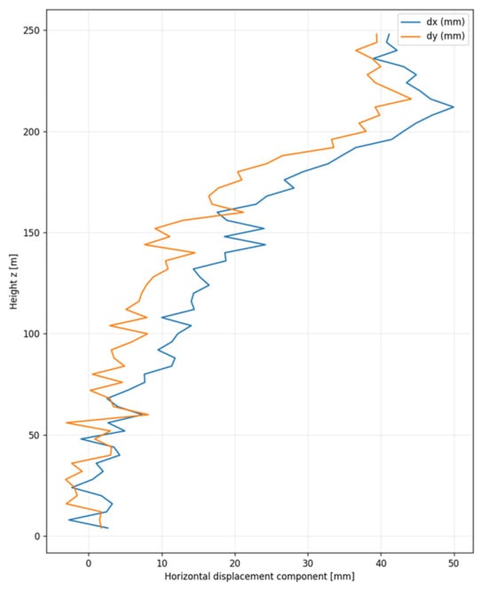
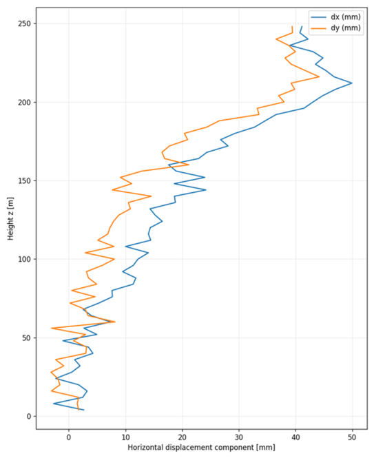
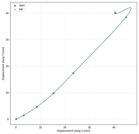
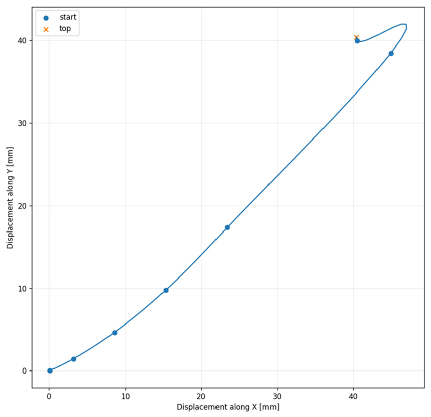
The benchmark uses a hypothetical 248 m, 62-storey geometry with a regular 36 × 24 m plan and five schematic floor points (four corner points and the centre point O). The geometry provides only the elevation grid and the plan-view illustration. A prescribed deformation profile is then imposed according to Equation (8) and propagated to all five floor points as one storey translation. The profile is intentionally selected to cross several decision thresholds, including the highest zone, so that the full escalation logic can be exercised in one numerical stress test. It is not intended to reproduce the response of a particular 248 m building. The five points therefore visualise a common translation and corrective action; they do not represent an independently recovered spatial deformation field. The representative horizontal displacement components are shown in Figure 1, and the deterministic plan-view trajectory is shown in Figure 2.

Figure 1. Horizontal displacement components $d_x$ and $d_y$ for the representative Monte Carlo realisation as a function of height. The T₁–T₃ thresholds are not drawn on the component plot because the decision rule is applied to the resultant magnitude |d|, not separately to $d_x$ or $d_y$.

Figure 2. Deterministic plan-view trajectory defined by the benchmark deformation magnitude and azimuth profile (simulation study).

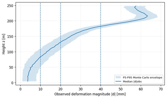
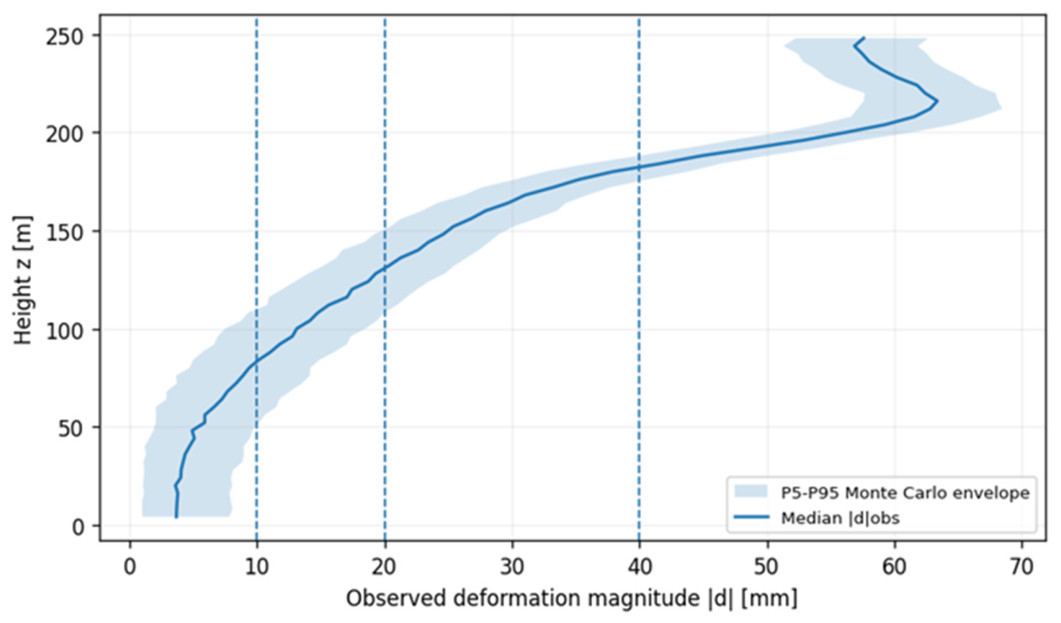
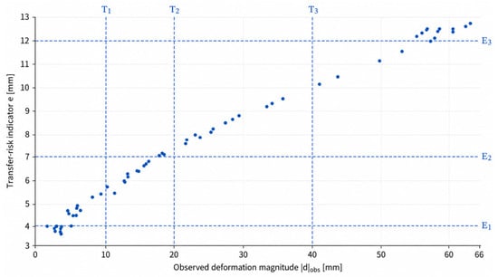
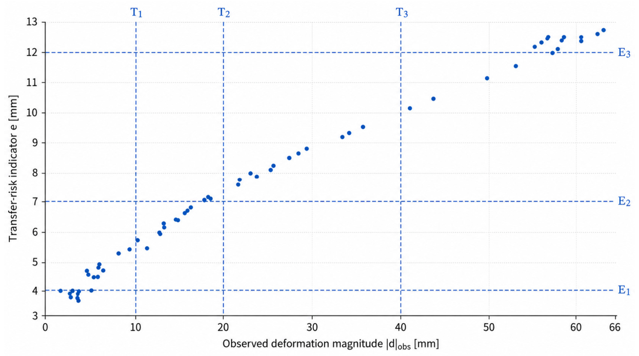
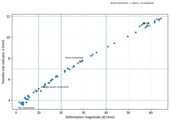
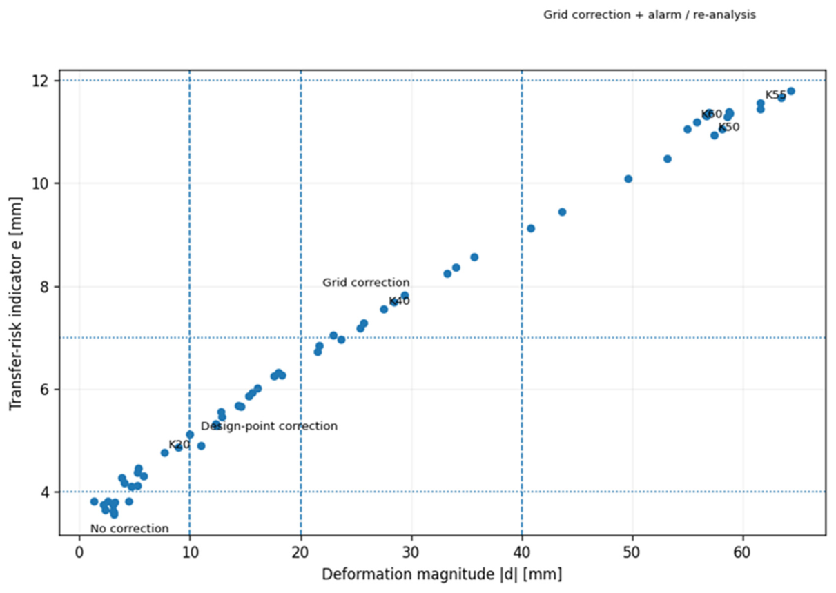
For uncertainty interpretation, Figure 3 presents the Monte Carlo median of the observed deformation magnitude together with the P₅–P₉₅ envelope, rather than a generic “2σ band”. Figure 4 and Figure 5 show the decision plane in terms of deformation magnitude |d| and transfer-risk indicator e.

Figure 3. Median observed deformation magnitude |d| as a function of height with the P₅–P₉₅ Monte Carlo envelope generated from ${\sigma }_{GNSS}$ = 2.5 mm and ${\sigma }_{ref}$ = 2.0 mm; vertical dashed lines show T₁ = 10 mm, T₂ = 20 mm and T₃ = 40 mm.

Figure 4. Decision boundaries in the (${\left|d\right|}_{obs}$, $e_{\mathrm{i}}$) plane. Vertical dashed lines denote the deformation-magnitude thresholds T₁ = 10 mm, T₂ = 20 mm, and T₃ = 40 mm, whereas horizontal dashed lines denote the transfer-risk thresholds E₁ = 4 mm, E₂ = 7 mm, and E₃ = 12 mm. The final decision zone is determined according to the maximum-risk principle.

Figure 5. Operational decision chart showing the maximum-risk response as a function of deformation magnitude |d| and transfer-risk indicator e.

3.2. Results of the Classification of Storeys into Decision Zones

Two types of numerical output are reported. Figure 1, Figure 4, Figure 6 and Figure 7 and Table 2 and Table 3 use one representative uncertainty realisation to illustrate how the rule acts in a single hypothetical measurement campaign, whereas the Monte Carlo envelopes, exceedance probabilities and sensitivity results summarise all 500 realisations. The representative realisation is therefore an illustration of the decision path, not an estimate of how frequently a real building would occupy a given zone. Operational classification uses the resultant deformation magnitude |d| and the transfer-risk indicator e. In the representative realisation, 10 storeys fall in Zone I, 23 in Zone II, 12 in Zone III and 17 in Zone IV under the maximum-risk rule.

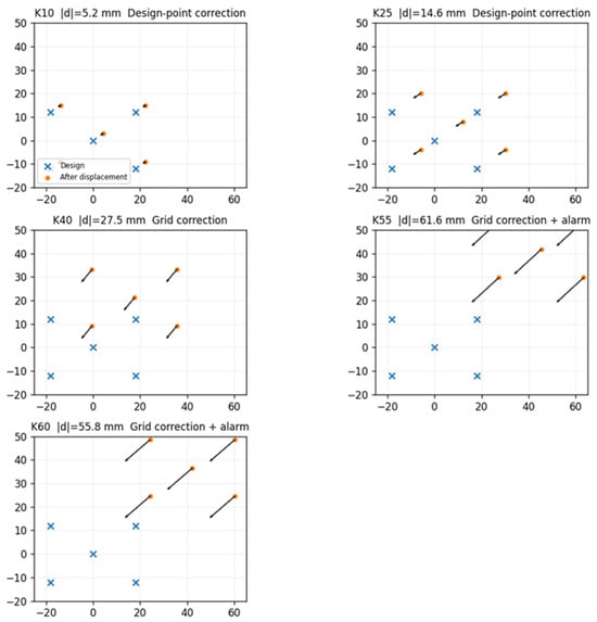
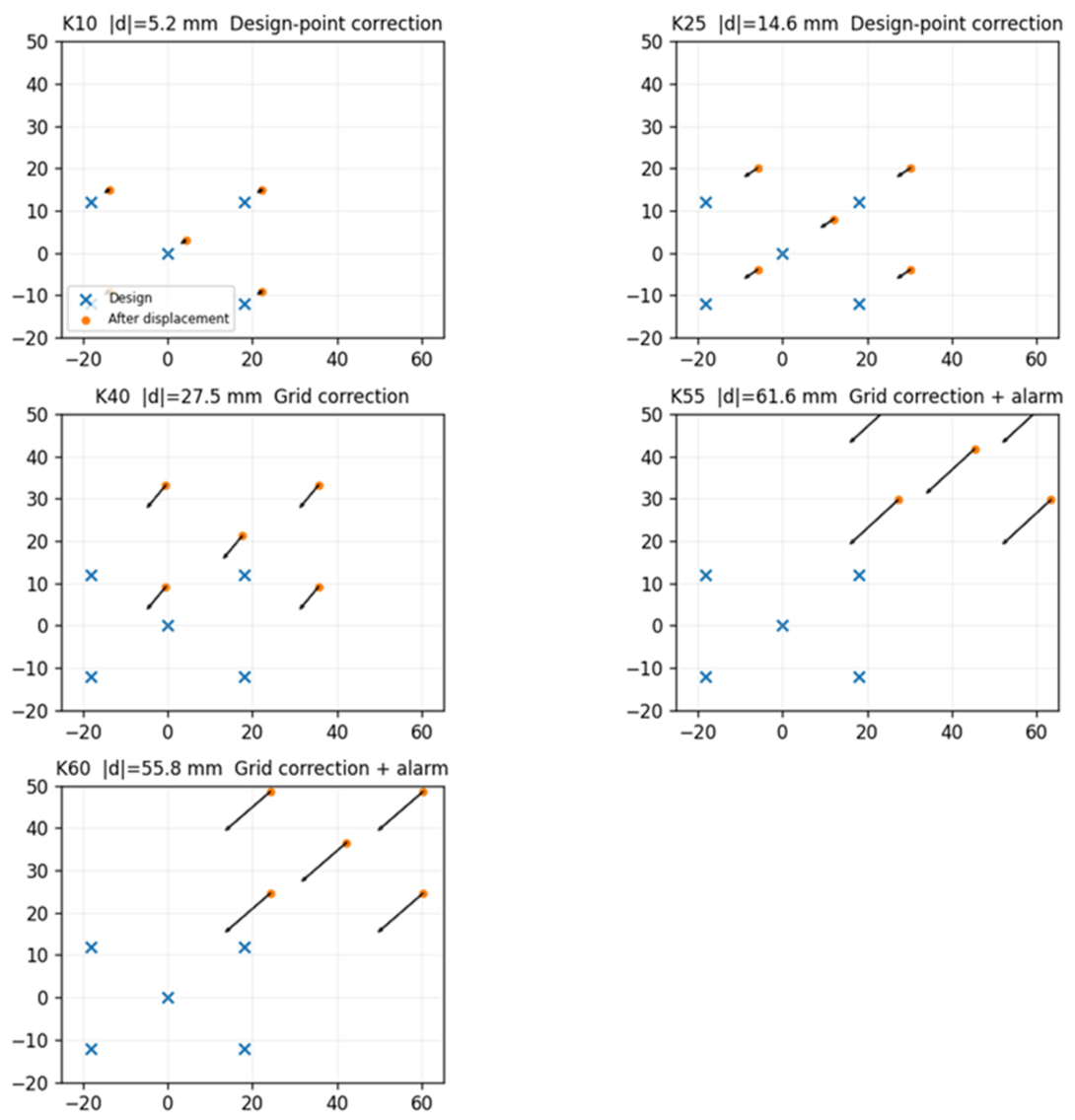
Figure 6. Floor-plan sketches for selected storeys. Design points, translated positions and illustrative correction vectors are shown.

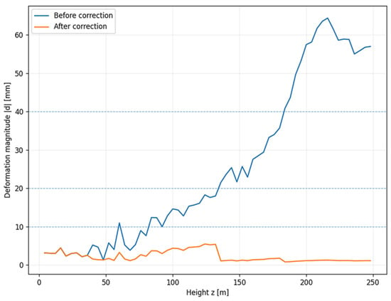
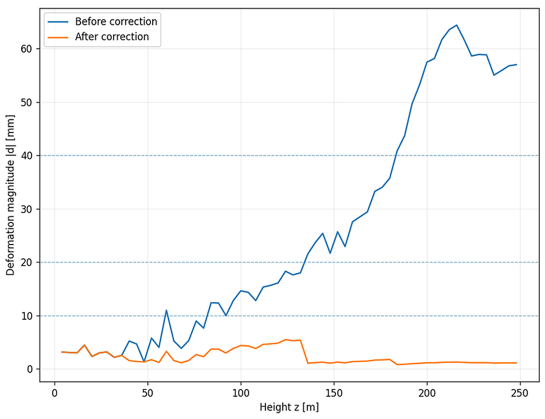
Figure 7. Effectiveness plot for the representative realisation: deformation magnitude before and after the assumed correction as a function of height z [m].

Table 2. Summary of storeys by decision zone for the representative simulation realisation.

Zone	Number of Storeys	Mean |d| [mm]	Maximum |d| [mm]	Mean Transfer-Risk e [mm]	Mean Residual After Correction [mm]
I	10	2.83	4.46	3.71	2.83
II	23	10.96	18.29	5.17	3.29
III	12	27.43	35.70	7.52	1.37
IV	17	56.16	64.35	10.98	1.12

Table 3. Selected representative-storey results from the simulation after application of the maximum-risk decision rule.

Storey	z [m]	${\mathit{d}}_{\mathit{x}}$ [mm]	${\mathit{d}}_{\mathit{y}}$ [mm]	|$\mathit{d}$| [mm]	e [mm]	Decision (Maximum-Risk)	Residual [mm]
1	4.00	2.63	1.74	3.15	3.56	No correction (Zone I)	3.15
10	40.00	4.27	3.01	5.22	4.12	Design-point correction (Zone II)	1.57
20	80.00	7.63	0.52	7.65	4.77	Design-point correction (Zone II)	2.29
30	120.00	14.37	7.27	16.10	6.01	Design-point correction (Zone II)	4.83
40	160.00	17.59	21.19	27.54	7.56	Grid correction (Zone III)	1.38
50	200.00	43.08	37.98	57.43	10.94	Grid correction + alarm/re-analysis (Zone IV)	1.15
55	220.00	45.35	41.72	61.62	11.56	Grid correction + alarm/re-analysis (Zone IV)	1.23
60	240.00	42.21	36.55	55.84	11.19	Grid correction + alarm/re-analysis (Zone IV)	1.12

By definition of the maximum-risk rule, a storey remains in Zone I only when both the observed deformation magnitude satisfies |d| ≤ T₁ and the transfer-risk indicator satisfies e ≤ E₁. In the representative realisation, the mean Zone I value is e = 3.71 mm, below E₁ = 4.00 mm, and no Zone I storey exceeds E₁. Exceeding either first threshold moves the storey to at least Zone II.

3.3. Adjustments to Floor Plans—Sketches and Surveying Interpretation

Figure 6 shows the five-point floor geometry for representative storeys K10, K25, K40, K55 and K60. The five points are shifted by the same storey translation, so the plots illustrate a common translation and the direction of the corresponding corrective action. They do not represent independently estimated rotation, shear or local deformation.

Because the numerical model contains only one resultant translation per storey, Figure 6 should be read as an operational illustration of the translation-based correction rule. Rotation, shear and point-specific deformation require a different, point-resolved observation model.

3.4. Effectiveness of the Correction Procedure Used

The correction stage is also a synthetic scenario component. Zone II removes 70% of the observed storey displacement, Zone III removes 95%, and Zone IV removes 98% and additionally triggers re-analysis. These percentages are assumed intervention efficiencies used to demonstrate propagation of a decision into a residual value; they are not measured performance of GNSS, a total station or a construction process. Figure 7 shows the resulting before/after profiles for the representative realisation. Zone I remains unchanged; the intervention zones have mean residuals of approximately 3.29 mm (Zone II), 1.37 mm (Zone III) and 1.12 mm (Zone IV).

Consequently, the residual values are conditional model outputs. Before field use, the intervention efficiencies must be estimated from independent as-built checks for the actual construction process and surveying configuration.

3.5. Illustrative Decision Scenarios (A–C)

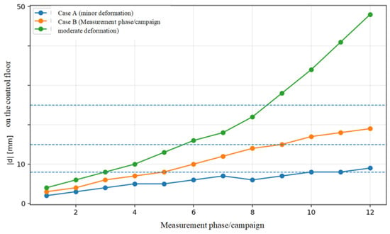
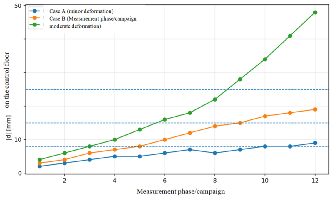
To illustrate the decision logic over successive measurement epochs, three schematic trajectories of deformation magnitude are considered: A—low and stable, B—moderate and increasing, and C—increasing with successive threshold exceedances. These trajectories are illustrative inputs and are not derived from a specific structure. Figure 8 shows how the same quantitative rule would respond to each trajectory. Scenario A remains mainly in Zone I, Scenario B enters Zone II and occasionally Zone III, and Scenario C crosses all thresholds and therefore triggers grid correction together with verification of possible causes. The purpose of this figure is to demonstrate the decision sequence, not to predict a construction history.

Figure 8. Illustrative decision scenarios A–C: threshold exceedances in successive hypothetical measurement campaigns.

3.6. Sensitivity of the Decision Outcomes to the Deformation-Profile Parameters

A local one-at-a-time sensitivity analysis was performed for the three parameters that define the deterministic profile in Equation (8): the trend amplitude a, the trend exponent p and the local-anomaly amplitude A. The baseline values were a = 55 mm, p = 1.6 and A = 20 mm. Each parameter was perturbed by ±20% while the remaining model parameters, thresholds and uncertainty parameters were held fixed. All cases used 500 Monte Carlo realisations with common random numbers. The results in Table 4 therefore quantify the sensitivity of the decision logic to the assumed structural signal rather than to a change in the stochastic forcing.

Table 4. Local sensitivity of the S_I–S_IV decision outcome to the deterministic deformation-profile parameters.

Case	Perturbed Value	Mean Share in Zones III–IV [%]	Height Where P(SIII–IV) ≥ 0.5 [m]	Height Where P(SIV) ≥ 0.5 [m]
Baseline	a = 55 mm; p = 1.60; A = 20 mm	48.4	132	184
a −20%	a = 44 mm	40.9	152	192
a +20%	a = 66 mm	53.9	120	176
p −20%	p = 1.28	55.9	116	180
p +20%	p = 1.92	42.6	148	188
A −20%	A = 16 mm	48.4	132	188
A +20%	A = 24 mm	48.4	132	184

The sensitivity results show that the decision outcome is governed mainly by the global profile parameters a and p. Increasing a by 20% raises the mean share of storeys in Zones III–IV from 48.4% to 53.9% and moves the 50% probability onset of Zones III–IV from 132 m to 120 m; decreasing a reduces the share to 40.9% and shifts the onset to 152 m. Decreasing p from 1.60 to 1.28 increases the power-law term over most of the height, raising the Zones III–IV share to 55.9% and moving its 50% onset to 116 m, whereas increasing p to 1.92 reduces the share to 42.6% and shifts the onset to 148 m. Changing A by ±20% leaves the overall Zones III–IV share essentially unchanged at 48.4% because A controls only a localised upper-storey anomaly; its main effect is a small shift in the onset of Zone IV. These results quantify the sensitivity of the classifier to the prescribed benchmark signal and reinforce the need for project-specific calibration before field use.

4. Discussion

The main contribution of the study is the operational decision layer rather than a complete GNSS network solution or a structural deformation model. GNSS enters at the processed coordinate-solution level through independent horizontal coordinate noise and a campaign-common reference-frame bias. The Monte Carlo procedure then propagates these uncertainties through the decision rule. It does not simulate raw carrier-phase observations, satellite geometry, ambiguity resolution, a point-by-point least-squares adjustment, structural loads or material response. The results should therefore be interpreted as a controlled test of the decision logic that could later be coupled to GNSS, total-station or hybrid observations.

The synthetic nature of Equation (8) is an important limitation. The power-law plus localised bell-shaped profile is chosen because it provides two clearly controlled deformation patterns and forces the classifier to cross multiple thresholds; it is not evidence that a real 248 m building will deform in this form or to this magnitude. Likewise, the thresholds, transfer-risk coefficients and 70/95/98% intervention efficiencies are scenario parameters. A field application must replace these inputs with measured deformation histories or a structurally validated model, project tolerances and empirically determined correction performance. The present results therefore demonstrate algorithmic behaviour and sensitivity, not structural realism.

The numerical uncertainty model is intentionally compact. ${\sigma }_{GNSS}$ = 2.5 mm and ${\sigma }_{ref}$ = 2.0 mm are favourable scenario values, not universal accuracies. The common ${\sigma }_{ref}$ term creates correlation between storeys within one campaign, but many real construction-site effects remain outside the model, including façade/reinforcement multipath, crane masking, changing satellite geometry, atmospheric correlation, antenna instability and temporal correlation. These limitations are important when transferring the framework to field data.

For field application, the treatment of structural movement is equally important. Wind- and temperature-induced displacements may be reversible, and redefining a construction grid to follow an instantaneous elastic deflection could itself introduce a systematic setting-out error once the structure returns towards its mean position. The operational workflow should therefore include a persistence test based on repeated observations, time averaging and environmental or SHM information before a geometric correction is authorised. Persistent settlement or quasi-static drift should be distinguished from transient elastic response and from local technological effects such as differential shortening. This motivates a two-layer concept: a geodetic reference layer and a separate construction-compensation layer.

A practical field implementation should be hybrid rather than GNSS-only. Periodic static or rapid-static GNSS ties can maintain the relationship to an external datum, while total stations and optical/laser plummets can provide relative floor geometry and vertical transfer, especially where satellite visibility is poor. Inclinometers and other SHM sensors may provide supporting evidence about transient structural response. The decision layer itself does not require GNSS as long as the displacement estimate, uncertainty information and datum relationship are controlled.

The next research stage is an observation-level validation. A field study should document receiver/antenna configuration, observation duration, reference-station geometry, processing strategy, quality indicators and independent checks. A subsequent numerical model should simulate point-specific observations, full network adjustment, rotation/shear/local deformation, realistic spatial-temporal covariance and method-to-method comparison. This would allow the same S_I–S_IV decision logic to be tested using GNSS-only, conventional-geodetic and hybrid control solutions.

5. Conclusions

The conclusions below refer only to the synthetic benchmark and the stated uncertainty and decision assumptions:

• Under the synthetic benchmark, the four-zone maximum-risk operator provides an internally consistent escalation rule from monitoring to design-point correction, grid correction and alarm/re-analysis. In the representative uncertainty realisation, 10, 23, 12 and 17 storeys fall in Zones I–IV, respectively.
• The residual values are conditional on ${\sigma }_{GNSS}$ = 2.5 mm, ${\sigma }_{ref}$ = 2.0 mm, the transfer-risk coefficients and the assumed 70/95/98% intervention efficiencies. Mean residuals in the representative realisation are about 3.29 mm in Zone II, 1.37 mm in Zone III, and 1.12 mm in Zone IV; these values are benchmark outputs and not demonstrated field accuracy.
• The Monte Carlo analysis represents repeated measurement-uncertainty realisations for one fixed prescribed deformation profile. It quantifies the stability of threshold crossing and zone assignment; it does not estimate structural-event probabilities and it is not a full GNSS control-network adjustment.
• Equation (8) is a synthetic stress-test signal combining a global height-dependent component with a localised bell-shaped anomaly. Its parameters are chosen to exercise the decision zones, not to predict deformation of a particular building; field application requires measured or structurally validated deformation inputs.
• The sensitivity analysis shows that the global profile parameters materially affect the height at which intervention becomes likely: for the tested ±20% changes, the 50% onset of Zones III–IV shifts from 120 to 152 m for parameter a and from 116 to 148 m for parameter p. This confirms that decision thresholds cannot be interpreted independently of the deformation model used as input.
• Field validation is therefore essential. Further work should include measured deformation histories, point-by-point network adjustment, full covariance and reliability analysis, comparison of GNSS and conventional surveying solutions, tests of control-point density and geometry, and empirical calibration of the thresholds, transfer-risk coefficients, and correction efficiencies.

References

- Im, S.B.; Hurlebaus, S.; Kang, Y.J. Summary Review of GPS Technology for Structural Health Monitoring. J. Struct. Eng. 2013, 139, 1653–1664. [Google Scholar] [CrossRef] [Scilit]
- Shan, J.; Zhang, H.; Shi, W.; Lu, X. Health monitoring and field-testing of high-rise buildings: A review. Struct. Concr. 2020, 21, 1272–1285. [Google Scholar] [CrossRef] [Scilit]
- Su, J.; Xia, Y.; Weng, S. Review on field monitoring of high-rise structures. Struct. Control Health Monit. 2020, 27, e2629. [Google Scholar] [CrossRef] [Scilit]
- Yang, Y.; Xu, W.; Gao, Z.; Yu, Z.; Zhang, Y. Research Progress of SHM System for Super High-Rise Buildings Based on Wireless Sensor Network and Cloud Platform. Remote Sens. 2023, 15, 1473. [Google Scholar] [CrossRef] [Scilit]
- Yi, T.-H.; Li, H.-N.; Gu, M. Recent Research and Applications of GPS-Based Monitoring Technology for High-Rise Structures. Struct. Control Health Monit. 2013, 20, 649–670. [Google Scholar] [CrossRef] [Scilit]
- Zhang, X.; Zhang, Y.; Li, B.; Qiu, G. GNSS-Based Verticality Monitoring of Super-Tall Buildings. Appl. Sci. 2018, 8, 991. [Google Scholar] [CrossRef] [Scilit]
- Quesada-Olmo, N.; Jimenez-Martinez, M.J.; Farjas-Abadia, M. Real-time high-rise building monitoring system using global navigation satellite system technology. Measurement 2018, 123, 115–124. [Google Scholar] [CrossRef] [Scilit]
- Lovse, J.W.; Teskey, W.F.; Lachapelle, G.; Cannon, M.E. Dynamic Deformation Monitoring of Tall Structure Using GPS Technology. J. Surv. Eng. 1995, 121, 35–40. [Google Scholar] [CrossRef] [Scilit]
- Tamura, Y.; Matsui, M.; Pagnini, L.-C.; Ishibashi, R.; Yoshida, A. Measurement of wind-induced response of buildings using RTK-GPS. J. Wind Eng. Ind. Aerodyn. 2002, 90, 1783–1793. [Google Scholar] [CrossRef] [Scilit]
- Park, H.S.; Sohn, H.G.; Kim, I.S.; Park, J.H. Application of GPS to monitoring of wind-induced responses of high-rise buildings. Struct. Des. Tall Build. 2008, 17, 117–132. [Google Scholar] [CrossRef] [Scilit]
- Yi, T.-H.; Li, H.-N.; Gu, M. Experimental assessment of high-rate GPS receivers for deformation monitoring of bridge. Measurement 2013, 46, 420–432. [Google Scholar] [CrossRef] [Scilit]
- He, Y.; Han, X.; Li, Q.; Zhu, H.; He, Y. Monitoring of wind effects on 600 m high Ping-An Finance Center during Typhoon Haima. Eng. Struct. 2018, 167, 308–326. [Google Scholar] [CrossRef] [Scilit]
- Su, J.Z.; Xia, Y.; Zhu, L.D.; Zhu, H.P.; Ni, Y.Q. Typhoon- and temperature-induced quasi-static responses of a supertall structure. Eng. Struct. 2017, 143, 91–100. [Google Scholar] [CrossRef] [Scilit]
- Li, Q.S.; Zhi, L.H.; Yi, J.; To, A.; Xie, J. Monitoring of typhoon effects on a super-tall building in Hong Kong: Monitoring of Typhoon Effects. Struct. Control Health Monit. 2014, 21, 926–949. [Google Scholar] [CrossRef] [Scilit]
- Yi, J.; Li, Q.S. Wind tunnel and full-scale study of wind effects on a super-tall building. J. Fluids Struct. 2015, 58, 236–253. [Google Scholar] [CrossRef] [Scilit]
- Choi, S.; Kim, Y.; Kim, J.; Park, H. Field Monitoring of Column Shortenings in a High-Rise Building during Construction. Sensors 2013, 13, 14321–14338. [Google Scholar] [CrossRef] [Scilit] [PubMed]
- Samarakkody, D.I.; Thambiratnam, D.P.; Chan, T.H.T.; Moragaspitiya, P.H.N. Differential axial shortening and its effects in high rise buildings with composite concrete filled tube columns. Constr. Build. Mater. 2017, 143, 659–672. [Google Scholar] [CrossRef] [Scilit]
- Elansary, A.; Metwally, M.I.; El-Attar, A. Assessment of mitigation alternatives for differential shortening in high-rise reinforced concrete buildings. J. Eng. Appl. Sci. 2023, 70, 152. [Google Scholar] [CrossRef] [Scilit]
- Moragaspitiya, P.; Thambiratnam, D.; Perera, N.; Chan, T. A numerical method to quantify differential axial shortening in concrete buildings. Eng. Struct. 2010, 32, 2310–2317. [Google Scholar] [CrossRef] [Scilit]
- Park, H.S. Optimal compensation of differential column shortening in high-rise buildings. Struct. Des. Tall Build. 2003, 12, 49–66. [Google Scholar] [CrossRef] [Scilit]
- Woo Park, S.; Woon Choi, S.; Seon Park, H. Moving average correction method for compensation of differential column shortenings in high-rise buildings. Struct. Des. Tall Build. 2013, 22, 718–728. [Google Scholar] [CrossRef] [Scilit]
- Yu, L.; Xiong, C.; Chen, W.; Gao, Y.; Ye, Z.; Shi, Q. A combined algorithm for denoising GNSS-RTK positioning solutions with application to displacement monitoring of a super-high-rise building. Meas. Sci. Technol. 2021, 32, 115121. [Google Scholar] [CrossRef] [Scilit]
- Yigit, C.O.; Bezcioglu, M.; Ilci, V.; Ozulu, I.M.; Alkan, R.M.; Dindar, A.A.; Karadeniz, B. Assessment of Real-Time PPP with Trimble RTX correction service for real-time dynamic displacement monitoring based on high-rate GNSS observations. Measurement 2022, 201, 111704. [Google Scholar] [CrossRef] [Scilit]
- Xiong, C.; Shang, Z.; Wang, M. Improved Hybrid Denoising Method for Dynamic Monitoring of a Super-High-Rise Building Based on a GNSS-RTK Technique. J. Struct. Eng. 2024, 150, 04024116. [Google Scholar] [CrossRef] [Scilit]
- Xiao, X.; Han, H.; Wang, J.; Li, D.; Chen, C.; Wang, L. Dynamic Deformation Analysis of Super High-Rise Buildings Based on GNSS and Accelerometer Fusion. Sensors 2025, 25, 2659. [Google Scholar] [CrossRef] [Scilit] [PubMed]
- ISO 4463-1:1989; Measurement Methods for Building—Setting-Out and Measurement—Part 1: Planning and Organization, Measuring Procedures, Acceptance Criteria. International Organization for Standardization: Geneva, Switzerland, 1989.
- EN 13670:2009; Execution of Concrete Structures. European Committee for Standardization: Brussels, Belgium, 2009.
Disclaimer/Publisher’s Note: The statements, opinions and data contained in all publications are solely those of the individual author(s) and contributor(s) and not of MDPI and/or the editor(s). MDPI and/or the editor(s) disclaim responsibility for any injury to people or property resulting from any ideas, methods, instructions or products referred to in the content. |
© 2026 by the authors. Licensee MDPI, Basel, Switzerland. This article is an open access article distributed under the terms and conditions of the Creative Commons Attribution (CC BY) license.