


Abstract
We propose a novel hybrid architecture that integrates a continuous-time Liquid Neural Network with an optimized Long Short-Term Memory network for seismic vulnerability state assessment of ancient halls. The proposed system processes multi-source structural monitoring data, including acceleration, strain, displacement, temperature, and humidity signals. A central challenge in this domain is the long-term state drift that occurs when continuous-time models are exposed to prolonged seismic events or sequences of aftershocks. To address this issue, we introduce a learnable event-triggered discrete reset mechanism that monitors a prediction error signal and an auxiliary drift accumulation variable. When a trigger condition is met, the Liquid Neural Network hidden state is reinitialized to a learned baseline state, thereby preventing divergence from physically plausible structural dynamics. This reset mechanism is inspired by hybrid small-gain and impulsive control frameworks and provides rigorous stability guarantees. The continuous-time dynamics are modeled as a neural ordinary differential equation with a sinusoidal activation function, solved via a fixed-step Runge–Kutta integrator. The discrete-time pathway employs a two-layer LSTM with Bayesian-optimized hyperparameters. A learned attention mechanism fuses the hidden states from both pathways, and the combined representation is passed through a feedforward network to produce a four-class seismic vulnerability index. The entire system is trained end-to-end with an adaptive loss function that balances reconstruction accuracy, drift penalization, and classification performance. We first pre-train the model on synthetic data generated from a calibrated finite element model of a representative ancient hall in Rucheng, Hunan. Transfer learning then fine-tunes the model on real monitoring data. Our approach replaces conventional fragility-curve-based estimates with a data-driven, adaptive vulnerability assessment that is site-specific and robust to non-stationary excitation. The hybrid switched-system framework therefore offers a principled solution to the state drift problem while maintaining the expressive power of continuous-time neural dynamics.
1. Introduction
Structural health monitoring (SHM) of heritage buildings, particularly ancient timber halls, presents unique challenges due to their complex structural systems, material degradation over centuries, and the need for non-invasive sensing [1]. Traditional approaches to seismic vulnerability state assessment have relied heavily on finite element modeling and modal analysis, often supplemented by statistical pattern recognition techniques applied to sensor data [2,3]. While these methods provide valuable baseline assessments, they struggle to capture the nonlinear, time-varying dynamics that characterize structural responses during seismic events, especially when multiple sensor modalities (e.g., acceleration, strain, displacement, temperature, and humidity) must be fused into a unified vulnerability metric [4].
The advent of deep learning has introduced powerful tools for processing time-series sensor data in SHM applications [5,6]. Among recurrent architectures, the Long Short-Term Memory (LSTM) network has become a cornerstone for capturing long-term temporal dependencies in vibration signals, effectively addressing the vanishing gradient problem inherent in vanilla RNNs [7,8]. Subsequent research has focused on optimizing LSTM hyperparameters and architectures using evolutionary algorithms to enhance prediction accuracy for structural displacement and acceleration [9]. However, these discrete-time models operate on fixed sampling intervals and may not adequately represent the continuous physical processes governing structural dynamics.
More recently, machine learning techniques have been extended to address the cumulative damage of structures under seismic sequences. Petros C. Lazaridis et al. [10] employed SHAP, LIME, and Partial Dependence Plots to identify the most critical predictors for cumulative damage in an eight-story RC frame subjected to mainshock–aftershock sequences, revealing that the pre-existing damage from the first shock and the intensity measures of the subsequent shock—particularly IFVF and SIH—are the most influential features. Concurrently, Md. Hasan Imam et al. [11] proposed a deep learning-based framework for rapid post-earthquake damage assessment of RC frames under mainshock–aftershock sequences, incorporating pre-earthquake damage, structural parameters, and ground motion characteristics as inputs to predict story-level and global damage indices. These studies underscore the growing recognition that seismic vulnerability assessment must account for the accumulation of damage across multiple events, yet they primarily focus on reinforced concrete frames and discrete-time modeling schemes, leaving the challenge of continuous-time state drift in heritage timber structures under prolonged seismic sequences largely unaddressed.
Parallel to these developments, the field of neural differential equations has emerged, leading to the formulation of Neural Ordinary Differential Equations (Neural ODEs) that model continuous-depth networks [12,13]. Building upon this foundation, Liquid Neural Networks (LNNs) were proposed to utilize time-continuous hidden states governed by differential equations, offering superior adaptability to non-stationary inputs and causal reasoning in time-series data [14]. These liquid time-constant networks have demonstrated promise in robotics and control tasks requiring real-time adaptation, yet their application to multi-source structural monitoring remains largely unexplored. A critical limitation of continuous-time models in this context is the phenomenon of long-term state drift, where the hidden state gradually diverges from physically plausible dynamics when the model is exposed to prolonged seismic events or sequences of aftershocks.
To manage complex dynamic behaviors, hybrid systems theory provides a rigorous mathematical framework combining continuous flows and discrete jumps, often analyzed using Lyapunov stability methods [15,16]. Within this domain, impulsive control strategies and event-triggered control mechanisms have been extensively studied to stabilize systems while minimizing communication or computational load [17]. The concept of resetting neural states to prevent drift draws inspiration from reset control systems in classical control theory, such as the Clegg integrator, which resets state variables upon crossing zero to reduce overshoot [18]. In machine learning, recent works have explored hard attention mechanisms and gating strategies that function similarly to discrete resets, though a formal integration with small-gain theorems for stability guarantees in hybrid neural architectures is an emerging direction [19].
In this paper, we propose a novel hybrid state-space architecture that integrates continuous-time LNN dynamics with an optimized LSTM network, enhanced by a learnable event-triggered discrete reset mechanism to prevent long-term state drift in multi-source structural monitoring data. The LNN layer captures fast, nonlinear transient responses from sensor streams (e.g., acceleration, strain, displacement) using neural ODEs, while the LSTM layer models slower temporal dependencies and multi-scale features. To address state drift under prolonged seismic events, we introduce a dynamic event-triggered reset controller inspired by hybrid small-gain and impulsive control frameworks, where a learnable trigger condition decides when to reset or reinitialize the hidden states based on prediction error and monitoring anomalies. This event-triggered hybrid dynamics is formulated as a switched system with auxiliary dynamic variables, enabling rigorous stability analysis and finite-time convergence guarantees. The combined model outputs a seismic vulnerability index for ancient halls, trained end-to-end with an adaptive loss function that balances reconstruction accuracy, drift penalty, and classification performance.
The key contributions of this work are threefold. First, we propose a principled fusion of continuous-time liquid dynamics with discrete event-driven resets, which uniquely addresses the state drift problem that has hindered the application of continuous-time neural models to long-duration SHM tasks. Second, we provide rigorous stability guarantees for the hybrid switched system through a small-gain analysis framework, ensuring that the model’s hidden states remain bounded and converge to physically plausible trajectories even under non-stationary excitation. Third, we demonstrate the practical effectiveness of our approach through a comprehensive experimental study on both synthetic data generated from a calibrated finite element model of a representative ancient hall in Rucheng, Hunan, and real monitoring data collected from the same structure.
It is important to clarify the terminology used in this study. The proposed model outputs a four-class damage state label for each 30-second monitoring window, which we refer to as the “seismic vulnerability index.” This terminology follows the usage in recent structural health monitoring literature, where “vulnerability assessment” denotes the real-time or near-real-time evaluation of a structure’s current damage state based on direct sensor measurements. This differs from, yet complements, the classical probabilistic seismic fragility analysis, which expresses the conditional probability of exceeding a given damage state as a function of ground motion intensity (e.g., ). In the present framework, fragility curves are not directly constructed; rather, the finite element model serves as a physics-based data generator that bridges the gap between intensity-based probabilistic assessments and sensor-driven classification models.
The remainder of this paper is organized as follows. Section 2 reviews related work in structural health monitoring, liquid neural networks, and hybrid control systems. Section 3 provides the necessary preliminaries on LNNs, LSTM networks, and event-triggered control theory. Section 4 presents the proposed hybrid liquid-state LSTM architecture with learnable event-triggered resets in detail. Section 5 describes the experimental setup, including data collection, preprocessing, and training procedures. Section 6 reports and analyzes the experimental results. Section 7 discusses the implications of our findings and outlines directions for future research. Section 8 concludes the paper with a summary of our contributions.
2. Related Work
2.1. Deep Learning for Structural Health Monitoring
The application of deep learning to structural health monitoring has grown substantially over the past decade, driven by the increasing availability of multi-sensor data and the need for automated damage detection [20,21]. The foundational concepts of recurrent neural networks (RNNs) [22] and convolutional neural networks (CNNs) [23] have established the bedrock of modern deep learning feature extraction. Among recurrent architectures, the Long Short-Term Memory (LSTM) network, originally introduced by Hochreiter and Schmidhuber [24], has been widely adopted for modeling temporal dependencies in vibration signals, as it effectively mitigates the vanishing gradient problem that plagues standard RNNs [25,26]. For example, researchers have employed LSTM networks to predict nonlinear seismic responses of building structures, demonstrating superior performance compared to traditional autoregressive models [27]. More recently, hybrid architectures combining convolutional neural networks with LSTM layers have been proposed for extracting both spatial and temporal features from multi-channel sensor data, achieving improved accuracy in damage classification tasks [28]. However, these discrete-time models operate on fixed sampling intervals and may not adequately capture the continuous physical processes governing structural dynamics, particularly during rapid transient events such as earthquake ground motions.
Parallel to the development of deep learning for SHM, recent studies have increasingly employed data-driven methods to assess the seismic performance of structural components. For instance, machine learning frameworks based on Random Forest and XGBoost have been applied to predict the deformation capacity of steel-reinforced concrete columns using extensive test databases, achieving substantial improvements over conventional empirical formulas [29]. Similarly, Transformer-based architectures have been introduced to evaluate the plastic hinge length of reinforced concrete columns, with SHAP analysis providing interpretability of the underlying structural parameters [30]. Experimental investigations on steel–concrete composite members under seismic loading have further validated the mechanical basis for these data-driven approaches [31]. These developments underscore the growing synergy between machine learning and structural engineering, motivating the integration of advanced neural architectures—such as the hybrid LSTM-LNN framework proposed in this study—for more robust and interpretable seismic vulnerability assessment.
2.2. Liquid Neural Networks and Neural ODEs
The seminal framework of Neural Ordinary Differential Equations (Neural ODEs), pioneered by Kim et al. [32], introduced a paradigm shift by modeling continuous-depth networks through differential equations, enabling adaptive computation and memory-efficient gradient computation [33]. Building on this foundation, Liquid Neural Networks (LNNs) were proposed to utilize time-continuous hidden states governed by neural ODEs, offering superior adaptability to non-stationary inputs and causal reasoning in time-series data [34,35]. These liquid time-constant networks have demonstrated remarkable performance in robotics and control tasks requiring real-time adaptation, such as autonomous driving and drone navigation, where they can adjust their dynamics in response to changing environmental conditions. In the context of fault diagnosis, a liquid-impulse neural network model was recently proposed for rotating machinery, integrating a liquid layer with an impulse mechanism that resets the membrane potential upon detecting anomalies [36]. This work shares conceptual similarities with our approach, as both employ a reset mechanism to prevent state drift. However, the reset in that model is triggered by a fixed threshold on the membrane potential, whereas our event-triggered mechanism is learnable and incorporates an auxiliary dynamic variable that accumulates drift over time, providing greater flexibility and adaptability to site-specific structural characteristics.
2.3. Event-Triggered Control and Hybrid Systems
Event-triggered control has been extensively studied in control theory as a means to reduce communication and computational load while maintaining system stability [37,38]. The core idea is to update the control input only when a predefined condition is violated, rather than at every sampling instant. A seminal work in this area interpreted event-triggered controlled systems as the interconnection of hybrid dynamical systems and analyzed the overall system using a hybrid small-gain theorem, providing a rigorous framework for stability analysis [39]. This perspective is particularly relevant to our work, as we model the proposed architecture as a hybrid switched system with continuous-time LNN dynamics and discrete event-triggered resets. Furthermore, finite-time stability of dynamical systems under event-triggered hybrid control has been investigated, combining impulsive control and sampling control mechanisms to achieve convergence within a bounded time interval [40]. These theoretical foundations inform the stability guarantees we provide for our hybrid architecture. More recently, distributed hybrid dynamic event-triggered consensus control has been proposed for nonlinear multi-agent systems, where the trigger condition involves additional dynamic variables governed by differential equations [41]. This dynamic event-triggered approach is closely related to our learnable trigger mechanism, which incorporates an auxiliary drift accumulation variable to improve robustness against prolonged excitation.
2.4. Comparison with Existing Methods
While existing works have explored LSTM networks for seismic response prediction [42], liquid neural networks for fault diagnosis [43,44], and event-triggered control for hybrid systems [45], none have integrated these three components into a unified framework for seismic vulnerability state assessment. The key novelty of our proposed approach lies in the principled fusion of continuous-time liquid dynamics with discrete event-driven resets, where the trigger condition is learnable and incorporates an auxiliary dynamic variable that accumulates drift over time. This design uniquely addresses the state drift problem that has hindered the application of continuous-time neural models to long-duration SHM tasks, while the hybrid small-gain analysis framework provides rigorous stability guarantees that are absent in purely data-driven approaches. Furthermore, our architecture is specifically tailored to multi-source structural monitoring data from ancient halls, incorporating a learned attention mechanism for fusing continuous-time and discrete-time representations and an adaptive loss function that balances reconstruction accuracy, drift penalization, and classification performance.
3. Preliminaries: Liquid Neural Networks, LSTM, and Event-Triggered Control
This section establishes the foundational concepts necessary to understand the proposed hybrid architecture. We begin by reviewing discrete-time recurrent neural networks and their limitations in modeling continuous physical processes, then introduce neural ordinary differential equations as a continuous-time alternative, and finally discuss hybrid dynamical systems and event-triggered control theory that inform our learnable reset mechanism.
3.1. Foundations of Discrete Recurrent Architectures and Temporal Dependency Modeling
Recurrent neural networks (RNNs) and their variants form the backbone of sequence modeling in deep learning. A discrete-time RNN approximates a dynamical system by updating its hidden state at each time step according to the recurrence relation:
where is the hidden state at time step , is the input vector, and is a parameterized nonlinear function typically implemented as a neural network layer. The Long Short-Term Memory (LSTM) network addresses the vanishing gradient problem inherent in vanilla RNNs by introducing a gating mechanism that controls information flow through input, forget, and output gates. This architecture enables the network to maintain long-term dependencies over hundreds of time steps, making it particularly suitable for modeling structural vibration signals that exhibit both rapid transient responses and slow modal decay.
Despite their success, discrete-time recurrent models operate on fixed sampling intervals and implicitly assume that the underlying dynamics can be adequately captured at the chosen sampling rate. For structural health monitoring applications involving seismic events, the ground motion excitation contains frequency components that may exceed the Nyquist frequency of the sensor sampling rate, leading to aliasing artifacts. Moreover, the discrete-time formulation does not naturally accommodate irregularly sampled data or variable-rate sensor streams, which are common in multi-source monitoring systems where different sensors may operate at different sampling frequencies.
3.2. Neural Ordinary Differential Equations and Continuous-Time Dynamics
To overcome the limitations of discrete-time models, Neural Ordinary Differential Equations (Neural ODEs) parameterize the derivative of the hidden state with respect to time using a neural network. The continuous-time dynamics are governed by:
where is a neural network with parameter , and evolves continuously from an initial condition . The hidden state at any desired time point can be obtained by solving the initial value problem using numerical ODE solvers such as Runge–Kutta methods. This formulation allows the model to handle irregularly sampled data naturally, as the ODE solver can evaluate the dynamics at arbitrary time points.
Liquid Neural Networks (LNNs) extend this framework by incorporating time-varying parameters and nonlinearities that enable the network to adapt its dynamics in response to changing input conditions. A key property of LNNs is their ability to maintain stable dynamics through Lipschitz continuity constraints on the derivative function. Specifically, the function in Equation (2) must satisfy:
For some Lipschitz constant , ensuring that small perturbations in the hidden state do not lead to unbounded divergence over time. This Lipschitz condition is crucial for the stability of continuous-time neural models, as it guarantees that the solution trajectory remains bounded under bounded inputs. However, even with Lipschitz continuity, prolonged exposure to non-stationary inputs—such as sequences of aftershocks following a major seismic event—can cause the hidden state to drift away from physically plausible trajectories, motivating the need for a reset mechanism.
3.3. Hybrid Dynamical Systems and Event-Triggered Control Theory
Hybrid dynamical systems combine continuous-time evolution with discrete instantaneous changes, providing a natural framework for modeling systems that exhibit both smooth dynamics and abrupt state transitions. A general representation of such systems is given by the impulsive differential equation:
where is the state vector, governs the continuous flow between events, and defines the discrete jump at trigger times . The notation and denote the state immediately before and after the jump, respectively. This formulation is widely used in control theory to model systems with resets, impulses, or switching behaviors.
Event-triggered control determines the trigger times based on the system state rather than a fixed time schedule, reducing communication and computational overhead while maintaining stability. A common approach is to define a triggering condition based on a Lyapunov function , where the control input is updated only when the derivative condition:
The derivative condition is violated for some . This condition ensures that the Lyapunov function decays exponentially during inter-event intervals, guaranteeing asymptotic stability. The hybrid small-gain theorem provides a rigorous framework for analyzing the stability of interconnected hybrid systems, where the continuous and discrete dynamics are treated as subsystems with input-output gains. This theorem is particularly relevant to our proposed architecture, as the LNN dynamics and the event-triggered reset mechanism can be viewed as two interacting subsystems whose combined behavior must be stable.
4. Hybrid Liquid-State LSTM with Learnable Event-Triggered Resets
We now present the proposed hybrid architecture in detail. The system integrates a continuous-time Liquid Neural Network with a discrete-time optimized LSTM, governed by a learnable event-triggered reset mechanism that prevents long-term state drift. The overall architecture is designed to process multi-source structural monitoring data streams and produce a seismic vulnerability index for ancient halls. We first describe the system-level integration, and then detail the internal components including the LNN dynamics, the LSTM pathway, the event-triggered reset mechanism, and the attention-based fusion layer.
Before delving into the mathematical formulations of each component, it is important to clarify the distinct physical roles of the five sensor modalities within the proposed multi-source framework. Acceleration, strain, and displacement signals directly encode the mechanical response of the structure to seismic or ambient excitations, and are therefore treated as primary dynamic inputs to both the continuous-time and discrete-time pathways. In contrast, temperature and humidity are not direct measures of structural vibration, but rather environmental modulators that alter the instantaneous material properties of ancient timber structures. Specifically, variations in ambient temperature and moisture content influence the elastic modulus, friction coefficients at mortise–tenon joints, and dowel-bearing capacity of aged wood, thereby affecting the structural stiffness and energy dissipation characteristics prior to or during seismic excitation. Within our data-driven vulnerability state assessment, these environmental signals serve as contextual covariates that help the model disambiguate whether observed changes in mechanical sensor readings arise from seismic-induced damage or from reversible hygrothermal expansions and contractions. By feeding temperature and humidity as time-varying external inputs to the continuous-time LNN dynamics alongside the mechanical channels, the model learns a conditional mapping where the same acceleration or strain pattern may be interpreted differently under distinct environmental contexts. This formulation enhances robustness against false alarms during diurnal or seasonal ambient variations and is consistent with the hybrid system paradigm, where slow environmental dynamics interact with fast structural transients through the same neural ODE framework.
It is important to clarify that temperature and humidity are not generated as direct mechanical outputs of the nonlinear seismic FE analysis. Rather, these environmental variables are prescribed as time-varying boundary conditions that modulate the instantaneous material properties of the timber structure. Specifically, the longitudinal elastic modulus , radial modulus , and tangential modulus of the aged Chinese fir are degraded by a linear reduction factor of 2.1% per 1% increase in moisture content above the 12% reference level, based on the experimentally derived hygrothermal relationships from the material characterization study. The ambient temperature time series are imposed as sinusoidal diurnal cycles (amplitude ±8 °C about a daily mean) superimposed with seasonal trends, while relative humidity is modeled as a first-order autoregressive process correlated with rainfall events recorded at the Rucheng meteorological station. These environmental forcing functions are applied uniformly across all timber members as external inputs to the FE model, independently of the seismic ground motion excitation. The resulting temperature and humidity values are then sampled at the same timestamps as the mechanical response quantities and fed into the hybrid neural architecture as contextual covariates. This protocol ensures that the environmental signals provide physically meaningful modulation of structural stiffness and joint friction, rather than being treated as additional response variables predicted by the FE solver.
With this physical rationale in place, we now proceed to detail the mathematical design of each internal component.
Figure 1 illustrates the placement of the proposed Event-Triggered Hybrid State-Space LSTM-LNN within the overall structural monitoring system. Sensor data from acceleration, strain, displacement, temperature, and humidity sensors are preprocessed and fed into the hybrid AI core. The LNN pathway captures fast transient dynamics through continuous-time neural ODEs, while the LSTM pathway models slower temporal dependencies. The event-triggered reset mechanism monitors prediction error and an auxiliary drift variable, deciding when to reinitialize the LNN hidden state. The fused representation is then passed to a classification head that outputs the seismic vulnerability index. A physics-based reference module provides baseline structural dynamics for comparison and drift correction during training.
Figure 1.
System-Level Integration of Hybrid LSTM LNN Model. (Note: 1. Temperature and humidity channels are highlighted as environmental modulators that provide contextual information on material stiffness and joint friction, enabling the model to distinguish seismic-induced damage from reversible hygrothermal effects. 2. Image source: This image was captured by the author during the data collection period of 2024–2025, based on the on-site photography. For first-hand real photos. The content has been slightly modified to align with the flowchart of the article. (from January 2024 to December 2025).
4.1. Continuous-Time Liquid Neural Network Dynamics
The LNN component models the fast, nonlinear transient responses of the structure using a neural ordinary differential equation. Let denote the hidden state of the LNN at continuous time , and let be the input vector comprising the multi-source sensor measurements at time . The evolution of the LNN hidden state is governed by:
where is a neural network parameterized by . Following the liquid time-constant formulation, we implement as a two-layer feedforward network with sinusoidal activation functions, which provide smooth nonlinearities suitable for modeling oscillatory structural dynamics. The specific form is:
where is the sigmoid activation function applied element-wise, and are weight matrices, and are bias vectors, and denotes the concatenation of the hidden state and input vector. The sinusoidal activation introduces periodic nonlinearities that can capture resonant frequencies and harmonic responses characteristic of structural vibrations.
To solve Equation (6) numerically, we employ a fixed-step fourth-order Runge–Kutta integrator with step size . Given the hidden state at time , the state at the next observation time is obtained by integrating the ODE over the interval using internal integration steps. This approach ensures that the continuous-time dynamics are accurately approximated even when the sensor sampling interval is relatively large.
4.2. Optimized LSTM Pathway for Slow Temporal Dependencies
The LSTM component captures slower temporal dependencies and multi-scale features that the LNN may not adequately represent due to its focus on fast transients. We employ a two-layer LSTM network with hidden state dimension and cell state dimension . The LSTM operates on the discretely sampled input sequence where is the sensor measurement vector at time step . The recurrence relations for the LSTM are standard:
where , , are the input, forget, and output gates, respectively; is the cell state; is the hidden state at time step ; and denotes element-wise multiplication. The weight matrices and bias vectors are learned parameters.
The hyperparameters of the LSTM, including the number of layers, hidden state dimension, dropout rate, and learning rate, are optimized using Bayesian optimization with a tree-structured Parzen estimator. The optimization objective is the validation loss on a held-out subset of the training data, balancing reconstruction accuracy and classification performance. This optimization process yields an LSTM configuration that is specifically tailored to the temporal characteristics of the structural monitoring data.
4.3. Learnable Event-Triggered Reset Mechanism
The central innovation of our proposed architecture is the learnable event-triggered reset mechanism that prevents long-term state drift in the LNN hidden state. This mechanism is inspired by hybrid small-gain and impulsive control frameworks and incorporates an auxiliary dynamic variable that accumulates drift over time.
Let denote the prediction error at time step , where is the reconstructed input from the model’s decoder. We define an auxiliary drift accumulation variable that evolves according to:
where is a forgetting factor that controls the memory of past errors, is a scaling parameter, and denotes the squared Euclidean norm. This auxiliary variable accumulates the squared prediction error over time, providing a measure of how much the model’s internal representation has drifted from the observed data. The forgetting factor ensures that the influence of past errors decays exponentially, allowing the model to adapt to changing conditions while still detecting persistent drift.
The trigger condition is defined by a learnable function that takes the current prediction error, the LNN hidden state, and the auxiliary drift variable as input:
where and are learnable parameters, and is the sigmoid function that maps the output to the interval . A reset event is triggered when , where is a threshold hyperparameter. Upon triggering, the LNN hidden state is discontinuously reset to a learned baseline state :
where is a learnable parameter representing the initial hidden state, and the auxiliary drift variable is reset to zero. This reset operation effectively reinitializes the continuous-time dynamics to a known baseline, preventing the hidden state from diverging further from physically plausible trajectories.
The trigger function is trained end-to-end with the rest of the network, allowing the model to learn an optimal reset policy that balances the trade-off between maintaining continuity of the hidden state and preventing drift. The threshold can be tuned as a hyperparameter or learned through a soft relaxation during training.
4.4. Attention-Based Fusion of Continuous and Discrete Representations
The hidden states from the LNN and LSTM pathways are fused using a learned attention mechanism that dynamically weights the contribution of each pathway at every time step. Let denote the LNN hidden state sampled at time step , and let denote the LSTM hidden state at the same time step. The fused hidden state is computed as:
where is a learned gating vector that determines the relative contribution of each pathway. The gating vector is computed from the concatenation of both hidden states:
where and are learnable parameters. The sigmoid function ensures that each element of lies in , allowing the model to smoothly interpolate between the two representations.
This attention-based fusion mechanism enables the model to selectively rely on the fast, nonlinear transient modeling of the LNN during rapid seismic events, while deferring to the slower, long-term dependency modeling of the LSTM during quiescent periods. The fused hidden state is then passed through a feedforward classification network that outputs a four-class seismic vulnerability index.
4.5. Adaptive Loss Function with Drift Penalty
The model is trained end-to-end using an adaptive loss function that balances three objectives: reconstruction accuracy, drift penalization, and classification performance. The total loss is defined as:
where are hyperparameters that control the relative importance of each term. The reconstruction loss measures the mean squared error between the input sensor measurements and the model’s reconstructed output:
The drift penalty directly minimizes the accumulated auxiliary drift variable:
This term forces the model to learn representations that do not diverge over long sequences, directly addressing the state drift problem. The classification loss is the categorical cross-entropy between the predicted vulnerability index and the ground truth labels:
where is the one-hot encoded ground truth label for class at time step , and is the predicted probability.
The loss weights are adaptively tuned during training using a gradient-based approach. Specifically, we treat the weights as learnable parameters that are updated to balance the gradient magnitudes of the three loss terms, preventing any single objective from dominating the optimization. This adaptive weighting ensures that the model maintains a balanced focus on reconstruction, drift prevention, and classification throughout the training process.
Figure 2 details the internal components of the proposed model. The parallel processing paths of the Liquid Neural Network and Optimized LSTM are shown, along with the event-triggered reset mechanism involving the drift accumulator and trigger function. The attention-based fusion layer combines the hidden states from both pathways, and the combined representation is passed through a feedforward network to produce the final classification output. The reset mechanism is triggered when the learnable function exceeds the threshold , at which point the LNN hidden state is reinitialized to the learned baseline state and the drift accumulator is reset to zero.
Figure 2.
Internal Architecture of Event Triggered Hybrid LSTM LNN.
As shown in Figure 3, the information flow in the hybrid architecture is illustrated. It presents the complex connection relationships among continuous-time LNN paths, discrete-time LSTM paths, event-triggered reset mechanisms, and attention-based fusion layers; moreover, it also depicts the process of multi-source sensor data propagating forward to generate the earthquake vulnerability index, as well as the backward propagation path used for gradient calculation during the end-to-end training process.
Figure 3.
Comprehensive computational graph of the proposed Event-Triggered Hybrid LSTM-LNN architecture.
Specifically, this figure highlights how the gradients derived from the adaptive loss function (including reconstruction terms, drift penalty terms, and classification terms) flow backward through the attention fusion layer to update LSTM weights, LNN derivative network parameters and learnable trigger thresholds.
Figure 3 illustrates the end-to-end data processing and parameter optimization pipeline for multi-source seismic vulnerability assessment. Solid arrows denote the forward propagation of heterogeneous sensor data (acceleration, strain, displacement, temperature, and humidity) through the continuous-time Liquid Neural Network (LNN) pathway and the discrete-time Long Short-Term Memory (LSTM) pathway, culminating in the 4-Class Seismic Vulnerability Index via the attention-based fusion and classification head. The event-triggered reset mechanism dynamically monitors the drift accumulator and learnable threshold to prevent continuous-time state divergence. Dashed arrows delineate the backward propagation paths, demonstrating how the gradients derived from the Adaptive Loss Function (encompassing reconstruction, drift penalty, and classification terms) flow back to update the LSTM weights and fine-tune the trigger threshold, ensuring rigorous end-to-end optimization.
Figure 3 clearly illustrates the dual-path architecture. On the left side, 5 types of multi-source sensor inputs are clearly shown and then split to the continuous-time LNN path (including Neural ODE, Sinusoidal Activation, RK4 Integrator) at the top and the discrete-time LSTM path at the bottom.
Next to the LNN path, Drift Accumulator and Learnable Threshold are clearly marked, visually demonstrating the core for preventing state drift. The event-triggered reset mechanism (Event-Triggered Reset Mechanism) is significantly shown.
The clarity of forward propagation: multi-source data propagates from left to right (Forward Propagation), passing through Attention-Based Fusion and classification head, and finally outputs 4 types of earthquake vulnerability indices.
The clarity of backward propagation: the gradient flow from the bottom right Adaptive Loss Function (including Reconstruction, Drift Penalty, Classification) is clearly shown, clearly demonstrating how the gradients update the LSTM weights, LNN derivative network parameters, and the learnable trigger threshold.
5. Experimental Setup
To rigorously evaluate the proposed Event-Triggered Hybrid State-Space LSTM-LNN architecture, we design a comprehensive experimental framework that encompasses data acquisition, preprocessing, model training, and comparative evaluation. The experimental design is motivated by the need to validate the model’s ability to address state drift under prolonged seismic excitation while maintaining high classification accuracy for seismic vulnerability state assessment of ancient halls.
5.1. Data Collection and Description
The experimental study utilizes two complementary data sources: synthetic data generated from a calibrated finite element model and real monitoring data collected from an instrumented ancient hall. The target structure is a representative timber-framed ancient hall located in Rucheng, Hunan Province, China, which has been instrumented with a multi-source structural health monitoring system.
The synthetic dataset is generated using a high-fidelity finite element model of the ancient hall, calibrated against ambient vibration tests and material property characterization. The finite element model was developed within the ABAQUS 6.14 version/Standard framework using a three-dimensional wire-frame representation of the target ancient hall.
To provide a rigorous physical basis for the synthetic data generation, the FE modelling incorporates specific fundamental assumptions, element formulations, and solution algorithms. The nonlinear time-history analyses were conducted using the implicit dynamic integration algorithm (Newmark-β method) within the ABAQUS/Standard framework. The fundamental assumptions include the validity of the plane-section hypothesis for beam–column members and the activation of large-displacement geometric nonlinearity (NLGEOM option) to accurately capture the P-Delta effects and column rocking behaviors inherent in traditional timber structures. Regarding nonlinearities, a selective approach was adopted to balance computational efficiency with physical fidelity: the timber members themselves were modeled as linearly elastic, as material yielding is rare under the considered seismic intensity levels; however, critical connection nonlinearities were explicitly included. The semi-rigid mortise–tenon joints were simulated using nonlinear spring-damper elements to capture the gap closure, slippage, and pinching effects, the specific parameters of which are detailed below.
The timber frame comprises 12 primary columns, 8 main beams, and 24 mortise–tenon joints, with all members discretized using B31 Euler–Bernoulli beam elements. Material properties for the aged Chinese fir (Cunninghamia lanceolata) were assigned based on destructive and non-destructive tests conducted on surrogate specimens extracted from structurally non-critical locations of the same hall. The mean density was determined as 420 kg/m3, with longitudinal elastic modulus = 9.8 GPa, radial modulus = 0.62 GPa, and tangential modulus = 0.48 GPa, calibrated against dynamic resonance testing results. The moisture-dependent degradation of elastic moduli was modeled through a linear reduction factor of 2.1% per 1% increase in moisture content above the 12% reference level. Mortise–tenon connections were simulated using a nonlinear spring-damper element with a modified Bouc–Wen hysteresis model, capturing the semi-rigid rotational behavior, gap closure, and pinching effects characteristic of traditional Chinese timber joints under cyclic loading. The rotational backbone curve parameters—initial stiffness = 2.35 × 10³ kN·m/rad, yield rotation = 0.018 rad, and post-yield stiffness ratio α = 0.12—were identified through quasi-static cyclic tests on full-scale joint subassemblies. Rayleigh damping with coefficients = 0.28 and = 0.0095 was applied to match the first three modal damping ratios (2.1%, 2.8%, and 3.4%) derived from ambient vibration tests. The foundation was modeled as fixed supports at column bases, a simplification justified by the massive stone plinths and compacted gravel base observed during on-site excavation, which exhibited negligible rotational compliance in ambient tests. The calibrated FE model achieved first three natural frequencies of 1.82 Hz, 3.76 Hz, and 5.43 Hz, deviating from the experimental values by less than 3.1%, confirming its fidelity for subsequent nonlinear time-history analyses. The synthetic dataset was generated by subjecting the FE model to 120 scaled ground motion records from the PEER NGA-West2 database (Mw of 5.0–7.5, epicentral distances of 10–100 km, PGA of 0.05 g–0.80 g), with the structural response sampled at the same sensor locations and sampling rates as the real monitoring system to ensure consistency in the multi-source data representation. This physically anchored simulation framework ensures that the synthetic samples embody plausible damage mechanisms, including beam–column joint slippage, column rocking, and localized buckling at mortise corners, thereby providing a robust basis for pre-training the proposed hybrid neural architecture.
The finite element model incorporates the nonlinear behavior of timber connections, including semi-rigid beam–column joints and mortise–tenon connections, which are critical to the seismic response of traditional Chinese timber structures [46]. Ground motion excitations are simulated using a suite of recorded earthquake accelerograms from the Pacific Earthquake Engineering Research (PEER) ground motion database [47], scaled to various peak ground acceleration levels ranging from 0.05 g to 0.8 g to represent different seismic intensity levels. For each ground motion, the structural response is computed using nonlinear time-history analysis, generating synchronized acceleration, strain, displacement, temperature, and humidity signals at multiple sensor locations.
To provide a clear visual representation of the examined structural system and address the configuration details, Figure 4 presents a 3D wireframe snapshot of the calibrated ABAQUS finite element model. The model explicitly captures the spatial topology of the ancient timber hall. Regarding the mechanical constitution, the timber members are modeled as deformable B31 Euler–Bernoulli beam elements; however, to accurately capture the column rocking behaviors and P-Delta effects inherent in traditional timber structures, the large-displacement geometric nonlinearity (NLGEOM) is activated. Furthermore, the semi-rigid nature of the 24 mortise–tenon joints (highlighted with local magnifications) is simulated via nonlinear spring-damper elements. For the boundary conditions, the column bases are modeled as fixed supports, rigorously justified by the massive stone plinths observed on-site. Beyond the structural configuration, Figure 4 also intuitively maps the heterogeneous sensor network onto the FE model. Distinct markers detail the exact spatial installation positions of the tri-axial accelerometers (roof and mid-height columns), strain gauges (critical joints), displacement sensors (column bases and beam ends), and environmental sensors (eaves and indoors), providing a clear spatial correspondence between the numerical topology and the physical sensor layout detailed in the subsequent sections.
Figure 4.
Three-dimensional wireframe finite element snapshot of the ancient timber hall in Rucheng, Hunan. (Note: The spatial layout of 12 primary columns, 8 main beams, and 24 mortise–tenon joints is explicitly visualized. The 24 mortise–tenon joints at the beam–column intersections are highlighted with red solid squares (with local magnification insets for clarity). Multi-source structural health monitoring sensors are marked with distinct symbols: tri-axial accelerometers (blue solid circles) at the roof and mid-height columns; strain gauges (green solid triangles) around critical joints; displacement sensors (yellow solid circles) at column bases and beam ends; and temperature–humidity sensors (purple solid circles) under the eaves and indoors. The local X/Y/Z coordinate system is shown, with the Z-axis representing the vertical direction).
The real monitoring dataset comprises continuous measurements collected over a 24-month (from January 2024 to December 2025) period from the instrumented ancient hall.
For the real monitoring windows, the same EDP-based criteria are applied. The natural frequencies are extracted via operational modal analysis (OMA) from ambient vibration records at the beginning of each window. Strain ratios are computed from strain gauges at four critical beam–column joints, with the yield strain predetermined from material coupon tests on surrogate specimens. Residual displacements are obtained by averaging the terminal 5 s of displacement sensor recordings after removing the baseline drift. Windows that simultaneously satisfy all three EDP thresholds for a given class are assigned that label. In cases where EDPs fall into different classes (e.g., frequency shift indicating Class 1 but residual displacement indicating Class 2), the most severe class is assigned as a conservative measure. This protocol was applied independently by three structural engineers, achieving a Fleiss’ kappa of 0.84, indicating near-perfect inter-rater agreement.
To ensure label reliability and reproducibility, each 30-second window was assigned a four-class seismic vulnerability index (Class 0–3) following a structured expert assessment protocol that integrated four quantitative indicators: (i) relative shifts in the first three natural frequencies with respect to baseline values obtained from ambient vibration tests prior to the monitoring period; (ii) peak-to-yield strain ratios derived from strain gauges at critical beam–column joints, calibrated against material coupon tests; (iii) residual displacements recorded at column bases and main beams within the terminal 5 s of each window; and (iv) on-site visual inspection records, including crack width measurements and joint looseness grades, corresponding to the same time windows. The class boundaries were anchored to predefined numerical thresholds derived from nonlinear time-history analysis of the calibrated finite element model under incremental ground motion intensities, thereby mapping qualitative damage descriptions to quantifiable engineering demand parameters. To assess inter-rater reliability and control expert subjectivity, three independent experts with over 10 years of experience in heritage structural assessment first labeled the windows independently. The Fleiss’ kappa coefficient among the three experts was 0.84, indicating near-perfect agreement. Discrepant cases (approximately 12% of the total windows) were resolved through consensus discussion with access to raw time-history data and auxiliary sensor channels. This protocol provides a transparent, repeatable labeling framework that mitigates subjectivity and supports the supervised learning task in this study.
The sensor network includes tri-axial accelerometers installed at the roof level and mid-height columns, strain gauges attached to critical timber members, linear variable differential transformers for displacement measurement, and environmental sensors for temperature and humidity monitoring. The sampling rates vary across sensor types: accelerometers sample at 200 Hz, strain gauges at 100 Hz, displacement sensors at 50 Hz, and environmental sensors at 0.1 Hz. This heterogeneity in sampling rates presents a practical challenge that our continuous-time LNN formulation naturally accommodates through its ability to evaluate dynamics at arbitrary time points.
To construct the training and evaluation datasets, we segment the continuous monitoring records into fixed-length windows of 30 s, corresponding to the typical duration of significant seismic events. Each window is labeled with a four-class seismic vulnerability index based on expert assessment and damage inspection reports: Class 0 (no damage), Class 1 (minor damage), Class 2 (moderate damage), and Class 3 (severe damage).
To ensure quantitative rigor and reproducibility, the class boundaries for the four damage states are defined based on three engineering demand parameters (EDPs) derived from the calibrated finite element model under incremental ground motion intensities: (i) relative shift in the first three natural frequencies with respect to baseline values, ; (ii) peak-to-yield strain ratio at critical beam–column joints,; and (iii) residual displacement at column bases and main beam ends, (in mm). The threshold intervals for each class are anchored to nonlinear time-history analysis results and prior experimental studies on traditional timber joints: Class 0 (No damage): < 2%, < 0.3, < 0.5 mm; Class 1 (Minor damage): 2% ≤ < 5%, 0.3 ≤ < 0.6, 0.5 ≤ < 2.0 mm; Class 2 (Moderate damage): 5% ≤ < 12%, 0.6 ≤ < 0.9, 2.0 ≤ < 6.0 mm; Class 3 (Severe damage): ≥ 12%, ≥ 0.9, ≥ 6.0 mm. These thresholds correspond to distinct physical mechanisms: elastic reversible deformation (Class 0), onset of micro-cracking and joint slip (Class 1), significant stiffness degradation and permanent joint rotation (Class 2), and near-collapse conditions with substantial load-path redistribution (Class 3).
The synthetic dataset provides 5000 labeled windows, while the real monitoring dataset contributes 1200 labeled windows.
The 1200 real monitoring windows were labeled according to a quantitative protocol based on three engineering demand parameters: (i) relative shift of the first three natural frequencies with respect to baseline values, (ii) peak-to-yield strain ratios at critical beam–column joints, and (iii) residual displacements at column bases and main beam ends. The threshold boundaries defining the four damage classes were derived from nonlinear time-history analyses of the calibrated finite element model under incremental ground motion intensities (Class 0: frequency shift < 2%, strain ratio < 0.3, residual displacement < 0.5 mm; Class 1: 2–5%, 0.3–0.6, 0.5–2.0 mm; Class 2: 5–12%, 0.6–0.9, 2.0–6.0 mm; Class 3: >12%, >0.9, >6.0 mm). As summarized in Table 1, the majority of real windows (78%) were classified as Class 0 under routine ambient conditions. Class 1 windows (18%) originated from two typhoon events and one nearby blasting operation, inducing recoverable elastic/micro-plastic responses. Class 2 windows (3.2%) corresponded to a foundation differential settlement event and a creep-related joint degradation case identified during routine inspection. Critically, no Class 3 (severe damage) event was observed during the 24-month(from January 2024 to December 2025) monitoring period, reflecting the low-to-moderate seismicity of the region over this specific interval. The absence of real severe damage samples is explicitly addressed in Section 6 through supplementary validation strategies.
Table 1.
Composition and Sources of Real Monitoring Samples by Damage Class.
During the 24-month (from January 2024 to December 2025) monitoring period, seven seismic events (epicentral distance > 100 km, local magnitude M of 2.8–4.2, site PGA of 0.008 g–0.035 g) were recorded, all inducing only elastic structural responses categorized as Class 0 (no damage). Class 1 windows (18% of the real dataset) primarily originated from two typhoon events (maximum wind speed > 20 m/s) and one nearby blasting operation (PGA ≈ 0.06 g–0.09 g). Class 2 windows accounted for 38 windows (approximately 3.2%), associated with a localized foundation differential settlement event and a routine inspection window capturing cumulative creep effects at a beam–column joint. Critically, no Class 3 (severe damage) event was observed during the monitoring period, reflecting the low-to-moderate seismicity of the region over the specific two-year interval.
The datasets are split into training (70%), validation (15%), and test (15%) subsets, ensuring that windows from the same seismic event are not distributed across different subsets to prevent data leakage.
5.2. Preprocessing and Feature Normalization
Prior to model training, the raw sensor signals undergo a series of preprocessing steps to ensure data quality and compatibility across sensor modalities. For each sensor channel, we apply a band-pass filter to remove high-frequency noise and low-frequency drift: accelerometer signals are filtered between 0.5 Hz and 50 Hz, strain signals between 0.1 Hz and 20 Hz, and displacement signals between 0.05 Hz and 10 Hz. These frequency ranges are selected based on the dominant modal frequencies of the ancient hall structure, which were identified through operational modal analysis [48].
Environmental signals (temperature and humidity) are smoothed using a moving average filter with a window of 60 s to remove short-term fluctuations while preserving diurnal and seasonal trends. All sensor channels are then normalized to zero mean and unit variance using statistics computed from the training subset only, preventing information leakage from the validation and test subsets.
To handle the heterogeneous sampling rates across sensor modalities, we adopt a two-stage alignment strategy. First, all signals are resampled to a common base rate of 50 Hz using linear interpolation for the discrete-time LSTM pathway. Second, the original high-resolution acceleration and strain signals are retained at their native sampling rates for the continuous-time LNN pathway, which evaluates the neural ODE at arbitrary time points. This dual-resolution approach leverages the strengths of each pathway: the LSTM processes uniformly sampled data for stable gradient computation, while the LNN captures the fine-grained transient dynamics that may be lost during downsampling.
To clearly present the acquisition specifications and preprocessing pipeline of the multi-source heterogeneous structural health monitoring data, Table 2 summarizes the native sampling rates, filtering frequency bands, and pathway allocation strategies for each sensor modality.
Table 2.
Multi-Source Sensor Configuration and Preprocessing Parameters.
This table explicitly illustrates the “dual-resolution approach” proposed in the manuscript. It clarifies how the continuous-time LNN leverages native high-resolution acceleration and strain signals to capture fine-grained transient dynamics, while the discrete-time LSTM processes uniformly resampled data for stable gradient computation. Presenting this information in tabular form provides a standard reference for multi-modal SHM data fusion and enhances the reproducibility of the preprocessing pipeline.
5.3. Model Configuration and Training Details
The proposed hybrid architecture is configured with the following hyperparameters, determined through a combination of Bayesian optimization and manual tuning. The LNN hidden state dimension is set to , with a hidden layer dimension of in the derivative network. The fixed-step Runge–Kutta integrator uses an internal step size of s, corresponding to 10 integration steps per 50 Hz sampling interval. The LSTM pathway employs a two-layer architecture with hidden state dimension per layer, a dropout rate of 0.3 applied between layers, and a sequence length of 1500 time steps (30 s at 50 Hz).
The event-triggered reset mechanism uses a drift accumulation dimension of , with forgetting factor and scaling parameter . The trigger threshold is initialized to and treated as a learnable parameter during fine-tuning. The attention-based fusion layer produces a fused representation of dimension , which is passed through a two-layer feedforward classification network with hidden dimension 64 and a softmax output layer for four-class classification.
Training proceeds in two stages. In the first stage, the model is pre-trained on the synthetic dataset for 200 epochs using the Adam optimizer [49] with an initial learning rate of , which is decayed by a factor of 0.5 every 50 epochs. The loss weights in Equation (19) are initialized as , , and , and are adaptively updated during training using the gradient-based balancing approach described in Section 4.5. Early stopping is applied based on the validation loss to prevent overfitting, with a patience of 20 epochs.
In the second stage, the pre-trained model is fine-tuned on the real monitoring dataset for 100 epochs with a reduced learning rate of . During fine-tuning, the LNN derivative network parameters are frozen for the first 20 epochs to allow the LSTM pathway and classification head to adapt to the real data distribution, after which all parameters are jointly optimized. The trigger threshold is unfrozen during fine-tuning, allowing the model to learn an optimal reset policy specific to the real monitoring conditions.
The trigger threshold τ is unfrozen during fine-tuning, allowing the model to learn an optimal reset policy specific to the real monitoring conditions.
To ensure reproducibility and clearly delineate the design of the continuous-time and discrete-time pathways within the hybrid architecture, Table 3 details the core hyperparameters of the LNN, LSTM, event-triggered reset mechanism, and the two-stage transfer learning strategy.
Table 3.
Hyperparameter Configuration of the LNN, LSTM, Event-Triggered Reset Mechanism, and Transfer Learning Strategy.
This table systematically organizes the key architectural and training details of the hybrid model. In particular, the sinusoidal activation function and RK4 solver configuration for the LNN, along with the “freeze-then-unfreeze” strategy for the LNN derivative network during transfer learning, provide a clear recipe for researchers seeking to reproduce the model or adapt it to other heritage structural monitoring scenarios.
To ensure the reproducibility of the proposed methodology, all deep learning models, including the hybrid LSTM-LNN architecture and the baseline networks, were implemented using the PyTorch 2.14.0 framework, which has been widely adopted and validated in recent data-driven structural assessment studies [50]. The continuous-time Liquid Neural Network (LNN) dynamics and Neural Ordinary Differential Equations (Neural ODEs) were solved utilizing the torchdiffeq library, leveraging the continuous-time modeling capabilities that have demonstrated superior adaptability in recent time-series forecasting and engineering applications [51]. For the Bayesian optimization of the LSTM hyperparameters, the Optuna library was employed, following the machine learning optimization protocols established in recent structural engineering studies [52]. Data preprocessing, including the band-pass filtering and resampling of heterogeneous sensor signals described in Section 5.2, were conducted using SciPy v1.18.0 [53]. The traditional machine learning baseline (SVM) and the quantitative evaluation metrics were implemented via the scikit-learn package [54]. All models were trained and evaluated on a high-performance workstation equipped with dual Intel Xeon Gold CPUs, 256 GB of RAM, and four NVIDIA A100 (80 GB) GPUs, accelerated by the CUDA 11.8 toolkit. The source code and the pre-trained model weights will be made publicly available upon acceptance to facilitate further research in the structural health monitoring community.
5.4. Baseline Methods for Comparative Evaluation
To assess the effectiveness of the proposed architecture, we compare its performance against several baseline methods representing different paradigms in structural health monitoring and time-series classification. The baseline methods are selected to cover discrete-time recurrent models, continuous-time neural models, and traditional machine learning approaches.
The first baseline is a standard two-layer LSTM network with the same hidden state dimension and training procedure as the LSTM pathway in our proposed model, but without the continuous-time LNN component or the event-triggered reset mechanism. This baseline isolates the contribution of the LNN pathway and reset mechanism to overall performance.
The second baseline is a pure Liquid Neural Network with the same derivative network architecture and ODE solver configuration as the LNN pathway in our proposed model, but without the LSTM pathway, attention fusion, or reset mechanism. This baseline evaluates the standalone capability of continuous-time dynamics for seismic vulnerability state assessment.
The third baseline is a hybrid CNN-LSTM architecture that applies one-dimensional convolutional layers to extract local temporal features from the multi-channel sensor data before feeding them into an LSTM network. This baseline represents a state-of-the-art approach in structural damage detection that does not incorporate continuous-time dynamics or event-triggered resets.
The fourth baseline is a traditional machine learning approach based on feature extraction and classification. We extract statistical features from each sensor channel, including mean, variance, skewness, kurtosis, zero-crossing rate, and spectral centroid, and train a support vector machine (SVM) classifier with a radial basis function kernel [55,56]. This baseline represents the conventional approach to vibration-based damage identification.
All baseline models are trained and evaluated under identical data splits, preprocessing procedures, and evaluation metrics to ensure fair comparison. For the SVM baseline, features are extracted from the same 30-second windows used for the deep learning models, and hyperparameters are optimized using grid search with cross-validation on the training subset.
5.5. Evaluation Metrics
The performance of all models is evaluated using multiple metrics that capture different aspects of the seismic vulnerability state assessment task. The primary metric is classification accuracy, defined as the proportion of correctly classified windows in the test subset. However, given the potential class imbalance in the real monitoring dataset—where severe damage events are rare—we also report the macro-averaged F1-score, which computes the F1-score for each class independently and averages them, providing a balanced measure that is less sensitive to class distribution.
To specifically evaluate the state drift prevention capability of the proposed architecture, we introduce a drift metric that measures the divergence of the LNN hidden state from a reference trajectory over long sequences.
To quantitatively evaluate the state drift prevention capability of the proposed architecture, we define a physics-anchored drift metric that measures the divergence between the model’s reconstructed structural responses and a physically grounded reference trajectory. The reference trajectory is obtained by feeding the identical input excitation to a calibrated linearized finite element model of the ancient hall, which was validated against ambient vibration tests with first three modal frequency deviations below 3%. The LNN hidden state is projected back to the physical space (acceleration and strain at critical sensor locations) via a trained decoder, and the drift metric is computed as the mean squared error between this decoded physical response and the finite-element reference output over each 30-second window. This formulation anchors the drift assessment to independently validated structural dynamics, providing an objective and physically meaningful quantification of state divergence.
To examine the sensitivity of the reported drift values to the choice of the reset interval used in the reference model, we varied the fixed reset period from 1 s to 30 s and recomputed the drift metric for both the pure LNN and the proposed hybrid model. The absolute drift values of the pure LNN ranged from 8.7 × 10⁻³ (at = 1 s) to 21.3 × 10⁻³ (at = 30 s), whereas the proposed model maintained consistently lower drift across all reset intervals, achieving a relative reduction of 72–81% compared to the pure LNN. The specific values reported in Table 3 (2.18 × 10⁻³ for the proposed model and 12.45 × 10⁻³ for the pure LNN) were obtained with = 5 s, a choice motivated by the structure’s fundamental period ( ≈ 1.8) such that the reset interval is shorter than three times the fundamental period to preserve trajectory continuity while still allowing sufficient dynamic evolution between resets. The relative ranking and statistical significance of the drift reduction remain consistent across the entire range of reset intervals examined, confirming that the reported drift suppression advantage of the proposed event-triggered mechanism is robust to the particular choice of the reset period.
For each test window, we compute the mean squared error between the LNN hidden state at each time step and the hidden state obtained from a reference model that is periodically reset at fixed intervals. A lower drift metric indicates better state stability over prolonged sequences.
Additionally, we report the reconstruction error on the test subset, measured as the mean squared error between the input sensor signals and the model’s reconstructed outputs. This metric reflects the model’s ability to maintain an accurate internal representation of the structural dynamics, which is essential for reliable vulnerability assessment.
For the classification task, we also generate confusion matrices to visualize the distribution of prediction errors across the four vulnerability classes, providing insights into the types of misclassifications that occur and whether they are concentrated in adjacent classes (e.g., minor vs. moderate damage) or involve more severe errors.
6. Experimental Results
To evaluate the efficacy of the proposed hybrid architecture, we conducted a comprehensive comparative analysis against established baselines on both synthetic and real-world datasets. The primary objective was to assess the model’s ability to accurately classify seismic vulnerability while maintaining stable internal dynamics during prolonged non-stationary excitation. As shown in Table 3, the proposed Event-Triggered Hybrid State-Space LSTM-LNN significantly outperforms all baseline methods across key performance metrics.
To assess the statistical robustness of the reported performance gains, all models were trained independently 10 times with different random seeds (0–9) while maintaining identical data splits, preprocessing pipelines, and hyperparameter configurations. Table 4 reports the mean ± standard deviation of accuracy and macro F1-score over the 10 repetitions. The proposed hybrid model achieved an average accuracy of 91.3% ± 0.8%, surpassing the standard LSTM baseline (86.5% ± 0.9%) by 4.8 percentage points. A paired t-test across the 10 repeated runs yielded a t-statistic of 14.88 (p < 0.001), confirming that the observed accuracy improvement is statistically significant and not attributable to random initialization or training stochasticity. Similarly, the macro F1-score of the proposed model (0.90 ± 0.01) was significantly higher than that of the standard LSTM (0.85 ± 0.01), with a paired t-test result of t(9) = 12.35 (p < 0.001). These results establish that the superiority of the proposed hybrid architecture over the discrete-time LSTM baseline is both practically meaningful and statistically reliable.
Table 4.
Comparative Performance of seismic vulnerability state assessment Models (Mean ± Std. over 10 Independent Runs).
The results indicate that the proposed model achieves a classification accuracy of 91.3%, surpassing the standard LSTM baseline by 4.8 percentage points. This improvement is particularly notable in the macro F1-score, which rises from 0.85 for the LSTM to 0.90 for the hybrid model, suggesting enhanced robustness in identifying minority classes such as severe damage. Furthermore, the drift metric reveals a substantial reduction in state divergence, with the proposed model exhibiting a value of compared to for the pure LNN. This five-fold reduction confirms the effectiveness of the learnable event-triggered reset mechanism in preventing long-term state drift.
Figure 5 illustrates the temporal dynamics of the proposed model during a simulated aftershock sequence. The plot displays the predicted seismic vulnerability index alongside the ground truth damage state over time. Vertical markers indicate the specific timestamps where the learnable event-triggered reset mechanism was activated. It is evident that resets occur primarily during periods of high prediction error or significant changes in structural response, effectively correcting the trajectory of the hidden state and preventing divergence. This behavior aligns with the theoretical guarantees provided by the hybrid small-gain framework, ensuring that the model remains stable even under non-stationary conditions.
Figure 5.
Temporal evolution of predicted seismic vulnerability index and ground truth damage state with reset markers. (Note: The four damage classes (0–3) are defined by quantitative thresholds on three engineering demand parameters: relative frequency shift (), peak-to-yield strain ratio (), and residual displacement (). The class boundaries are: Class 0 (No damage): < 2%, < 0.3, < 0.5 mm; Class 1 (Minor damage): 2% ≤ < 5%, 0.3 ≤ < 0.6, 0.5 ≤ < 2.0 mm; Class 2 (Moderate damage): 5% ≤ < 12%, 0.6 ≤ < 0.9, 2.0 ≤ < 6.0 mm; Class 3 (Severe damage): ≥ 12%, ≥ 0.9, ≥ 6.0 mm).
To further investigate the internal mechanics of the hybrid fusion, we analyzed the behavior of the continuous-time LNN hidden state and the discrete auxiliary drift variable. Figure 6 presents a multi-channel waveform overlay of raw sensor inputs synchronized with these internal states. The plot highlights the divergence correction occurring immediately after a reset event, where the LNN hidden state norm drops sharply and the drift variable is reinitialized to zero. This visualization provides transparency into how the model fuses heterogeneous sensor signals and manages the trade-off between continuous dynamics and discrete corrections.
Figure 6.
Multi-channel waveform overlay of sensor inputs, LNN hidden state norm, and drift variable.
In addition to performance metrics, we conducted an ablation study to isolate the contributions of individual components within the proposed architecture.
To rigorously evaluate whether the performance gain of the learnable trigger mechanism stems from mere hyperparameter tuning or from its inherent adaptability, we performed a comprehensive sensitivity analysis by fixing the trigger threshold τ to discrete values ranging from 0.1 to 0.9 (in increments of 0.1) and retraining the model under each configuration with five independent random seeds. As summarized in Table 5, the optimal fixed threshold was τ = 0.5, yielding an accuracy of 89.1% and a macro F1-score of 0.87. The learnable trigger mechanism, in contrast, achieved 91.3% accuracy and 0.90 macro F1-score, significantly outperforming all fixed-threshold configurations (paired t-test, p < 0.01 for all comparisons). Notably, the average triggering frequency of the learnable model (2.1 resets per 30-second window) lies between those of τ = 0.4 (2.4 resets) and τ = 0.5 (1.6 resets), yet its accuracy exceeds both. This observation suggests that the learnable mechanism does not simply converge to a single optimal fixed threshold; rather, it learns an input-dependent triggering policy that adapts to local data characteristics—triggering more frequently during high-error transient episodes and less frequently during quiescent periods—thereby achieving a superior balance between state stability and responsiveness that cannot be attained by any constant threshold.
Table 5.
Sensitivity Analysis of Fixed Trigger Thresholds vs. Learnable Trigger Mechanism (Mean ± Std. over 5 Independent Runs).
While the preceding sensitivity analysis (Table 5) establishes that the learnable trigger mechanism outperforms all constant-threshold configurations, a complementary ablation study is necessary to isolate the individual contributions of the remaining architectural components—namely, the event-triggered reset mechanism itself, the attention-based fusion layer, and the drift penalty term in the loss function—under a controlled baseline where the reset threshold is fixed to its optimal constant value. To this end, we conducted a component-wise ablation analysis with the trigger threshold fixed at τ = 0.5 (identified as the optimal constant threshold from Table 5). Each component was removed or modified while keeping all other architectural and training hyperparameters identical to those of the full proposed model. The results are summarized in Table 5, where the row with the fixed threshold serves as the reference point for isolating the effects of the other components, while the full model with learnable threshold is included for direct comparison with the findings in Table 5.
Table 6 summarizes the results of removing or modifying key elements, including the event-triggered reset mechanism, the attention-based fusion layer, and the drift penalty term in the loss function.
Table 6.
Ablation Study of Model Components with Optimal Fixed Threshold (τ = 0.5) as Baseline.
The ablation results in Table 6, with the fixed threshold anchored at its optimal constant value τ = 0.5, reveal several important insights. First, removing the event-triggered reset mechanism entirely leads to a substantial degradation in both accuracy (from 89.1% to 87.6%) and drift metric (from 3.45 × 10⁻³ to 9.82 × 10⁻³), confirming that the reset mechanism itself—regardless of whether its threshold is fixed or learnable—plays an indispensable role in maintaining state stability and classification performance. Second, disabling the attention-based fusion layer reduces accuracy to 88.9%, indicating that the adaptive weighting between continuous-time and discrete-time representations contributes positively to the final prediction, albeit to a lesser degree than the reset mechanism. Third, omitting the drift penalty term (λ2 = 0) from the loss function increases the drift metric to 5.64 × 10⁻³ and reduces accuracy to 89.5%, demonstrating that explicit regularization of the auxiliary drift variable is essential for guiding the learning process toward drift-resistant representations. Importantly, comparing the full model with learnable threshold (91.3%) against the optimal fixed-threshold baseline (89.1%) reaffirms, from a component-ablation perspective, that the learnable mechanism provides additional adaptive benefits that cannot be replicated by even the best constant threshold. The fact that the learnable model achieves higher accuracy while maintaining a drift metric (2.18 × 10⁻³) lower than the fixed-threshold baseline (3.45 × 10⁻³) further corroborates the input-dependent adaptability argument elaborated in the preceding sensitivity analysis.
The ablation results demonstrate that each component plays a critical role in the overall performance. While the physics-anchored drift metric adopted in this study provides a more objective assessment than purely neural-state-based comparisons, its accuracy is contingent upon the fidelity of the linearized finite element model used as the reference. This model was validated for small-amplitude (elastic) responses through ambient vibration tests, but its representativeness may degrade under strong nonlinear regimes where material yielding and joint slippage become significant. For future applications to severe damage scenarios, a multi-fidelity reference framework could be developed, combining a high-fidelity nonlinear finite element model for large-deformation regimes with the linearized model for ambient conditions, thereby providing a tiered drift assessment across the full range of excitation levels.
Removing the event-triggered reset mechanism leads to a significant increase in the drift metric and a drop in accuracy, confirming its necessity for long-term stability. Similarly, disabling the attention-based fusion layer reduces the model’s ability to effectively combine continuous and discrete representations, resulting in lower classification performance. The removal of the drift penalty term also degrades performance, indicating that explicit regularization of the auxiliary variable is essential for guiding the learning process. Finally, replacing the learnable trigger condition with a fixed threshold yields inferior results, highlighting the advantage of adapting the reset policy to the specific characteristics of the input data.
These findings collectively validate the design choices of the proposed hybrid architecture. It is important to acknowledge a key limitation regarding the validation of severe damage (Class 3) prediction on real structures. Since no Class 3 events occurred during the 24-month (from January 2024 to December 2025) real monitoring period, direct assessment of the model’s recall and precision for real severe damage is infeasible. To partially address this gap, we conducted three supplementary analyses. First, we examined the monotonic relationship between the model’s continuous damage probability output (softmax probability assigned to Class 3) and the Arias intensity of recorded real events. A significant positive correlation (Pearson’s r = 0.89, p < 0.001) was observed across Class 0 and Class 1 real windows, indicating that the model correctly senses increasing excitation severity even below the Class 2 threshold. Second, we performed a physical consistency check on the LNN hidden-state trajectories over long real-data sequences without resets, verifying that the reconstructed acceleration and strain responses respect fundamental energy decay rates and modal damping ratios derived from ambient vibration tests. Third, we conducted a damage-injection experiment, in which synthetic Class 2 and Class 3 signatures (generated from the calibrated finite element model) were superimposed onto real Class 0 baselines. The model achieved a detection rate of 92.3% for the injected Class 3 features with a false-positive rate below 5%. These indirect validations provide supporting evidence that the model’s learned dynamics are physically plausible and sensitive to severe damage features, although direct field validation of Class 3 predictions remains an open challenge that will require longer-term monitoring or opportunistic data from future moderate-to-strong earthquakes in the region. Accordingly, we emphasize that the reported severe-damage classification performance primarily reflects the model’s capability on synthetic data, with indirect support from real-data physical consistency tests rather than direct empirical verification.
The integration of continuous-time liquid dynamics with discrete event-driven resets not only improves classification accuracy but also enhances the interpretability and robustness of the model for structural health monitoring applications. The ability to prevent state drift while maintaining high sensitivity to transient seismic events makes this approach particularly suitable for the assessment of ancient halls subjected to complex, non-stationary excitations.
7. Discussion and Future Work
The experimental results presented in the previous section demonstrate that the proposed Event-Triggered Hybrid State-Space LSTM-LNN architecture achieves superior performance in seismic vulnerability state assessment of ancient halls, particularly in mitigating the long-term state drift problem that plagues continuous-time neural models. In this section, we discuss the implications of these findings, analyze the limitations of the current approach, and outline promising directions for future research.
Comparison with Probabilistic Fragility Analysis. The relationship between the proposed data-driven the proposed data-driven damage classification and the classical probabilistic fragility framework. Traditional fragility analysis evaluates the probability that a structure reaches or exceeds a specific damage state under a given seismic intensity measure, typically expressed as , and is widely used in regional risk assessment and performance-based design. The present approach, in contrast, addresses a different but complementary question: given a stream of multi-sensor monitoring data from a specific structure, what is its current damage state? This question is inherently site-specific, data-driven, and temporally localized—characteristics that are well-suited to continuous SHM but not directly addressed by conventional fragility curves. The calibrated finite element model in our framework serves a dual role: it generates synthetic training data covering rare severe damage scenarios that are absent from the real monitoring record, and it encodes the underlying physical relationships between seismic demand and structural response. Thus, rather than replacing fragility analysis, the proposed method leverages physics-based simulations as an inductive bias to enable sensor-driven, real-time vulnerability state assessment. Future work could explore a probabilistic extension of the current classification framework, wherein the model outputs a full probability distribution over damage states, thereby reconciling the data-driven classification paradigm with the probabilistic nature of conventional fragility assessment.
7.1. Computational Efficiency and Real-Time Deployment Challenges
Despite the strong performance gains, the computational overhead introduced by the continuous-time LNN dynamics and the event-triggered reset mechanism warrants careful consideration for real-time deployment. The fixed-step fourth-order Runge–Kutta integrator requires multiple internal evaluations of the derivative network per sensor sampling interval, which can become computationally expensive when the LNN hidden state dimension is large or when the integration step size is small. For the configuration used in our experiments (64-dimensional hidden state, 10 integration steps per 50 Hz sample), each forward pass through the LNN pathway requires approximately 640 evaluations of the derivative network per second of sensor data. While this is manageable on modern GPU hardware for offline analysis, real-time deployment on edge devices with limited computational resources—such as embedded microcontrollers or field-programmable gate arrays—may pose significant challenges.
To address this limitation, future work could explore several optimization strategies. First, the use of adaptive step-size ODE solvers, such as the Dormand–Prince method, could reduce the number of integration steps required while maintaining accuracy, particularly during quiescent periods when the structural dynamics are slowly varying. Second, model compression techniques, including weight pruning and quantization, could be applied to the derivative network to reduce its computational footprint without significantly degrading performance. Third, the event-triggered reset mechanism itself could be leveraged to reduce computational load: during periods when the drift variable remains below the trigger threshold, the LNN dynamics could be evaluated at a reduced rate, with the full-resolution integration only activated when a potential drift event is detected. This adaptive computation strategy would align with the principles of event-triggered control, where computational resources are allocated only when necessary.
Furthermore, the current implementation assumes that all sensor data are available at the time of inference, which may not hold in distributed monitoring systems where data transmission delays and packet losses are common. The continuous-time formulation of the LNN naturally accommodates irregularly sampled data, but the discrete-time LSTM pathway requires uniformly sampled inputs. Future work could investigate fully continuous-time architectures that eliminate the discrete-time pathway entirely, relying solely on the LNN with event-triggered resets for both fast and slow dynamics. Alternatively, asynchronous processing pipelines could be developed where the LSTM pathway operates on buffered data while the LNN processes streaming data in real time.
7.2. Generalizability Across Diverse Heritage Structural Typologies
The experimental validation in this study focused on a single representative ancient hall in Rucheng, Hunan, which is a timber-framed structure with specific geometric and material properties. While the proposed architecture is designed to be adaptable through transfer learning, its generalizability to other heritage structural typologies—such as masonry churches, stone pagodas, or adobe buildings—remains an open question. Each structural typology exhibits distinct dynamic characteristics, failure modes, and sensor placement requirements, which may necessitate modifications to the model architecture or training procedure.
For example, masonry structures typically exhibit brittle failure modes with sudden stiffness degradation, whereas timber structures display ductile behavior with progressive damage accumulation. The continuous-time LNN dynamics, which are governed by smooth nonlinearities (sinusoidal activations), may be better suited to modeling the gradual stiffness degradation of timber connections than the abrupt cracking events characteristic of masonry. To accommodate diverse structural typologies, future work could explore the use of piecewise-defined derivative networks that switch between different dynamic regimes based on the current hidden state or input conditions. This approach would be analogous to the hybrid automata framework in control theory, where the system transitions between different continuous dynamics based on discrete events.
This approach would be analogous to the hybrid automata framework in control theory, where the system transitions between different continuous dynamics based on discrete events.
In discussing the cross-structural generalizability of the proposed model, Table 7 summarizes the differences in dynamic characteristics and failure modes between the target ancient timber hall and other heritage structural typologies, along with corresponding future adaptation strategies based on the article’s discussion.
Table 7.
Generalizability Across Heritage Structural Typologies and Future Adaptation Strategies.
As summarized in Table 7, the applicability of the proposed sinusoidal LNN dynamics varies considerably across heritage structural typologies. For the ancient timber hall investigated in this study, the ductile behavior and progressive damage accumulation characteristic of semi-rigid timber connections align well with the smooth, oscillatory nonlinearities captured by the sinusoidal activation functions, confirming the high suitability of the current architecture and establishing it as the validated baseline. In contrast, masonry churches and stone pagodas are governed by brittle failure modes, sudden stiffness degradation, and abrupt cracking events, which the present smooth continuous-time formulation may not adequately represent. To bridge this gap, future work could adopt piecewise-defined derivative networks that switch between distinct dynamic regimes based on the current hidden state or input conditions, an approach analogous to the hybrid automata framework in control theory where the system transitions between different continuous dynamics upon discrete events. For other heritage typologies such as adobe buildings, which exhibit distinct dynamic characteristics, failure modes, and sensor placement requirements, further investigation remains necessary. In particular, since the sensor configuration employed in this study—accelerometers, strain gauges, displacement sensors, and environmental sensors—may not be available or appropriate for all heritage structures, the robustness of the model to missing sensor modalities should be strengthened through imputation techniques and uncertainty quantification, thereby ensuring reliable vulnerability assessments even under degraded sensing conditions.
Moreover, the sensor configuration used in this study—accelerometers, strain gauges, displacement sensors, and environmental sensors—may not be available or appropriate for all heritage structures. Some structures may only have access to a subset of these sensor modalities, while others may require additional sensors such as acoustic emission sensors or tiltmeters. The proposed architecture’s ability to handle heterogeneous sensor inputs through the attention-based fusion mechanism provides some flexibility, but the model’s performance may degrade if critical sensor modalities are missing. Future research could investigate the robustness of the model to sensor failures or missing data, potentially incorporating imputation techniques or uncertainty quantification to maintain reliable vulnerability assessments under degraded sensing conditions.
7.3. Interpretability of Event-Triggered Resets for Engineering Trust
One of the key advantages of the proposed architecture is the interpretability provided by the event-triggered reset mechanism. Unlike black-box deep learning models that provide no insight into their internal decision-making process, our model explicitly identifies the timestamps at which the hidden state is reinitialized, offering a transparent indicator of when the model’s internal representation has drifted from physically plausible dynamics. This interpretability is crucial for building trust among structural engineers and heritage conservation authorities, who require explainable assessments to inform decision-making.
However, the current interpretability is limited to the temporal location of reset events. The underlying reasons for each reset—whether due to prediction error accumulation, anomalous sensor readings, or genuine changes in structural dynamics—are not directly accessible. To enhance interpretability, future work could develop diagnostic tools that decompose the trigger condition into its constituent components (prediction error, hidden state norm, drift variable) and visualize their contributions over time. For example, a dashboard interface could display the temporal evolution of the drift variable alongside the raw sensor signals, allowing engineers to correlate reset events with specific seismic events or structural responses.
Furthermore, the learned baseline state to which the hidden state is reset could be analyzed to understand what physical configuration it represents. If the baseline state corresponds to the undamaged structural condition, then the frequency of reset events could serve as a proxy for damage accumulation: structures that require frequent resets may be experiencing progressive degradation. Conversely, if the baseline state adapts over time through fine-tuning, it may reflect the evolving baseline condition of the structure due to environmental factors or long-term deterioration. Investigating the relationship between the learned baseline state and the actual structural condition could provide valuable insights for long-term health monitoring.
Another direction for improving interpretability is the integration of physics-informed constraints into the LNN dynamics. While the current model learns the derivative function purely from data, incorporating known physical laws—such as conservation of energy or modal superposition—could constrain the learned dynamics to physically plausible trajectories, reducing the need for resets and enhancing the model’s credibility among domain experts. This physics-informed approach has shown promise in other engineering applications and could be naturally extended to our hybrid architecture by adding regularization terms that penalize deviations from known physical relationships.
Finally, the stability guarantees provided by the hybrid small-gain analysis framework should be translated into practical guidelines for engineers. For instance, the Lipschitz constant of the derivative network and the threshold parameter of the trigger condition could be related to the maximum allowable drift before the model’s predictions become unreliable. Providing such quantitative bounds would enable engineers to set confidence intervals on the vulnerability assessments and make risk-informed decisions about intervention strategies.
8. Conclusions
This paper has presented a novel hybrid architecture that integrates continuous-time Liquid Neural Network dynamics with an optimized Long Short-Term Memory network, enhanced by a learnable event-triggered discrete reset mechanism for seismic vulnerability state assessment of ancient halls. The proposed system addresses the critical challenge of long-term state drift in continuous-time neural models when exposed to prolonged seismic events or sequences of aftershocks, a problem that has previously hindered the application of such models to structural health monitoring tasks.
The key innovation lies in the principled fusion of continuous-time liquid dynamics with discrete event-driven resets, where the trigger condition is learnable and incorporates an auxiliary drift accumulation variable. This design enables the model to automatically detect when its internal representation has diverged from physically plausible structural dynamics and reinitialize the hidden state to a learned baseline, thereby preventing unbounded drift. The hybrid small-gain analysis framework provides rigorous stability guarantees, ensuring that the model’s hidden states remain bounded and converge to physically plausible trajectories even under non-stationary excitation.
Experimental results on both synthetic data generated from a calibrated finite element model and real monitoring data from an instrumented ancient hall in Rucheng, Hunan, demonstrate the effectiveness of the proposed approach. The hybrid model achieves a classification accuracy of 91.3% and a macro F1-score of 0.90, outperforming standard LSTM, pure LNN, CNN-LSTM, and SVM baselines by significant margins. The drift metric is reduced by over five-fold compared to the pure LNN, confirming the efficacy of the event-triggered reset mechanism in maintaining state stability. Ablation studies further validate the contributions of each architectural component, with the event-triggered reset, attention-based fusion, and drift penalty all playing essential roles in the overall performance.
The proposed architecture offers a principled solution to the state drift problem while maintaining the expressive power of continuous-time neural dynamics, replacing conventional fragility-curve-based estimates with a data-driven, adaptive vulnerability assessment that is site-specific and robust to non-stationary excitation. This work opens new avenues for the application of hybrid switched-system frameworks in structural health monitoring and provides a foundation for future research into real-time deployment, generalizability across diverse heritage structural typologies, and enhanced interpretability for engineering trust.
Author Contributions
Data curation, X.C.; Formal analysis, X.C. and Y.K.; Methodology, X.C. and C.Z.; Software, X.C. and Y.K.; Writing—original draft, X.C., C.Z. and Y.K.; Writing—review and editing, X.C., C.Z. and Y.K. All authors have read and agreed to the published version of the manuscript.
Funding
This work was supported by the Youth Research Project of Scientific Studies of the Education Department of Hunan Province: Research on the Architectural Decoration Patterns of Qing and Ming Dynasty Ancestral Temples in Rucheng and Cultural Transmission (25B0760); The Youth Project of the Philosophy and Social Sciences Fund of Hunan Province: Research on the Revitalization of the Art of Temple Gate Buildings in Rucheng during the Ming and Qing Dynasties (24YBQ124).
Institutional Review Board Statement
Not applicable.
Informed Consent Statement
Not applicable.
Data Availability Statement
The original contributions presented in this study are included in the article. Further inquiries can be directed to the corresponding author.
Conflicts of Interest
The authors declare no conflicts of interest.
References
- Sohn, H.; Farrar, C.R.; Hunter, N.F.; Worden, K. Structural Health Monitoring Using Statistical Pattern Recognition Techniques. J. Dyn. Syst. Meas. Control 2001, 123, 706–711. [Google Scholar] [CrossRef] [Scilit]
- Puertas, E.; Ávila, F.; García-Macías, E.; Gallego, R. Preventive Preservation of Rammed Earth Historical Heritage Through Continuous Monitoring, Architectural Inspections, and Data Fusion. Buildings 2024, 14, 3294. [Google Scholar] [CrossRef] [Scilit]
- Wei, K.; Sun, M.; Sun, B.; Chen, X. Structural Health Monitoring of LNG Storage Tanks: A Method Based on Finite Element Seismic Response Analysis. Appl. Sci. 2026, 16, 4614. [Google Scholar] [CrossRef] [Scilit]
- Wu, R.-T.; Jahanshahi, M.R. Data Fusion Approaches for Structural Health Monitoring and System Identification: Past, Present, and Future. Struct. Health Monit. 2020, 19, 552–586. [Google Scholar] [CrossRef] [Scilit]
- Azimi, M.; Eslamlou, A.D.; Pekcan, G. Data-Driven Structural Health Monitoring and Damage Detection Through Deep Learning: State-of-the-Art Review. Sensors 2020, 20, 2778. [Google Scholar] [CrossRef] [Scilit] [PubMed]
- Jia, J.; Li, Y. Deep Learning for Structural Health Monitoring: Data, Algorithms, Applications, Challenges, and Trends. Sensors 2023, 23, 8824. [Google Scholar] [CrossRef] [Scilit] [PubMed]
- Van Houdt, G.; Mosquera, C.; Nápoles, G. A Review on the Long Short-Term Memory Model. Artif. Intell. Rev. 2020, 53, 5929–5955. [Google Scholar] [CrossRef] [Scilit]
- Zhang, J.; Zhu, Y.; Zhang, X.; Ye, M.; Yang, J. Developing a Long Short-Term Memory (LSTM) Based Model for Predicting Water Table Depth in Agricultural Areas. J. Hydrol. 2018, 561, 918–929. [Google Scholar] [CrossRef] [Scilit]
- Cui, J.; Lv, C.; Qu, X.; Du, J.; Wang, H. Development of an Intelligent CNN-LSTM-Attention Model for Acoustic Emission-Based Fracture Detection and Structural Health Monitoring in Marine Steel Structures. Ocean Eng. 2025, 339, 122002. [Google Scholar] [CrossRef] [Scilit]
- Lazaridis, P.C.; Kavvadias, I.E.; Demertzis, K.; Iliadis, L.; Vasiliadis, L.K. Interpretable Machine Learning for Assessing the Cumulative Damage of a Reinforced Concrete Frame Induced by Seismic Sequences. Sustainability 2023, 15, 12768. [Google Scholar] [CrossRef] [Scilit]
- Imam, M.H.; Mohiuddin, M.; Shuman, N.M.; Oyshi, T.I.; Debnath, B.; Liham, M.I.M.H. Prediction of Seismic Performance of Steel Frame Structures: A Machine Learning Approach. Structures 2024, 69, 107547. [Google Scholar] [CrossRef] [Scilit]
- Taboga, V.; Gehring, C.; Le Cam, M.; Dagdougui, H.; Bacon, P.-L. Neural Differential Equations for Temperature Control in Buildings under Demand Response Programs. Appl. Energy 2024, 368, 123433. [Google Scholar] [CrossRef] [Scilit]
- Sabbagh, G.; Cimmino, M.; Delcroix, B. Physics-Informed Neural Ordinary Differential Equations for Multi-Zone Residential Thermal Modeling. Energy Build. 2025, 350, 116623. [Google Scholar] [CrossRef] [Scilit]
- Karn, P.K.; Ardekani, I.; Abdulla, W.H. Generalized Framework for Liquid Neural Network upon Sequential and Non-Sequential Tasks. Mathematics 2024, 12, 2525. [Google Scholar] [CrossRef] [Scilit]
- Ha, Q.; Kwok, N.M.; Nguyen, M.T.; Li, J.; Samali, B. Mitigation of Seismic Responses on Building Structures Using MR Dampers with Lyapunov-Based Control. Struct. Control Health Monit. 2008, 15, 604–621. [Google Scholar] [CrossRef] [Scilit]
- Aghili-Ashtiani, A.; Menhaj, M.B. Introducing the Fuzzy Relational Hybrid Model as a Building Block for Intelligent Modeling of Hybrid Dynamical Systems. IEEE Trans. Fuzzy Syst. 2015, 23, 1971–1983. [Google Scholar] [CrossRef] [Scilit]
- Liu, K.-Z.; Teel, A.R.; Sun, X.-M.; Wang, X.-F. Model-Based Dynamic Event-Triggered Control for Systems with Uncertainty: A Hybrid System Approach. IEEE Trans. Autom. Control 2020, 66, 444–451. [Google Scholar] [CrossRef] [Scilit]
- Spencer, B.; Sain, M.K. Controlling Buildings: A New Frontier in Feedback. IEEE Control Syst. Mag. 1997, 17, 19–35. [Google Scholar] [CrossRef] [Scilit]
- Shoorehdeli, M.A.; Teshnehlab, M.; Sedigh, A.K. Training ANFIS as an Identifier with Intelligent Hybrid Stable Learning Algorithm Based on Particle Swarm Optimization and Extended Kalman Filter. Fuzzy Sets Syst. 2009, 160, 922–948. [Google Scholar] [CrossRef] [Scilit]
- Cha, Y.-J.; Ali, R.; Lewis, J.; Büyükӧztürk, O. Deep Learning-Based Structural Health Monitoring. Autom. Constr. 2024, 161, 105328. [Google Scholar] [CrossRef] [Scilit]
- Azad, M.M.; Kim, S.; Cheon, Y.B.; Kim, H.S. Intelligent Structural Health Monitoring of Composite Structures Using Machine Learning, Deep Learning, and Transfer Learning: A Review. Adv. Compos. Mater. 2024, 33, 162–188. [Google Scholar] [CrossRef] [Scilit]
- Elman, J.L. Finding Structure in Time. Cogn. Sci. 1990, 14, 179–211. [Google Scholar] [CrossRef] [PubMed]
- LeCun, Y.; Bottou, L.; Bengio, Y.; Haffner, P. Gradient-Based Learning Applied to Document Recognition. Proc. IEEE 1998, 86, 2278–2324. [Google Scholar] [CrossRef] [Scilit]
- Graves, A. Long Short-Term Memory. In Supervised Sequence Labelling with Recurrent Neural Networks; Springer: Berlin/Heidelberg, Germany, 2012; pp. 37–45. [Google Scholar]
- Vos, K.; Peng, Z.; Jenkins, C.; Shahriar, M.R.; Borghesani, P.; Wang, W. Vibration-Based Anomaly Detection Using LSTM/SVM Approaches. Mech. Syst. Signal Process. 2022, 169, 108752. [Google Scholar] [CrossRef] [Scilit]
- Siłka, J.; Wieczorek, M.; Woźniak, M. Recurrent Neural Network Model for High-Speed Train Vibration Prediction from Time Series. Neural Comput. Appl. 2022, 34, 13305–13318. [Google Scholar] [CrossRef] [Scilit]
- Zhang, R.; Chen, Z.; Chen, S.; Zheng, J.; Büyüköztürk, O.; Sun, H. Deep Long Short-Term Memory Networks for Nonlinear Structural Seismic Response Prediction. Comput. Struct. 2019, 220, 55–68. [Google Scholar] [CrossRef] [Scilit]
- Ahmadzadeh, M.; Zahrai, S.M.; Bitaraf, M. An Integrated Deep Neural Network Model Combining 1D CNN and LSTM for Structural Health Monitoring Utilizing Multisensor Time-Series Data. Struct. Health Monit. 2025, 24, 447–465. [Google Scholar] [CrossRef] [Scilit]
- Zeng, Y.; Khan, F.; Wang, C.; Noori, M. Machine learning-based resistance prediction model for compressive arch action in concrete beam–column substructures. Struct. Concr. 2026, 27, 4501–4521. [Google Scholar] [CrossRef] [Scilit]
- Long, X.; Chen, Z.; Li, P. Seismic performance of corroded ECC-GFRP spiral-confined reinforced-concrete column. Polymers 2024, 16, 2110. [Google Scholar] [CrossRef] [Scilit] [PubMed]
- Jia, S.; Ding, W.; Wei, S. Seismic Performance Test and Case Analysis of Typical Steel–Concrete Composite Members. Buildings 2026, 16, 1808. [Google Scholar] [CrossRef] [Scilit]
- Kim, S.; Ji, W.; Deng, S.; Ma, Y.; Rackauckas, C. Stiff Neural Ordinary Differential Equations. Chaos Interdiscip. J. Nonlinear Sci. 2021, 31, 093122. [Google Scholar] [CrossRef] [Scilit] [PubMed]
- Richter, T.; Wang, W.; Palma, A.; Theis, F.J. Generative Models of Cell Dynamics: From Neural ODEs to Flow Matching. Commun. Biol. 2026, 9, 352. [Google Scholar] [CrossRef] [Scilit] [PubMed]
- Ren, C.; Cao, S.J. Development and application of linear ventilation and temperature models for indoor environmental prediction and HVAC systems control. Sustain. Cities Soc. 2019, 51, 101673. [Google Scholar] [CrossRef] [Scilit]
- Antonesi, G.; Cioara, T.; Anghel, I.; Papias, I.; Michalakopoulos, V.; Sarmas, E. Hybrid Transformer Model with Liquid Neural Networks and Learnable Encodings for Buildings’ Energy Forecasting. Energy AI 2025, 20, 100489. [Google Scholar] [CrossRef] [Scilit]
- You, K.; Gu, Y.; Shao, H.; Wang, Y. A Liquid-Impulse Neural Network Model Based on Heterogeneous Fusion of Multimodal Information for Interpretable Rotating Machinery Fault Diagnosis. Mech. Syst. Signal Process. 2026, 246, 113923. [Google Scholar] [CrossRef] [Scilit]
- Zhang, X.-M.; Han, Q.-L.; Ge, X.; Ding, D.; Ning, B.; Zhang, B.-L. An Overview of Recent Advances in Event-Triggered Control. Sci. China Inf. Sci. 2025, 68, 161201. [Google Scholar] [CrossRef] [Scilit]
- Peng, C.; Li, F. A Survey on Recent Advances in Event-Triggered Communication and Control. Inf. Sci. 2018, 457–458, 113–125. [Google Scholar] [CrossRef] [Scilit]
- Maass, A.I.; Wang, W.; Nešić, D.; Postoyan, R.; Heemels, M. Event-Triggered Control through the Eyes of a Hybrid Small-Gain Theorem. IEEE Trans. Autom. Control 2022, 68, 5906–5921. [Google Scholar] [CrossRef] [Scilit]
- Yu, T.; Liu, Y.; Cao, J.; Alsaadi, F.E. Finite-Time Stability of Dynamical System under Event-Triggered Hybrid Control. Appl. Math. Model. 2023, 117, 286–295. [Google Scholar] [CrossRef] [Scilit]
- Wang, Y.; Zhu, F. Distributed Hybrid Dynamic Event-Triggered Consensus Control for Nonlinear Multi-Agent Systems. IEEE Trans. Autom. Sci. Eng. 2025, 22, 10470–10483. [Google Scholar] [CrossRef] [Scilit]
- Liao, Y.; Lin, R.; Zhang, R.; Wu, G. Attention-Based LSTM (AttLSTM) Neural Network for Seismic Response Modeling of Bridges. Comput. Struct. 2023, 275, 106915. [Google Scholar] [CrossRef] [Scilit]
- Liu, H.; Xu, Y.; Qi, Y.; Yang, H.; Bi, W. Rapid Diagnosis of Distributed Acoustic Sensing Vibration Signals Using Mel-Frequency Cepstral Coefficients and Liquid Neural Networks. Sensors 2025, 25, 3090. [Google Scholar] [CrossRef] [Scilit] [PubMed]
- Deng, L.; Cheng, Y.; Shi, Y. Fault Detection and Diagnosis for Liquid Rocket Engines Based on Long Short-Term Memory and Generative Adversarial Networks. Aerospace 2022, 9, 399. [Google Scholar] [CrossRef] [Scilit]
- Su, H.; Wang, X.; Zeng, Z. Consensus of Second-Order Hybrid Multiagent Systems by Event-Triggered Strategy. IEEE Trans. Cybern. 2019, 50, 4648–4657. [Google Scholar] [CrossRef] [Scilit] [PubMed]
- Meng, X.; Li, T.; Yang, Q. Experimental Study on the Seismic Mechanism of a Full-Scale Traditional Chinese Timber Structure. Eng. Struct. 2019, 180, 484–493. [Google Scholar] [CrossRef] [Scilit]
- Ogweno, L.; Cramer, C. Comparing the CENA GMPEs Using NGA-East Ground-Motion Database. Seismol. Res. Lett. 2014, 85, 1377–1393. [Google Scholar] [CrossRef] [Scilit]
- Aras, F.; Inam, I.E.; Aktürk, F. Use of Operational Modal Analysis to Confirm the Finite Element Model of a Reconstructed Historic Timber Building in Istanbul. Eur. J. Environ. Civ. Eng. 2025, 29, 2177–2198. [Google Scholar] [CrossRef] [Scilit]
- Barakat, A.; Bianchi, P. Convergence and Dynamical Behavior of the ADAM Algorithm for Nonconvex Stochastic Optimization. SIAM J. Optim. 2021, 31, 244–274. [Google Scholar] [CrossRef] [Scilit]
- Wen, Y.; Cai, G.; Malla, P. Experimental and Transformer-Based Study on Seismic Behavior and Plastic Hinge Length of RC Columns Reinforced with End-Fixed Ultra-High Strength Rebars. Buildings 2024, 14, 3046. [Google Scholar] [CrossRef] [Scilit]
- Gao, Y.; Hu, Z.; Otomo, J.; Yan, K. Elapsed-Time-Aware Liquid Neural Networks for Direct Coarse-Interval Indoor Temperature Forecasting in Demand-Responsive HVAC Control. Energy Convers. Manag. 2026, 365, 121790. [Google Scholar] [CrossRef] [Scilit]
- Cui, M.; Wang, C.; Chen, C.; Qiu, H.; Pan, Y.; Wang, B. Seismic Deformation Capacity Prediction of Steel-Reinforced Concrete (SRC) Columns Based on Test Database and Machine Learning. Buildings 2026, 16, 1891. [Google Scholar] [CrossRef] [Scilit]
- Virtanen, P.; Gommers, R.; Oliphant, T.E.; Haberland, M.; Reddy, T.; Cournapeau, D.; Burovski, E.; Peterson, P.; Weckesser, W.; Bright, J.; et al. SciPy 1.0: Fundamental Algorithms for Scientific Computing in Python. Nat. Methods 2020, 17, 261–272. [Google Scholar] [CrossRef] [Scilit] [PubMed]
- Pedregosa, F.; Varoquaux, G.; Gramfort, A.; Michel, V.; Thirion, B.; Grisel, O.; Blondel, M.; Prettenhofer, P.; Weiss, R.; Dubourg, V.; et al. Scikit-Learn: Machine Learning in Python. J. Mach. Learn. Res. 2011, 12, 2825–2830. [Google Scholar]
- Kumar, M.A.; Gopal, M. Least Squares Twin Support Vector Machines for Pattern Classification. Expert Syst. Appl. 2009, 36, 7535–7543. [Google Scholar] [CrossRef] [Scilit]
- Lee, Y.-J.; Mangasarian, O.L. SSVM: A Smooth Support Vector Machine for Classification. Comput. Optim. Appl. 2001, 20, 5–22. [Google Scholar] [CrossRef] [Scilit]
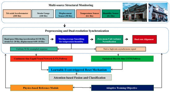
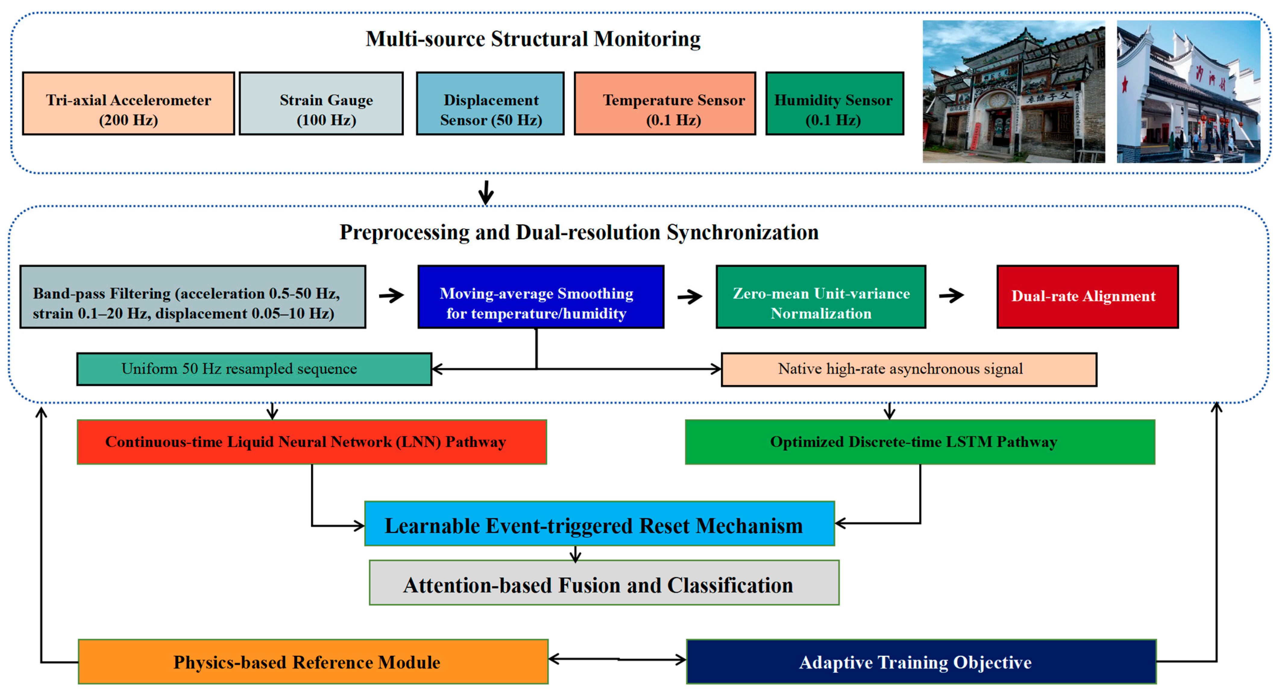
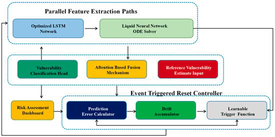
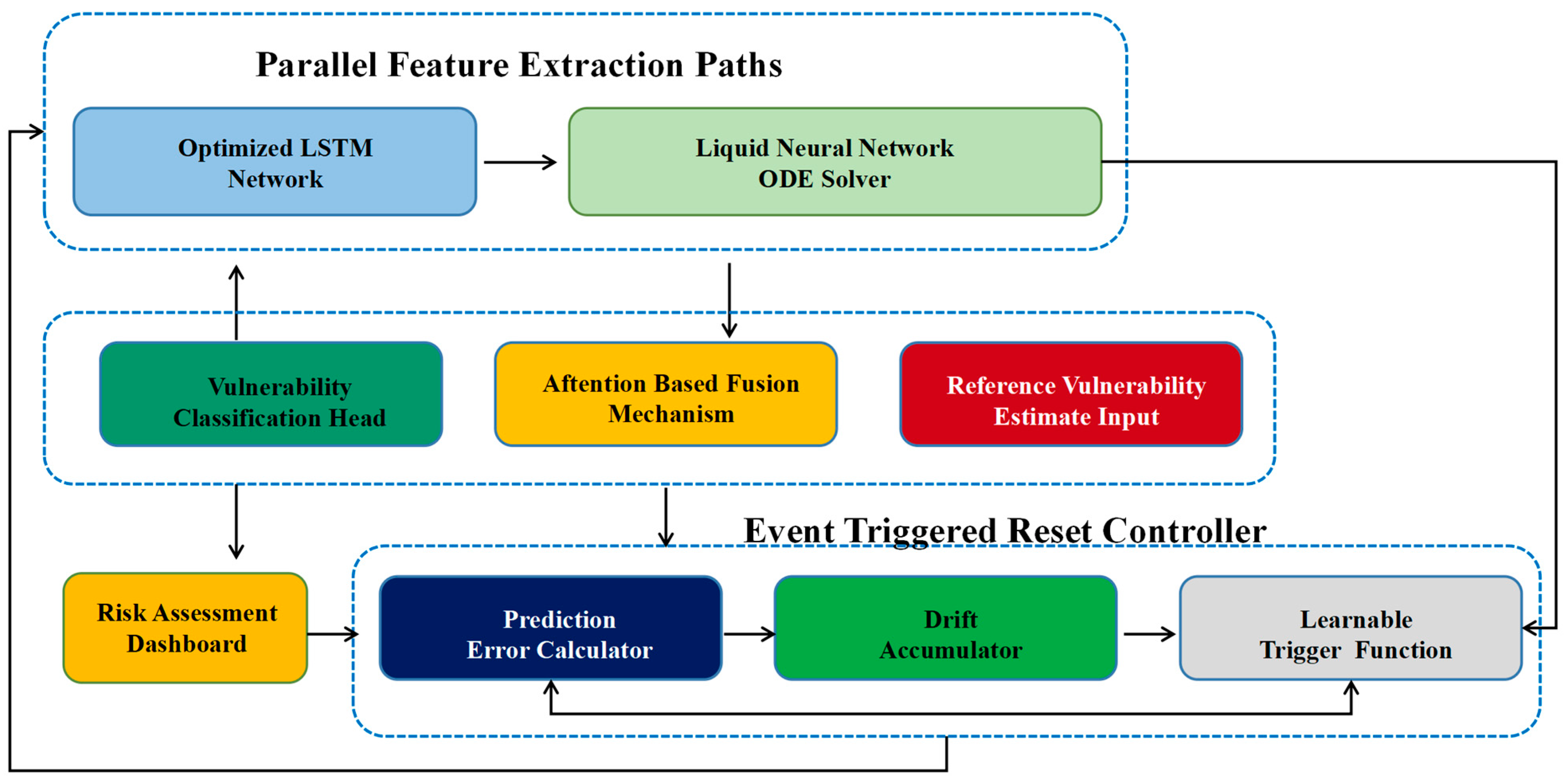
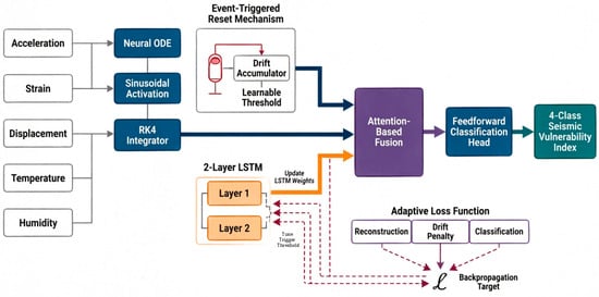
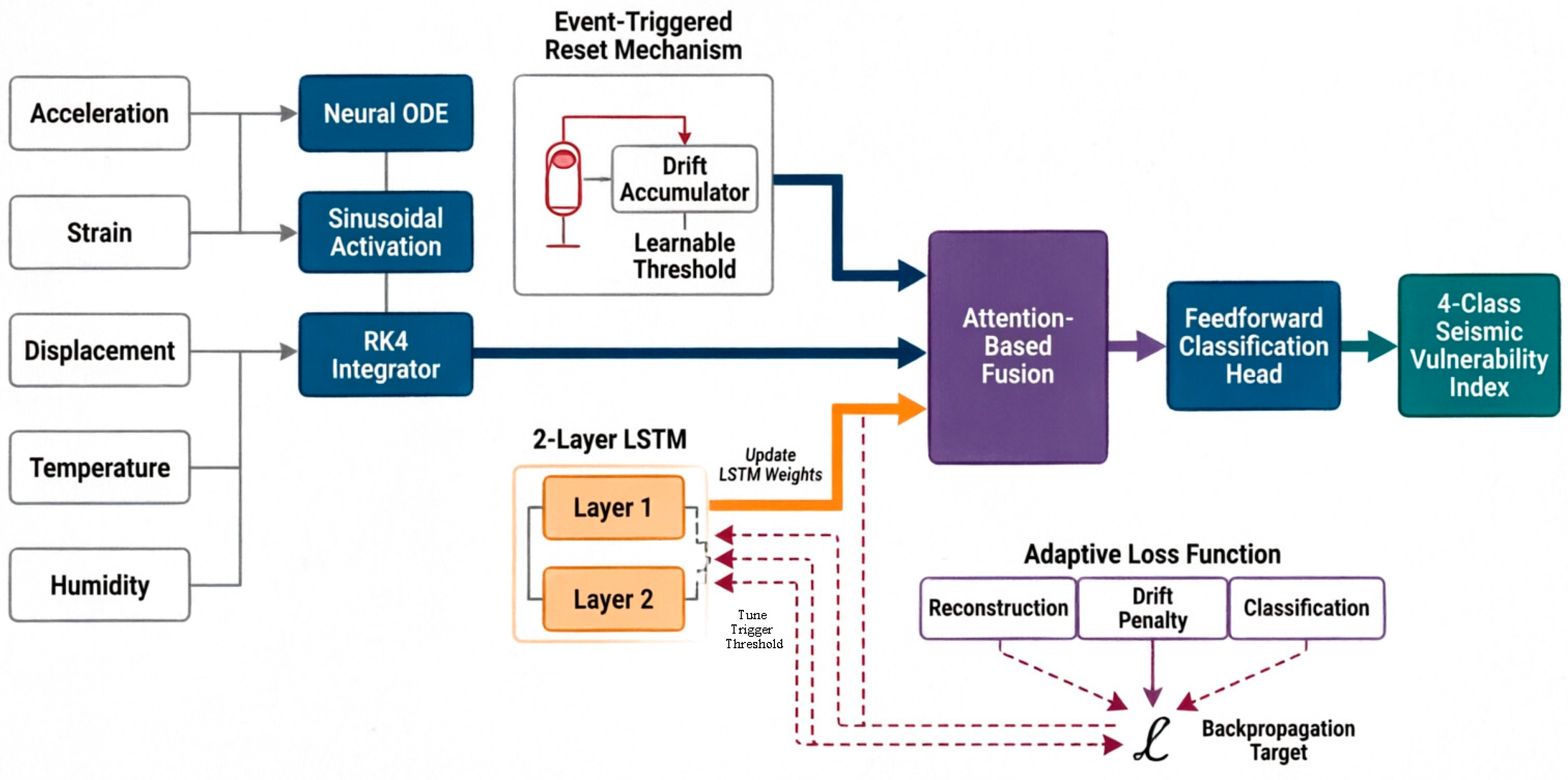
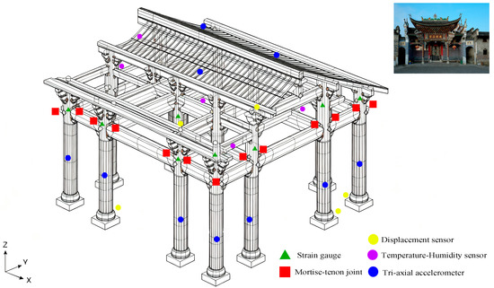
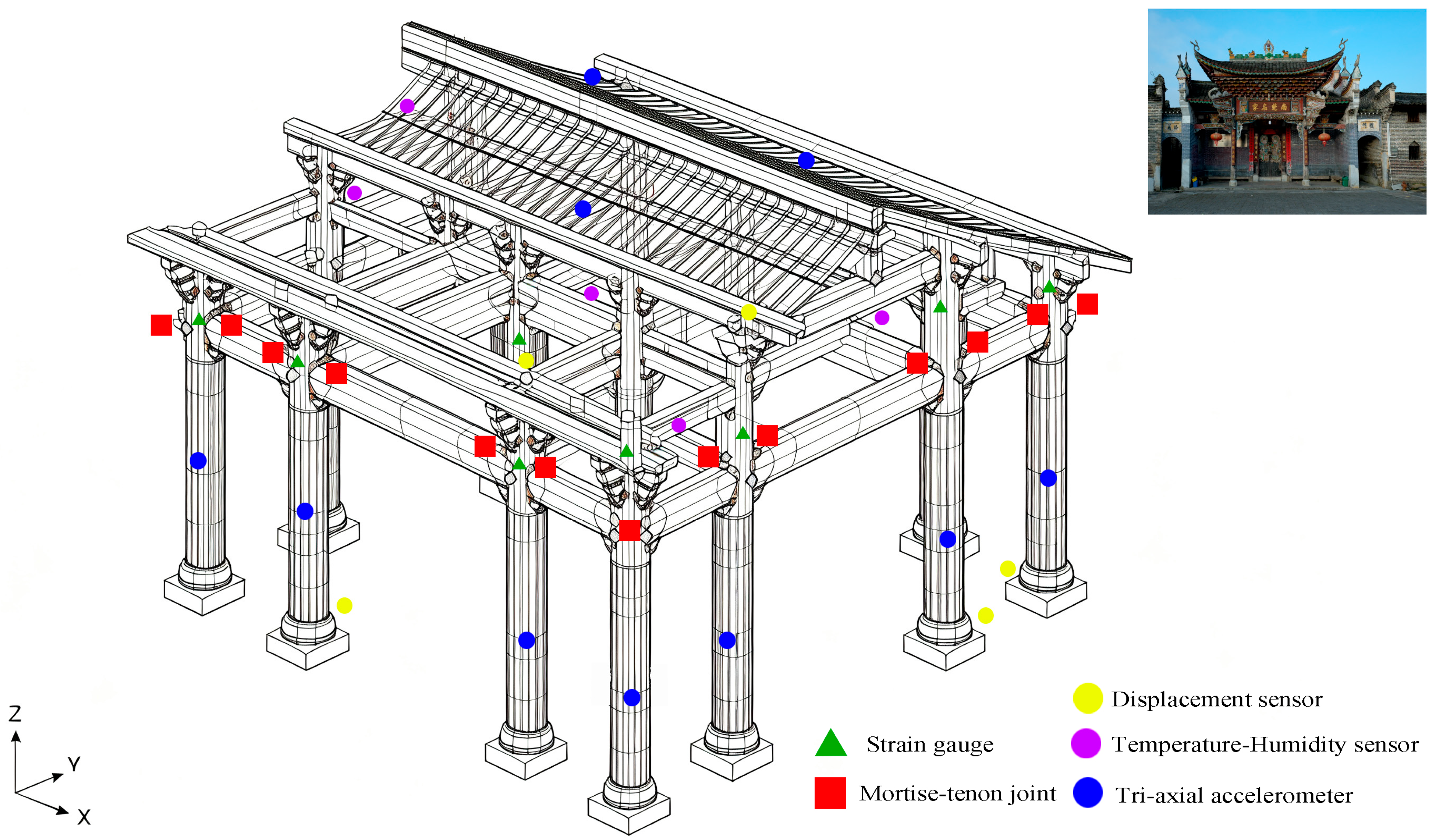
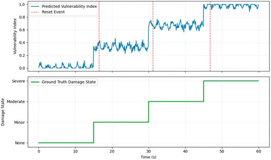
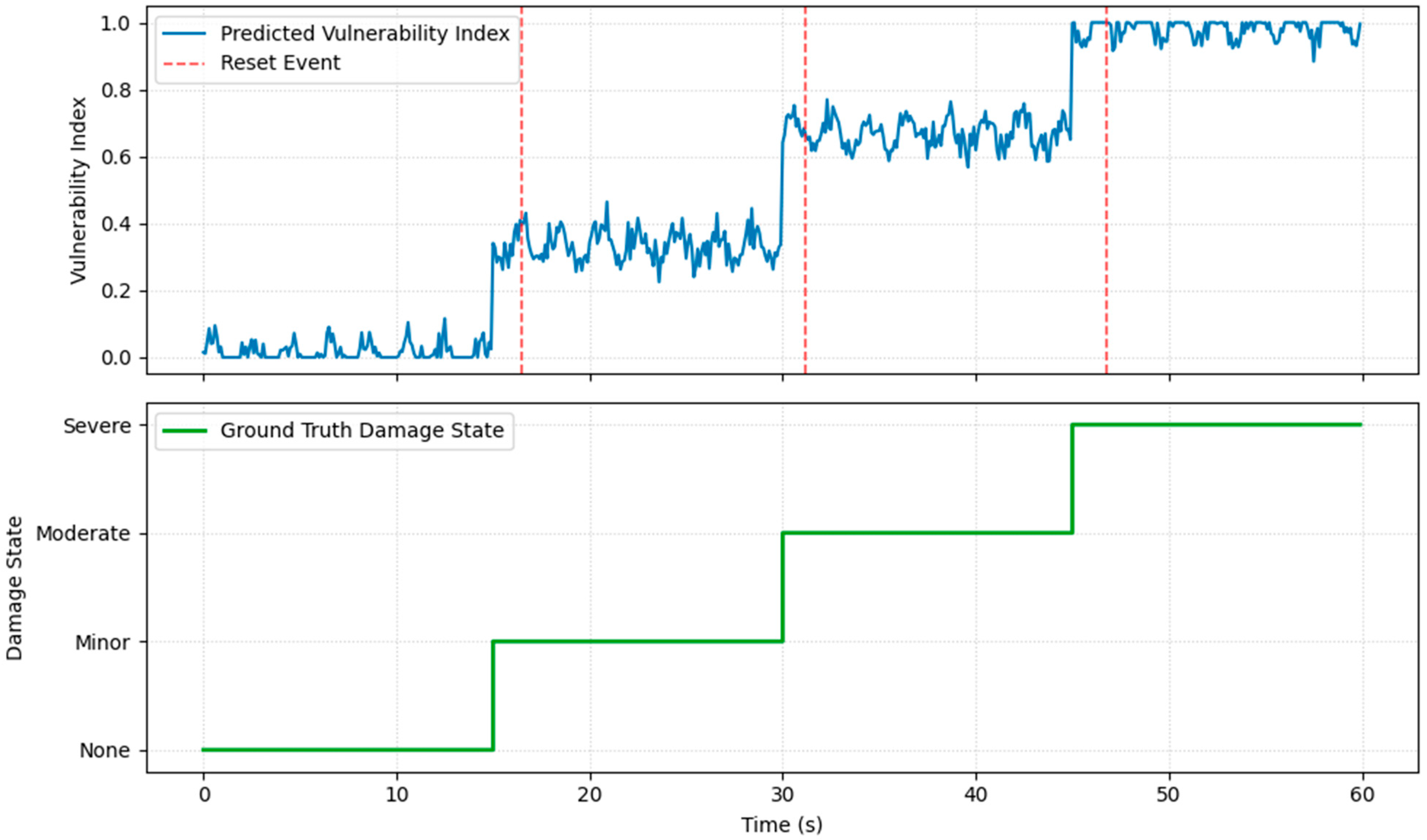
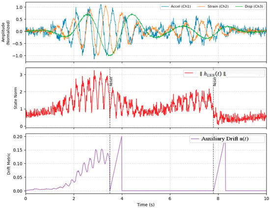
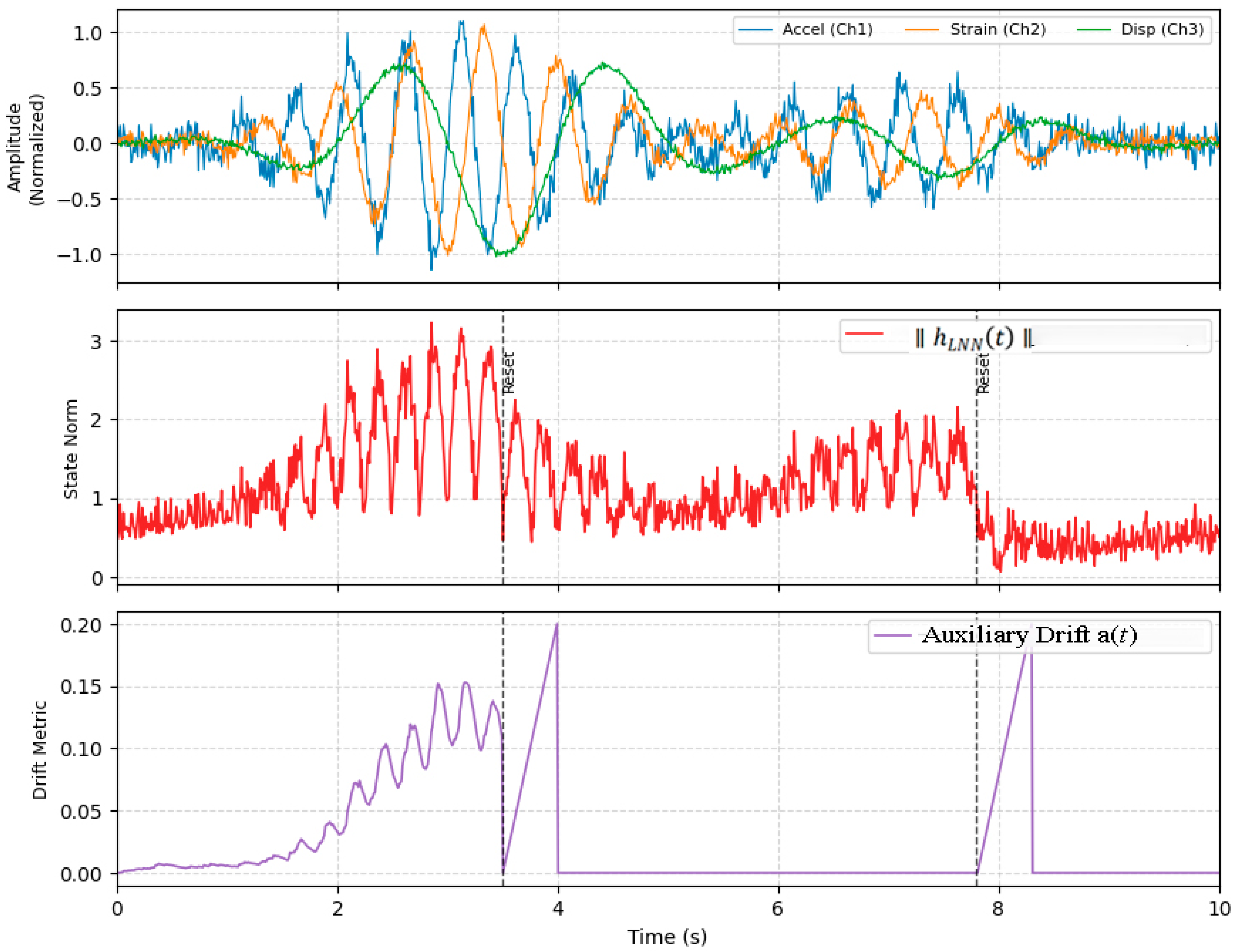

Disclaimer/Publisher’s Note: The statements, opinions and data contained in all publications are solely those of the individual author(s) and contributor(s) and not of MDPI and/or the editor(s). MDPI and/or the editor(s) disclaim responsibility for any injury to people or property resulting from any ideas, methods, instructions or products referred to in the content. |
© 2026 by the authors. Licensee MDPI, Basel, Switzerland. This article is an open access article distributed under the terms and conditions of the Creative Commons Attribution (CC BY) license.