


Abstract
To investigate the effects of model selection, time-varying parameters and climatic differences on the carbon emission reduction performance of rural rooftop photovoltaic (PV) systems, this study selected a typical rural residential rooftop PV system in Beijing as the research object. Hourly simulations using the System Advisor Model (SAM) and an operational-period baseline method were employed to optimize the PV array parameters and conduct a multi-factor analysis of carbon emission reductions. The results show that the first-year electricity generation was 15,902 kWh, corresponding to an annual carbon emission reduction of 12.60 tCO2. The carbon emission reduction estimates obtained using the three irradiance models differed, with a maximum deviation of 0.51 tCO2. When both PV module degradation and changes in the grid emission factor were considered, the cumulative carbon emission reduction decreased by 68.37 tCO2 relative to the ideal scenario. Moreover, the faster the grid transition speed, the lower the cumulative carbon emission reduction over the system’s operational period. In addition, extending the analysis from a single region to multiple regions revealed that the annual carbon emission reductions in representative rural residential rooftop PV systems in Beijing and Wuhan differed by 2.94 tCO2, with differences also observed in their seasonal variation patterns. The assessment of rural rooftop PV systems should comprehensively consider irradiance model selection, module power degradation, grid transition pathways, regional climatic conditions and economic feasibility.
1. Introduction
Accelerating global warming and persistently excessive greenhouse gas emissions constitute a critical environmental crisis confronting humanity [1]. In 2020, China explicitly announced its strategic goals of achieving carbon peaking before 2030 and carbon neutrality before 2060. The transition of the energy mix is a key pathway to achieving these goals [2]. Characterized by cleanliness, low-carbon performance and renewability, photovoltaic (PV) electricity generation has become one of the preferred technologies for advancing decarbonization within the energy sector [3].
However, land-resource constraints represent a significant challenge for large-scale PV development. Ground-mounted PV projects compete with other land-use types such as agricultural production and ecological conservation. Rooftop PV systems utilize existing building roofs without requiring additional land, thereby effectively alleviating conflicts between energy development and other land uses. Meanwhile, the electricity generated by PV systems can displace part of the grid-supplied electricity, thereby playing an important role in increasing renewable energy use in buildings and facilitating the low-carbon energy transition [4]. Rooftop PV has therefore become an important form of renewable energy deployment in both urban and rural built environments.
Current research on carbon emission reductions from rooftop PV systems primarily follows three pathways. These are spatial potential assessment, carbon emission reduction accounting and system simulation. For spatial potential identification, remote sensing and Geographic Information System (GIS) technologies have been widely applied to rooftop resource assessment. Studies at the global and national scales have revealed broad spatial patterns in the carbon-mitigation potential of PV systems [5], while studies at the urban and regional scales have evaluated the temporal development potential of rooftop resources [6,7]. However, these assessments generally rely on standardized parameters and therefore have difficulty capturing engineering constraints specific to rural rooftops, such as PV array layout and inter-row shading. For carbon emission reduction accounting, existing methods mainly include life-cycle assessment (LCA) and the baseline method. Because these methods adopt different system boundaries, their results are not directly comparable. LCA covers carbon emissions across the entire PV supply chain [8], whereas the baseline method quantifies the emission reduction benefits of PV generation displacing grid-supplied electricity during the operational period [9]. Existing studies are mostly based on static assumptions, treating PV electricity generation and the grid emission factor as constant values. Consequently, they do not adequately account for module performance degradation during the operational period or for variations in ambient temperature, which can accelerate module degradation and affect the system’s operational-period electricity generation capacity [10]. Bistline [11] further pointed out that failing to adequately account for the displacement of other electricity-generation sources by PV systems would lead to an overestimation of their emission-reduction benefits. In terms of system simulation, software tools such as the System Advisor Model (SAM, v2025.4.16, National Renewable Energy Laboratory, Golden, CO, USA) and PVsyst (v8.1.0, PVsyst SA, Satigny, Switzerland) are widely used to simulate PV electricity generation. Detailed simulations can reduce errors in carbon emission reduction assessments [12]. However, differences in model inputs and calculation methods across simulation platforms can affect the reliability of the results [13]. Most studies directly adopt the default diffuse irradiance model provided by the simulation software. Although previous studies have shown that tilted surface irradiance models affect estimates of PV electricity generation [14,15], few studies have quantified the propagation effect of such errors on carbon emission reduction outcomes. Furthermore, existing studies on carbon emission reductions from rooftop PV systems have primarily focused on urban settings or a single region. Comparative assessments of carbon emission reductions from rural rooftop PV systems across different regions remain limited, and the mechanisms through which climatic differences affect operational-period carbon emission reduction estimates have not been fully clarified.
Accordingly, this paper takes a rural rooftop PV system in Beijing as the research project and establishes an operational-period carbon emission reduction accounting model using SAM as the simulation platform and the baseline method. On this basis, three tilted surface diffuse irradiance models are first compared to quantify the systematic propagation of model selection errors into carbon emission reduction outcomes. Second, the analysis considers an ideal scenario, a module degradation scenario, a grid decarbonization scenario and a coupled scenario incorporating both module degradation and grid decarbonization. The independent and coupled effects of these two time-varying factors on cumulative carbon emission reductions over the operational period are then quantified. Emission reductions under different grid transition rates are further compared. Finally, the analysis is extended from a single region to multiple regions to identify regional differences in carbon emission reductions. This study provides methodological support for operational-period carbon emission reduction accounting of rooftop PV systems and offers a theoretical basis and reference for irradiance model selection, PV module degradation assessment, grid transition pathway analysis, the treatment of regional climatic differences and economic evaluation.
2. Methodology
2.1. Carbon Emission Reduction Accounting Based on the Baseline Methodology
In accordance with the Clean Development Mechanism (CDM) methodologies and the Intergovernmental Panel on Climate Change (IPCC) Guidelines for National Greenhouse Gas Inventories, this study adopts the baseline method to quantify carbon emission reductions from the PV system. The accounting framework encompasses the calculation of electricity generated by the PV system, the identification and establishment of the system baseline scenario, the definition of the system boundary and the calculation of carbon emission reductions.
In carbon emission reduction accounting, the electricity generated by the PV system provides the basis for determining the system’s emission reduction benefits during the operational period. Its estimation primarily involves three key parameters: installed PV capacity, peak sun hours and the system performance ratio. The PV installed capacity is defined as the sum of the peak power ratings of all modules in the PV array under standard test conditions. Peak sun hours are the equivalent time length converted from the total solar irradiation received on the tilted surface within a given period under the standard irradiance (1000 W/m2) and serve as a key simplified indicator for estimating the electricity generation of PV systems. The system performance ratio (PR) is a key dimensionless indicator that measures the actual energy output of a PV system relative to its theoretical output and comprehensively accounts for losses associated with temperature, soiling, module mismatch, wiring, inverter operation and other system factors.
It is assumed that the PV array configuration and system operating mode remain unchanged throughout the operational period. Based on the above parameters, the PV electricity-generation model is expressed in Equation (1) [16].
The combined margin emission factor is a key indicator of the carbon intensity of marginal electricity supplied by the grid and is calculated as the weighted average of the operating margin and build margin emission factors. For PV power generation systems, the operating margin emission factor is assigned a weight of 75%, while the build margin emission factor is assigned a weight of 25% [17]. Accordingly, the combined margin emission factor for the North China Power Grid in year y is given in Equation (2).
The carbon emission reductions achieved by the PV system are determined as the baseline emissions minus the sum of system emissions and leakage emissions. Accordingly, the carbon emission reduction in year y is expressed by Equation (3).
The system boundary comprises the spatial boundary, temporal boundary and carbon-accounting boundary. The spatial boundary encompasses the rooftop PV system and its point of grid connection, including the PV modules, mounting structures, inverter, Alternating Current (AC) and Direct Current (DC) cables, metering equipment and grid-connection equipment. The temporal boundary covers the system’s 25-year operational period. The carbon-accounting boundary is limited to the operational period of PV generation and quantifies the carbon emission reductions achieved by displacing grid-supplied electricity with PV electricity. Direct system emissions and leakage emissions are set to zero in accordance with the applicable methodology.
The baseline scenario assumes that, in the absence of the PV system, an amount of electricity equivalent to that generated by the PV system would be supplied by the North China Power Grid. Baseline emissions are calculated using the electricity generated by the PV system and the combined margin emission factor of the North China Power Grid, assuming a one-to-one correspondence between PV electricity generation and displaced grid electricity. PV curtailment, energy losses during battery charging and discharging and additional transmission and distribution losses caused by PV grid integration are not considered.
Therefore, the carbon emission reduction achieved by the PV system in year y is given in Equation (4).
2.2. Tilted Surface Diffuse Irradiance Models
The total solar irradiation incident on the tilted surface of the PV array consists of direct-beam, diffuse and ground-reflected components, as expressed in Equation (5).
To ensure the comparability of the results obtained from the three irradiance models, the meteorological data, PV array parameters, module efficiency, system performance ratio and the methods for calculating beam and ground-reflected irradiance are held constant, while only the tilted-surface diffuse irradiance model is varied. The ground albedo is assumed to be constant, and its seasonal variation is neglected. Shading from surrounding buildings and obstruction by local terrain are not considered.
The isotropic model assumes that diffuse irradiance is uniformly distributed across the sky dome. The diffuse irradiation received by the tilted surface therefore depends on the surface tilt angle and is given in Equation (6).
The Hay–Davies–Klucher–Reindl (HDKR) model extends the isotropic model by introducing an anisotropy index and accounting for both circumsolar diffuse radiation and horizon brightening. The diffuse irradiation received by the tilted surface is expressed in Equation (7).
The Perez model is based on a physical representation of the sky luminance distribution and decomposes diffuse radiation into three components: circumsolar radiation, horizon brightening and isotropic sky-dome radiation. These components are adjusted using the sky clearness and sky brightness parameters, as expressed in Equation (8).
The diffuse irradiation on tilted surfaces is calculated separately using the three diffuse radiation models, and the corresponding electricity generation is determined by Equation (9).
The carbon emission reductions calculated using the three diffuse irradiance models are expressed in Equation (10).
2.3. Dynamic Carbon Emission Reduction Accounting During the Operational Period of the PV System
PV modules undergo light-induced degradation and age-related degradation during operation, thereby affecting electricity generation and environmental performance over the operational period [18,19]. This study does not consider performance recovery caused by module replacement, capacity expansion, major system failures or special maintenance. It is assumed that inter-annual meteorological resources and other system losses remain at the typical year level. Based on the power degradation rates in the first and subsequent years, electricity generation in year y is given by Equation (11).
As the power generation mix evolves and grid decarbonization progresses, the carbon intensity of grid electricity generally declines, affecting the operational-period emission reduction benefits of PV systems [20,21]. Future drivers are assumed to follow their historical trends, without considering unexpected disruptions such as abrupt policy changes or large-scale, disruptive transformations in the power generation mix. Based on the historical time series of combined margin emission factors for the North China Power Grid from 2014 to 2024, this study employs log-linear regression to characterize their exponential trend, as expressed in Equation (12).
The regression results are presented in Equation (13).
Potential policy-driven acceleration or deceleration of grid decarbonization is not considered. The compound annual reduction rate is assumed to remain constant throughout the operational period. The compound annual reduction rate is defined by Equation (14).
Based on the 95% confidence interval of the regression coefficient, three pathways representing slow, baseline and rapid grid transitions are established to characterize the uncertainty in future changes in the grid emission factor. The lower bound of the confidence interval, the regression point estimate and the upper bound of the confidence interval are used to determine the compound annual reduction rates for the slow, baseline, and rapid grid transition pathways, respectively. Taking the 2024 combined margin emission factor as the baseline, the combined margin emission factor of the North China Power Grid in year y under pathway j follows a compound annual reduction trajectory, as expressed in Equation (15).
Therefore, the cumulative carbon emission reductions achieved by the PV system during its operational period are expressed in Equation (16).
2.4. Economic Feasibility Calculation
The villagers export all electricity generated by the PV system to the national grid to obtain revenue, which is calculated using Equation (17).
As for costs, the initial investment, the annual operational cost, the annual maintenance cost and the annual average equipment renewal cost are included. Accordingly, the costs are calculated using Equations (18) and (19).
The net present value (NPV) of the rooftop PV system is calculated using Equation (20).
r stands for the financial discount rate. The IRR is obtained by setting the NPV equal to zero and solving for r. Based on the current development of China’s PV industry, r is set at 8% [22].
The investment payback period (IRP) is given by Equation (21).
The Life Cycle Cost (LCC) is the sum of the initial investment and the present value of annual operating costs, while the Levelized Cost of Electricity (LCOE) is the ratio of the LCC to the present value of annual electricity generation, as expressed in Equations (22) and (23).
The carbon abatement cost (CAC) is defined as the ratio of the life-cycle cost to the cumulative carbon emission reductions over the operational period. It is calculated according to the net cost method, as expressed in Equation (24).
3. Data and Results Analysis
This study employs LONGi LR5-72HPH-545M monocrystalline silicon modules (LONGi Green Energy Technology Co., Ltd., Xi’an, China) and a GoodWe GEH7.6-1U-US20 single-phase grid-connected inverter (GoodWe Technologies Co., Ltd., Suzhou, China) as the system components. Meteorological data are obtained from the National Solar Radiation Database (NSRDB) integrated into SAM, and the Perez anisotropic model is used to calculate irradiation on the tilted surface. The building has a flat roof with an area of 75 m2. PV modules are densely arranged, and the array utilization ratio is 80%.
3.1. PV Array Parameter Optimization
3.1.1. PV Array Tilt Angle Optimization
The PV array tilt angle is the angle between the module plane and the horizontal plane. It affects the angle at which solar radiation strikes the module surface, thereby influencing the solar irradiation received by the tilted surface, electricity generation and carbon emission reductions. The capacity factor is the ratio of the actual electricity generated by a PV system to the theoretical electricity generation at its rated power over the same period and is used to evaluate the system’s electricity generation performance.
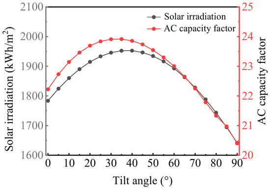
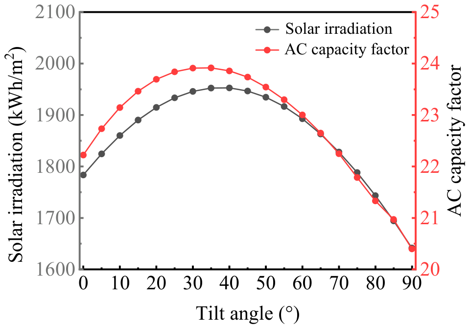
To determine the optimal tilt angle, annual tilted surface solar irradiation and the AC capacity factor are simulated for tilt angles ranging from 0° to 90°. The results are presented in Figure 1.
Figure 1.
Optimization simulation curve of PV array tilt angle.
As illustrated in Figure 1, both the annual total solar irradiation on the tilted surface and the AC capacity factor initially increase and then decrease as the PV array tilt angle increases. Within the range of 0°–30°, increasing the tilt angle improves the solar incidence geometry, resulting in a continuous increase in the solar irradiation received by the tilted surface and a corresponding increase in the system’s AC capacity factor. Within the range of 30°–40°, the annual total solar irradiation on the tilted surface and the AC capacity factor reach their respective maximum values. The optimal tilt angle for the AC capacity factor is slightly lower than that for annual irradiation, indicating that AC electricity-generation performance is not determined solely by the available solar resource. The different responses of module temperature, temperature-dependent conversion losses, inverter efficiency and other system losses to changes in tilt angle jointly contribute to the offset between the two peaks.
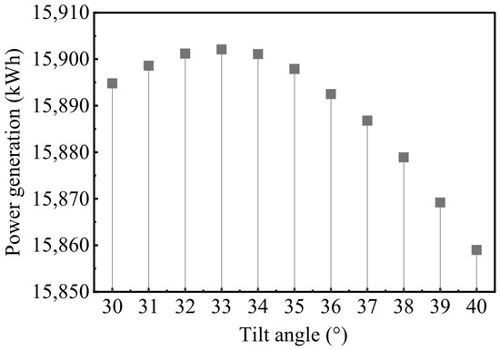
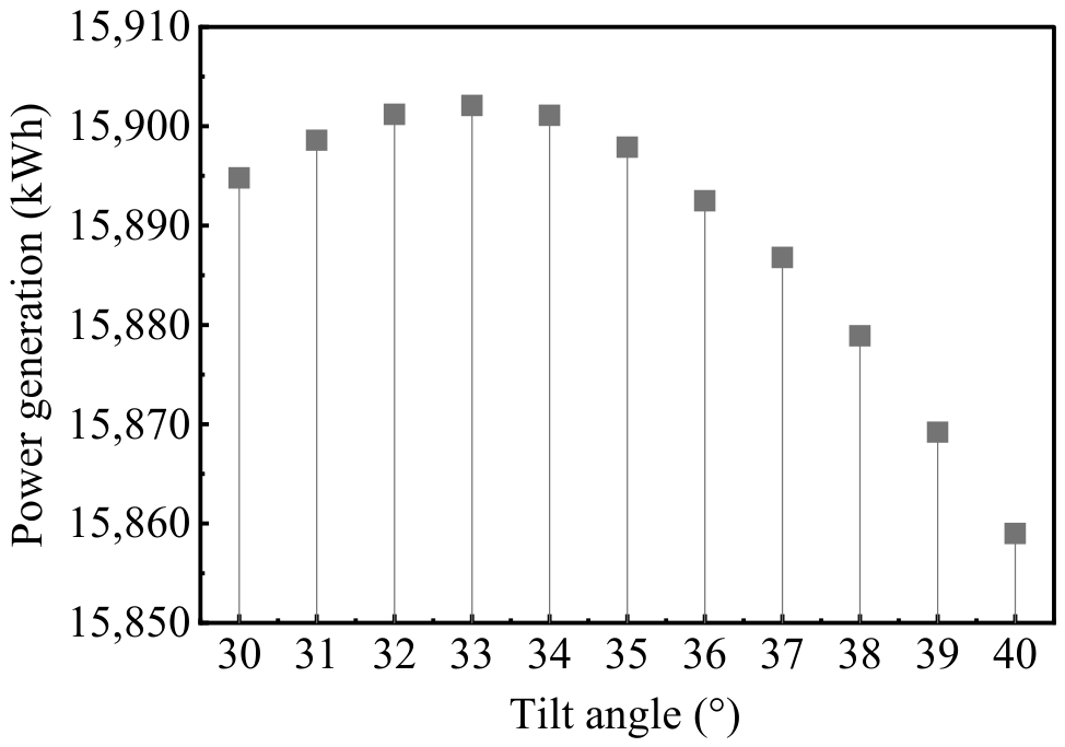
To maximize carbon emission reductions, this study uses maximum annual electricity generation as the design objective and performs system simulations for tilt angles ranging from 30° to 40°. The results are presented in Figure 2.
Figure 2.
Annual electricity generation at tilt angles ranging from 30° to 40°.
As shown in Figure 2, annual electricity generation initially increases and then decreases with the tilt angle. Grid-connected AC electricity generation reaches its maximum at a tilt angle of 33° and decreases progressively beyond this angle. Therefore, 33° is selected as the optimal tilt angle for the PV system.
3.1.2. Ground Coverage Ratio and Inter-Row Spacing Optimization
The ground coverage ratio (GCR) is the ratio of the horizontal projected area of the PV array to the land area occupied by the array. It is a key dimensionless parameter characterizing the spacing and density of the array layout.
The GCR depends on the module length along the tilted surface, L, the installation tilt angle, β, and the horizontal clear spacing between the bases of adjacent rows, D. Variations in mounting structure height are neglected. These parameters satisfy the following geometric relationship, as expressed in Equation (25).
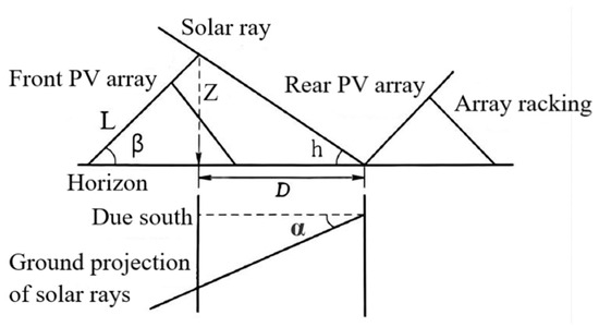
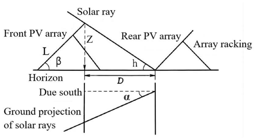
As shown in Equation (25), the GCR is inversely related to the inter-row spacing. A higher GCR indicates a smaller row spacing and greater rooftop-area utilization but also increases inter-row shading losses. Therefore, the inter-row spacing should be determined based on the shading conditions. The geometric relationship governing inter-row shading in the PV array is illustrated in Figure 3.
Figure 3.
Geometric schematic of PV array layout spacing.
Based on the geometric relationship presented in Figure 3, the PV array inter-row spacing is jointly determined by the vertical height difference between the highest point of the front row and the base of the rear row, the solar altitude angle and the solar azimuth angle. The shadow-length multiplier is defined as the product of the cotangent of the solar altitude angle and the cosine of the solar azimuth angle. This geometric shadow-spacing calculation assumes parallel incident solar rays, a flat horizontal ground surface and neglects external shading from surrounding objects. Accordingly, the inter-row spacing is expressed in Equation (26).
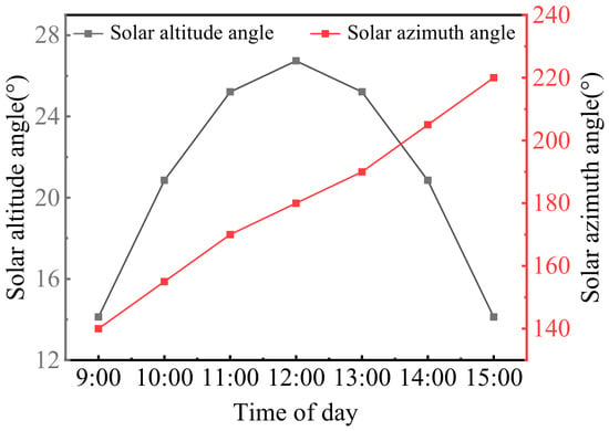
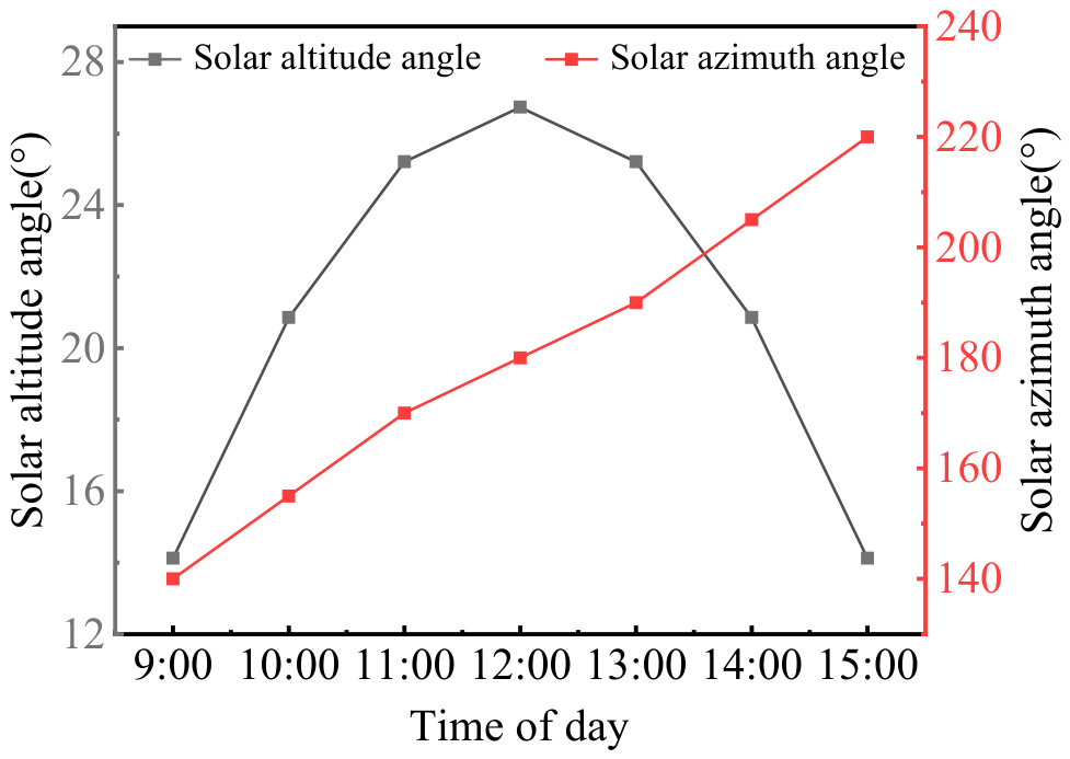
The no-shading condition on the winter solstice determines the theoretical upper limit of the GCR. If the GCR exceeds this limit, inter-row shading will inevitably occur on the winter solstice, with shading losses increasing rapidly as the GCR increases. Therefore, a no-shading requirement throughout the period from 9:00 to 15:00 on the winter solstice is imposed as a design constraint. The hourly solar altitude and azimuth angles during this period are extracted, as shown in Figure 4, to determine the minimum array row spacing and subsequently calculate the maximum GCR.
Figure 4.
Hourly solar altitude and azimuth angles on the winter solstice.
The calculated minimum inter-row spacing is 2.53 m, corresponding to a maximum GCR of 0.25. A total of 18 PV modules are installed on the roof in a three-row by six-column configuration. The array rows extend from east to west, and the modules are tilted toward the south. The overall array dimensions are 8.216 m in the north–south direction and 7.26 m in the east–west direction, resulting in an actual rooftop footprint of 59.6 m2.
3.2. Electricity Generation Performance and System Losses
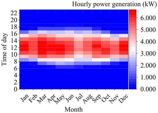
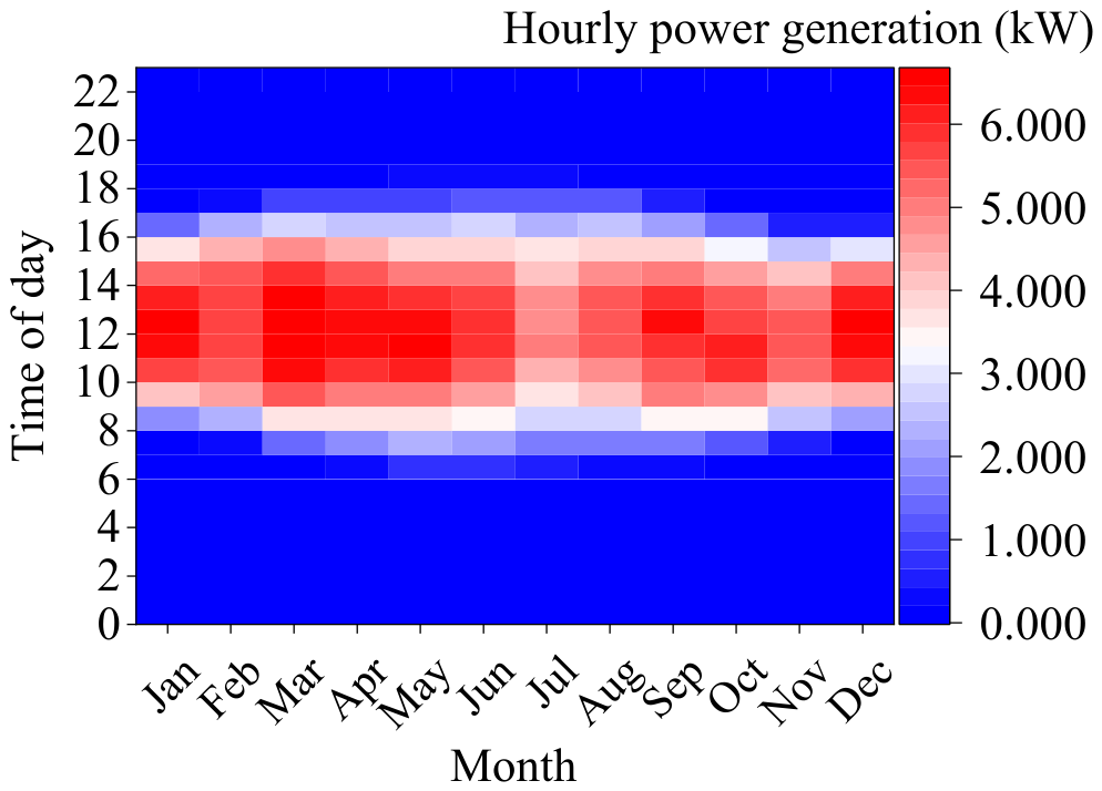
A heatmap showing hourly electricity generation for all 8760 h of the year is generated from the simulation results and presented in Figure 5. The horizontal axis represents the day of the year, while the vertical axis represents the time of day. The color scale indicates the power output at each time step, revealing the temporal distribution of PV generation across diurnal and seasonal scales.
Figure 5.
Heatmap of hourly PV electricity generation throughout the year.
Figure 5 presents the hourly distribution of PV power output throughout the year. Regarding the diurnal variation, electricity generation is mainly concentrated between 7:00 and 17:00, with high power output generally occurring from 10:00 to 15:00. Solar irradiance is relatively high around noon, and the system power output generally reaches high daily levels. In contrast, lower solar irradiance in the early morning and late afternoon results in a corresponding decrease in power output.
Regarding seasonal variations, spring exhibits favorable solar resource conditions, with high-power-output regions covering a relatively large portion of the heatmap. Although summer has longer daylight hours, increased cloud cover during the rainy season and reduced conversion efficiency caused by elevated module temperatures result in lower system power output than in spring. In winter, shorter daylight hours, lower solar altitude angles, and greater angle-of-incidence losses substantially shorten the effective generation period and reduce overall electricity generation. Annual electricity generation exhibits a clear seasonal pattern, with higher output in spring and summer and lower output in autumn and winter. March records the highest monthly electricity generation at 1580 kWh, whereas November records the lowest at 1054.27 kWh.
In addition, losses during energy conversion and transmission affect electricity generation. To clarify how the net AC electricity generation is derived, this study further analyzes the energy losses at each stage. The overall system losses mainly occur during solar irradiance capture, DC electricity generation, inverter conversion and AC electricity output. The nominal solar energy incident on the array surface is 87,423 kWh. After accounting for irradiance-capture losses caused by inter-row shading, soiling and angle-of-incidence reflection, the nominal DC electricity generation is 18,093 kWh. After further accounting for losses associated with deviations of actual module operating conditions from standard test conditions, module mismatch, diodes and connections and DC wiring, the net DC electricity generation is 17,011 kWh. Additional losses occur during inverter conversion because of conversion inefficiency, power clipping, inverter self-consumption and nighttime standby consumption, resulting in gross AC electricity generation of 16,182 kWh. After accounting for AC wiring losses and the subhourly clipping correction, the net AC electricity exported to the grid is 15,902 kWh.
3.3. Carbon Emission Reduction Accounting and Environmental Benefit Assessment
To quantify carbon emission reductions during the operational period of the PV system, this study adopts the 2024 Baseline Emission Factors for China’s Regional Power Grids for Emission Reduction Projects, published by the National Center for Climate Change Strategy and International Cooperation under the Ministry of Ecology and Environment of China. According to the report, the 2024 operating margin emission factor for the North China Power Grid is 0.0009531 tCO2/kWh, while the build margin emission factor is 0.0003095 tCO2/kWh. The combined margin emission factor is calculated using Equation (2), and the resulting expression is presented in Equation (27).
The monthly carbon emission reductions achieved by the PV system are expressed in Equation (28).
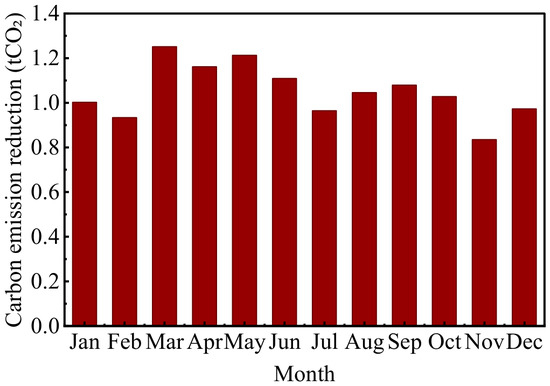
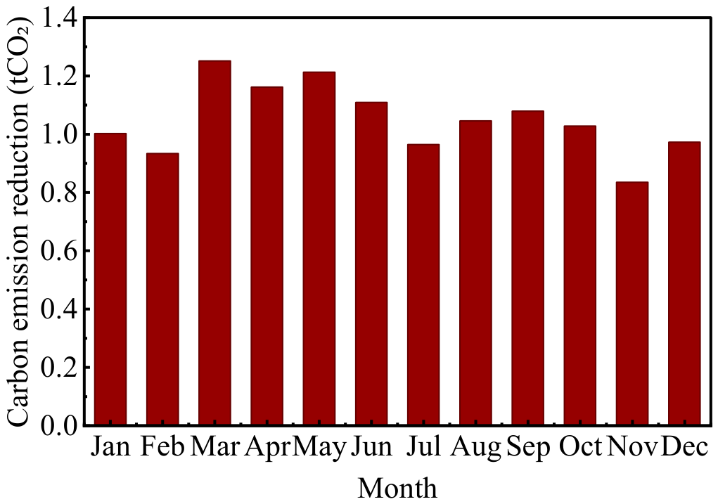
Electricity generation is aggregated by month and combined with the combined margin emission factor to calculate monthly carbon emission reductions, as shown in Figure 6.
Figure 6.
Monthly carbon emission reductions achieved by the PV system.
As shown in Figure 6, the monthly carbon emission reductions exhibit pronounced seasonal variations, with a trend broadly consistent with that of monthly electricity generation. The system can achieve an annual carbon emission reduction of 12.60 tCO2.
In terms of environmental benefits, based on the latest Annual Development Report of China’s Electric Power Industry, the annual PV electricity generation of 15,902 kWh can reduce standard coal consumption by approximately 4.81 tons of coal equivalent and avoid approximately 0.21 kg of particulate matter, 1.22 kg of sulfur dioxide and 1.99 kg of nitrogen oxide emissions.
3.4. Analysis of Factors Affecting Carbon Emission Reduction Accounting
3.4.1. Effects of Three Irradiance Models on Carbon Emission Reduction
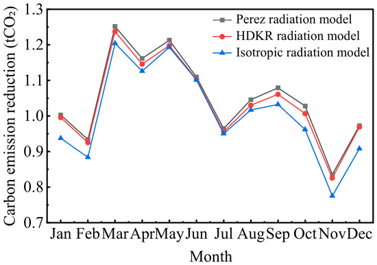
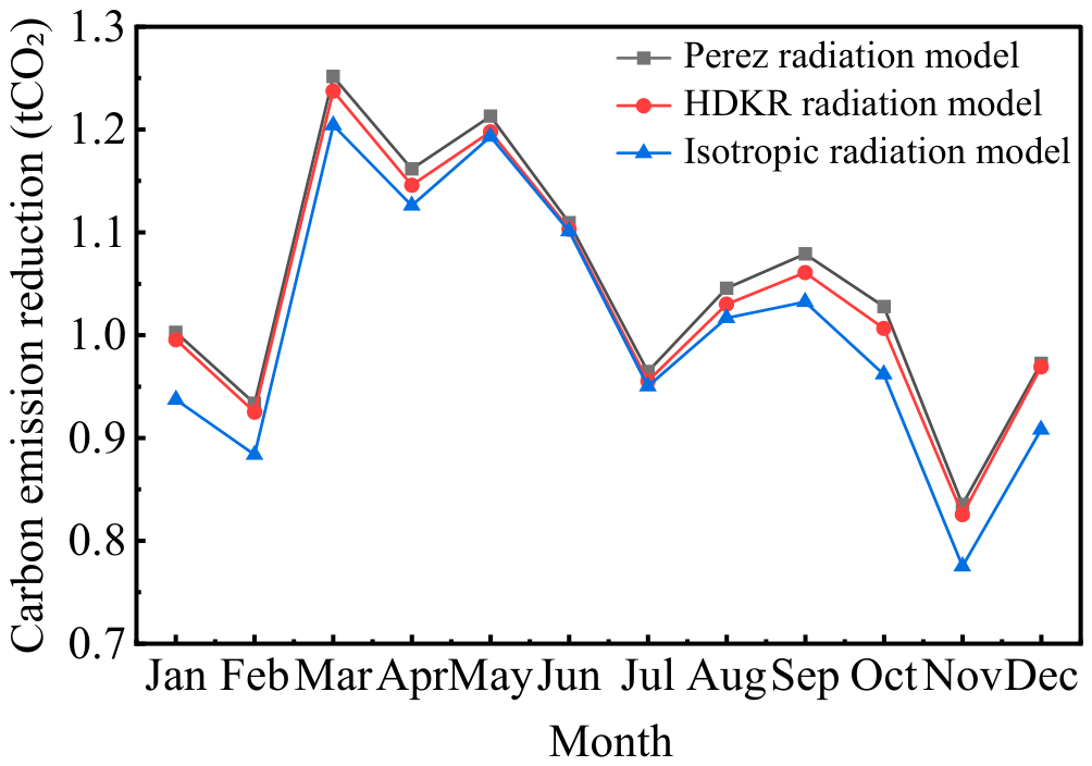
To evaluate the transmission effect of tilted surface diffuse irradiance model selection on carbon emission reduction accounting results, this section applies a controlled-variable approach. The PV array area, PV conversion efficiency, performance ratio and other parameters are held constant, while only the method used to calculate diffuse irradiation on the tilted surface is varied. Monthly electricity generation is first calculated using the isotropic, HDKR and Perez models, and the corresponding carbon emission reductions are then derived. The results are presented in Figure 7.
Figure 7.
Carbon emission reduction comparison among various radiation models.
As shown in Figure 7, all three models exhibit a seasonal pattern of higher carbon emission reductions in spring and summer and lower reductions in autumn and winter. However, differences exist in their numerical results. The annual carbon emission reductions calculated using the Perez, HDKR and isotropic models are 12.60, 12.45 and 12.09 tCO2, respectively. The maximum difference in first-year carbon emission reductions among the three models is 0.51 tCO2, which accounts for 4.05% of the result obtained from the Perez model. This result indicates that irradiance-model selection can lead to discrepancies in carbon emission reduction accounting.
The results show that, although the irradiance model is not a direct parameter in the carbon emission reduction accounting equation, it indirectly affects the accounting results by altering tilted surface irradiation and PV electricity generation. At present, the differences in carbon emission reductions among the three models are relatively small. However, these differences may continue to widen as grid decarbonization progresses and PV generation technologies advance, thereby exerting an increasingly significant influence on carbon emission reduction results.
3.4.2. Comparative Analysis of Carbon Emission Reductions Across Multiple Cities
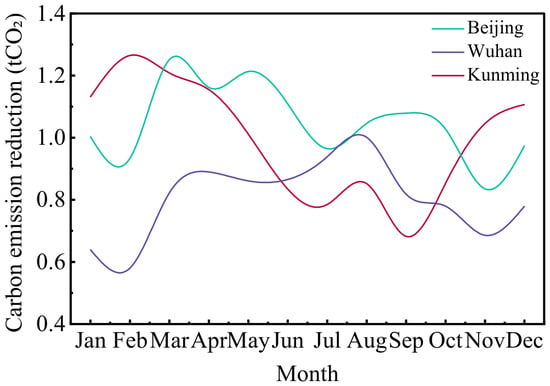
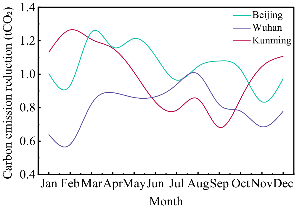
To investigate the effects of climatic differences on operational-period carbon emission reductions from rural rooftop PV systems, this section applies a controlled-variable approach. The installed capacity, array tilt angle, azimuth angle and other design parameters are held constant, while three representative cities, namely Beijing, Wuhan and Kunming, are selected for comparison. Figure 8 shows the variation patterns in carbon emission reductions achieved by a representative rural rooftop PV system in each city.
Figure 8.
Comparison of carbon emission reductions from representative rural rooftop PV systems across multiple cities.
As shown in Figure 8, annual carbon emission reductions differ substantially among the three regions. The annual reductions in Beijing, Wuhan and Kunming are 12.60, 9.66 and 11.93 tCO2, respectively. The maximum difference is 2.94 tCO2 and is mainly attributable to regional meteorological conditions. In Beijing, abundant solar irradiation and moderate temperatures in spring result in relatively high PV conversion efficiency and corresponding increases in carbon emission reductions. In winter, limited solar resources lead to a substantial decline in emission reductions. Wuhan experiences frequent cloudy and rainy weather, resulting in a relatively uniform monthly distribution of solar irradiation and smaller fluctuations in monthly carbon emission reductions. In Kunming, frequent cloudy weather during summer and autumn limits beam irradiation, whereas predominantly clear conditions in winter and spring result in higher carbon emission reductions during these seasons.
The results indicate that the carbon emission reduction accounting analytical methods developed for the Beijing case can provide a reference for other rural regions. When assessing carbon emission reductions from rural rooftop PV systems across different regions, meteorological, system and grid parameters specific to the system location should be adopted, together with a localized analysis of climatic and environmental conditions, to improve the regional applicability and reliability of the accounting results.
3.4.3. Scenario Analysis of PV Module Degradation and Grid Transition
Over the 25-year operational period of the PV system, module power degradation causes electricity generation to decline annually, thereby indirectly reducing carbon emission reductions. Variations in the regional grid emission factor also exert an influence on carbon emission reduction outcomes of the PV system. Therefore, PV module power degradation and changes in the grid emission factor are two time-varying factors influencing the system’s carbon emission reductions.
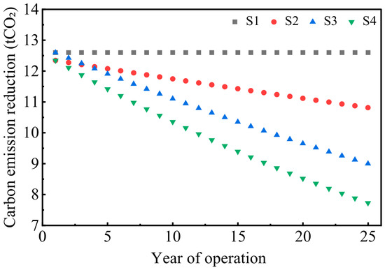
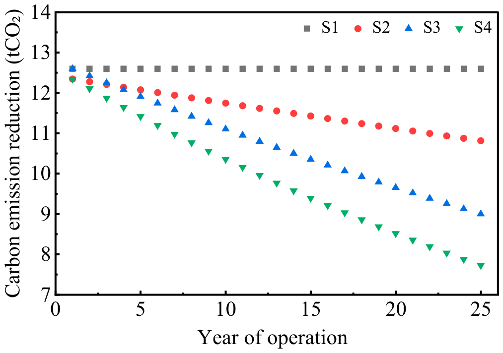
To investigate the independent and joint effects of these two factors, this section applies a controlled-variable approach and establishes four scenarios under identical conditions. S1 represents the ideal scenario, in which both electricity generation and the grid emission factor remain constant. S2 represents the module degradation scenario and considers only PV module power degradation, with electricity generation declining annually while the grid emission factor remains constant. S3 represents the grid decarbonization scenario and considers only the decline in the grid emission factor, while electricity generation remains constant. S4 represents the coupled scenario incorporating both factors and considers both PV module power degradation and the decline in the grid emission factor.
Based on the performance parameters of the LR5-72HPH-545M module, the first-year power degradation rate is set to 2%, followed by an annual degradation rate of 0.55% in subsequent years. Figure 9 shows the annual carbon emission reductions achieved by the rural rooftop PV system in Beijing over its 25-year operational period under the four scenarios.
Figure 9.
Annual carbon emission reduction during the operational period under four scenarios.
As shown in Figure 9, cumulative carbon emission reductions across the four scenarios range from 243.81 to 314.94 tCO2, with a range of 71.13 tCO2. Under S1, the annual carbon emission reduction remains constant at 12.60 tCO2 throughout the operational period. Under S2, it gradually decreases from 12.35 tCO2 in the first year to 10.82 tCO2 in year 25. Under S3, it decreases from 12.60 tCO2 in the first year to 9.00 tCO2 at the end of the operational period. Under S4, it declines from 12.35 to 7.72 tCO2 over the same period.
During the first three years of PV system operation, annual carbon emission reductions under S3 are higher than those under S2. From year 4 onward, the reductions under S3 remain lower than those under S2. This indicates that the impact of power-grid decarbonization on emission-reduction benefits exceeds that of module degradation and becomes the dominant factor in the middle-to-late stage of the operational period. Furthermore, considering either PV module degradation or the decline in the grid emission factor alone substantially affects the estimated operational-period carbon emission reductions. Therefore, both time-varying parameters should be incorporated into a dynamic accounting model to avoid biases arising from static assumptions.
However, PV module power degradation is affected by factors such as manufacturing processes, encapsulation materials, operating conditions and aging mechanisms. To examine the effects of variations in degradation parameters on carbon emission reductions over the operational period, three module degradation scenarios—low, baseline and high degradation—were established. Their first-year and subsequent annual degradation rates were set at 1.0% and 0.30%, 2.0% and 0.55% and 3.0% and 0.80%, respectively. Without considering module replacement or performance recovery, the cumulative electricity generation over the 25-year operational period under the three scenarios was 379,726.39, 364,937.67 and 350,777.56 kWh, respectively.
In addition to module degradation, changes in the future grid emission factor represent another source of uncertainty in carbon emission reduction estimates. Therefore, based on the coupled scenario S4, three grid transition pathways—slow, baseline and rapid—were established, with compound annual reduction rates of the grid emission factor of 0.865%, 1.392% and 1.917%, respectively. The three module degradation scenarios were combined with the three grid transition pathways to construct nine joint scenarios, as presented in Table 1.
Table 1.
Cumulative carbon emission reductions over the operational period under different module degradation scenarios and grid transition pathways (unit: tCO2).
Across the nine joint scenarios, the cumulative carbon emission reductions over the 25-year operational period ranged from 224.23 to 271.94 tCO2, corresponding to deviations of −9.06% to +10.29% from the baseline combination value of 246.57 tCO2. The low-degradation–slow-transition combination produced the highest cumulative carbon emission reduction, whereas the high-degradation–rapid-transition combination produced the lowest. This indicates that variations in module degradation parameters and grid transition rates jointly broaden the range of estimated carbon emission reductions over the operational period. These findings are consistent with the results of the S1–S4 scenario analysis. In addition, under all parameter combinations, the cumulative carbon emission reductions over the 25-year operational period were lower than the 314.94 tCO2 estimated under the ideal scenario S1.
3.5. Economic Feasibility Analysis
To evaluate the practical applicability of the rooftop PV system, an economic feasibility analysis was conducted for the technically optimized configuration described above. The system consists of 18 PV modules, each with a rated power of 545 W, resulting in a total installed capacity of 9.81 kWp. The equipment and installation costs are 3.0 and 0.5 RMB/W, respectively, corresponding to an initial investment of CNY 34,335.00. The annual operating, maintenance and average equipment renewal costs are assumed to be 0.04%, 0.032% and 0.32% of the initial investment, respectively [23].
The system operates under a full-grid-export mode, with a feed-in tariff of 0.3598 RMB/kWh. Considering a first-year module degradation rate of 2% and an annual degradation rate of 0.55% thereafter, the cumulative electricity generation over the 25-year operational period is 364,937.67 kWh, corresponding to an undiscounted electricity sales revenue of CNY 131,304.57. The main economic evaluation results are presented in Table 2.
Table 2.
Economic evaluation results of the rooftop PV system.
As shown in Table 2, at a financial discount rate of 8%, the project has a life cycle cost of CNY 35,771.75 and a levelized cost of electricity of CNY 0.2249/kWh, which is lower than the baseline feed-in tariff of CNY 0.3598/kWh, indicating that the system has a certain cost advantage in electricity generation.
The project has a discounted payback period of 9.34 years, which is shorter than the 25-year operational period. Its net present value is CNY 21,465.92, and its internal rate of return is 14.95%, exceeding the benchmark discount rate of 8%. These results demonstrate that the project is financially feasible under the specified economic assumptions. Based on the cumulative carbon emission reduction of 246.57 tCO2 over the 25-year operational period under scenario S4, the net carbon abatement cost is CNY −87.06/tCO2 after deducting the present value of electricity sales revenue. The negative value indicates that the project can generate positive net economic returns while delivering carbon emission reduction benefits.
3.6. Limitations
This study has several limitations. First, owing to the lack of comparable operational monitoring data from rural rooftop PV systems, the assessments of electricity generation, carbon emission reductions and economic performance are primarily based on SAM simulations and have not yet been validated against measured data. Second, the conclusions regarding the optimal tilt angle, GCR, inter-row spacing, electricity generation and carbon emission reductions are mainly applicable to the flat-roof rural residence considered in this study and may not be directly transferable to other roof geometries or rural housing typologies. Future research will collect hourly and monthly operational data from actual systems and conduct parametric and field-based analyses of different rural housing types, roof geometries, array layouts and system capacities. These efforts will facilitate model calibration, clarify the applicability of the optimization results and improve the reliability and generalizability of the carbon emission reduction and economic assessments.
4. Conclusions
This study investigates a rural residential rooftop PV system in Beijing. Carbon emission reductions are analyzed using SAM simulations and the operational-period baseline accounting method, and the main conclusions are summarized as follows:
- (1)
- The PV array optimization results indicate an optimal tilt angle of 33°, a minimum inter-row spacing of 2.53 m and a maximum ground coverage ratio of 0.25. Under this configuration, the system generates 15,902 kWh of electricity, corresponding to a carbon emission reduction of 12.60 tCO2.
- (2)
- The difference in annual carbon emission reductions between the Perez and isotropic models is 0.51 tCO2, indicating that irradiance model selection introduces differences into carbon emission reduction results. This difference accumulates over the system’s operational period. Therefore, the irradiance model adopted should be explicitly specified in the accounting process.
- (3)
- The cumulative carbon emission reductions under the S1 ideal scenario and the S4 coupled scenario incorporating both factors are 314.94 tCO2 and 246.57 tCO2, respectively. This difference indicates that neglecting PV module power degradation and dynamic changes in the grid emission factor leads to an overestimation of emission reduction benefits during the system’s operational period. Therefore, both parameters that vary over time should be incorporated into carbon emission reduction accounting. Slow, baseline and rapid grid transition pathways should also be considered to determine a reasonable range of cumulative carbon emission reductions.
- (4)
- Extending the analysis from a single region to multiple regions reveals a difference of 2.94 tCO2 in annual carbon emission reductions between Beijing and Wuhan. This result indicates that climatic differences affect carbon emission reduction results for rural rooftop PV systems and that location-specific parameters should be adopted for targeted analysis.
Author Contributions
Conceptualization, W.S. and S.Q.; methodology, W.S. and S.Q.; software, S.Q.; validation, W.S. and S.Q.; formal analysis, W.S. and S.Q.; investigation, W.S. and S.Q.; resources, W.S.; data curation, S.Q.; writing—original draft preparation, S.Q.; writing—review and editing, W.S.; visualization, W.S.; supervision, W.S.; project administration, W.S.; funding acquisition, W.S. All authors have read and agreed to the published version of the manuscript.
Funding
This research was funded by the Third Set of Endorsed Projects under the International Decade of Sciences for Sustainable Development (No. 19). The APC was funded by the authors.
Data Availability Statement
The original contributions presented in this study are included in the article. Further inquiries can be directed to the corresponding author.
Acknowledgments
This study is sponsored by Third Set of Endorsed Projects under the International Decade of Sciences for Sustainable Development (No. 19).
Conflicts of Interest
The authors declare no conflicts of interest.
Nomenclature
| E | Electricity generation of the PV system (kWh) |
| Rated installed capacity of PV system (kWp) | |
| Peak sun hours (h) | |
| Grid emission factor (tCO2/kWh) | |
| C | Carbon emission reduction (tCO2) |
| Solar irradiation (kWh/m2) | |
| PV module tilt angle (°) | |
| Anisotropy index | |
| Beam irradiance geometric factor | |
| Horizon brightening correction factor | |
| Perez coefficient | |
| Perez coefficient | |
| a | Solar geometry parameters |
| b | Solar geometry parameters |
| ε | Sky clearness parameter |
| Δ | Sky brightness parameter |
| PV panel area (m2) | |
| PV module power degradation rate | |
| PV conversion efficiency | |
| Intercept | |
| Annual logarithmic change coefficient of the emission factor | |
| n | Calendar year |
| Random error term | |
| Compound annual reduction rate | |
| j | Grid transition pathway identifier |
| L | PV module length along the tilted surface (m) |
| D | Horizontal clear spacing between the bases of adjacent PV array rows (m) |
| h | Solar altitude angle |
| Solar azimuth angle | |
| R | Shadow-length multiplier |
| Vertical height difference between the highest point and the base of the PV array (m) | |
| The quantity of electricity sold to the grid | |
| The annual electricity sales revenue from the rooftop PV system | |
| The on-grid electricity price | |
| The capital investment per unit installed capacity of PV | |
| The installation cost per unit installed capacity of PV | |
| Initial investment cost | |
| Expenditure | |
| Operational cost | |
| Maintenance cost | |
| Equipment renewal cost | |
| Subscript | |
| y | System Operating Year |
| BL | Baseline |
| e | Emission |
| l | Leakage |
| T | Tilted surface |
| t | total |
| b | Beam |
| r | Reflection |
| d | Diffuse |
| Irradiance Model Identifier | |
| m | Month |
| Combined Margin | |
| OM | Operating Margin |
| Build Margin | |
References
- IPCC. Climate Change 2023: Synthesis Report. Contribution of Working Groups I, II and III to the Sixth Assessment Report of the Intergovernmental Panel on Climate Change; IPCC: Geneva, Switzerland, 2023. [Google Scholar]
- Zhang, X.; Huang, X.; Zhang, D.; Geng, Y.; Tian, L.; Fan, Y.; Chen, W. Research on the Pathway and Policies for China’s Energy and Economy Transformation toward Carbon Neutrality. J. Manag. World 2022, 38, 35–66. [Google Scholar]
- Zhang, Z.; Qian, Z.; Chen, M.; Zhu, R.; Zhang, F.; Zhong, T.; Lin, J.; Ning, L.; Xie, W.; Creutzig, F.; et al. Worldwide rooftop photovoltaic electricity generation may mitigate global warming. Nat. Clim. Change 2025, 15, 393–402. [Google Scholar] [CrossRef] [Scilit]
- Yao, H.; Zhou, Q. Research status and application of rooftop photovoltaic generation systems. Clean. Energy Syst. 2023, 5, 100065. [Google Scholar] [CrossRef] [Scilit]
- Zhang, Z.; Chen, M.; Zhong, T.; Zhu, R.; Qian, Z.; Zhang, F.; Yang, Y.; Zhang, K.; Santi, P.; Wang, K.; et al. Carbon mitigation potential afforded by rooftop photovoltaic in China. Nat. Commun. 2023, 14, 2347. [Google Scholar] [CrossRef] [Scilit]
- Xu, W.; Wang, P. Assessment of rooftop photovoltaic power generation potential and environmental benefits in urban central districts under different climatic conditions. J. Environ. Eng. Technol. 2025, 15, 1502–1512. [Google Scholar]
- Miao, S.; Huang, Y.; Zhang, X. Study on the Prediction and Effect of Carbon Emission Reduction Potential of Rooftop Photovoltaic Systems in Wuhu City. Urban. Archit. 2025, 18, 79–81. [Google Scholar]
- Dong, L.; Gu, Y.; Cai, K.; He, X.; Song, Q.; Yuan, W.; Duan, H. Unveiling lifecycle carbon emissions and its mitigation potentials of distributed photovoltaic power through two typical case systems. Sol. Energy 2024, 269, 112360. [Google Scholar] [CrossRef] [Scilit]
- Niu, S. The Research of Project Level Carbon Emissions Problems on Roof Photovoltaic Grid-Connected Power Generation Project. Master’s Thesis, Hebei University of Engineering, Han Dan, China, 2014. [Google Scholar]
- Poddar, S.; Rougieux, F.; Evans, J.P.; Kay, M.; Prasad, A.A.; Bremner, S.P. Accelerated degradation of photovoltaic modules under a future warmer climate. Prog. Photovolt. Res. Appl. 2024, 32, 456–467. [Google Scholar] [CrossRef] [Scilit]
- Bistline, J.E.T.; Watten, A. Emissions reductions of rooftop solar are overstated by approaches that inadequately capture substitution effects. Nat. Clim. Change 2025, 15, 1173–1175. [Google Scholar] [CrossRef] [Scilit]
- Olivieri, L.; Caamaño-Martín, E.; Sassenou, L.N.; Olivieri, F. Contribution of photovoltaic distributed generation to the transition towards an emission-free supply to university campus: Technical, economic feasibility and carbon emission reduction at the Universidad Politécnica de Madrid. Renew. Energy 2020, 162, 1703–1714. [Google Scholar] [CrossRef] [Scilit]
- Kaleshwarwar, A.; Bahadure, S. Validating the credibility of solar simulation tools using a real-world case study. Energy Build. 2023, 301, 113697. [Google Scholar] [CrossRef] [Scilit]
- Dubois, A.M.; Bourdin, V.; Torres Aguilar, M.I.; Bonnassieux, Y. Estimation of the uncertainty due to each step of simulating the photovoltaic conversion under real operating conditions. Int. J. Photoenergy 2021, 2021, 4228658. [Google Scholar] [CrossRef] [Scilit]
- Prilliman, M.J.; Hansen, C.W.; Keith, J.M.F.; Janzou, S.; Theristis, M.; Scheiner, A.; Ozakyol, E. Quantifying Uncertainty in PV Energy Estimates: Final Report; NREL/TP–7A40–84993; National Renewable Energy Laboratory: Golden, CO, USA, 2023. [Google Scholar]
- GB 50797-2012; Code for Design of Photovoltaic Power Station. China Planning Press: Beijing, China, 2012.
- United Nations Framework Convention on Climate Change. Tool to Calculate the Emission Factor for an Electricity System, Version 07.0 (TOOL07); UNFCCC: Bonn, Germany, 2018. [Google Scholar]
- Nordin, A.H.M.; Sulaiman, S.I.; Shaari, S. Life cycle impact of photovoltaic module degradation on energy and environmental metrics. Energy Rep. 2022, 8, 923–931. [Google Scholar] [CrossRef] [Scilit]
- Aghaei, M.; Fairbrother, A.; Gok, A.; Ahmad, S.; Kazim, S.; Lobato, K.; Oreski, G.; Reinders, A.; Schmitz, J.; Theelen, M.; et al. Review of degradation and failure phenomena in photovoltaic modules. Renew. Sustain. Energy Rev. 2022, 159, 112160. [Google Scholar] [CrossRef] [Scilit]
- Gagnon, P.; Cole, W. Planning for the evolution of the electric grid with a long-run marginal emission rate. iScience 2022, 25, 103915. [Google Scholar] [CrossRef] [Scilit]
- Chen, S.; Lu, X.; Nielsen, C.P.; McElroy, M.B.; He, G.; Zhang, S.; He, K.; Yang, X.; Zhang, F.; Hao, J. Deploying solar photovoltaic energy first in carbon-intensive regions brings gigatons more carbon mitigations to 2060. Commun. Earth Environ. 2023, 4, 369. [Google Scholar] [CrossRef] [Scilit]
- Zhang, Y.; He, H.; Huang, J.; Li, H. Economic benefit analysis of rail transit photovoltaic power generation and energy storage integration project based on levelized net present value model. Urban Mass Transit 2023, 26, 103–108. [Google Scholar]
- Wang, M.; Mao, X.; Gao, Y.; He, F. Potential of carbon emission reduction and financial feasibility of urban rooftop photovoltaic power generation in Beijing. J. Clean. Prod. 2018, 203, 1119–1131. [Google Scholar] [CrossRef] [Scilit]

Disclaimer/Publisher’s Note: The statements, opinions and data contained in all publications are solely those of the individual author(s) and contributor(s) and not of MDPI and/or the editor(s). MDPI and/or the editor(s) disclaim responsibility for any injury to people or property resulting from any ideas, methods, instructions or products referred to in the content. |
© 2026 by the authors. Licensee MDPI, Basel, Switzerland. This article is an open access article distributed under the terms and conditions of the Creative Commons Attribution (CC BY) license.