Interpretable Machine Learning Framework for Predicting Air Void Content in Sustainable Steel-Slag SMA Mixtures Using Metaheuristic-Optimized XGBoost

Abstract

Air void content (Va) is a key volumetric parameter governing the performance of Stone Mastic Asphalt (SMA), yet its prediction becomes challenging when steel slag, fibers, and additives are incorporated. This study develops an interpretable machine learning framework for predicting Va using 74 mixtures collected from 16 published studies and nine mixture-related variables. XGBoost was optimized using Particle Swarm Optimization and Grey Wolf Optimizer (GWO), with the best configuration obtained by GWO at a population size of 40 and a minimum development-stage 5-fold cross-validation (CV) RMSE of 0.371%. On the principal 70/30 evaluation partition, the optimized model achieved R² = 0.944, RMSE = 0.397%, MAE = 0.262%, and MAPE = 0.054, outperforming the evaluated benchmark models in R², RMSE, MAE, and MAPE. Robustness analyses showed that prediction accuracy was sensitive to data partitioning and literature-source composition, indicating that the reported performance should be interpreted within the represented data domain. SHAP, permutation importance, and feature-ablation analyses consistently identified binder penetration as the most influential predictor, followed mainly by asphalt content and softening point. Overall, the proposed framework provides an interpretable tool for preliminary Va estimation and mixture screening, while independent laboratory and field validation remains necessary before practical deployment.

1. Introduction

The global road construction sector is currently facing dual challenges: the depletion of natural aggregate sources and the increasing demand for pavement systems capable of withstanding heavier traffic loads and harsher climatic conditions [1,2,3]. These challenges are driving a paradigm shift toward sustainable and circular engineering solutions. The adoption of circular economy principles in pavement engineering, particularly through the use of industrial by-products as alternative materials, has emerged as a key strategy to reduce environmental impacts and enhance resource efficiency. By reutilizing industrial waste streams, the construction industry not only conserves virgin resources but also addresses issues related to waste management, thereby contributing to a more sustainable future for infrastructure development.

The use of Stone Mastic Asphalt (SMA) mixtures incorporating steel slag aggregates simultaneously addresses the dual challenges of meeting pavement structural requirements and advancing sustainable, circular engineering solutions. SMA is a gap-graded asphalt mixture characterized by a stone-on-stone aggregate skeleton and a rich mortar of binder and filler [4]. This unique structure provides SMA with outstanding properties, particularly its superior resistance to rutting and high durability, making it a preferred choice for pavement layers subjected to heavy traffic loads. The use of steel slag as an alternative aggregate to natural stone has gained significant attention due to its mechanical and environmental benefits. Steel slag offers high angularity and excellent abrasion resistance while promoting the reutilization of industrial by-products [5,6,7,8]. However, when steel slag is incorporated into SMA, issues related to volumetric stability, particularly the residual air void content (Va), may become critical. Within gap-graded SMA, the Va functions as the principal metric for evaluating stone-on-stone skeletal integrity. Variations in Va resulting from slag absorption or fiber interference negatively affect the resistance of the mixture to permanent deformation and fatigue cracking. Consequently, accurate volumetric forecasting is necessary to establish adequate structural performance [9,10].

Because SMA typically contains a high asphalt binder content, fiber additives such as cellulose, basalt, polypropylene, or ceramic fibers are incorporated to prevent binder drain down [11,12,13,14]. Beyond this primary function, fibers also contribute to reinforcing the internal structure of the SMA mixture. Each fiber type, ranging from organic cellulose to mineral basalt, possesses distinct morphological characteristics that alter the binder–matrix interface. When combined with the vesicular, porous structure of steel slag, these additives create highly non-linear volumetric interactions that defy traditional empirical modeling, necessitating the use of advanced ensemble learning techniques like XGBoost to capture these complex dependencies.

Conventional measurement of Va can be affected by heterogeneity in steel slag, including variations in porosity, angularity, and material source. These sources of variability motivate the complementary use of data-driven methods to examine nonlinear relationships among mixture constituents and volumetric properties. Data-driven models provide a complementary means of examining nonlinear relationships between mixture composition and volumetric response. In this context, machine learning (ML) has increasingly been applied to asphalt-material prediction problems, including moisture susceptibility [15], dynamic modulus [16], skid resistance [17], and cracking resistance through the CTindex parameter [18]; these models often treat aggregate properties as homogeneous variables. Existing analytical approaches frequently lack the capacity to account for the stochastic variability and chemo-physical complexity inherent to steel slag. Characteristics such as elevated internal porosity and a known susceptibility to volumetric expansion produce considerable uncertainty regarding binder absorption and the resulting effective Va. The interaction of these material properties generates a highly non-linear parameter space that conventional empirical equations and standard ML architectures are typically unable to accurately resolve. Consequently, there is a critical need for an optimized, interpretable framework that can map the synergistic effects of various fibers and slag substitution rates on SMA volumetrics.

Recent asphalt and pavement studies have increasingly complemented predictive machine learning models with post hoc interpretation. Kongkitkul et al. [19] applied explainable artificial intelligence to asphalt-concrete stiffness and rutting-resistance prediction. Vargas and El Hanandeh [20] used SHAP with literature-derived asphalt-mixture data to examine both global and local contributions of mixture variables to several properties, including Va. At the pavement-performance scale, Sandamal et al. [21] combined supervised ML with explainable analysis for long-term pavement roughness prediction. These studies demonstrate the increasing use of feature-attribution methods to examine how fitted models use material and pavement variables. However, interpretability methods characterize specific aspects of model behavior and should not, by themselves, be treated as evidence of physical causality [22].

In this study, an XGBoost model was developed to predict the residual Va content of SMA mixtures incorporating steel slag aggregates and different fiber and additive systems. PSO and GWO were employed to investigate the four selected XGBoost hyperparameters, and the resulting configuration was evaluated using a principal training-testing partition together with additional sensitivity analyses addressing data partitioning, source-study composition, and categorical encoding. Moreover, repeated train-test partitioning and source-study sensitivity analyses were conducted to examine the dependence of predictive performance on sample allocation and literature-source composition, together with comparisons against conventional ML models. Finally, global and local SHAP analyses were complemented by permutation-based and feature-ablation analyses to examine the stability of the principal model attributions. Accordingly, the contribution of the present work lies not in proposing a new ML algorithm, but in integrating prediction, metaheuristic model development, robustness assessment, comparative evaluation, and multi-method interpretation for the specific problem of Va prediction in literature-derived steel-slag SMA data.

2. Database Description and Analysis

The database plays a crucial role in training and validating ML models. In this study, the dataset used to develop the ML model for predicting the Va of SMA mixtures incorporating steel slag aggregates was compiled from 16 publications in reputable scientific journals. These publications are directly related to SMA mixtures utilizing steel slag as a partial replacement for natural aggregates at various substitution rates and incorporating different types of fiber additives. The collected dataset consists of 74 samples (Table 1), structured with nine input variables selected based on their theoretically and experimentally established influence on the volumetric properties of steel-slag SMA mixtures. These inputs include fiber-related characteristics, fiber type (X1) and fiber content (X2, %); characteristics of other additives, additive type (X3) and additive content (X4, %); binder properties, penetration (X5, 0.1 mm), softening point (X6, °C), and asphalt content (X7, %); and steel slag aggregate parameters, replaced aggregate type (X8) and the steel slag replacement ratio (X9, %). The steel slag replacement ratio (X9) quantifies the proportion of natural aggregate substituted with steel slag, consisting primarily of Electric Arc Furnace (EAF) and Basic Oxygen Furnace (BOF) materials. This replacement spans the complete substitution spectrum (0–100%), reflecting the mixture proportions documented in the primary experimental literature. The sole dependent variable, which serves as the prediction target, is the Va.

Table 1. Data from experiments published in the relevant literature.

No.	Reference	Number of Samples	No.	Reference	Number of Samples
1	Wu et al. [23]	2	2	Shao-peng et al. [24]	1
3	Alinezhad and Sahaf [25]	4	4	Pasetto and Baldo [26]	2
5	Chen et al. [27]	4	6	Djakfar and Arifin [28]	6
7	Zhao et al. [29]	2	8	Shen et al. [30]	4
9	Cui et al. [31]	6	10	Cao et al. [32]	4
11	Wang et al. [33]	5	12	Rajesh et al. [34]	12
13	Wan et al. [35]	8	14	Zhang et al. [36]	5
15	Moazami et al. [37]	8	16	Xue et al. [38]	1
Total					74

Only observations reporting the complete set of nine input variables together with measured Va were retained. Additional candidate observations with incomplete reporting for one or more of these variables were not incorporated because their inclusion would require missing-data imputation or modification of the defined predictor space. Consequently, the 74 observations from the 16 publications in Table 1 represent the maximum complete dataset retained for the nine-variable model specification adopted in this study. The limited sample size is therefore treated as a study boundary and is examined further through partition- and source-based sensitivity analyses.

The data preprocessing and encoding procedures were executed according to the specifications outlined in Table 2. Three categorical input variables, fiber type (X1), additive type (X3), and replaced aggregate type (X8), are nominal categorical variables and were represented by integer codes in the primary model. This representation preserves the original nine-variable input space and avoids the feature-space expansion associated with one-hot encoding in the present small dataset [39]. The numerical codes in Table 2 are category labels rather than physically ordered quantities. Because integer coding may nevertheless introduce artificial ordering into tree-based splits, the influence of categorical representation was examined separately using one-hot encoding and XGBoost native categorical handling, as described in Section 3.6 and evaluated in Section 4.2.3.

Table 2. Description and numerical coding of categorical input variables.

Variable X1		Variable X3		Variable X8
Type of Fiber	Code	Type of Another Additive	Code	Type of Aggregate Replaced	Code
No fiber used	1	No other additives used	1	No use of steel slag	1
Rock wool	2	Sasobit	2	Coarse aggregate	2
Polyester	3	Ca(OH)2	3	Fine aggregate	3
Bamboo	4	Steel fiber	4	Coarse and fine aggregate	4
Basalt	5	Particle PET	5	All aggregates	5
Lignin	6	Ceramic	6
PET	7
Cellulose	8

Table 3 presents a statistical overview of the dataset variables. The descriptive statistics include the mean, standard deviation (std), minimum and maximum values, as well as the median. These computed statistics characterize the central tendency, variability, and general distribution patterns of each variable within the dataset.

Table 3. The inputs and outputs of the dataset are used to develop ML models.

Features	Type	Mean	Std	Min	Median	Max
Fiber type—X1	Input	4.51	2.36	1.00	4.00	8.00
Fiber content—X2 (%)	Input	0.25	0.12	0.00	0.30	0.40
Additive type—X3	Input	1.82	1.49	1.00	1.00	6.00
Additive content—X4 (%)	Input	0.20	0.59	0.00	0.00	3.00
Penetration—X5 (0.1 mm)	Input	57.31	6.69	46.00	58.50	65.00
Softening point—X6 (°C)	Input	69.38	13.82	49.00	65.20	86.90
Asphalt content—X7 (%)	Input	6.13	0.51	4.00	6.20	7.00
Replaced aggregate type—X8	Input	1.88	0.81	1.00	2.00	5.00
Replacement ratio—X9 (%)	Input	38.57	29.50	0.00	53.30	100.00
Va (%)	Output	4.49	1.47	2.91	4.00	10.54

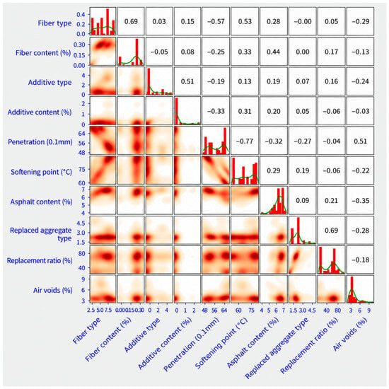
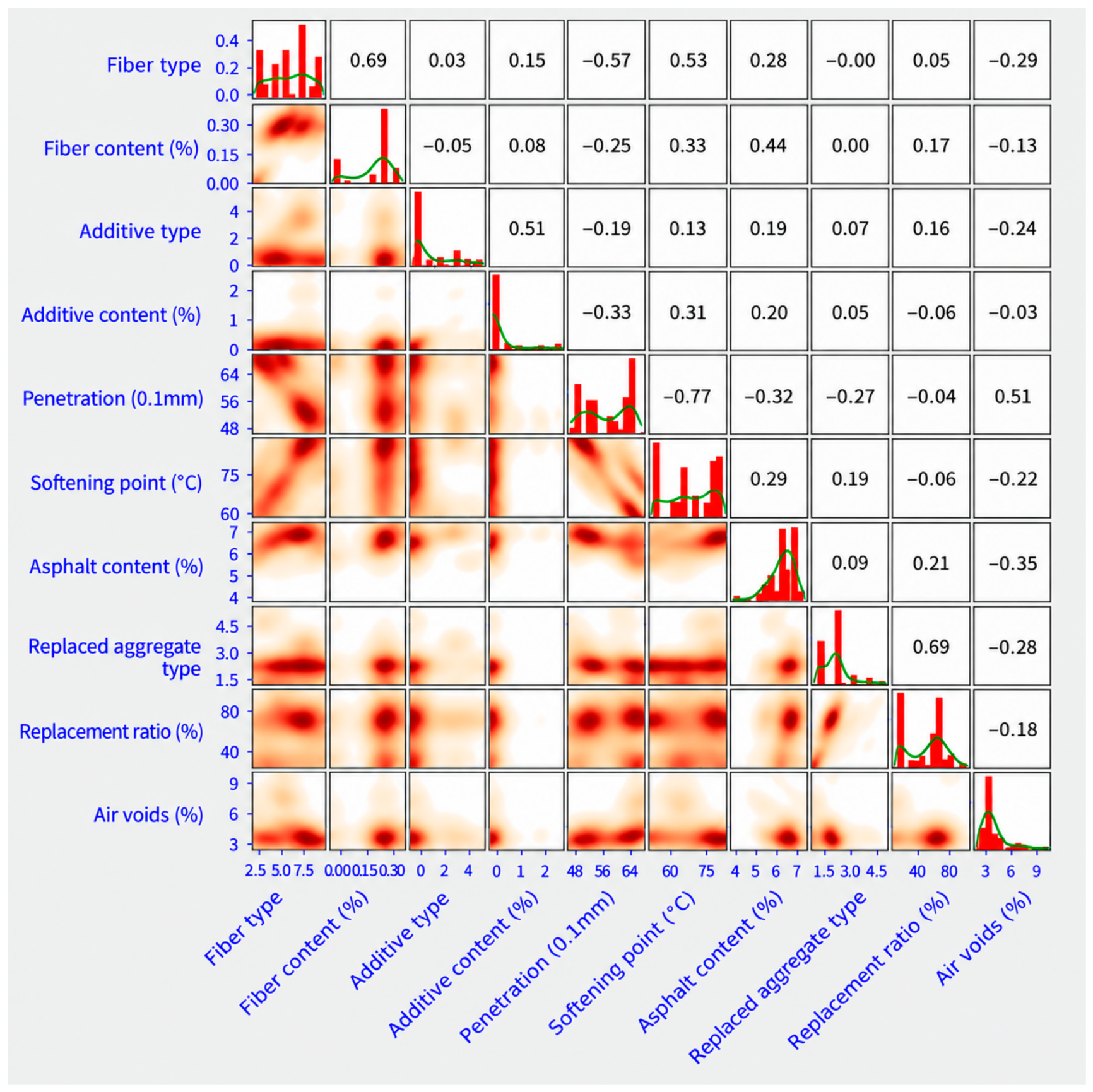
Next, the relationships among the input variables and between the input variables and the output variable were evaluated using the Pearson correlation coefficient r, with the detailed results illustrated in Figure 1. The findings indicate that most correlations among the parameters are relatively weak, except for a few strong correlations. Penetration (X5) and softening point (X6) showed a strong negative correlation (r = −0.77). Both variables were retained because they represent distinct binder properties, and their dependence was explicitly examined in Section 4.5.

Figure 1. The distribution chart and correlations between inputs and output parameters. Diagonal panels show the marginal distributions of individual variables using red histograms with green kernel density estimate (KDE) curves; lower-triangular panels show pairwise density distributions; upper-triangular panels report Pearson correlation coefficients.

After preprocessing, encoding, and conducting statistical analyses, the dataset in this study was randomly divided into two subsets. The first subset (70% of the data) was used for training the ML models and is referred to as the training dataset. The remaining 30% was used for model validation and is referred to as the testing dataset. For the detailed performance evaluation presented later in the manuscript, this 70/30 allocation is hereafter referred to as the principal train-test partition.

3. Methods

Machine learning models learn predictive relationships from observed data. In this study, XGBoost was used as the supervised prediction model, while Particle Swarm Optimization (PSO) and Grey Wolf Optimizer (GWO) were used to investigate selected XGBoost hyperparameters. The methods are described in the following subsections.

All computational analyses were performed in Python 3.13.5. XGBoost 3.1.3 was used for the XGBoost models; scikit-learn 1.8.0 was used for data partitioning, cross-validation, preprocessing, benchmark models, and permutation importance; LightGBM 4.6.0 was used for the LightGBM benchmark; and SHAP 0.50.0 was used for SHAP-based interpretation. NumPy 2.3.5, pandas 2.2.3, and Matplotlib 3.10.8 were used for numerical operations, data handling, and visualization, respectively. PSO and GWO were implemented within the Python workflow.

3.1. Extreme Gradient Boosting

XGBoost is an implementation of gradient boosting that constructs an ensemble of sequential decision trees [40]. Each new tree is fitted to reduce the residual errors of the existing ensemble [41]. Its objective combines a differentiable loss function with regularization terms that penalize model complexity. L1 and L2 regularization can reduce model complexity and susceptibility to overfitting. XGBoost also supports sparse-data handling and parallelized tree construction.

3.2. Particle Swarm Optimization

PSO is a robust, population-based stochastic optimization technique modeled on the principles of swarm intelligence [42]. The algorithm is inspired by the collective social behavior observed in natural systems, such as bird flocking or fish schooling, where individuals coordinate to find an optimal location. In the PSO framework, a set of candidate solutions, known as particles, collectively form a swarm that moves through the N-dimensional search space. Each particle maintains a memory of its own best-known position, referred to as pBest (personal best), and the swarm tracks the best position found by any particle in the entire population. At each iteration, every particle updates its velocity based on three components: (1) its current inertia, which moderates its momentum; (2) a cognitive component, which pulls it toward its pBest; and (3) a social component, which pulls it toward the gBest [43]. The particle’s position is then updated based on this new velocity. This dynamic interplay between the cognitive and social knowledge allows the swarm to effectively balance exploration and exploitation, guiding the population toward the global optimum.

3.3. Grey Wolf Optimizer

The GWO is a powerful, population-based metaheuristic algorithm inspired by the sophisticated social hierarchy and cooperative hunting behaviors of grey wolf packs. GWO mathematically models this social intelligence to guide the optimization process. The population of candidate solutions is categorized into four distinct leadership levels. The fittest solution is designated as the alpha (α), the second-best solution is the beta (β), and the third-best solution is the delta (δ). All remaining solutions are classified as omega (ω) and are considered followers. The core optimization mechanism is a simulation of the wolves’ hunt, which includes searching for, encircling, and attacking the prey. The search is uniquely guided not by a single leader, but by the collective knowledge of the three best solutions. The positions of the omega wolves are updated in the search space based on the locations of these three leaders. This strategy inherently balances the two phases of optimization: exploration (searching for prey, facilitated by parameter A > 1) and exploitation (attacking the prey, facilitated by parameter A < 1). An adaptive parameter α, which is linearly decreased from 2 to 0, controls this transition, allowing the algorithm to effectively explore the search space before converging on the optimal solution [44].

3.4. SHAP and Complementary Model-Interpretation Methods

SHapley Additive exPlanations (SHAP) were used to quantify the contribution of each input feature to individual model predictions [45]. SHAP values provide signed local attributions, and their absolute values can be aggregated across observations to obtain a global summary of model reliance on the input variables. These attributions describe the behavior of the fitted predictive model and should not be interpreted as estimates of physical causality. In addition, feature dependence can influence the allocation of attribution among correlated predictors. Accordingly, SHAP was complemented by test-set permutation feature importance, grouped permutation analysis, and feature-ablation analysis. Baseline and optimized XGBoost models were interpreted using the same input variables, and local explanations were examined for objectively selected low- and high-Va observations. This multi-method interpretation follows the distinction between model attribution and performance-based importance discussed by Molnar et al. [22].

3.5. Model Evaluation Criteria

This section defines the statistical criteria used to evaluate the agreement between the experimentally measured and model-predicted Va values. Five metrics were adopted: the coefficient of determination (R²), root mean square error (RMSE), mean absolute error (MAE), mean absolute percentage error (MAPE), and A10 index [46,47,48,49]. These metrics provide complementary information because R² describes the proportion of variation represented by the predictions, RMSE and MAE quantify absolute prediction errors, MAPE expresses relative error, and A10 measures the proportion of predictions falling within the specified agreement range.

For N observations, let y_i denote the measured Va value, ${\widehat{y}}_i$ the corresponding predicted value, and $\overline{y}$ the mean of the measured values. R² is calculated as:

$${\mathrm{R}}^2=1-{\displaystyle \frac{{\sum }_{i=1}^N(y_i-{\widehat{y}}_i{)}^2}{{\sum }_{i=1}^N(y_i-\overline{y}{)}^2}}$$

(1)

The maximum value of R² is 1, corresponding to perfect prediction. R² can also take negative values when the prediction error exceeds that obtained by using the observed mean as the predictor. Higher R² values therefore indicate better predictive agreement. RMSE is defined as:

$$\mathrm{RMSE}=\sqrt{{\displaystyle \frac{1}{N}}\sum _{i=1}^N(y_i-{\widehat{y}}_i{)}^2}$$

(2)

MAE is calculated as:

$$\mathrm{MAE}={\displaystyle \frac{1}{N}}\sum _{i=1}^N|y_i-{\widehat{y}}_i|$$

(3)

Both RMSE and MAE are expressed in the same units as Va. RMSE places greater weight on relatively large prediction errors because the residuals are squared, whereas MAE represents the average absolute magnitude of the prediction errors. Lower values of both metrics indicate better predictive performance. MAPE is calculated as:

$$\mathrm{MAPE}={\displaystyle \frac{1}{N}}\sum _{i=1}^N\left|{\displaystyle \frac{y_i-{\widehat{y}}_i}{y_i}}\right|$$

(4)

In this study, MAPE is reported as a fractional value rather than after multiplication by 100. For example, MAPE = 0.054 corresponds to a mean absolute percentage error of approximately 5.4%. Lower MAPE values indicate better predictive agreement. The A10 index is defined as:

$$\mathrm{A}10={\displaystyle \frac{1}{N}}\sum _{i=1}^{N}I\left(0.9\le {\displaystyle \frac{y_i}{{\widehat{y}}_i}}\le 1.1\right)$$

(5)

where I(⋅) is an indicator function equal to 1 when the stated condition is satisfied and 0 otherwise. A10 therefore represents the proportion of observations for which the ratio between the measured and predicted values lies between 0.9 and 1.1. Its range is 0–1, and higher values indicate better performance, with an ideal value of 1.

Accordingly, model performance is evaluated by seeking higher values of R² and A10 together with lower values of RMSE, MAE, and MAPE. Because these metrics emphasize different aspects of prediction quality, model comparisons are based on their combined interpretation rather than any single criterion.

3.6. Robustness and Sensitivity Analyses

Monte Carlo methods use repeated random sampling to characterize variability in model outcomes [50]. In predictive modeling, repeated data partitioning can be used to examine the sensitivity of estimated performance to the allocation of observations between training and testing subsets [51]. In the present study, this procedure was used as an internal split-sensitivity analysis rather than as external validation.

After completion of the hyperparameter-optimization stage, the model configuration attaining the minimum 5-fold CV RMSE among the evaluated optimization settings was carried forward without altering its selected hyperparameters. To assess sensitivity to sample allocation, this configuration was evaluated over 500 random 70/30 train-test partitions. For each partition, the model was refitted using the corresponding training observations and evaluated on the associated testing observations. The R², RMSE, MAE, MAPE, and A10 values were recorded for both subsets. Their distributions were summarized using the mean, standard deviation (SD), median, empirical 2.5th and 97.5th percentiles, and the 95% confidence interval of the mean.

A separate source-study sensitivity analysis was conducted because the 74 observations were compiled from 16 publications rather than from a single experimental program. First, the 12 observations associated with the largest contributing study listed in Table 1 were removed, and the selected model configuration was reevaluated using the remaining observations while preserving their membership in the principal train-test partition defined in Section 2. Second, a leave-one-study-out assessment was performed by withholding all observations originating from one contributing study, fitting the model using observations from the remaining studies, and predicting the withheld study. This procedure was repeated across the contributing studies, and the source-held-out predictions were pooled to evaluate transfer when observations from an entire literature source were absent from model fitting. This source-based assessment remains internal to the compiled literature database and is not treated as independent external validation.

A categorical-encoding sensitivity analysis was also conducted for the three nominal predictors X1, X3, and X8. The original integer-coded representation was compared with one-hot encoding and XGBoost native categorical handling. For one-hot encoding, each category of X1, X3, and X8 was represented by a separate binary indicator, while the remaining numerical predictors were retained unchanged. For native categorical handling, the same three variables were defined as categorical features and processed using the categorical functionality available in XGBoost. The selected model hyperparameters were held fixed across the three representations so that differences in predictive performance reflected the encoding scheme rather than a separate hyperparameter-optimization procedure. The three encodings were first evaluated using the principal train-test partition and were subsequently compared across the same 500 train-test partitions used for the split-sensitivity analysis.

3.7. Methodology of Study

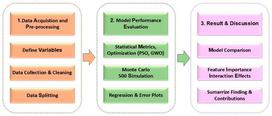
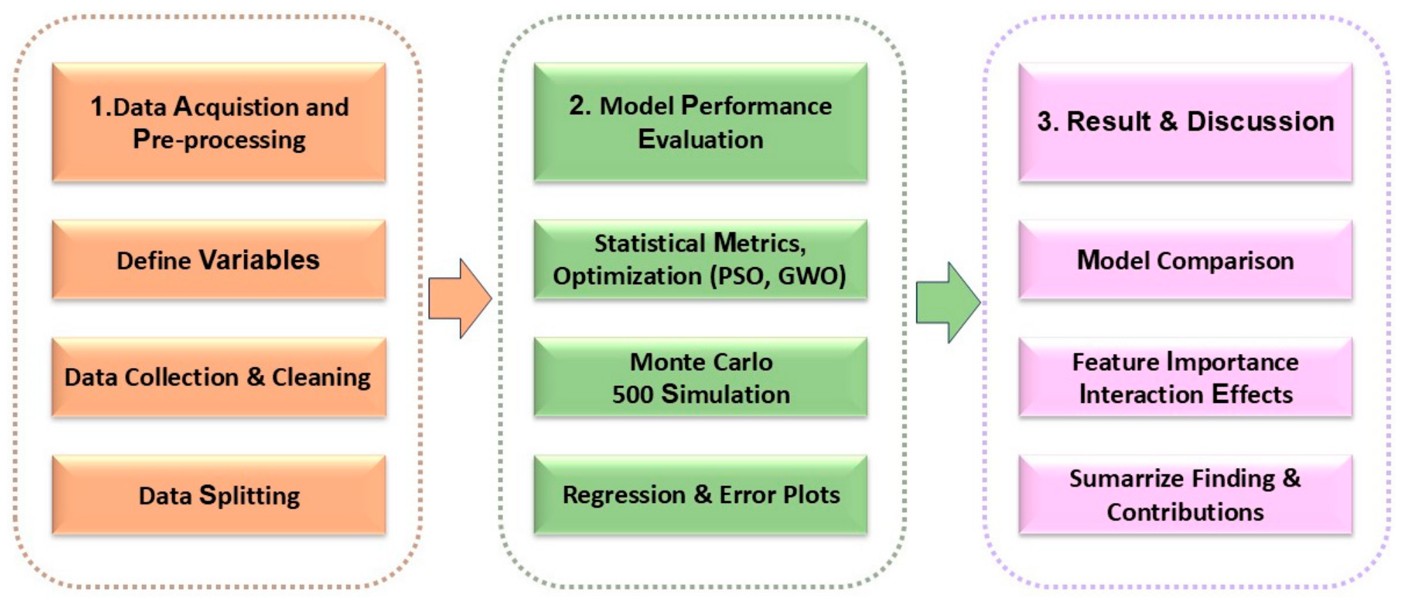
The research methodology utilized in the present study consists of three distinct phases, as depicted in the flowchart in Figure 2. The initial phase encompasses the collection and pre-processing of a dataset containing 74 experimental samples sourced from peer-reviewed literature, which is subsequently followed by the numerical encoding of categorical variables and a 70/30 partition for training and testing purposes. During the model-development stage, PSO and GWO were used to investigate the four XGBoost hyperparameters listed in Table 4. The stochastic development procedure considered 70/30 training-testing partitions, and for each candidate evaluation, the optimization objective was the mean RMSE obtained from 5-fold CV performed exclusively within the corresponding 70% training subset. Observations assigned to the corresponding 30% subset were not included in the CV folds or CV objective. After the optimization stage, Monte Carlo split-sensitivity and source-study sensitivity analyses were conducted to quantify the dependence of predictive performance on sample allocation and literature-source composition. The final phase involves a comparative analysis between the proposed approach and five standard ML benchmarks. The final phase compares the selected configuration with five benchmark models and examines model attribution using SHAP, permutation importance, grouped permutation, feature ablation, and local explanations.

Figure 2. Flowchart of the research methodology.

Table 4. The search domains of hyperparameters in this study.

No.	Hyperparameter	The Search Domain	Description
1	n_estimators	10–300	Total number of boosting iterations
2	learning_rate	0.01–0.3	Step-size shrinkage used to control the contribution of each boosting iteration
3	max_depth	3–8	Maximum depth of each regression tree
4	subsample	0.2–0.9	Fraction of samples used per tree

Given the modest dataset size (N = 74), model complexity was constrained during development rather than allowing unrestricted growth of the ensemble. The metaheuristic search was limited to the four XGBoost hyperparameters listed in Table 4, with bounded domains of 10–300 estimators, learning rate of 0.01–0.30, maximum tree depth of 3–8, and subsampling of 0.2–0.9. The fitted model also retained tree-complexity and regularization controls through min_child_weight, gamma, and L1 regularization. Five-fold CV was incorporated into the development-stage objective so that candidate configurations were evaluated across multiple training subsets rather than only by fitting error. These controls reduce model flexibility and provide a structured model-selection procedure, but they do not eliminate the uncertainty arising from the small and heterogeneous database. For this reason, the final model is additionally evaluated using repeated random partitions, source-study sensitivity, categorical-encoding sensitivity, and comparison with alternative ML models.

A strong correlation was observed between penetration (X5) and softening point (X6), with r = −0.77, but both variables were retained because they represent distinct binder properties included in the defined predictor space. Because predictor dependence can affect the distribution of feature importance and attribution, the individual and joint contributions of X5 and X6 were examined using SHAP, permutation importance, grouped permutation, and feature-ablation analyses, as discussed in Section 4.5.

For the comparative evaluation, the five benchmark algorithms were subjected to a systematic hyperparameter search using the same training subset and the same 5-fold CV structure. RMSE was used as the model-selection criterion, and 50 candidate hyperparameter configurations were evaluated for each benchmark algorithm. The configuration with the lowest mean CV RMSE was subsequently refitted using the complete principal training subset and evaluated on the common testing subset. This procedure was used to avoid comparing the proposed XGB_GWO_40 configuration only against untuned or default benchmark implementations. Because the GWO/PSO development of the proposed model and the benchmark searches do not represent identical computational budgets, the comparison therefore concerns the evaluated model configurations and does not establish intrinsic superiority of one algorithm over another.

4. Results and Discussion

4.1. Hyperparameter Investigation

The predictive performance of the XGBoost model is fundamentally dependent on the precise calibration of its key hyperparameters. Search domains for the four primary hyperparameters selected for tuning, n_estimators, learning_rate, max_depth, and subsample, are detailed in Table 4. These are the hyperparameters that greatly influence the predictive performance of the model [52,53]. This section compares the PSO and GWO optimization settings and identifies the XGBoost configuration carried forward to the subsequent analyses. The optimization objective was the mean 5-fold CV RMSE calculated within the training portion of the development-stage data partitions described in Section 3.7. Consequently, the values reported in Table 5 represent development-stage CV objectives rather than CV results obtained from the principal 70/30 partition used later for detailed prediction.

Table 5. Development-stage optimization performance of the PSO and GWO configurations.

Metaheuristic	Pop Size	Minimum Development-Stage 5-Fold CV RMSE (%)	Mean Time (s)
PSO	10	0.422	2.99
	20	0.441	4.11
	30	0.393	5.69
	40	0.389	9.31
GWO	10	0.416	3.11
	20	0.424	4.67
	30	0.407	8.99
	40	0.371	8.75

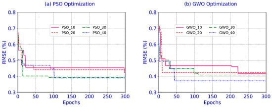
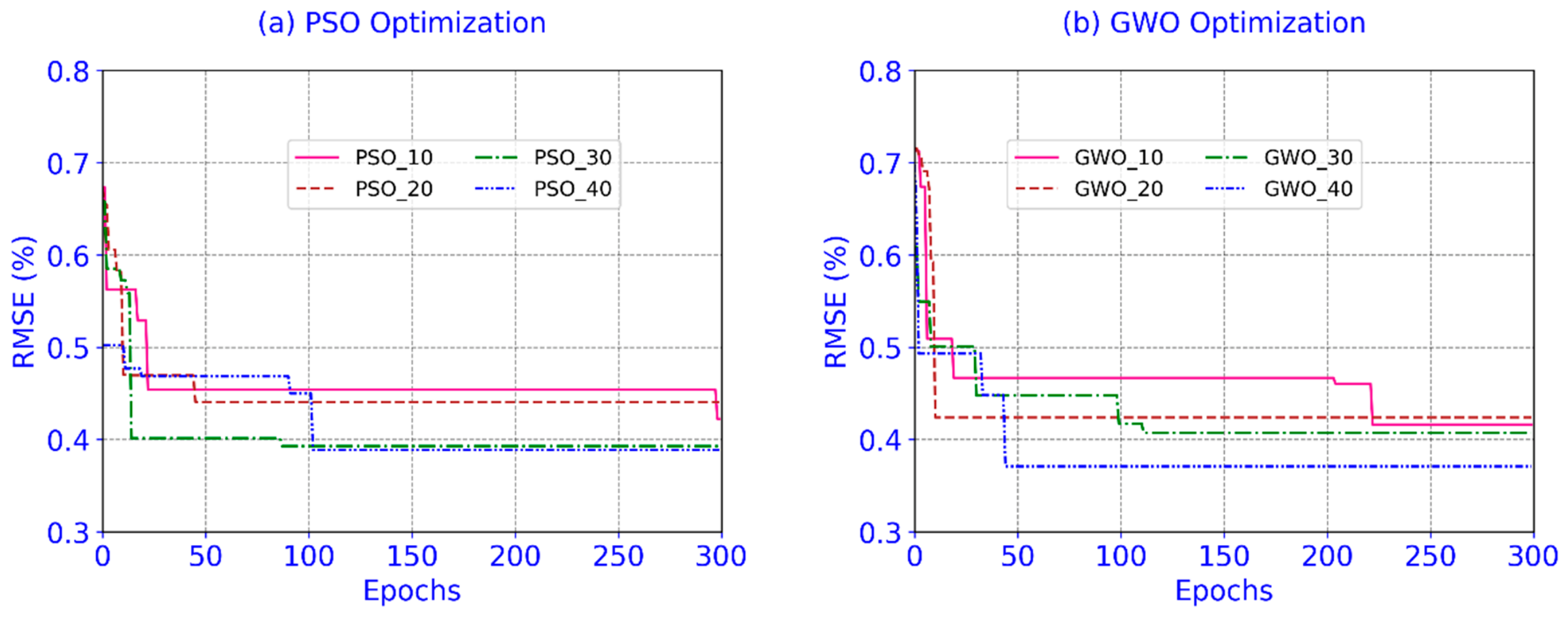
To identify the best-performing configuration under the development-stage objective, the optimization process aimed to minimize the RMSE evaluated through 5-fold CV. Both the PSO and GWO algorithms were executed with four distinct population sizes: 10, 20, 30, and 40 over 300 optimization epochs. Optimization convergence curves for all eight configurations are presented in Figure 3, while Table 5 summarizes their minimum development-stage CV RMSE and mean computation time. GWO with a population size of 40 produced the lowest CV RMSE of 0.371%, compared with 0.389% for PSO with a population size of 40. The corresponding GWO solution yielded n_estimators = 226, learning_rate = 0.3, max_depth = 6, and subsample = 0.9. This configuration, hereafter denoted XGB_GWO_40, was selected for the subsequent robustness, comparative, prediction, and interpretability analyses.

Figure 3. Convergence of the development-stage 5-fold CV RMSE during 300 epochs of PSO and GWO optimization.

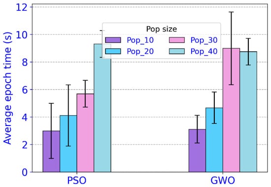
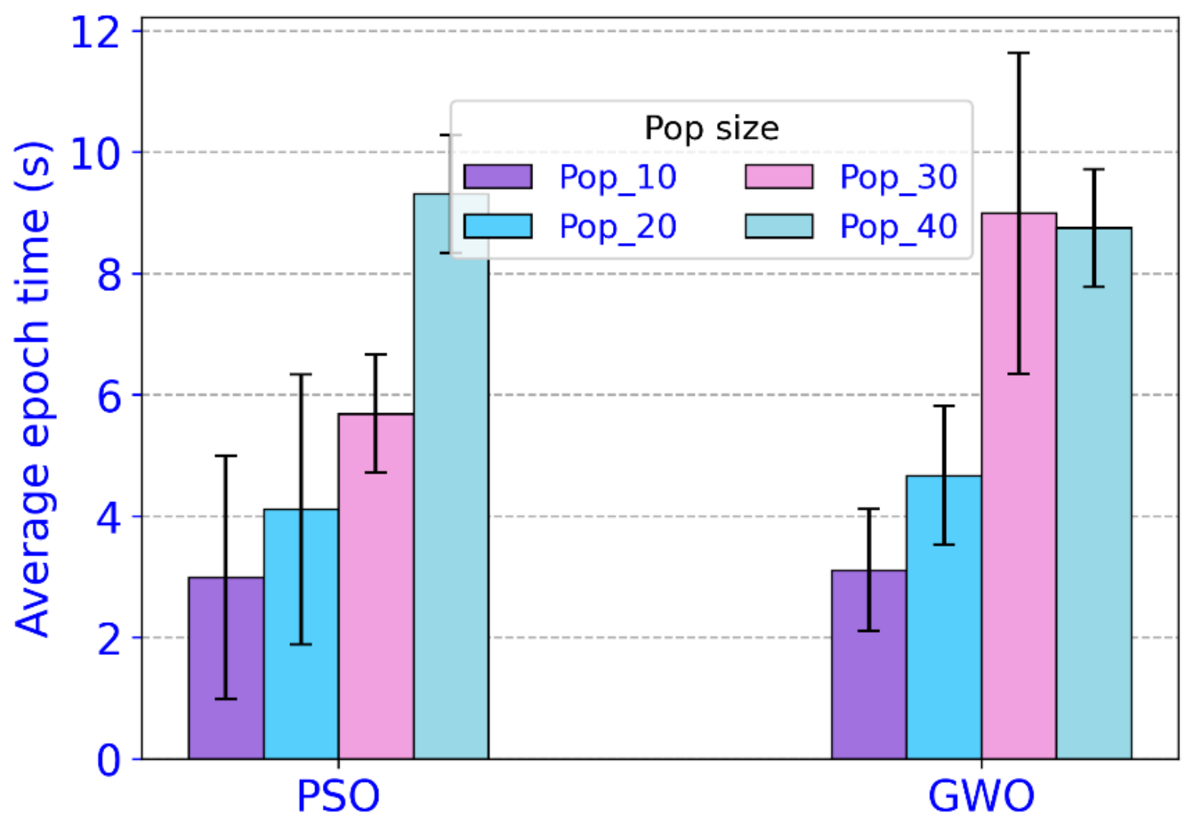
In addition to the optimization objective, computational time was examined for the different population sizes, as shown in Figure 4. The bars represent the average epoch computation time, while the error bars show the corresponding variability across the recorded epochs. For PSO, the average epoch time increases from 2.99 s at a population size of 10 to 9.31 s at a population size of 40. A similar increase is generally observed for GWO, from 3.11 s at population 10 to 8.75 s at population 40, although GWO with population 30 exhibits a slightly higher average time of 8.99 s. Thus, increasing population size generally increases computational demand because more candidate solutions are evaluated during each optimization epoch. The selection of GWO with population 40 is nevertheless based on its lower CV RMSE rather than computational time alone.

Figure 4. Average computation time per optimization epoch for PSO and GWO at population sizes of 10, 20, 30, and 40.

4.2. Robustness and Sensitivity Analyses

Following the optimization comparison in Section 4.1, the selected XGB_GWO_40 configuration was examined using three complementary sensitivity analyses. The first quantified variation in predictive performance across alternative 70/30 allocations of individual observations. The second examined sensitivity to literature-source composition through largest-source removal and leave-one-study-out evaluation. The third assessed the effect of categorical representation by comparing integer coding, one-hot encoding, and XGBoost native categorical handling. Together, these analyses assess sensitivity to sample allocation, source composition, and categorical encoding; none constitutes independent external validation.

4.2.1. Monte Carlo Split-Sensitivity Analysis

The XGB_GWO_40 hyperparameter configuration was held fixed and evaluated over 500 random 70/30 train-test partitions. For each partition, the model was refitted on the training subset and evaluated using the corresponding testing subset. Table 6 summarizes the resulting distributions of R², RMSE, MAE, MAPE, and A10 for the training and testing datasets.

Table 6. Statistical summary of model performance over 500 random 70/30 train-test partitions.

Dataset	Metric	Mean	SD	Median	2.5–97.5th Percentile	95% CI of Mean
Training	R2	0.968	0.009	0.970	0.948–0.981	0.967–0.969
	RMSE (%)	0.255	0.024	0.256	0.207–0.302	0.253–0.257
	MAE (%)	0.172	0.014	0.173	0.145–0.200	0.171–0.174
	MAPE	0.0358	0.0027	0.0356	0.0310–0.0414	0.0355–0.0360
	A10	0.947	0.024	0.941	0.902–0.980	0.945–0.949
Testing	R2	0.379	0.629	0.519	−0.815–0.850	0.320–0.429
	RMSE (%)	0.977	0.254	0.971	0.514–1.455	0.954–0.999
	MAE (%)	0.597	0.142	0.595	0.357–0.905	0.584–0.609
	MAPE	0.1186	0.0262	0.1170	0.0752–0.1823	0.1163–0.1209
	A10	0.620	0.090	0.609	0.435–0.783	0.612–0.627

SD = standard deviation; CI = confidence interval of the mean. The percentile interval describes the empirical distribution of performance across partitions and should not be an external-validation interval.

The training results were comparatively stable across partitions. The mean training R² was 0.968, with an SD of 0.009, while the mean RMSE was 0.255%, with an SD of 0.024%. The corresponding empirical 2.5–97.5th percentile intervals were 0.948–0.981 for R² and 0.207–0.302% for RMSE. This narrow dispersion indicates that the fitted model consistently reproduced the training observations under alternative data allocations.

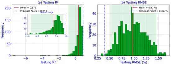
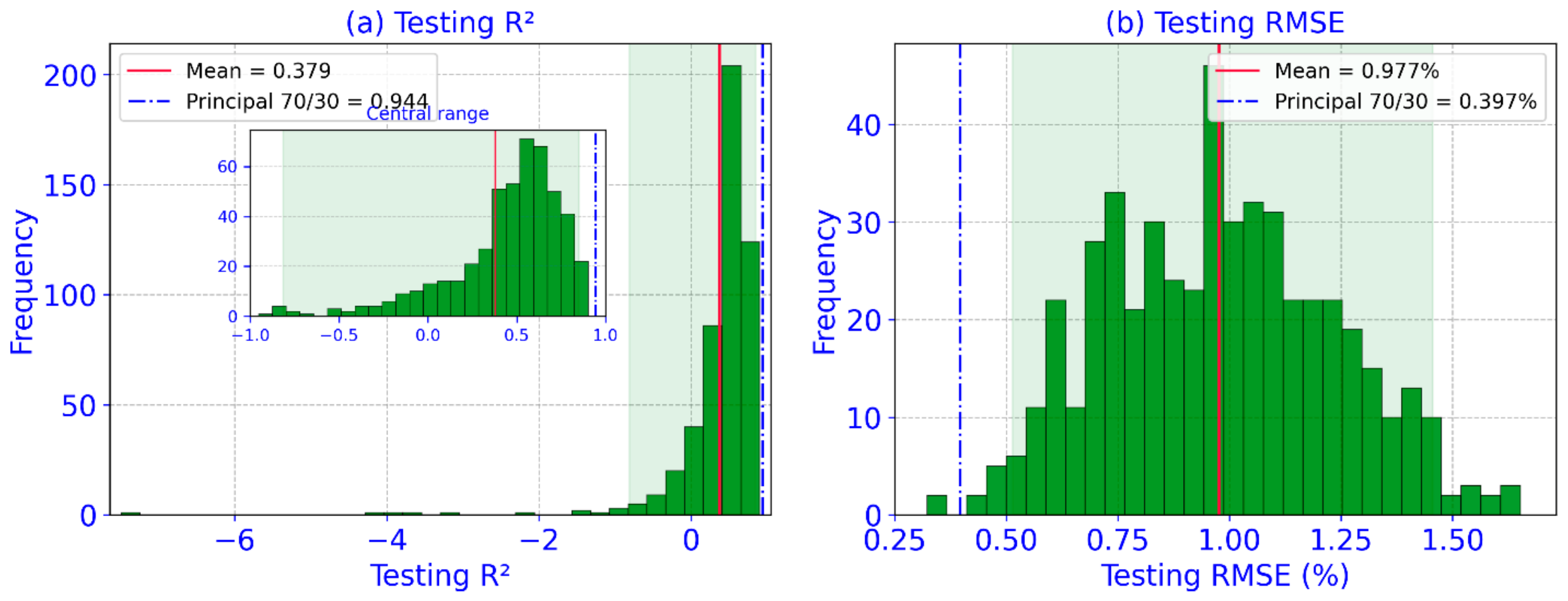
The testing results showed substantially greater sensitivity to the composition of the 30% testing subset. Across the 500 partitions, the mean testing R² was 0.379, with an SD of 0.629 and a median of 0.519. The empirical 2.5–97.5th percentile interval extended from −0.815 to 0.850. Testing RMSE had a mean of 0.977%, an SD of 0.254%, and an empirical interval of 0.514–1.455%. MAE, MAPE, and A10 showed the same broader between-partition variability relative to the training results. The pronounced variability of testing R² is particularly relevant for the present small testing subsets because R² depends on the variance of the observed Va values contained in each partition; consequently, different compositions of the 23-observation testing subset can produce substantial variation in this metric.

Figure 5 presents the actual testing R² and RMSE distributions. The principal 70/30 evaluation reported subsequently in Section 4.3 yielded R² = 0.944 and RMSE = 0.397%. These values are shown in Figure 5 as separate reference lines rather than as observations from the 500-partition ensemble. They lie toward the favorable end of the repeated-partition performance distribution. Accordingly, the R² = 0.944 value is retained as the result of the principal train-test evaluation, but it is not the expected performance under arbitrary repartitioning of the 74 observations. The repeated-partition analysis therefore provides a quantitative measure of internal sensitivity to sample allocation. It does not establish performance on data generated outside the compiled literature database, and it is not used as evidence of external validity.

Figure 5. Monte Carlo assessment of sensitivity to train-test allocation over 500 random 70/30 partitions for the selected XGB_GWO_40 model: (a) distribution of testing R²; and (b) distribution of testing RMSE. Green bars show the frequency distributions obtained from the 500 partitions, while the light-green shaded region indicates the central range of the corresponding testing-performance distribution. The red solid line denotes the mean value, and the blue dash-dot line denotes the result from the principal 70/30 partition.

4.2.2. Source-Study Sensitivity Analysis

Random train-test repartitioning evaluates sensitivity to individual-observation allocation, but observations originating from the same publication can still occur in both subsets. Because the database combines 74 observations from 16 literature sources, an additional source-study analysis was conducted to examine whether the reported performance depended strongly on particular contributing studies.

The first assessment removed the 12 observations contributed by the largest source in Table 1. Among the remaining 62 observations, 43 retained their original training membership, and 19 retained their original testing membership from the principal partition. The resulting testing performance was R² = 0.819, RMSE = 0.222%, MAE = 0.178%, MAPE = 0.045, and A10 = 0.895, as summarized in Table 7. Although R² decreased relative to the principal result of 0.944, the absolute-error metrics did not deteriorate; RMSE and MAE were lower after removal of the largest source. This combination indicates that the reduction in R² is influenced by the changed distribution and variance of Va in the reduced dataset rather than by a corresponding increase in absolute prediction error. The result also indicates that the favorable predictive behavior observed in the principal partition is not attributable solely to the largest contributing source.

Table 7. Sensitivity of predictive performance to literature-source composition.

Evaluation Scheme	Testing/Evaluation Data	R2	RMSE (%)	MAE (%)	MAPE	A10
Principal 70/30 evaluation	23 testing observations	0.944	0.397	0.262	0.054	0.826
Largest contributing source removed	19 testing observations from 62 retained observations	0.819	0.222	0.178	0.045	0.895
Leave-one-study-out, pooled predictions	74 pooled source-held-out predictions	−0.339	1.694	1.166	0.230	0.297

The leave-one-study-out analysis evaluates transfer between literature sources contained within the compiled database; it does not constitute independent external validation.

A more stringent assessment was obtained by withholding one complete literature source at a time. When the source-held-out predictions were pooled across the database, the resulting R² was −0.339, with RMSE = 1.694%, MAE = 1.166%, MAPE = 0.230, and A10 = 0.297. The substantial deterioration relative to the row-level principal evaluation demonstrates that prediction for a completely unrepresented source-study domain is considerably more difficult than prediction among observations belonging to the material domain already represented during model fitting.

These source-study results define an important boundary on the interpretation of the model. The principal testing result of R² = 0.944 demonstrates high predictive accuracy for the selected within-database partition, whereas the leave-one-study-out result does not support a claim of unrestricted transfer to previously unseen experimental domains. Independent laboratory or field datasets representing the intended deployment conditions are therefore required before external generalization can be established.

4.2.3. Categorical-Encoding Sensitivity

This subsection examines whether the predictive results depend strongly on the numerical representation assigned to the three nominal variables X1, X3, and X8. The original integer coding was compared with one-hot encoding and XGBoost native categorical handling using the same selected model configuration. The comparison was performed first on the principal train-test partition and then across the 500 partitions used in Section 4.2.1.

The principal-partition results are summarized in Table 8. Integer coding produced the highest R² of 0.944 and the lowest RMSE, MAE, and MAPE, with values of 0.397%, 0.262%, and 0.054, respectively. One-hot encoding produced R² = 0.928, RMSE = 0.449%, MAE = 0.294%, and MAPE = 0.057, while XGBoost native categorical handling yielded R² = 0.892, RMSE = 0.551%, MAE = 0.319%, and MAPE = 0.066. A10 was 0.826 for both integer coding and native categorical handling and 0.783 for one-hot encoding. Although the numerical metrics differ, the predictions produced by the alternative representations remain strongly related to those of the integer-coded model. The correlation between integer-coded and one-hot predictions is r = 0.981, while that between integer-coded and native-categorical predictions is r = 0.973. Thus, changing the categorical representation modifies individual predictions and aggregate error levels but does not produce a fundamentally different prediction pattern on the principal partition.

Table 8. Sensitivity of XGB_GWO_40 predictive performance to categorical encoding.

Encoding	R2	RMSE (%)	MAE (%)	MAPE	A10
Principal 70/30 evaluation
Integer coding	0.944	0.397	0.262	0.054	0.826
One-hot encoding	0.928	0.449	0.294	0.057	0.783
Native categorical	0.892	0.551	0.319	0.066	0.826
Testing performance across 500 train-test partitions, mean ± SD
Integer coding	0.379 ± 0.629	0.977 ± 0.254	0.597 ± 0.142	0.119 ± 0.026	0.620 ± 0.090
One-hot encoding	0.412 ± 0.554	0.953 ± 0.270	0.561 ± 0.147	0.109 ± 0.025	0.656 ± 0.093
Native categorical	0.385 ± 0.594	0.970 ± 0.265	0.572 ± 0.144	0.112 ± 0.026	0.650 ± 0.091

The broader 500-partition comparison provides a complementary result, as shown in Table 8. One-hot encoding yields the highest mean testing R² of 0.412, compared with 0.379 for integer coding and 0.385 for native categorical handling. Its mean RMSE is also slightly lower at 0.953%, compared with 0.977% and 0.970%, respectively. Similar modest improvements are observed for MAE, MAPE, and A10. Therefore, the principal-partition advantage of integer coding is not reproduced consistently across alternative data allocations; on average, one-hot encoding performs slightly better.

The encoding sensitivity analysis therefore provides two complementary findings. First, the strong principal-partition performance is not created solely by the artificial numerical ordering of X1, X3, and X8, because both alternative categorical representations retain comparatively high predictive performance and produce strongly correlated predictions. Second, categorical representation is not completely inconsequential: one-hot encoding provides modestly better average performance across repeated partitions. Accordingly, the integer-coded representation is retained as the primary model for continuity with the original nine-variable framework, but its categorical codes are interpreted only as nominal identifiers, and the sensitivity to alternative encodings is explicitly acknowledged when assessing model stability.

4.3. Representative Prediction Results

This section evaluates XGB_GWO_40 on the principal 70/30 partition defined in Section 2. This evaluation is distinct from the development-stage CV objective reported in Table 5. The comprehensive statistical performance of the model on the training, testing, and full datasets is summarized in Table 9. The model demonstrates exceptional predictive power, achieving R² values of 0.956 for the training set and 0.944 for the testing set. The calculated R² values establish a strong predictive agreement between the generated predictions and the corresponding experimental data. This predictive capability is further corroborated by the quantified error metrics, yielding RMSE values of 0.286 for the training set and 0.397 for the testing set, accompanied by MAE measurements of 0.187 and 0.262 for the respective data partitions. These results indicate good predictive agreement for this particular allocation. However, Section 4.2 shows that performance varies across alternative sample allocations and source compositions; the principal-partition result therefore does not establish unrestricted external generalization.

Table 9. Values of statistical criteria of the best model for Va.

Metrics	R2	RMSE (%)	MAE (%)	MAPE	A10
Training set	0.956	0.286	0.187	0.038	0.961
Testing set	0.944	0.397	0.262	0.054	0.826
Full dataset	0.951	0.324	0.210	0.043	0.919

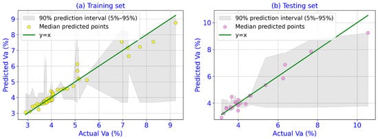
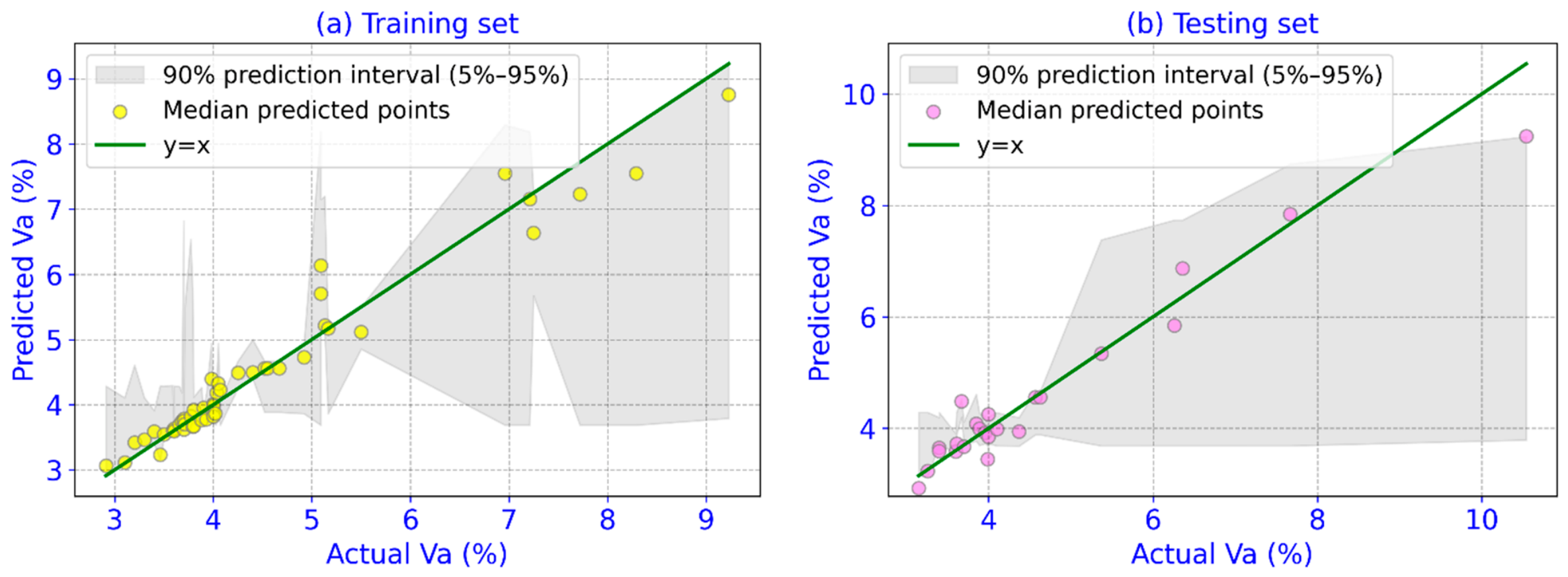
A visual confirmation of this high accuracy is provided in Figure 6, which displays the regression plots for both the training and testing sets. These plots compare the predicted Va values with the corresponding experimental values. In both plots, the data points cluster around the y = x line. The clustering of the data points around the y = x line is consistent with the R² values and error metrics reported in Table 9.

Figure 6. The regression graphs for the values of outputs between simulation and experiment.

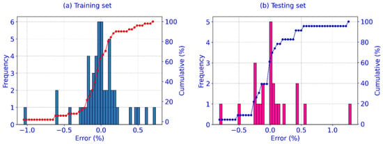
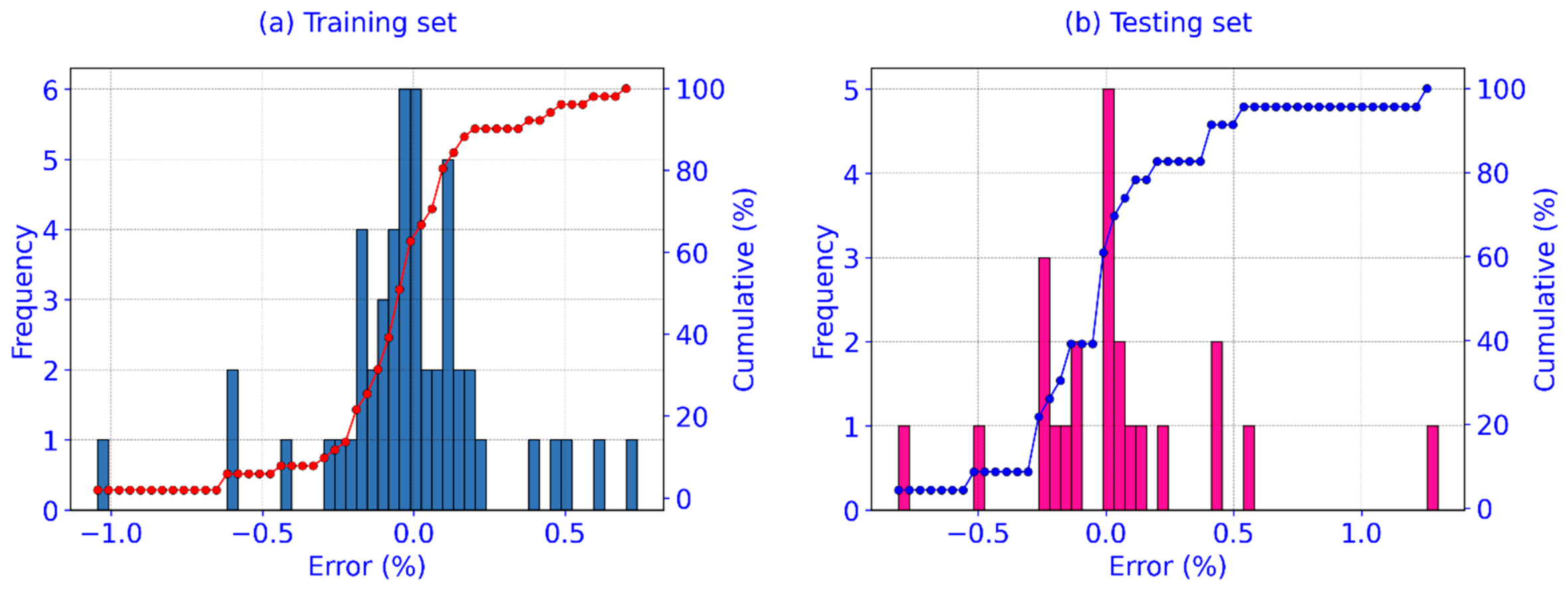
To further assess the model’s precision and potential bias, the distribution of prediction errors was analyzed, as shown in Figure 7. The histograms for both the training (Figure 7a) and testing (Figure 7b) sets reveal that the prediction errors are predominantly concentrated around zero. The cumulative frequency curves in both plots rise sharply near the zero-error mark, indicating that most predictions have very small errors. The concentration of prediction errors around zero indicates that no obvious systematic offset is apparent for the principal training and testing partitions.

Figure 7. Histograms and cumulative distributions of prediction errors for the (a) Training set and (b) Testing set.

Collectively, the statistical metrics, regression plots, and error distributions demonstrate high predictive accuracy for the principal 70/30 evaluation. The broader stability and transferability of the model should, however, be considered together with the partition- and source-study sensitivity results reported in Section 4.2.

4.4. Model Comparison

This section compares the predictive behavior of the proposed XGB_GWO_40 configuration with five alternative tree-based ML models after systematic tuning of the benchmark models. The comparison uses the same principal training and testing observations for all models so that differences in the reported metrics reflect the fitted model configurations rather than different data allocations. The updated training and testing results are summarized in Table 10 and visualized in Figure 8.

Table 10. Model evaluation results for the Va dataset.

Dataset	Metric	XGB_GWO_40	HistGB	LightGBM	GradientBoost	Decision Tree	Random Forest
Train	R2	0.956	0.625	0.674	0.637	0.767	0.692
	RMSE (%)	0.286	0.830	0.774	0.816	0.654	0.752
	MAE (%)	0.187	0.538	0.501	0.548	0.376	0.471
	MAPE	0.038	0.111	0.100	0.114	0.074	0.094
	A10	0.961	0.627	0.608	0.529	0.706	0.647
Test	R2	0.944	0.633	0.673	0.732	0.768	0.712
	RMSE (%)	0.397	1.014	0.957	0.867	0.806	0.898
	MAE (%)	0.262	0.534	0.479	0.464	0.447	0.399
	MAPE	0.054	0.103	0.087	0.084	0.081	0.068
	A10	0.826	0.652	0.696	0.609	0.696	0.870

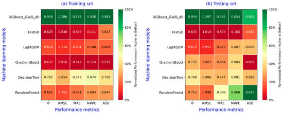
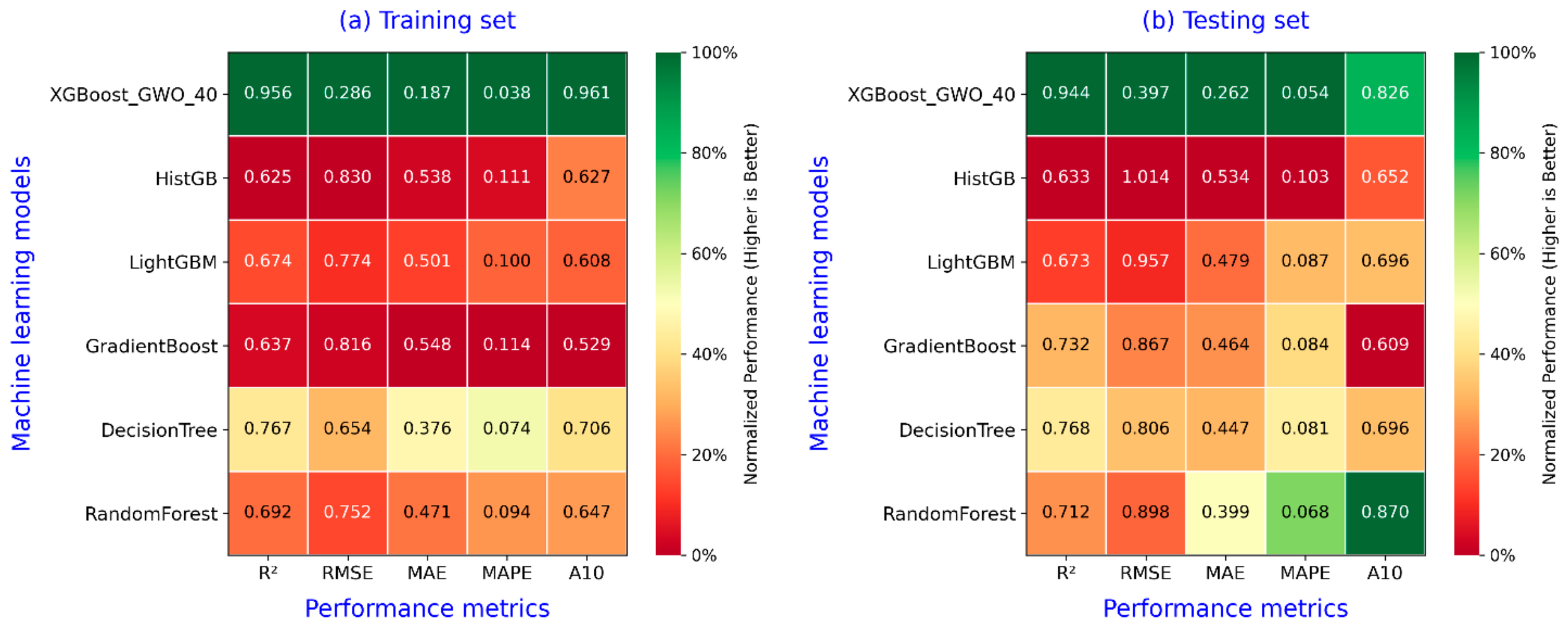
Figure 8. Comparative performance of XGB_GWO_40 and the systematically tuned benchmark models for: (a) the principal training subset and (b) the principal testing subset.

On the training subset, XGB_GWO_40 achieves R² = 0.956, RMSE = 0.286%, MAE = 0.187%, MAPE = 0.038, and A10 = 0.961. The tuned benchmark models produce lower training R² values ranging from 0.625 for HistGB to 0.767 for Decision Tree. Unlike the original Decision Tree result, which approached a nearly perfect training fit, the tuned tree configuration has a substantially smaller train-test gap, indicating that the CV-based tuning procedure selected a less complex configuration. The same pattern is evident for Random Forest and GradientBoost, whose training errors are higher than those of XGB_GWO_40 but remain closer to their corresponding testing errors.

The testing results provide a more relevant comparison of the evaluated configurations. XGB_GWO_40 achieves the highest testing R² of 0.944 and the lowest RMSE, MAE, and MAPE, with values of 0.397%, 0.262%, and 0.054, respectively. Decision Tree produces the second-highest R² at 0.768 and an RMSE of 0.806%, followed by GradientBoost with R² = 0.732 and RMSE = 0.867%. Random Forest yields R² = 0.712 and RMSE = 0.898%, but it produces the highest A10 value of 0.870 compared with 0.826 for XGB_GWO_40. Thus, the metric ranking is not identical for every performance criterion, even though XGB_GWO_40 provides the strongest combination of R² and absolute error measures on the principal testing partition.

Systematic tuning produced testing R² values of 0.633 and 0.673 for HistGB and LightGBM, respectively. These results describe the tuned HistGB and LightGBM configurations and do not support attributing their performance to an inherent limitation of histogram-based tree construction. Accordingly, the benchmark comparison is restricted to the empirical predictive performance obtained under the stated tuning procedures.

As an additional tuning-budget diagnostic, an ordinary XGBoost model was subjected to the same 50-candidate CV search used for the benchmark models. The selected configuration obtained a testing R² of approximately 0.717 and RMSE of 0.890%, compared with R² = 0.944 and RMSE = 0.397% for XGB_GWO_40. This result indicates that the strong principal-partition performance is not reproduced simply by applying XGBoost under the same 50-candidate benchmark search. At the same time, because the GWO procedure represents a more extensive model-development effort, this comparison is not interpreted as proof that GWO or XGBoost is universally superior to the alternative algorithms.

Overall, Table 10 supports XGB_GWO_40 as the strongest evaluated configuration on the principal partition for R², RMSE, MAE, and MAPE, while Random Forest performs better according to A10. These results support the selection of XGB_GWO_40 for the detailed interpretation performed in Section 4.5, but the broader partition- and source-study analyses in Section 4.2 remain necessary when considering the stability and transferability of the model beyond this principal evaluation.

4.5. Model Interpretation and Attribution Stability

This section compares model interpretation at both global and local levels for the baseline XGBoost model and XGB_GWO_40. Global feature attribution is quantified using SHAP and compared with performance-based importance obtained from test-set permutation feature importance (PFI), grouped permutation of correlated variables, and feature ablation. Feature-effect patterns are examined using SHAP dependence results for both models, while local attributions are compared for the same objectively selected low- and high-Va testing observations. These complementary analyses distinguish model-specific attribution from predictive importance and avoid relying on a single interpretation measure.

The predictive performances of the baseline and optimized XGBoost models were first compared using the same principal training-testing partition. The baseline XGBoost model achieved an R² of 0.914, RMSE of 0.491%, MAE of 0.354%, and MAPE of 0.071 on the testing subset. After optimization, XGB_GWO_40 achieved an R² of 0.944, RMSE of 0.397%, MAE of 0.262%, and MAPE of 0.054. Therefore, the optimized configuration provides lower prediction errors and a higher R² on the principal testing partition. The interpretability comparison was subsequently performed to determine whether this improvement in predictive performance was accompanied by a substantial change in the variables used by the model.

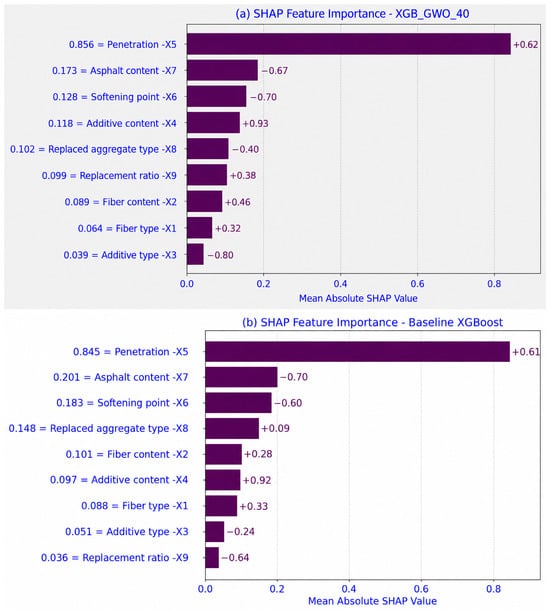
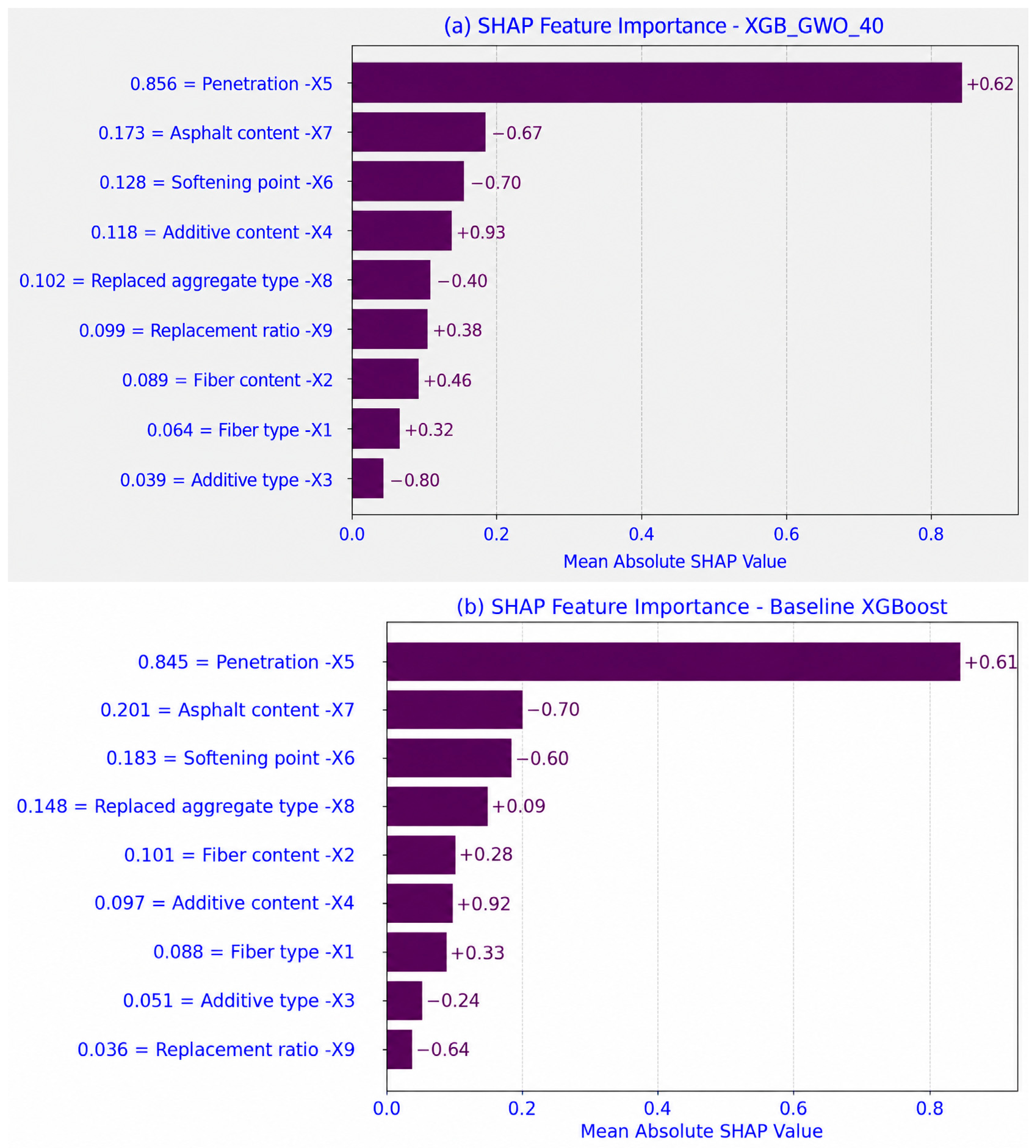
The global SHAP feature importance for XGB_GWO_40 is presented in Figure 9a, while the corresponding baseline XGBoost result is shown in Figure 9b. The global importance was calculated from the mean absolute SHAP value of each variable across the complete dataset. For XGB_GWO_40, penetration (X5) has the highest mean absolute SHAP value of 0.856, followed by asphalt content (X7) at 0.173, softening point (X6) at 0.128, and additive content (X4) at 0.118. The remaining variables, including the aggregate-replacement parameters (X8 and X9) and fiber-related variables (X1 and X2), have lower average SHAP magnitudes. The prominence of binder-related variables in the fitted model is consistent with previous asphalt-material studies, showing that binder properties, binder content, and compaction conditions are closely associated with mixture volumetric behavior [54,55,56].

Figure 9. Global SHAP feature importance for (a) XGB_GWO_40 and (b) baseline XGBoost, ranked by mean absolute SHAP value.

A similar attribution structure is observed for the baseline XGBoost model. Penetration (X5) remains the highest-ranked variable, with a mean absolute SHAP value of 0.845, followed by asphalt content (X7) at 0.201 and softening point (X6) at 0.183. The complete SHAP rankings of the baseline and optimized models have a rank correlation of approximately 0.83. Therefore, optimization does not produce a fundamentally different ordering of the principal variables. Instead, the main changes occur among the lower-ranked predictors, whereas X5, X7, and X6 remain the three leading variables in both models. This result indicates that the improved performance of XGB_GWO_40 is obtained while largely preserving the principal attribution structure already present in the baseline XGBoost model.

Because SHAP describes feature attribution within the fitted model, the global ranking was also examined using test-set PFI. For each input variable, the observed feature values were repeatedly permuted while all other variables and the fitted model were retained, and the resulting increase in RMSE was used as a measure of predictive importance. For XGB_GWO_40, permutation of X5 produced the largest deterioration, increasing the test RMSE by approximately 1.578 percentage points (Table 11). The next largest increases were observed for X7 (0.269), X9 (0.225), and X8 (0.117). The same general result was obtained for the baseline XGBoost model, for which X5 permutation increased RMSE by approximately 1.580 percentage points. In that model, X8 and X7 produced the next largest increases of approximately 0.471 and 0.432 percentage points, respectively. Thus, the two interpretation methods agree strongly regarding X5, while the different rankings of some secondary variables show that feature importance depends partly on the question addressed by the interpretation method.

Table 11. Global interpretation comparison between baseline XGBoost and XGB_GWO_40.

Feature	XGB_GWO_40 Mean |SHAP|	Baseline Mean |SHAP|	XGB_GWO_40 PFI ΔRMSE (%)	Baseline PFI ΔRMSE (%)
X5—Penetration	0.856	0.845	1.578	1.580
X7—Asphalt content	0.173	0.201	0.269	0.432
X6—Softening point	0.128	0.183	0.066	0.090
X4—Additive content	0.118	0.097	0.019	0.002
X8—Replaced aggregate type	0.102	0.148	0.117	0.471
X9—Replacement ratio	0.099	0.036	0.225	0.013
X2—Fiber content	0.089	0.101	0.066	0.099
X1—Fiber type	0.064	0.088	0.038	0.019
X3—Additive type	0.039	0.051	0.005	−0.009

Particular attention was given to penetration (X5) and softening point (X6) because the initial correlation analysis showed a strong negative correlation between these variables (r = −0.77). This dependence can affect the attribution assigned to correlated features and therefore requires additional verification. For XGB_GWO_40, permutation of X5 alone increased RMSE by approximately 1.594 percentage points, whereas permutation of X6 alone increased RMSE by only 0.059 percentage points. When X5 and X6 were permuted jointly, RMSE increased by approximately 1.593 percentage points. These results indicate that most of the predictive information represented by this correlated pair is associated with X5 in the fitted optimized model; however, they do not establish that X5 represents an independent causal effect.

Feature ablation provided a complementary assessment by retraining the optimized model after removing individual variables. Removing X5 reduced the testing R² from 0.944 to 0.843 and increased RMSE from 0.397% to 0.663%. Removing X6 alone did not deteriorate the principal-partition performance, producing an R² of 0.948 and RMSE of 0.383%, whereas jointly removing X5 and X6 reduced R² to 0.747 and increased RMSE to 0.843%. The analysis also showed that X7 remains an important predictor because removing asphalt content reduced R² to 0.807 and increased RMSE to 0.735%. X5 is therefore an important and consistently identified predictor, but it is not the sole determinant of the model output. The ablation results also demonstrate why attribution magnitude should be interpreted together with complementary predictive-sensitivity analyses when correlated or interacting variables are present.

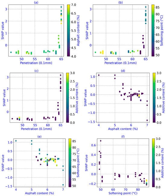
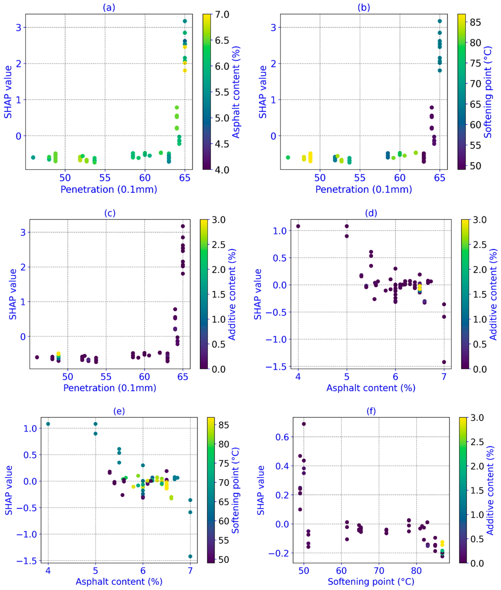
Beyond the global feature ranking, the SHAP dependence plots in Figure 10 were examined to determine how the contribution of the leading variables changes over the ranges represented in the database. Figure 10a–c shows the behavior of penetration (X5) in combination with asphalt content (X7), softening point (X6), and additive content (X4). The relationship is clearly non-linear. Strong positive SHAP contributions occur primarily toward the upper end of the penetration range, particularly around 65 (0.1 mm). However, observations between approximately 60 and 63 (0.1 mm) still contain predominantly negative SHAP contributions, and the transition is not sufficiently consistent to support an exact universal threshold at 60 (0.1 mm). The appropriate interpretation is therefore that high penetration values within the upper portion of the sampled range are associated with increased predicted Va in the fitted model, rather than that penetration above 60 constitutes an experimentally validated design limit.

Figure 10. SHAP dependence plots for XGB_GWO_40 showing: (a) Penetration colored by Asphalt content; (b) Penetration colored by Softening point; (c) Penetration colored by Additive content; (d) Asphalt content colored by Additive content; (e) Asphalt content colored by Softening point; and (f) Softening point colored by Additive content.

The influence of binder properties on air-void formation is physically plausible because mixture compaction and volumetric behavior depend on binder content, binder-film characteristics, and the ability of the aggregate structure to rearrange during compaction [55,57]. Nevertheless, the present SHAP results do not directly test the micromechanical process responsible for the observed association.

The behavior of asphalt content (X7) is shown in Figure 10d,e. Across the represented range of approximately 4–7%, the SHAP contribution generally shifts from positive values at lower asphalt contents toward negative values at higher asphalt contents. This result indicates that, within the fitted model, higher asphalt content is generally associated with lower predicted Va. The observed direction is consistent with the established relationship between asphalt-mixture composition and air-void content reported in the literature [58]. At the same time, the spread of the SHAP values at similar X7 levels indicates that the model does not treat asphalt content as an isolated linear predictor; its contribution varies in combination with other mixture characteristics, including additive content and softening point.

Softening point (X6), shown as a primary feature in Figure 10f, generally exhibits more negative SHAP contributions toward the higher portion of its represented range. However, this SHAP pattern does not show that X6 independently controls Va. Its contribution must be considered alongside the strong X5–X6 correlation and the grouped-permutation results. The combined evidence indicates that both variables participate in the binder-property information represented by the model, while most of the predictive sensitivity of this correlated pair is associated with X5.

To examine whether optimization altered these feature-effect patterns, the corresponding SHAP dependence results for the baseline XGBoost model are provided in Supplementary Figure S1. The sample-level SHAP contributions of the two models are highly correlated for X5 (r = 0.992) and X6 (r = 0.963), while X7 also shows a strong positive correspondence (r = 0.812). Therefore, the principal non-linear patterns observed in Figure 10 are not unique to XGB_GWO_40. Hyperparameter optimization changes the magnitude of some secondary contributions and improves predictive accuracy on the principal partition, but the leading model-attribution patterns remain broadly comparable between the baseline and optimized configurations.

The global analyses were further complemented by local SHAP explanations for two objectively selected testing observations representing the lowest and highest measured Va values. These cases were selected according to the experimental Va values rather than according to their SHAP patterns. For the low-Va observation (Va = 3.15%), XGB_GWO_40 predicts 2.929%, whereas the baseline model predicts 3.421%. The local SHAP contribution of X5 is negative in both models, with values of −0.683 and −0.584, respectively. For the high-Va observation (Va = 10.54%), the optimized and baseline predictions are 9.242% and 9.228%, while the X5 contributions are strongly positive at +3.171 and +3.191, respectively. The corresponding waterfall plots are provided in Supplementary Figure S2. The similarity between the baseline and optimized local explanations is consistent with the global analysis and further shows that the principal attribution behavior is retained after optimization.

Overall, SHAP, PFI, grouped permutation, and feature-ablation analyses provide converging evidence that X5 is an important predictor in both the baseline and optimized XGBoost models, while X7, X6, and several secondary mixture variables also contribute to the predictions. The analysis also illustrates why SHAP should not be used alone to infer physical causality, particularly when predictors are correlated [22]. The use of explainable modeling to examine material-property contributions is consistent with previous XAI applications in asphalt-mixture prediction [19]. In the present study, however, these interpretation results are restricted to the behavior of the fitted models within the represented database and are not used to define a universal penetration threshold or a prescriptive material-design rule.

4.6. Engineering Applicability and Study Scope

This section describes the potential role of the model in a practical mixture-design workflow and defines the intended scope of its predictions. The purpose of the framework is not to replace laboratory volumetric testing, but to provide a preliminary estimate of Va that may support screening and comparison of candidate steel-slag SMA mixtures within the material ranges represented by the compiled database.

For a candidate mixture, the nine model inputs describe the fiber system, additive system, binder properties, asphalt content, and aggregate-replacement characteristics considered in this study. Once these variables are specified, the trained model can provide an estimated Va that may assist an engineer in comparing alternative mixture configurations before selecting combinations for laboratory evaluation. In this role, the framework can support prioritization of trial mixtures and identify configurations requiring closer experimental investigation. However, the predicted Va is not a specification-acceptance value, and conventional laboratory determination of volumetric properties remains necessary before mixture qualification.

The practical applicability of the model is also bounded by the variables available in the literature-derived database. Several factors relevant to production and field behavior are not explicitly represented, including source-specific aggregate gradation, steel-slag chemistry and cooling history, detailed binder chemistry, compaction temperature and energy, plant-production variability, construction conditions, aging, traffic loading, and long-term field performance. These factors may alter the relationship between the nine model inputs and Va when the model is applied to materials or production conditions that differ from those represented during model development.

The source-study sensitivity analysis further indicates that prediction becomes more difficult when a complete literature source is absent from model training. The present framework is therefore limited to within-domain screening and decision support. Independent laboratory and field datasets covering broader material sources, production conditions, and service environments are required before the model is used for field deployment, specification acceptance, or prescriptive mixture-design limits.

5. Conclusions and Perspectives

This study developed an interpretable XGBoost-based framework for predicting the Va of steel-slag SMA mixtures using 74 observations collected from 16 published studies. Based on the results obtained, the main conclusions are summarized as follows:

• GWO provided the best XGBoost configuration among the investigated optimization settings. The GWO model with a population size of 40 achieved the lowest development-stage 5-fold CV RMSE of 0.371%. On the principal 70/30 evaluation partition, the resulting XGB_GWO_40 model achieved R² = 0.944, RMSE = 0.397%, MAE = 0.262%, and MAPE = 0.054;
• The optimized XGBoost model showed strong comparative performance, but not superiority in every metric. Among the evaluated benchmark configurations, XGB_GWO_40 produced the highest testing R² and the lowest RMSE, MAE, and MAPE, whereas Random Forest achieved the highest A10. The comparison therefore supports the selected configuration for the present dataset without implying universal superiority over other ML algorithms;
• Model performance depends on data allocation and source composition. Repeated train-test partitioning showed appreciable variation in testing performance, while source-held-out evaluation revealed substantially weaker prediction when an entire literature source was excluded from model fitting. These findings indicate that the high accuracy obtained for the principal partition represents strong within-domain performance rather than unrestricted external generalization;
• Binder penetration was consistently identified as the most influential predictor of Va. Its importance was supported by SHAP, permutation importance, grouped permutation, and feature-ablation analyses. Asphalt content and softening point were also influential variables. However, these relationships are predictive associations and do not establish causal mechanisms or universal material-design thresholds.

Accordingly, the proposed framework is best viewed as a preliminary prediction and mixture-screening tool for steel-slag SMA within the material domain represented by the current database. Future work should focus on expanding the dataset across additional material sources and mixture designs and, most importantly, validating the framework using independent laboratory and field data before specification-level application.

References

- Kumar, H.; Varma, S. A Review on Utilization of Steel Slag in Hot Mix Asphalt. Int. J. Pavement Res. Technol. 2021, 14, 232–242. [Google Scholar] [CrossRef] [Scilit]
- Nguyen, T.T.; Bui, K.N.; Tran, H.N.; Vu, T.T.; Pham, K.H.; Bui, C.X. Moisture Sensitivity of Hot Mix Asphalt Concrete Containing Optimal Sulfur Waste Content at Later Ages and a Proposed Engineering Solution for Flexible Pavement Applications. Int. J. Pavement Res. Technol. 2025. [Google Scholar] [CrossRef] [Scilit]
- Nguyen Thu, T.; Tran Ngoc, H.; Pham Huy, K.; Bui Xuan, C.; Bui Ngoc, K. Research on the Effects of Sulfur on Characteristics of Sulfur Bituminous Binder (SBB) and Hot Mix Asphalt—Sulfur (HMAS). Tạp Chí Khoa Học Giao Thông Vận Tải 2021, 72, 33–45. [Google Scholar] [CrossRef] [Scilit]
- Hainin, R.; Reshi, W.F.; Niroumand, H. The Importance of Stone Mastic Asphalt in Construction. Electron. J. Geotech. Eng. 2012, 17, 56–74. [Google Scholar]
- Miranda, H.M.B.; Batista, F.A.; de Lurdes Antunes, M.; Neves, J. A New SMA Mix Design Approach for Optimisation of Stone-on-Stone Effect. Road Mater. Pavement Des. 2019, 20, S462–S479. [Google Scholar] [CrossRef] [Scilit]
- Qiu, Y.F.; Lum, K.M. Design and Performance of Stone Mastic Asphalt. J. Transp. Eng. 2006, 132, 956–963. [Google Scholar] [CrossRef] [Scilit]
- Oluwasola, E.A.; Hainin, M.R. Evaluation of Performance Characteristics of Stone Mastic Asphalt Incorporating Industrial Waste. J. Mater. Civ. Eng. 2016, 28, 06016016. [Google Scholar] [CrossRef] [Scilit]
- EAPA. Heavy Duty Surfaces the Arguments for SMA; Technical Review; EAPA: Brussels, Belgium, 2018. [Google Scholar]
- Xie, H.; Watson, D.E. Determining Air Voids Content of Compacted Stone Matrix Asphalt Mixtures. Transp. Res. Rec. J. Transp. Res. Board 2004, 1891, 203–211. [Google Scholar] [CrossRef] [Scilit]
- Nikolaides, A. Rutting and Volumetric Properties of SMA Mixtures. Proc. Inst. Civ. Eng.-Transp. 2000, 141, 135–141. [Google Scholar] [CrossRef]
- Sheng, Y.; Li, H.; Guo, P.; Zhao, G.; Chen, H.; Xiong, R. Effect of Fibers on Mixture Design of Stone Matrix Asphalt. Appl. Sci. 2017, 7, 297. [Google Scholar] [CrossRef] [Scilit]
- Devulapalli, L.; Sarang, G.; Kothandaraman, S. Characteristics of Aggregate Gradation, Drain down and Stabilizing Agents in Stone Matrix Asphalt Mixtures: A State of Art Review. J. Traffic Transp. Eng. (Engl. Ed.) 2022, 9, 167–179. [Google Scholar] [CrossRef] [Scilit]
- Cetin, A.; Evirgen, B.; Karslioglu, A.; Tuncan, A. The Effect of Basalt Fiber on the Performance of Stone Mastic Asphalt. Period. Polytech. Civ. Eng. 2021, 65, 299–308. [Google Scholar] [CrossRef] [Scilit]
- Serfass, J.P.; Samanos, J. Fiber-Modified Asphalt Concrete Characteristics, Applications and Behavior (with Discussion). J. Assoc. Asph. Paving Technol. 1996, 65, 193–230. [Google Scholar]
- Babagoli, R.; Rezaei, M. Development of Prediction Models for Moisture Susceptibility of Asphalt Mixture Containing Combined SBR, Waste CR and ASA Using Support Vector Regression and Artificial Neural Network Methods. Constr. Build. Mater. 2022, 322, 126430. [Google Scholar] [CrossRef] [Scilit]
- Le, T.-H.; Nguyen, H.-L.; Pham, B.T.; Nguyen, M.H.; Pham, C.-T.; Nguyen, N.-L.; Le, T.-T.; Ly, H.-B. Artificial Intelligence-Based Model for the Prediction of Dynamic Modulus of Stone Mastic Asphalt. Appl. Sci. 2020, 10, 5242. [Google Scholar] [CrossRef] [Scilit]
- Dai, G.; Luo, Z.; Chen, M.; Zhan, Y.; Ai, C. Reconstruction and Intelligent Evaluation of Three-Dimensional Texture of Stone Matrix Asphalt-13 Pavement for Skid Resistance. Lubricants 2023, 11, 535. [Google Scholar] [CrossRef] [Scilit]
- Nguyen, L.N.; Le, T.-H.; Nguyen, L.Q.; Tran, V.Q. Machine Learning Approaches for Predicting Cracking Tolerance Index (CTIndex) of Asphalt Concrete Containing Reclaimed Asphalt Pavement. PLoS ONE 2023, 18, e0287255. [Google Scholar] [CrossRef] [Scilit] [PubMed]
- Kongkitkul, W.; Youwai, S.; Khamsoy, S.; Feungfung, M. Explainable Artificial Intelligent (XAI) for Predicting Asphalt Concrete Stiffness and Rutting Resistance: Integrating Bailey’s Aggregate Gradation Method. arXiv 2024, arXiv:2410.21298. [Google Scholar]
- Vargas, C.; Hanandeh, A.E. Features Importance and Their Impacts on the Properties of Asphalt Mixture Modified with Plastic Waste: A Machine Learning Modeling Approach. Int. J. Pavement Res. Technol. 2023, 16, 1555–1582. [Google Scholar] [CrossRef] [Scilit]
- Sandamal, K.; Shashiprabha, S.; Muttil, N.; Rathnayake, U. Pavement Roughness Prediction Using Explainable and Supervised Machine Learning Technique for Long-Term Performance. Sustainability 2023, 15, 9617. [Google Scholar] [CrossRef] [Scilit]
- Molnar, C.; König, G.; Herbinger, J.; Freiesleben, T.; Dandl, S.; Scholbeck, C.A.; Casalicchio, G.; Grosse-Wentrup, M.; Bischl, B. General Pitfalls of Model-Agnostic Interpretation Methods for Machine Learning Models. In xxAI—Beyond Explainable AI; Holzinger, A., Goebel, R., Fong, R., Moon, T., Müller, K.-R., Samek, W., Eds.; Lecture Notes in Computer Science; Springer International Publishing: Cham, Switzerland, 2022; Volume 13200, pp. 39–68. [Google Scholar]
- Wu, S.; Xue, Y.; Ye, Q.; Chen, Y. Utilization of Steel Slag as Aggregates for Stone Mastic Asphalt (SMA) Mixtures. Build. Environ. 2007, 42, 2580–2585. [Google Scholar] [CrossRef] [Scilit]
- Wu, S.-P.; Yang, W.-F.; Xu, Y.-J.; Lin, Z.-H. Design and Preparation of Steel Slag SMA. J. Wuhan Univ. Technol.-Mat. Sci. Ed. 2003, 18, 86–88. [Google Scholar] [CrossRef] [Scilit]
- Alinezhad, M.; Sahaf, A. Investigation of the Fatigue Characteristics of Warm Stone Matrix Asphalt (WSMA) Containing Electric Arc Furnace (EAF) Steel Slag as Coarse Aggregate and Sasobit as Warm Mix Additive. Case Stud. Constr. Mater. 2019, 11, e00265. [Google Scholar] [CrossRef] [Scilit]
- Pasetto, M.; Baldo, N. Performance Comparative Analysis of Stone Mastic Asphalts with Electric Arc Furnace Steel Slag: A Laboratory Evaluation. Mater. Struct. 2012, 45, 411–424. [Google Scholar] [CrossRef] [Scilit]
- Chen, Z.; Wu, S.; Pang, L.; Xie, J. Function Investigation of Stone Mastic Asphalt (SMA) Mixture Partly Containing Basic Oxygen Furnace (BOF) Slag. J. Appl. Biomater. Funct. Mater. 2016, 14, 68–72. [Google Scholar] [CrossRef] [Scilit] [PubMed]
- Djakfar, L.; Arifin, M.Z. Comparison of the Moisture Resistance of a Steel-Slag Stone Mastic Asphalt Mixture Modified with Ca(OH)2. East.-Eur. J. Enterp. Technol. 2023, 126, 62. [Google Scholar] [CrossRef] [Scilit]
- Zhao, X.; Sheng, Y.; Lv, H.; Jia, H.; Liu, Q.; Ji, X.; Xiong, R.; Meng, J. Laboratory Investigation on Road Performances of Asphalt Mixtures Using Steel Slag and Granite as Aggregate. Constr. Build. Mater. 2022, 315, 125655. [Google Scholar] [CrossRef] [Scilit]
- Shen, A.; Wu, H.; Yang, X.; He, Z.; Meng, J. Effect of Different Fibers on Pavement Performance of Asphalt Mixture Containing Steel Slag. J. Mater. Civ. Eng. 2020, 32, 04020333. [Google Scholar] [CrossRef] [Scilit]
- Cui, P.; Ma, T.; Wu, S.; Xu, G.; Wang, F. Texture Characteristic and Its Enhancement Mechanism in Stone Mastic Asphalt Incorporating Steel Slag. Constr. Build. Mater. 2023, 369, 130440. [Google Scholar] [CrossRef] [Scilit]
- Cao, C.; Hu, X.; Wan, J.; Wu, S.; Gan, W.; Zhang, Y. Enhanced Thermal Insulation of Steel Slag Based on Ultrathin Friction Course with Ceramic Fiber. J. Mater. Civ. Eng. 2023, 35, 04023374. [Google Scholar] [CrossRef] [Scilit]
- Wang, F.; Xiao, Y.; Cui, P.; Ma, T.; Liu, X.; Wang, F.; Zhang, L. Enhancement Mechanism of Asphalt Mixture Skeleton Structures Due to Morphological Characteristics of Steel Slag. Constr. Build. Mater. 2024, 432, 136703. [Google Scholar] [CrossRef] [Scilit]
- Rajesh, Y.; Nadiu, P.S.; Kumar, P.S. Experimental Study–the Use of Bamboo Fiber Using SMA Methodology in Coarse Aggregates. Int. J. Mod. Trends Sci. Technol. 2017, 3, 72–88. [Google Scholar]
- Wan, J.; Wu, S.; Xiao, Y.; Fang, M.; Song, W.; Pan, P.; Zhang, D. Enhanced Ice and Snow Melting Efficiency of Steel Slag Based Ultra-Thin Friction Courses with Steel Fiber. J. Clean. Prod. 2019, 236, 117613. [Google Scholar] [CrossRef] [Scilit]
- Zhang, D.; Sani, B.M.; Xu, P.; Liu, K.; Gu, F. Preparation and Characterization of Binary Eutectic Phase Change Material Laden with Thermal Conductivity Enhancer for Cooling Steel Slag Asphalt Pavement. Constr. Build. Mater. 2023, 388, 131688. [Google Scholar] [CrossRef] [Scilit]
- Moazami, D.; Sahaf, A.; Mohamadzadeh Moghaddam, A. Investigating the Rutting Behavior of Modified Asphalt Mixtures with Waste Materials. Numer. Methods Civ. Eng. 2019, 3, 53–65. [Google Scholar] [CrossRef] [Scilit]
- Xue, Y.; Hou, H.; Zhu, S.; Zha, J. Utilization of Municipal Solid Waste Incineration Ash in Stone Mastic Asphalt Mixture: Pavement Performance and Environmental Impact. Constr. Build. Mater. 2009, 23, 989–996. [Google Scholar] [CrossRef] [Scilit]
- Friedland, G. The Curse of Training and the Blessing of High Dimensionality. In Information-Driven Machine Learning; Springer International Publishing: Cham, Switzerland, 2024; pp. 209–219. [Google Scholar]
- Chen, T.; Guestrin, C. Xgboost: A Scalable Tree Boosting System. In Proceedings of the 22nd ACM Sigkdd International Conference on Knowledge Discovery and Data Mining, San Francisco, CA, USA, 13–17 August 2016; pp. 785–794. [Google Scholar]
- Friedman, J.H. Greedy Function Approximation: A Gradient Boosting Machine. Ann. Stat. 2001, 29, 1189–1232. [Google Scholar] [CrossRef] [Scilit]
- Kennedy, J.; Eberhart, R. Particle Swarm Optimization. In Proceedings of the ICNN’95-International Conference on Neural Networks; IEEE: New York, NY, USA, 1995; Volume 4, pp. 1942–1948. [Google Scholar]
- Shi, Y.; Eberhart, R. A Modified Particle Swarm Optimizer. In Proceedings of the 1998 IEEE International Conference on Evolutionary Computation Proceedings. IEEE World Congress on Computational Intelligence (Cat. No. 98TH8360); IEEE: New York, NY, USA, 1998; pp. 69–73. [Google Scholar]
- Mirjalili, S.; Mirjalili, S.M.; Lewis, A. Grey Wolf Optimizer. Adv. Eng. Softw. 2014, 69, 46–61. [Google Scholar] [CrossRef] [Scilit]
- Lundberg, S.M.; Lee, S.-I. A Unified Approach to Interpreting Model Predictions. Adv. Neural Inf. Process. Syst. 2017, 30, 4765–4774. [Google Scholar]
- Cameron, A.C.; Windmeijer, F.A. An R-Squared Measure of Goodness of Fit for Some Common Nonlinear Regression Models. J. Econom. 1997, 77, 329–342. [Google Scholar] [CrossRef] [Scilit]
- Ly, H.-B. An Interpretable Machine Learning-Based Measurement System for Predicting the Compressive Strength of Concrete at Elevated Temperatures. Measurement 2025, 264, 120273. [Google Scholar] [CrossRef] [Scilit]
- Ly, H.-B. Enhanced Predictive Modeling and Insights into Geopolymer Concrete Compressive Strength Prediction. J. Test. Eval. 2025, 53, 938–959. [Google Scholar] [CrossRef] [Scilit]
- Hoang, H.-G.T.; Nguyen, H.-L.; Mai, H.-V.T.; Ly, H.-B. Development of a Gradient Boosting Model for Predicting the Rutting Factor of Graphene Oxide-Modified Bitumen at Medium and High Temperatures. Can. J. Civ. Eng. 2026, 53, 1–20. [Google Scholar] [CrossRef] [Scilit]
- Robert, C.P.; Casella, G. Monte Carlo Statistical Methods; Springer Texts in Statistics; Springer: New York, NY, USA, 2004. [Google Scholar]
- Hastie, T. The Elements of Statistical Learning: Data Mining, Inference, and Prediction; Springer: Berlin/Heidelberg, Germany, 2009. [Google Scholar]
- Zhang, Z.; Zhu, W.; Chen, J.; Cheng, Q. Remotely Observed Variations of Reservoir Low Concentration Chromophoric Dissolved Organic Matter and Its Response to Upstream Hydrological and Meteorological Conditions Using Sentinel-2 Imagery and Gradient Boosting Regression Tree. Water Supply 2021, 21, 668–682. [Google Scholar] [CrossRef] [Scilit]
- Nguyen, T.-A.; Ly, H.-B. SHAP-Interpreted XGBoost Prediction Framework for the Shear Capacity of Externally Bonded FRP-Strengthened RC Beams. J. Reinf. Plast. Compos. 2026. [Google Scholar] [CrossRef] [Scilit]
- Hỳzl, P.; Dašek, O.; Varaus, M.; Stehlík, D.; Coufalík, P.; Dašková, J.; Krčmová, I.; Nekulova, P. The Effect of Compaction Degree and Binder Content on Performance Properties of Asphalt Mixtures. Balt. J. Road Bridge Eng. 2016, 11, 222–232. [Google Scholar] [CrossRef] [Scilit]
- John, I.; Bangi, M.R.; Lawrence, M. Effect of Filler and Binder Contents on Air Voids in Hot-Mix Asphalt for Road Pavement Construction. Open J. Civ. Eng. 2021, 11, 255–289. [Google Scholar]
- Tang, N.; Huang, W.; Hao, G. Effect of Aging on Morphology, Rheology, and Chemical Properties of Highly Polymer Modified Asphalt Binders. Constr. Build. Mater. 2021, 281, 122595. [Google Scholar] [CrossRef] [Scilit]
- Khan, M.A.; Khan, M.S.; Nasir, B.; Khan, A.; Sabri, M.M.S.; Ahmad, M.; Qamar, W.; Gonzalez-Lezcano, R.A. Performance Optimization of Asphalt Pavements Using Binder Film Thickness as a Criterion in Innovative Mix Design Compared to Marshall and Superpave Methods. Front. Mater. 2025, 11, 1488310. [Google Scholar] [CrossRef] [Scilit]
- Zaltuom, A.M. A Review Study of the Effect of Air Voids on Asphalt Pavement Life. In Proceedings of the First Conference for Engineering Sciences and Technology, Garaboulli, Libya, 25–27 September 2018; Volume 2, pp. 618–625. [Google Scholar]
Disclaimer/Publisher’s Note: The statements, opinions and data contained in all publications are solely those of the individual author(s) and contributor(s) and not of MDPI and/or the editor(s). MDPI and/or the editor(s) disclaim responsibility for any injury to people or property resulting from any ideas, methods, instructions or products referred to in the content. |
© 2026 by the authors. Licensee MDPI, Basel, Switzerland. This article is an open access article distributed under the terms and conditions of the Creative Commons Attribution (CC BY) license.