Anchor-Constrained Residual Stacking for Missing Data Reconstruction in Structural Health Monitoring

Abstract

During long-term monitoring, data missing often happens due to environmental interference, sensor malfunction or transmission problems, which will threaten the effectiveness of structural health monitoring. This study proposes an anchor-constrained residual stacking method, which can improve data reconstruction performance relative to individual models across diverse missing patterns while reducing the risk of performance degradation associated with unconstrained ensemble learning. The method adopts a two-level stacking framework in which heterogeneous base learners generate candidate reconstructed data and grouped out-of-fold predictions are used to select an anchor learner for different missing patterns. A residual meta-learner then learns complementary residual information relative to the anchor learner, while validation-gated fusion regulates residual correction and final fusion based on reserved validation data, reducing unreliable fusion contributions. The effectiveness of the proposed method is verified using monitoring data with different missing patterns from a steel stringer bridge under multiple structural states. It achieves a coefficient of determination ($R^2$) of 0.9020, together with the lowest relative root mean square error (RRMSE) and mean absolute error (MAE) among the compared methods. Operational modal analysis further confirms that the method preserves the main dynamic characteristics of structural responses, supporting reliable reconstruction across diverse missing patterns and multiple structural states.

1. Introduction

Structural health monitoring (SHM) systems continuously collect multiple types of structural responses, including vibration, strain, and displacement, thereby providing essential data for modal parameter identification, anomaly detection, damage diagnosis, and structural-state assessment [1,2,3]. With advances in wireless sensing, data acquisition, and continuous monitoring technologies, SHM systems have been increasingly deployed for the condition assessment of bridges, large-span structures, and other critical infrastructure [4,5]. However, sensor degradation, acquisition-device malfunctions, communication interruptions, data-transmission loss, power fluctuations, and environmental disturbances can all cause missing monitoring data during long-term operation [6,7]. Missing data disrupt not only the temporal continuity of individual sensor responses but also the spatial correlations among multiple responses, thereby reducing the reliability of dynamic-feature identification and structural-state assessment [6,8]. Because monitoring sensors on large civil structures such as bridges are often installed at inaccessible locations, their maintenance, replacement, or redeployment can be costly. Accurate data reconstruction is therefore essential for the continuous operation of SHM systems and reliable downstream state assessment.

Conventional data reconstruction methods estimate missing data by exploiting statistical correlations, low-dimensional structure, and probabilistic relations in monitoring responses. Correlation-based regression methods recover missing data by mapping observed sensors to missing sensors. Zhang et al. [9] used spatial correlations in structural responses with linear and multivariate regression models, but such approaches usually rely on stable inter-sensor relationships and are limited under complex operating states or extensive missing data. Principal component analysis (PCA) and its probabilistic extensions extract dominant statistical patterns from multi-sensor responses for low-dimensional representation and data reconstruction. Li et al. [10] used probabilistic PCA to describe long- and short-term temporal correlations, while Ma et al. [11] applied mixture probabilistic PCA to incomplete monitoring data under multiple operating states. Sparse representation and compressed sensing recover missing responses by exploiting sparsity in a suitable basis, whereas low-rank matrix completion exploits redundancy and low-rank structure across sensor channels [12,13]. Bayesian compressive sensing further provides uncertainty estimates for reconstructed signals, while Bayesian learning extends probabilistic modeling to structural monitoring data imputation and response forecasting [14,15]. Support vector machines, Gaussian process regression, and dynamic regression further account for nonlinear mappings and cross-sensor statistical dependence in different structural monitoring applications [16,17,18]. These methods have clear mathematical forms, good interpretability, and relative suitability for small samples. Nevertheless, they commonly rely on prescribed assumptions about linear correlation, sparsity, low rank, kernel functions, or covariance structure; fixed priors and mappings may inadequately describe structural responses with pronounced nonstationarity, multiscale oscillations, and complex spatiotemporal coupling.

Deep learning has become an important route for structural dynamic-response data reconstruction because of its nonlinear representation and automatic feature-learning capabilities. Convolutional neural networks extract local response patterns through receptive fields; Oh et al. [19] developed a convolutional-network-based SHM data reconstruction method and validated it using numerical models, experimental structures, and field bridge-monitoring data. Recurrent neural networks and long short-term memory networks model sequential dependencies, while bidirectional long short-term memory (BiLSTM) uses information before and after missing intervals to improve data reconstruction under consecutive missing data; BiLSTM has been applied to bridge and long-term acceleration-response reconstruction [20,21,22]. Temporal convolutional networks (TCNs) enlarge the effective receptive field through dilated convolutions and residual connections, providing a parallel solution for long-sequence and multiscale temporal-feature modeling [23]. For complex missing patterns, generative methods learn the distribution of complete responses to probabilistically generate missing regions, including deep convolutional generative adversarial networks, segmented generative adversarial networks, and conditional diffusion models [24,25,26,27]. Transformer-based models capture long-range temporal dependencies and global inter-variable relations for data reconstruction [28,29]. Low rankness-induced transformer for generalizable spatiotemporal imputation (ImputeFormer) incorporates low-rank structural priors to enhance generalizable spatiotemporal imputation [30]. Self-attention-based imputation for time series (SAITS) employs diagonally masked self-attention for time-series imputation, and temporal 2D-variation modeling for general time series analysis (TimesNet) models multi-period temporal variations [31,32]. Graph neural networks represent sensors as graph nodes and use structural topology, spatial position, or response correlation to model spatial dependence [33]; spatiotemporal graph attention network (STGAT) jointly learns temporal dependence and spatial relationships for multi-sensor data reconstruction [8]. Although these approaches substantially improve data reconstruction accuracy, their performance still depends on architecture-specific inductive biases and the training-data distribution. Temporal convolutional and recurrent models primarily capture response evolution, graph models rely on inter-sensor spatial relationships, while attention-, low-rank-, and multi-period-based models emphasize global associations and latent temporal representations. Consequently, individual deep learning models may not consistently achieve superior reconstruction performance across different missing patterns and monitoring conditions [34,35,36].

To exploit complementary information among models, ensemble learning combines multiple predictors to improve prediction stability and generalization; its effectiveness generally depends on performance diversity and error complementarity among base learners [37,38,39]. Simple averaging is stable but ignores differences in model reliability, whereas weighted fusion adjusts model contributions but fixed or global weights still struggle to accommodate changing data conditions. Introduced by Wolpert, stacking uses out-of-sample predictions from multiple base learners to construct second-level features, then learns their combination with a meta-learner [40]. Stacked Regression and Super Learner further improve generalization through cross-validated predictions and constrained weights [41,42]. Time-series forecasting studies have shown that ensemble methods can exploit diversity and complementary information among base predictors, while stacking can learn their combination to improve forecasting performance [43,44,45]. Directly applying conventional stacking to structural dynamic-response data reconstruction nevertheless poses several challenges. Training-set predictions from base learners may induce overly optimistic error relations in the meta-learner; random partitioning of heavily overlapping sliding windows can also leak adjacent time segments between training and validation folds, motivating grouped out-of-fold predictions based on original records or contiguous time sources [46]. Moreover, regenerating a complete high-dimensional response directly with a meta-learner increases second-level learning difficulty and can disturb components already recovered well by a strong base learner. Relative model strengths vary with the missing ratio, consecutive missing length, number and location of failed sensors, and structural state, so a single fusion rule is unlikely to fit all patterns. Under distribution shift, unconstrained second-level corrections may even perform worse than a stable individual learner. Stacking for structural dynamic-response data reconstruction therefore requires reliable out-of-fold features, an anchor learner selected for the missing pattern, and constrained residual fusion to limit degradation risk.

To address these issues, this study proposes an anchor-constrained residual stacking method, hereafter referred to as Stacking. Compared with conventional stacking and existing ensemble-based data reconstruction methods, the main methodological distinctions of the proposed framework lie in the fusion strategy for base learners, the formulation of the meta-learner, and the validation-gating mechanism. Its contributions are threefold: (1) An adaptive anchor-learner selection mechanism based on grouped out-of-fold (OOF) predictions is introduced. Original experimental records are used as groups to generate OOF predictions, and the base learner with the best data reconstruction performance for each missing pattern is selected as the anchor learner. This reduces information leakage from overlapping sliding windows and accommodates performance differences across monitoring conditions. (2) An anchor-constrained residual meta-learner, ResidualMetaNet, is developed. Rather than regenerating the complete response, it learns residual errors relative to the anchor learner by jointly using the anchor prediction, relative differences among other base learners, model disagreement, and the observation mask. (3) Validation-gated fusion is introduced to regulate residual correction and final fusion. Fusion coefficients are selected on a fusion-search set and independently verified on a gate-validation set, thereby reducing the risk of performance degradation from unreliable fusion. The proposed method is evaluated using monitoring data from a steel stringer bridge under multiple structural states. The remainder of this paper is organized as follows. Section 2 presents the methodology and its key components. Section 3 presents the steel stringer bridge case for cross-state validation. Section 4 concludes the paper.

2. Methodology

2.1. Stacking Ensemble Learning Framework

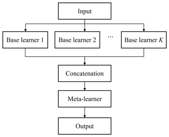
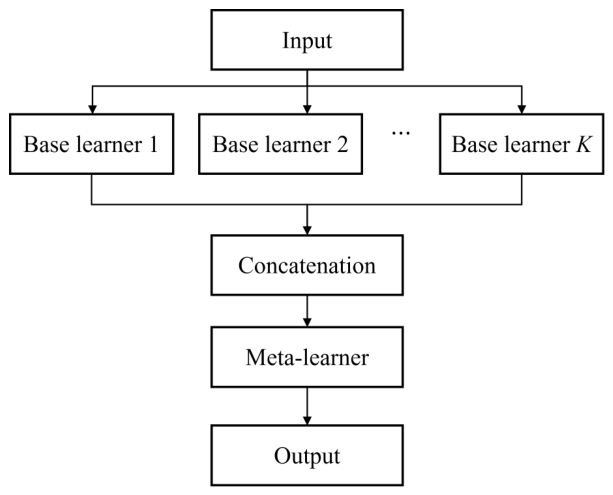
Stacking ensemble learning uses a two-level architecture comprising multiple base learners and one meta-learner. With a corresponding two-stage training strategy, it exploits complementary information among model predictions to improve overall predictive performance [40,41]. Its general architecture is shown in Figure 1.

Figure 1. General architecture of stacking ensemble learning.

Let the first-level model library comprise K heterogeneous base learners, $F=\left\{f_1,f_2,\dots ,f_K\right\}$. Let the complete multi-sensor structural dynamic response within a window be $X\in {\mathrm{R}}^{C\times W}$, where C is the number of sensor locations and W is the window length. Define a binary observation mask $M\in {\{0,1\}}^{C\times W}$, where $M_{c,t}=1$ indicates an available response at sensor c and time t, and $M_{c,t}=0$ indicates a missing response. The incomplete observed response is

$$X^{\mathrm{obs}}=M\odot X,$$

(1)

where $\odot$ denotes element-wise multiplication. Data reconstruction estimates the true responses at positions indexed by $1-M$, while preserving original available observations and exploiting temporal dependencies and inter-sensor spatial associations. At the first level, the k-th base learner takes $X^{\mathrm{obs}}$ and M as inputs and generates candidate reconstructed data with the same dimension as the complete response:

$${\widehat{X}}^{\left(k\right)}=f_k\left(X^{\mathrm{obs}},M;{\theta }_k\right),k=1,2,\dots ,K,$$

(2)

where ${\theta }_k$ denotes the trainable parameters of the k-th base learner. Grouped out-of-fold predictions are used to construct second-level samples, so each first-level prediction is generated by a learner not trained on that sample. Predictions from different base learners are concatenated to form the meta-learner input:

$$Z_{\mathrm{stack}}=\mathrm{concat}\left[{\widehat{X}}^{\left(1\right)},{\widehat{X}}^{\left(2\right)},\dots ,{\widehat{X}}^{\left(K\right)}\right].$$

(3)

At the second level, a meta-learner with parameters $\phi$ is trained on these out-of-fold predictions to learn complementary relationships among candidate reconstructed data and generate a fused prediction:

$${\widehat{X}}_{\mathrm{stack}}=g_{\phi }\left(Z_{\mathrm{stack}}\right),$$

(4)

where $g_{\phi }(·)$ denotes the meta-learner mapping. After it is trained, all base learners are refitted on the complete training set and used with the fixed meta-learner for validation and testing. Reformulating the conventional stacking formulation described above, the proposed framework incorporates grouped OOF predictions from the base learners for anchor selection, anchor-constrained residual meta-learning rather than direct complete-response prediction, and validation-gated fusion to regulate residual correction and final fusion. The following subsections describe these components.

2.2. Heterogeneous Base Learners and Anchor Selection

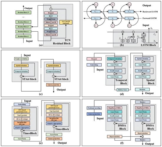
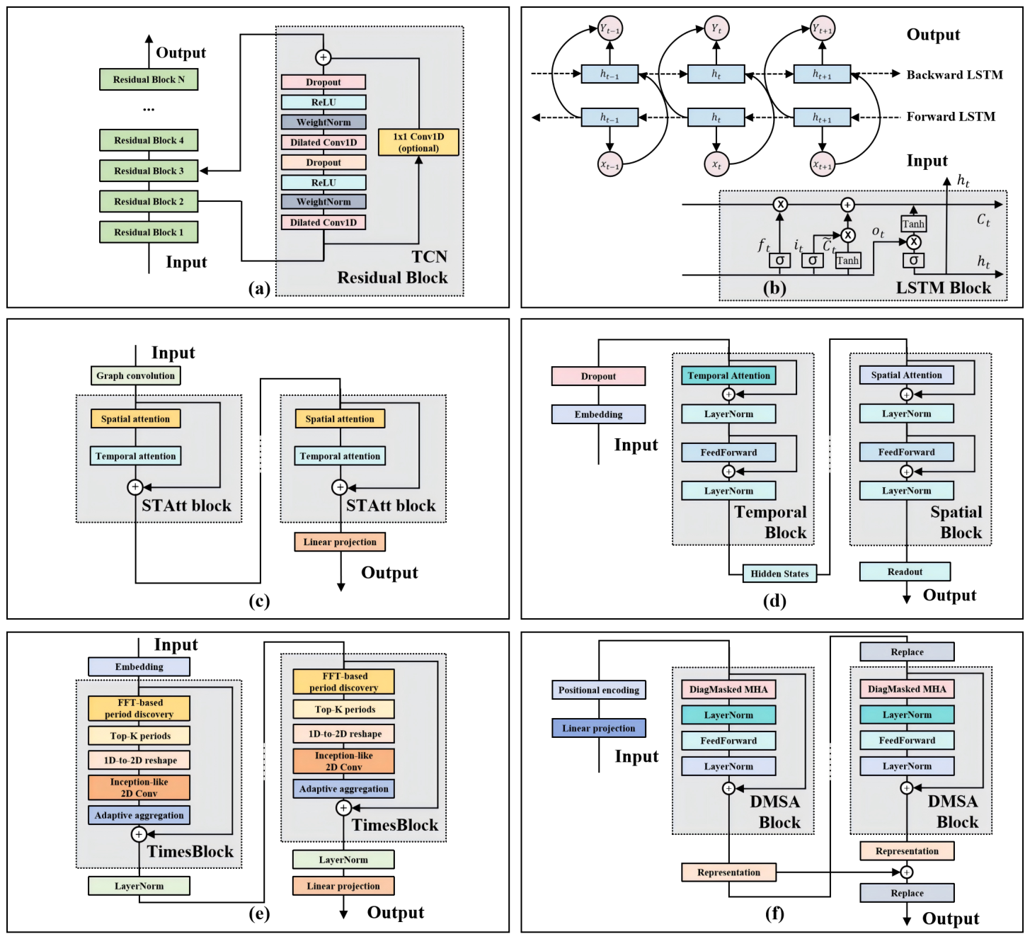
The effectiveness of Stacking depends on the reconstruction accuracy and error diversity of the base learners. The heterogeneous library includes TCN, BiLSTM, STGAT, ImputeFormer, TimesNet, and SAITS, as illustrated in Figure 2. The main architectural configurations and trainable parameter counts of the six base learners are summarized in Table 1. TCN uses dilated temporal convolutions and residual connections to capture long-range dependencies; BiLSTM combines forward and backward hidden states; STGAT combines graph-based spatial modeling with temporal dependency learning; ImputeFormer jointly models incomplete spatiotemporal sequences through temporal and spatial interactions; TimesNet identifies dominant periods and extracts intra- and inter-period variations through two-dimensional multiscale convolutions; and SAITS employs diagonally masked self-attention (DMSA) blocks and a weighted combination mechanism for multivariate time-series imputation. These models provide complementary temporal convolution, bidirectional recurrence, graph-based spatiotemporal modeling, low-rank spatiotemporal interaction, multi-period modeling, and self-attention-based imputation capabilities for subsequent meta-learning [8,21,23,30,31,32].

Figure 2. Architectures of the six heterogeneous base learners: (a) TCN, (b) BiLSTM, (c) STGAT, (d) ImputeFormer, (e) TimesNet, and (f) SAITS.

Table 1. Main architectural configurations of the six heterogeneous base learners.

Base Learner	Core Module	Depth	Dimensions	Key Architectural Settings	Parameters
TCN	TCN Residual Block	4	Hidden $=128$	Kernel $=3$; dilations $=\{1,2,4,8\}$; WeightNorm	406,942
BiLSTM	LSTM Block	3	Hidden $=256$	Bidirectional; concatenated features	4,428,182
STGAT	STAtt Block	2	Hidden $=64$	Heads = 4; dual-path graph; gated temporal convolution	127,297
ImputeFormer	Temporal BlockSpatial Block	3	Model $=192$	FFN $=384$; heads $=6$; rank $=32$	921,500
TimesNet	TimesBlock	2	Model $=64$	FFN $=128$; top-$k=3$; kernels $=\{1,3,5\}$	1,154,142
SAITS	DMSA Block	2	Model $=128$	FFN $=256$; heads $=4$; two-stage DMSA	556,006

Each base learner takes the incomplete response $X^{\mathrm{obs}}$ and observation mask M as inputs and outputs candidate reconstructed data ${\widehat{X}}^{\left(k\right)}$ with the same dimension as the complete response, as defined in Equation (2). The training loss of the k-th base learner is

$$l_{\mathrm{base}}^{\left(k\right)}={\displaystyle \frac{{∥(1-M)\odot \left({\widehat{X}}^{\left(k\right)}-X\right)∥}_1}{{∥1-M∥}_1+ϵ}}+{\lambda }_k{l}_{\mathrm{aux}}^{\left(k\right)},$$

(5)

The fractional term is a normalized $L_1$ reconstruction loss evaluated only at missing positions, and $ϵ$ is a small constant that prevents division by zero. $l_{\mathrm{aux}}^{\left(k\right)}$ denotes an auxiliary loss used by a specific base learner and ${\lambda }_k$ its weight; ${\lambda }_k=0$ for models without an auxiliary loss.

To prevent anchor selection and meta-learner training from using in-sample base-learner predictions, grouped three-fold out-of-fold prediction is performed on the first-level training set $D_B$. Based on original experimental records or contiguous time sources, $D_B$ is divided into Q non-overlapping groups:

$$D_B={\displaystyle \bigcup _{q=1}^Q}{G}_q,G_q\cap G_r=⌀,q\ne r,$$

(6)

where $Q=3$. All sliding windows generated from the same original record or contiguous time segment are assigned to one group, preventing highly overlapping windows from entering both fitting and holdout groups. In the q-th out-of-fold round, $G_q$ is held out and the k-th base learner is trained on the other $Q-1$ groups, yielding parameters ${\theta }_k^{(-q)}$. The fitted model then generates predictions for $G_q$:

$${\widehat{X}}_q^{\left(k\right)}=f_k\left(X_q^{\mathrm{obs}},M_q;{\theta }_k^{(-q)}\right),$$

(7)

where ${\theta }_k^{(-q)}$ denotes parameters trained without group q. After all folds are completed, predictions from the holdout groups are restored to their original sample indices in $D_B$, yielding the out-of-fold predictions of the k-th base learner over the full training set:

$${\widehat{X}}^{\left(k\right)}=\mathrm{Reorder}\left[{\widehat{X}}_1^{\left(k\right)},{\widehat{X}}_2^{\left(k\right)},\dots ,{\widehat{X}}_Q^{\left(k\right)}\right].$$

(8)

The base learner with the lowest relative root mean square error (RRMSE) at missing positions in the training out-of-fold predictions is selected as the anchor learner:

$$a=\underset{k\in \{1,\dots ,K\}}{\arg \min }{RRMSE}_{{\mathsf{\Omega }}^{\mathrm{miss}}}\left(X,{\widehat{X}}^{\left(k\right)}\right),$$

(9)

where ${\mathsf{\Omega }}^{\mathrm{miss}}$ is the set of missing positions in the training samples. Equation (9) is applied independently to each missing pattern, yielding a pattern-specific anchor learner.

After selection, the out-of-fold prediction of the a-th base learner becomes the anchor prediction, ${\widehat{X}}_{\mathrm{anchor}}={\widehat{X}}^{\left(a\right)}$, and the remaining $K-1$ predictions are denoted by ${\left\{{\widehat{X}}^{\left(k\right)}\right\}}_{k\ne a}$. These predictions are used to construct residual meta-features and train ResidualMetaNet. For the subsequent validation-gated fusion, the mean prediction of all K base learners is retained as a parameter-free ensemble reference:

$${\widehat{X}}_{\mathrm{mean}}={\displaystyle \frac{1}{K}}{\displaystyle \sum _{k=1}^K}{\widehat{X}}^{\left(k\right)}.$$

(10)

The ensemble mean is used only as a reference in the final fusion, while the anchor prediction remains the basis for residual meta-learning.

2.3. Residual Meta-Learner and Validation-Gated Fusion

We first construct the meta-learner input features. To represent the complementary information provided by each non-anchor learner relative to the anchor prediction, the relative prediction difference of the k-th non-anchor learner is defined as $\Delta {\widehat{X}}^{\left(k\right)}={\widehat{X}}^{\left(k\right)}-{\widehat{X}}_{\mathrm{anchor}}$, where $k\ne a$. The pointwise standard deviation of the base-learner predictions, $D={\mathrm{Std}}_{k=1,\dots ,K}\left({\widehat{X}}^{\left(k\right)}\right)$ is used to characterize inter-model prediction disagreement, where $D\in {\mathrm{R}}^{C\times W}$; a larger value indicates more pronounced differences among base-learner predictions at the corresponding sensor and time instant. In addition to the observation mask M, the missing ratio of the current window $r_{\mathrm{miss}}$, the longest consecutive missing length normalized by the window length ${\tilde{l}}_{\mathrm{miss}}$, the number of failed full channels normalized by the number of sensors ${\tilde{n}}_{\mathrm{failed}}$, and a sensor-wise spatial missingness feature map $S\left(M\right)$ are extracted. Here, $S\left(M\right)$ is obtained by extending the missing ratio of each sensor along the time dimension. These statistics are expanded to the dimensions of the response matrix and concatenated along the feature dimension as $P\left(M\right)=\mathrm{concat}\left[r_{\mathrm{miss}}1,{\tilde{l}}_{\mathrm{miss}}1,{\tilde{n}}_{\mathrm{failed}}1,S\left(M\right)\right]$. The meta-learner input representation is therefore:

$$Z=\mathrm{concat}\left[{\widehat{X}}_{\mathrm{anchor}},{\left\{\Delta {\widehat{X}}^{\left(k\right)}\right\}}_{k\ne a},D,M,P\left(M\right)\right],$$

(11)

where all features are concatenated along the feature dimension. The anchor prediction ${\widehat{X}}_{\mathrm{anchor}}$ provides the baseline reconstruction; relative model differences ${\{\Delta {\widehat{X}}^{\left(k\right)}\}}_{k\ne a}$ and prediction disagreement D characterize complementarity and consistency among base learners; and the observation mask M and its statistical features $P\left(M\right)$ describe the spatiotemporal missingness state of the current data.

Rather than directly regenerating the complete structural response, the meta-learner learns the residual error not recovered by the anchor prediction. Its residual supervision target is defined as

$$R^{\ast }=X-{\widehat{X}}_{\mathrm{anchor}}.$$

(12)

During meta-learner training, ${\widehat{X}}_{\mathrm{anchor}}$ uses the out-of-fold anchor predictions generated in the preceding subsection, preventing the anchor learner’s fitting advantage on its own training samples from entering the residual target. ResidualMetaNet generates a candidate residual correction from the meta-features:

$$\widehat{R}=f_{\mathrm{meta}}\left(Z;{\theta }_{\mathrm{meta}}\right),$$

(13)

where ${\theta }_{\mathrm{meta}}$ denotes the meta-learner parameters, and $\widehat{R}\in {\mathrm{R}}^{C\times W}$ denotes the predicted residual at each sensor and time instant. ResidualMetaNet uses a lightweight two-dimensional convolutional architecture: two $3\times 5$ convolutional layers, Gaussian error linear unit activation, and Dropout2D sequentially extract local relationships across sensor and temporal dimensions; a $1\times 1$ convolution then maps the hidden features to a single-channel residual matrix. The meta-learner training loss is defined as

$$l_{\mathrm{meta}}={\displaystyle \frac{{\parallel (1-M)\odot \left(\widehat{R}-R^{\ast }\right)\parallel }_1}{{∥1-M∥}_1+ϵ}}.$$

(14)

This loss focuses meta-learner fitting on anchor-learner errors at missing positions, preventing available observations from dominating second-level training.

The magnitude of the residual correction produced by the meta-learner may vary with the validation-data distribution; because residual learning attempts to compensate for anchor errors, inaccurate residual estimation may introduce unnecessary corrections, and adding it in full to the anchor prediction can therefore cause overcorrection. The reserved validation data are divided into a fusion-search set $V_F$ and a gate-validation set $V_G$, which are used for coefficient selection and independent gain validation, respectively. The residual coefficient ${\gamma }_r$ first constrains the correction applied by ResidualMetaNet around the pattern-specific anchor prediction, preventing residual learning from introducing corrections that degrade the anchor reconstruction. The final-fusion coefficient ${\gamma }_f$ further constrains the contribution of the resulting candidate reconstruction to the final output, providing additional protection when the learned residual correction becomes unreliable under noisy observations or distribution variations.

For the first-stage residual constraint, a candidate coefficient is selected from ${\Gamma }_r=\{0,\Delta {\gamma }_r,2\Delta {\gamma }_r,\dots ,1\}$ using $V_F$:

$${\tilde{\gamma }}_r=\underset{\gamma \in {\Gamma }_r}{\arg \min }{\mathrm{RRMSE}}_{{\mathsf{\Omega }}_{V_F}^{\mathrm{miss}}}\left(X_{V_F},{\widehat{X}}_{\mathrm{anchor},V_F}+\gamma {\widehat{R}}_{V_F}\right),$$

(15)

where ${\mathsf{\Omega }}_{V_F}^{\mathrm{miss}}$ denotes the missing positions in $V_F$. The selected coefficient is then evaluated on $V_G$, which is excluded from coefficient selection. Let $G_r^{V_G}$ denote the relative RRMSE gain of the residual-corrected prediction over the anchor prediction on $V_G$, calculated as $G_r^{V_G}=(L_{\mathrm{anchor}}^{V_G}-L_r^{V_G})/(L_{\mathrm{anchor}}^{V_G}+ϵ)$, where $L_{\mathrm{anchor}}^{V_G}$ and $L_r^{V_G}$ are their corresponding RRMSE values. Given the minimum relative-gain threshold ${\tau }_{\mathrm{rel}}$, the validated residual coefficient is

$${\gamma }_r=\left\{\begin{array}{cc}{\tilde{\gamma }}_r,\hfill & G_r^{V_G}\ge {\tau }_{\mathrm{rel}},\hfill \\ 0,\hfill & G_r^{V_G}<{\tau }_{\mathrm{rel}}.\hfill \end{array}\right.$$

(16)

The resulting anchor-constrained candidate reconstruction is therefore:

$${\widehat{X}}_{\mathrm{cand}}={\widehat{X}}_{\mathrm{anchor}}+{\gamma }_r\widehat{R}.$$

(17)

When ${\gamma }_r=1$, the full residual correction is applied to the anchor prediction; when ${\gamma }_r=0$, the residual correction is disabled and the candidate reconstruction reduces to the anchor prediction, while intermediate values scale the correction accordingly.

A second-stage constraint is then applied to the resulting candidate reconstruction. For this stage, the ensemble mean defined in Equation (10) serves as a parameter-free consensus reference to further verify whether the anchor-constrained candidate provides a reliable improvement beyond the first-stage residual correction before final fusion. From ${\Gamma }_f=\{0,\Delta {\gamma }_f,2\Delta {\gamma }_f,\dots ,1\}$, $V_F$ selects the candidate final-fusion coefficient:

$${\tilde{\gamma }}_f=\underset{\gamma \in {\Gamma }_f}{\arg \min }{\mathrm{RRMSE}}_{{\mathsf{\Omega }}_{V_F}^{\mathrm{miss}}}\left(X_{V_F},{\widehat{X}}_{\mathrm{mean},V_F}+\gamma \left({\widehat{X}}_{\mathrm{cand},V_F}-{\widehat{X}}_{\mathrm{mean},V_F}\right)\right).$$

(18)

Similarly, let $G_f^{V_G}$ denote the relative RRMSE gain of the candidate fusion over the ensemble reference on $V_G$, calculated as $G_f^{V_G}=(L_{\mathrm{mean}}^{V_G}-L_f^{V_G})/(L_{\mathrm{mean}}^{V_G}+ϵ)$. The validated final-fusion coefficient is

$${\gamma }_f=\left\{\begin{array}{cc}{\tilde{\gamma }}_f,\hfill & G_f^{V_G}\ge {\tau }_{\mathrm{rel}},\hfill \\ 0,\hfill & G_f^{V_G}<{\tau }_{\mathrm{rel}}.\hfill \end{array}\right.$$

(19)

The search step sizes were set to $\Delta {\gamma }_r=\Delta {\gamma }_f=0.05$, and the relative-gain threshold was fixed at ${\tau }_{\mathrm{rel}}=0.001$ to exclude negligible validation gains while retaining effective fusion corrections. Thus, both coefficients follow the same validation protocol: $V_F$ determines the candidate coefficient, whereas $V_G$ independently verifies whether the corresponding fusion provides sufficient reconstruction gain. The two coefficients act at different levels: ${\gamma }_r$ constrains the residual correction around the anchor prediction, whereas ${\gamma }_f$ constrains the contribution of the resulting candidate reconstruction to the final output. The final validation-gated reconstruction is

$${\widehat{X}}_{\mathrm{safe}}={\widehat{X}}_{\mathrm{mean}}+{\gamma }_f\left({\widehat{X}}_{\mathrm{cand}}-{\widehat{X}}_{\mathrm{mean}}\right).$$

(20)

When ${\gamma }_f=1$, the validated anchor-constrained candidate is fully retained; when ${\gamma }_f=0$, the prediction reverts to the ensemble reference, while intermediate values provide a constrained transition between the candidate reconstruction and the ensemble reference.

Consequently, the first-stage constraint preserves the anchor-constrained nature of residual stacking, while the second-stage constraint provides an additional safeguard against unreliable candidate reconstructions caused by noise interference or distribution variations.

2.4. Computational Procedure

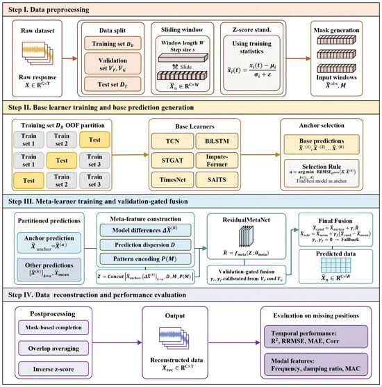
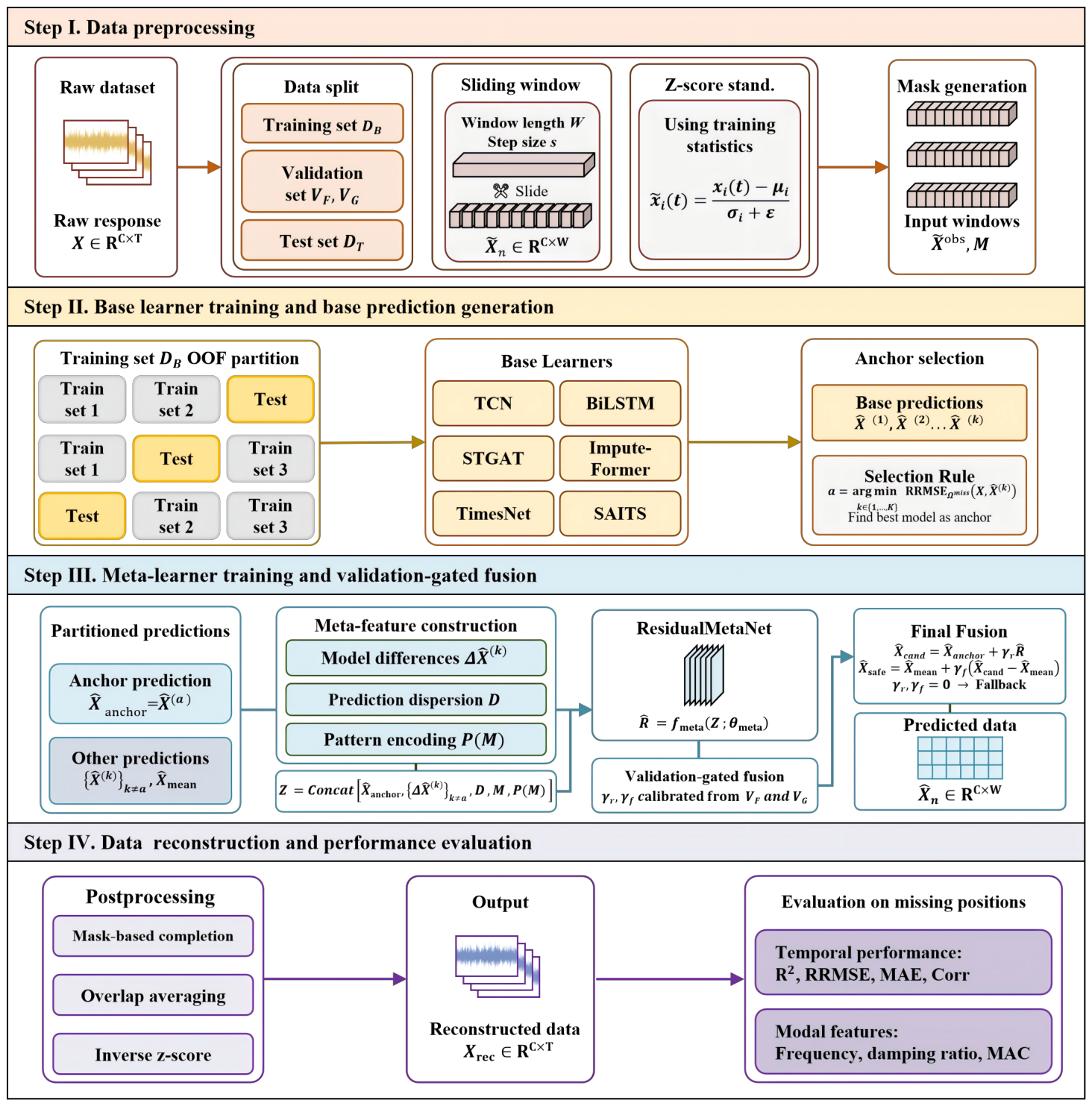
The complete computational procedure is shown in Figure 3. It comprises data preprocessing; base-learner training and base prediction generation; residual meta-learner training and validation-gated fusion; and data reconstruction and performance evaluation.

Figure 3. Overall computational procedure of the proposed method.

• Step I: Data preprocessing.

This step corresponds to Step I in Figure 3. The raw structural responses are first divided into a first-level training set $D_B$, fusion-search set $V_F$, gate-validation set $V_G$, and final test set $D_T$. $D_B$ trains the base learners and residual meta-learner; $V_F$ is used for candidate-coefficient selection; $V_G$ independently verifies whether the selected coefficients provide sufficient reconstruction gain; and $D_T$ is reserved exclusively for final performance evaluation.

Within each subset, windowed samples are constructed with a sliding window of length W and step size s. The complete response window X, observation mask M, and incomplete input $X^{\mathrm{obs}}$ are generated as defined above. Window-position indices in the original time series are retained for subsequent aggregation of overlapping windows.

To reduce the effect of response-amplitude differences across sensors on model training, each sensor response is standardized using Z-score normalization:

$${\tilde{x}}_i\left(t\right)={\displaystyle \frac{x_i\left(t\right)-{\mu }_i}{{\sigma }_i+ϵ}},$$

(21)

where $x_i\left(t\right)$ and ${\tilde{x}}_i\left(t\right)$ are the original and standardized responses of sensor i at time t, respectively; ${\mu }_i$ and ${\sigma }_i$ are its mean and standard deviation in the training data; and $ϵ$ is a small constant that prevents division by zero. The parameters computed from $D_B$ are fixed for $V_F$, $V_G$, and $D_T$; during grouped out-of-fold prediction, the parameters for each fold are calculated only from its fitting groups.

• Step II: Base learner training and base prediction generation.

This stage takes X, M, and $X^{\mathrm{obs}}$ in $D_B$ as inputs. As shown in Step II of Figure 3, the training samples are divided into three non-overlapping groups. In each round, two groups train every base learner and out-of-fold predictions are generated for the held-out group. After three rounds, held-out predictions are restored to the original sample order, yielding first-level predictions from all base learners over $D_B$, ${\left\{{\widehat{X}}^{\left(k\right)}\right\}}_{k=1}^K$.

The model with the best overall reconstruction performance, based on RRMSE at missing positions in the training samples, is selected as the anchor learner; its prediction is denoted by ${\widehat{X}}_{\mathrm{anchor}}={\widehat{X}}^{\left(a\right)}$, and the remaining base-learner predictions are denoted by ${\left\{{\widehat{X}}^{\left(k\right)}\right\}}_{k\ne a}$. The out-of-fold first-level predictions are used to train the residual meta-learner in the next stage. Meanwhile, the base learners are refitted on complete $D_B$ to generate final predictions on $V_F$, $V_G$, and $D_T$. This stage determines anchor index a and yields the anchor and non-anchor predictions.

• Step III: Meta-learner training and validation-gated fusion.

This stage takes the anchor prediction ${\widehat{X}}_{\mathrm{anchor}}$, non-anchor predictions ${\left\{{\widehat{X}}^{\left(k\right)}\right\}}_{k\ne a}$, the ensemble mean ${\widehat{X}}_{\mathrm{mean}}$, and observation mask M as inputs. As shown in Step III of Figure 3, the differences $\Delta {\widehat{X}}^{\left(k\right)}$ between non-anchor and anchor predictions, together with the pointwise model disagreement D, are first calculated. The missing ratio, longest consecutive missing length, number of failed full channels, and spatial distribution of missingness are also extracted from the observation mask. These inputs are concatenated along the feature dimension to form the meta-learner input Z in Equation (11).

The meta-learner uses the difference between the complete response and anchor prediction as its residual target and optimizes its parameters only at missing positions according to Equation (14). After meta-learner training, the fully trained base learners and meta-learner are applied to $V_F$ and $V_G$. The residual coefficient ${\gamma }_r$ is first selected on $V_F$ and validated on $V_G$ to constrain the residual correction around the anchor prediction, yielding the candidate reconstruction ${\widehat{X}}_{\mathrm{cand}}={\widehat{X}}_{\mathrm{anchor}}+{\gamma }_r\widehat{R}$. The final-fusion coefficient ${\gamma }_f$ is then selected and validated using the same $V_F$-selection and $V_G$-validation protocol to constrain the contribution of the candidate reconstruction to the final output.

The validation-gated window-level fusion prediction is

$$\widehat{X}={\widehat{X}}_{\mathrm{mean}}+{\gamma }_f\left({\widehat{X}}_{\mathrm{anchor}}+{\gamma }_r\widehat{R}-{\widehat{X}}_{\mathrm{mean}}\right).$$

(22)

This stage yields the validated coefficients ${\gamma }_r$ and ${\gamma }_f$ and the window-level fusion prediction $\widehat{X}\in {\mathrm{R}}^{C\times W}$ required for subsequent response reconstruction.

• Step IV: Data reconstruction and performance evaluation.

This stage takes the window-level fusion prediction $\widehat{X}$, incomplete input $X^{\mathrm{obs}}$, observation mask M, window-position indices, and training-set normalization parameters as inputs. Corresponding to Step IV in Figure 3, it completes missing positions, aggregates overlapping windows, reverses normalization, and evaluates performance. For the n-th window, the fusion prediction obtained in Step III is denoted by ${\widehat{X}}_n\in {\mathrm{R}}^{C\times W}$. Applying the fusion prediction only at missing positions gives the completed window response:

$$X_{\mathrm{comp},n}=X_n^{\mathrm{obs}}+(1-M_n)\odot {\widehat{X}}_n,$$

(23)

where $X_{\mathrm{comp},n}\in {\mathrm{R}}^{C\times W}$ is the completed result for the n-th window. Because $X_n^{\mathrm{obs}}=M_n\odot X_n$, Equation (23) preserves the original response at observed positions and applies model predictions only at missing positions.

To recover a continuous response from the window-level results, let the first sample of the n-th window in the original time series be ${\tau }_n=(n-1)s+1$, where s is the sliding step size. For sample $\tau$ in the original time series, the set of windows covering this position is denoted by ${\mathsf{\Omega }}_{\tau }=\left\{n\mid {\tau }_n\le \tau \le {\tau }_n+W-1\right\}$. The continuous aggregated response on the standardized scale is

$$X_{\mathrm{agg}}(i,\tau )={\displaystyle \frac{1}{\left|{\mathsf{\Omega }}_{\tau }\right|}}\sum _{n\in {\mathsf{\Omega }}_{\tau }}{X}_{\mathrm{comp},n}\left(i,\tau -{\tau }_n+1\right),i=1,\dots ,C,\tau =1,\dots ,T,$$

(24)

where $\tau -{\tau }_n+1$ is the local time index of original position $\tau$ in the n-th window. Averaging predictions from overlapping windows reduces the effect of prediction fluctuations near window boundaries on the continuous reconstructed response.

The continuous response is then returned to the original physical scale using the means and standard deviations calculated from the training set:

$$X_{\mathrm{rec}}(i,\tau )=({\sigma }_i+ϵ)X_{\mathrm{agg}}(i,\tau )+{\mu }_i,$$

(25)

where ${\mu }_i$ and ${\sigma }_i$ are the mean and standard deviation, respectively, of sensor i in the training data. The resulting continuous reconstructed response is $X_{\mathrm{rec}}\in {\mathrm{R}}^{C\times T}$.

Model performance is evaluated only at positions where the reference response is valid but marked as missing by the observation mask, thereby reflecting the ability to reconstruct missing structural dynamic responses. The coefficient of determination ($R^2$), relative root mean square error (RRMSE), mean absolute error (MAE), and Pearson correlation coefficient (Corr) are used to quantify time-domain agreement between the reconstructed and reference responses, as defined below:

$$R^2=1-{\displaystyle \frac{{\sum }_{m=1}^{N_{\mathrm{mis}}}{\left(x_m-{\widehat{x}}_m\right)}^2}{{\sum }_{m=1}^{N_{\mathrm{mis}}}{\left(x_m-\overline{x}\right)}^2}},$$

(26)

$$RRMSE=\sqrt{{\displaystyle \frac{{\sum }_{m=1}^{N_{\mathrm{mis}}}{\left(x_m-{\widehat{x}}_m\right)}^2}{{\sum }_{m=1}^{N_{\mathrm{mis}}}{x}_m^2}}},$$

(27)

$$\mathrm{MAE}={\displaystyle \frac{1}{N_{\mathrm{mis}}}}{\displaystyle \sum _{m=1}^{N_{\mathrm{mis}}}}\left|x_m-{\widehat{x}}_m\right|,$$

(28)

$$\mathrm{Corr}={\displaystyle \frac{{\sum }_{m=1}^{N_{\mathrm{mis}}}\left(x_m-\overline{x}\right)\left({\widehat{x}}_m-\overline{\widehat{x}}\right)}{\sqrt{{\sum }_{m=1}^{N_{\mathrm{mis}}}{\left(x_m-\overline{x}\right)}^2}\sqrt{{\sum }_{m=1}^{N_{\mathrm{mis}}}{\left({\widehat{x}}_m-\overline{\widehat{x}}\right)}^2}}},$$

(29)

where $N_{\mathrm{mis}}$ is the number of valid missing entries included in evaluation; $x_m$ and ${\widehat{x}}_m$ are the reference and reconstructed responses at the m-th missing position; and $\overline{x}$ and $\overline{\widehat{x}}$ are their respective means over all valid missing positions. Higher $R^2$ and Corr and lower RRMSE and MAE indicate better reconstruction performance. Operational modal analysis is further performed to assess the preservation of principal structural dynamic characteristics in terms of natural frequencies, damping ratios, mode shapes, and the modal assurance criterion (MAC).

3. Real Bridge Application and Validation

3.1. Bridge Overview and Its Diverse Pattern Missing Data

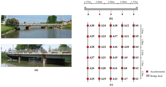
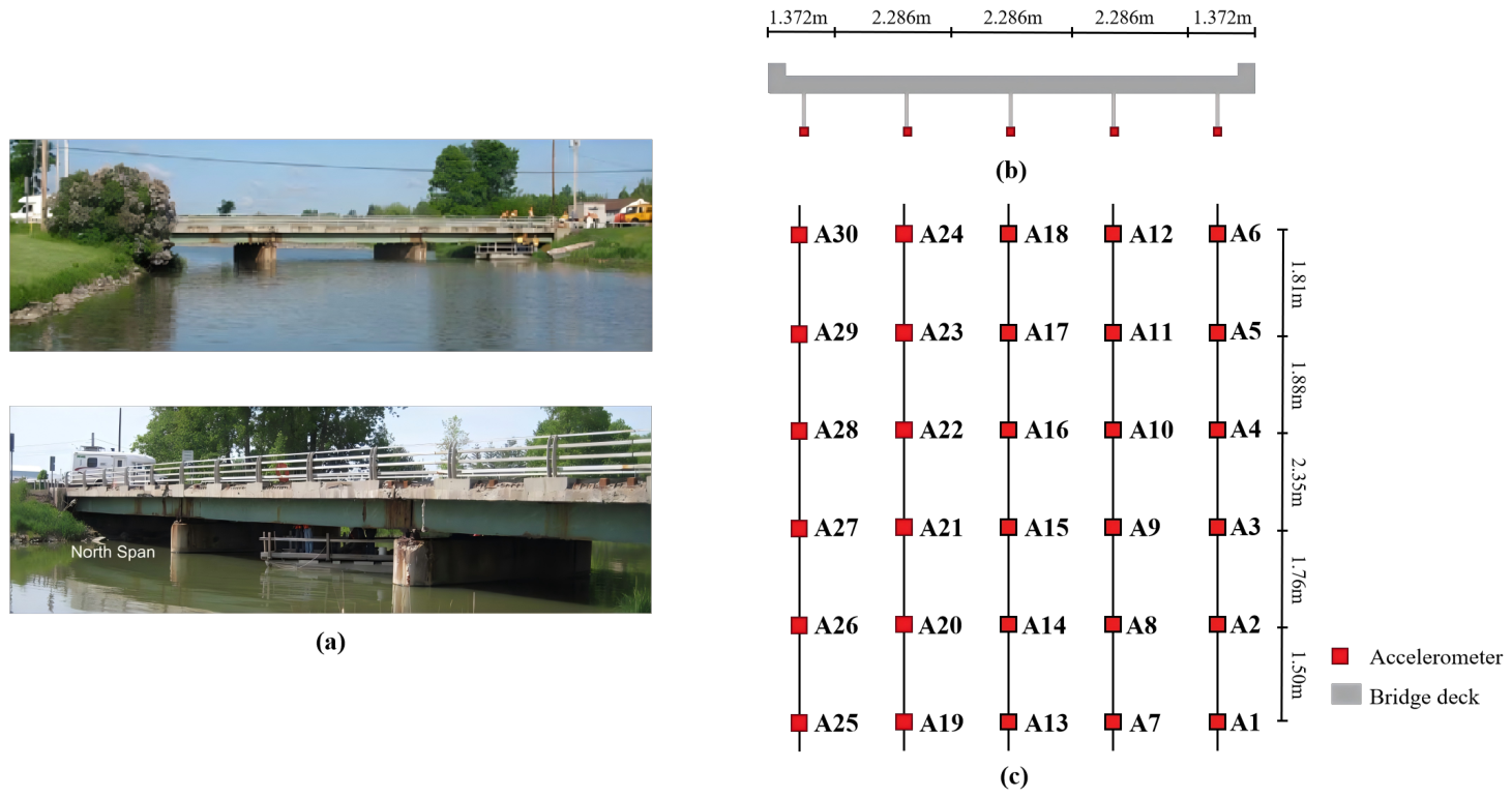
To validate reconstruction under different structural states, the proposed method is evaluated using a bridge subjected to structural-state tests [47,48]. The test structure is a steel stringer bridge in Waddington, NY, USA, comprising three independent simply supported spans with a cast-in-place reinforced-concrete deck supported by steel stringers. The bridge was constructed in 1957 and had been in service for approximately 51 years at the time of the test program. The superstructure consisted of a 190 mm-thick reinforced-concrete deck supported by two exterior W840 × 210 (W33 × 141) and three interior W840 × 226 (W33 × 152) steel stringers, with a center-to-center spacing of approximately 2.1 m [48,49]. The north span was selected for testing. It has a rocker expansion bearing at one end and a fixed bearing at the other, with a center-to-center span length of 13.716 m. A biennial inspection conducted approximately six months before the test program rated the deck, superstructure, and substructure as poor, good, and fair, respectively, with reported deterioration including heavy deck efflorescence, localized spalling of the sidewalk and fascia, joint leakage and corrosion, and rocker-bearing corrosion [48]. Field testing was conducted before demolition, and different structural states were created by imposing bearing displacements and removing diaphragm-connection bolts. Thirty biaxial accelerometers were uniformly deployed along the five stringers of the north span, with six sensors on each stringer, numbered A01–A30. The vertical z-direction acceleration recorded by all 30 sensors was used as model input. Figure 4 shows the bridge, cross-section, and sensor layout.

Figure 4. Overview of the steel stringer bridge and accelerometer layout: (a) general view of the bridge, (b) cross-section of the monitored north span, and (c) plan view of the accelerometer layout.

In the field dynamic tests, bridge responses were excited by a heavy maintenance vehicle with a wheelbase of 7.87 m and track width of 2.29 m. Vibration data were collected under eight structural states including two baseline states and six damage states, as described in Table 2. The response data were segmented into windows of length 256 with a step size of 64, corresponding to a 2 s duration and 0.5 s shift at 128 Hz. The first three structural states formed $D_B$ for training the base learners and meta-learner, comprising 1590 windows. Damage 2 was reserved for validation, of which 156 windows were used for $V_F$ for coefficient selection, 27 windows served as a separation segment between $V_F$ and $V_G$, and 165 windows were used for $V_G$ for independent gain confirmation. The separation segment was excluded from coefficient selection and gain confirmation. Damage 3–Damage 6 constituted $D_T$ for final testing, comprising 2288 windows. Grouped three-fold OOF splitting was performed using the original records in the training set, ensuring that overlapping windows generated from the same record remained within the same fold and preventing information leakage between training and holdout folds. All responses were standardized using Z-score normalization, with the means and standard deviations calculated only from the complete training set and then fixed for validation and testing.

Table 2. Structural states and data partitioning for the steel stringer bridge.

State	Structural Condition	Description	Data Partition
Baseline 1	Initial baseline state	Structural response before imposed damage	Training
Baseline 2	Second baseline state	Baseline response reacquired after removing hydraulic jacks near the bearing	Training
Damage 1	Bearing displacement	Approximately 3 mm vertical displacement imposed near the rocker bearing	Training
Damage 2	Bearing displacement	Approximately 5 mm vertical displacement imposed near the rocker bearing	Validation
Damage 3	Interior diaphragm-connection damage	Removal of four of the six bolts at one connection	Testing
Damage 4	Interior diaphragm-connection damage	Removal of the remaining two bolts at the same connection	Testing
Damage 5	Cumulative multi-connection damage	Removal of all six bolts at another interior diaphragm connection	Testing
Damage 6	End-diaphragm connection damage	Removal of all six bolts at an end diaphragm connection	Testing

Three missing patterns were considered to represent different temporal and spatial forms of data loss: Random missing, Channel missing, and Block missing. They represent scattered packet loss, complete sensor-channel loss, and consecutive localized data loss, respectively. A 40% temporal missing level was adopted for Random missing and for the affected channels in Block missing as a challenging partial-loss condition. Within each structural state and sub-pattern, all six base learners used the same observation mask to ensure a fair comparison. For Random missing, approximately 40% of the temporal samples were randomly masked across all 30 sensor channels, and three realizations generated using fixed random seeds were independently evaluated. For Channel missing, each sensor channel was treated as fully missing in turn, resulting in 30 single-sensor-failure sub-patterns. For Block missing, 15 longitudinally adjacent sensor pairs were considered, with each pair subjected to a consecutive missing segment covering 40% of the response duration. The same sensor-pair configuration and generation rule were used across the four test structural states. Results within each missing pattern were equally averaged over the corresponding sub-patterns. The three missing patterns are summarized in Table 3.

Table 3. Missing-data patterns considered in the steel stringer bridge.

Missing Pattern	Missing Setting	Engineering Interpretation
Random missing	40% random missing data across all sensors	Random packet loss
Channel missing	Full-channel missing of individual sensors	Sensor failure
Block missing	40% consecutive missing data in adjacent sensor pairs	Link interruption

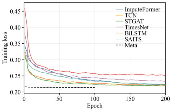
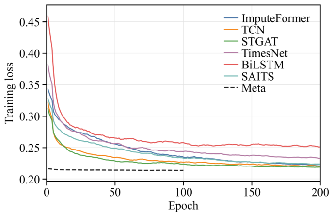
The heterogeneous base learners described in Section 2.2 were used in the case study. The anchor learner was selected during the training stage based on the grouped OOF results on $D_B$. STGAT achieved the lowest OOF RRMSE for all three missing patterns and was therefore used as the anchor learner for Random, Channel, and Block missing. The meta-learner was trained to correct residual errors in the anchor prediction at missing positions. All models were implemented in Python 3.12 with PyTorch 2.8.0 and CUDA 12.8 and trained on an NVIDIA GeForce RTX 4090 GPU (NVIDIA Corporation, Santa Clara, CA, USA), with a 16-vCPU Intel Xeon Platinum 8352V CPU (Intel Corporation, Santa Clara, CA, USA) and 120 GB RAM. AdamW was used with learning rates of $1\times {10}^{-3}$ and $5\times {10}^{-4}$ for the base learners and meta-learner, respectively, and a weight decay of $1\times {10}^{-4}$; the base learners and meta-learner were trained for 200 and 100 epochs. Figure 5 shows the training loss curves of the base learners and the meta-learner. The validation-gain criterion was satisfied under all three missing patterns.

Figure 5. Training loss curves of the base learners and meta-learner for the steel stringer bridge.

3.2. Data Reconstruction and Time Domain Performance

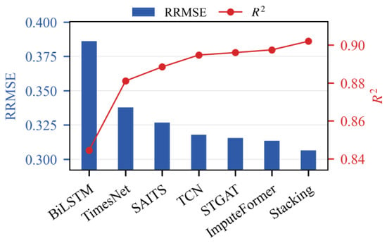
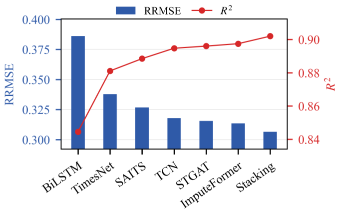
The proposed method was then evaluated on the final test set. Table 4 summarizes the mean reconstruction performance across four test structural states, and Figure 6 compares the mean $R^2$ and RRMSE among methods. ImputeFormer achieves the highest $R^2$ and Corr and the lowest RRMSE among the six base learners, whereas STGAT gives the lowest MAE. Stacking further improves the mean $R^2$ and Corr to 0.9020 and 0.9496 and reduces RRMSE and MAE to 0.3065 and 0.1523. Compared with the best corresponding base learner results, Stacking improves $R^2$ by 0.0046 and Corr by 0.0024, while reducing RRMSE by approximately 2.26% and MAE by 1.99%. These results indicate that Stacking can effectively exploit complementary information among heterogeneous base learners.

Table 4. Overall data reconstruction performance of the base learners and Stacking for the steel stringer bridge.

Method	${\mathit{R}}^2$	RRMSE	MAE	Corr
BiLSTM	0.8445	0.3861	0.1847	0.9184
TimesNet	0.8811	0.3379	0.1659	0.9384
SAITS	0.8885	0.3267	0.1612	0.9426
TCN	0.8947	0.3178	0.1579	0.9457
STGAT	0.8960	0.3155	0.1554	0.9464
ImputeFormer	0.8974	0.3136	0.1559	0.9472
Stacking	0.9020	0.3065	0.1523	0.9496

Figure 6. Comparison of mean $R^2$ and RRMSE among the base learners and Stacking for the steel stringer bridge.

To further examine whether the reconstruction improvement is maintained across different structural states, Table 5 compares the performance of the Anchor learner and Stacking across Damage 3–Damage 6. For each structural state, the reported metrics are obtained by equal-weight averaging over the Random, Channel, and Block missing patterns. Stacking consistently improves upon the Anchor learner in all four states, with RRMSE reductions ranging from 2.26% to 3.44%, indicating that the reconstruction improvement is maintained across structural states with different reconstruction difficulty.

Table 5. Reconstruction performance of the Anchor learner and Stacking across different structural states for the steel stringer bridge.

Damage State	Method	${\mathit{R}}^2$	RRMSE	MAE	Corr	RRMSE Improvement
Damage 3	Anchor	0.9148	0.2852	0.1579	0.9562	2.54%
	Stacking	0.9188	0.2780	0.1543	0.9584
Damage 4	Anchor	0.9043	0.3026	0.1597	0.9507	2.59%
	Stacking	0.9090	0.2948	0.1558	0.9532
Damage 5	Anchor	0.8921	0.3217	0.1608	0.9442	2.26%
	Stacking	0.8968	0.3144	0.1574	0.9467
Damage 6	Anchor	0.8674	0.3534	0.1439	0.9342	3.44%
	Stacking	0.8783	0.3413	0.1419	0.9389

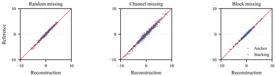
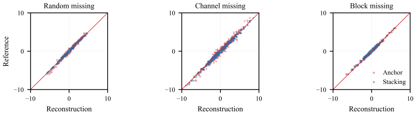
Table 6 shows that Stacking outperforms the anchor learner under Random missing, Channel missing, and Block missing, increasing $R^2$ and Corr while reducing RRMSE and MAE. These results indicate that the temporal, spatial, and global dependencies captured by heterogeneous base learners effectively complement the anchor prediction and provide stable residual corrections in challenging cases such as full-channel failure and consecutive block missingness. Figure 7 further shows closer agreement between responses reconstructed by Stacking and the reference responses, consistent with the quantitative results.

Table 6. Data reconstruction performance of the anchor learner and Stacking under different missing patterns for the steel stringer bridge.

Missing Pattern	Method	${\mathit{R}}^2$	RRMSE	MAE	Corr	RRMSE Improvement
Random missing	Anchor	0.9086	0.3023	0.1544	0.9532	3.34%
	Stacking	0.9146	0.2922	0.1509	0.9564
Channel missing	Anchor	0.8832	0.3268	0.1539	0.9392	2.21%
	Stacking	0.8889	0.3196	0.1518	0.9423
Block missing	Anchor	0.8962	0.3175	0.1580	0.9467	3.09%
	Stacking	0.9024	0.3077	0.1540	0.9500

Figure 7. Agreement between reference data and reconstructed data of the anchor learner and Stacking under different missing patterns for the steel stringer bridge.

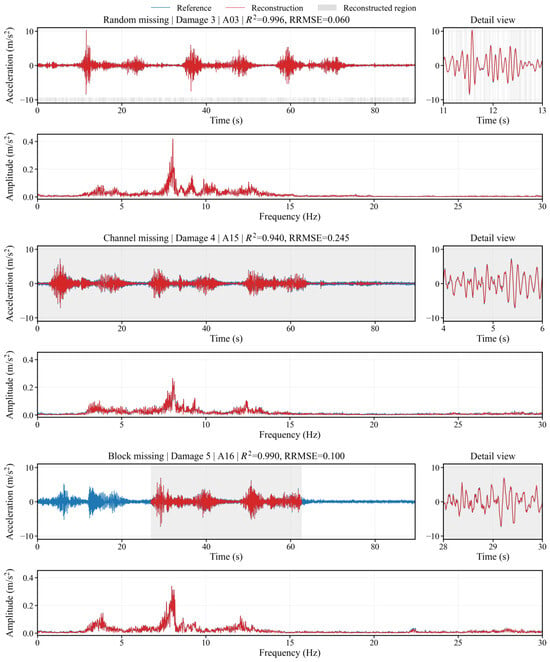
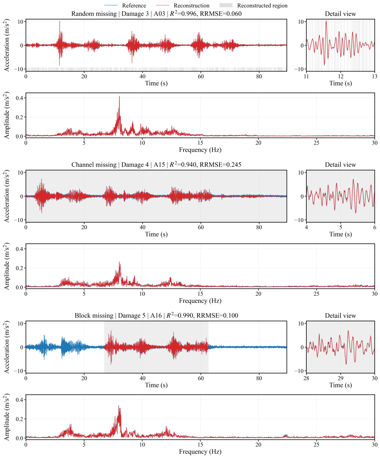
Figure 8 presents representative time- and frequency-domain reconstruction results under the three missing patterns. The three cases were selected as representative examples to illustrate the reconstruction behavior under different missing patterns and structural states, and the spectra were computed after inverse normalization to the original physical scale. Stacking closely reproduces the main waveform variations of the reference responses, while the local detail views further show good agreement in the reconstructed segments.

Figure 8. Representative reconstruction results of Stacking under different missing patterns for the steel stringer bridge.

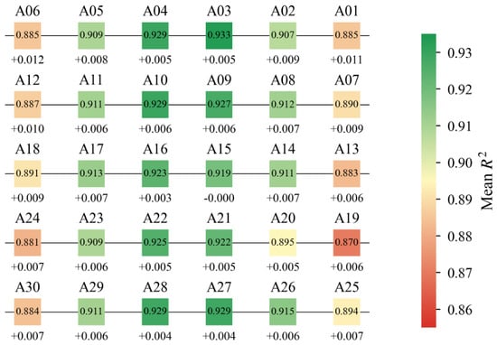
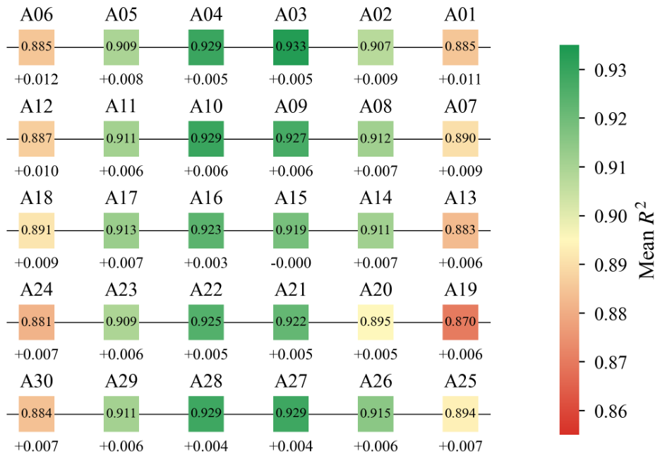
Figure 9 further presents the mean $R^2$ at individual sensors and the corresponding reconstruction gains of Stacking over the anchor learner. For each sensor, the reported values were averaged over all test structural states, the three missing patterns, and the corresponding subcases involving that sensor. The reported gain represents the mean increase in $R^2$ achieved by Stacking relative to the Anchor learner. The anchor reconstruction accuracy varies across sensor locations, indicating spatial differences in reconstruction difficulty across the monitored bridge. Despite this variation, positive gains are observed at different sensor locations and are broadly distributed across different stringers and bridgewise positions, showing that the improvement of Stacking is not confined to a few specific regions. Together with the results under the three missing patterns and four structural states, these findings support the stable reconstruction performance of the proposed method.

Figure 9. Mean $R^2$ and data reconstruction improvement from the anchor learner to Stacking at different sensors for the steel stringer bridge.

3.3. Ablation Analysis

To examine the contribution of the main components of the proposed method, ablation experiments were conducted by selectively removing the anchor constraint, grouped OOF prediction strategy, and validation-gated fusion, together with SimpleMean as a basic ensemble reference. The corresponding variants and their settings are summarized in Table 7. All variants use the same data partition, missing patterns, and evaluation protocol to ensure a consistent comparison.

Table 7. Ablation settings of the proposed Stacking framework.

Variant	Setting	Purpose
SimpleMean	Average of all base-learner predictions	Compare with simple ensemble fusion
Anchor	Anchor learner only	Single-learner reference
w/o Anchor	Meta-learning without anchor constraint	Anchor-constrained residual learning
w/o OOF	In-sample predictions for meta-learner	Assess grouped OOF prediction strategy
w/o gated fusion	Without validation-gated fusion	Assess validation-gated fusion
Stacking	Complete proposed method	Evaluate the combined framework

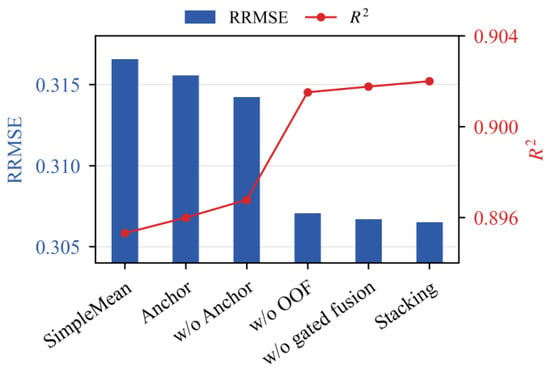
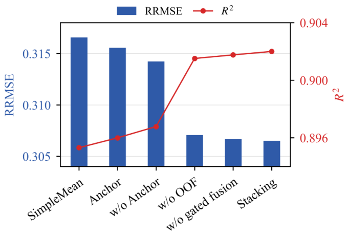
As shown in Table 8 and Figure 10, the complete method achieves the best overall performance, with the highest $R^2$ and Corr and the lowest RRMSE and MAE. Removing the anchor constraint causes a clear performance degradation, confirming that anchor-constrained residual learning provides an effective basis for the meta-learner and prevents unnecessary modification of well-reconstructed responses. Removing grouped OOF prediction also leads to a slight but consistent decrease in reconstruction accuracy, indicating that out-of-fold predictions improve the reliability of second-level learning by reducing optimistic fitting effects. Validation-gated fusion further contributes to the reconstruction performance, while its role in improving robustness is assessed in the subsequent noise-robustness analysis. In addition, Stacking clearly outperforms SimpleMean and the anchor prediction, demonstrating that the proposed framework can effectively exploit complementary information among heterogeneous base learners rather than relying on simple averaging or a single strong learner.

Table 8. Reconstruction performance of different ablation variants for the steel stringer bridge.

Method	${\mathit{R}}^2$	RRMSE	MAE	Corr
SimpleMean	0.8953	0.3165	0.1568	0.9462
Anchor	0.8960	0.3155	0.1554	0.9464
w/o Anchor	0.8968	0.3142	0.1554	0.9471
w/o OOF	0.9015	0.3070	0.1526	0.9493
w/o gated fusion	0.9017	0.3067	0.1524	0.9494
Stacking	0.9020	0.3065	0.1523	0.9496

Figure 10. Comparison of mean $R^2$ and RRMSE among the ablation variants for the steel stringer bridge.

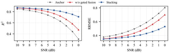
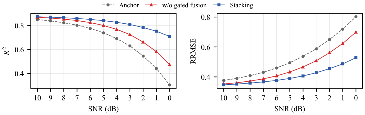
To evaluate noise robustness and the effect of the gated fusion, zero-mean Gaussian white noise was added to the observed responses under the Random missing pattern at signal-to-noise ratio (SNR) levels from 10 to 0 dB. All base learners and the meta-learner were trained on noise-free data and kept fixed, while the two gated-fusion coefficients were recalibrated for each SNR level using the corresponding noisy validation data. Three independent noise realizations were generated at each level and the results were averaged. In addition to the complete Stacking method, an ungated variant was constructed by setting both fusion coefficients to unity (${\gamma }_r$ = ${\gamma }_f$ = 1), while keeping the base learners, meta-learner, and all other settings unchanged. The anchor learner was also included as a reference.

As shown in Table 9 and Figure 11, reconstruction performance decreases for all schemes as the noise level increases. Stacking consistently outperforms both the ungated variant and the anchor prediction over the entire range. Compared with the ungated variant, the $R^2$ improvement increases from 0.53% at 10 dB to 49.62% at 0 dB, while the corresponding RRMSE reduction increases from 1.65% to 24.41%. Moreover, the performance gap becomes increasingly pronounced as the noise level increases. These results demonstrate that gated fusion effectively limits performance degradation under noisy observations. By controlling the contribution of the residual-based candidate reconstruction, the final-fusion constraint reduces the influence of noise-amplified residual errors and improves the robustness of the proposed Stacking method.

Table 9. Comparison of reconstruction performance with and without gated fusion under different SNR levels for the steel stringer bridge.

SNR (dB)	${\mathit{R}}^2$					RRMSE
	w/o Gated	Stacking	ΔR2	Improvement		w/o Gated	Stacking	ΔRRMSE	Reduction
10	0.8675	0.8721	0.0046	0.53%		0.3529	0.3471	0.0058	1.65%
9	0.8614	0.8684	0.0070	0.81%		0.3609	0.3521	0.0088	2.41%
8	0.8522	0.8635	0.0113	1.32%		0.3725	0.3589	0.0136	3.66%
7	0.8404	0.8576	0.0172	2.05%		0.3870	0.3668	0.0202	5.21%
6	0.8234	0.8500	0.0266	3.24%		0.4069	0.3768	0.0301	7.39%
5	0.7998	0.8397	0.0399	5.00%		0.4329	0.3899	0.0430	9.94%
4	0.7670	0.8260	0.0590	7.68%		0.4665	0.4066	0.0599	12.84%
3	0.7234	0.8075	0.0841	11.62%		0.5077	0.4279	0.0798	15.72%
2	0.6612	0.7826	0.1214	18.36%		0.5611	0.4551	0.1060	18.90%
1	0.5818	0.7515	0.1697	29.18%		0.6229	0.4869	0.1360	21.84%
0	0.4733	0.7081	0.2348	49.62%		0.6987	0.5281	0.1706	24.41%

Figure 11. Noise robustness comparison of different reconstruction schemes for the steel stringer bridge.

3.4. Frequency Domain Performance

To examine the preservation of structural dynamic characteristics, operational modal analysis was conducted under the Channel missing pattern in the test set using both the complete reference responses and responses reconstructed by Stacking. The reconstructed response of each individually missing sensor was concatenated across all sensors to form a complete multichannel response for modal identification. The first six modes were identified using covariance-driven stochastic subspace identification (SSI-COV). For SSI-COV, a fourth-order zero-phase Butterworth band-pass filter over 3–32 Hz, 44 block rows, and model orders of 60–120 was used. Stable poles were retained with damping ratios below 18% and eigenvalue moduli below 1.02. The reconstructed responses were evaluated in terms of modal frequencies, damping ratios, and the modal assurance criterion (MAC), as summarized in Table 10.

Table 10. Comparison of modal parameters identified from the reference and reconstructed responses for the steel stringer bridge.

Mode	Frequency/Hz				Damping Ratio/%			MAC
	Reference	Reconstructed	Error/%		Reference	Reconstructed	Error/%
1st	7.9393	7.9927	0.6722		2.6858	2.9411	9.5068	0.9967
2nd	10.2207	10.2268	0.0599		2.7838	2.4300	12.7097	0.9997
3rd	12.0002	11.9329	0.5607		2.1056	2.2640	7.5222	0.9913
4th	18.6567	18.7624	0.5666		3.0781	2.4808	19.4054	0.9953
5th	24.9213	24.9223	0.0040		0.7626	0.9931	30.2246	0.9815
6th	28.0147	27.9371	0.2770		2.8044	3.0609	9.1439	0.9763

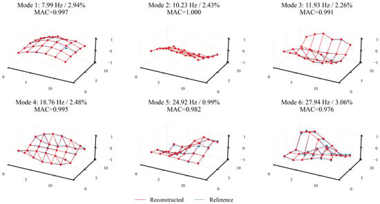
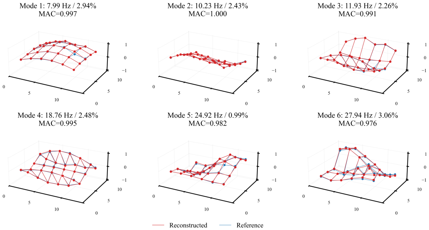
Table 10 shows that the modal frequencies identified from the reconstructed responses remain in close agreement with those obtained from the reference responses. The frequency errors of the first six modes remain below 0.68%, indicating close agreement between the modal frequencies identified from the reconstructed and reference responses. In contrast, the damping ratios exhibit greater sensitivity to reconstruction errors, with larger deviations observed in several modes, particularly the fourth and fifth modes. Despite these differences, the MAC remain high, ranging from 0.9763 to 0.9997, indicating strong consistency between the reconstructed and reference mode shapes. These results suggest that Stacking effectively preserves the principal modal frequencies and spatial mode-shape characteristics under Channel missing, whereas damping-ratio estimation is comparatively more sensitive to local reconstruction errors and response variations. Figure 12 further confirms the overall agreement between the reconstructed and reference mode shapes.

Figure 12. Comparison of the first six reference and reconstructed mode shapes for the steel stringer bridge.

4. Conclusions

This study proposes an anchor-constrained residual stacking method for structural dynamic-response data reconstruction. The proposed method integrates heterogeneous base learners, grouped OOF anchor selection, residual meta-learning, and validation-gated fusion to exploit complementary information among base learners while limiting unreliable residual and fusion contributions. The method is evaluated using monitoring data from a steel stringer bridge under multiple structural states. The main conclusions are as follows:

(1) The proposed method improves overall data reconstruction performance by exploiting information from heterogeneous base learners. It achieves the best overall performance among the compared methods, with an $R^2$ of 0.9020 and an RRMSE of 0.3065, an MAE of 0.1523, and a Corr of 0.9496, demonstrating improved reconstruction performance over individual base learners.

(2) The proposed method provides consistent reconstruction gains under different missing patterns, reducing RRMSE by 3.34%, 2.21%, and 3.09%, respectively, relative to the corresponding anchor learner. The improvements are also maintained across the four test structural states, with RRMSE reductions ranging from 2.26% to 3.44%. Ablation results further confirm the contributions of anchor-constrained residual learning, grouped OOF prediction, and validation-gated fusion. Under measurement noise, Stacking consistently outperforms the variant without gated fusion, with the advantage becoming more pronounced as SNR decreases, demonstrating the robustness of validation-gated fusion under noisy observations. These results support reliable recovery of incomplete monitoring data under varying missing and noisy conditions, thereby providing a more reliable basis for subsequent SHM analysis.

(3) Modal analysis results confirm that the reconstructed responses preserve the principal modal characteristics of the structure. For the steel stringer bridge under Channel missing, the frequency errors of the first six modes remain below 0.68%, and the MAC remain above 0.9763. Although damping-ratio estimates are more sensitive to reconstruction errors, the reconstructed responses maintain good agreement in modal frequencies and mode shapes, providing reliable data support for subsequent modal analysis and structural condition assessment.

Although the proposed method demonstrates consistent improvements across different missing patterns and structural states, the current validation-gated fusion relies on prespecified gain thresholds and discrete searches for the residual and final-fusion coefficients. Future research will investigate adaptive coefficient calibration, uncertainty-aware fusion, and broader validation using long-term monitoring data from different structural systems.

References

- Farrar, C.R.; Worden, K. An introduction to structural health monitoring. Philos. Trans. R. Soc. A Math. Phys. Eng. Sci. 2007, 365, 303–315. [Google Scholar] [CrossRef] [Scilit]
- Brownjohn, J.M.W. Structural health monitoring of civil infrastructure. Philos. Trans. R. Soc. A Math. Phys. Eng. Sci. 2007, 365, 589–622. [Google Scholar] [CrossRef] [Scilit]
- Li, Z.; Lin, W.; Kim, C.W.; Limongelli, M.P.; Chatzi, E. A comprehensive review of indirect bridge health monitoring. Mech. Syst. Signal Process. 2026, 247, 113918. [Google Scholar] [CrossRef] [Scilit]
- Spencer, B.F.; Ruiz-Sandoval, M.E.; Kurata, N. Smart sensing technology: Opportunities and challenges. Struct. Control Health Monit. 2004, 11, 349–368. [Google Scholar] [CrossRef] [Scilit]
- Abdulkarem, M.; Samsudin, K.; Rokhani, F.Z.; Rasid, M.F.A. Wireless sensor network for structural health monitoring: A contemporary review of technologies, challenges, and future direction. Struct. Health Monit. 2020, 19, 693–735. [Google Scholar] [CrossRef] [Scilit]
- Zhang, J.; Huang, M.; Wan, N.; Deng, Z.; He, Z.; Luo, J. Missing measurement data recovery methods in structural health monitoring: The state, challenges and case study. Measurement 2024, 231, 114528. [Google Scholar] [CrossRef] [Scilit]
- Lavassani, S.H.H.; Doroudi, R.; Shahrouzi, M.; Hejazi, F. A comprehensive method for sensor fault detection and signal reconstruction in structural health monitoring systems for super-tall buildings. Structures 2025, 75, 108866. [Google Scholar] [CrossRef] [Scilit]
- Niu, J.; Li, S.; Li, Z. Restoration of missing structural health monitoring data using spatiotemporal graph attention networks. Struct. Health Monit. 2022, 21, 2408–2419. [Google Scholar] [CrossRef] [Scilit]
- Zhang, Z.; Luo, Y. Restoring method for missing data of spatial structural stress monitoring based on correlation. Mech. Syst. Signal Process. 2017, 91, 266–277. [Google Scholar] [CrossRef] [Scilit]
- Li, L.; Liu, H.; Zhou, H.; Zhang, C. Missing data estimation method for time series data in structure health monitoring systems by probability principal component analysis. Adv. Eng. Softw. 2020, 149, 102901. [Google Scholar] [CrossRef] [Scilit]
- Ma, Z.; Luo, Y.; Yun, C.B.; Wan, H.P.; Shen, Y. An MPPCA-based approach for anomaly detection of structures under multiple operational conditions and missing data. Struct. Health Monit. 2023, 22, 1069–1089. [Google Scholar] [CrossRef] [Scilit]
- Yang, Y.; Nagarajaiah, S. Harnessing data structure for recovery of randomly missing structural vibration responses time history: Sparse representation versus low-rank structure. Mech. Syst. Signal Process. 2016, 74, 165–182. [Google Scholar] [CrossRef] [Scilit]
- Chen, S.Y.; Wang, Y.W.; Ni, Y.Q. Multi-channel lost data recovery for structural health monitoring by structured low-rank matrix completion. Struct. Health Monit. 2025. epub ahead of print. [Google Scholar] [CrossRef] [Scilit]
- Huang, Y.; Beck, J.L.; Wu, S.; Li, H. Bayesian compressive sensing for approximately sparse signals and application to structural health monitoring signals for data loss recovery. Probabilistic Eng. Mech. 2016, 46, 62–79. [Google Scholar] [CrossRef] [Scilit]
- Ren, P.; Chen, X.; Sun, L.; Sun, H. Incremental bayesian matrix/tensor learning for structural monitoring data imputation and response forecasting. Mech. Syst. Signal Process. 2021, 158, 107734. [Google Scholar] [CrossRef] [Scilit]
- Ye, X.; Su, Y.; Xi, P.; Liu, H. Structural health monitoring data reconstruction of a concrete cable-stayed bridge based on wavelet multi-resolution analysis and support vector machine. Comput. Concr. 2017, 20, 555–562. [Google Scholar] [CrossRef]
- Zhang, Y.M.; Wang, H.; Bai, Y.; Mao, J.X.; Xu, Y.C. Bayesian dynamic regression for reconstructing missing data in structural health monitoring. Struct. Health Monit. 2022, 21, 2097–2115. [Google Scholar] [CrossRef] [Scilit]
- Ma, Y.; He, Y.; Wang, L.; Zhang, J. Probabilistic reconstruction for spatiotemporal sensor data integrated with gaussian process regression. Probabilistic Eng. Mech. 2022, 69, 103264. [Google Scholar] [CrossRef] [Scilit]
- Oh, B.K.; Glisic, B.; Kim, Y.; Park, H.S. Convolutional neural network–based data recovery method for structural health monitoring. Struct. Health Monit. 2020, 19, 1821–1838. [Google Scholar] [CrossRef] [Scilit]
- Hochreiter, S.; Schmidhuber, J. Long short-term memory. Neural Comput. 1997, 9, 1735–1780. [Google Scholar] [CrossRef] [Scilit]
- Schuster, M.; Paliwal, K.K. Bidirectional recurrent neural networks. IEEE Trans. Signal Process. 1997, 45, 2673–2681. [Google Scholar] [CrossRef] [Scilit]
- Jeong, S.; Ferguson, M.; Hou, R.; Lynch, J.P.; Sohn, H.; Law, K.H. Sensor data reconstruction using bidirectional recurrent neural network with application to bridge monitoring. Adv. Eng. Inform. 2019, 42, 100991. [Google Scholar] [CrossRef] [Scilit]
- Bai, S.; Kolter, J.Z.; Koltun, V. An empirical evaluation of generic convolutional and recurrent networks for sequence modeling. arXiv 2018, arXiv:1803.01271. [Google Scholar] [CrossRef] [Scilit]
- Lei, X.; Sun, L.; Xia, Y. Lost data reconstruction for structural health monitoring using deep convolutional generative adversarial networks. Struct. Health Monit. 2021, 20, 2069–2087. [Google Scholar] [CrossRef] [Scilit]
- Gao, S.; Zhao, W.; Wan, C.; Jiang, H.; Ding, Y.; Xue, S. Missing data imputation framework for bridge structural health monitoring based on slim generative adversarial networks. Measurement 2022, 204, 112095. [Google Scholar] [CrossRef] [Scilit]
- Fan, G.; Li, J.; Hao, H.; Xin, Y. Data driven structural dynamic response reconstruction using segment based generative adversarial networks. Eng. Struct. 2021, 234, 111970. [Google Scholar] [CrossRef] [Scilit]
- Shu, J.; Yu, H.; Liu, G.; Duan, Y.; Hu, H.; Zhang, H. DF-CDM: Conditional diffusion model with data fusion for structural dynamic response reconstruction. Mech. Syst. Signal Process. 2025, 222, 111783. [Google Scholar] [CrossRef] [Scilit]
- Jiang, K.; Han, Q.; Du, X.; Ni, P. Structural dynamic response reconstruction and virtual sensing using a sequence to sequence modeling with attention mechanism. Autom. Constr. 2021, 131, 103895. [Google Scholar] [CrossRef] [Scilit]
- Yang, F.; Song, X.; Yi, W.; Li, R.; Wang, Y.; Xiao, Y.; Ma, L.; Ma, X. Lost data reconstruction for structural health monitoring by parallel mixed transformer-CNN network. Mech. Syst. Signal Process. 2025, 224, 112142. [Google Scholar] [CrossRef] [Scilit]
- Nie, T.; Qin, G.; Ma, W.; Mei, Y.; Sun, J. ImputeFormer: Low rankness-induced transformers for generalizable spatiotemporal imputation. In Proceedings of the 30th ACM SIGKDD Conference on Knowledge Discovery and Data Mining; ACM: New York, NY, USA, 2024; pp. 2260–2271. [Google Scholar] [CrossRef] [Scilit]
- Du, W.; Côté, D.; Liu, Y. SAITS: Self-attention-based imputation for time series. Expert Syst. Appl. 2023, 219, 119619. [Google Scholar] [CrossRef] [Scilit]
- Wu, H.; Hu, T.; Liu, Y.; Zhou, H.; Wang, J.; Long, M. TimesNet: Temporal 2D-variation modeling for general time series analysis. In Proceedings of the International Conference on Learning Representations, Kigali, Rwanda, 1–5 May 2023. [Google Scholar]
- Bloemheuvel, S.; van den Hoogen, J.; Atzmueller, M. A computational framework for modeling complex sensor network data using graph signal processing and graph neural networks in structural health monitoring. Appl. Netw. Sci. 2021, 6, 97–120. [Google Scholar] [CrossRef] [Scilit]
- Liu, P.; Tang, Z.; Zhang, C.; Huang, X.; Xu, W. Nonuniform data loss reconstruction based on time-series-specialized neural networks for structural health monitoring. Struct. Health Monit. 2026, 25, 2262–2286. [Google Scholar] [CrossRef] [Scilit]
- Zheng, W.; Li, J.; Hao, H.; Fan, G. Missing data imputation for structural health monitoring using unsupervised domain adaptation and pretraining techniques. Eng. Struct. 2025, 328, 119694. [Google Scholar] [CrossRef] [Scilit]
- Zhang, M.; Guo, T.; Zhang, G.; Liu, Z.; Liu, Y. Missing monitoring data reconstruction for cable-stayed bridge using knowledge transfer-based generative pre-trained model. Struct. Health Monit. 2025. epub ahead of print. [Google Scholar] [CrossRef] [Scilit]
- Clemen, R.T. Combining forecasts: A review and annotated bibliography. Int. J. Forecast. 1989, 5, 559–583. [Google Scholar] [CrossRef] [Scilit]
- Brown, G.; Wyatt, J.; Harris, R.; Yao, X. Diversity creation methods: A survey and categorisation. Inf. Fusion 2005, 6, 5–20. [Google Scholar] [CrossRef]
- Wang, X.; Hyndman, R.J.; Li, F.; Kang, Y. Forecast combinations: An over 50-year review. Int. J. Forecast. 2023, 39, 1518–1547. [Google Scholar] [CrossRef] [Scilit]
- Wolpert, D.H. Stacked generalization. Neural Netw. 1992, 5, 241–259. [Google Scholar] [CrossRef] [Scilit]
- Breiman, L. Stacked regressions. Mach. Learn. 1996, 24, 49–64. [Google Scholar] [CrossRef] [Scilit]
- van der Laan, M.J.; Polley, E.C.; Hubbard, A.E. Super learner. Stat. Appl. Genet. Mol. Biol. 2007, 6, 25. [Google Scholar] [CrossRef] [Scilit]
- Oliveira, M.; Torgo, L. Ensembles for time series forecasting. In Proceedings of the Sixth Asian Conference on Machine Learning; PMLR: Cambridge, MA, USA, 2015; Volume 39, pp. 360–370. [Google Scholar]
- Moon, J.; Jung, S.; Rew, J.; Rho, S.; Hwang, E. Combination of short-term load forecasting models based on a stacking ensemble approach. Energy Build. 2020, 216, 109921. [Google Scholar] [CrossRef] [Scilit]
- Hasson, H.; Maddix, D.C.; Wang, B.; Gupta, G.; Park, Y. Theoretical guarantees of learning ensembling strategies with applications to time series forecasting. In Proceedings of the 40th International Conference on Machine Learning; PMLR: Cambridge, MA, USA, 2023; Volume 202, pp. 12616–12632. [Google Scholar]
- Bergmeir, C.; Benítez, J.M. On the use of cross-validation for time series predictor evaluation. Inf. Sci. 2012, 191, 192–213. [Google Scholar] [CrossRef] [Scilit]
- Whelan, M.J.; Janoyan, K.D. In-service diagnostics of a highway bridge from a progressive damage case study. J. Bridge Eng. 2010, 15, 597–607. [Google Scholar] [CrossRef] [Scilit]
- Whelan, M.; Gangone, M.; Janoyan, K. Data Set from Ambient Vibration Monitoring and Static Loading of a Steel Stringer Bridge Subject to Imposed Damage; Zenodo: Geneva, Switzerland, 2025. [Google Scholar] [CrossRef]
- Whelan, M.J.; Janoyan, K.D. Design of a Robust, High-Rate Wireless Sensor Network for Static and Dynamic Structural Health Monitoring. J. Intell. Mater. Syst. Struct. 2009, 20, 849–863. [Google Scholar] [CrossRef] [Scilit]
Disclaimer/Publisher’s Note: The statements, opinions and data contained in all publications are solely those of the individual author(s) and contributor(s) and not of MDPI and/or the editor(s). MDPI and/or the editor(s) disclaim responsibility for any injury to people or property resulting from any ideas, methods, instructions or products referred to in the content. |
© 2026 by the authors. Licensee MDPI, Basel, Switzerland. This article is an open access article distributed under the terms and conditions of the Creative Commons Attribution (CC BY) license.