


Abstract
Bond strength degradation of corroded reinforced concrete (RC) structures involves complex mechanical interactions that are difficult to capture through experimental or purely data-driven methods alone. This study proposes a physics-informed neural network (PINN) framework that embeds a thin-walled cylinder rust expansion model as differentiable soft constraints in the loss function, achieving deep integration of mechanical priors with data-driven learning. The PINN predicts the bond strength τu alongside intermediate physical quantities including rust expansion stress σr, hoop stress σθ, and damage variable Dθ. A four-stage progressive training strategy is adopted to balance data fitting and physical consistency. The results show that the proposed PINN improves R2 by 5.49–15.66% and reduces SMAPE by 33.91–58.87% compared to XGBoost, RF, and SVM, while achieving an average prediction error of 1.66% in experimental validation. Under the cover thickness extrapolation scenario (15 mm → 10 mm), the PINN maintains prediction errors within 1.5%, significantly outperforming both ML models and empirical formulas. The framework’s interpretability is further demonstrated through decomposition of the bond strength into frictional and mechanical interlock components, providing mechanistic insight into the corrosion-induced failure process.
1. Introduction
Reinforced concrete is the dominant structural material worldwide, a status attributable to its superior mechanical performance, the accessibility of its constituent materials, and its economic advantages [1,2,3,4]. Bond strength is a critical factor governing the failure of reinforced concrete (RC) structures. Corrosion of steel reinforcement reduces the bar cross-section, generates expansive stresses that crack the concrete cover, and ultimately degrades the steel–concrete bond interface, compromising structural performance [5,6,7,8]. Accurately predicting the bond strength of corroded RC members is challenging, as it depends on multiple interacting parameters—including corrosion rate, concrete compressive strength, bar diameter, bond length, yield strength, and cover thickness [9,10,11].
Researchers have analyzed the bond strength of corroded RC components based on electrochemical reaction mechanisms. In terms of theoretical models [12,13], some scholars have established calculation models of bond strength of RC members under different corrosion forms (uniform corrosion and non-uniform corrosion) based on elastic-plastic theory and thin-walled cylinder theory. In terms of the empirical formula [14,15], other researchers have developed bond strength models for corroded reinforced concrete through data fitting based on experimental studies. In terms of numerical simulation [16], scholars have further elucidated the bond degradation mechanism of corroded RC members by considering the transport of corrosive media in concrete and the effects of electrochemical reactions. However, the simplifications and assumptions inherent in mechanism-driven models often limit their predictive accuracy and general applicability.
Advances in computer technology have established machine learning as an effective approach for tackling high-dimensional problems and achieving high-precision predictions [17,18,19,20]. Mousavi et al. [21] investigated the ultimate and relative bond strength between corroded rebars and concrete, with and without transverse rebars, using MLP, RBFNN, and SVR techniques. The effects of concrete compressive strength, steel yield strength, and corrosion rate were studied using random forest (RF) methods [22]. Using 268 sets of existing test data and a range of machine learning models, Mohseni [23] established predictive frameworks for the bond strength of both FRP and steel bars in concrete. MEI [24] developed a probabilistic prediction model for bond strength at high temperatures using the NGBoost method, which demonstrated superior predictive accuracy compared to empirical formulas.
However, these machine learning models present the following limitations: (1) they only learn the relationship between inputs and outputs from the training data without considering the underlying physical laws, so prediction quality depends entirely on the quantity and quality of the data; and (2) they are primarily applicable to interpolation within the dataset and perform poorly on samples that fall outside the data range. Unlike fully data-driven machine learning models, the PINN is driven by both data and physical knowledge. By incorporating physical equations, boundary conditions, and initial conditions to describe the problem, the model can make predictions based on known physical laws, thereby significantly improving prediction accuracy [25].
Physics-informed neural networks (PINNs) overcome these limitations by embedding physical equations as soft constraints in the loss function, enabling predictions that are simultaneously data-consistent and physically plausible [26]. However, existing PINN applications in structural engineering predominantly adopt generic frameworks with simple elasticity or diffusion equations [27,28], which cannot capture the complex mechanical behavior of corrosion-induced bond degradation-particularly the non-uniform rust expansion pressure and the nonlinear degradation of interfacial friction and mechanical interlocking.
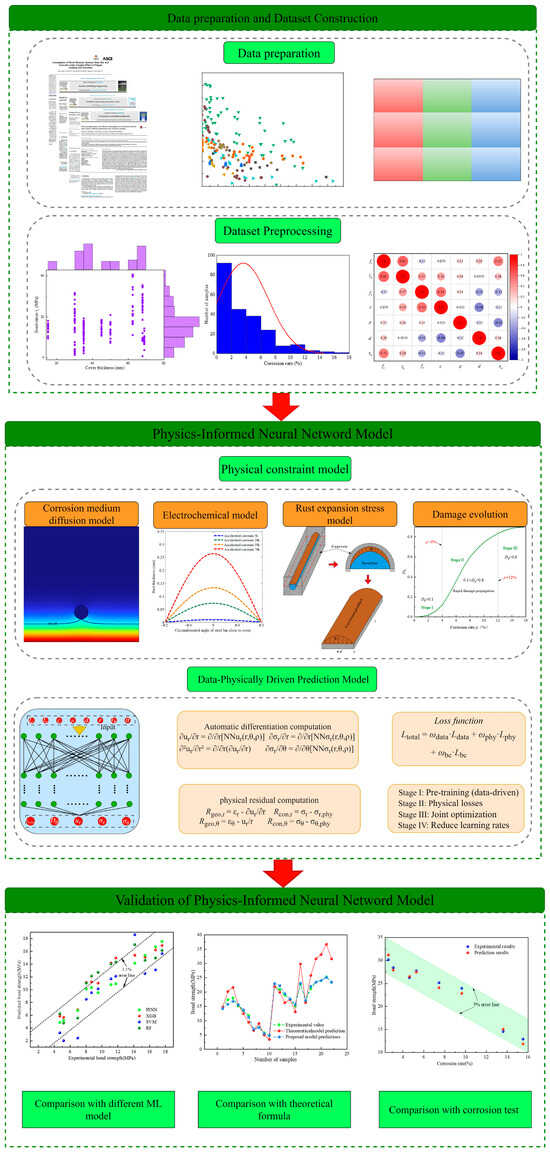
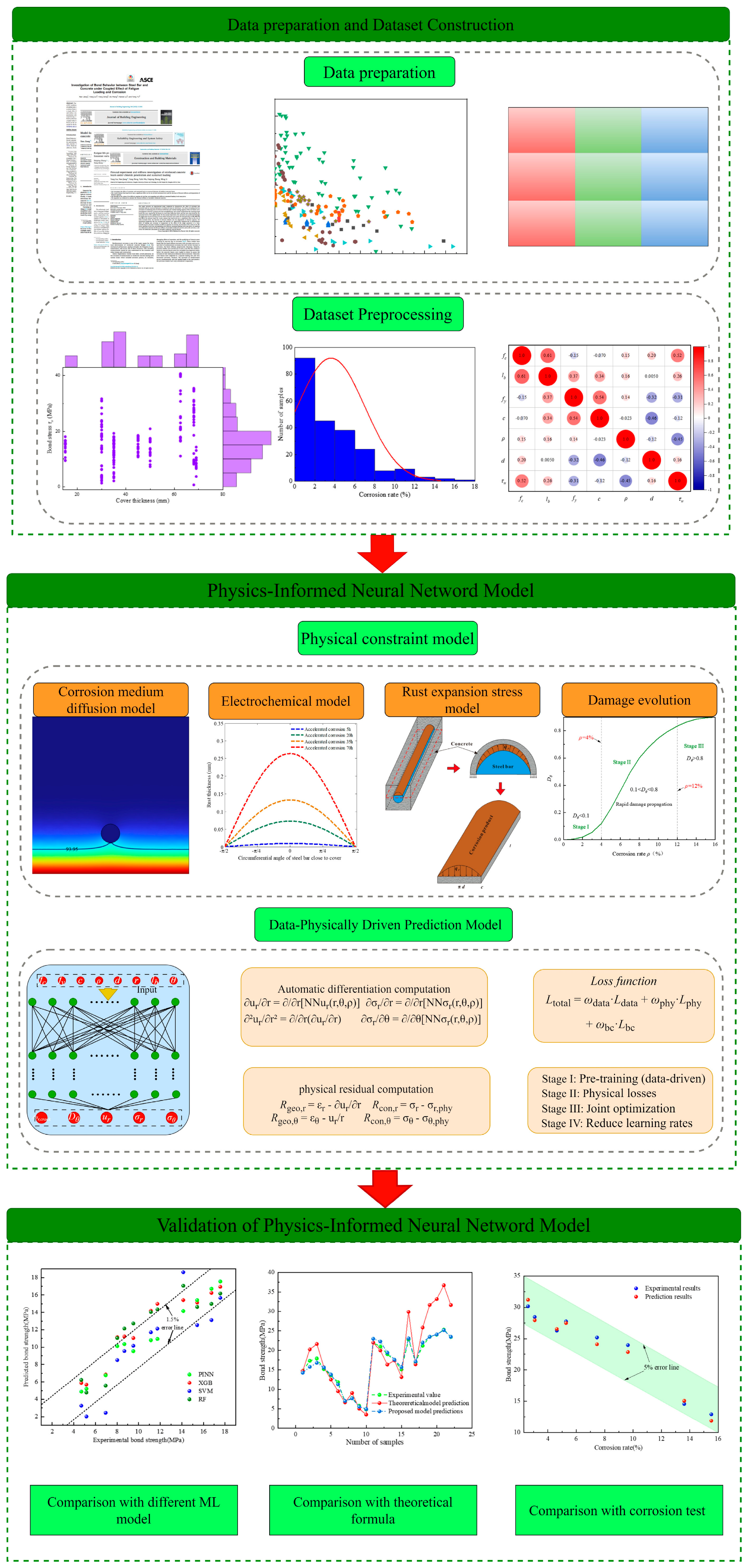
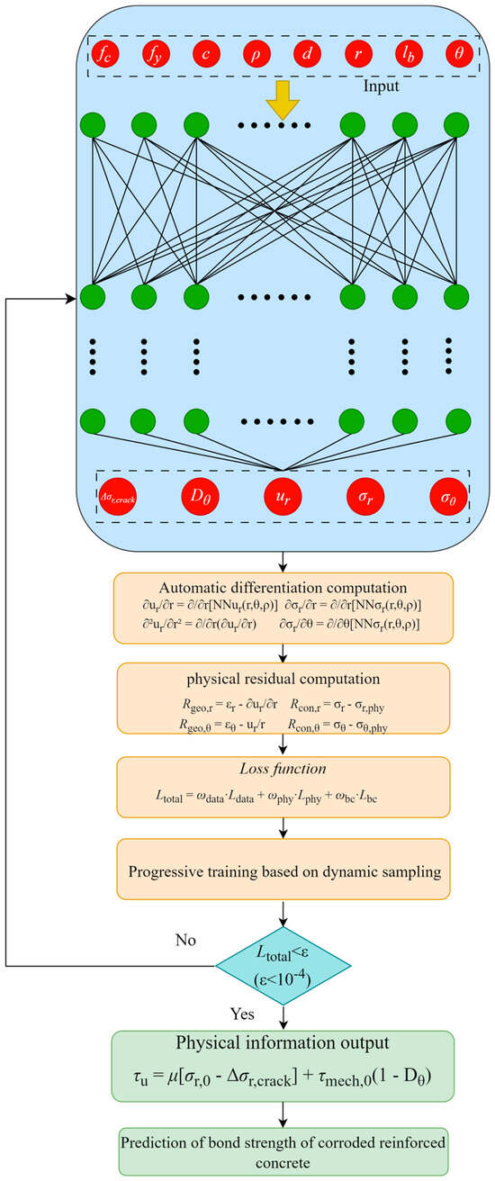
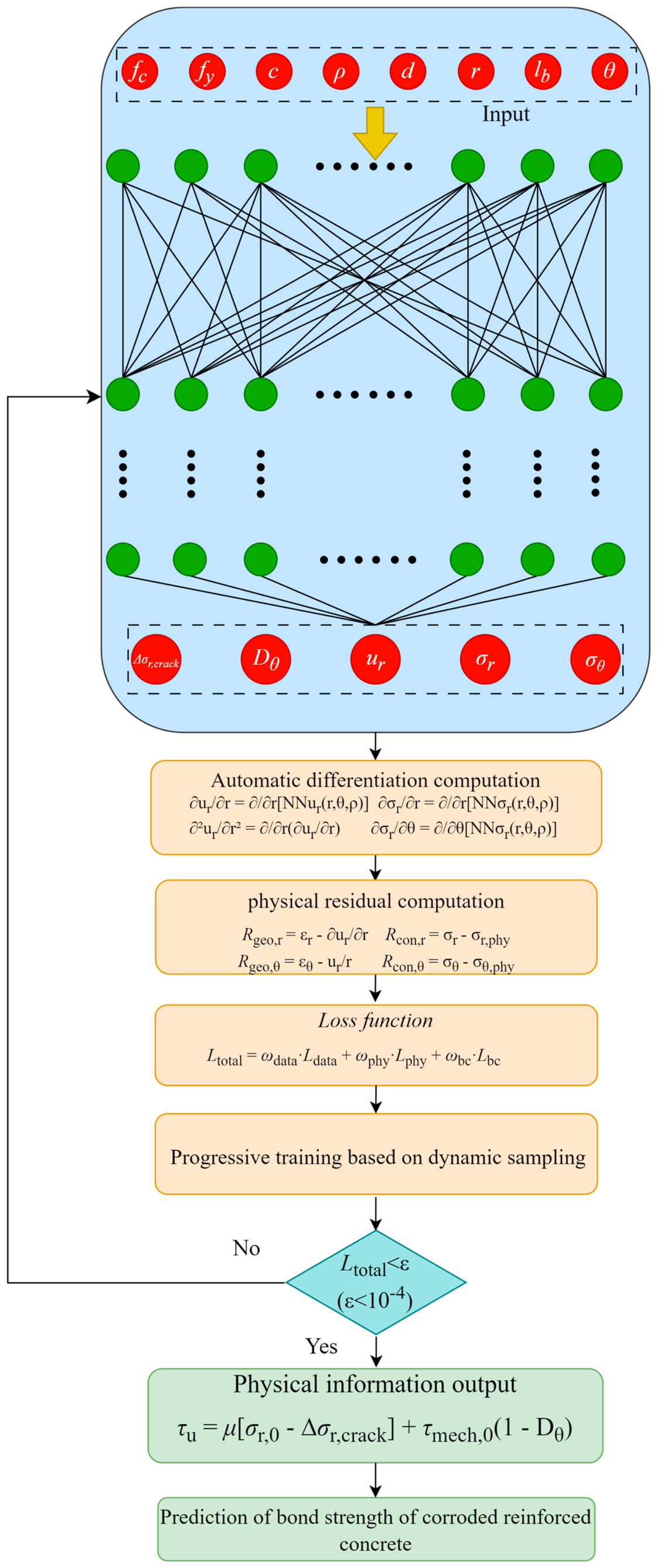
This study addresses these gaps through three key innovations. First, we construct a dedicated physical constraint framework based on the elastic thin-walled cylinder model, deriving differentiable relationships among rust expansion pressure, hoop stress, and radial displacement that are embedded at the loss-function level. Second, we account for the non-uniform filling of corrosion products and the stress redistribution after concrete cracking by introducing correction coefficients and empirical constitutive relationships. Third, the proposed framework maintains interpretability by embedding domain knowledge into the model architecture. Based on 598 sets of experimental data with some input variables (fc, d, lb, fy, ρ, c), we develop a mechanism–data dual-driven PINN model. The model’s performance is validated through comparison with conventional ML models (RF, XGBoost, SVM), existing empirical formulas, and accelerated corrosion experiments on RC specimens. The flowchart of the research program is shown in Figure 1.
Figure 1.
Flowchart of bond stress prediction.
2. Dataset Construction and Parameter Analysis
This study collected bond strength test data from 598 groups of corroded RC members [29,30,31,32,33,34]; the specific member parameters are shown in Table 1. Based on prior knowledge, six parameters that significantly influence corroded RC members were selected, covering geometric dimensions, material properties, reinforcement configuration, corrosion rate, and cover thickness: concrete axial compressive strength (fc), steel bar diameter (d), bond length (lb), steel yield strength (fy), corrosion rate (ρ), and cover thickness (c). The output variable is the reinforced concrete bond strength, ranging from 0.67 to 40.58 MPa.
Table 1.
Statistical values of various parameters.
In this study, the corrosion rate is defined as the cross-sectional loss rate, expressed in terms of both mass loss rate and steel bar cross-sectional loss rate:
where ρ is the loss rate of cross section; ΔA/ΔA0 is the loss rate of steel bars cross-sectional area; Δm/Δm0 is the loss rate of steel mass.
2.1. Categories and Distributions of Parameters
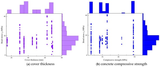
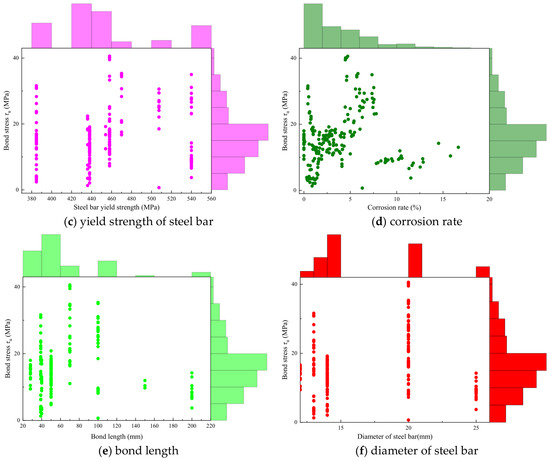
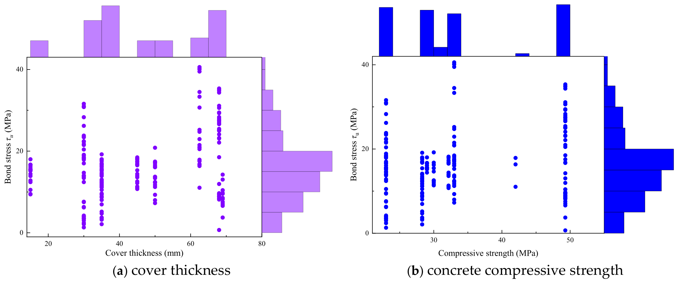
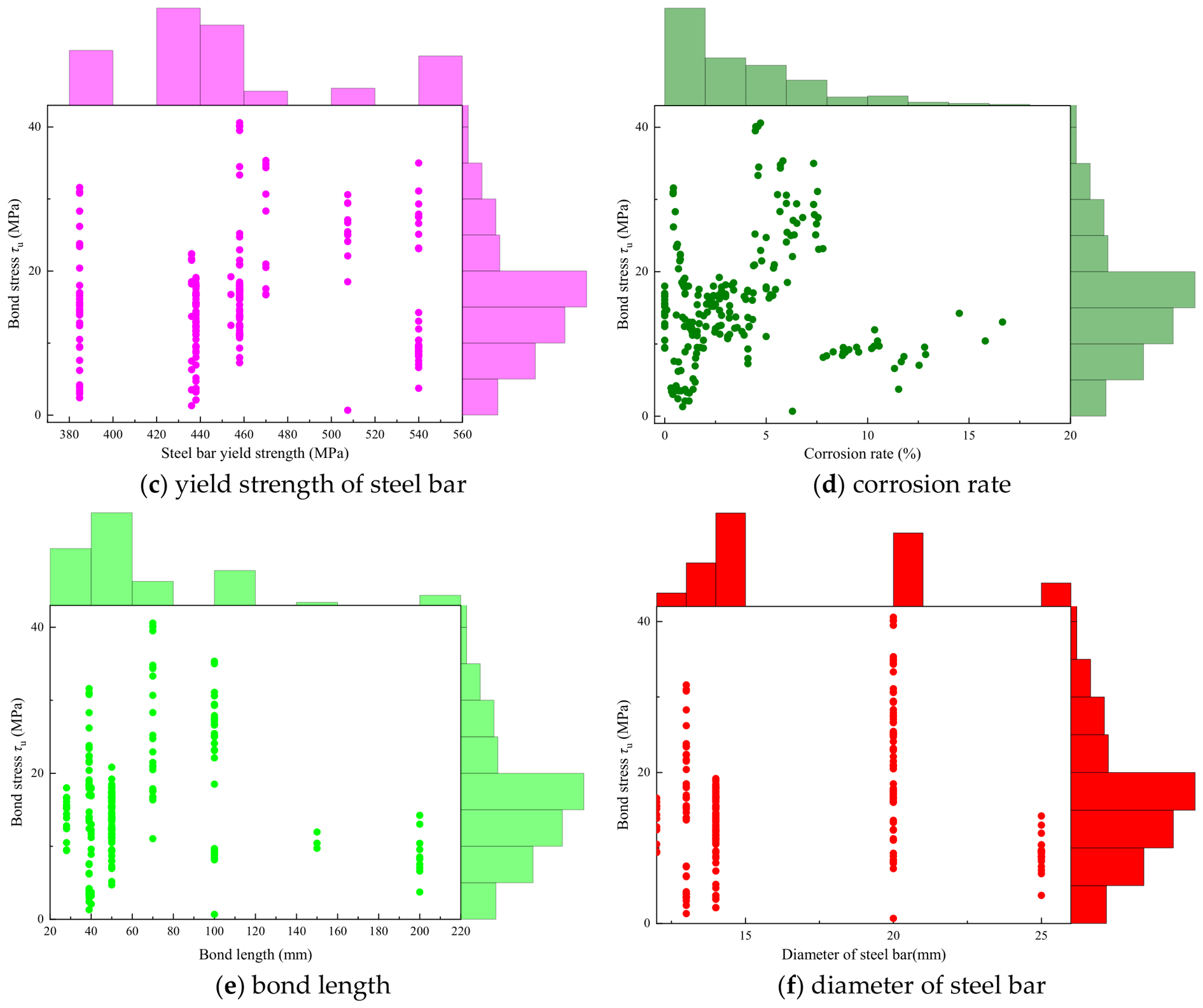
For corroded reinforced concrete specimens, the types and distributions of parameters affecting bond strength determine the evaluation accuracy of data-driven methods. Before applying ML methods, it is necessary to understand the categories and distributions of the input parameters and to assess their sensitivity to the prediction results. The classification and distribution of parameters affecting corroded RC components are shown in Figure 2, which indicates that the experimental dataset covers a wide range of each feature.
Figure 2.
Joint plot of features with target.
2.2. Parameter Correlation Analysis
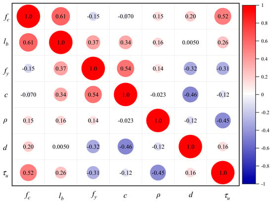
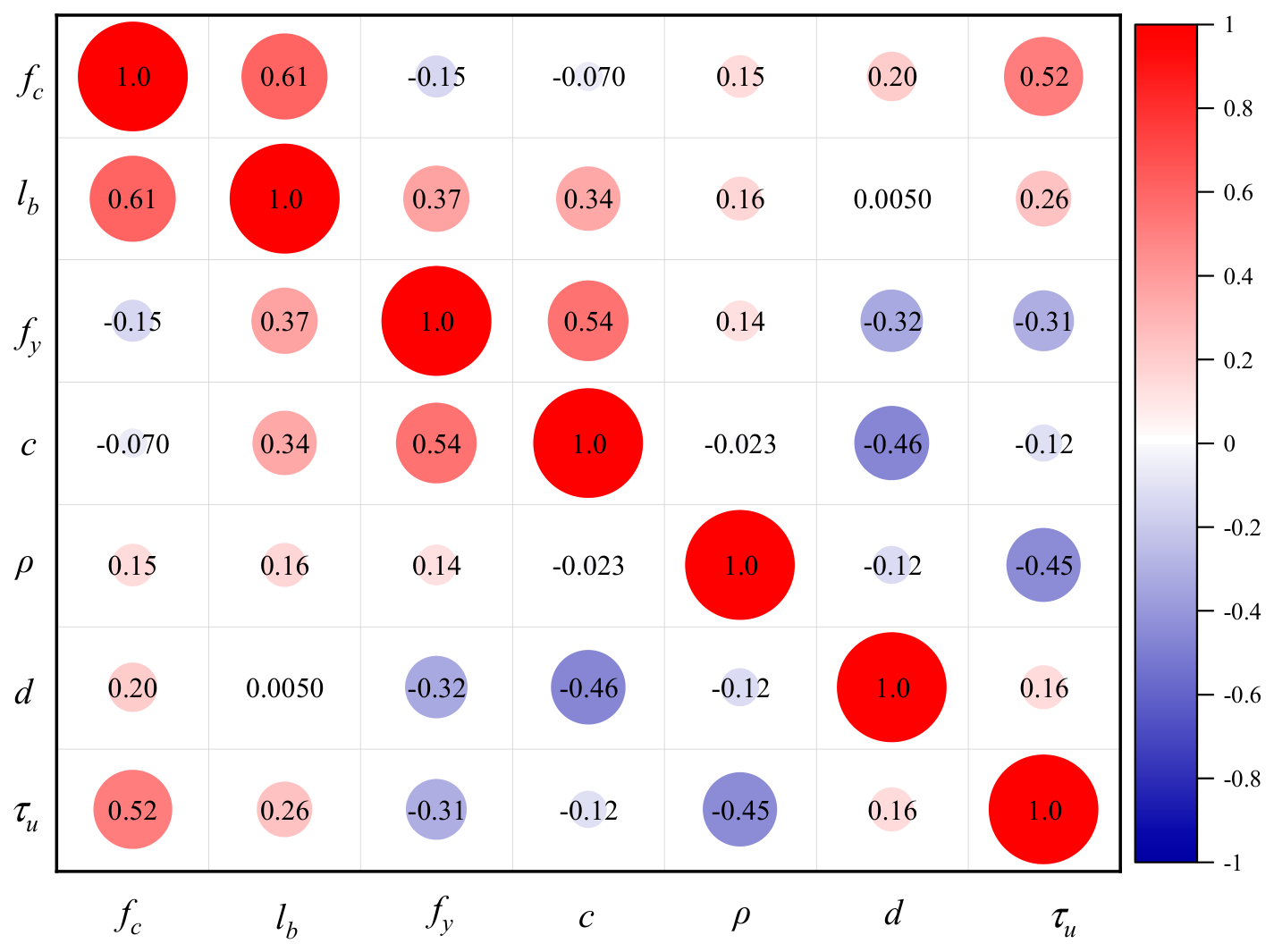
The distribution characteristics of the parameters guided further analysis of the collected database. The correlation between variables was studied using Equation (2), and the Pearson correlation coefficient matrix among all parameters is shown in Figure 3. To improve the effectiveness of the machine learning models, the correlation value between any two parameters should be kept below 0.8 to reduce the potential impact of multicollinearity. The parameter features selected in this study are therefore suitable for building machine learning models.
Figure 3.
Pearson correlation coefficient matrix.
2.3. Data Preprocessing and Dataset Partitioning
Before training, the raw experimental records were screened according to three criteria: (1) only specimens with complete records of bond strength, corrosion rate, concrete compressive strength, bar diameter, bond length, yield strength and cover thickness were retained; (2) specimens with obvious testing anomalies, inconsistent corrosion definitions, or incomplete parameter records were excluded; and (3) duplicate records were removed. The final database contains 598 groups. The dataset was randomly split into training, validation and test sets with proportions of 70%, 15% and 15%; the 10 mm-cover extrapolation subset (12 specimens) was held out separately and never used in training. Stratification was not applied because the database is dominated by low-to-moderate corrosion levels; to reduce the influence of the random split, the sensitivity of all models to the split was checked across five folds. Potential biases of the database should also be noted: cover thicknesses around 15–25 mm, concrete compressive strengths around 25–35 MPa and corrosion rates below 10% are over-represented, whereas corrosion rates above 15%, large bar diameters (>25 mm) and high-strength concrete are under-represented. These biases should be considered when extrapolating the results.
3. Model and Method
3.1. Mechanistic Sub-Model for the Corrosion Rate
The corrosion environment field determines the spatial and temporal distribution of the corrosion rate ρ (r, θ, t), which serves as an input to the PINN. This section establishes the governing equations, boundary conditions, initial conditions, and material parameters for the coupled diffusion–electrochemical problem.
3.1.1. Chloride Diffusion
Chloride ingress into concrete is governed by Fick’s second law:
where C is the chloride ion concentration of concrete; D(t) is the diffusion coefficient of chloride ions; x is the distance from the concrete surface; t is the diffusion time.
Boundary and initial conditions:
Under constant boundary conditions, Equation (3) admits the analytical solution:
where C0 is the initial chloride ion concentration in concrete; Cs is the concentration of chloride ions on the concrete surface; C(x, t) is the concentration of chloride ions at time t and erosion depth x; erf (•) is a function of error.
In this study, Equation (4) is used directly to compute the chloride concentration field, as the constant boundary condition assumption is valid for the accelerated corrosion tests considered. For general time-dependent boundary conditions, Equation (3) would be solved numerically via PINN.
Oxygen diffusion follows a similar formulation:
Boundary and initial conditions:
Under steady-state conditions (∂CO2/∂t ≈ 0, valid for long-term corrosion), Equation (5) admits a linear profile:
where DO2 is the diffusion coefficient of oxygen in concrete.
3.1.2. Electrochemical Reaction and Corrosion Rate
Corrosion initiation and propagation follow a three-step process governed by the concentration fields from Section 3.1.1.
Step 1: Depassivation condition. At each angular position θ on the steel surface, the protective oxide film breaks down when the chloride concentration reaches the threshold value Clim:
where x(θ) = c/cos(θ) is the diffusion path length at angle θ, and C(x,t) is given by Equation (4). Before tdepass, no corrosion occurs (ia = 0).
Step 2: Corrosion current density. After depassivation, the anodic current density ia(θ,t) is governed by the oxygen concentration at the steel surface C(O2) (θ, t), which is the rate-limiting factor for cathodic-controlled corrosion:
where i0,c is the reference cathodic exchange current density, CO2(θ, t) is the oxygen concentration at the steel surface from Equation (5a–e), and CO2ref is the reference oxygen concentration under saturated conditions.
For the accelerated corrosion tests in this study (constant current density applied externally), Equation (9) is replaced by the applied current density ia, applied = iapplied/A0, where iapplied is the constant impressed current and A0 is the steel surface area.
Step 3: Corrosion rate from Faraday’s law. The local cross-sectional loss ΔA (θ) is obtained by integrating ia (θ, t) over time:
The local corrosion rate at angle θ is as follows:
where M = 55.845 g/mol, z = 2, F = 96,485 C/mol, ρFe = 7870 kg/m3, and A0 is the initial cross-sectional area.
The corrosion medium diffusion model (Section 3.1) and the electrochemical model (Section 3.2) together characterize the corrosion environment that governs the temporal and spatial distribution of steel cross-section loss. Specifically, the chloride concentration C(x,t) from Equation (4) determines the time at which depassivation occurs at each point along the steel circumference, and the anodic current density ia from Equation (8) governs the local corrosion rate via Faraday’s law (Equation (9)). The resulting corrosion rate ρ = ΔAs/As0 serves as one of the input coordinates (r, θ, ρ, fc, lb, fy, c, d) to the PINN, characterizing the extent of material deterioration at each location on the steel surface. However, the corrosion rate alone does not capture the mechanical consequence of corrosion-namely, the rust expansion pressure and the resulting damage at the steel–concrete interface. This mechanical effect is addressed in Section 3.3 through a thin-walled cylinder model, which provides the physical governing equations (stress equilibrium, strain–displacement, and damage evolution) that are embedded as soft constraints in the PINN loss function. Section 3.3 then integrates both the corrosion environment inputs and the mechanical constraints into a unified PINN framework for bond strength prediction.
3.2. Rust Expansion Stress Model and Analytical Solution
The corrosion medium diffusion model (Section 3.1) determines the spatial and temporal distribution of the corrosion rate ρ(θ), which represents the local cross-sectional loss at each angular position on the steel surface. This section presents the analytical model that relates ρ(θ) to the rust expansion stress σr and hoop stress σθ, which serve as the physical constraints embedded in the PINN loss function.
3.2.1. Thin-Walled Cylinder Model
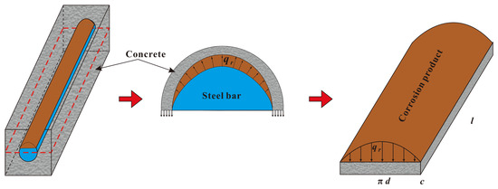
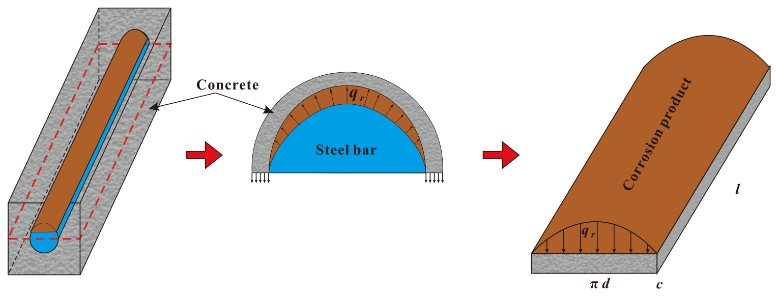
Determining the development of rust expansion stress is a prerequisite for accurately evaluating the bond strength of corroded reinforced concrete. To calculate the rust expansion stress at each point on the surface of the corroded steel bar, an elastic mechanics approach is adopted, modeling the corroded reinforced concrete as a thin-walled cylinder and expanding it into a concrete slab that resists the rust expansion force, as shown in Figure 4. The corrosion stress is calculated as follows:
where q0 is the corrosion stress; fct is the tensile strength of the concrete; d is the diameter of the corroded steel bar.
Figure 4.
Expansion model of the corroded reinforced concrete.
The concrete cover is modeled as a thin-walled cylinder of inner radius r0 = d/2 and outer radius r1 = d/2 + c. Where c is the cover thickness, the radial displacement ur satisfies the equilibrium equation in polar coordinates:
The boundary conditions are as follows:
where q0 is the rust expansion pressure at the interface.
3.2.2. Non-Uniform Corrosion
Due to the directional ingress of corrosive media (Section 3.1), the corrosion rate ρ varies along the steel bar circumference. Near the concrete cover side (θ = 0°), the corrosion rate reaches its maximum ρmax;
The angular distribution of the rust expansion pressure follows a parabolic decay:
where E is the elastic modulus of concrete, ν is Poisson’s ratio, and k = 2.2 is the rust expansion coefficient representing the volume ratio of corrosion products to the consumed steel. This value follows the experimental measurements by [35], which reported k ∈ [1.8, 2.5] for accelerated corrosion conditions.
The radial displacement at the inner boundary induced by corrosion expansion is as follows:
It should be noted that the thin-walled cylinder model assumes axisymmetric corrosion conditions, whereas in reality corrosion is often non-uniform due to the directional ingress of corrosive media. In this framework, the angular dependence of the corrosion rate ρ(θ) (derived from Section 3.1 and Section 3.2) is explicitly incorporated as an input to the PINN, allowing the model to capture non-axisymmetric effects. However, the analytical relationship between rust expansion pressure and hoop stress in Equations (11)–(13) remains derived under the axisymmetric assumption.
To make the mechanistic derivation explicit, the corrosion-induced mass loss is related to the cross-sectional loss by Δm = ρFe·ΔA·L, where ρFe = 7850 kg/m3 is the density of steel and L is the bar length over which corrosion is assumed to be uniformly distributed. If the volume expansion ratio of the corrosion products is n = Vrust/Vconsumed, the volume of corrosion products generated from the consumed steel is Vrust = n·ΔA·L. A part of this volume first fills the porous interfacial zone (Δpore); the remaining volume expansion resisted by the concrete cover is ΔVeff = (n − 1)·ΔA·L − Δpore. Under the thin-walled cylinder idealization, this effective expansion is converted into a uniform radial displacement ur = ΔVeff/(2πr0·L) at the steel-concrete interface, which, together with the boundary conditions in Equation (11b,c), yields the internal rust expansion pressure qb (= q0 in Equation (10)). The derivation assumes that: (1) the concrete cover behaves as a homogeneous, linear-elastic thin-walled cylinder; (2) corrosion products first fill the interfacial pores before significant pressure develops; (3) in the analytical solution the pressure is uniform around the circumference; and (4) cover cracking is represented indirectly through the damage variable Dθ and the angular pressure distribution in Equation (12). The uniform-pressure assumption is retained because the analytical model provides a differentiable, closed-form relationship between corrosion expansion and the resulting confinement stress; the non-uniform nature of corrosion is captured by the angularly dependent corrosion rate ρ(θ), the angular pressure distribution q0(θ), and the damage variable Dθ.
3.3. PINN Architecture, Physical Constraints and Loss Formulation for Bond-Strength Prediction
3.3.1. Network Architecture
The PINN structure designed in this paper is shown in Figure 5. The network input layer contains (r, θ, ρ, fc, lb, fy, c) neurons. The hidden layer adopts a 5-layer fully connected structure. To enforce physical consistency, the network outputs five intermediate physical variables: the radial displacement ur, the radial stress σr, the hoop stress σθ, the cracking-induced radial stress loss Δσr,crack, and the circumferential damage variable Dθ. The network architecture can be expressed as follows:
where Wi and bi are the weight matrix and bias vector of the i-th layer, respectively; Ψ is the nonlinear activation function; i is the number of hidden layers. The hyperbolic tangent (tanh) function is selected as the activation function due to its continuous and smooth second-order derivative characteristics, which are essential for solving higher-order partial differential equations in the stress field. The specific expression is as follows:
Figure 5.
Flow chart of the PINN model for predicting bond strength of corroded reinforced concrete.
The output layer employs a linear activation function to allow unrestricted output of physical quantities. The final bond strength τu is then computed through a physics-informed output layer as follows:
where μ is the friction coefficient, σr,0 is the initial radial compressive stress, and τmech,0 is the initial mechanical bond strength.
Where μ is the friction coefficient, which is a trainable parameter bounded between 0 and 1 and physically represents the interfacial friction between the corroded bar and the surrounding concrete; σr,0 is the initial radial compressive stress at the interface before corrosion-induced damage; and τmech,0 is the initial mechanical bond strength provided by the rib-interlock mechanism of an uncorroded deformed bar. In the present implementation, μ and τmech,0 are learned by the network as trainable scalar parameters, with μ initialized at 0.5 and τmech,0 initialized from the estimated bond strength of the uncorroded bar; both are constrained to physically admissible ranges. This friction-plus-mechanical-interlock decomposition follows the classical bond mechanism [6,15,36], in which corrosion initially increases the frictional contribution through rust expansion pressure and subsequently degrades both components.
3.3.2. Physical Constraints Embedded via Automatic Differentiation
The physical consistency of the neural network is enforced by embedding the governing equations of corroded reinforced concrete into the loss function. Through automatic differentiation (AD), the partial derivatives of the network outputs with respect to all independent input coordinates (r, θ, ρ, fc, lb, fy, c) are computed by the chain rule, ensuring computational accuracy and optimization efficiency. A single multi-output neural network is used: all five physical fields (ur, σr, σθ, Δσr, crack, Dθ) share the same hidden layers and are produced by separate output neurons. Coupling between the fields is enforced both by this shared representation and by the physical constraints in Equations (23)–(27), so separate networks with ad hoc coupling terms are not required. Let x = (r, θ, ρ, fc, lb, fy, c, d) denote the input vector and u = (ur, σr, σθ, Δσr, crack, Dθ) the outputs of the single multi-output network. The automatic differentiation formulations applicable to the radial and circumferential coordinates are:
where ωj is the weight vector corresponding to the j-th output neuron in the output layer; D is the diagonal matrix obtained by deriving the activation function tanh; W is the weight matrix for each layer of the network; ei is the i-th standard unit basis vector.
The strain-displacement relationships are as follows:
where εr and εθ are the radial and hoop strains, respectively.
The constitutive equations can be expressed as follows:
where σr is the radial stress; σθ is the hoop stress at the steel-concrete interface; σθ,max is the maximum hoop stress attained before cracking; fα is the critical hoop tensile stress threshold adopted for damage initiation, which is taken equal to the concrete tensile strength fct (fα = fct) rather than a free fitting parameter; and Dθ is the circumferential damage variable, which evolves from 0 (undamaged) to 1 (complete loss of confinement). The damage criterion Dθ = 0.1 at the onset of microcrack coalescence follows the micromechanics-based damage model of Jiang et al. [35], and this threshold is consistent with the present experimental results, in which visible cover cracking initiates at corrosion rates of approximately 4% (Section 5.3).
The equilibrium equation in polar coordinates is as follows:
where r is the radial coordinate.
3.3.3. Boundary Conditions
The boundary conditions imposed on the PINN model are as follows:
At the steel-concrete interface (r = d/2, where d is the diameter of the corroded steel bar):
At the outer edge of the cover layer (r = d/2 +c, where c is the thickness of the concrete cover):
Periodicity conditions in the circumferential direction:
3.3.4. Loss Function Construction
Model performance is evaluated by constructing a composite loss function that reduces the deviation between the network’s predictions and the actual values while enforcing physical consistency. By iteratively optimizing the network parameters to minimize the loss function, the governing equations are progressively solved, with the decrease in loss value directly reflecting the improvement in prediction accuracy. The loss function of the PINN model is as follows:
where ωdata, ωphy, and ωbc are the weights of data loss, physical loss, and boundary loss, respectively.
The data loss term quantifies the discrepancy between predicted and true bond strengths:
The physical loss term incorporates the residuals of the governing equations:
where the residuals are defined as follows:
The boundary loss term enforces the boundary conditions:
where the residuals are defined as follows:
The λi weight parameter adopts an adaptive dynamic adjustment and loss balancing strategy, and λi is updated every 100 rounds according to the residual ratio.
3.3.5. Training Strategy
To ensure the stability and physical consistency of the prediction results from the proposed model, the training process is divided into four stages. Stage 1: Data loss minimization is adopted as the primary objective, enabling the prediction results to rapidly approach the true observed values and establishing an initial mapping relationship. Stage 2: An adaptive method is employed to adjust the weight of the physical loss, gradually introducing physical constraints in a progressive manner to avoid training instability caused by abrupt changes in the physical loss term. Stage 3: A complete composite loss function is adopted, simultaneously activating the data loss, physical loss, and boundary loss to achieve multi-objective joint optimization. Stage 4: The learning rate is gradually reduced, and the grid parameters are fine-tuned to further improve the prediction accuracy. The PINN was implemented in Python using PyTorch 2.0.1 [36] for automatic differentiation and network training, NumPy 1.16.0 [37] and SciPy 1.2.1 [38] were used for data processing and numerical routines.
The loss weights were determined through preliminary sensitivity analysis. The physical loss weight λ1 was scanned over [0.01, 0.1, 0.5, 1.0, 5.0, 10.0] with λ2 = 1.0 fixed. The optimal range was found to be λ1 ∈ [0.5, 1.0], where Ldata and Lphy achieved balanced convergence without one dominating the other. Outside this range (λ1 < 0.1), physical constraints were insufficient, leading to physically inconsistent predictions; at λ1 > 5.0, data fitting degraded significantly. In the final training, λ1 was initialized at 0.01 (Stage 1), linearly increased to 1.0 over epochs 500–2000 (Stage 2), and held constant through Stages 3–4. The boundary loss weight λ2 was fixed at 1.0 throughout all stages, as the boundary residuals were of comparable magnitude to the data loss. A complementary sensitivity analysis was performed for the Stage-2 transition window and the number of collocation points. Transition windows of [200, 500, 1000, 2000] epochs and collocation-point counts of [100, 300, 500, 1000] per epoch were tested. Training remained stable for windows of 500–2000 epochs; 500 collocation points per epoch provided the best trade-off between physical-constraint satisfaction and computational cost, whereas 100 points led to larger physics residuals and 1000 points gave no further reduction in validation error. The chosen values (transition over 500–2000 epochs and 500 points per epoch) were therefore adopted.
The Adam optimizer is adopted with an initial learning rate of 1 × 10⁻³, which decays by a factor of 0.9 every 2000 epochs. An early stopping mechanism terminates training when the validation loss shows no decrease for 50 consecutive epochs. A dynamic sampling strategy is implemented, where 500 new residual points are added at each epoch within the computational domain [d/2, d/2 + c] × [0, 2π] using Latin hypercube sampling, ensuring comprehensive coverage of the spatial domain.
4. Results and Discussions
4.1. Chloride Ion Concentration on the Surface of Steel Bars
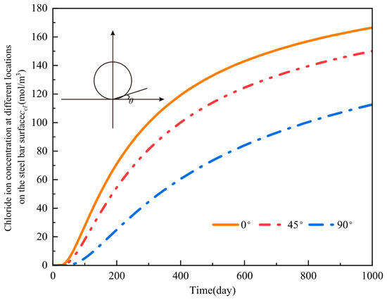
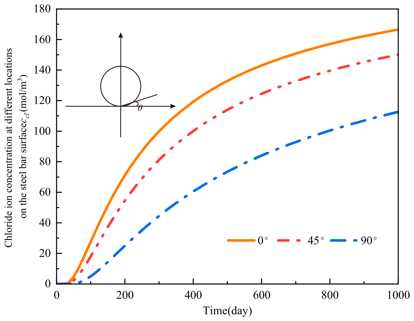
During the service life of a reinforced concrete structure, corrosive media (chloride ions, oxygen, water) diffuse from the concrete surface inward, driven by a concentration gradient. Figure 6 shows the concentration distribution of chloride ions and oxygen at different positions on the steel surface. As shown in the figure, the concentration of corrosive media gradually increases with service life. The angle shown in Figure 6 represents the angle between the observation point and the reinforcement surface point nearest to the concrete cover. Further observation reveals a large difference in concentration at different positions, because the 0° point is closest to the concrete surface. The corrosive medium first reaches this point and gradually accumulates. After the chloride ion concentration reaches the threshold, the oxide film on the steel surface is destroyed, and the electrochemical reaction begins.
Figure 6.
Concentration distribution of corrosive medium in circumferential direction of reinforcement.
4.2. Current Density at Steel-Concrete Interface
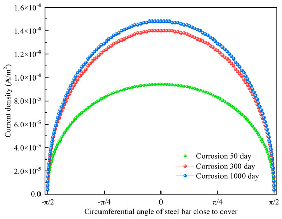
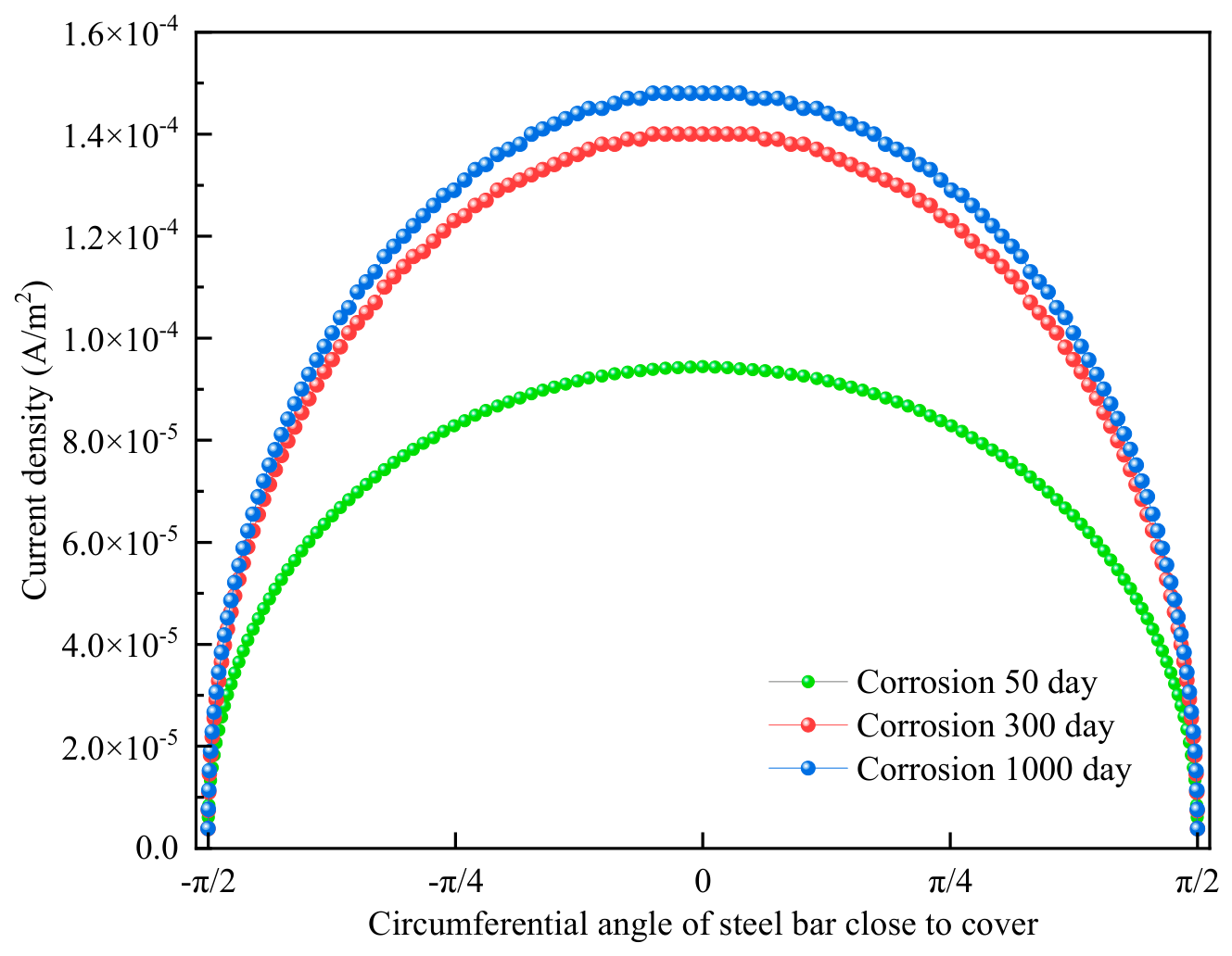
As corrosive media continuously accumulate at the steel–concrete interface, their concentration gradually increases. The oxide film on the steel bar surface near the concrete cover is destroyed, forming an activated area, while the steel bar on the side farther from the cover remains in an inactive area. Electrochemical reactions occur immediately. In the activated area, iron atoms lose electrons and undergo oxidation; in the inactive area, oxygen and water gain electrons and undergo reduction, generating a corrosion current. The current density is controlled by the concentration of the corrosive medium. Since the concentration of the corrosive medium is non-uniformly distributed on the steel bar surface, the corrosion current density at each point in the circumferential direction also varies. As shown in Figure 7, the maximum current density occurs at the 0° point and gradually decreases along the circumference, consistent with the concentration distribution of the corrosive medium. Further observation shows that as the service life increases, the current density at each point around the steel bar also increases.
Figure 7.
Current density distribution in the circumferential direction of reinforcement.
4.3. Validation of PINN-Predicted Rust Expansion Stress
A key advantage of the PINN framework is its ability to predict intermediate physical quantities, the rust expansion stress σr and hoop stress σθ-alongside the final bond strength τu. These intermediate predictions can be validated against the analytical thin-walled cylinder model (Section 3.3) to verify that the physical constraints are correctly learned.
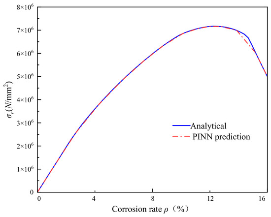
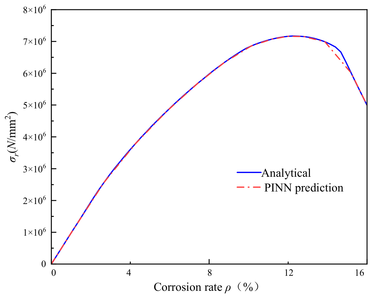
Figure 8 compares the radial stress σr predicted by the PINN at the steel-concrete interface (r = d/2) with the analytical solution from Equation (12) for corrosion rates ranging from 0% to 16%. The PINN predictions follow the analytical curve closely, with a mean relative error of 2.3%, confirming that the equilibrium equation (Equation (27)) and boundary conditions (Equations (29) and (30)) are effectively enforced through the physics-informed loss terms.
Figure 8.
Comparison of PINN-predicted radial stress with the analytical result.
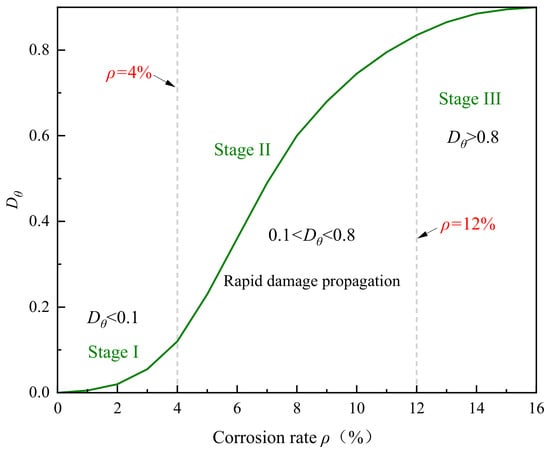
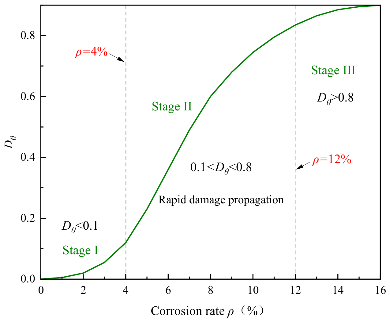
Figure 9 shows the evolution of the circumferential damage variable Dθ with corrosion rate. Below ρ ≈ 4%, Dθ remains near 0.1, indicating that the concrete cover has not yet cracked, which is consistent with the well-known observation that corrosion products first fill the porous interfacial zone before generating significant expansive pressure. In the range ρ = 4–12%, Dθ increases sharply, corresponding to the initiation and propagation of cover cracking. Beyond ρ = 12%, Dθ approaches 1.0, signifying complete loss of confinement. This piecewise behavior is not explicitly programmed into the network but emerges naturally from the embedded damage constitutive relationship (Equations (25) and (26)), demonstrating that the PINN captures the correct physics without being told the exact cracking threshold. The damage threshold Dθ < 0.1 for the uncracked state and Dθ → 1.0 for complete confinement loss are defined based on the micromechanics-based damage model proposed by [39], in which Dθ = 0.1 corresponds to the onset of microcrack coalescence at the steel–concrete interface. It should be noted that this damage variable represents corrosion-induced degradation of the confining mechanism only; bond degradation due to cyclic loading or other mechanical actions is beyond the scope of this study.
Figure 9.
Development of circumferential damage variable Dθ with corrosion rate.
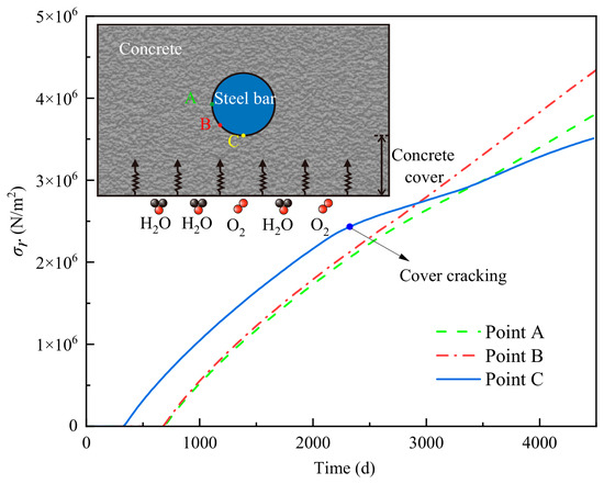
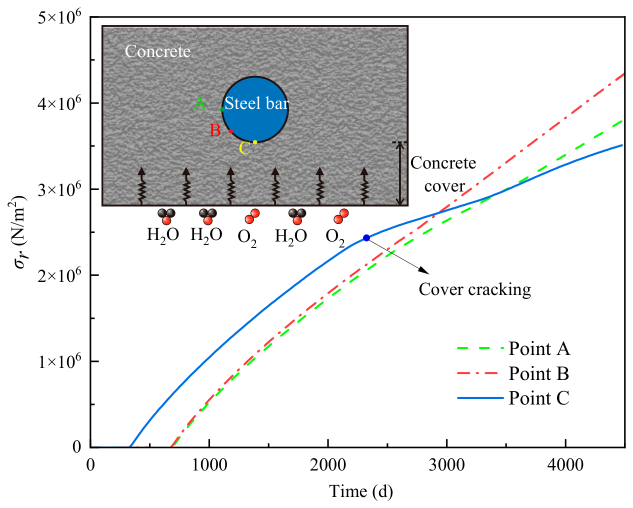
Figure 10 plots the PINN-predicted rust expansion stress against the corrosion duration for three angular positions (θ = 0°, 45°, and 90°). At θ = 0° (nearest to the concrete surface), the stress develops fastest and reaches the cracking threshold earliest, consistent with the concentration and current density results from Section 4.1 and Section 4.2. At θ = 90°, the stress develops more slowly due to the longer diffusion path, highlighting the non-uniform nature of corrosion-induced damage.
Figure 10.
Corrosion expansion stress development.
4.4. Relationship Between Hoop Stress Degradation and Bond Strength Loss
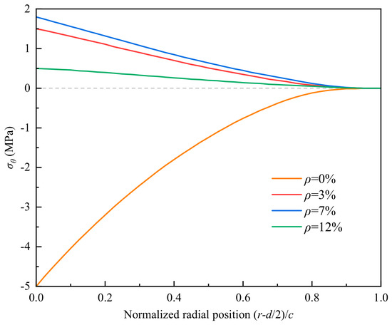
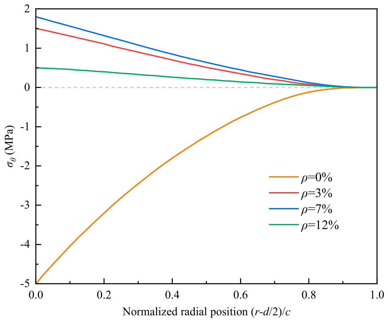
While Section 4.3 focuses on the radial stress at the interface, the hoop stress σθ governs the confinement that enables frictional resistance and mechanical interlock. Figure 11 shows the PINN-predicted hoop stress distribution along the radial direction at the 0° position for four corrosion levels (ρ = 0%, 3%, 7%, 14%).
Figure 11.
Radial distribution of circumferential stress under different corrosion rates.
For the uncorroded case (ρ = 0%), the hoop stress is compressive throughout the cover thickness, providing full confinement. As corrosion progresses (ρ = 3%), the hoop stress near the interface becomes tensile due to rust expansion, reducing the effective confinement available for bond resistance. At ρ = 7% (near the cracking threshold for the 0° position), the tensile hoop stress exceeds the concrete tensile strength fct, and the damage variable Dθ rises sharply, as shown in Figure 9. Beyond ρ = 12%, the hoop stress decreases significantly because cracked concrete can no longer sustain tensile stress, and the confinement mechanism is essentially lost.
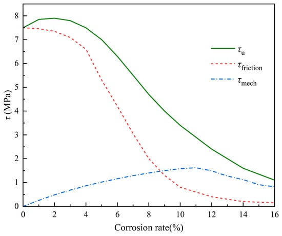
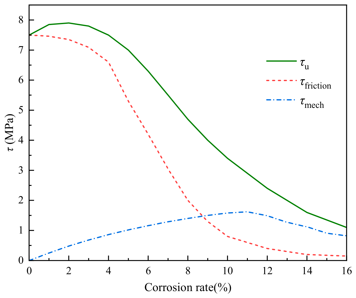
Figure 12 decomposes the bond strength τu into its two components per Equation (19): the frictional component μ·σr and the mechanical interlock component τmech. At low corrosion rates (ρ < 3%), the frictional component actually increases slightly due to rust expansion pressure-the same “first increase” phenomenon noted in Section 5.1 for the total bond strength. This confirms that the PINN correctly captures the competing effects of corrosion: initial confinement enhancement followed by cover cracking and strength degradation. At high corrosion rates (ρ > 10%), both components decay significantly, but the mechanical interlock component decays faster, indicating that the dominant failure mode shifts from friction loss to rib-bearing degradation as corrosion progresses. This faster decay of the mechanical interlock component is consistent with experimental observations that corrosion preferentially damages the rib-bearing mechanism, while the frictional contribution persists as long as residual confinement remains [6,15,36].
Figure 12.
Bond strength is decomposed into a friction component and a mechanical bite component.
The decomposition in Figure 12 is a unique capability of the PINN framework: purely data-driven models (XGBoost, RF, SVM) can only predict the total bond strength, whereas the physics-informed architecture enables access to intermediate mechanical quantities that provide mechanistic insight into the failure process.
4.5. Physics Loss Residual Analysis
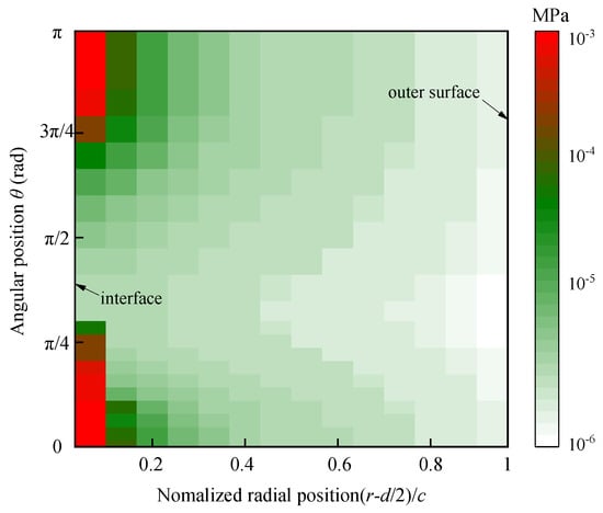
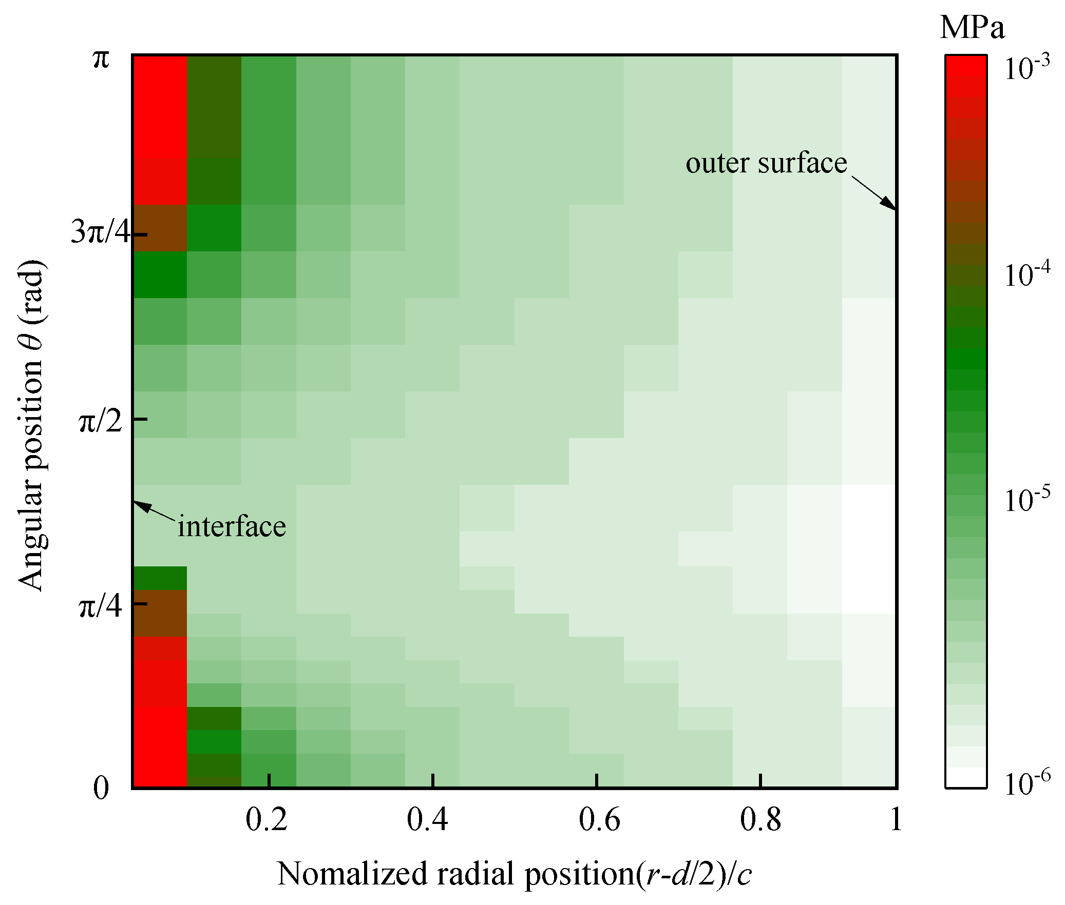
To verify that the PINN has effectively learned the embedded physical constraints, Figure 13 presents the residuals of the three governing equations (Equations (38)–(40)) over the computational domain after training.
Figure 13.
Spatial distribution of the equilibrium equation residual.
Figure 13 shows the spatial distribution of the equilibrium equation residual f1 = ∂σr/∂r + (σr − σθ)/r across the domain [d/2, d/2 + c] × [0, 2π]. The residual values are on the order of 10−3–10−2 MPa, which is three to four orders of magnitude smaller than the stress values themselves, indicating that the equilibrium condition is satisfied to high precision. The largest residuals occur near the steel–concrete interface (r = d/2) at θ = 0°, where the stress gradients are steepest-a pattern consistent with the known challenge of PINNs near boundary layers.
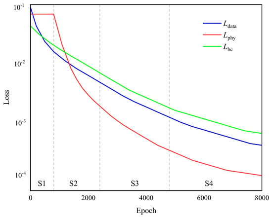
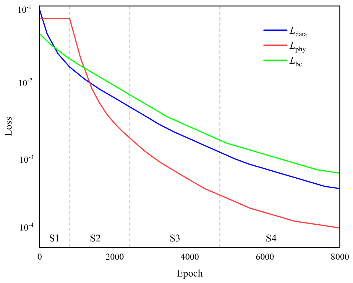
Figure 14 tracks the evolution of the three loss components (Ldata, Lphy, Lbc) during the four-stage training process described in Section 3.3.5). In Stage 1, Ldata decreases rapidly as the network learns the basic input–output mapping. In Stage 2 (500–2000 epochs), the physical loss weight ωphy is gradually increased, and Lphy begins to decrease while Ldata remains stable. In Stage 3 (2000–4000 epochs), all three losses are jointly minimized, with Lphy reaching its final value of 1.8 × 10⁻³. Stage 4 (4000–8000 epochs) fine-tunes the parameters with a reduced learning rate, reducing Ldata by an additional 12% without degrading Lphy or Lbc. The smooth convergence trajectory and the final loss magnitudes confirm that the multi-objective optimization strategy is effective and that no conflict between data fitting and physical consistency arises.
Figure 14.
Evolution of loss components during the four−stage training process.
These residual results provide direct evidence that the PINN framework achieves the intended physics–data integration: the network not only fits the experimental bond strength data but also satisfies the underlying governing equations to within acceptable tolerances.
5. Model Validation
5.1. Comparison of Different ML Prediction Models
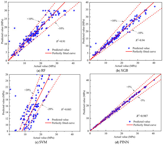
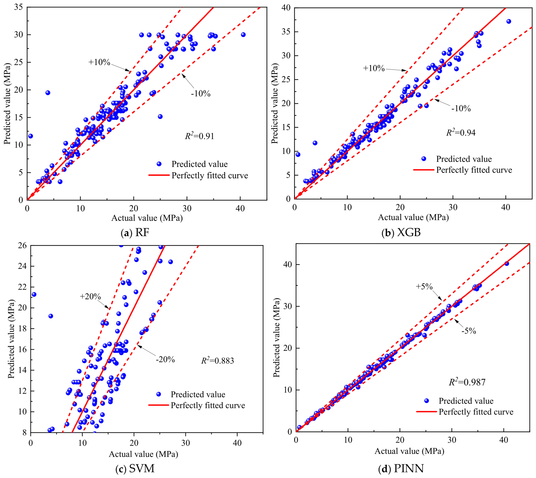
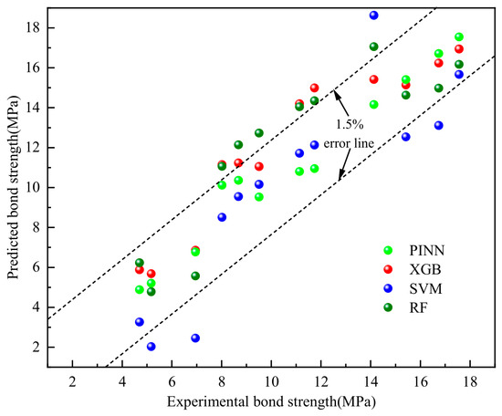
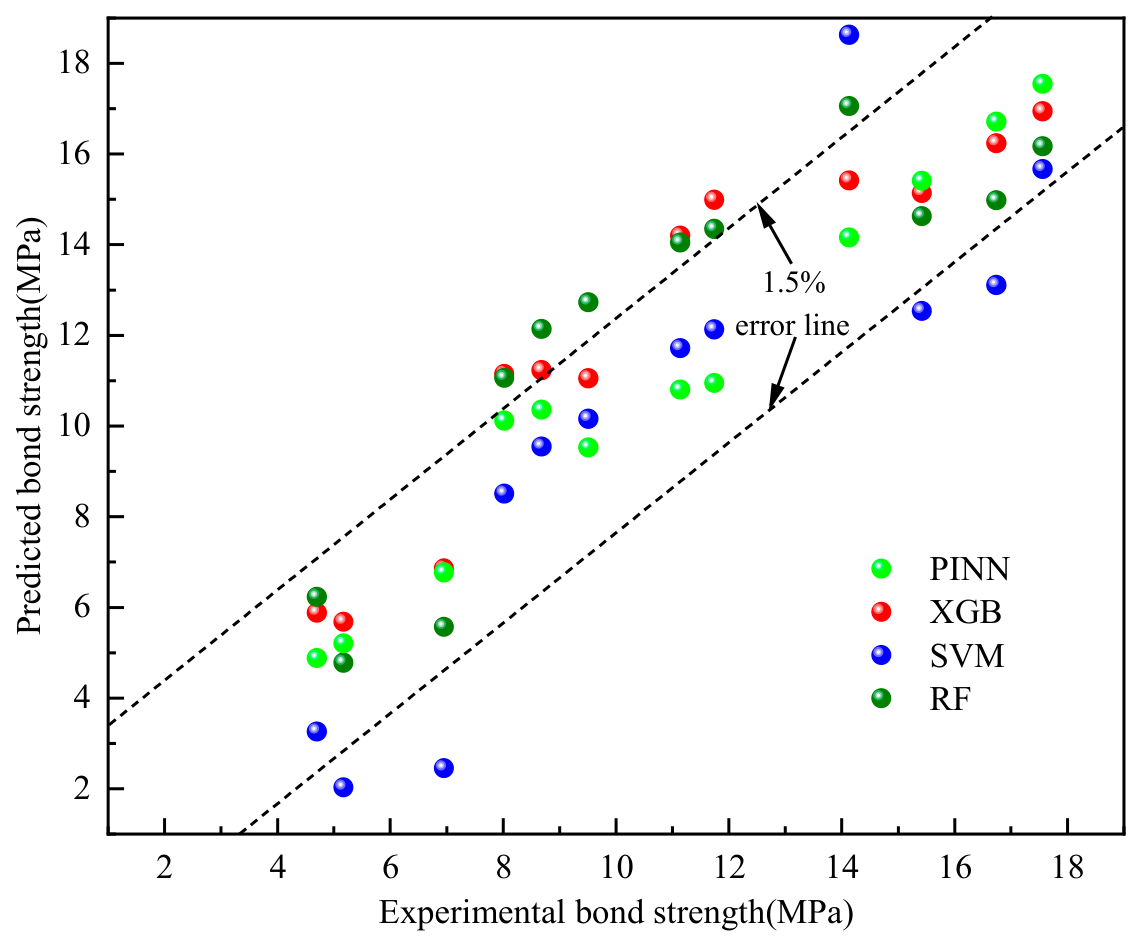
The prediction results of each ML model are shown in Figure 15. The results indicate that PINN achieves the best predictive performance, with all evaluation metrics superior to those of the other models. To systematically evaluate the extrapolation capability of the PINN model beyond the range of the training data, the cover thickness in the existing training dataset range from 15 mm to 69 mm. To test the model’s extrapolation performance, components with a cover of 10 mm were selected as the extrapolation test set (12 independent samples in total). The models compared include PINN, XGBoost, RF, and SVM. Figure 16 shows the predictions of bond strength for components with a 10 mm cover under different corrosion rates by each model. As can be seen from Figure 16, the PINN model demonstrates excellent prediction accuracy and physical consistency in the diameter extrapolation scenario (15 mm → 10 mm), with the prediction error controlled within 1.5%, significantly outperforming models such as XGBoost, SVM, and RF.
Figure 15.
Prediction of different ML Models.
Figure 16.
Comparison of extrapolation capabilities of different models.
All data-driven baseline models were tuned before comparison. A five-fold cross-validated randomized/grid search was used to optimize the hyperparameters of XGBoost, RF and SVM. For XGBoost, the number of estimators, maximum depth, learning rate and subsample ratio were searched; for RF, the number of estimators, maximum depth, minimum samples per split and maximum features were searched; for SVM, the kernel type, regularization parameter C and kernel coefficient γ were searched. The final settings were selected according to the lowest validation SMAPE, and identical training/validation/test splits were used for all models. The reported metrics are the mean values over the five folds; the corresponding standard deviations were small (R2 standard deviations below 0.02 for all models). A Wilcoxon signed-rank test further confirmed that the improvements of the PINN over XGBoost, RF and SVM are statistically significant (p < 0.05).
5.2. Comparison with Prior Mathematical Models
A comparative analysis was conducted between the proposed PINN model and established mathematical models from the literature to verify its applicability [37,38,39]. The fitting formula of the mathematical model is shown in Formulae (41)–(43):
Jiang’s [40] model is as follows:
where ρ is the corrosion rate of the steel bar; τu is the ultimate bond strength; Kst is the confinement effect of stirrups; Kco is the confinement effect of concrete; k1 is 0.514.
Feng’s [41] model is as follows:
where ρ is the corrosion rate of the steel bar; d is the diameter of the steel bar; c is the thickness of the concrete cover.
Bhargava’s [42] model is as follows:
where τu (0) is the bond strength between steel bar and concrete for uncorroded specimens.
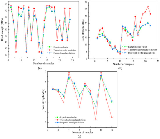
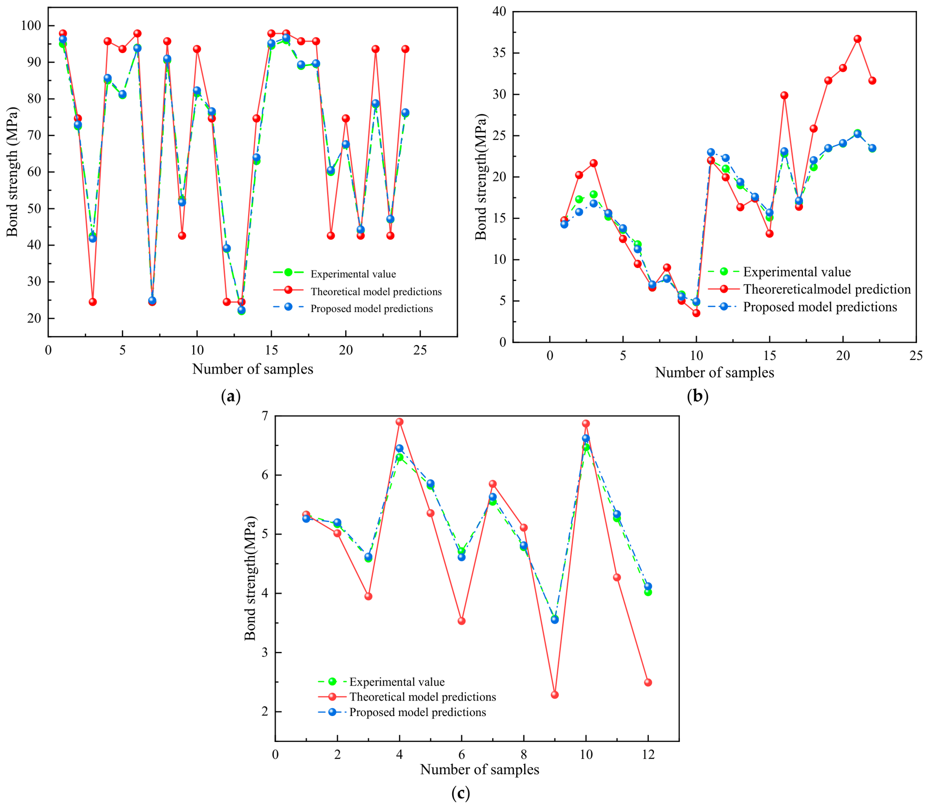
The prediction results of the mathematical models and the proposed model are shown in Figure 17. As shown in Figure 17a–c, the predictions of the proposed method are consistent with the actual values and follow the same trends as the existing models. To further evaluate prediction accuracy, performance evaluation of the proposed model and existing models was carried out, and the relevant evaluation metrics are shown in the table. In summary, compared with established mathematical models, the proposed approach exhibits higher accuracy in predicting the bond strength of corroded steel-reinforced concrete and is broadly applicable.
Figure 17.
Comparison between proposed model and theoretical model. (a) Comparison with the model in [36]. (b) Comparison with model in [37]. (c) Comparison with the model in [38].
5.3. Test Verification
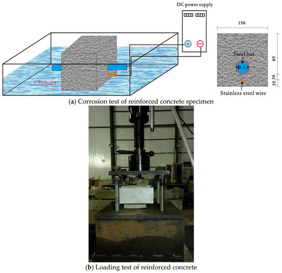
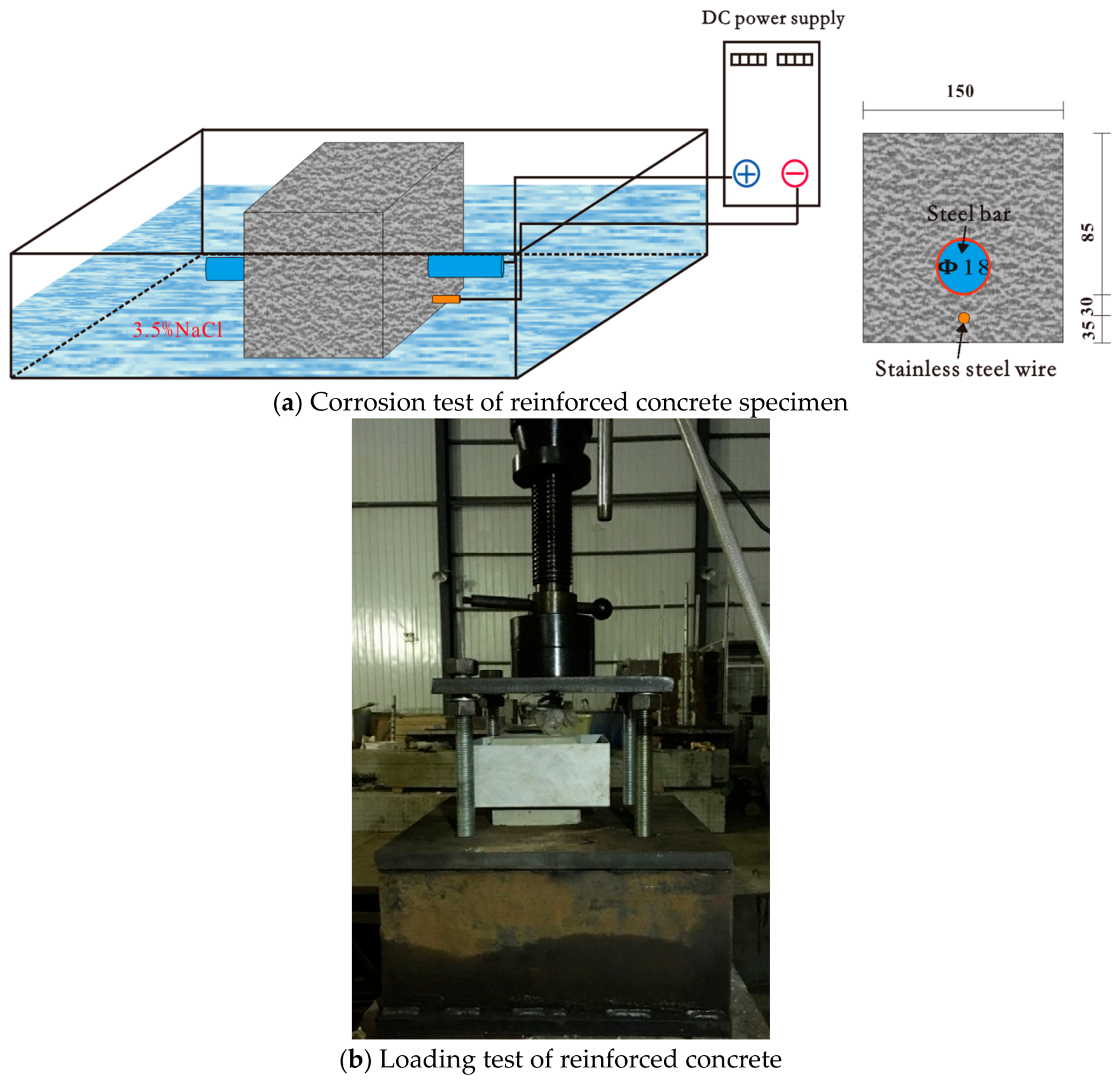
To investigate the applicability of PINN, accelerated corrosion tests and bond strength tests were conducted on reinforced concrete specimens. The concrete specimens were cubes with a side length of 150 mm, each containing a deformed steel bar of 18 mm in diameter, with a concrete cover thickness of 30 mm, as shown in Figure 18. The concrete compressive strength was 35 MPa, and the yield strength and ultimate strength of the steel bar were 473.3 MPa and 604.5 MPa, respectively. To simulate realistic corrosion conditions, the built-in auxiliary electrode method was adopted for accelerated corrosion testing. Stainless steel wires with a small cross-section were pre-placed in the concrete cover layer near the steel bar as auxiliary electrodes. After curing, the specimens were immersed in a 3.5% NaCl solution for three days and then connected to a stabilized DC power supply to initiate accelerated corrosion. The liquid level was controlled to fully submerge the steel bar, with the bar connected to the anode and the stainless steel wire connected to the cathode. A constant-current method was used to control the corrosion rate, yielding two specimens for each target corrosion rate of 2%, 4%, 8%, and 15%. The experimental and predicted bond strengths of the RC specimens are shown in Table 2.
Figure 18.
Devices used for accelerated corrosion and loading test (unit: mm).
Table 2.
Experimental and predicted bond strength of RC specimens.
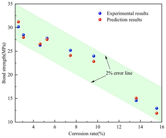
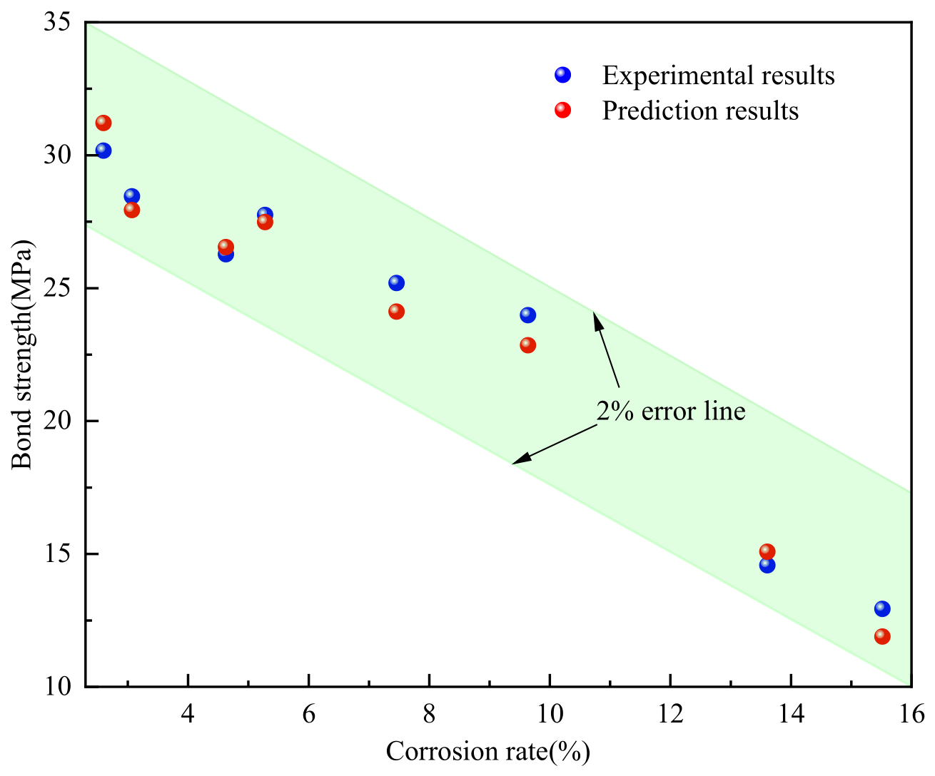
The predictions obtained using the PINN method were compared with the experimental results. As shown in Figure 19, at low corrosion rates, the bond strengths predicted by the PINN model agreed well with the experimental values. For specimen RC-4-1 (corrosion rate of 4.63%), the experimentally measured bond strength was 26.27 MPa, while the PINN-predicted value was 26.54 MPa, with a relative error of only 1.02%. For specimen RC-8-1 (corrosion rate of 9.64%), the experimental and predicted values were 23.98 MPa and 23.55 MPa, respectively, with a relative error of 1.8%. When the corrosion rate increased to 15.52% (specimen RC-14-2), the experimental bond strength decreased to 12.93 MPa, and the predicted value was 12.66 MPa, with an error of 2%. Overall, the prediction errors for all specimens were within 2%, with an average relative error of 1.66% and a standard deviation of 0.42%, indicating that the PINN method achieves high prediction accuracy.
Figure 19.
Comparison of prediction results and experimental results.
Further observation reveals that the PINN not only accurately captures the overall decreasing trend of bond strength with increasing corrosion rate but also effectively reflects the nonlinear degradation characteristics observed in the experiments. At low corrosion rates (<4%), the bond strength decreases relatively gently, and both PINN predictions and experimental results exhibit an approximately linear relationship. In the medium-to-high corrosion rate range (>8%), the bond strength declines more rapidly, and the experimental data show pronounced nonlinear decay. By incorporating physical governing equations (such as damage evolution and bond-slip constitutive relationships), the PINN model successfully fits this trend. Moreover, when the corrosion rate approaches 14%, some experimental points exhibit considerable scatter (standard deviation of 0.23 MPa); nevertheless, the PINN predictions remain within the 98% confidence interval of the experimental data, demonstrating the model’s good generalization capability.
6. Conclusions
In this study, a prediction model incorporating the development of rust expansion stress was established using the PINN algorithm. Based on the analysis presented, the following conclusions are drawn:
- (1)
- By modeling the concrete cover as an expanding plate based on elastic thin-walled cylinder theory, the corrosion expansion stress was analytically derived and embedded as a differentiable physical constraint in the PINN loss function. This enables the network to learn mechanically consistent representations even under limited training data.
- (2)
- The proposed PINN model outperforms conventional ML models (XGBoost, RF, SVM) and existing empirical formulas across all evaluation metrics. Compared to XGBoost, RF, and SVM, the proposed model improves R2 by 9.97%, 15.66%, and 5.49%, and reduces SMAPE by 45.56%, 58.87%, and 33.91%, respectively. These improvements are attributed to the effective guidance of the neural network by the embedded mechanical prior knowledge.
- (3)
- In the cover thickness extrapolation scenario (15 mm → 10 mm), the PINN achieves prediction errors within 1.5%, significantly outperforming both ML models and empirical formulas, demonstrating the engineering applicability of physics-informed learning in data-scarce extrapolation scenarios.
- (4)
- Accelerated corrosion tests on RC specimens confirm the model’s accuracy, with an average prediction error of 1.66% across all specimens. The PINN predictions remain within the 98% confidence interval of the experimental data, further validating the model’s generalization capability.
The present study has several limitations that define promising future directions. First, the collected database is dominated by accelerated corrosion tests and certain parameter ranges (e.g., low cover thickness and high-strength concrete are under-represented); extending the database with natural/marine exposure data and a broader parameter space will improve generality. Second, the current PINN focuses on the monotonic bond-slip response; future work will extend the framework to cyclic loading, complete bond-slip constitutive curves, and coupling with stirrup confinement and temperature effects. Third, the physical sub-models rely on several idealizations, including the uniform-pressure thin-walled cylinder solution, the parabolic angular pressure distribution, and the damage threshold Dθ = 0.1; replacing these with non-uniform rust expansion mechanics calibrated by X-ray computed tomography or digital image correlation is a promising direction.
Author Contributions
N.J.: Conceptualization, Data Curation, Experiments, Writing—Original Draft, Writing—Review and Editing, Funding acquisition. X.Q.: Conceptualization, Data Curation, Validation. W.Q.: Writing—Review and Editing. H.Q.: Data Curation, Writing—Review and Editing. D.W.: Methodology. Z.H.: Methodology, Writing—Review and Editing. All authors have read and agreed to the published version of the manuscript.
Funding
This work was supported by the National Natural Science Foundation of China (Nos. 52308298, 52508524), Research Foundation of Education Bureau of Hunan Province (Nos. 24B0279, 25B0301), and the Introduction Program of Central South University of Forestry and Technology (No. 2025YJZ045).
Data Availability Statement
The data presented in this study are available on request from the corresponding author [Nan J].
Conflicts of Interest
There authors declare no conflicts of interest.
References
- Li, Y.; Zheng, S.; Dong, L.; Wang, D.; Sang, Z. Experimental investigation of the seismic performance of corroded reinforced concrete coupling beams. Eng. Struct. 2025, 322, 119065. [Google Scholar] [CrossRef] [Scilit]
- Yu, X.H.; Yang, A.; Dai, K.Y.; Zhang, W.H.; Lu, D.G.; Qian, K. Experimental investigation on flexural performance of corroded RC beams with high-strength concrete and steel bars. Case Stud. Constr. Mater. 2024, 21, e04079. [Google Scholar] [CrossRef] [Scilit]
- Liu, C.; Qiu, Z.; Yan, L.; Zheng, C.; Miao, J. Mechanical performance prediction of corroded concrete beam considering bond deterioration under fire. Eng. Struct. 2024, 321, 119030. [Google Scholar] [CrossRef] [Scilit]
- Zheng, Y.; Kang, X.; Zheng, S.; Zhang, Y.; Liu, X. Study on seismic behavior of corroded reinforced concrete walls in flexural-shear failure. Structures 2024, 67, 107003. [Google Scholar] [CrossRef] [Scilit]
- Yang, L.; Nan, J.; Yang, D. Flexural Experiment and Stiffness Investigation of Reinforced Concrete Beam under Chloride Penetration and Sustained loading. Constr. Build. Mater. 2016, 117, 302–310. [Google Scholar] [CrossRef] [Scilit]
- Lin, H.W.; Zhao, Y.X.; Feng, P.; Ye, H.; Ozbolt, J.; Jiang, C.; Yang, J.-Q. State-of-the-art review on the bond properties of corroded reinforcing steel bar. Constr. Build. Mater. 2019, 213, 216–233. [Google Scholar] [CrossRef] [Scilit]
- Yang, Y.; Peng, J.; Liu, X.; Cai, S.C.S.; Zhang, J. Probability analysis of web cracking of corroded prestressed concrete box-girder bridges considering aleatory and epistemic uncertainties. Eng. Struct. 2021, 228, 111486. [Google Scholar] [CrossRef] [Scilit]
- Nasser, H.; Vandewalle, L.; Verstrynge, E. Effect of pre-existing longitudinal and transverse corrosion cracks on the flexural behaviour of corroded RC beams. Constr. Build. Mater. 2022, 319, 126141. [Google Scholar] [CrossRef] [Scilit]
- Liu, C.W.; Yan, L.T.; Ba, G.Z. Experimental investigation on bond performance of corroded reinforced concrete after exposure to high temperature. J. Build. Struct. 2023, 44, 257–267. [Google Scholar]
- Wu, J.; Zhang, Z.; Jin, L.; Zhang, X.; Du, X. Fatigue bond behavior between corroded reinforcing bar and concrete. Eng. Struct. 2025, 325, 119459. [Google Scholar] [CrossRef] [Scilit]
- Abtahi, S.; Li, Y. Investigation of Corroded Bond-Slip Effects for Corroded RC Columns. J. Struct. Eng. 2023, 149, 11444. [Google Scholar] [CrossRef] [Scilit]
- Jiang, N.; Liu, Y.; Deng, Y.; Wang, D.; Lu, N.; Yu, F. Investigation of bond behavior between steel bar and concrete under coupled effect of fatigue loading and corrosion. J. Mater. Civ. Eng. 2023, 35, 04023366. [Google Scholar] [CrossRef] [Scilit]
- Syll, A.S.; Kanakubo, T. Impact of corrosion on the bond strength between concrete and rebar: A systematic review. Materials 2022, 15, 7016. [Google Scholar] [CrossRef] [Scilit] [PubMed]
- Fu, C.; Fang, D.; Ye, H.; Huang, L.; Wang, J. Bond degradation of non-uniformly corroded steel rebars in concrete. Eng. Struct. 2021, 226, 111392. [Google Scholar] [CrossRef] [Scilit]
- Zheng, Y.; Zheng, S.-S.; Yang, L.; Dong, L.-G.; Zhang, Y.-B. Experimental study and analytical model of the bond behavior of corroded reinforcing steel bars in concrete. Constr. Build. Mater. 2022, 327, 126991. [Google Scholar] [CrossRef] [Scilit]
- Zhou, B.B.; Wu, R.Y.; Gu, L.M.; Liu, Y.Q.; Sheng, J.; Li, Y. Analytical model for evaluating bond strength of steel rebar in cracked concrete considering confinement effect. Eng. Fract. Mech. 2024, 306, 110243. [Google Scholar] [CrossRef] [Scilit]
- Feng, D.-C.; Wu, G. Interpretable machine learning-based modeling approach for fundamental properties of concrete structures. J. Build. Struct. 2022, 43, 228–238. [Google Scholar]
- Liu, T.; Huang, T.; Ou, J.; Xu, N.; Li, Y.; Ai, Y.; Xu, Z.; Bai, H. Modeling the load carrying capacity of corroded reinforced concrete compression bending members using explainable machine learning. Mater. Today Commun. 2023, 36, 106781. [Google Scholar] [CrossRef] [Scilit]
- Huang, T.; Liu, T.; Ai, Y.; Ren, Z.; Ou, J.; Li, Y.; Xu, N. Modelling the interface bond strength of corroded reinforced concrete using hybrid machine learning algorithms. J. Build. Eng. 2023, 74, 106862. [Google Scholar] [CrossRef] [Scilit]
- Lazaridis, P.C.; Thomoglou, A.K. Rapid shear capacity prediction of TRM-strengthened unreinforced masonry walls through interpretable machine learning deployed in a web app. J. Build. Eng. 2024, 98, 110912. [Google Scholar] [CrossRef] [Scilit]
- Mousavi, S.M.; Peyma, A.B.; Mousavi, S.R.; Moodi, Y. Predicting the Ultimate and Relative Bond Strength of Corroded Bars and Surrounding Concrete by Considering the Effect of Transverse Rebar Using Machine Learning. Iran. J. Sci. Technol. Trans. Civ. Eng. 2023, 47, 193–219. [Google Scholar] [CrossRef] [Scilit]
- Wang, K.-L.; Li, J.; Li, X.; Li, E.; Deng, X.; Zhang, Y.; Zhang, X.; Li, Z. Machine learning to estimate the bond strength of the corroded steel bar-concrete. Struct. Concr. 2023, 25, 696–715. [Google Scholar] [CrossRef] [Scilit]
- Ebrahimzadeh, M.; Mahmoudian, A.; Tajik, N.; Taleshi, M.M.; Ashtari, M.; Shakiba, M.; Bazli, M. Interpretable machine learning models for predicting flexural bond strength between FRP/steel bars and concrete. Structures 2025, 74, 108587. [Google Scholar] [CrossRef] [Scilit]
- Mei, Y.; Sun, Y.; Li, F.; Xu, X.; Zhang, A.; Shen, J. Probabilistic prediction model of steel to concrete bond failure under high temperature by machine learning. Eng. Fail. Anal. 2022, 142, 106786. [Google Scholar] [CrossRef] [Scilit]
- Gao, Z.; Tang, T.; Yan, L.; Zhou, T. Failure-informed adaptive sampling for PINNs, part II-combining with re-sampling and subset simulation. Commun. Appl. Math. Comput. 2024, 6, 1720–1741. [Google Scholar] [CrossRef] [Scilit]
- Quan, W.; Ma, X.; Shang, Z.; Zhao, K.; Su, M.; Dong, Z.; Zhao, Z. Hybrid physics-data-driven model for temperature field prediction of asphalt pavement based on physics-informed neural network. Constr. Build. Mater. 2025, 489, 142179. [Google Scholar] [CrossRef] [Scilit]
- Zhao, F.Q.; Tian, Z.G.; Zeng, Y. Uncertainty quantification in gear remaining useful life prediction through an integrated prognostics method. IEEE Trans. Reliab. 2013, 62, 146–159. [Google Scholar] [CrossRef] [Scilit]
- Shaban, W.M.; Elbaz, K.; Zhou, A.; Shen, S.-L. Physics-informed deep neural network for modeling the chloride diffusion in concrete. Eng. Appl. Artif. Intell. 2023, 125, 106691. [Google Scholar] [CrossRef] [Scilit]
- He, H.N.; Chen, X.; Yang, M. Analysis of bond-slip performance between corroded steel bars and concrete at different positions of steel bars. J. Harbin Eng. Univ. 2023, 44, 1720–1731. [Google Scholar]
- Wu, J.; Zhang, Z.; Jin, L.; Du, X. Numerical simulation study on the influence of experimental methods on the bond performance between corroded rebars and concrete. J. Harbin Inst. Technol. 2025, 57, 70–83. [Google Scholar]
- Zhang, M.-M.; Li, S.-L.; Dai, X.-G.; Shang, H.-S.; Mo, Q.-W.; Xu, Q.-W. Experimental study on bond-slip behavior of reinforced concrete under sustained load and chloride ion erosion. J. Qingdao Univ. Technol. 2020, 41, 1–8+71. [Google Scholar]
- Zhang, B.; Chen, J.; Yang, O. Experimental Research on Bond Behavior and Bond Stress-slip Relationship between Corroded Steel Bars and Concrete. Bull. Chin. Ceram. Soc. 2018, 37, 417423. [Google Scholar]
- Chen, Z.; Tan, D.; Zeng, Y.; Lin, W. Deterioration of reinforced concrete bond strength due to corrosion. J. Chongqing Univ. 2016, 39, 79–87. [Google Scholar]
- Lin, H.; Zhao, Y.; Yang, J.-Q.; Feng, P.; Ozbolt, J.; Ye, H. Effects of the corrosion of main bar and stirrups on the bond behavior of reinforcing steel bar. Constr. Build. Mater. 2019, 225, 13–28. [Google Scholar] [CrossRef] [Scilit]
- Chen, B.; Miao, X.; Zhao, Y. Characterizing the long-term corrosion behaviors of RAC beams: An 11-year study integrating experimental and deep learning approaches. J. Build. Eng. 2026, 128, 116469. [Google Scholar] [CrossRef] [Scilit]
- Paszke, A.; Gross, S.; Massa, F.; Lerer, A.; Bradbury, J.; Chanan, G.; Killeen, T.; Lin, Z.; Gimelshein, N.; Antiga, L.; et al. PyTorch: An Imperative Style, High-Performance Deep Learning Library. Adv. Neural Inf. Process. Syst. 2019, 32, 8024–8035. [Google Scholar]
- Harris, C.R.; Millman, K.J.; van der Walt, S.J.; Gommers, R.; Virtanen, P.; Cournapeau, D.; Wieser, E.; Taylor, J.; Berg, S.; Smith, N.J.; et al. Array programming with NumPy. Nature 2020, 585, 357–362. [Google Scholar] [CrossRef] [Scilit] [PubMed]
- Virtanen, P.; Gommers, R.; Oliphant, T.E.; Haberland, M.; Reddy, T.; Cournapeau, D.; Burovski, E.; Peterson, P.; Weckesser, W.; Bright, J.; et al. SciPy 1.0: Fundamental algorithms for scientific computing in Python. Nat. Methods 2020, 17, 261–272. [Google Scholar] [CrossRef] [Scilit] [PubMed]
- Jiang, N.; Shi, J.; Hu, Z.; Wang, D.; Tan, B.; Liu, Y. Model for flexural capacity calculation of corroded reinforced concrete beams under non-uniform corrosion. J. Build. Eng. 2025, 108, 112834. [Google Scholar] [CrossRef] [Scilit]
- Jiang, C.; Wu, Y.-F.; Dai, M.-J. Degradation of steel-to-concrete bond due to corrosion. Constr. Build. Mater. 2018, 158, 1073–1080. [Google Scholar] [CrossRef] [Scilit]
- Feng, Q.; Zhang, Y.; Visintin, P.; Xu, R. Stirrup effects on the bond properties of corroded reinforced concrete. Mag. Concr. Res. 2021, 73, 1151–1166. [Google Scholar] [CrossRef] [Scilit]
- Bhargava, K.; Ghosh, A.K.; Mori, Y.; Ramanujam, S. Corrosion-induced bond strength degradation in reinforced concrete-Analytical and empirical models. Nucl. Eng. Des. 2007, 237, 1140–1157. [Google Scholar] [CrossRef] [Scilit]

Disclaimer/Publisher’s Note: The statements, opinions and data contained in all publications are solely those of the individual author(s) and contributor(s) and not of MDPI and/or the editor(s). MDPI and/or the editor(s) disclaim responsibility for any injury to people or property resulting from any ideas, methods, instructions or products referred to in the content. |
© 2026 by the authors. Licensee MDPI, Basel, Switzerland. This article is an open access article distributed under the terms and conditions of the Creative Commons Attribution (CC BY) license.