


Abstract
Model predictive control enhances building energy performance; however, its reliability is highly dependent on the robustness of internal prediction models under severe operating conditions. To address this, a risk-aware model-then-control (RAMC) training framework is proposed in this study. This approach augments conventional prediction loss with a conditional value-at-risk (CVaR) penalty on operational costs under perturbed inputs, embedding tail-risk awareness directly into the prediction model. The framework is trained via standard backpropagation, avoiding the computational burden of differentiating through the controller. The proposed methodology is evaluated on a simulated commercial building equipped with a hydronic heating system under three weather scenarios. Compared to a standard fidelity-trained baseline, the strongest risk-aware configuration reduced occupied cold degree-hours by 22–26% and peak cold violations by 14–27%, demonstrating the greatest benefit under forecast bias. These comfort improvements were achieved alongside a 17–31% increase in weekly heating energy consumption. The results indicate that embedding tail-risk awareness into model training improves closed-loop comfort robustness relative to standard accuracy-based training. An ablation study attributes this improvement directly to the CVaR tail term, while the risk weight formalizes a tunable energy–comfort trade-off dictated by operational priorities. In this case study, a fixed setpoint-margin baseline reached comparable cold protection at lower energy; the distinct contribution of RAMC is that it relocates a tunable tail-risk preference into the prediction model itself, leaving the downstream controller unchanged.
1. Introduction
Humans spend approximately 90% of their lives inside buildings [1], relying on the envelope and mechanical systems to buffer an increasingly volatile outdoor climate. This reliance was heavily tested in 2024, which was the warmest year among 175 years of observations [2]. Although technological advancements have improved energy use in buildings, these efficiency gains are increasingly offset by higher appliance ownership and the effects of extreme weather [3]. With climate patterns becoming more erratic, it is necessary to question the static design assumptions that govern traditional building control systems. Most existing HVAC systems continue to depend on reactive feedback controllers, such as rule-based or proportional-integral schemes, which lack the ability to anticipate future disturbances [4]. These conventional approaches often result in unnecessary energy waste and periodic comfort violations because they lack mechanisms to coordinate heating or cooling actions with predicted conditions [5]. Model predictive control (MPC) addresses this limitation by optimizing control trajectories over a forecast horizon to systematically balance energy efficiency against thermal comfort constraints. A systematic review of 104 field demonstrations reported average cost savings of approximately 13% in commercial buildings relative to conventional controllers [6]. At the district level, predictive control has shown further promise through optimal exploitation of building thermal capacity as distributed storage within heating networks [7], and a comprehensive review of control strategies across production, distribution, and end-user levels in district heating and cooling systems confirmed the definitive shift toward intelligent anticipatory frameworks, while also identifying a persistent gap between the demonstrated potential of advanced control and its practical deployment [8]. The effectiveness of MPC depends on the precision of its internal predictive model. Forecast errors or mismatches between the model and actual plant can degrade the performance of the feedback system. This is particularly true during critical stress events, in which exact control is crucial. Such degradation can occur even if the overall prediction accuracy is adequate [9,10].
A common assumption is that buildings are thermally forgiving because their large thermal mass buffers disturbances. This can make worst-case management appear unnecessary. Although this intuition holds under average conditions, it breaks down during extreme events. Once the indoor temperature drops below the comfort limit owing to an unforecasted cold snap, a sensor fault, or a forecast that underestimates the heating demand, the situation changes. The same thermal mass that normally provides stability becomes an obstacle to recovery, requiring sustained heating over multiple hours [11]. However, the predictive models that underpin anticipatory control are conventionally trained to minimize the average forecast error, concentrating on their accuracy where disturbances are moderate and predictions are easiest to obtain. A mean error training objective primarily focuses on the average performance rather than rare events. Consequently, the tail regions of the error distribution fall outside of what the model is incentivized to learn, indicating that it cannot properly handle sudden cold snaps or systematic errors caused by forecast drift. These are the conditions under which prediction errors translate most acutely into comfort failures and wasted energy [12]. Figure 1 illustrates this gap. The shaded region represents the operating conditions under which conventional models achieve reliable accuracy. The orange tails, driven by underestimated or overestimated demand, are where forecast errors carry disproportionate operational consequences, yet receive no explicit attention during model training. The axes and distributions in this figure are a conceptual illustration and are not derived from empirical data.
Figure 1.
Forecast error distribution showing tail regions of underestimated and overestimated demand that receive no explicit attention during conventional model training.
Recent work has begun to address this disconnect between prediction accuracy and operational performance. Decision-focused learning trains models to minimize downstream decision costs rather than prediction error [13], and cost-aware identification methods have demonstrated improvements over accuracy-only baselines in building control [14,15]. However, these frameworks optimize for expected task performance. They do not address the distribution of costs under uncertainty. A model trained to minimize expected cost may still exhibit high cost variability when inputs are perturbed, producing unacceptable outcomes during stress events that define operational risk.
The need to manage tail risk in control is well recognized; however, existing solutions address it at the controller level rather than during model training. Robust MPC, stochastic MPC, and risk-aware formulations using measures such as conditional value-at-risk (CVaR) all operate on a fixed predictive model, imposing robustness after model identification [12,16,17]. In model-based reinforcement learning, risk-aware approaches apply CVaR during trajectory optimization but train the dynamics model with standard objectives [18]. A common structural limitation is that none of these methods provides mechanisms to train the predictive model itself for robustness under deployment uncertainty.
A complementary strategy is to embed risk awareness directly into model identification so that the predictive model arrives at the control loop already shaped to be cautious in cost-critical regions. This observation motivates the present work. It explores how a predictive model for MPC can be trained to be simultaneously accurate and robust in terms of operational cost, rather than focusing merely on the state-space prediction error.
This study introduces risk-aware model-then-control (RAMC), a training paradigm that embeds explicit, tunable risk aversion into the model-identification loss. During training, each candidate prediction is evaluated not only for accuracy against the ground-truth states, but also for the operational cost it would induce if the inputs were subject to perturbations, such as noise on state estimates, forecast errors in weather and internal gains, and occupancy regime shifts. The cost-space risk is quantified through the conditional value-at-risk of the induced comfort and energy costs, targeting the worst-case tail rather than the mean. Because the risk term operates on cost evaluations that require no MPC solution in the training loop, the objective remains trainable via standard backpropagation, and the trained model can be deployed within the downstream MPC without modifying the controller.
The RAMC framework was validated in a simulated reduced-order commercial building with hydronic heating, where closed-loop experiments confirmed that targeting cost-space robustness during model training reduces tail-risk comfort violations without modifying the downstream controller. Our primary contributions are threefold: (1) proposing the RAMC framework, which embeds a tunable cost-space risk operator into the model-identification loss; (2) formulating a training objective that avoids embedding an MPC solver in the training loop; and (3) demonstrating that this training-stage intervention shifts the closed-loop operating point toward reduced tail comfort violations at a quantified energy cost.
2. Related Work
The disconnect between statistical model accuracy and control performance has motivated identification-for-control paradigms [19], which seek models that are sufficiently good for control rather than models that minimize prediction error in isolation. The decision-focused learning (DFL) paradigm formalizes this intuition by training predictive models to minimize the downstream decision cost induced by their predictions rather than the prediction error itself [13]. In the control domain, differentiable MPC [15,20] extends this idea by differentiating through the optimality conditions of the controller, thereby enabling end-to-end training that directly optimizes the horizon costs. The smart model-then-control (SMC) framework [14] demonstrated this approach for building thermal control, achieving notable cost reductions over mean squared error (MSE) baselines by backpropagating the task loss through a quadratic programming layer.
A parallel line of work seeks to retain the benefits of cost-aware training while avoiding the computational burden of differentiating through the full MPC stack. Tractable cost proxies [21,22] replace horizon optimization with single-step or latent-space surrogate objectives, trading some optimality for compatibility with standard training pipelines. These approaches considerably lower the implementation barrier. On the modeling side, physics-informed neural network architectures have demonstrated improved data efficiency and superior long-horizon prediction accuracy for building thermal dynamics by encoding resistance-capacitance priors directly into the network structure [23]. Such architectural advances improve the quality of the predictive model; however, the training objective remains a standard prediction error loss that does not account for the downstream control cost induced by the predictions. This leaves them sharing a fundamental limitation with the full DFL methods described above, as both optimize for expected task performance. None explicitly addresses the distribution of costs under input uncertainty. A model trained to minimize the average induced cost may still exhibit high cost variability when the inputs are perturbed, producing unacceptable outcomes during stress events that define operational risk.
Current practice addresses uncertainty and robustness primarily at the controller level. In building applications, recent robust and chance-constrained MPC formulations have been used to improve thermal comfort and energy performance under forecast and model mismatch. Oldewurtel et al. [24] developed a tractable stochastic MPC formulation combining affine disturbance feedback with chance constraints for building climate control and demonstrated energy savings over rule-based and deterministic MPC benchmarks. Gao et al. [25] applied tube-based robust MPC to office HVAC control and reported at least 24% lower operating cost than traditional open-loop and closed-loop MPC under uncertain predictions. Langner et al. [26] compared deterministic, robust, and stochastic MPC for residential buildings with distributed energy resources and found that robust MPC guarantees temperature constraint satisfaction at higher cost, whereas stochastic MPC can maintain thermal comfort with less than 1% additional cost relative to deterministic MPC. More recently, Mohebi et al. [27] proposed a chance-constrained stochastic MPC framework for building thermal control under forecast uncertainties and showed that eliminating thermal discomfort can require up to 7.53% higher energy cost than deterministic MPC at a 95% confidence level. Forecast mismatch remains a persistent challenge in building MPC applications [9,10]. These approaches improve robustness during controller synthesis for a given, fixed predictive model, but they do not train the predictive model itself to be robust.
Risk measures from mathematical finance, particularly CVaR [28], have been increasingly adopted in control and robotics to encode preferences for outcome distributions rather than expected values alone. The choice of risk measure is also important for buildings. Minimax formulations prevent the single most adverse outcome. However, this level of conservatism results in excessive energy consumption. This is because the true worst case, defined by simultaneous extremes in weather, occupancy, and forecast errors, is rare [16]. Chance constraints bound the probability of a violation but are blind to its severity. For example, a controller that limits the violation frequency to five percent treats a half-degree overshoot identically to a four-degree overshoot. This occurs even though the latter causes significant thermal discomfort and can trigger occupant complaints, whereas the former is barely perceptible [27]. CVaR fills this gap by averaging costs across the worst fraction of outcomes and penalizing violations in proportion to their depth rather than merely their occurrence. It is also coherent and convex, and it admits a variational form that is continuously differentiable under continuous loss distributions [28]. This form is compatible with gradient-based neural network training, and this property was exploited in this study.
Risk measures have been incorporated at multiple levels in model-based control. Risk-aware MPC formulations replace or augment expected cost objectives with CVaR or other risk measures [17,29], enabling controllers to explicitly trade off expected performance against tail risk. A comprehensive survey by Akella et al. [30] reviewed risk-aware approaches across planning, control, and verification in robotics, establishing CVaR as a standard tool for safety-critical applications. In model-based reinforcement learning, a risk-aware model-based control (RAMCO) framework [18] combines Bayesian neural network dynamic models with CVaR-based trajectory optimization. RAMCO uses MC sampling to estimate the cost distribution over predicted trajectories and selects actions that minimize the CVaR. This represents a notable progression in risk-aware control; however, the dynamic model in RAMCO was trained using standard likelihood objectives with uncertainty estimation. Risk awareness enters the action selection stage, not the model-identification stage. Similarly, risk-sensitive reinforcement learning algorithms [31] optimize policies to minimize risk measures of cumulative cost, but typically assume that the dynamics model is trained separately with standard objectives. Curi et al. [32] utilized optimism under uncertainty for exploration but did not incorporate tail-risk measures into model training. Although the names differ by only a letter, RAMCO and RAMC apply the conditional value-at-risk at different stages: RAMCO during planning and RAMC inside the model-identification loss.
Unlike adversarial training or Lipschitz regularization methods [33,34], RAMC operates in cost space. Traditional methods constrain how much a model prediction changes when inputs are perturbed regardless of whether that change is operationally significant. In RAMC, the risk of induced comfort and energy costs under perturbations is penalized instead. This approach aligns the robustness objective with the metrics that govern building operation.
3. Positioning and Contributions
Table 1 summarizes the positioning of RAMC relative to existing paradigms across the three dimensions of cost awareness, risk awareness, and tractability. To the authors’ knowledge, no existing framework embeds a tunable cost-space risk operator into model identification for predictive control while remaining trainable via standard backpropagation. RAMC fills this gap by producing models that arrive at the control loop already shaped for tail robustness, complementing rather than replacing controller-level robustification. Relative to decision-focused and cost-aware identification methods such as differentiable MPC and the smart model-then-control approach, which optimize the expected downstream cost and require differentiating through the controller or a quadratic-programming layer, RAMC instead penalizes the conditional value-at-risk of the cost tail in a one-step, controller-agnostic formulation that requires no solver in the training loop.
Table 1.
Positioning of RAMC relative to existing paradigms.
Based on the identified gap, the primary contributions of this study are threefold:
- Proposing the RAMC framework, which embeds a tunable cost-space risk operator into the model-identification loss, thereby incorporating tail-risk awareness directly into the prediction model rather than imposing it at the controller level.
- Formulating a training objective that quantifies risk through the conditional value-at-risk of perturbed one-step operational costs, thereby avoiding the computational burden of differentiating through the MPC solver during training.
- Demonstrating through closed-loop simulations that this training approach improves comfort robustness relative to a conventional baseline. An ablation study over matched-magnitude variants isolates the CVaR tail term as the explicit mechanism driving this improvement, rather than input perturbation or mean-cost shaping.
4. Materials and Methods
This study establishes a risk-aware training paradigm using a layered modeling approach. Beginning with a high-fidelity EnergyPlus simulation of a reference building, a nonlinear gray-box resistance–capacitance (RC) model is identified to serve as a closed-loop evaluation plant. The identified model then acts as a data-generation environment in which randomized control episodes are used to produce the synthetic dataset on which neural networks are trained under objectives ranging from conventional mean-squared-error prediction to the proposed RAMC loss. Each trained model is then deployed as the prediction engine of a nonlinear model predictive controller and evaluated in closed loop against the plant under multiple scenarios.
4.1. Reference Building and Simulation Environment
The case study is based on the ASHRAE 90.1-2022 Retail Standalone prototype adapted to the climatic conditions of Västerås, Sweden. Although the building geometry and envelope properties followed the standard prototype, the HVAC system was localized to reflect the typical Nordic building services. The standard gas furnace and direct-expansion cooling systems were replaced with a hydronic district heating loop feeding convective baseboards, and ventilation was provided via balanced energy recovery ventilators (ERVs) to minimize ventilation losses. The scope of this study is winter heating. The localized system contains no active cooling actuator; the single continuous control variable is the supply water temperature, and the building is situated in the heating-dominated climate of Västerås. All comfort metrics are therefore cold-side measures evaluated during occupied hours.
The building comprised five thermal zones with varying air volumes. To derive a representative single-zone signal for system identification, zone-level outputs were aggregated using a volume-weighted average:
where and denote the temperature and volume of the i-th zone, respectively. The volume-weighted aggregation in Equation (1) is more than a modeling convenience. The building has a single hydronic loop, and the only continuous control variable is the supply water temperature, so any controller feedback signal must collapse the five zone temperatures into a single number. Choosing how to perform that collapse is therefore a comfort policy decision rather than a modeling assumption.
A direct comparison with the EnergyPlus zone-level outputs (Figure 2) confirms that the volume-weighted aggregate misses some localized cold violations that are visible in the coldest of the five zones. These dips are concentrated in a small front-entry lobby that occupies roughly 0.5% of the total building volume, while the main retail floor accounts for about 70%. A feedback rule that tracked the coldest zone instead would force the supply temperature high enough to overheat the much larger occupied zones during the same hours. Volume weighting keeps the controller anchored to the building-average occupant, which is the standard convention for centralized hydronic control.
Figure 2.
Volume-weighted aggregate versus minimum zone temperature over the nominal evaluation week. The shaded regions highlight localized cold violations hidden by the aggregated feedback signal.
The simulation was conducted using EnergyPlus v25.1 (U.S. Department of Energy, Washington, DC, USA), generating data at 10 intervals. To excite all thermal modes, the zone heating setpoint was modulated via a pseudo-random binary sequence (PRBS) alternating between 18 °C and 24 °C, while the heating supply water temperature followed a common weather-compensated control curve (60 °C at °C outdoor, 19 °C at 20 °C outdoor) for buildings connected to district heating. The PRBS setpoint excitation propagated through the hydronic control loop as variations in mass flow rate, indoor air temperature, and radiator heat output, producing input–output data for system identification.
4.2. Gray-Box Model Identification
Figure 3 clarifies the layered modeling pipeline used in this simulation study. EnergyPlus is used only in the first stage, where it provides high-fidelity data for identifying the reduced-order RC model. It is not used to generate the full RAMC training set or to run the closed-loop controller, because these steps require hundreds of randomized episodes and repeated perturbed evaluations. After calibration, the RC model provides a fast six-state representation of the building and hydronic loop. It is therefore used both to generate the transition data for training the neural models and as the simulated plant for closed-loop evaluation. The neural network is then trained on the RC-generated transitions and inserted into the NMPC as the prediction model. In principle, the RC model itself could undergo risk-weighted calibration. However, its fixed physical topology and small parameter set restrict its ability to encode the localized, asymmetric caution targeted by the CVaR objective. The neural surrogate resolves this limitation because its larger parameter space provides the necessary flexibility. Thus, in the main RAMC experiments, the plant is the calibrated RC model, whereas the controller predicts with the trained neural model.
Figure 3.
EnergyPlus–RC–NN modeling pipeline.
The use of a simulated environment is a deliberate design choice. The central comparison of this study adopts a counterfactual structure in which the same controller is evaluated with different prediction models under identical disturbance forecasts, comfort bounds, solver budgets, and seed-matched initial states, so that any difference in closed-loop behavior is attributable to the learned dynamics alone. Reproducing an identical disturbance realization, such as the same unforecasted cold snap, repeatedly across controllers and matched initial conditions is feasible only in a controlled simulation. The layered pipeline also keeps the study computationally tractable, because the risk-aware training and the multi-seed closed-loop evaluations require hundreds of randomized episodes and repeated perturbed cost evaluations that would be prohibitive to generate directly in EnergyPlus or on an operating building.
Because training neural networks directly on EnergyPlus is computationally prohibitive, a gray-box RC model was identified from the simulation data to serve as a closed-loop evaluation plant. Such resistance–capacitance thermal networks are a well-established tool for control-oriented modeling of buildings, offering physical interpretability at low computational cost and scalability from individual buildings to aggregated district communities [36]. The model illustrated in Figure 4 is a thermal network whose structure and notation are visually summarized in the figure. The three building nodes represent the indoor air (), building envelope (), and internal thermal mass (), which are interconnected through thermal resistances , , and . Internal heat gains enter the air node directly, whereas the transmitted solar radiation is partitioned between the air and internal mass nodes by an identified solar aperture fraction , as indicated by the dashed arrows.
Figure 4.
Resistance–capacitance thermal network of the building and hydronic radiator sub-model with series-connected sections.
To capture transport delays and nonlinear heat transfer in the hydronic circuit, the radiator is discretized into sections [37]. The heat output from the n-th section to the indoor air follows a nonlinear convective law:
where is the radiator heat transfer coefficient, and denotes the convective exponent.
The complete system dynamics are:
where is the supply water temperature at the radiator inlet, is the specific heat of water, and the return water temperature is given by the outlet of the last discretized section, .
The radiator discretization was selected by comparing , as summarized in Table 2. Increasing progressively improves the fidelity of the identified plant model, but the gains diminish. The CV(RMSE) drops from 6.49% at to 6.37% at , and further to 6.08% at , which is already well below the threshold of ASHRAE Guideline 14-2023 [38]. Each additional radiator section adds one ODE to the state vector, increasing the complexity of the physics simulator. Since the resulting 6th-order system already meets the calibration threshold, was selected as the plant model for all closed-loop experiments.
Table 2.
Model order selection.
The ten parameters were identified by minimizing the RMSE between the simulated and EnergyPlus-generated indoor air temperatures over a 14-day training segment. Because the parameter landscape is non-convex, global optimization was performed using Differential Evolution [39].
The identified values are presented alongside the optimization bounds in Table 3. The derived time constants confirm physically plausible multi-scale dynamics, ranging from ≈ for the radiator to ≈4 days for the internal structural mass, and all parameters satisfy the standard physical consistency conditions. EnergyPlus, used here as the high-fidelity reference, is an extensively validated whole-building energy simulation engine developed by the U.S. Department of Energy and verified through standardized comparative testing. Model credibility in this study is therefore established by calibrating the reduced-order plant against this validated reference to the acceptance criterion of ASHRAE Guideline 14-2023, rather than against field measurements, consistent with the simulation-based scope of the work. The identified of 284 lies close to, but does not reach, its upper bound of 300, so its numerical value should not be over-interpreted as a uniquely identifiable physical coefficient. The closed-loop robustness study includes a perturbation that probes sensitivity to radiator heat-transfer uncertainty.
Table 3.
RC network parameter bounds and identified values.
4.3. Training Data Generation
A diverse dataset of one-step state transitions is generated for neural network training. Three hundred independent 7-day episodes yield 302,400 samples, each recording a transition together with auxiliary metadata such as episode index and occupancy status.
Each episode spans 1008 time steps at . For every episode, the simulator draws a random starting point from the historical winter weather record and applies mild stochastic scaling to internal gains () and solar gains () to introduce episode-to-episode variability. To ensure broad coverage of the operating space, each episode uses a control policy drawn from a mixture that ranges from standard weather-compensated supply temperature schedules to switching between actuator extremes, all subject to rate limits ( °C per time step, per time step) so that the resulting transients remain physically realizable. An adaptive sub-stepping scheme maintains numerical stability across the full range of hydronic flow rates. The resulting dataset is split chronologically into 70% training, 20% validation, and 10% test partitions.
4.4. Risk-Aware Model-Then-Control Framework
Standard system identification trains predictive models to minimize average prediction error. For building control, however, not all prediction errors carry equal operational consequences, as a °C error in the middle of the comfort band is operationally harmless, whereas the same error near a constraint boundary can trigger a comfort violation. The risk-aware model-then-control (RAMC) training objective addresses this gap by augmenting the conventional prediction loss with a penalty on the tail risk of induced operational costs. This risk represents the expected cost among the worst fraction of outcomes when inputs are subject to realistic perturbations. This cost-space formulation directly aligns model training with the metrics that govern building operation, while a tunable parameter controls the trade-off between predictive accuracy and robustness.
A key practical advantage of this formulation is that gradients flow through the neural network and the cost function, which means that differentiation through MPC optimization itself is not required. The trained model can therefore be deployed inside any standard MPC implementation without modifying the controller.
The predictive model is a feedforward neural network with residual learning:
where is the learned state increment. Thus, the network is trained to predict the change from the current state rather than the absolute next state directly. The state vector comprises the indoor air, envelope, and internal mass temperatures together with the three radiator section temperatures . The control input contains the supply water temperature and mass flow rate , and the disturbance vector contains the outdoor temperature, solar radiation, and internal gains . The increment network uses three hidden layers ([256, 256, 128] neurons) with layer normalization and ReLU activations.
For a training batch of B state transitions , where is the ground-truth next state, the RAMC objective is:
where , is the learned neural network dynamics model, is a diagonal weight matrix defining per-state prediction importance, is the risk-aversion weight, and are the one-step operational costs obtained by evaluating the stage cost on the model’s predicted next state under each of K independently perturbed realizations of . The parameter is the CVaR confidence level targeting the worst fraction of the cost outcomes. The weight matrix prioritizes the states most critical to control performance, assigning to indoor air and return water temperatures, to the envelope and internal mass, and to the intermediate radiator section temperatures. All per-state errors are normalized by their training-set standard deviations to ensure scale invariance across states with different physical units. When , the objective reduces to a weighted MSE baseline; increasing progressively shifts the model toward robustness at the expense of the average prediction accuracy.
Figure 5 illustrates the two training pipelines. In baseline training, the dynamics model is optimized solely against next-state prediction error. In RAMC training, each input is additionally subjected to K stochastic perturbations; the resulting perturbed predictions are evaluated through a stage cost function, and the CVaR of those costs is appended to the loss as the risk term .
Figure 5.
Baseline MSE training (a) versus the proposed RAMC training paradigm (b).
The rollout regularizer penalizes autoregressive prediction drift over a horizon of steps. Starting from a ground-truth initial state , the model is applied repeatedly using recorded controls and disturbances:
and the rollout loss is the weighted sum of per-step fidelity errors:
where is the ground-truth state at step h and the step weights increase linearly, placing greater emphasis on errors at the end of the horizon. This term ensures that models trained primarily on one-step transitions remain accurate when queried repeatedly over the MPC prediction horizon.
The one-step operational cost consists of a comfort penalty and the heating energy proxy:
The comfort component penalizes temperatures outside the comfort band using a smooth softplus hinge:
where controls the smoothness of the penalty. The energy component uses the predicted return water temperature to compute a heating power proxy:
where is the time step and SEK/(kWh) is the district heating tariff. This proxy converts the heat delivered by the radiator circuit into an equivalent heating cost. The comfort weight is calibrated so that a 1 °C violation produces approximately the same cost as the peak conceivable heating energy in one time step, balancing the two objectives.
The risk term uses CVaR at confidence level , which represents the expected cost among the worst 10% of outcomes [28]. CVaR is preferred over symmetric dispersion measures such as variance because a few deep cold excursions carry far greater operational consequences than moderate temperature fluctuations around the setpoint. Using the Rockafellar–Uryasev variational form:
where the auxiliary variable is optimized numerically during each forward pass, keeping the computation differentiable and compatible with standard backpropagation.
To assess this expectation, each training sample is perturbed times by introducing independent Gaussian noise. The standard deviations of this noise are calibrated to mirror the uncertainties in the state estimates, actuator signals, and weather forecasts, as detailed in Table 4.
Table 4.
Perturbation standard deviations used for risk evaluation during training.
The state-estimation noise in this table is not a replacement for an explicit state estimator. A Kalman filter or moving horizon estimator could reduce this particular term and provide an estimate of its magnitude. Even so, the forecast, occupancy, actuator, and model mismatch uncertainties would all remain, and RAMC shapes how sensitive the model cost is to their combined effect. The perturbation model represents the continuous, stochastic component of these uncertainties, including state-estimation and sensor noise, weather-forecast error, and unpredictable occupancy through the internal-gain term. The cold-snap and forecast-bias scenarios used in the closed-loop evaluation represent their large, structured component, under which the plant departs from the controller forecast. Discrete fault events, such as a sensor frozen at a fixed reading or a window held open, are not modeled as explicit fault signals; their detection and accommodation represent a distinct problem left to future work.
Algorithm 1 summarizes the RAMC training procedure. To prevent the risk term from destabilizing early training, is held at zero for 5 warm-up epochs and then ramped linearly to its target over the following 15 epochs. Early stopping with a patience of 30 epochs selects the best validation checkpoint.
The experimental grid comprises twelve models: an MSE baseline (unweighted), a fidelity baseline (, using the weighted normalized prediction loss), and ten RAMC variants with spanning two orders of magnitude from to . This range was chosen by preliminary trials so that the smallest values produce negligible deviation from the fidelity baseline while the largest induce a shift in the learned dynamics, enabling systematic characterization of the fidelity–robustness trade-off. All models share a consistent architecture, optimizer configuration, and training protocol, varied only in their values.
| Algorithm 1 RAMC training |
|
To isolate the contribution of each component of the RAMC objective, three reduced variants are defined as modifications of the risk term in Equation (8), all sharing the same regularization magnitude and differing only in the quantity penalized. The perturbation-only variant (PertOnly) applies the input perturbations during training but removes the risk term entirely, so the model is fit to perturbed inputs under the fidelity loss alone. The mean-cost variant (MeanCost) retains the risk term but replaces the conditional value-at-risk operator with the expectation. The full RAMC model penalizes the CVaR tail of the same cost. The three risk operators are therefore
substituted into the risk term of Equation (8) at fixed magnitude. Comparing these variants separates the effects of perturbation exposure, mean-cost shaping, and tail-risk shaping, since the only difference among them is the operator applied to the perturbed-cost set.
Before the closed-loop evaluation, all twelve trained models are screened on held-out test data using two complementary diagnostics: the one-step prediction RMSE of and the average tail-risk metric . The latter is defined as the mean of induced stage costs across all test samples:
For offline screening, the risk metric in Equation (16) is estimated with perturbations per test sample, distinct from the training value used in the RAMC loss. These diagnostics, together with multi-step rollout accuracy and decomposed comfort and energy tail risks, are reported in Section 5 and used to select a subset of models for closed-loop deployment.
4.5. Closed-Loop MPC Evaluation
The selected NN models were deployed as planning models inside a direct-shooting NMPC, such that each surrogate was assessed in its exact nonlinear form without linearization artifacts.
All closed-loop simulations were run with a sampling interval of over 7-day episodes. The NMPC prediction horizon was set to steps. The shooting problem was parameterized using a fixed move-blocking scheme in which consecutive prediction intervals share common actuator moves, reducing the number of free control variables while preserving the 10 prediction grid. The same move-blocking pattern was used for every model, scenario, and solver-budget sensitivity run. Starting from the measured plant state , the controller predicted future states according to
where is the selected trained surrogate model, , and is the scenario-specific disturbance forecast available at time k.
The NMPC objective retains the same two operational priorities as the RAMC training cost, namely, thermal comfort and heating energy, and additionally incorporates an actuator movement penalty. The total cost over the prediction horizon is
Cold and warm violations during occupied hours are penalized based on:
where is the softplus approximation to , is the occupancy indicator, and the occupied comfort band is °C and °C.
The heat delivered by the hydronic circuit over one interval is computed from the predicted supply and return temperatures:
where SEK/(kWh) is the district heating tariff, identical to the value used in RAMC training. This quantity is the heat delivered by the hydronic radiator circuit only. Fan, pump, and auxiliary HVAC electricity are not included. Therefore, the energy reported throughout this study is a relative heating-energy proxy rather than a whole-building consumption metric.
Rapid changes in the supply temperature and mass flow rate are discouraged by penalizing the step-to-step change in each actuator, normalized by its operating range so that both variables contribute equally regardless of their physical units:
To discourage the controller from ending the horizon in an underheated state, a terminal cold penalty is appended over the last predicted occupied step:
The comfort weights and were set consistently with the training stage. The remaining weights were fixed based on engineering judgment and held constant across all models and scenarios. Actuator limits and block-level rate constraints were enforced at every solve:
During occupied hours, the comfort band was °C and °C, consistent with the bounds used in the RAMC training cost. Outside these hours, the setpoint relaxed to allow the controller to exploit the thermal mass of the building. All closed-loop model comparisons were based on occupied-hour comfort performance.
The control sequence is optimized by projected Adam. At each of the 25 iterations, the blocked controls are updated by an Adam step on the total objective gradient and then projected back onto the feasible set by clipping to the bounds in Equation (23) and the per-block rate limits in Equation (24), so the box and rate constraints hold exactly at every iteration. Table 5 lists the complete controller settings used in all closed-loop experiments.
Table 5.
Complete NMPC controller settings used in all closed-loop experiments.
4.5.1. Weather Scenarios
Three scenarios were designed to test the controller under weather stress, as illustrated in Figure 6:
Figure 6.
Outdoor temperature truth versus forecast for the three closed-loop evaluation scenarios. In the Nominal scenario (a), the forecast coincides with the truth, so the dashed forecast line overlaps the solid truth line and is not separately visible.
- Nominal: Outdoor temperature and solar radiation forecasts matched truth.
- Cold snap: The plant experienced an unforecasted 10 °C drop in outdoor temperature lasting 48 , while the controller continued to plan against nominal forecasts.
- Forecast error: The truth remained nominal, but the outdoor temperature forecast carried a persistent °C warm bias with additive noise, causing the controller to systematically underestimate the heating demand.
All three scenarios represent winter heating-season conditions; cooling and shoulder-season operation are outside the scope of this study.
4.5.2. Closed-Loop Performance Metrics
Because the study targets winter heating, the primary evaluation metric is cold-side discomfort during occupied hours. Let denote the occupied time steps within a 7-day episode. The occupied cold deficit at step k is
from which three comfort indicators are derived. Cold degree-hours,
combines the depth and duration of underheating into a single figure. The peak cold violation captures the single worst occupied-period excursion. The empirical , computed as the mean of the worst 10% of occupied cold deficits, characterizes sustained tail discomfort rather than a single extreme. This closed-loop should be distinguished from the CVaR used during RAMC training (Equation (14)). The training-stage CVaR operates on the distribution of one-step stage costs generated by stochastic input perturbations and serves to shape the model parameters, whereas the evaluation metric defined here operates on the temporal sequence of realized cold deficits experienced by the plant over an occupied week. The former shapes the model, and the latter measures whether that shaping improved actual building comfort. The total heating energy is obtained from the realized plant trajectory:
Each model–scenario combination was repeated five times using random seeds that determined the initial thermal state. The same seed produced the same initial condition for each model, enabling paired comparisons. The results are reported as seed-averaged means with paired differences and 95% confidence intervals for model-to-model contrasts.
5. Results
The results are organized in three stages. First, all the trained models were screened in the open loop on the held-out test data to verify one-step prediction fidelity, multi-step rollout stability, and cost-space tail-risk behavior. This screening identified a subset of models for closed-loop deployment. The selected models were then evaluated inside a receding-horizon NMPC across three seven-day scenarios, each repeated over five paired random seeds. In all closed-loop comparisons, the NMPC formulation, objective weights, constraint bounds, and disturbance forecasts remained identical. Only the internal prediction model differed between runs. This ensured that any performance difference was attributable to the learned dynamics alone. Finally, the energy–comfort trade-off, stronger baselines, robustness checks, and computational feasibility are discussed to contextualize the practical value of the observed improvements.
5.1. Open-Loop Screening and Model Selection
Before evaluating controllers in closed-loop operation, the trained neural networks are screened offline using a separate test dataset. These open-loop diagnostics serve three objectives: (1) to verify that increasing the risk weight shifts model predictions toward safer operational cost regions, (2) to screen candidate values for deployment, and (3) to confirm that models remain stable when unrolled over the full MPC planning horizon. To prevent post-hoc selection bias, a candidate operating point is identified objectively before closed-loop testing using a normalized ideal-point method, which selects the closest to the theoretical ideal of zero error and zero risk. All offline risk metrics report the over 256 realistic Monte Carlo perturbations per sample.
Figure 7 illustrates the fidelity–risk trade-off across the evaluated grid. As expected, increasing the risk weight from zero to forces the model to prioritize safety over pure accuracy, resulting in a 16.4% reduction in total CVaR risk (from 155.3 to 129.8) and an increase in fidelity loss from 0.008 to 0.029. The fidelity loss reported here is the dimensionless prediction-fidelity term , a weighted mean-squared error in which each state error is normalized by its training-set standard deviation, so the quoted values are unitless. However, this trade-off is distinctly non-monotonic. A pronounced sweet spot appears at , where the total risk drops to 138.8 with only a minimal fidelity penalty. Because each was trained from a single initialization, this non-monotonic dip should be read as a feature of one training realization rather than a robust property of the objective. Beyond this point, the risk score temporarily rebounds before resuming its descent, indicating that only the most aggressively regularized models achieve a comparably low offline risk, but with a substantially larger loss of baseline prediction accuracy. Applying the objective ideal-point rule to this trade-off landscape naturally selects the model, as its normalized distance to the ideal origin is roughly half that of the next closest candidate. Based on this screening, four models were advanced to closed-loop evaluation: (1) the fidelity baseline () as the primary comparator; (2) RAMC at to test mild, near-baseline risk regularization; (3) the ideal-point-selected ; and (4) RAMC at to cover the moderate-to-high risk-weight region. While is preferred by the offline ideal-point criterion, Section 5.2 evaluates whether minimizing a static risk proxy successfully translates to practical planning utility within a dynamic NMPC environment.
Figure 7.
Open-loop screening of the RAMC model family. (a) Mean of operational cost versus risk weight ; (b) normalized fidelity–risk trade-off. The asterisk denotes the risk weight selected by the ideal-point criterion.
Table 6 presents the diagnostics for this deployment list. The introduction of the cost-space penalty does not destabilize the autoregressive predictions required for horizon-based planning. All four candidate models maintain a one-step indoor air temperature root mean square error (RMSE) at or below °C and a 4 h rollout RMSE below °C. Examining the decomposed risk metrics, the ideal-point model achieves the largest reduction in comfort tail risk, dropping by 10.6% relative to the fidelity baseline, while matching its multi-step rollout accuracy. By comparison, the more heavily regularized model shows a more modest 3.2% comfort-risk reduction and slightly elevated rollout errors. These error magnitudes measure the surrogate’s fidelity to a deterministic RC simulator, not its predictive accuracy against noisy field measurements; with measured data, sensor noise and unobserved disturbances would raise the prediction-error floor by orders of magnitude, and the values in Table 6 should be read as numerical surrogate errors within the simulation pipeline.
Table 6.
Offline diagnostics for the four models selected for closed-loop deployment. Rollout RMSE is at the 4 h horizon. Tail risks are of the comfort and energy stage sub-costs.
5.2. Closed-Loop Thermal Comfort and Energy Performance
The evaluation considered three distinct scenarios spanning seven days each, comprising nominal conditions, an unexpected 10 °C outdoor-temperature drop on the second day, and a forecast featuring a persistent °C warm bias. Each run applied identical disturbance forecasts and NMPC parameters. Paired comparisons with matched initial conditions were generated using five random seeds. Several comfort metrics, namely, cold degree-hours (CDH), cold violation, and peak cold excursion, were calculated for all occupied hours, whereas total heating energy acted as the cost proxy.
Figure 8 shows a clear separation among the candidate models. RAMC with gives the most consistent comfort benefit. It achieves the lowest cold degree-hours and peak cold violation in all three scenarios and reduces relative to the fidelity baseline. RAMC with produces a milder shift. It lowers tail discomfort in all scenarios at a much lower energy cost; however, its gains are smaller and less consistent across seeds. In contrast, the open-loop choice performs poorly in the closed loop and shows the largest variability. These findings reveal that open-loop screening does not necessarily lead to successful planning outcomes.
Figure 8.
Closed-loop performance of the fidelity baseline and RAMC models under the three weather scenarios. Bars show the mean over five paired random seeds; error bars show one standard deviation.
Under nominal conditions, reduces cold degree-hours by about 22% and peak cold violation by about 27%, with an energy increase of about 30%. In the cold-snap case, the comfort benefit remains strong while the energy increase falls to about 17%. The largest improvement occurs in the forecast-error case, where the same model reduces both cold degree-hours and peak cold violation by approximately 26%. This is the uncertainty setting targeted most directly by the RAMC training objective. For operations under tighter energy constraints, remains a useful alternative because it lowers with a much smaller energy cost. Overall, the closed-loop results identify as the strongest comfort-oriented operating point.
Figure 9 illustrates the closed-loop mechanism through a representative episode. The top row compares the indoor air temperature under the fidelity baseline and RAMC , with shaded bands marking occupied hours and the dashed line indicating the 20 °C lower comfort bound. The bottom row isolates the temperature difference . Across all three scenarios, RAMC exhibits a distinct anticipatory preheating signature. During unoccupied hours, is consistently positive, demonstrating that the RAMC controller maintains a warmer indoor state to buffer against upcoming demand. Consequently, the building enters the occupied periods closer to the setpoint. The fidelity baseline, conversely, allows deeper temperature setbacks and enters occupied periods at a thermal disadvantage. This vulnerability is most pronounced during the unforecasted cold snap (Figure 9b), where the baseline temperature drops below °C. RAMC actively mitigates this extreme event, keeping the building up to °C warmer than the baseline. Importantly, approaches zero during steady-state occupied periods, confirming that RAMC’s additional energy expenditure is strategically concentrated during stress transitions rather than acting as a persistent setpoint offset.
Figure 9.
Closed-loop temperature trajectories: (a) nominal weather, (b) cold snap, and (c) forecast error.
5.3. Ablation of the Training Objective
The RAMC objective differs from a conventional fidelity loss in three respects. It perturbs the training inputs, it evaluates an operational cost on the perturbed predictions, and it penalizes the conditional value-at-risk of that cost rather than its mean. To determine which of these is responsible for the closed-loop comfort improvement, three variants were trained at the same regularization magnitude as the best closed-loop RAMC model, , differing only in the quantity penalized. The first applies the input perturbations alone, without any cost term (PertOnly). The second penalizes the expected operational cost of the perturbed predictions (MeanCost). The third is the full RAMC model, which penalizes the CVaR tail of the same cost. All three were evaluated in closed loop against the fidelity baseline under the two stress scenarios, over five paired seeds.
Table 7 reports the paired difference in occupied cold degree-hours relative to the fidelity baseline. Only the CVaR variant produces a noticeable comfort improvement, reducing cold degree-hours by °C h under the cold snap and °C h under forecast error, with confidence intervals excluding zero in both scenarios. The perturbation-only and mean-cost variants are statistically indistinguishable from the baseline, with confidence intervals spanning zero in every case. Input perturbation alone does not improve closed-loop comfort, and penalizing the average operational cost does not either; the improvement emerges only when the penalty targets the tail of the cost distribution. The energy dimension follows the same pattern, as the CVaR variant is the only one that appreciably increases heating energy, consistent with it being the only variant that expends effort against worst-case outcomes. The closed-loop comfort improvement is therefore attributable to the CVaR tail term rather than to input perturbation or mean-cost shaping.
Table 7.
Ablation of the training objective. Paired difference in occupied cold degree-hours (°C h) relative to the fidelity baseline, with 95% confidence intervals. Negative values favor the variant.
5.4. Benchmarks, Practical Trade-Offs, and Robustness
Although RAMC demonstrates robust comfort management, it is necessary to establish whether these benefits require the learned neural surrogate or could be obtained by deploying an exact physics-based model. We therefore evaluated RAMC against an exact-model RC-NMPC benchmark.
The exact-model RC-NMPC benchmark evaluates the necessity of the learned neural surrogate by replacing it with the true physical plant dynamics. This yielded a seemingly paradoxical result, in which the exact model slightly underperformed the fidelity-trained neural network, despite planning with perfect physical knowledge. The exact RC model produced cold degree-hour values of 11.44–16.48 °C h alongside peak violations consistently exceeding °C, whereas the fidelity baseline maintained values of 10.74–15.31 °C h. Because the optimizer is given a fixed budget of 25 Adam iterations at every step, this gap cannot be attributed to the higher evaluation cost of the physics model. A slower forward pass increases wall-clock time but not the number of optimization steps taken. This gap is instead consistent with a solver-specific numerical effect rather than with a lack of physical fidelity. The ODE-integrated RC plant spans a wide range of time constants, from the fast hydronic transport of the radiator sections, which required adaptive sub-stepping for stable integration during data generation, to the slow structural mass with a time constant of about four days. Embedding this multi-time-scale integration inside the shooting rollout can make the NMPC objective less well conditioned for a fixed-budget first-order optimizer such as Adam. By contrast, the learned surrogate evaluates a smooth one-step map and avoids explicit stiff ODE integration during each optimization rollout. This is a solver-specific comparison under the present direct-shooting implementation and does not imply that learned models are generally superior to physical models.
Figure 10 synthesizes these comparisons by plotting the fidelity baseline, the RAMC operating points, and the exact RC model on a single energy–comfort plane, with of cold violations on the vertical axis and total weekly heating energy on the horizontal axis. For each model, a directed path connects the three evaluation scenarios in order of increasing severity, from nominal through forecast error to cold snap. The slope and length of each path reveal how severely a model’s operating point degrades as conditions worsen, whereas its horizontal position indicates the energy cost of that protection.
Figure 10.
Energy–comfort trade-off with migration paths showing how each model’s operating point shifts from nominal (●) through forecast error (■) to cold snap (▲). The ideal operating point lies in the lower-left corner.
Two distinct behaviors emerge. The fidelity baseline and the RC exact model cluster in the low-energy region (3700–3900 ) but follow steep upward paths, reaching °C and °C, respectively, under the cold snap. These models are energy-efficient under benign conditions yet vulnerable to stress. RAMC at originates in the same cluster and follows a comparably steep path, confirming that mild risk regularization does not fundamentally alter the stress response.
RAMC at traces the flattest path among the neural network models. Its rises from °C under nominal conditions to only °C under the cold snap, whereas the fidelity baseline increases from °C to °C over the same transition.
In practical terms, under forecast mismatch, RAMC () reduced occupied cold degree-hours by 26% and the worst single occupied-period temperature undershoot by °C, while increasing weekly heating energy by approximately 1160 (31%). Under the unforecasted cold snap, the CDH reduction was 23%, and the peak violation decreased by °C at an energy premium of 17%. Even under nominal conditions, CDH fell by 22% and the peak violation by °C. These improvements come from a change to the offline model training procedure only; the NMPC formulation, its constraints, and its solver remained identical. At the district-heating tariff of SEK/(kWh), these weekly energy increases correspond to roughly 730–1045 depending on the scenario. A practitioner deploying RAMC would retain their existing controller and accept this quantifiable increase in heating cost in exchange for reduced exposure to tail comfort events, with the migration paths in Figure 10 providing a visual tool for selecting the desired balance.
To test whether the RAMC advantage persists when the evaluation plant deviates from the model used to generate training data, closed-loop experiments were conducted on fourteen RC plant variants under the forecast-error scenario. These variants are organized into four groups. The first is the matched plant, which uses the original identified parameters and serves as the reference. The second group comprises four one-at-a-time perturbations, each shifting a single parameter in its comfort-adverse direction: the envelope capacitance scaled by a factor of 1.2, the outdoor resistance scaled by 0.85, the solar aperture reduced by 0.10, and the radiator heat transfer coefficient scaled by 0.90. The third group consists of eight random ensemble plants in which all four parameters were sampled simultaneously from uniform distributions spanning their respective perturbation ranges. The fourth is a single combined severe variant in which all four parameters were pushed to their comfort-adverse extremes simultaneously. For each variant, the paired CDH difference between RAMC at and the fidelity baseline was computed over three random seeds.
Figure 11 presents the results as the mean paired difference between RAMC and the fidelity baseline for each variant, averaged over the seeds. All fourteen variants produced a negative mean , confirming that RAMC consistently reduced cold discomfort relative to the fidelity baseline. The largest reduction was a mean of °C h for random ensemble variant Random 02, and the smallest was °C h for the combined severe case. In twelve of the fourteen variants, the 95% confidence interval lies entirely below zero. Only and the combined severe variant have intervals that cross zero, indicating that the RAMC effect weakens but does not reverse under the most aggressive mismatch conditions. These results confirm that the comfort improvements observed on the matched plant generalize to a range of realistic parametric uncertainties rather than being artifacts of exact agreement between the training environment and the evaluation plant.
Figure 11.
Mean paired (RAMC minus fidelity baseline) with 95% confidence intervals for fourteen RC plant variants under the forecast-error scenario ( seeds per variant). Negative values favor RAMC.
Because the receding-horizon problem is solved approximately with a fixed Adam iteration budget, a final robustness check verifies that the observed ranking reflects model quality rather than a particular solver configuration. Holding the horizon, move-blocking, and learning rate at their defaults, the Adam budget was increased from the nominal 25 iterations to 100 iterations per control step, a fourfold increase in optimization effort. Table 8 reports the resulting cold degree-hours, with paired differences computed from unrounded values. The RAMC advantage is preserved at every budget, and increasing the budget widens rather than narrows it. In the forecast-error scenario, the paired gap grows from °C h to °C h, while in the nominal scenario it increases from °C h to °C h. Notably, the additional optimization budget barely changes the fidelity baseline (its cold degree-hours move by less than °C h), so the extra iterations do not allow the accuracy-trained model to recover the comfort that RAMC provides. If the performance gain were merely an artifact of an under-optimized solver, a larger iteration budget would diminish it. However, the opposite trend is observed. The ranking is likewise preserved across prediction horizons from 12 to 48 steps. Very small budgets are excluded from this comparison because below roughly 25 iterations no model attains viable control, rendering the comparison uninformative.
Table 8.
NMPC solver-budget sensitivity. Occupied cold degree-hours (°C h) for the fidelity baseline and RAMC at two Adam iteration budgets. Negative CDH (RAMC minus fidelity) favors RAMC.
5.5. Computational Feasibility
Table 9 reports solve-time statistics aggregated across all scenarios and seeds. For each run, the median, 95th-percentile, and maximum per-step solve times were computed. The table reports the mean and standard deviation of those run-level statistics over the fifteen runs per model. All four models remain well within real-time constraints. Even the single worst-case step across all sixty runs consumed only 1695 , which is less than 0.3% of the 600 control interval. This leaves over 99.7% of each interval available for communication, data logging, and supervisory logic, confirming that RAMC is compatible with standard building automation hardware without any modifications to the solver budget.
Table 9.
Computational performance of the closed-loop NMPC. Per-step solve-time statistics in milliseconds, reported as mean and standard deviation across all scenarios and seeds, with 15 runs per model.
Because all four models share the same network architecture and the same fixed 25-iteration budget, the per-step solve time is governed by implementation-level factors rather than by the learned dynamics, and the differences in median and variability across models in Table 9 should not be given a mechanistic interpretation. The relevant conclusion is that every model, including the single slowest step observed across all runs, completes far inside the 600 control interval, so the choice of risk weight does not threaten real-time feasibility.
6. Discussion
This study investigated the potential enhancement of closed-loop behavior in a building predictive controller by incorporating a tail-risk term into model identification without requiring modifications to the controller itself. The findings from the current case study suggest that this approach is beneficial. Among the evaluated models, the configuration with consistently produced the lowest occupied cold discomfort across the three scenarios. The improvement was most pronounced under forecast error, where the cold degree-hours were reduced by 26.4% relative to the fidelity baseline. This pattern is consistent with the design of the training objective, which evaluates risk under perturbations to states, inputs, and disturbances. Concurrently, the results across the -grid showed that risk regularization was not uniformly beneficial. Therefore, its strength must be chosen carefully. The ablation study further isolates the source of this improvement. Among matched-magnitude variants, only the conditional value-at-risk tail term produced a closed-loop comfort gain, whereas input perturbation alone and mean-cost shaping did not, identifying the tail penalty rather than mere exposure to perturbations as the operative mechanism.
A second finding is that favorable offline metrics did not guarantee favorable closed-loop behavior. The model selected by the open-loop ideal-point criterion, , achieved the strongest offline fidelity–risk compromise, yet it was the weakest planner in closed loop and displayed the largest variability across seeds. For the present study, this means that one-step fidelity and offline tail-risk measures were useful for screening candidate models but were insufficient for final model selection. Therefore, the results demonstrate that, for planning applications, offline model assessment must be complemented by closed-loop evaluation before drawing conclusions about controller performance. The offline ideal-point rule selected , which proved to be the weakest planner in closed loop. The configuration reported as strongest, , was identified from the closed-loop sweep itself and is therefore a post-hoc choice rather than the output of a deployable offline selection rule; in practice cannot be tuned by exposing a real building to unforecasted cold snaps, and developing an offline or low-risk commissioning procedure for selecting it remains an open problem. Across the three scenarios, this configuration nonetheless produced a statistically reliable comfort gain, reducing pooled occupied cold degree-hours by 2.97 relative to the fidelity baseline.
The energy cost of this comfort protection is a central result of the study rather than a secondary effect, and it is the key trade-off to weigh when assessing the practical feasibility of the approach in a given setting. The comfort benefit of the selected model came with a measurable energy penalty. Relative to the fidelity baseline, weekly heating energy increased by 17–31% across the three scenarios. It is important to read this figure in context. The reported increase is the premium incurred over a one-week stress scenario, not an annual energy penalty. At the district-heating tariff of SEK/(kWh) used throughout this study, it corresponds to a weekly premium of 730–1045 reported in Section 5.4. For settings where comfort risk dominates operating priorities, the model provides the clearest benefit. For settings where additional energy use is less acceptable, the model offers smaller but directionally favorable improvements at a much lower cost. In this sense, the risk weight should not be viewed as having a universally optimal value but as a tuning parameter that expresses the desired balance between comfort protection and heating energy. Accordingly, RAMC is best understood not as an energy-saving strategy but as a comfort-risk-management strategy whose premium is governed by . Such a premium is most readily justified in buildings where comfort reliability carries a high operational or duty-of-care value.
It is also useful to situate this trade-off against the controller-level literature on robustness. Stochastic and chance-constrained formulations generally report comfort improvements at modest energy premiums relative to deterministic MPC. Langner et al. [26] found that stochastic MPC maintained thermal comfort at less than 1% additional cost, Mohebi et al. [27] reported that eliminating discomfort under a 95% chance constraint could require up to 7.53% more energy than deterministic MPC, and Gao et al. [25] reported at least 24% lower operating cost than conventional MPC under uncertain predictions using tube-based robust control. The premium reported here is larger in relative terms, yet the comparison is not direct. Those figures are measured against a deterministic-MPC baseline and over full operating periods, whereas the present premium is measured against an accuracy-trained neural baseline under an identical controller and is concentrated within one-week stress episodes. More fundamentally, RAMC acts at the model-identification layer and is therefore complementary to these controller-level methods rather than an alternative to them, so the two can be combined. Viewed in this way, the premium is the price of relocating tail-comfort protection into the prediction model itself, and it is most justified where comfort reliability carries a high operational value.
A natural deployment refinement, left to future work, is to apply the risk-shaped model selectively, activating it during forecast periods flagged as high-risk, such as cold-snap warnings, while reverting to a lower- or fidelity model under benign conditions, so that the premium is paid only when the comfort risk it addresses is actually present.
A simple baseline that raises the occupied setpoint by a fixed margin can also reduce severe comfort violations. However, this method acts as an operational adjustment on a fixed model. RAMC serves as a complementary strategy because it reshapes the underlying dynamics during the training phase and remains completely agnostic to the downstream controller. A fixed lower-bound setpoint margin applied to the fidelity model is a cheaper intervention that also reduces cold-comfort violations effectively. Figure 12 shows this comparison for each scenario on the heating-energy versus cold-violation axes, with the fidelity setpoint margin swept from 0 to °C. Across all three scenarios, this margin sweep reaches a given level of cold protection at lower heating energy than the RAMC operating points. RAMC’s contribution is methodological in that it relocates a tunable tail-risk preference into the prediction model itself, leaving the controller weights, setpoints, and constraints unchanged. This is useful where the controller is fixed, certified, or difficult to modify.
Figure 12.
Energy–comfort comparison of a swept fidelity setpoint margin against the RAMC operating points and the exact RC model, for the three evaluation scenarios.
Evaluating the exact physical model provides a different conceptual perspective. Under the specific computational boundaries of this study, the physical planner did not exceed the performance of the neural surrogates. This outcome does not imply that learned models generally outperform physical models. Instead, it demonstrates that under finite computational budgets, planning performance relies fundamentally on the synergy between model representation and solver tractability. This finding is specific to the finite per-step optimization budget used here and is not a general claim about learned versus physical models; under a different budget or solver, the ranking could change.
The proposed framework was validated in a controlled environment based on an identified reduced-order RC plant. The perturbed-plant experiments demonstrated the robustness of the approach. The comfort advantages of the selected model persisted across a range of parameter variations, with performance degrading only under the most extreme mismatch conditions. Furthermore, the computational feasibility confirmed the practical viability of the controllers, as all execution times remained well within the 10 control interval. These perturbed-plant experiments also address the effect of error in the identified RC model itself, since each variant is a deliberate mismatch between the evaluation plant and the model used to generate the training data; the comfort advantage was preserved under all parametric perturbations and weakened only under the most extreme combined mismatch.
Structural mismatch beyond parameter error was not evaluated in closed loop. A co-simulation in which the controllers drive the multi-zone EnergyPlus model would require external actuator injection and an online state-estimation bridge for the six-state model, which is beyond the scope of this model-side study, so the comparison is established on the calibrated RC plant. A direct audit of the multi-zone EnergyPlus output shows that during occupied hours, the coldest zone, consistently the small front-entry lobby, runs well below the volume-weighted average, by more than an order of magnitude in cold degree-hours. This spread follows from the building being served by a single central supply temperature rather than zone-level actuation, for which volume weighting is the standard control target, since raising the coldest zone would overheat the much larger occupied floor. Extending RAMC to buildings with zone-level actuation, together with a closed-loop EnergyPlus evaluation, is identified as the primary direction for future work.
The training perturbations are independent, zero-mean, and Gaussian. The stress scenarios are temporally structured and more severe, including a persistent forecast bias and a sustained cold snap. The closed-loop results therefore demonstrate empirical transfer to distribution-shift conditions. They do not represent a probabilistic robustness guarantee under the training perturbation model. The risk term does not optimize the multi-hour closed-loop tail directly. It reshapes the local one-step cost geometry that the receding-horizon optimizer queries repeatedly. The anticipatory heating is therefore an empirical consequence of repeated local risk shaping. The perturbation magnitudes are moderate relative to the gains they represent. A solar-gain perturbation of 500 W is about 2 percent of the 99th-percentile solar gain (21.4 kW). An internal-gain perturbation of 5000 W is about 6 percent of the 99th-percentile internal gain (78.0 kW).
A signed prediction-error analysis supports the mechanism behind this transfer. Near the lower comfort bound, the fidelity baseline is essentially unbiased in its one-step prediction, with 51 percent of errors negative, whereas both RAMC models are mildly cold-pessimistic, with 58 to 60 percent of errors negative. The per-step bias is small but consistent across the RAMC models and absent in the baseline, and it acts cumulatively under the receding-horizon controller, providing a plausible mechanism for the anticipatory heating. This per-step bias does not propagate as a temperature offset of the same magnitude. Instead, it slightly changes the stage-cost gradients encountered in each NMPC solve, making marginally higher heating actions more attractive. Because this decision-level bias recurs over many receding-horizon solves and the building behaves as a slow thermal integrator, these small shifts accumulate into the roughly 1 °C of anticipatory preheating, and up to °C under the cold snap, seen in Figure 9. A gradient-alignment check further confirms that risk-aware training preserves the planning-relevant cost-gradient fidelity with respect to the true plant.
7. Conclusions
A risk-aware model-then-control framework was introduced to embed explicit tail-risk management directly into model identification without modifying the downstream controller. Through closed-loop simulations of a commercial building thermal system, this study demonstrated that incorporating conditional value-at-risk targets into model training establishes an anticipatory control signature. This approach reduces severe indoor temperature deviations during extreme weather stress and under systematic forecast bias. While achieving this robustness requires increased heating premium, the framework provides a continuous tuning mechanism that allows operators to balance comfort protection against energy expenditure based on specific operational priorities.
The experimental outcomes offer two broader insights for predictive building control. First, standard offline validation metrics do not reliably predict performance within a dynamic planning loop, which underscores the necessity of closed-loop evaluation during surrogate model selection. Second, the computational regularity and robust performance under parametric plant variations confirm that this training intervention is fully compatible with existing building automation hardware operating under strict real-time constraints. Taken together, these results support risk-aware model training as an effective complement to controller-level robustification, acting at the model-identification layer to protect occupants against severe operating conditions. These conclusions are established within a simulation-based study of a single commercial building in one heating-dominated climate; their generalization to other building types and climates, and to year-round operation, remains to be confirmed in higher-fidelity/field settings. A further limitation is that these comfort gains are reported using the volume-weighted aggregate used as the feedback signal in the single-loop control setting. A zone-level audit of the EnergyPlus model shows that the coldest zone, the small front-entry lobby, performs more than an order of magnitude worse with respect to cold degree-hours, so the headline comfort metric does not reflect the worst-served zone.
Several directions follow naturally from this work. Building on the finding that offline metrics alone do not determine closed-loop performance, future studies could develop selection criteria that better anticipate planning behavior, including the decision-focused alternatives discussed in Section 2, in which the control cost is differentiated through the controller. Such approaches may improve model selection, but they require solver differentiability, which the present formulation deliberately avoids. The approach could also be examined under alternative perturbation distributions, extended to multi-zone buildings with shared central actuation, and validated in higher-fidelity environments and real building deployments.
Author Contributions
Conceptualization, N.M., K.K. and A.V.; methodology, N.M. and A.V.; software, N.M.; validation, N.M.; formal analysis, N.M.; investigation, N.M.; data curation, N.M.; writing—original draft preparation, N.M.; writing—review and editing, S.V., K.K. and A.V.; visualization, N.M.; supervision, S.V., K.K. and A.V.; project administration, A.V.; funding acquisition, A.V. All authors have read and agreed to the published version of the manuscript.
Funding
This research was funded by the Swedish Energy Agency through the project “NEEDs—innovative approaches for energy efficiency improvement for positive or self-balanced districts” (project No. 52686-1). The APC was funded by Mälardalen University.
Institutional Review Board Statement
Not applicable.
Informed Consent Statement
Not applicable.
Data Availability Statement
The original data presented in the study are openly available in Zenodo at https://doi.org/10.5281/zenodo.20590229, with the development repository at https://github.com/NimaMngh/ramc-buildings (accessed on 1 July 2026).
Acknowledgments
The authors extend their sincere appreciation to the project developers affiliated with the NEEDs—innovative approaches for energy efficiency improvement for positive or self-balanced districts (project No. 52686-1). During the preparation of this manuscript, the authors used Paperpal (https://paperpal.com/) to improve the readability, grammar, and language of the text. The authors have reviewed and edited the output and take full responsibility for the content of this publication.
Conflicts of Interest
The authors declare no conflicts of interest. The funders had no role in the design of the study; in the collection, analyses, or interpretation of data; in the writing of the manuscript; or in the decision to publish the results.
Nomenclature
| Latin Symbols | |||
| Solar aperture fraction (–) | n | Radiator section index | |
| Convective heat transfer exponent (–) | State dimension | ||
| B | Training batch size | N | Number of data samples |
| C | Thermal capacitance () | Number of radiator sections | |
| c | Stage cost function | Number of Adam iterations per control step | |
| Specific heat capacity of water (J/(kg K)) | Number of test samples | ||
| d | Disturbance vector | Number of thermal zones | |
| Maximum number of training epochs | o | Occupancy indicator | |
| Number of ramp epochs | Q | Heat transfer rate () | |
| Total heating energy () | R | Thermal resistance () | |
| Number of warm-up epochs | Energy price (SEK/(kWh)) | ||
| Neural dynamics model parameterized by | t | Time () | |
| H | MPC prediction horizon | T | Temperature (°C) |
| Rollout regularization horizon | u | Control input vector | |
| Offline estimated tail-risk metric | V | Zone volume (m3) | |
| J | MPC objective cost | W | Diagonal weight matrix |
| K | Number of perturbation samples during training | w | Weighting coefficient |
| Number of perturbation samples for offline evaluation | x | State vector | |
| Set of occupied time steps | y | Ground-truth next state | |
| Radiator heat transfer coefficient | z | Nominal input tuple | |
| k | Discrete time index | Mass flow rate () | |
| ℓ | Perturbation-sample index | Sample or summation indices | |
| Training loss function | Prediction-fidelity loss | ||
| Risk penalty in the training objective | Rollout regularization loss | ||
| Lower and upper comfort temperature bounds (°C) | h | Rollout/horizon step index | |
| Greek Symbols | |||
| CVaR confidence level | Risk-aversion weight | ||
| Smoothness parameter of the softplus function | Softplus approximation function | ||
| Input perturbation | Standard deviation of perturbations | ||
| Sampling interval () | Model parameters | ||
| Learned state increment | Random cost variable in the CVaR variational form | ||
| Occupied cold deficit | Auxiliary variable in CVaR optimization | ||
| Actuator move (step-to-step change) | |||
| Operators and Notation | |||
| Positive-part operator, | Predicted or forecast quantity | ||
| Perturbed quantity | Weighted squared norm | ||
| Expectation operator | Vector or matrix transpose | ||
| Risk operator (ablation study) | Normal distribution | ||
| Subscripts and Superscripts | |||
| ae | Air–envelope thermal link | max, min | Maximum and minimum bounds |
| ai | Air–internal-mass thermal link | occ | Occupied period |
| air | Indoor air | out | Outdoor |
| cold | Cold-side violation | rad | Radiator |
| env | Building envelope | ret | Return water |
| ex | Outdoor-to-envelope thermal link | sol | Solar |
| hot | Warm-side violation | sup | Supply water |
| int | Internal thermal mass | ||
| Abbreviations | |||
| ASHRAE | American Society of Heating, Refrigerating and Air-Conditioning Engineers | NN | Neural Network |
| CDH | Cold Degree-Hours | NMPC | Nonlinear Model Predictive Control |
| CV(RMSE) | Coefficient of Variation of RMSE | ODE | Ordinary Differential Equation |
| CVaR | Conditional Value-at-Risk | P95 | 95th percentile |
| DFL | Decision-Focused Learning | PRBS | Pseudo-Random Binary Sequence |
| ERV | Energy Recovery Ventilator | RAMC | Risk-Aware Model-Then-Control |
| HVAC | Heating, Ventilation, and Air Conditioning | RAMCO | Risk-Aware Model-Based Control |
| MC | Monte Carlo | RC | Resistance-Capacitance |
| MPC | Model Predictive Control | RMSE | Root Mean Square Error |
| MSE | Mean Squared Error | SMC | Smart Model-then-Control |
References
- Klepeis, N.E.; Nelson, W.C.; Ott, W.R.; Robinson, J.P.; Tsang, A.M.; Switzer, P.; Behar, J.V.; Hern, S.C.; Engelmann, W.H. The National Human Activity Pattern Survey (NHAPS): A resource for assessing exposure to environmental pollutants. J. Expo. Anal. Environ. Epidemiol. 2001, 11, 231–252. [Google Scholar] [CrossRef] [Scilit]
- World Meteorological Organization. State of the Global Climate 2024; Technical Report WMO-No. 1368; World Meteorological Organization: Geneva, Switzerland, 2025. [Google Scholar]
- International Energy Agency. Breakthrough Agenda Report 2025: Accelerating Sector Transitions Through Stronger International Collaboration; Technical Report; International Energy Agency: Paris, France, 2025. [Google Scholar]
- Ryzhov, A.; Ouerdane, H.; Gryazina, E.; Bischi, A.; Turitsyn, K. Model predictive control of indoor microclimate: Existing building stock comfort improvement. Energy Convers. Manag. 2019, 179, 219–228. [Google Scholar] [CrossRef] [Scilit]
- Hagström, F.; Garg, V.; Oliveira, F. Employing federated learning for training autonomous HVAC systems. Energy Build. 2025, 340, 115761. [Google Scholar] [CrossRef] [Scilit]
- Khabbazi, A.J.; Pergantis, E.N.; Reyes Premer, L.D.; Papageorgiou, P.; Lee, A.H.; Braun, J.E.; Henze, G.P.; Kircher, K.J. Lessons learned from field demonstrations of model predictive control and reinforcement learning for residential and commercial HVAC: A review. Appl. Energy 2025, 399, 126459. [Google Scholar] [CrossRef] [Scilit]
- Saletti, C.; Zimmerman, N.; Morini, M.; Kyprianidis, K.; Gambarotta, A. Enabling smart control by optimally managing the State of Charge of district heating networks. Appl. Energy 2021, 283, 116286. [Google Scholar] [CrossRef] [Scilit]
- Monghasemi, N.; Vadiee, A.; Vouros, S.; Kyprianidis, K. Control strategies for district heating and cooling systems: A comprehensive review across production, distribution, and end-user levels. Energy Inform. 2026, 9, 45. [Google Scholar] [CrossRef] [Scilit]
- Hou, J.; Li, H.; Nord, N.; Huang, G. Model predictive control under weather forecast uncertainty for HVAC systems in university buildings. Energy Build. 2022, 257, 111793. [Google Scholar] [CrossRef] [Scilit]
- Behzadi, A.; Goudarzi, N.; Ploskic, A.; Thorin, E.; Sadrizadeh, S. Advancing an already high-performance smart building with model predictive control: Multi-layer optimization under forecast uncertainty in a real building case. Appl. Energy 2026, 402, 126999. [Google Scholar] [CrossRef] [Scilit]
- Oberg, B.; Urban, A.; Leffel, E.; Goebel, J.; Perry, M.; Vas, D.; Broderson, D.; Liesen, R.; Zhivov, A. Analyzing the Factors that Effect Maximum Time to Repair Thermal Energy Systems in Cold/Arctic Climates. In Proceedings of the E3S Web of Conferences; EDP Sciences: Les Ulis, France, 2021; Volume 246, p. 08002. [Google Scholar] [CrossRef] [Scilit]
- Mesbah, A. Stochastic model predictive control with active uncertainty learning: A survey on dual control. Annu. Rev. Control 2018, 46, 97–114. [Google Scholar] [CrossRef] [Scilit]
- Mandi, J.; Kotary, J.; Berden, S.; Mulamba, M.; Bucarey, V.; Guns, T.; Fioretto, F. Decision-Focused Learning: Foundations, State of the Art, Benchmark and Future Opportunities. J. Artif. Intell. Res. 2024, 80, 1623–1701. [Google Scholar] [CrossRef] [Scilit]
- Cui, X.; Liu, B.; Li, Y.; Wang, Y. A “Smart Model-then-Control” strategy for the scheduling of thermostatically controlled loads. IEEE Trans. Smart Grid 2025, 16, 1–15. [Google Scholar] [CrossRef] [Scilit]
- Amos, B.; Jimenez Rodriguez, I.D.; Sacks, J.; Boots, B.; Kolter, J.Z. Differentiable MPC for end-to-end planning and control. In Proceedings of the Advances in Neural Information Processing Systems (NeurIPS), Montréal, QC, Canada, 3–8 December 2018; pp. 8299–8310. [Google Scholar]
- Köhler, J.; Soloperto, R.; Müller, M.A.; Allgöwer, F. A computationally efficient robust model predictive control framework for uncertain nonlinear systems. IEEE Trans. Autom. Control 2021, 66, 1750–1757. [Google Scholar] [CrossRef] [Scilit]
- Singh, S.; Chow, Y.; Majumdar, A.; Pavone, M. A Framework for Time-Consistent, Risk-Sensitive Model Predictive Control: Theory and Algorithms. IEEE Trans. Autom. Control 2019, 64, 2905–2912. [Google Scholar] [CrossRef] [Scilit]
- Yu, C.; Rosendo, A. Risk-Aware Model-Based Control. Front. Robot. AI 2021, 8, 617839. [Google Scholar] [CrossRef] [Scilit] [PubMed]
- Gevers, M. Identification for control: From the early achievements to the revival of experiment design. Eur. J. Control 2005, 11, 335–352. [Google Scholar] [CrossRef] [Scilit]
- Frey, J.; Baumgärtner, K.; Frison, G.; Reinhardt, D.; Hoffmann, J.; Fichtner, L.; Gros, S.; Diehl, M. Differentiable nonlinear model predictive control. arXiv 2025, arXiv:2505.01353. [Google Scholar]
- Anand, A.S.; Sawant, S.; Reinhardt, D.P.; Gros, S. Predicting what matters: Training AI models for better decisions. IEEE Trans. Neural Netw. Learn. Syst. 2025, 37, 2400–2413. [Google Scholar] [CrossRef] [Scilit] [PubMed]
- van der Heijden, B.; Ferranti, L.; Kober, J.; Babuška, R. DeepKoCo: Efficient latent planning with a task-relevant Koopman representation. In Proceedings of the International Conference on Intelligent Robots and Systems (IROS), Prague, Czech Republic, 27 September–1 October 2021; pp. 4932–4939. [Google Scholar] [CrossRef] [Scilit]
- Gokhale, G.; Claessens, B.; Develder, C. Physics informed neural networks for control oriented thermal modeling of buildings. Appl. Energy 2022, 314, 118852. [Google Scholar] [CrossRef] [Scilit]
- Oldewurtel, F.; Jones, C.N.; Parisio, A.; Morari, M. Stochastic Model Predictive Control for Building Climate Control. IEEE Trans. Control Syst. Technol. 2014, 22, 1198–1205. [Google Scholar] [CrossRef] [Scilit]
- Gao, Y.; Miyata, S.; Akashi, Y. Energy saving and indoor temperature control for an office building using tube-based robust model predictive control. Appl. Energy 2023, 341, 121106. [Google Scholar] [CrossRef] [Scilit]
- Langner, F.; Wang, W.; Frahm, M.; Hagenmeyer, V. Model predictive control of distributed energy resources in residential buildings considering forecast uncertainties. Energy Build. 2024, 303, 113753. [Google Scholar] [CrossRef] [Scilit]
- Mohebi, P.; Li, S.; Wang, Z. Chance-constrained stochastic framework for building thermal control under forecast uncertainties. Energy Build. 2025, 331, 115385. [Google Scholar] [CrossRef] [Scilit]
- Rockafellar, R.T.; Uryasev, S. Optimization of conditional value-at-risk. J. Risk 2000, 2, 21–41. [Google Scholar] [CrossRef] [Scilit]
- Chapman, M.P.; Lacotte, J.; Tamar, A.; Lee, D.; Smith, K.M.; Cheng, V.; Fisac, J.F.; Jha, S.; Pavone, M.; Tomlin, C.J. A risk-sensitive finite-time reachability approach for safety of stochastic dynamic systems. In Proceedings of the American Control Conference (ACC), Philadelphia, PA, USA, 10–12 July 2019; pp. 2958–2963. [Google Scholar] [CrossRef] [Scilit]
- Akella, P.; Dixit, A.; Ahmadi, M.; Lindemann, L.; Chapman, M.P.; Pappas, G.J.; Ames, A.D.; Burdick, J.W. Risk-Aware Robotics: Tail Risk Measures in Planning, Control, and Verification. IEEE Control Syst. Mag. 2025, 45, 46–78. [Google Scholar] [CrossRef] [Scilit]
- Chow, Y.; Ghavamzadeh, M.; Janson, L.; Pavone, M. Risk-constrained reinforcement learning with percentile risk criteria. J. Mach. Learn. Res. 2018, 18, 1–51. [Google Scholar]
- Curi, S.; Berkenkamp, F.; Krause, A. Efficient Model-Based Reinforcement Learning through Optimistic Policy Search and Planning. In Proceedings of the Advances in Neural Information Processing Systems; Larochelle, H., Ranzato, M., Hadsell, R., Balcan, M., Lin, H., Eds.; Curran Associates, Inc.: Red Hook, NY, USA, 2020; Volume 33, pp. 14156–14170. [Google Scholar]
- Madry, A.; Makelov, A.; Schmidt, L.; Tsipras, D.; Vladu, A. Towards Deep Learning Models Resistant to Adversarial Attacks. In Proceedings of the International Conference on Learning Representations, Vancouver, BC, Canada, 30 April–3 May 2018; pp. 1–23. [Google Scholar]
- Pauli, P.; Koch, A.; Berberich, J.; Kohler, P.; Allgöwer, F. Training robust neural networks using Lipschitz bounds. IEEE Control Syst. Lett. 2022, 6, 121–126. [Google Scholar] [CrossRef] [Scilit]
- Ljung, L. System Identification: Theory for the User, 2nd ed.; Prentice Hall: Upper Saddle River, NJ, USA, 1999. [Google Scholar]
- Saletti, C.; Zimmerman, N.; Morini, M.; Kyprianidis, K.; Gambarotta, A. A control-oriented scalable model for demand side management in district heating aggregated communities. Appl. Therm. Eng. 2022, 201, 117681. [Google Scholar] [CrossRef] [Scilit]
- Monghasemi, N.; Vouros, S.; Kyprianidis, K.; Vadiee, A. A non-linear gray-box model of buildings connected to district heating systems. In Proceedings of the 14th International Conference on Applied Energy (ICAE), Bochum, Germany, 8–11 August 2022; pp. 1–5. [Google Scholar] [CrossRef] [Scilit]
- ASHRAE. Guideline 14-2023: Measurement of Energy, Demand, and Water Savings; American Society of Heating, Refrigerating and Air-Conditioning Engineers: Atlanta, GA, USA, 2023. [Google Scholar]
- Storn, R.; Price, K. Differential Evolution—A Simple and Efficient Heuristic for Global Optimization over Continuous Spaces. J. Glob. Optim. 1997, 11, 341–359. [Google Scholar] [CrossRef] [Scilit]
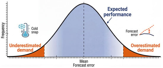
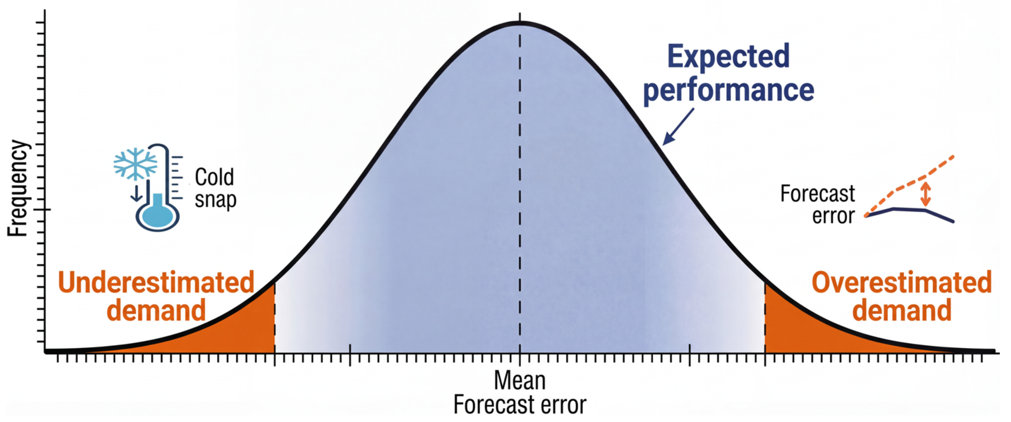
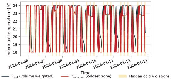
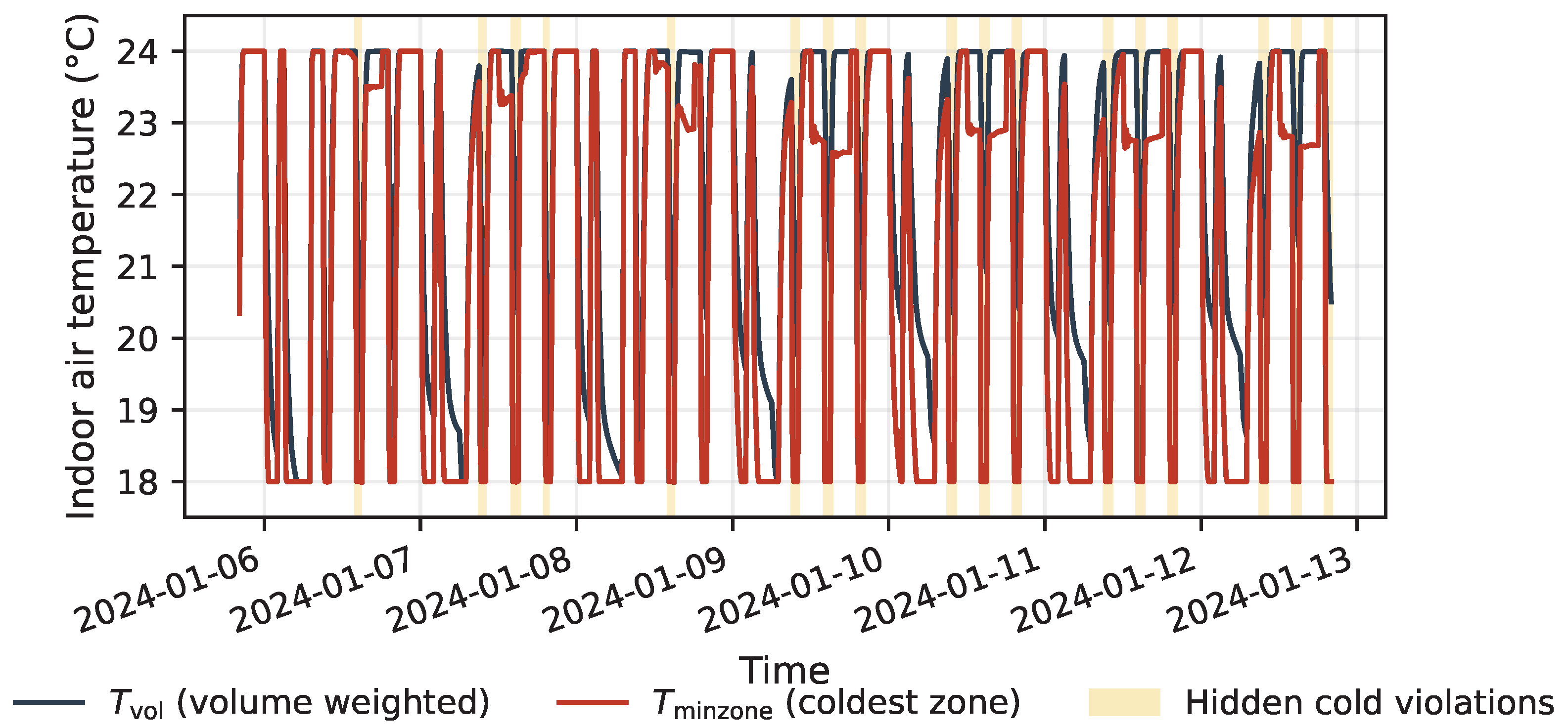
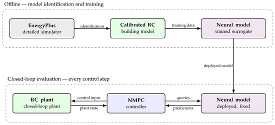
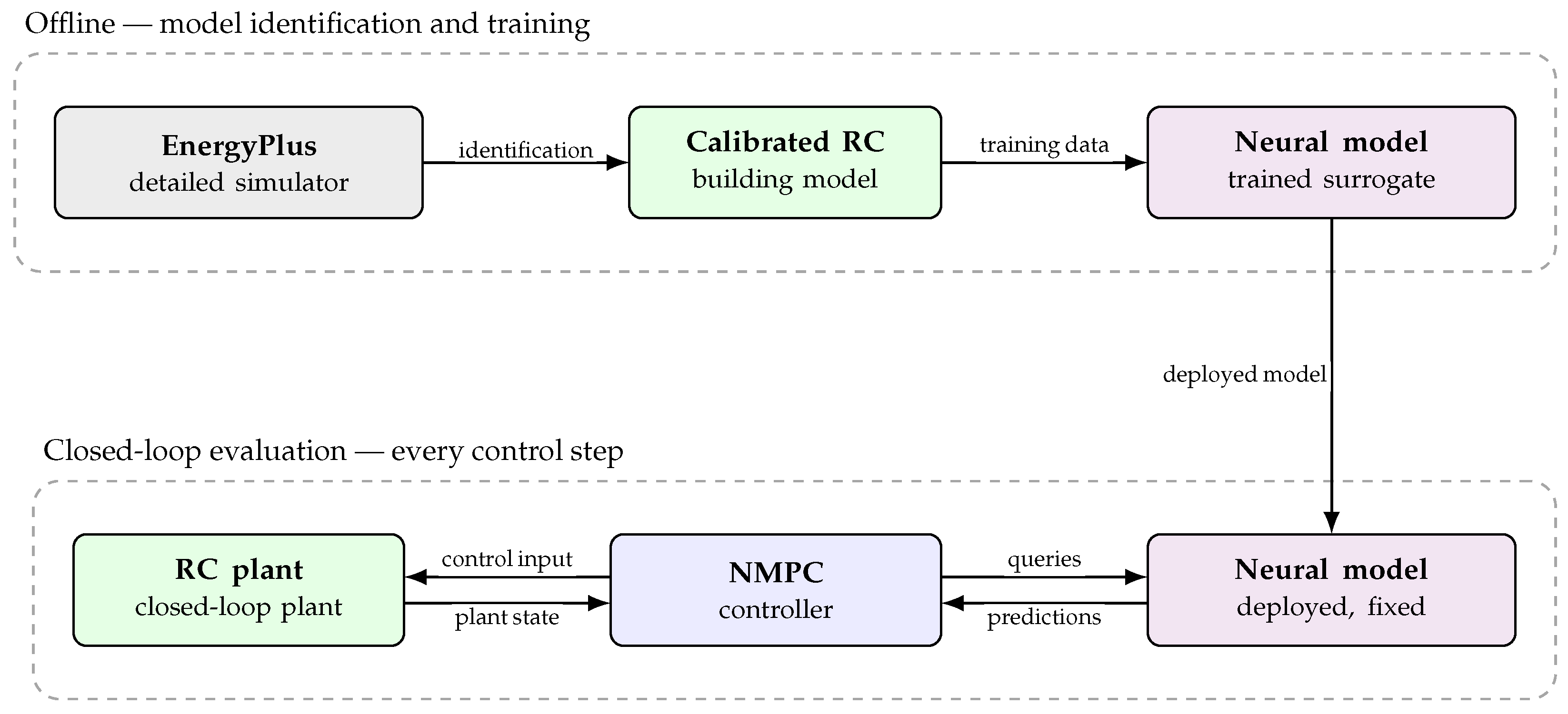
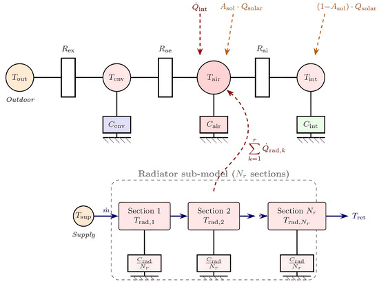
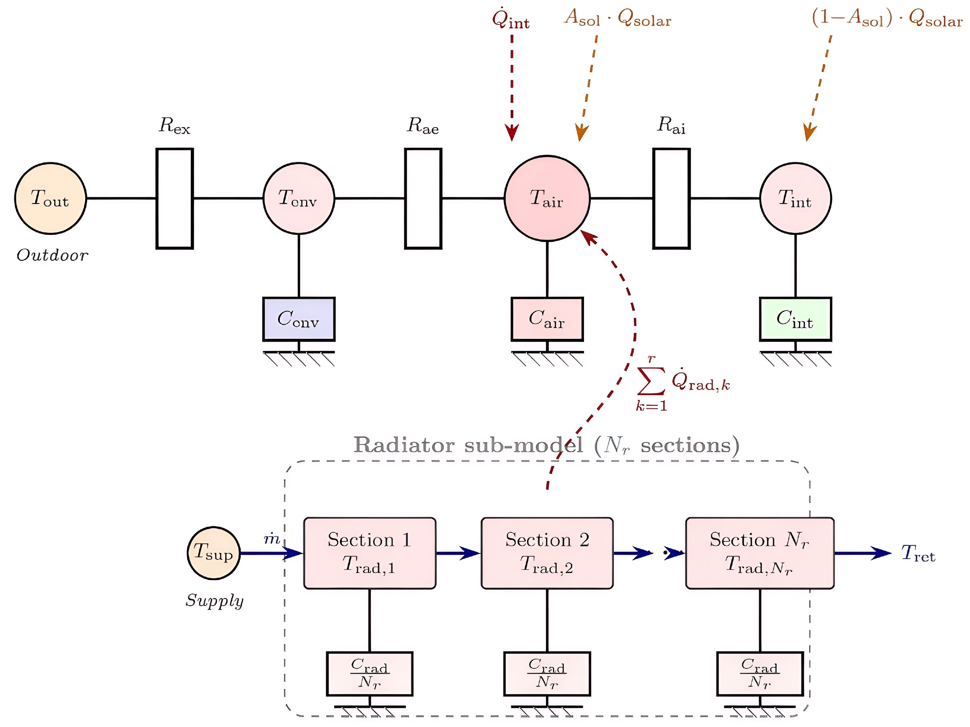
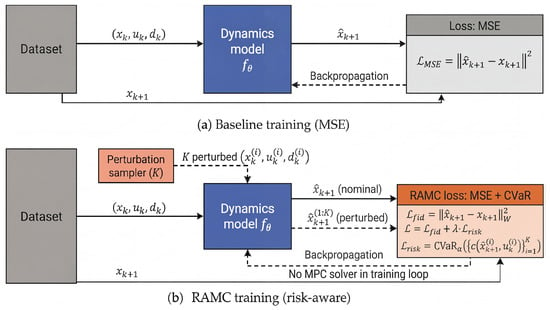
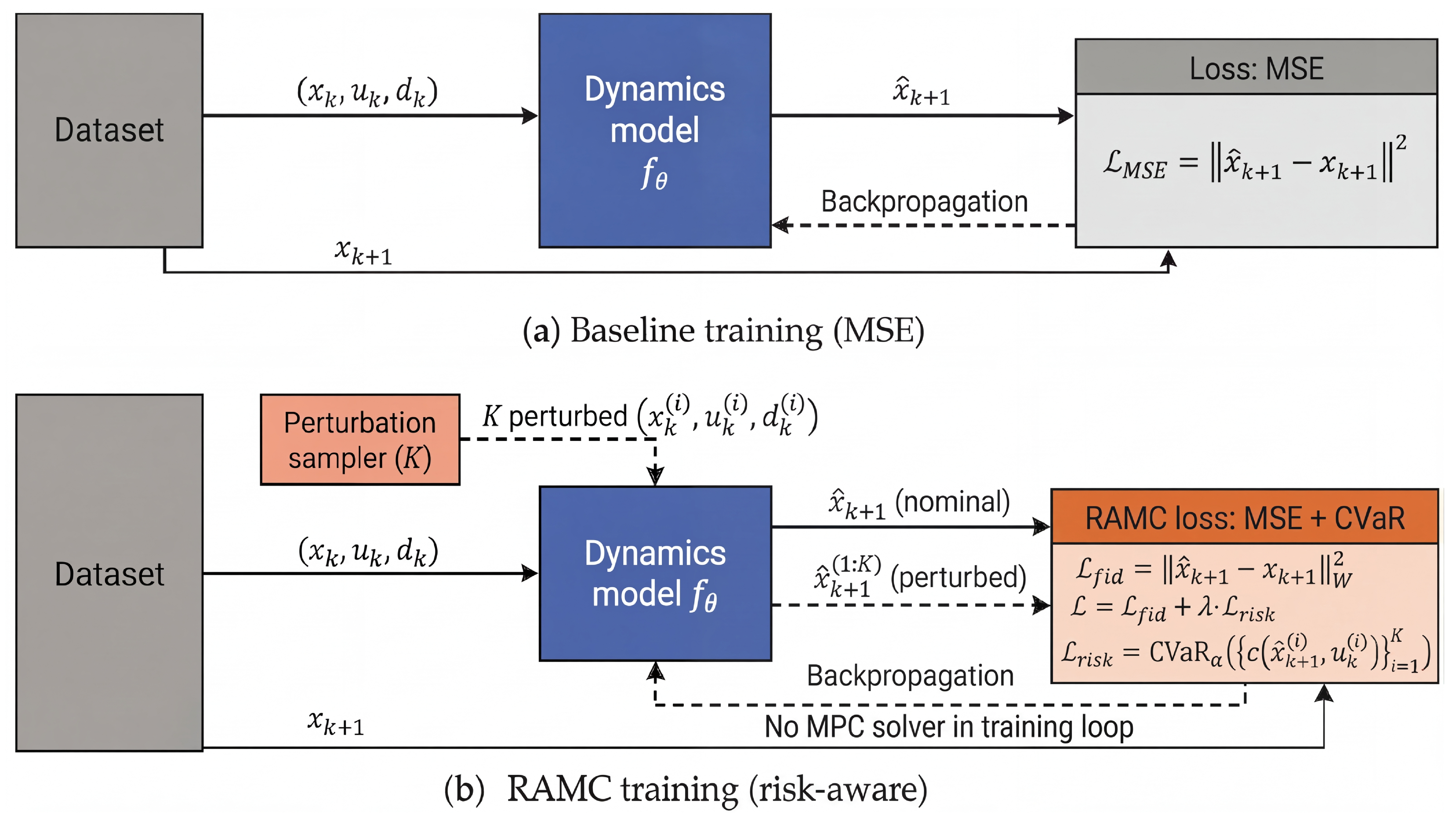
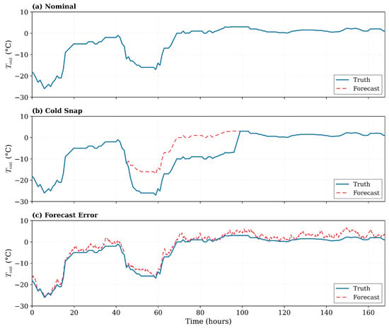
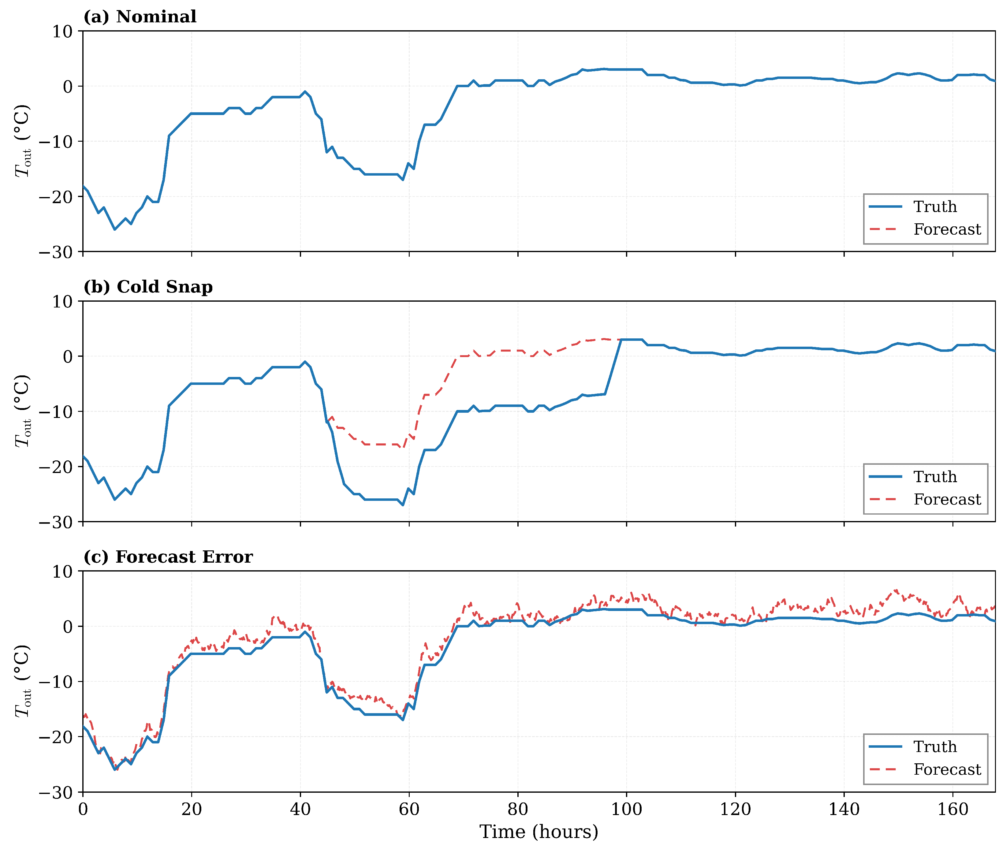
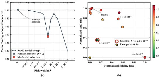
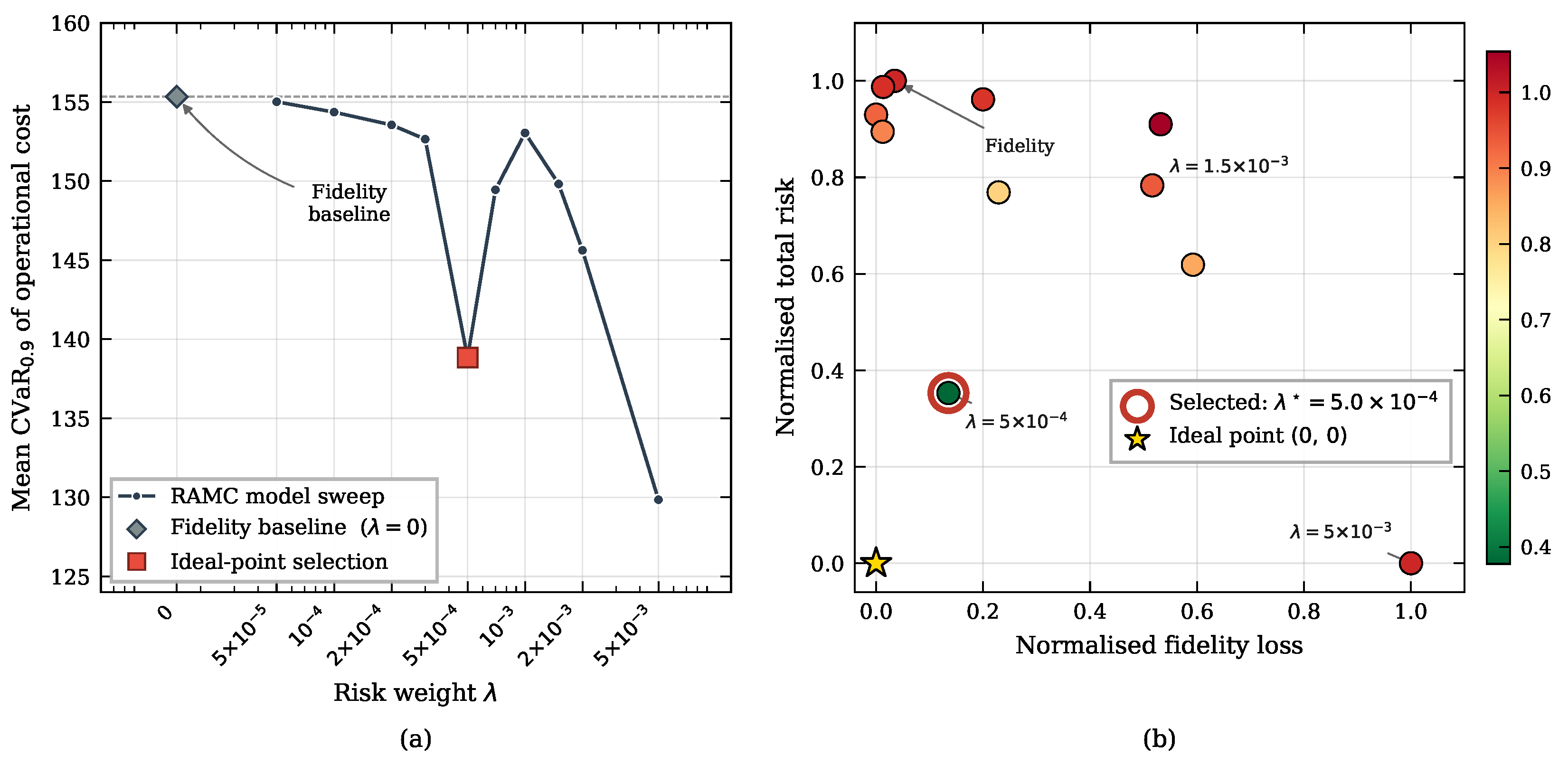
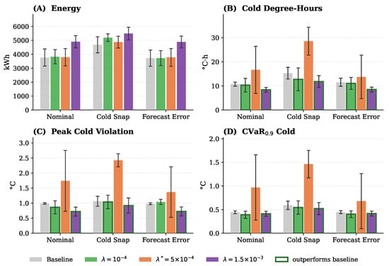
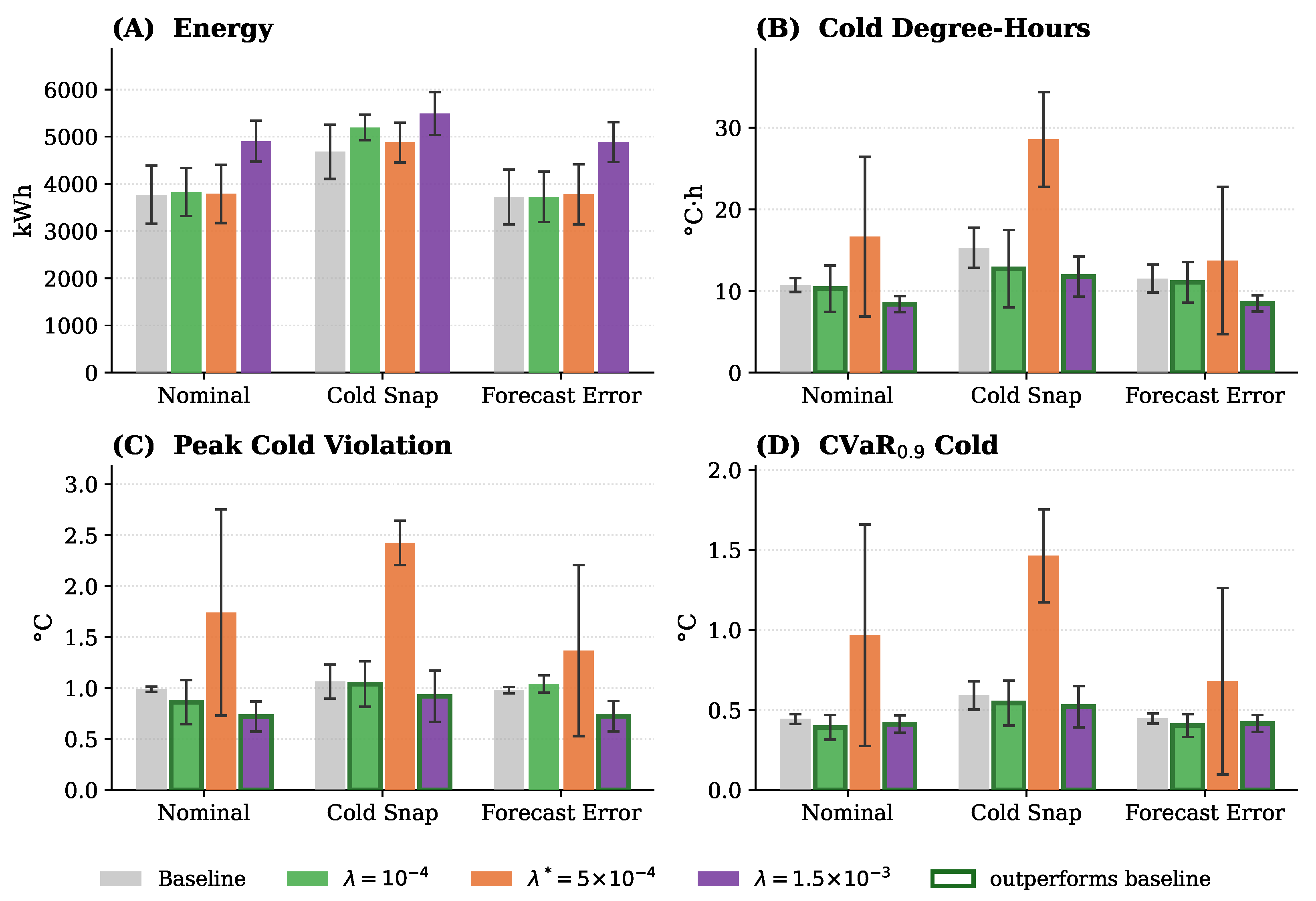
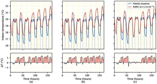
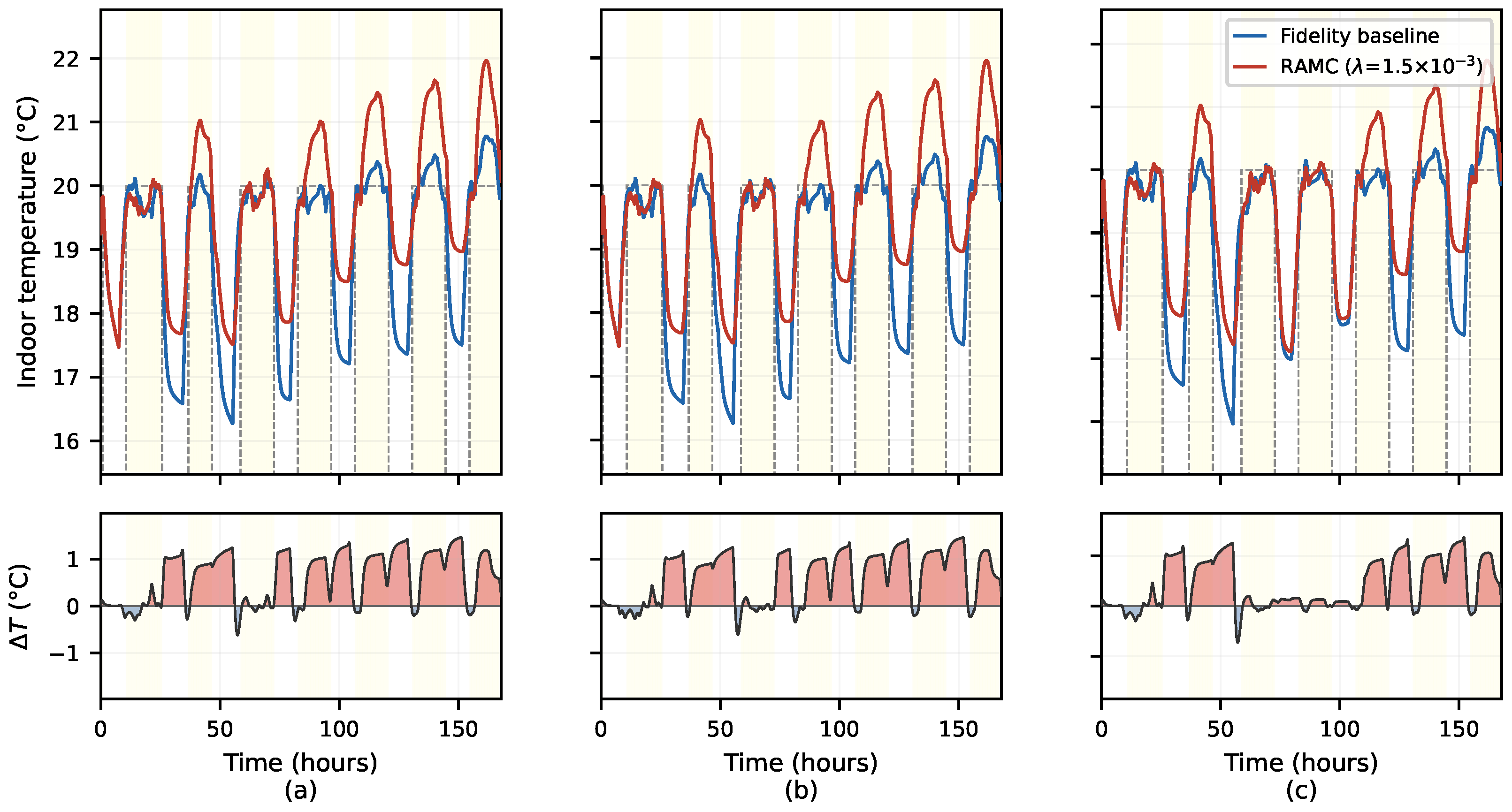
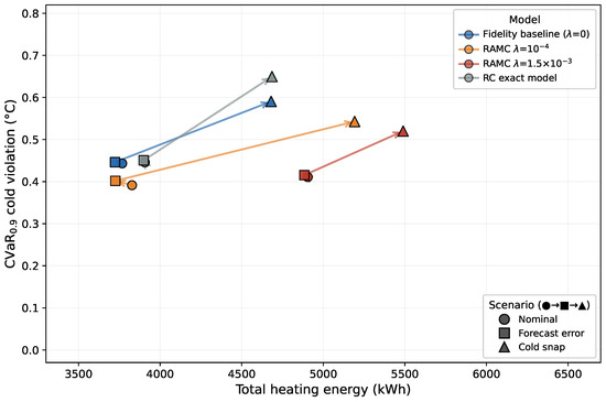
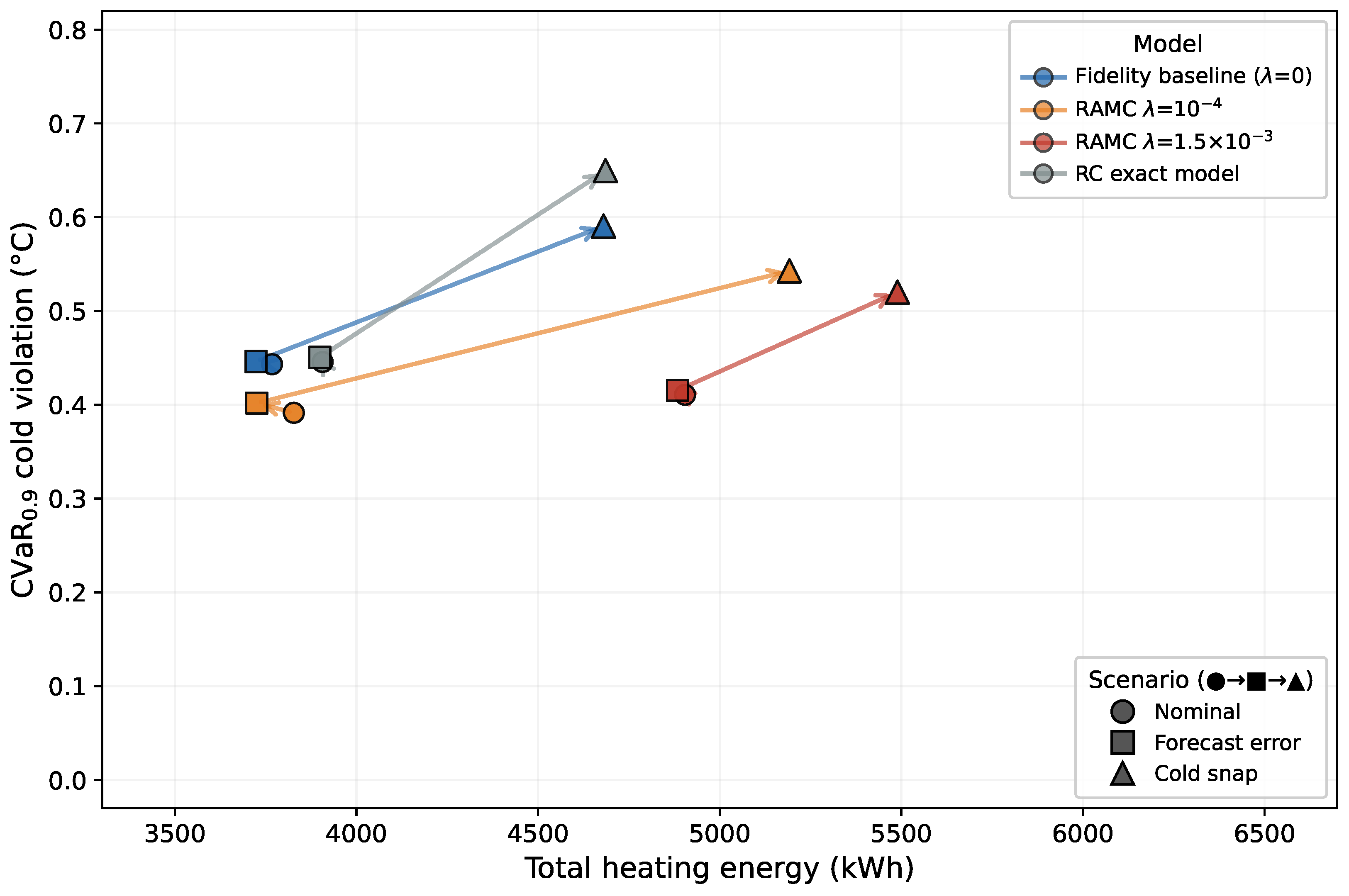
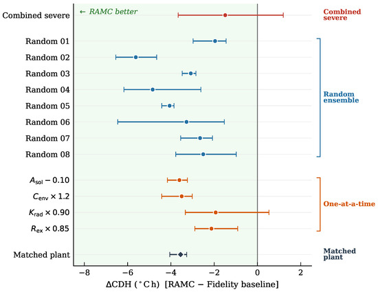
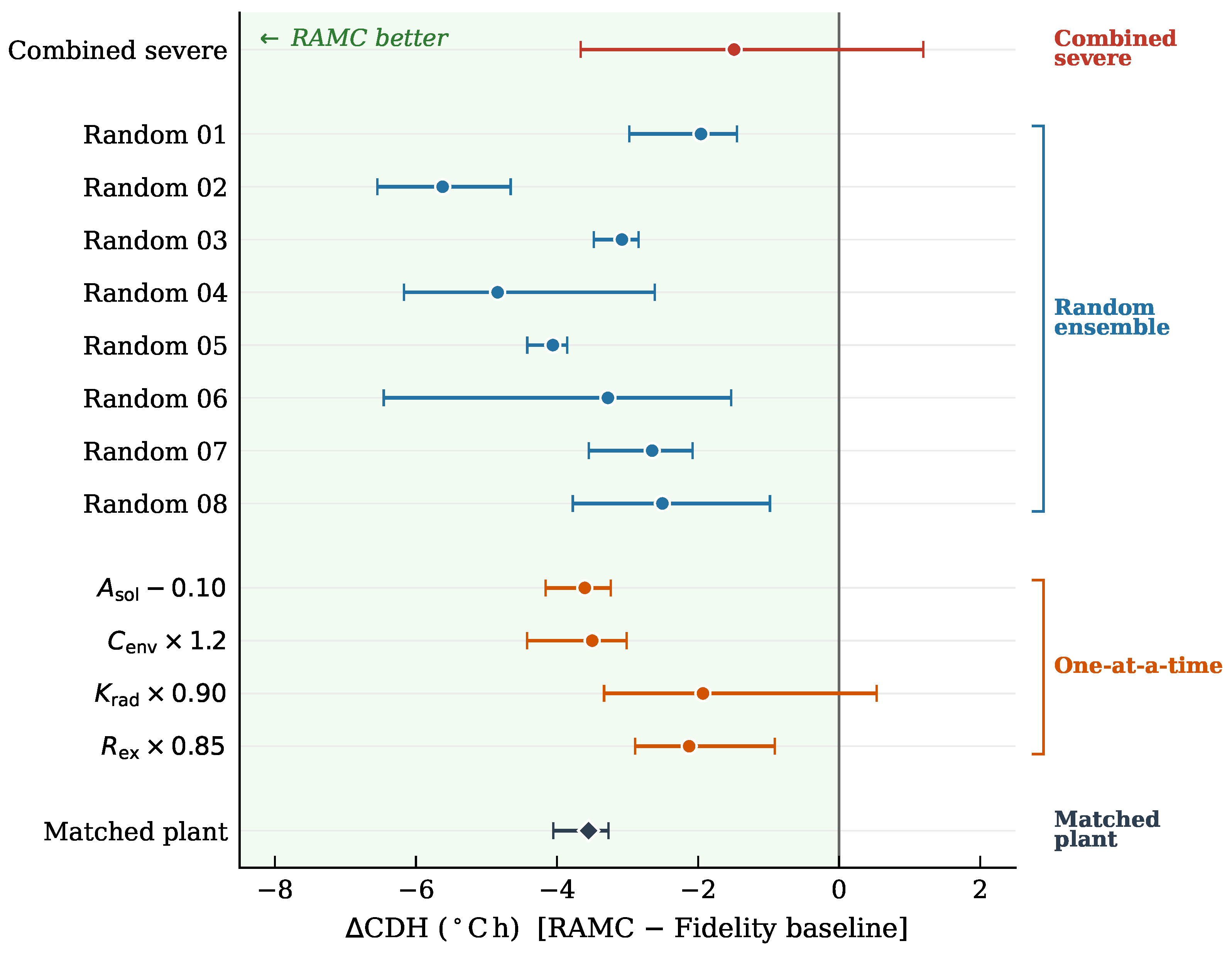
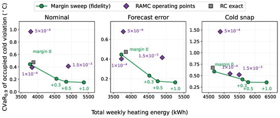
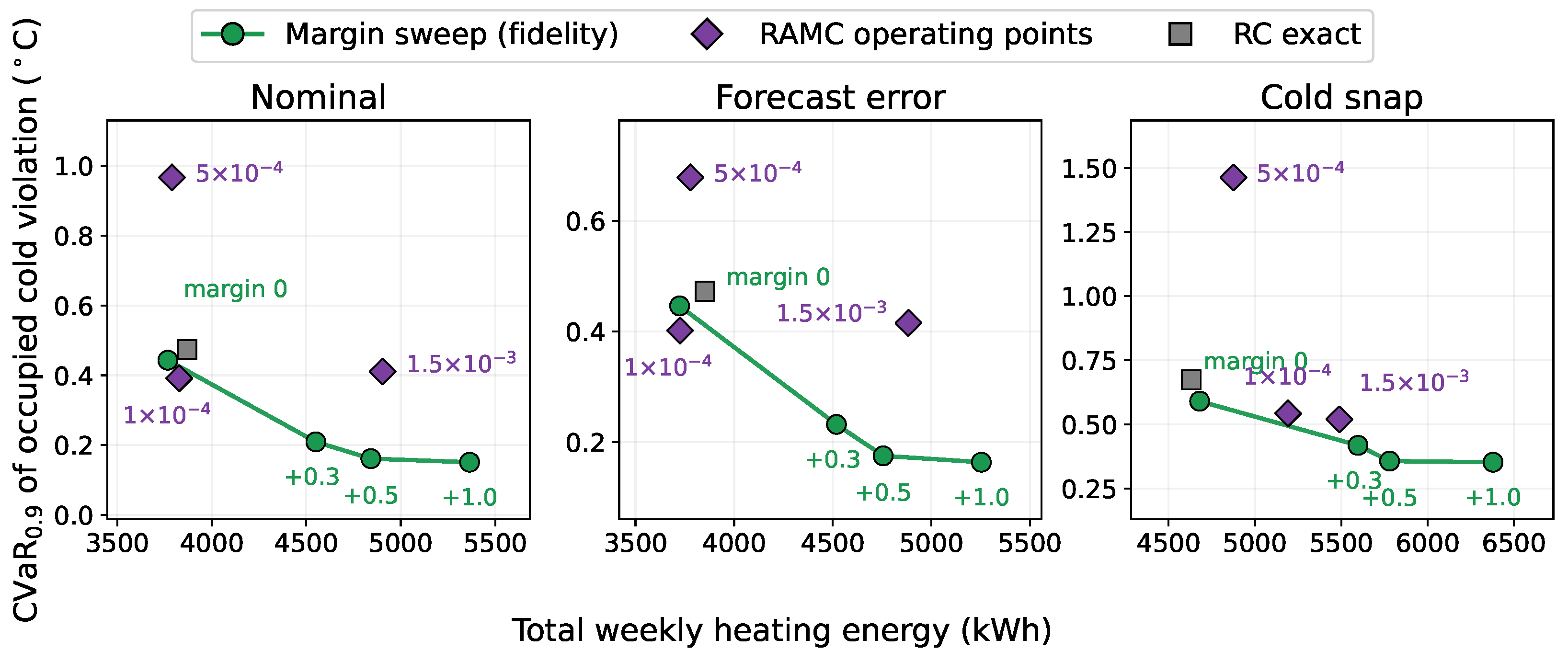

Disclaimer/Publisher’s Note: The statements, opinions and data contained in all publications are solely those of the individual author(s) and contributor(s) and not of MDPI and/or the editor(s). MDPI and/or the editor(s) disclaim responsibility for any injury to people or property resulting from any ideas, methods, instructions or products referred to in the content. |
© 2026 by the authors. Licensee MDPI, Basel, Switzerland. This article is an open access article distributed under the terms and conditions of the Creative Commons Attribution (CC BY) license.