


Abstract
In warm and humid tropical regions, balancing thermal comfort and energy efficiency presents a significant challenge due to high cooling demands. Strategies to reduce energy use and integrate renewable energy into buildings have increasingly focused on achieving self-sufficiency. Aligning with the United Nations Sustainable Development Goals 7 and 13, which call for access to sustainable energy and climate change mitigation, this study assessed the potential of facade-mounted solar photovoltaic (PV) systems to offset the cooling energy demand of buildings in the urban area of Quezon City, Philippines. A geospatial-computational workflow was developed utilizing QGIS 3.28 and Python 3.9 for LiDAR-derived 3D building model generation and hourly solar ray tracing. This workflow was used to estimate direct PV electricity generation and passive cooling effects from facade shading based on the ASHRAE radiant time series method. Results showed that east and west facades achieved the highest annual yields of up to 86 kWh/m2 and cooling load reduction by up to 7.3% due to the shading effect. Techno-economic analysis found several setups commercially viable, particularly installations on east–west walls with minimal self-shading and limited obstruction, focusing capital on the most productive surfaces. These findings support vertical solar PV as a complementary solution in dense tropical environments.
1. Introduction
Energy demand in the building sector accounts for approximately 43% of the global energy use and increases on average by 1% per year over the last decade under current policies, driven by population growth, economic development, and shifting climate conditions [1,2]. A substantial portion of this demand comes from cooling systems, which are often used to counteract high indoor temperatures caused by solar heat gains through building envelopes [3]. In tropical regions with warm and humid climates, such as the Philippines, achieving thermal comfort while maintaining energy efficiency presents a significant challenge, with up to 65% of building energy use attributed to ventilation and air conditioning systems [4]. Meanwhile, continued reliance on fossil fuels, which supply about 80% of global energy, accelerates resource depletion and contributes substantially to the world’s carbon footprint [5].
To meet increasing and variable electricity demand, the building sector has shifted toward energy-efficient and climate-responsive design strategies. The United Nations Sustainable Development Goals (SDGs), particularly SDG 7 and SDG 13, call for access to clean, sustainable energy and action to combat the effects of climate change [6]. In support of these, the Philippines’ Department of Energy (DOE) targets a 35% renewable energy (RE) share in the national generation mix by 2030 through the Philippine Energy Plan 2020–2040 [7]. The DOE also mandated the inclusion of energy efficiency measures in building design, with solar heat gain identified as a primary design consideration and photovoltaic (PV) systems encouraged as a preferred technology for reducing dependence on commercial power [8]. Given the country’s solar irradiation of 4.5–5.5 kilowatt-hours per square meter per day (kWh/m2/day) that exceeds the global average of 3.9 kWh/m2/day [9,10], solar PV technology emerges as a promising energy resource. Its integration into building envelopes offers opportunities to reduce cooling loads while expanding RE adoption in the built environment.
In dense urban areas, facades and rooftops of buildings are attractive for solving the issue of land use for solar PV deployment. While roofs receive significant solar radiation, space for PV modules is often constrained by existing infrastructure. Vertical facades, on the other hand, offer considerable surface area with increasing building heights and less susceptibility to dust accumulation [11,12]. Recent studies report vertical solar PV systems as a practical complement to rooftop installations, yielding up to three to four times the conventional output [11,12,13,14]. Simulation-based and experimental analyses in Southeast Asia indicate that walls facing east and west are optimal for vertical PV deployment, as these orientations align closely with peak solar irradiance [14,15]. However, much of this work has examined potential in temperate settings [11,13] or relied on simplified building geometries in tropical contexts [12,15], and the generation and passive-cooling benefits are often assessed separately [16,17]. In the Philippines, related studies have focused on rooftop or hybrid systems [18,19] rather than facades.
Installed on the building exterior, PV modules act as shading devices, limiting solar radiation absorbed by the envelope. This lowers exterior surface temperatures, mitigates indoor heat gains, and can decrease cooling loads by up to 70% [16,17]. This is a notable benefit given that cooling loads and solar availability are approximately in phase [20].
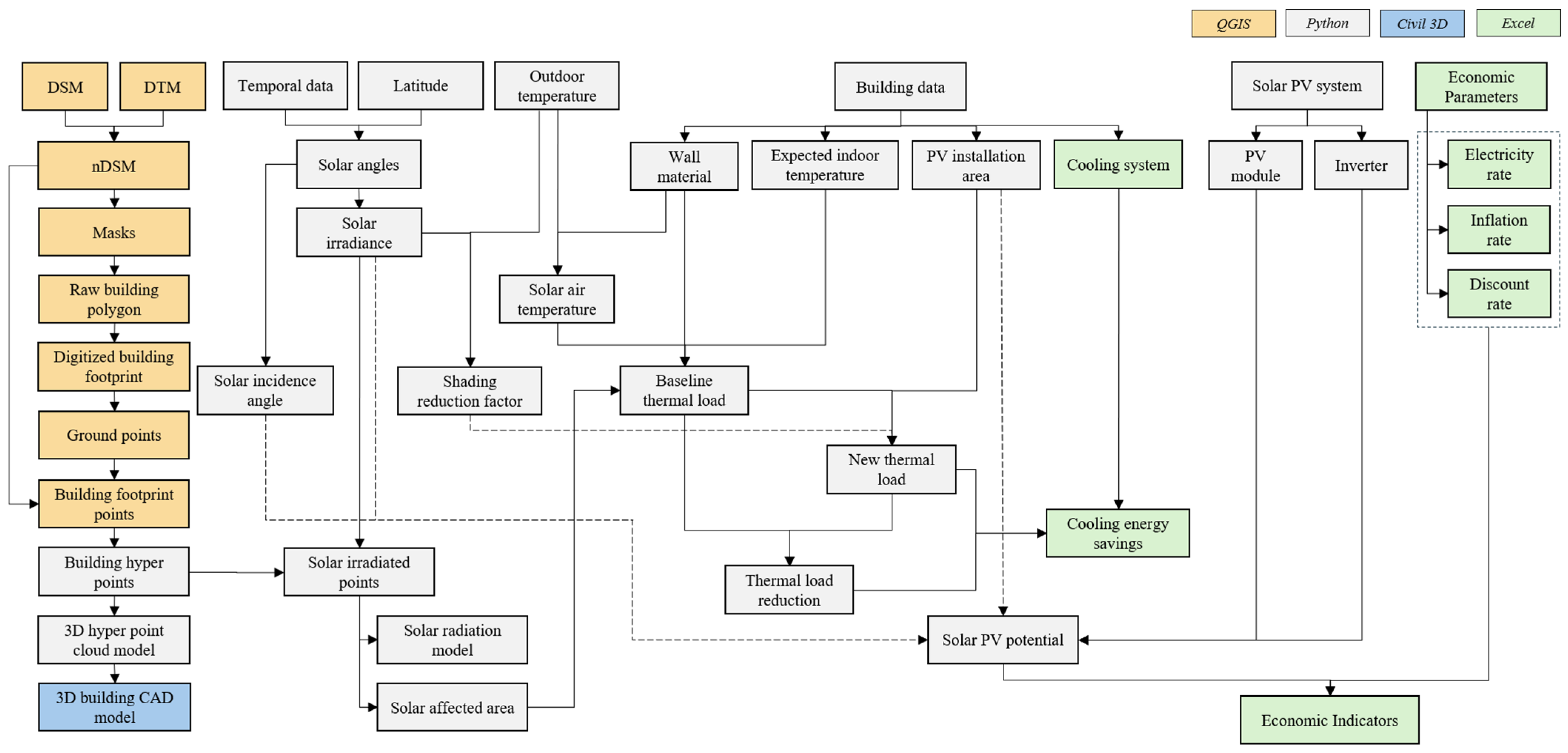
Therefore, this study focuses on the role of facade solar PV for self-sufficiency in the urban context of the Philippines. Its main objective is to assess the potential of vertically mounted solar PV systems and their thermal performance, particularly how these systems on the building envelope can supply a building’s cooling demand in a tropical area. This study specifically aims to (1) assess the power production potential of the installation; (2) evaluate the thermal performance in terms of heat gain reduction through shading; and (3) perform a techno-economic analysis of the system. This work extends a preliminary analysis presented at the 3rd International Symposium on One Health, One World (OHOW2024) [21], expanding the single-building case into a multi-building assessment with full techno-economic and thermal analysis. Figure 1 presents the conceptual framework, showing the inputs, analytical process, and resulting outputs. A more detailed version of the framework, mapping each processing step to its corresponding software environment, is provided in Figure A1 (Appendix A).
Figure 1.
Conceptual framework of the study.
2. Materials and Methods
The methodology mainly involves five stages: data acquisition, building model generation, solar radiation simulation, energy performance analysis, and techno-economic analysis. Figure 2 shows the key procedures, software used, and data outputs at each stage.
Figure 2.
General methodology of the study.
2.1. Site Context
Energy analysis was conducted on buildings located within the University of the Philippines (UP) Diliman, Quezon City, Philippines. The area is situated at 14°39′ N latitude and 121°03′ E longitude, within the Northern hemisphere and along the GMT+8 time zone. As shown in Figure 3a, monthly daytime temperatures in 2021 ranged from 26.3 °C to 30.8 °C, with global radiation values varying between 152 W/m2 and 525 W/m2 [22]. The solar analysis was conducted from 5:00 AM to 7:00 PM Philippine Standard Time (PST) on the first day of each month in 2021. This time frame accounts for variations in daylight before sunrise and after sunset in the study area, which occur around 5:25 AM and 6:29 PM, respectively [23]. It was determined that Quezon City receives approximately 12 h and seven minutes of daylight on average, with relatively longer day lengths from April to September (Figure 3b). Additionally, the area is reported to receive a solar photovoltaic power potential of approximately 4.5 kWh/m2/day [24], as shown in Figure 4.
Figure 3.
Monthly averages for climate parameters in Quezon City in the year 2021: (a) monthly mean maximum (dashed blue line), average (solid red line), and minimum (dotted blue line) air temperatures (°C) with monthly mean global solar radiation (W/m2, gray bars); (b) monthly solar schedule (gray shaded area) and solar noon time (solid red line) [20].
Figure 4.
(a) Solar PV power potential map indicating the location of the study area (adapted from [24]); (b) Global Horizontal Irradiation (GHI) levels in the Philippines and vicinity map of the selected buildings: Molave Hall, Melchor Hall, and Quezon Hall [24,25].
The study focused on three building types: (1) academic building: accessed at varying times throughout the day and night; (2) residential building: occupied continuously, 24 h a day, seven days a week; and (3) office building: typically used on a regular schedule from 8 AM to 5 PM, five days per week.
2.2. Building Descriptions
The selected academic building is Melchor Hall, which houses administrative offices, faculty rooms, classrooms, laboratories, organizations, and a library, all of which operate at varying hours of the day. Its longer side is oriented towards the north–south direction. Architecturally, Melchor Hall has an irregular footprint with projections and recesses, creating self-shading corners and partially enclosed areas. The five-story building has concrete walls with blank spaces on the east- and west-facing walls that can be potential sites for PV system installation (Figure 5).
Figure 5.
(a) East-facing walls of Melchor Hall; (b) west- and south-facing walls of Melchor Hall.
The selected residential building is Molave Hall, which functions as a dormitory. The building operates continuously, with occupant activities occurring throughout the day and night. It is a three-story concrete building with a symmetrical rectangular layout. Its wide facades are oriented north and south, while its east- and west-facing walls offer potential areas for solar PV system installation (Figure 6).
Figure 6.
(a) East-facing walls of Molave Hall; (b) west-facing walls of Molave Hall.
The selected office building is Quezon Hall. It serves as an administrative unit that supports university-wide operations, with activities occurring primarily during official working hours (8 AM to 5 PM) on weekdays. It is a three-story building with an elongated, almost bar-shaped footprint. Its design presents extensive east- and west-facing concrete walls and large columns, with north- and south-facing surfaces that present potential areas for solar PV system installation (Figure 7).
Figure 7.
(a) North-facing walls of Quezon Hall; (b) south-facing walls of Quezon Hall.
2.3. Data Sources
Spatial data obtained from Light Detection and Ranging (LiDAR) mapping in 2011 include various data derivatives provided by the National Mapping and Resource Information Authority (NAMRIA). Of particular interest to this study are two primary outputs containing elevation data: digital terrain model (DTM), which represents the ‘bare Earth’ excluding surface features; and digital surface model (DSM), which includes the heights of all surface features such as tops of buildings and trees [26]. Both the DTM and DSM cover the area of the selected buildings in UP Diliman, provided in 1 m raster resolution and in the EPSG:3123—PRS92/Philippines zone 3 coordinate reference system (CRS) [27].
Geographic information used to cross-reference and assist with the digitization of building footprints was sourced from the Esri satellite map and OpenStreetMap (OSM). The Esri basemap provided supplementary reference layers for the study area, including streets, satellite imagery, and topographic features [25]. OSM is a collaborative mapping platform where users contribute by manually digitizing features using aerial imagery, satellite navigation devices, field maps, and external datasets. The resulting vector data is available under an open data license [28].
Architectural data such as floor plans, elevation drawings, and relevant details of the selected buildings were requested from the Office of the Campus Architect in UP Diliman. The as-built drawings were used to guide the creation of the 3D building models, providing the general layouts of all floors, the roof, and the front elevation [29]. Since some sheets only had front views and floor plan dimensions, it was assumed that exterior dimensions were consistent across all floors.
Meteorological data were sourced from the Philippine Atmospheric, Geophysical and Astronomical Services Administration (PAGASA) Automatic Weather Station (AWS) in Science Garden, Quezon City, with hourly records from 6 AM to 6 PM spanning January to December 2021, the most complete dataset available at the time of the study [22].
Monthly electricity consumption data from January to December 2021, in kWh, were obtained for Melchor Hall and Molave Hall; however, corresponding records for Quezon Hall were unavailable for the same period [30]. These data, along with the 2021 tariff schedule obtained from the Manila Electric Company (Meralco) [31], were used in the techno-economic analysis to compute baseline electricity costs.
2.4. Computing System
All simulations and analyses were performed on a laptop computer equipped with the following specifications: an 11th Gen Intel® Core™ i5-1135G7 processor (2.40 GHz), 16.0 GB of RAM, and a 64-bit operating system on an x64-based processor.
2.5. Software
The open-source geographic information system Quantum GIS (QGIS) 3.28, which is available for free, was used to visualize and process spatial data [32]. The core plug-in utilized was the Processing Plugin, along with command-line tools from the Geospatial Data Abstraction Library (GDAL) for processing vector and raster data.
For general computation, data analysis, and processing, the free and open-source programming language Python 3.9 was used [33]. Key modules used include PySolar (0.13), Plotly (6.8.0), Shapefile (pyshp 3.1.3), NumPy (2.0.2), Pandas (2.3.3), GeoPandas (1.0.1), Shapely (2.0.7), Matplotlib (3.9.4), and SciPy (1.13.1).
PySolar is an open-source Python library designed for solar energy calculations and PV modeling. It uses VSOP87 theory, a mathematical model of planetary positions and motions, to compute solar altitude, azimuth, and zenith angles. PySolar calculates direct irradiance in W/m2 using a clear-sky model, assuming minimal atmospheric absorption or reflection, and accounting for scattering [34].
2.6. DSM Normalization
The following subsections use the dataset for Melchor Hall as an example to illustrate the procedures involved. In the QGIS Processing Plugin, the Build Virtual Raster tool was used to create virtual layers for both the DTM and DSM. Using the QGIS Raster Calculator, the normalized digital surface model (nDSM) was derived by applying the formula ‘DSM − DTM’. The resulting nDSM contains the height information for all features within its spatial extents (Figure 8).
Figure 8.
Raster outputs derived from LiDAR: DSM (top left), DTM (bottom left), and nDSM (right).
2.7. Building Footprint Extraction
The building footprints were digitized using a semi-automated approach combining raster and vector tools in QGIS [35]. A mask was created using the Raster Calculator with the formula ‘nDSM > {height}’, where the height threshold was initially determined to be around 10 m by trial and error to best represent the building’s shape (Figure 9). The GDAL Polygonize tool was then used to convert the resulting raster mask to a vector layer, which was then visualized with adjusted symbology (low opacity) over the Esri satellite map for comparison (Figure 10a). An additional mask using an 11 m threshold was generated, as it provided clearer building boundaries (Figure 10b).
Figure 9.
nDSM layer after application of height threshold.
Figure 10.
(a) nDSM vector layer set to 50% opacity (yellow), overlaid on Esri map; (b) tracing of footprint using various layers.
A new shapefile was initialized, set with a Polygon geometry type and EPSG:4326—WGS 84 CRS for compatibility with other datasets, as it is a globally adopted geospatial standard. With snapping options enabled, the building footprint was manually traced using the Add Polygon Feature tool, with multiple layers of varying symbology used as reference. The Vertex Tool was then used to refine individual polygon points for precision.
2.8. Feature Comparison
The building’s digitized footprint was subsequently compared with that from OSM. As expected, a spatial offset exists between the two datasets, attributable to the difference in coordinate systems, as the building footprint was reprojected from the nDSM referenced in PRS92, while OSM uses WGS 84. The accuracy of the digitized footprint was therefore assessed against the architectural drawing: the digitized footprint of Melchor Hall measured approximately 3640.79 m2, closely matching the 3636.37 m2 obtained from the architectural drawing, a difference of about 0.12%.
2.9. 3D Building Model Generation
Using the Regular Points tool in QGIS, a regular grid of points with 1 m spacing was generated across the building footprint’s spatial extent and clipped using the Clip algorithm to retain only points within the footprint. The Add X/Y Fields to Layer tool was applied to assign coordinate fields in both PRS92 (renamed ‘xcoord’ and ‘ycoord’) and WGS 84 (renamed ‘Longitude’ and ‘Latitude’). Elevation and height values were then extracted from the DTM and nDSM, respectively, using the Sample Raster Values tool, and the final layer was saved as a shapefile.
A Python script automated the conversion of the 2D building points into a 3D hyper point cloud. The script imports essential libraries (Shapefile, Datetime, Matplotlib), reads the shapefile containing building point data, and extracts the coordinates, elevation, and height for each record. It then generates hyper points by extruding each point vertically along the building’s height at 1 m intervals, storing these points in a list, until all records are processed. The resulting data are written to a new shapefile and visualized as a 3D scatter plot using Matplotlib (Figure 11).
Figure 11.
3D hyper point cloud using Matplotlib in Python.
2.10. Building Surface Area Estimation
The surface area of each building facade was estimated using Autodesk Civil 3D 2024, a computer-aided design (CAD) software, where the boundaries of the 3D hyper point cloud were traced to define the dimensions of each building facade (Figure 12a,b). Given the 1 m spacing of the hyper points along the x-, y-, and z-axes, the length of each line connecting adjacent points was used to calculate the surface area.
Figure 12.
(a) 3D building model visualized and traced in Civil3D; (b) measuring the area of each surface in Civil3D.
To create the CAD model from the building points, several assumptions were made: the outermost points at each corner were treated as the vertices for the building walls, and all angles between the walls were assumed to be right angles, meaning all lines were considered perpendicular to each other. These assumptions simplify the modeling process but may introduce slight deviations from the building’s actual non-orthogonal and irregular lines, which can arise during construction. After generating the model, the areas of all walls oriented in the same direction were then aggregated.
2.11. Calculation of Solar Angles
The solar declination angle (°) is the angle between the line connecting the Earth and the Sun, and the equatorial plane, varying with the day of the year [36]. For most engineering purposes, it can be sufficiently approximated using Equation (1) [37]:
The hour angle (°) is the angular displacement of the Sun east or west of the local meridian due to Earth’s rotation, where each hour corresponds to an angle change of 15°, with 0° at 12 o’clock (noon). It is given by Equation (2) [36]:
where is the solar time in hours.
The solar altitude (°) is the angle between the Sun and a plane tangent to the Earth. Equation (3) relates this parameter to latitude (°), , and [37]:
The solar azimuth (°) can be determined using Equation (4) or Equation (5) [37]. The sine equation captures the east–west component of the Sun’s position, while the cosine equation, which includes the latitude, accounts for the north–south component:
2.12. Solar Radiation Simulation
Solar radiation incident on building surfaces was simulated to determine sunlight availability, which is essential for calculating both thermal load and solar PV potential of the building. This study estimated solar radiation using a clear-sky radiation model following [14] and using PySolar, which calculates direct irradiance and accounts for scattering and partial reflectance contributions [34]. Among the three components of incident solar radiation, direct radiation generally has the highest share, while reflected radiation contributes the least due to the low albedo or reflectivity of Earth’s natural surfaces, meaning that most sunlight is absorbed rather than reflected [36].
The simulation was implemented through a Python script following these main steps: (1) the script imports NumPy, Pandas, GeoPandas, and PySolar, and sets relevant parameters, including file paths, location coordinates, and date and time details. (2) The script accesses the shapefile containing building hyper point data and extracts the relevant building model attributes. (3) After converting time to Coordinated Universal Time (UTC), the script computes the solar altitude and azimuth using PySolar’s solar.get_altitude() and get_azimuth() functions, respectively, taking the building’s geographic coordinates and time as inputs. (4) Using the solar angles converted to radians, the Sun’s direction vector (altitude, azimuth) is computed for each hour of analysis. SciPy’s KDTree algorithm is then applied to perform ray tracing on the hyper point cloud, identifying sunlit points and computing irradiance based on the date and solar altitude. (5) Sunlit point coordinates and corresponding irradiance values are compiled into a GeoDataFrame and saved as comma-separated values (CSV) files. For each building facade and roof, the number of sunlit points and average hourly irradiance are likewise recorded. A 3D scatter plot is generated using Plotly to display both the building points and sunlit points, illustrating the solar exposure on the building (Figure 13).
Figure 13.
3D scatter plot of the building model at 8:00 AM, generated using Plotly in Python.
2.13. Building Thermal Load Calculation
The solar-air temperature (°C), an input parameter for estimating building thermal load, was calculated using the following formula [37]:
where (°C) is the outdoor air temperature, (dimensionless) is the solar radiation absorptance, (W/(m2K)) is the convective heat transfer coefficient, (dimensionless) is the surface emissivity, and (W/m2) is the net long-wave radiation, or the difference between long-wave radiation and the radiation emitted by a blackbody at outdoor temperature. Design values for were based on dry-bulb temperature representing peak sensible ambient conditions, derived from monthly average data from the PAGASA AWS in Quezon City. The total incoming solar irradiance (W/m2) was taken as the average of all solar radiation incidents on each surface. The was set to 0.60 for concrete [37]. The ratio of the solar radiation absorptance to the heat transfer coefficient for convection over the building, , varies from 0.026 m2°C/W for light-colored surfaces to a maximum of about 0.053 m2°C/W [38]. The correction factor ranges from 0 °C to 4 °C depending on surface orientation, and is assumed as 0 °C for vertical surfaces [37].
Thermal load at the exterior walls and roofs was defined by the conduction formula in Equation (7) [37]. The building thermal load is the energy required to maintain a specific indoor temperature in comparison to the outdoor temperature, with the assumption that the full thermal gradient is inherently addressed by air conditioning. The base thermal load of the building (without PV modules) was calculated hourly using
where (kWth) is the baseline thermal load and (W/(m2K)) is the overall heat transfer coefficient dependent on the structural material. It was set to 6.303 W/(m2K) for concrete, adopted from the thermal load estimation study for buildings in UP Diliman [39]. That study modeled an 8-inch concrete masonry unit, the standard wall material in the country under Presidential Decree No. 1096, the National Building Code of the Philippines. This value reflects an uninsulated concrete wall assembly typical of tropical construction, where thermal insulation is generally omitted, resulting in higher -values than the insulated envelopes common in temperate climates. The area of the building surface (m2) affected by solar radiation was taken from the results of solar radiation modeling. The indoor air temperature was assumed to be 24.4 °C, based on studies conducted on buildings in tropical regions [40]. Walls were assumed to be fully opaque, with openings excluded from the simulation. This simplification has also been adopted in prior facade–PV assessments, which treated entire building surfaces as opaque solar collectors [12].
2.14. Solar PV Potential Estimation
The power output of a solar PV system is directly proportional to the solar irradiance at a given site [36]. Given the hourly isolation and module specifications, the potential power output was estimated using the formula [41]:
where (kW) is the instantaneous solar PV potential measured hourly, (W/m2) is the solar irradiance, (%) is the module efficiency, (m2) is the total area of solar PV installation, and (%) is the inverter efficiency. The PV modules are assumed to match the inclination and orientation of their respective building surfaces, with facade-mounted panels considered vertical. The power production potential of grid-connected, wall-mounted solar PV systems was assessed through calculated solar positions and irradiance on the first day of each month. The solar incidence angle is the angle between the incoming solar rays and the surface normal. It varies throughout the day based on the tilt, surface solar azimuth, and solar altitude, given by [37]
where (°) is the surface solar azimuth angle, or the angular difference between the solar azimuth and the surface azimuth (°), and (°) is the tilt angle of the solar PV module. In the case of a vertical surface ( 90°) with any orientation, such as the outer walls of building envelopes, Equation 8 can then be simplified as in Equation (9):
The surface azimuth angle is dependent on the orientation of the surface of the PV module. Table 1 shows the different values of ψ for common orientations [37].
Table 1.
Surface orientations and corresponding azimuths, measured from north.
The average daily PV yield in month (kWh/day) was then calculated as in Equation (10), where (kW) is the mean of all non-zero hourly outputs, and (h) is the average sunshine duration during the same month:
The annual PV energy generation (kWh/yr) was computed by taking the sum of the average daily yield (kWh/day) for each month , then multiplied by the number of days in the same month:
2.15. Solar PV Characteristics
The analysis used the JAM72S20-440 monocrystalline solar module, which delivers 440 watt-peak (Wp) under standard test conditions (STC) [42]. Each module has an area of 2.56 m2 and a conversion efficiency mod 19.7% (Table 2). The inverter has an efficiency of 97.6%, based on the SUN-5K-SG04LP1-EU-SM2 model. All system components were identified to be available in the country at the time of analysis.
Table 2.
Technical characteristics of solar PV system.
2.16. PV Installation Cases
In reality, given the current and expected costs of PV modules, fully covering all building facades would not be a practical approach. Therefore, three installation configurations were considered. Most buildings typically have at least two exposed facades with opposite orientations, which provide potential areas for PV placement.
For the selected buildings, the front is defined as the longer, street-facing side. Facing that front, Case A corresponds to the installation at the right-hand side of the building, Case B to the left-hand side, and Case C combines both left and right sides (Figure 14). Each case is further subdivided into three subcases to reflect progressively smaller installation areas. Subcase 1 considers all vertical surfaces facing the designated direction (including recesses and projections), Subcase 2 is limited to the major side walls only, while Subcase 3 excludes surfaces with obstructions such as windows or openings. Gray areas represent building surfaces, blue indicates installable PV areas, and hatched blue marks excluded areas due to obstructions.
Figure 14.
PV installation cases (top) and subcases (bottom), as viewed from the front: Case A (right side), Case B (left side), and Case C (both sides). Subcase 1 considers the whole facade, Subcase 2 is limited to the major wall panels only, and Subcase 3 excludes obstructions.
2.17. New Building Thermal Load Estimation Due to PV Installation
With the assumption that there is sufficient clearance beneath the panels for ventilation, heat transfer is reduced primarily through shading, while the -value of the envelope is assumed unchanged. Derived from Equation (7), the new thermal load on the building surfaces with PV modules was approximated using
where (kWth) is the new thermal load after PV installation, (m2) is the portion of the solar-affected area that is not covered by PV modules, while (m2) is the portion of covered by PV modules (Figure 15).
Figure 15.
Schematic representation of thermal load calculation after PV installation. The yellow region represents the total surface area exposed to the Sun, . The blue panels denote the PV-covered areas , which contribute to the total covered area , while the remaining yellow portion indicates the uncovered area .
The shading reduction factor represents the average percentage of heat reduction from the shade of fully installed PV modules under varying ambient temperatures and solar irradiance ranges, adopted from [3] on building heat gain reduction from grid-connected PV systems in the same tropical climate zone (Table 3).
Table 3.
Average percentage of heat reduced by the shade of PV modules at varying ambient temperatures and solar irradiance ranges.
The daily thermal energy for month (kWhth/day) was taken as the average hourly thermal load (kWth/day) multiplied by the average sunshine duration (h):
2.18. Thermal Load Reduction Due to PV Installation
The annual thermal energy (kWhth/yr) was then computed by taking the sum of the average daily energy (kWhth/day) for each month , then multiplied by the number of days in the same month:
The thermal performance of the PV installation was evaluated by comparing the building’s thermal load before and after installation, with the thermal load reduction defined as and expressed as
2.19. Cooling Load to Electricity Conversion
Thermal loads computed in Section 2.17 were converted into cooling electricity demand based on the operational periods and the assumed coefficient of performance () of the air conditioning systems. Thermal loads in this study are attributed to solar heat gains, with air conditioning assumed to operate primarily to maintain indoor comfort during periods of solar exposure. For this reason, the analysis limits air-conditioning operating hours within the bounds of sunshine duration, as presented in Table 4.
Table 4.
Building use profiles and assumed air-conditioning analysis periods.
The cooling energy savings (kWh/yr) was calculated as factored by the analysis period over sunshine duration, then divided by the of the air conditioner:
The (dimensionless) is a measure of the efficiency of a cooling system, defined as the ratio of cooling output (amount of heat removed) to the electrical power input (net energy supply). Typically, values are greater than 1, with higher indicating better energy efficiency and reflecting a smaller difference between indoor and ambient temperatures. In this study, the was derived from an average energy efficiency ratio () of 10.3, measured from air conditioners at UP Diliman [4]. The relationship between and is defined as follows:
2.20. PV Contribution to Cooling Demand
The following metric contextualizes the role of solar PV in meeting energy demands associated with cooling, expressed as a percentage of the estimated solar PV energy relative to the new cooling electricity demand :
2.21. Techno-Economic Analysis
A techno-economic analysis was performed to determine the commercial viability of facade-mounted solar PV integration. The system components were selected based on commercial availability in the Philippines and specifications used in recent local studies. The proposed system consists of JAM72S20-440 monocrystalline solar PV modules connected to a SUN-5K-SG04LP1-EU-SM2 inverter.
A unit cost of 1.15 USD/Wp for system installation was adopted, which reflects recent price benchmarks for grid-connected solar PV systems in the Philippines. Higher costs accounted for the added structural, labor, and mounting complexity required for vertical facade applications. This unit cost covers both direct costs (modules, inverter, BOS, mounting, labor) and indirect costs (engineering, permitting, taxes, installation overhead). The solar PV modules are expected to operate over a 25-year project lifetime, and are assumed to degrade gradually, reaching a final output of 80% of their rated capacity by end-of-life. The inverter is assumed to be replaced once in year 15 at a cost of 0.22 USD/Wp. Operation and maintenance () costs were estimated at 1% of the total capital cost annually, equivalent to 0.011 USD/Wp/yr.
The site is connected to the Meralco electricity grid, with a retail electricity price of 0.1807 USD/kWh, based on the 2021 average. Financial assumptions include a 49.25 PHP/USD exchange rate and a 4.5% inflation rate based on the Bangko Sentral ng Pilipinas [43,44], and a 10% discount rate, in line with the social discount rate prescribed by the National Economic and Development Authority for infrastructure projects [45]. All cash flows were adjusted for inflation where applicable and discounted to present value for economic evaluation.
2.22. Annual Electricity Cost Savings
The annual electricity cost savings (PHP/yr) were derived by multiplying the monthly electricity savings by the grid electricity rate (PHP/kWh), which allows annual cost savings to reflect seasonal variations in both energy use and utility prices.
2.23. Levelized Cost of Electricity
To assess the economic feasibility of vertical solar panel installation, the levelized cost of electricity () was calculated as the ratio of the present value of total system costs to the present value of total electricity generation over the project lifetime. It also serves as a normalized metric to compare PV-generated electricity against the grid electricity price [46]. The was computed using the discounted cash flow approach:
where (USD/yr) is the total cost in year , including capital investment, annual , and inverter cost. (kWh/yr) is the annual energy production, accounting for module degradation. (%) is the discount rate, is the year, and (yr) is the project lifetime. For the calculations, the capital cost was estimated based on the installed system cost of 1.15 USD/Wp, while costs were 0.011 USD/Wp/yr (1% of capital), and the inverter replacement cost of 0.22 USD/Wp was applied once in year 15. The nominal discount rate was set to 4.5% with a project lifetime of 25 years.
2.24. Simple Payback Period
The simple payback period () estimates the time (yr) needed to recover the initial capital investment through annual electricity cost savings, calculated as
where is the initial capital cost of the system, based on an installed cost of 1.15 USD/Wp, and is the annual electricity cost savings, including both PV energy offset and cooling electricity savings.
2.25. Net Present Value
Net Present Value () quantifies the overall financial return of the vertical PV system by comparing the present value of cumulative benefits against the total capital and replacement costs over the project lifetime. is calculated as
where is the electricity cost savings, is the total cost in year , is the discount rate, and is the project lifetime.
2.26. Sensitivity Analysis Setup
The sensitivity analysis investigates the influence of four key economic parameters on the techno-economic performance of vertical PV systems: installation cost, inflation rate, discount rate, and PV degradation rate. Each parameter was varied by ±20% from the base input value to preserve the technical viability of grid-connected solar PV, and the effect was observed on three metrics: , , and .
3. Results
3.1. Local Solar Analysis
3.1.1. Solar Angles
Solar declination was computed for the first day of each month in 2021 (Figure 16a). The plot shows that solar declination starts at −23.01° in January and remains negative until March. In April, it turns positive, peaking in July at 23.12°. Then, the declination values gradually decline back to negative from September to December, reaching −22.11° in December. This pattern reflects the seasonal changes driven by the Earth’s tilt and orbit.
Figure 16.
(a) Monthly solar declination (2021); (b) hour angles from 5 AM to 7 PM.
Hour angles were measured from 5:00 AM at −105° to 7:00 PM at 105°. Figure 16b shows that before noon, the negative hour angles indicate the Sun is positioned east of the building’s meridian, which is an imaginary reference line that runs vertically through the center of the building. At noon, the hour angle reaches zero, meaning the Sun is at its highest point in the sky. In the afternoon, hour angles are positive, which shows that the Sun has moved west of the building’s meridian.
Solar altitudes were calculated using the latitude, solar declination, and hour angles. At 14° 39’ N latitude, the solar altitude angles generally follow a parabolic shape throughout the day (Figure 17a), consistent with the Sun’s apparent path across the sky. Angles are lower in the morning and afternoon when the Sun is closer to the horizon, peaking around solar noon. Negative values correspond to nighttime, when the Sun is below the horizon. Notably, peak solar altitudes vary by month: in May, the altitude is nearly 90°, suggesting that the Sun is almost directly overhead; meanwhile, in January and December, the maximum values are considerably lower at around 53°. These show how Earth’s tilt and orbital position affect sunshine intensity and duration.
Figure 17.
Hourly angles at UP Diliman by month (2021): (a) solar altitude; (b) solar azimuth.
Solar azimuth, measured from due north, varies at sunrise from roughly 90° to over 110° depending on the month, reaches a consistent 180° (due south) at solar noon, and increases symmetrically into the afternoon (Figure 17b). These shifts in sunrise and sunset positions are closely tied to the Earth’s axial tilt and orbital position relative to the Sun, which cause seasonal variations. For example, during the months when the Northern Hemisphere is tilted closest to the Sun, the Sun follows a steeper and more direct path with higher altitudes, while in other months the path appears flatter. These variations in solar azimuth affect the angles at which sunlight reaches the Earth, which has implications for sunshine duration, temperature, and solar energy potential.
Solar incidence angles vary by facade orientation, as shown in Figure 18. The east-facing surface (ψ = 90°) displays much lower incidence angles in the morning when the Sun is rising, while the west-facing surface (ψ = 270°) does so in the late afternoon as the Sun sets. Meanwhile, the north-facing surface (ψ = 0°) records high incidence angles, often well above 90°, because the Sun’s southern trajectory causes it to strike this surface obliquely. The south-facing surface typically receives more direct sunlight (ψ = 180°), with lower incidence angles around midday, especially in months of high solar altitude.
Figure 18.
Hourly incidence angles on building facade (2021): (a) east; (b) west; (c) north; (d) south.
3.1.2. Solar Irradiance
Using PySolar, solar irradiance levels at the study area were computed for the year 2021. The analysis centers on the geometrical relationship between the Sun and the building surfaces, leaving out potential influences from atmospheric conditions or albedo effects. Solar radiation is assumed to consist only of direct irradiance, with sunlight modeled as parallel rays due to the vast distance between the Earth and the Sun. Shadowing factors considered were only the self-shading from the building geometry itself, excluding factors such as nearby structures, landscape features, trees, lamps, and other street objects. While these simplify calculations, uncertainties may be introduced in the estimated PV potential.
In Figure 19, hourly solar irradiance follows a consistent diurnal curve across all months, with values beginning near zero at sunrise (around 5:00–6:00 AM PST), steadily increasing until noon (around 12:00 PM), and then decreasing towards sunset (around 6:00 PM). Peak irradiance reaching up to 1036.61 W/m2 at midday. Between 8:00 AM and 4:00 PM, average irradiance remains relatively high, ranging from 784.54 to 963.52 W/m2.
Figure 19.
Hourly solar irradiance profiles at UP Diliman by month (2021).
Monthly trends suggest that the highest monthly average occurs in February (649.98 W/m2) and the lowest in August (589.11 W/m2). February to March coincides with periods of higher solar altitude and declination angles. These conditions result in a shorter path through the atmosphere and more direct solar incidence on building surfaces. In contrast, August sees lower irradiance due to reduced solar altitude and a more negative declination angle. Despite these differences, the average solar irradiance remains fairly consistent throughout the year, with a variation of less than 10%, reflecting the stable solar conditions expected in tropical regions.
3.2. Methodology Implementation Through Case Studies
3.2.1. Building Model
Building models were generated for Melchor Hall (71,427 points), Quezon Hall (41,594 points), and Molave Residence Hall (28,390 points), with points spaced at 1 m intervals. Each model was reconstructed in Autodesk Civil 3D to approximate the area of each building face, summarized in Table 5.
Table 5.
Areas per facade direction of buildings, measured in Civil3D.
3.2.2. Solar Radiation Modeling
Solar irradiation on the buildings was assessed through solar angle simulations to track the Sun’s position relative to each surface and identify the areas directly exposed to sunlight across specific hours and throughout the year. Due to coding complexity and limited literature, a hyper-point approach was used instead of full plane tracing for solar irradiance calculations. Solar irradiance was calculated at each irradiated point with a spatial resolution of 1 m and a temporal resolution of 1 h, spanning all 12 months of 2021. Using the laptop computer described in Section 2.4, the total processing time was 3.35 h for Melchor Hall, 1.37 h for Molave Hall, and 2.06 h for Quezon Hall, with the duration varying based on building size and complexity. The percentage of irradiated points per surface was then determined by dividing the number of irradiated points by the total number of building points per facade direction. This approach provided a more accurate comparison of how sunlight interacts with different facade orientations over time.
Figure 20 presents the average percentage of irradiated points per building surface across hourly (top row) and monthly (bottom row) intervals for Melchor Hall, Molave Hall, and Quezon Hall. In all three buildings, sunlight concentration is highest on east-facing walls in the morning (reaching up to 99.7% of the surface at around 8:00 AM), on the roof at midday (up to 96.4% at 12:00 PM), and on west-facing walls in the afternoon (up to 99.8% at 4:00 PM), following the solar path throughout the day. The north- and south-facing walls consistently exhibit low irradiation, typically below 10%.
Figure 20.
Hourly (top) and monthly (bottom) average percentage of irradiated points per facade direction across the selected buildings (2021).
The monthly profiles show that the largest proportion of irradiated surface points occurs on the roof, ranging from 22.0% to 47.7% across all buildings throughout the year, with slightly higher values from April to September. The east- and west-facing facades show comparable irradiation profiles, with percentages ranging from 17.7% to 29.9% and 17.5% to 32.4%, respectively. These values differ by an average of less than 3% across the studied buildings, reflecting the symmetry of the Sun’s apparent east–west path. In contrast, the north-facing (3.2% to 7.4%) and south-facing (3.8% to 14.7%) facades consistently receive the lowest irradiation, as expected given their orientation relative to near-equatorial solar trajectories, which limits direct incidence on vertical surfaces.
As shown in Figure 21, Figure 22 and Figure 23, building geometry can significantly affect solar exposure due to self-shading. Melchor Hall, with its prominent center and intersecting wings, creates shadows that reduce direct irradiance on some vertical surfaces during specific times of day. In contrast, Molave Hall’s symmetrical form results in more evenly distributed solar exposure across its facades, resulting in a uniform irradiation profile. Quezon Hall, with a wider and longer layout, enhances irradiation levels during the early and late hours on its east- and west-facing walls, respectively.
Figure 21.
Average solar irradiance distribution on Melchor Hall (1 January 2021). Yellow indicates irradiated points across the 3D, top, and directional views.
Figure 22.
Average solar irradiance distribution on Molave Hall (1 January 2021). Yellow indicates irradiated points across the 3D, top, and directional views.
Figure 23.
Average solar irradiance distribution on Quezon Hall (1 January 2021). Yellow indicates irradiated points across the 3D, top, and directional views.
3.2.3. Solar PV Potential Distribution Across Building Surfaces
Maximum theoretical solar PV output from the rooftops and vertical facades of Melchor Hall, Molave Hall, and Quezon Hall was evaluated. Using 2021 direct solar irradiance data, surface-specific solar incidence angles, and sunshine duration, potential PV energy was simulated under ideal conditions: clear skies, 100% sunlit surface coverage, no external shading, and consistent system performance ( 19.7% and 97.6%). Temperature-dependent efficiency losses were not incorporated, as this study estimates the theoretical PV potential under ideal conditions rather than net operational output. High temperatures have been found to have a negligible effect on PV potential in tropical areas such as Jakarta, with reductions of less than 1% across all seasons [47], considerably smaller than the effect of other factors such as dust (up to 4.4% reduction [12]).
Hourly and monthly profiles in Figure 24 confirm that rooftops consistently yield the highest PV potential due to direct solar exposure throughout the day. Among vertical surfaces, east and west facades consistently deliver the highest output, receiving peak irradiance in the morning (7:00–8:00 AM) and afternoon (3:00–4:00 PM), respectively. South facades provide moderate output around midday, while north facades contribute minimally owing to limited exposure to limited direct solar exposure in tropical latitudes, where the Sun remains high in the southern sky.
Figure 24.
Average solar PV potential per facade direction across the selected buildings (2021): (a) hourly profiles; (b) daily profiles.
Rooftop PV output was highest for Melchor Hall (2088.79 kWh/day), followed by Molave Hall (1432.29 kWh/day) and Quezon Hall (1383.33 kWh/day). However, facade output varies considerably across the three buildings. Melchor Hall’s vertical surfaces yielded only 17.3% (361.49 kWh/day) of its rooftop total, attributed to its irregular layout, which promotes self-shading on wall surfaces, particularly during early morning and late afternoon hours. Molave Hall similarly produced 18.4% (263.89 kWh/day) of its rooftop output; despite its symmetrical form, its north–south orientation results in larger facade areas receiving oblique incidence angles, inherently limiting energy density at near-equatorial latitudes. In contrast, Quezon Hall’s facades produced 85.7% of its rooftop output (1185.28 kWh/day), owing to its extensive east- and west-facing walls, which have favorable solar angles throughout the day. These results show how building geometry and facade orientation critically determine the viability of vertical PV installations, independent of rooftop potential.
3.2.4. Load Distribution Across Building Surfaces
Baseline thermal loads represent heat transfer through the building envelope due to the temperature gradient between the outdoor environment and the indoor conditioned space. Thermal load at the exterior walls and roofs was calculated using the conduction-based formula in Equation (7), assuming an opaque, light-colored concrete envelope with uniform thermal properties (U = 6.303 W/(m2K) for concrete buildings in UP Diliman [39]) and a fixed indoor air temperature of 24.4 °C for buildings in the tropics [40]. Figure 25 shows the baseline hourly (top row) and monthly (bottom row) thermal loads across each surface of Melchor Hall, Molave Hall, and Quezon Hall.
Figure 25.
Average thermal load per facade direction across the buildings (2021): (a) hourly profiles; (b) daily profiles.
Rooftop surfaces consistently received the highest thermal loads, peaking near solar noon due to direct overhead exposure. Melchor Hall recorded the highest average rooftop thermal load (2444.07 kWhth/day), followed by Quezon Hall (1763.00 kWhth/day) and Molave Hall (1718.30 kWhth/day), mainly varying based on surface area.
For vertical facades, the east- and west-facing surfaces captured the most heat gain, with Quezon Hall showing the highest averages (1032.85 kWhth/day for east, 830.12 kWhth/day for west), followed by Melchor Hall (314.39 and 242.50 kWhth/day), then by Molave Hall (241.52 and 181.51 kWhth/day). North and south-facing walls contributed the least to thermal load in all buildings, with daily averages below 70 kWhth/day, consistent with expectations of limited solar exposure in these directions within tropical latitudes.
3.2.5. Solar PV Installation Cases
This study analyzed nine scenarios for the installation of vertical solar PV modules on the buildings in UP Diliman. Figure 26, Figure 27 and Figure 28 show the possible PV system configurations on Melchor Hall, Molave Hall, and Quezon Hall, respectively. Case A and B involve installation on one side of opposite facade directions, and Case C combines both walls. Subcases refer to installation extents: 1—full facade, 2—major walls, 3—no obstructions.
Figure 26.
Installation configurations for Melchor Hall.
Figure 27.
Installation configurations for Molave Hall.
Figure 28.
Installation configurations for Quezon Hall.
As shown in Figure 29, configurations considering east and west facades produced the highest PV output, consistent with the earlier discussion on these orientations being most effective in tropical regions due to direct solar exposure in both morning and afternoon (Section 3.2.3). The C-1 configuration, which utilizes both facade directions, yielded the highest outputs due to optimal orientation and a large available surface area. Melchor Hall showed the widest PV output range, from 8.04 MWh (B-3) to 123.51 MWh (C-1), with the latter offsetting almost half (~47%) of the building’s reported 2021 annual consumption of 263.40 MWh. Molave Hall, with a lower reported annual consumption of 46.68 MWh, showed a high production potential of 90.68 MWh (C-1), indicating that some configurations could fully meet or even exceed its electricity demand. Subcases A-1 and B-1 also showed significant output but were constrained by a smaller usable facade area.
Figure 29.
Annual solar PV energy yield for each installation case (A-1 to C-3) at Melchor Hall, Molave Hall, and Quezon Hall. Actual electricity consumption in 2021 is shown for Melchor and Molave Halls, while no consumption data was available for Quezon Hall.
To assess system design efficiency regardless of installation scale, annual energy yield per module area was also evaluated. East–west systems showed the highest performance, with Molave Hall yielding up to 83 kWh/m2 (east) and 86 kWh/m2 (west). In contrast to the strong performance of east–west configurations, Quezon Hall served as an exploratory case, with PV installations limited to north–south facades that are generally less favorable for solar capture. Its highest yield of 4.04 MWh (B-1) came from south-facing setups, yet this is only a fraction of what east–west facades achieved in the other buildings.
3.2.6. Thermal Load Reduction and Energy Demand Offset from Vertical PV
Another key objective of this study was to evaluate thermal performance in terms of heat gain reduction through PV shading. Baseline thermal loads, attributed solely to solar gains, were calculated using a combination of environmental and material parameters. New thermal loads were then estimated by accounting for the shaded surface area and the corresponding heat reduction factor, derived from a study which provided empirical values across irradiance and temperature levels [3]. Figure 30 shows annual thermal energy (MWhth) with and without PV systems, while Table 6 summarizes the reductions. Across all cases, cooling loads were reduced by up to 7.3%, highest on east–west facades.
Figure 30.
Annual thermal loads with and without PV installation for all configurations across Melchor Hall, Molave Hall, and Quezon Hall. Baseline values represent unshaded solar heat gains, while bars show reduced loads due to PV-induced shading.
Table 6.
Shading-induced reduction in building thermal load for all PV installation cases.
In reality, cooling systems do not operate continuously throughout the day. Thus, thermal loads were adjusted based on assumed operation hours within the bounds of sunshine duration: 11 h for Melchor Hall, 12 h for Molave Hall, and 9 h for Quezon Hall. The adjusted thermal loads were then converted into cooling electricity demand using a COP of 3.02. This process eventually yielded annual cooling electricity demand (MWh) per case. Subsequently, the analysis determined the extent to which this updated demand could be directly met by solar PV generation. PV energy output (MWh) was estimated using solar irradiance, solar geometry, and system assumptions, and compared with the cooling demand (MWh). Figure 31 visualizes the share of demand offset by PV generation, the electricity savings from shading-induced load reduction, and the net demand. The percentage of cooling electricity offset by solar PV for all configurations is summarized in Table 7.
Figure 31.
Annual bar plots for each installation case (A-1 to C-3) at Melchor Hall, Molave Hall, and Quezon Hall. Each bar plot shows the solar PV output, shading-induced cooling electricity savings, and net cooling electricity demand. Percentages indicate each component’s share relative to the baseline cooling demand. Actual electricity consumption in 2021 is shown for Melchor and Molave Halls, while no consumption data was available for Quezon Hall.
Table 7.
Cooling electricity offset by solar PV for all installation configurations.
For both Melchor Hall and Molave Hall, the highest combined offset in configuration C-1 (full coverage of both east and west facades) reached 35.0% and 37.0% of cooling electricity demand, respectively. Even cases with partial wall coverage (e.g., A-1, B-1) offered savings of around 16.3% to 18.6% of demand through combined generation and shading. For Quezon Hall, with configurations facing north and south, the maximum combined benefit from PV generation and shading was under 2%. Across all study cases, vertical PV systems achieved cooling electricity savings at an average of 14.84 kWh/m2/yr.
3.2.7. Economic Performance Indicators
The economic viability of vertical solar PV installations was evaluated using LCOE, SPP, and NPV over a 25-year project lifetime, on annual energy savings from PV generation and cooling load reduction as the primary inputs. Generally, low LCOE, short payback period, and positive NPV are indicative of an economically feasible and profitable investment [12]. As shown in Table 8, Melchor Hall showed mixed economic performance. LCOE ranged from 2.17 to 9.35 PHP/kWh and payback periods from 11.3 to 25 years.
Table 8.
Economic performance indicators for vertical solar PV on Melchor Hall.
Recall that Melchor Hall was able to generate PV energy from 8.04 to 123.51 MWh annually; however, none of the configurations resulted in a positive NPV, indicating insufficient returns to recover investment costs within the project lifetime. Molave Hall showed the most optimal results (Table 9), with LCOE values between 6.25 and 6.56 PHP/kWh, consistently positive NPVs, and payback periods ranging from 5.5 to 10.3 years, which suggests economic feasibility across all cases. On the other hand, Quezon Hall showed the least viable outcomes (Table 10). North-facing configurations produced no PV output, resulting in undefined LCOE and negative NPVs, while south facades had very high LCOE values (>PHP 67/kWh), payback periods exceeding 25 years, and negative NPVs, confirming the unsuitability for vertical PV deployment on these facade directions. However, the economic results for Quezon Hall should be read with greater caution than those for the other two buildings. Monthly electricity consumption records for 2021 were unavailable for Quezon Hall, so its analysis could not be anchored to a measured demand baseline as with Melchor Hall and Molave Hall. Therefore, Quezon Hall serves as an exploratory case isolating the effect of unfavorable north–south orientation, and its demand-offset and cost-savings estimates carry greater uncertainty; the qualitative conclusion that north–south facade PV is uneconomic at this latitude nonetheless holds, since it is driven by the near-absence of direct solar irradiance on these facade directions rather than by the consumption assumption.
Table 9.
Economic performance indicators for vertical solar PV on Molave Hall.
Table 10.
Economic performance indicators for vertical solar PV on Quezon Hall.
Economic performance was highly sensitive to facade orientation, installation extent, and building energy demand profiles. East and west facades showed greater potential for economic viability, as observed in Molave Hall, whose compact and symmetric geometry may have further contributed to more direct irradiance and higher generation. However, not all east–west configurations were favorable. Melchor Hall, for example, still resulted in negative NPVs despite these orientations. Beyond orientation, installation extent also mattered: across all buildings, Subcase 3 consistently performed best, with lower LCOE, shorter payback periods, and higher NPVs. Since Subcase 3 excludes obstructed surfaces such as windows and openings, this likely reflects more efficient use of generating area relative to capital outlay, as unproductive surfaces are removed from the installation.
3.2.8. Sensitivity Analysis
The sensitivity analysis investigated how four key economic parameters influence the economic performance of vertical PV systems: installation cost, inflation rate, discount rate, and PV degradation rate. As shown in Table 11, the base scenario assumed an installation cost of 1.15 USD/Wp, inflation at 4.5%, a discount rate at 10%, and PV degradation at 0.89%/yr, from relevant literature and local data. Each parameter was varied by ±20% around its base value to preserve the technical viability of grid-connected solar PV. The effects were analyzed on the LCOE, SPP, and NPV, with results averaged across all PV installation configurations per building (Figure 32). Table 12 reports the change in metric per increase of 1% in input.
Table 11.
Sensitivity input parameters and corresponding ±20% variation ranges.
Figure 32.
Sensitivity analysis of LCOE, simple payback period, and NPV under 20% variation in key economic inputs: installation cost, inflation rate, discount rate, and PV degradation rate.
Table 12.
Average sensitivity per increase of 1% across parameter variations.
Installation cost, driven primarily by module costs, was found to be the most influential parameter across all metrics. On average, a 1% increase in installation cost raised LCOE by 0.42 PHP/kWh, extended the payback period by 0.36 years, and reduced NPV by 69,961 PHP.
As inflation increased by 1%, LCOE consistently decreased by 0.008 PHP/kWh, due to higher projected grid electricity prices that made PV-generated electricity more competitive. Because higher inflation leads to increased future grid tariffs while most PV costs are paid upfront, PV electricity becomes fractionally cheaper versus the grid, enhancing future savings [48]. Meanwhile, NPV improved by 12,762 PHP with 1% increase in inflation, reflecting a moderate but consistent effect on long-term economic performance.
Discount rate had an inversely proportional relationship with both LCOE and NPV: a 1% increase slightly lowered LCOE (–0.034 PHP/kWh) by discounting future O&M costs more heavily, while eroding NPV (–28,804 PHP) by discounting future savings. The SPP metric remained mostly flat, as it does not account for discounting.
PV degradation rate had the least influence on all output metrics, with a 1% increase raising LCOE by just 0.039 PHP/kWh, reinforcing that degradation is a secondary economic driver relative to upfront cost [46]. Further, increasing the PV degradation rate reduced NPV by 802 PHP and had a very minimal effect on the payback period.
4. Discussion
Simulations under clear-sky conditions confirm that facade orientation, available surface area, and building geometry are the primary determinants of vertical solar PV performance in a tropical urban environment. These findings endorse the prevailing finding across Southeast Asian studies, which similarly identify east- and west-facing walls as the most productive vertical orientations near the equator. Our finding corroborates a case in Malaysia in which vertical PV systems facing east and west achieved the highest yields under assumptions of full facade coverage and no external shading [12]. Similarly, this is supported by an Indonesian study that, even after accounting for external shading, found east–west facades to outperform other orientations [15]. The agreement across different building types and locations strengthens the broader applicability of maximizing east–west facade solar PV as a viable strategy in tropical climates, which, under certain conditions, may catch up to rooftop energy outputs.
When analysis was restricted to the proposed configurations with varying installation areas, the full east–west configuration consistently yielded the highest energy output across all buildings, benefiting from both increased usable surface area and solar exposure. Configurations limited to a single facade orientation or constrained by facade obstructions produced lower energy yields, although these scenarios more closely reflect realistic implementation conditions. Despite the reduced output, these configurations still demonstrated non-negligible contributions to on-site electricity generation.
To assess system design efficiency regardless of installation scale, annual energy yield per module area was evaluated. East–west systems showed the highest performance, with Molave Hall yielding up to 83 kWh/m2 (east) and 86 kWh/m2 (west). These values fall below but remain of the same order as the 94 kWh/m2 (east) and 91 kWh/m2 (west) reported for a high-rise building in Malaysia [12]. The discrepancy may be attributed to a difference in modeling basis: the Malaysian study used a simplified 1:1 base model, whereas the present study modeled real buildings whose complex forms introduce self-shading. As both assumed full facade coverage and no external shading, the comparison is otherwise fair, and the approximately 6–12% lower yields here suggest that simplified geometric models may modestly overestimate facade PV performance.
Beyond electricity generation, vertical PV systems provided passive cooling benefits through facade shading, reducing cooling loads by up to 7.3% across all cases, with the highest reductions on east–west facades. In terms of meeting cooling electricity demand, full east–west coverage offset up to 37.0% of cooling electricity demand, while partial coverage configurations still offered savings of up to 18.6%. Across all configurations, an average cooling electricity savings of 14.84 kWh/m2 annually were achieved. These results are consistent with previous findings in terms of overall trends, although differences in magnitude are expected due to variations in method and system configuration. One study demonstrated that PV systems could directly supply approximately 50% of hourly cooling electricity demand without energy storage [17]. The lower offsets in this study are reasonable, as that figure represents instantaneous hourly matching, whereas the values reported here are based on an annual average for a vertical, partially shaded facade. Another study reported annual air-conditioning savings of 6.33 kWh/m2 from building-integrated PV in Thailand [3], which is lower than the savings calculated in this study. This difference is likely attributable to the present analysis accounting for both direct electricity generation and shading-induced load reduction. Although both references focused on generalized or rooftop installations, they serve as useful benchmarks given the shared emphasis on the interaction between solar PV generation and cooling demand in tropical climates.
Techno-economic analysis showed some configurations to be economically viable. These were installations on east- and west-facing walls with minimal self-shading and largely unobstructed surface area, concentrating capital on the most productive areas and lowering unit costs. To contextualize these results, the best-case LCOE values of 6.2–6.6 PHP/kWh exceed global benchmarks for horizontal PV, with the National Renewable Energy Laboratory (NREL) reporting a global average of 0.055–0.083 USD/kWh (~2.73–4.12 PHP/kWh using 2021 exchange rates) for commercial rooftop PV and the International Renewable Energy Agency (IRENA) reporting an average of 0.048 USD/kWh (~2.4 PHP/kWh) for utility-scale PV [48,49]. The difference is expected, given that this study accounted for additional costs and reduced efficiency inherent to vertical installations. In the local context, these LCOE values fall within or near the range reported for grid-connected PV systems in the Philippines, which range from ~5.54–11.11 PHP/kWh [18,19].
Payback periods for optimal configurations in this study ranged from 5.5 to 10.2 years. Most solar installations in the Philippines have a simple payback period between 6 and 7 years [19], but some grid-connected PV systems can range from 7.1 to 9.7 years [18,19]. However, it must be noted that these refer to horizontal PV setups, which benefit from better irradiance conditions and lower mounting costs. When compared against vertical applications specifically, east- and west-facing configurations in this study averaged 12.0 and 12.4 years, respectively, closely coinciding with the 12.2 and 12.7 years reported for comparable vertical facades in Malaysia [12].
NPV results were more mixed, with some configurations yielding negative values under current cost structures. Sensitivity analysis confirmed that installation cost is the most influential parameter, with its near-linear relationship with LCOE, payback period, and NPV aligning with findings in related literature [18,46].
Future work may address several limitations to improve the accuracy and practical applicability. On the modeling side, the current methodology assumed walls to be fully opaque, a simplification also applied in a prior similar study [12]. This overstates the deployable facade area and therefore the estimated yields, which should be read as an upper bound. Higher-resolution elevation datasets and incorporating architectural features such as facade openings (windows and doors) would yield more realistic usable area assessments and irradiance estimates. This study assumed ideal, clear-sky conditions and considered only direct solar irradiance. The model used here did not account for diffuse radiation due to extensive data requirements, and reflections are often excluded in solar energy estimations due to high computational cost. Thus, simulated values may be higher than actual yields during cloudy conditions or periods of atmospheric attenuation. The clear-sky assumption was adopted deliberately to provide upper-bound estimates of facade solar potential; this approach is consistent with prior vertical PV feasibility studies in tropical Southeast Asia, which similarly modeled direct irradiance under clear-sky conditions to establish comparative performance baselines [14]. Although direct radiation typically dominates solar radiation, incorporating diffuse radiation, cloud cover, atmospheric conditions, and surface reflectance effects may improve accuracy.
A further direction is to calibrate the simulated output against ground-measured data, which was unavailable for this site. A comparison against irradiance measured on facades would allow simulation errors to be quantified and corrected. The building geometry was likewise derived through a semi-automated extraction involving a trial-and-error height threshold [35], point-cloud boundary tracing, and an assumption of orthogonal wall intersections. While the digitized footprint area was compared with architectural drawings and found to differ by only 0.12%, a comprehensive analysis of these geometric uncertainties in the outputs was beyond the present scope and is left for future work.
Aside from modeling considerations, practical drawbacks possibly arising from vertical solar PV deployment should be noted. While facade mounting reduces dust accumulation, as noted earlier, the modules are less accessible than rooftop systems; inspection, servicing, and maintenance costs may get complicated. Inverter noise, though generally low, may also be perceptible in quiet settings, and mounting at height adds structural and safety considerations. These factors should be weighed alongside the energy and economic gains when assessing facade PV for a specific building.
On the practical side, these findings translate into a simple screening framework for architects and designers assessing vertical PV on other buildings, applied in order of decreasing impact. First, facade orientation should be evaluated, as east- and west-facing walls consistently deliver the highest yields at tropical latitudes while north- and south-facing surfaces contribute minimally. Second, building geometry should be screened for self-shading, since irregular footprints depress facade yield, and compact, symmetric forms with large, uninterrupted east–west walls are the most favorable. Third, the usable area should be assessed by prioritizing unobstructed wall surfaces, which improves economic performance by concentrating capital on productive areas. Designers should also apply a derating allowance for partial shading, soiling, panel orientation tolerances, and atmospheric losses when sizing real installations. Finally, expanding the scope from individual buildings to entire neighborhoods or larger scales would help generalize findings and identify broader patterns in vertical PV performance across urban morphologies.
5. Conclusions
- This study assessed the potential of vertically mounted solar PV systems on building facades in a tropical urban environment, evaluating power production potential, thermal performance through facade shading, and techno-economic viability. The paper concludes with the following findings:Vertical solar PV systems on building facades in a tropical environment can generate up to 83–86 kWh/m2/yr, with east- and west-facing walls consistently achieving the highest yields and north-facing facades contributing minimally due to the Sun’s southern trajectory in tropical latitudes.
- Rooftop PV outperforms facade PV in absolute energy output; however, vertical installations on buildings with extensive east- and west-facing walls can reach up to 85.7% of rooftop-level generation under favorable conditions.
- Vertical facade PV systems provide a dual benefit in tropical climates by simultaneously generating electricity and reducing cooling loads through shading, with combined offsets of up to 37% of cooling electricity demand in the best configurations and an average cooling electricity savings of 14.84 kWh/m2/yr across all cases.
- The alignment between peak solar availability and peak cooling demand in tropical climates makes vertical PV particularly well-suited for building-integrated applications where reducing air-conditioning energy use is a priority.
- Select vertical PV configurations are financially viable within the Philippine context, with LCOE values of 6.2–6.6 PHP/kWh competitive with local grid-connected PV systems and payback periods of 5.5 to 10.2 years comparable to those reported in similar Southeast Asian studies.
- Overall, vertical solar PV systems represent a technically and economically promising strategy for tropical urban buildings, particularly where rooftop space is limited, and facades with favorable orientations are available, with financial attractiveness expected to improve further with reductions in installation cost or increases in grid electricity prices.
Author Contributions
Conceptualization, A.M., J.P. and J.J.S.; methodology, A.M., J.P. and J.J.S.; software, A.M.; formal analysis, A.M.; resources, J.P.; writing—original draft preparation, A.M.; writing—review and editing, J.P. and J.J.S.; visualization, A.M.; supervision, J.P. and J.J.S.; funding acquisition, J.P. All authors have read and agreed to the published version of the manuscript.
Funding
This research was funded by the Department of Science and Technology: Science Education Institute, Engineering Research and Development for Technology (ERDT) Program, with support of the University of the Philippines Diliman through the Office of the Vice Chancellor for Research and Development.
Data Availability Statement
The original contributions presented in the study are included in the article, further inquiries can be directed to the corresponding authors.
Conflicts of Interest
The authors declare no conflicts of interest. The funders had no role in the design of the study; in the collection, analyses, or interpretation of data; in the writing of the manuscript; or in the decision to publish the results.
Abbreviations
The following abbreviations are used in this manuscript:
| PV | Photovoltaic |
| SDG | Sustainable Development Goal |
| DOE | Department of Energy |
| UP | University of the Philippines |
| PST | Philippine Standard Time |
| LiDAR | Light Detection and Ranging |
| NAMRIA | National Mapping and Resource Information Authority |
| DTM | Digital Terrain Model |
| DSM | Digital Surface Model |
| CRS | Coordinate Reference System |
| OSM | OpenStreetMap |
| PAGASA | Philippine Atmospheric, Geophysical and Astronomical Services Administration |
| Meralco | Manila Electric Company |
| QGIS | Quantum GIS |
| GDAL | Geospatial Data Abstraction Library |
| nDSM | Normalized Digital Surface Model |
| CAD | Computer-Aided Design |
| COP | Coefficient of Performance |
| O&M | Operation and Maintenance |
| LCOE | Levelized Cost of Electricity |
| SPP | Simple Payback Period |
| NPV | Net Present Value |
| NREL | National Renewable Energy Laboratory |
| IRENA | International Renewable Energy Agency |
Appendix A
The detailed conceptual framework of the study is provided in Figure A1, showing the full sequence of inputs, processing steps, and outputs.
Figure A1.
Detailed conceptual framework of the study, color-coded by software environment (GIS, Python, CAD, and spreadsheet-based analysis).
References
- Albatayneh, A.; Albadaineh, R.; Juaidi, A.; Abdallah, R.; Zabalo, A.; Manzano-Agugliaro, F. Enhancing the energy efficiency of buildings by shading with PV panels in semi-arid climate zone. Sustainability 2022, 14, 17040. [Google Scholar] [CrossRef] [Scilit]
- International Energy Agency. World Energy Outlook 2023; IEA: Paris, France, 2023. [Google Scholar]
- Bubpharam, S.; Chenvidhya, D.; Chuangchote, S.; Chenvidhya, T.; Seapan, M. Quantifying the benefits of PV module shading for building heat gain reduction: A machine learning approach. Sustain. Energy Technol. Assess. 2023, 60, 103428. [Google Scholar] [CrossRef] [Scilit]
- Manegdeg, F.F. Academic building energy conservation opportunities. Philipp. Eng. J. 2015, 36, 39–56. [Google Scholar]
- Pang, L.; Liu, L.; Zhou, X.; Hafeez, M.; Ullah, S.; Sohail, M.T. How does natural resource depletion affect energy security risk? New insights from major energy-consuming countries. Energy Strategy Rev. 2024, 54, 101460. [Google Scholar] [CrossRef] [Scilit]
- United Nations. Transforming Our World: The 2030 Agenda for Sustainable Development; United Nations: New York, NY, USA, 2015. [Google Scholar]
- Department of Energy. Philippine Energy Plan 2020–2040; Department of Energy: Taguig City, Philippines, 2022.
- Department of Energy. Guidelines on Energy Conserving Design for Buildings 2020 Edition; Department of Energy: Taguig City, Philippines, 2020.
- Deutsche Gesellschaft für Internationale Zusammenarbeit. It’s More Sun in the Philippines: Facts and Figures on Solar Energy in the Philippines; Department of Energy: Makati, Philippines, 2013.
- Fuentes, J.E.; Moya, F.D.; Montoya, O.D. Method for estimating solar energy potential based on photogrammetry from unmanned aerial vehicles. Electronics 2020, 9, 2144. [Google Scholar] [CrossRef] [Scilit]
- Brito, M.C.; Freitas, S.; Guimarães, S.; Catita, C.; Redweik, P. The importance of facades for the solar PV potential of a mediterranean city using lidar data. Renew. Energy 2017, 111, 85–94. [Google Scholar] [CrossRef] [Scilit]
- Ghazali, A.; Salleh, E.I.; Haw, L.C.; Mat, S.; Sopian, K. Feasibility of vertical photovoltaic system on high-rise building in Malaysia: Performance evaluation. Int. J. Low-Carbon Technol. 2017, 12, 263–271. [Google Scholar] [CrossRef] [Scilit]
- Redweik, P.; Catita, C.; Brito, M. Solar energy potential on roofs and facades in an urban landscape. Sol. Energy 2013, 97, 332–341. [Google Scholar] [CrossRef] [Scilit]
- Lagahit, M.R.; Blanco, A.C. Using openly sourced 3D geographic information systems (GIS) in determining the photovoltaic potential of Quezon City Hall in terms of received direct solar radiation. Int. Arch. Photogramm. Remote Sens. Spat. Inf. Sci. 2019, XLII-4/W19, 263–270. [Google Scholar] [CrossRef] [Scilit]
- Fitriaty, P.; Shen, Z. Predicting energy generation from residential building attached photovoltaic cells in a tropical area using 3D modeling analysis. J. Clean. Prod. 2018, 195, 1422–1436. [Google Scholar] [CrossRef] [Scilit]
- Zhou, L.; Qi, F.; Yan, X. A review of research on the passive effect of building photovoltaic systems and analysis of influencing factors. Sol. Energy 2024, 278, 112766. [Google Scholar] [CrossRef] [Scilit]
- Laine, H.S.; Salpakari, J.; Looney, E.E.; Savin, H.; Peters, I.M.; Buonassisi, T. Meeting global cooling demand with photovoltaics during the 21st century. Energy Environ. Sci. 2019, 12, 2706–2716. [Google Scholar] [CrossRef] [Scilit]
- Lemence, A.L.; Tamayao, M.M. Techno-economic potential of hybrid renewable energy systems for rural health units in the Philippines. World Med. Health Policy 2021, 13, 97–125. [Google Scholar] [CrossRef] [Scilit]
- Ramos, A.; Gonzales, G.M. Techno-economic analysis of a grid-tied rooftop solar PV system for a public elementary school in Laguna, Philippines using HOMER Pro. Philipp. e-J. Appl. Res. Dev. 2024, 14, 15–29. [Google Scholar]
- Duffie, J.A.; Beckman, W.A.; Blair, N. Solar Engineering of Thermal Processes, Photovoltaics and Wind, 5th ed.; John Wiley & Sons, Ltd.: Hoboken, NJ, USA, 2020. [Google Scholar] [CrossRef] [Scilit]
- Marquez, A.; Principe, J.; Seranilla, J. Potential Assessment of Vertical Solar PV Systems for Power Production and Thermal Performance in Tropical Building Envelopes. In Proceedings of the 3rd International Symposium on One Health, One World (OHOW2024), Putrajaya, Malaysia, 10–12 December 2024. [Google Scholar]
- Philippine Atmospheric, Geophysical and Astronomical Services Administration. Climatological Data for Science Garden, Quezon City 2021; Philippine Atmospheric, Geophysical and Astronomical Services Administration: Quezon City, Philippines, 2021.
- Thorsen, S. Quezon City, Philippines—Sunrise, Sunset, and Daylength. Available online: https://www.timeanddate.com/sun/philippines (accessed on 14 April 2024).
- Solargis. Solar Resource Map: Photovoltaic Power Potential 2021; Solargis: Bratislava, Slovakia, 2021. [Google Scholar]
- Esri. World Imagery. Available online: https://services.arcgisonline.com/ArcGIS/rest/services/World_Imagery/MapServer (accessed on 2 May 2023).
- National Oceanic and Atmospheric Administration. Lidar 101: An Introduction to Lidar Technology, Data, and Applications; National Oceanic and Atmospheric Administration (NOAA) Coastal Services Center: Silver Spring, MD, USA, 2012.
- National Mapping and Resource Information Authority. LiDAR Data Covering the UP Diliman Campus; National Mapping and Resource Information Authority: Taguig, Philippines, 2023.
- OpenStreetMap. OpenStreetMap for Philippines. Available online: https://download.geofabrik.de/asia/philippines.html (accessed on 2 August 2023).
- Office of the Campus Architect. Architectural Drawings 2021; Office of the Campus Architect: Quezon City, Philippines, 2021.
- Office of the Vice Chancellor for Planning and Development. Monthly Electricity Consumption Data 2021; Office of the Vice Chancellor for Planning and Development: Quezon City, Philippines, 2021. [Google Scholar]
- Manila Electric Company (Meralco). Summary Schedule of Rates (January–December 2021) 2021; Meralco: Pasig, Philippines, 2021. [Google Scholar]
- QGIS Development Team. QGIS Geographic Information System 2023; QGIS Development Team: Gossau, Switzerland, 2023. [Google Scholar]
- Python Software Foundation. Python, version 3.9; Python Software Foundation: Wilmington, DE, USA, 2023.
- Stafford, B. PySolar, version 0.13; Github: San Francisco, CA, USA, 2014.
- Villanueva, J.K.; Ang, M.R.C.; Inocencio, L.C.; Rejuso, M.V. Semi-automated building footprint extraction, delineation and 3D visualisation of the University of the Philippines Main Campus from lidar data using GIS-based open source software. In Proceedings of the Free and Open Source Software for Geospatial 2015, Seoul, Republic of Korea, 14–19 September 2015. [Google Scholar]
- Chwieduk, D. Solar Energy in Buildings: Optimizing Thermal Balance for Efficient Heating and Cooling; Elsevier Inc.: Amsterdam, The Netherlands, 2014. [Google Scholar] [CrossRef] [Scilit]
- American Society of Heating, Refrigerating and Air-Conditioning Engineers. ASHRAE Handbook: Fundamentals; American Society of Heating, Refrigerating and Air-Conditioning Engineers: Peachtree Corners, GA, USA, 2021. [Google Scholar]
- Kalogirou, S. Solar Energy Engineering: Processes and Systems, 3rd ed.; Elsevier Inc.: Amsterdam, The Netherlands, 2023. [Google Scholar]
- Tatlonghari, C.A.; Principe, J.A. GIS-based thermal load estimation of buildings in the National Science Complex, UP Diliman. Int. Arch. Photogramm. Remote Sens. Spat. Inf. Sci. 2021, XLVI-4/W6, 289–294. [Google Scholar] [CrossRef] [Scilit]
- Sikram, T.; Ichinose, M.; Sasaki, R. Assessment of thermal comfort and building-related symptoms in air-conditioned offices in tropical regions: A case study in Singapore and Thailand. Front. Built Environ. 2020, 6, 567787. [Google Scholar] [CrossRef] [Scilit]
- Almutairi, H.H.; Alajmi, A.F.; Ahmed, N.A. A techno-economic analysis of PV solar modules attached to vertical facades of a residential building in a hot arid climate. J. Eng. Res. 2022, 10, 108–123. [Google Scholar] [CrossRef] [Scilit]
- JAM72S20 440-465 MR. Available online: https://www.jasolar.com (accessed on 13 April 2024).
- Bangko Sentral ng Pilipinas Inflation Rates. Available online: https://www.bsp.gov.ph/Statistics/Prices/tab34_inf.aspx (accessed on 8 October 2024).
- Bangko Sentral ng Pilipinas Philippine Peso per US Dollar Exchange Rate. Available online: https://www.bsp.gov.ph/statistics/external/tab12_pus_data.aspx (accessed on 8 October 2024).
- National Economic and Development Authority. ICC Evaluation Criteria for the Review of Public-Private Partnership Projects. Available online: https://ppp.gov.ph/wp-content/uploads/2022/12/NEDA_6-AnnexB-ICC-Evaluation-Criteria.pdf (accessed on 8 October 2024).
- Zimmerman, R.; Panda, A.; Bulovic, V. Techno-economic assessment and deployment strategies for vertically-mounted photovoltaic panels. Appl. Energy 2020, 276, 115149. [Google Scholar] [CrossRef] [Scilit]
- Principe, J.A.; Takeuchi, W. Assessment of solar PV power potential in the Asia Pacific Region with remote sensing considering the effects of high temperature, dust and snow. Int. Arch. Photogramm. Remote Sens. Spat. Inf. Sci. 2019, XLII-4/W19, 339–346. [Google Scholar] [CrossRef] [Scilit]
- National Renewable Energy Laboratory. U.S. Solar PV System and Energy Storage Cost Benchmarks: Q1 2021; National Renewable Energy Laboratory: Golden, CO, USA, 2021.
- International Renewable Energy Agency. Renewable Power Generation Costs in 2021; International Renewable Energy Agency: Abu Dhabi, United Arab Emirates, 2022. [Google Scholar]
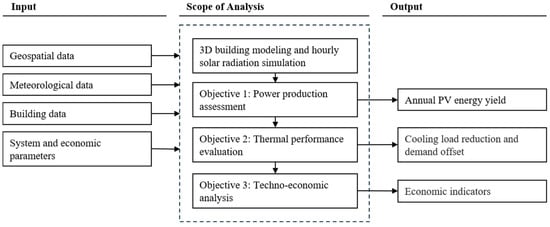
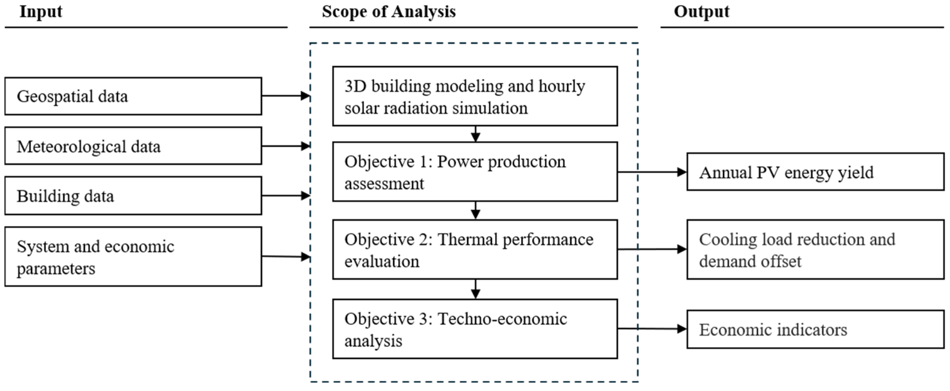
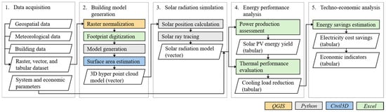
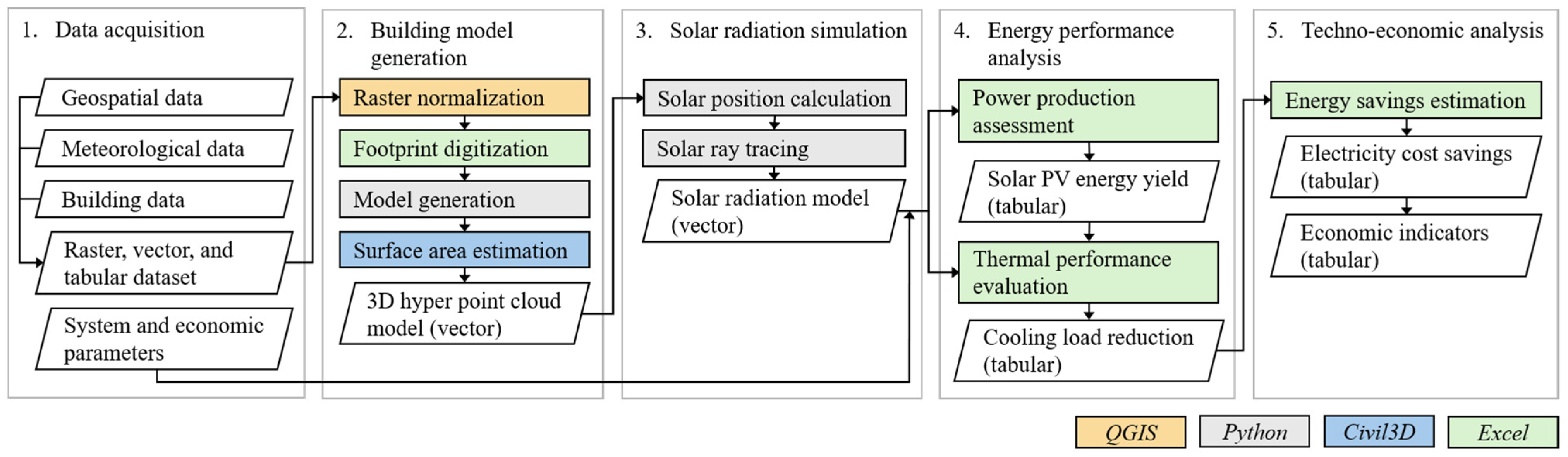
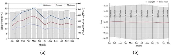
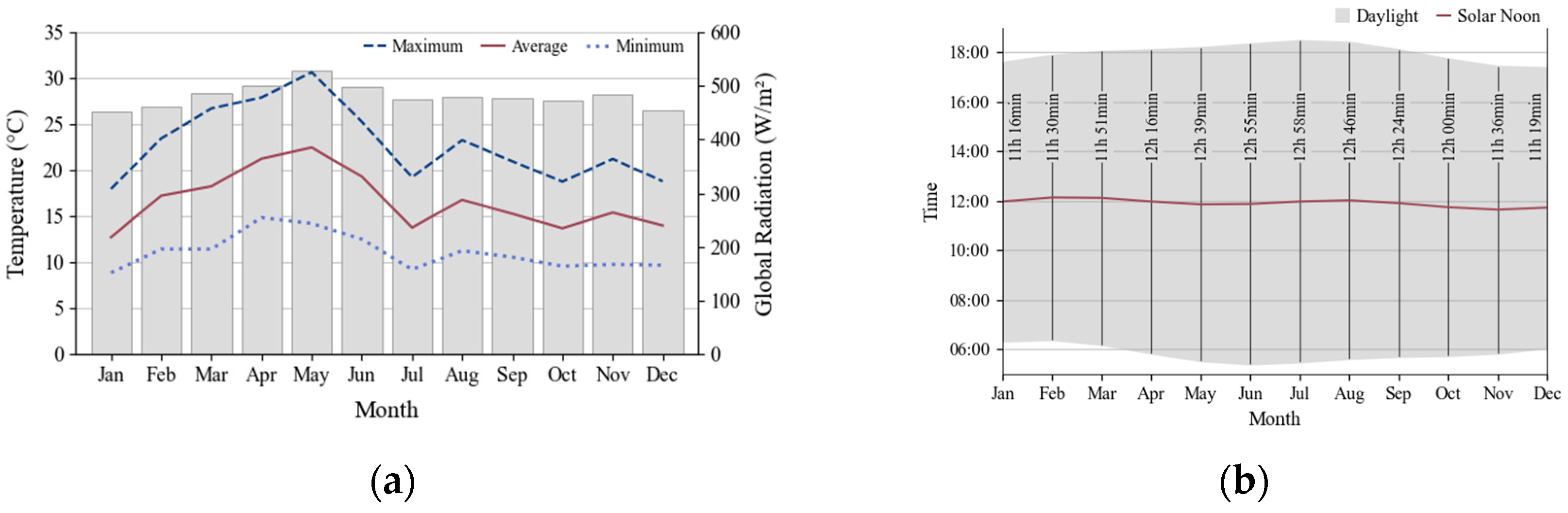
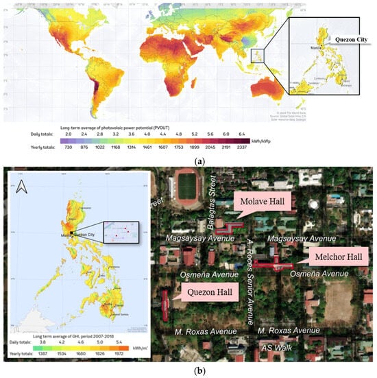
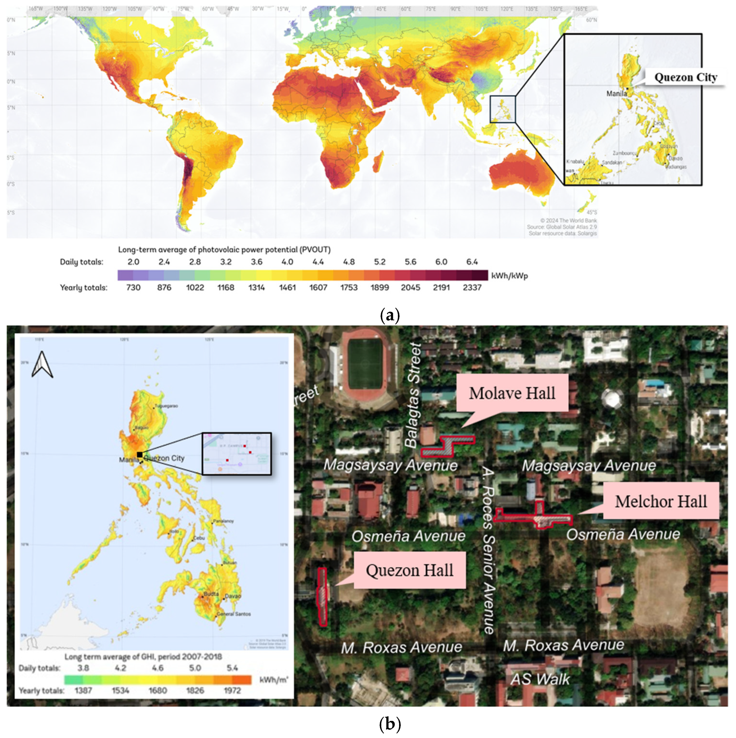
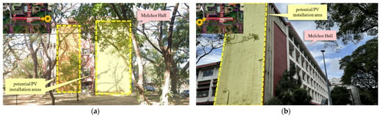
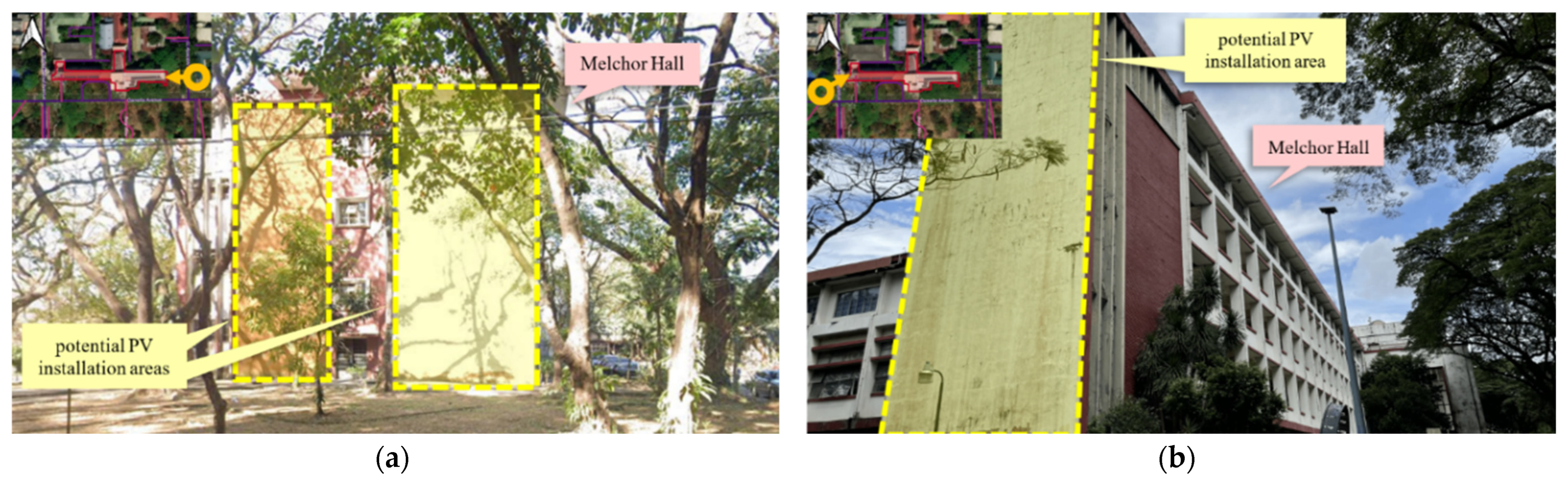
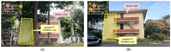
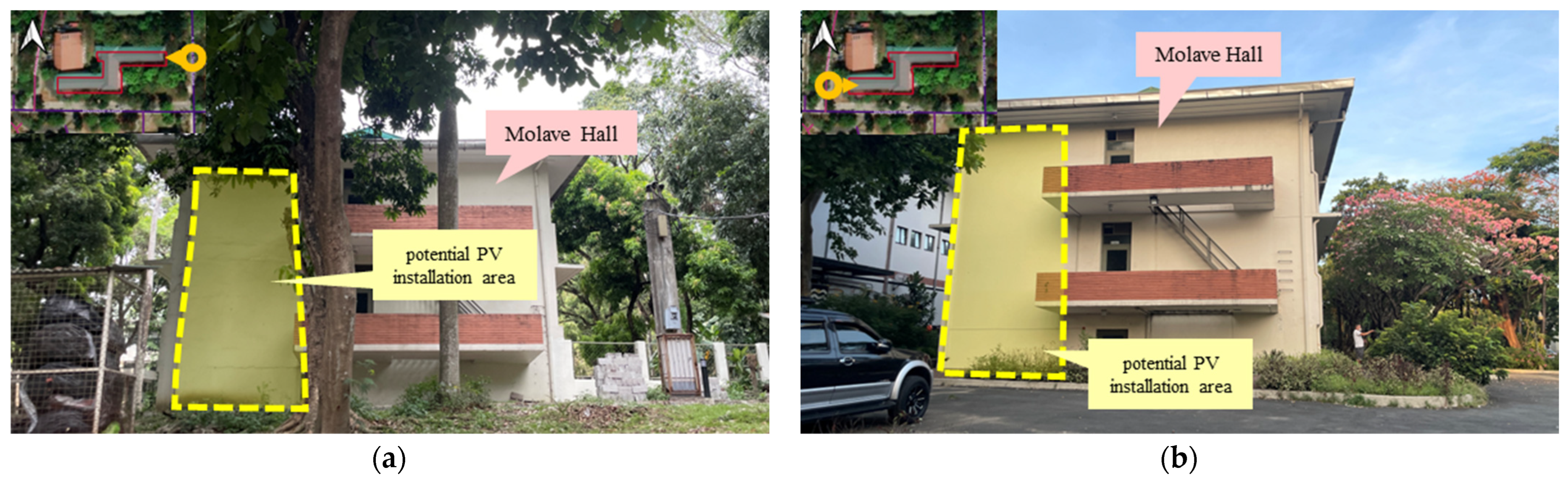
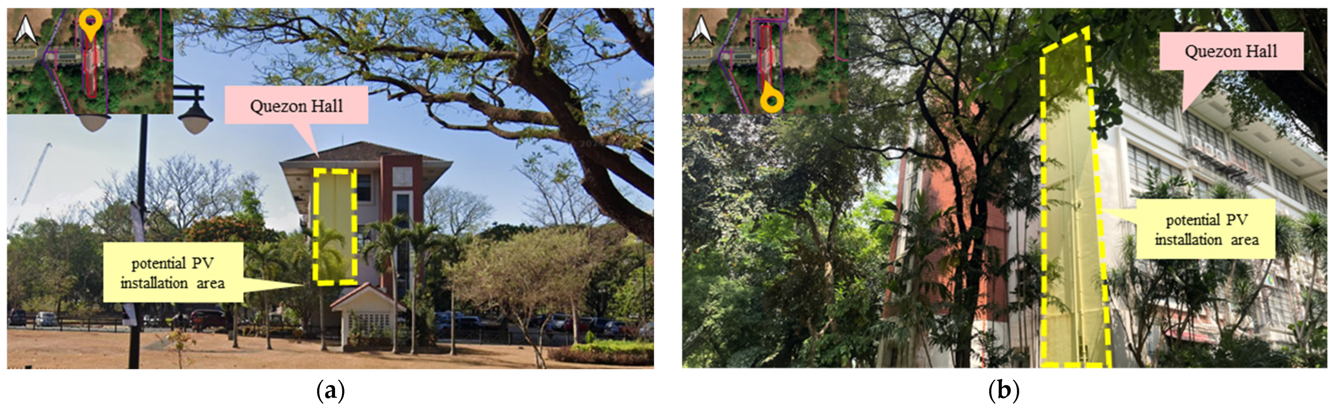
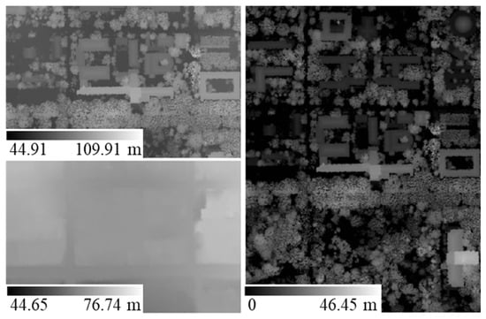
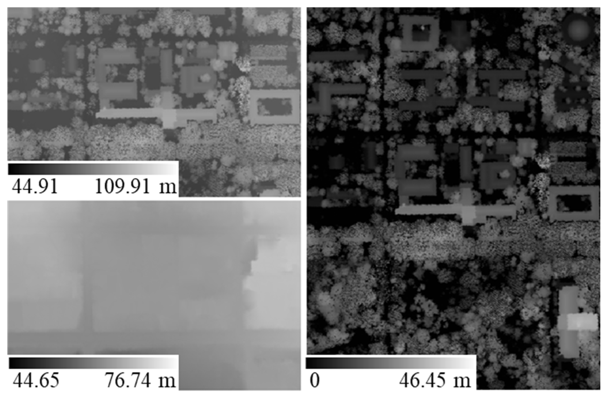


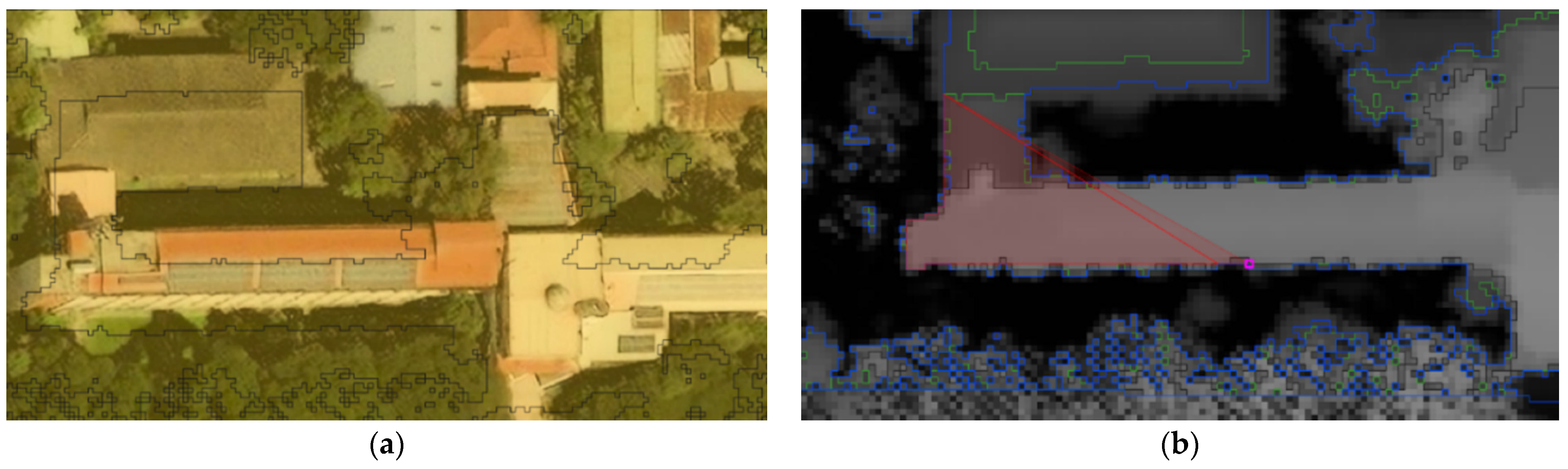
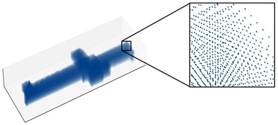
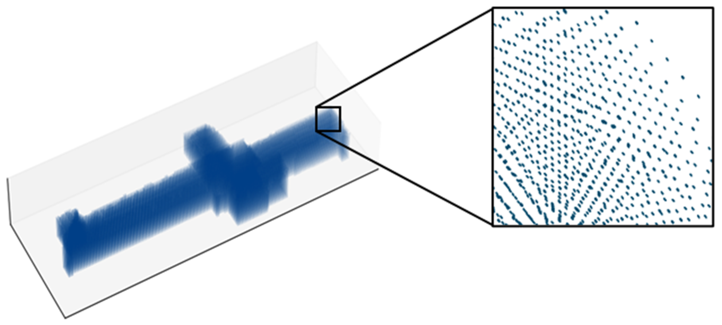
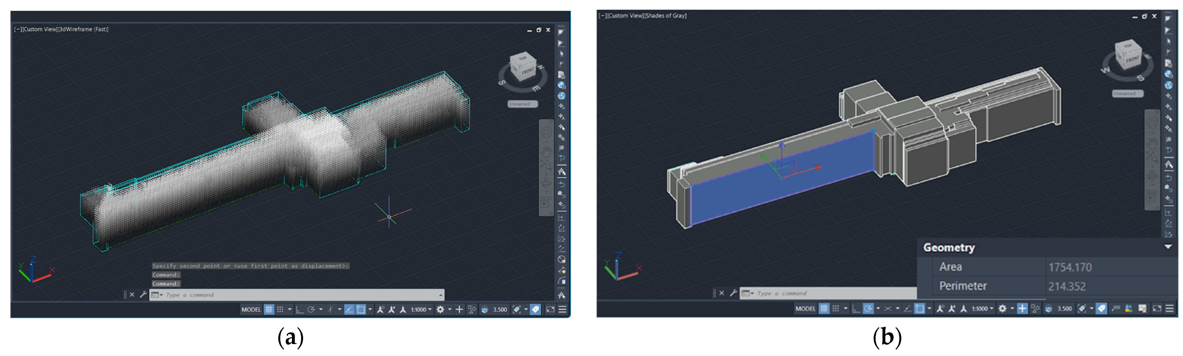
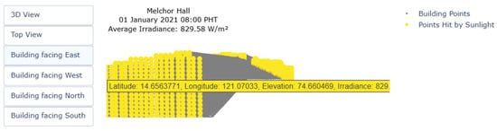
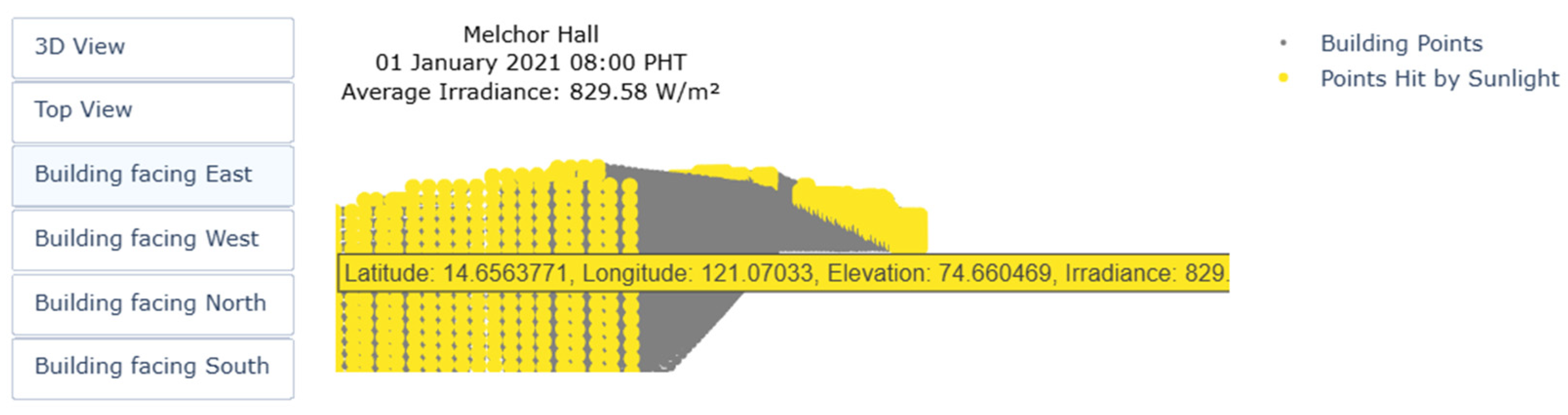
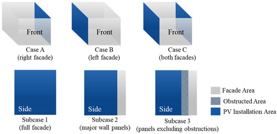
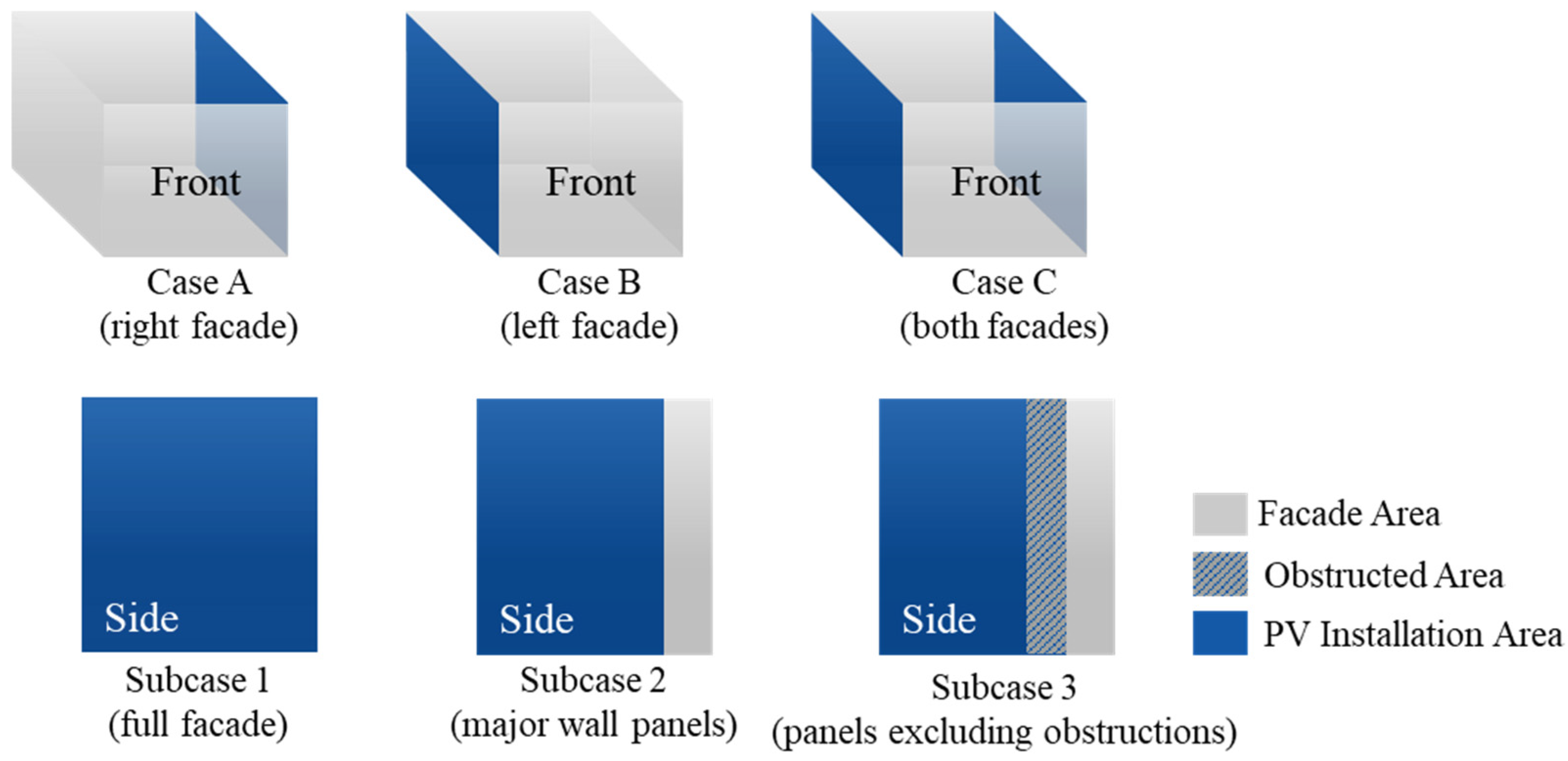
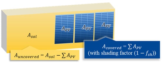
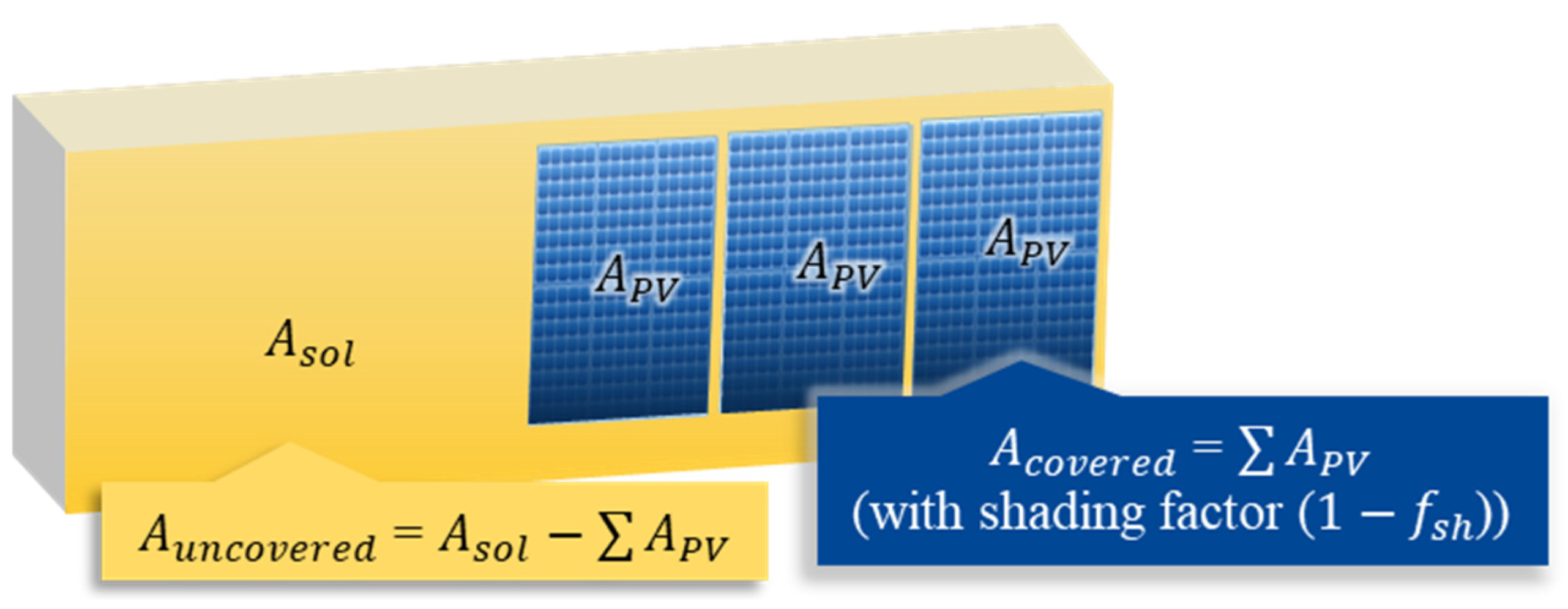
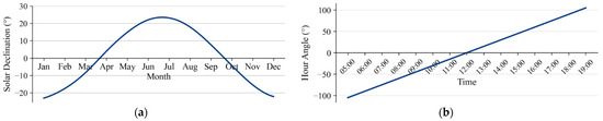
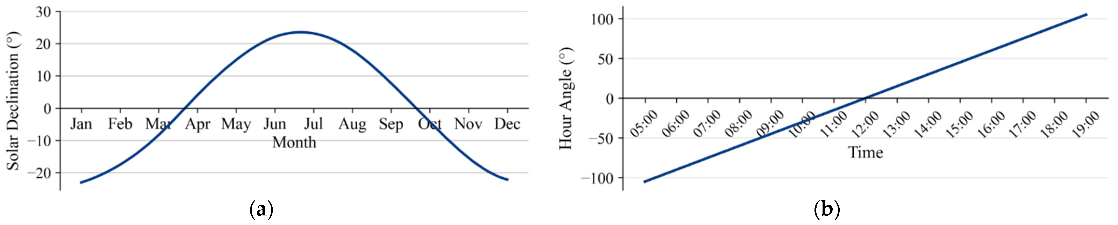
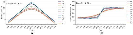
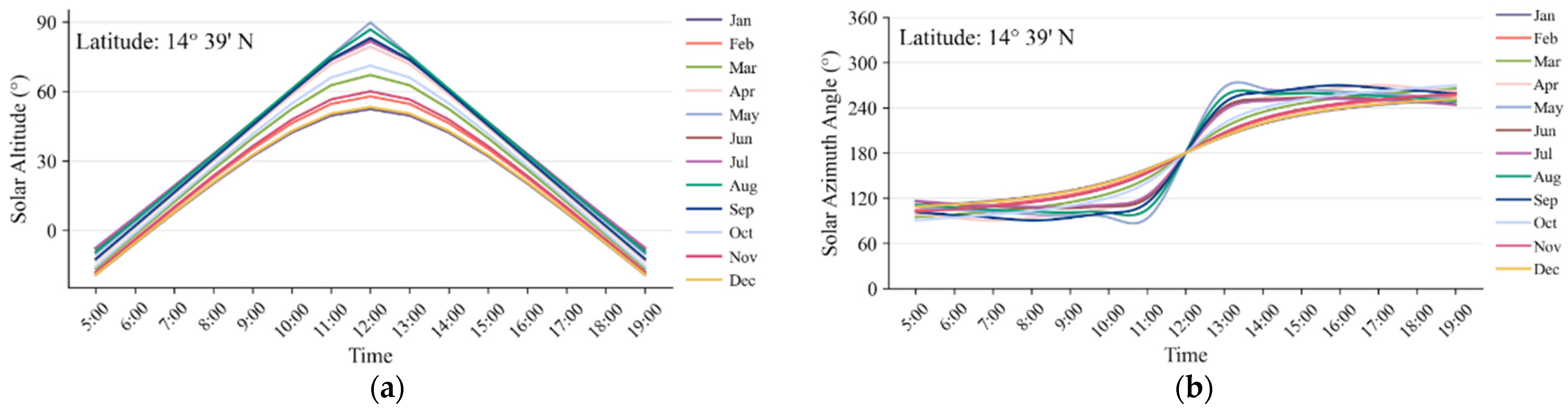
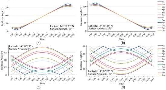
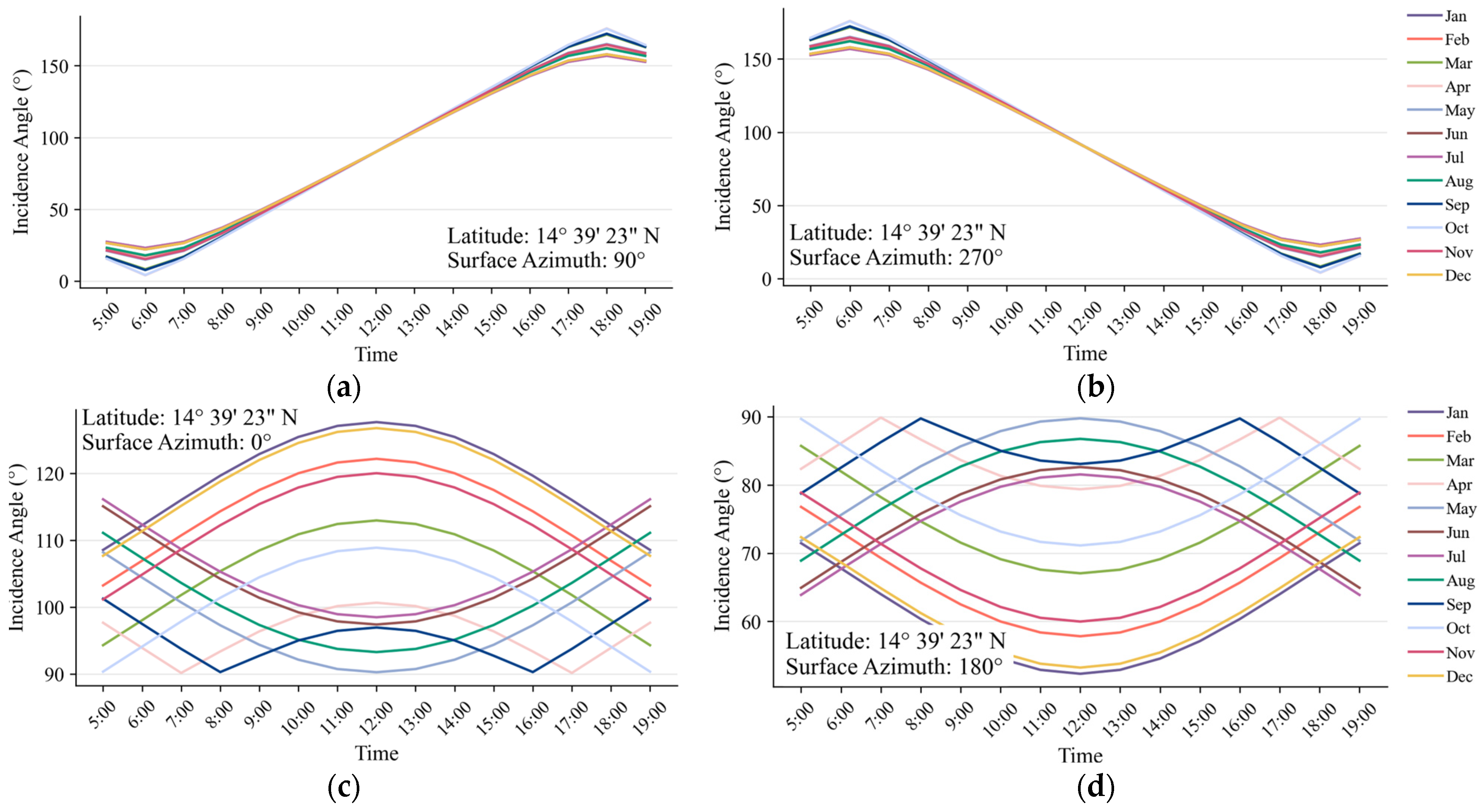
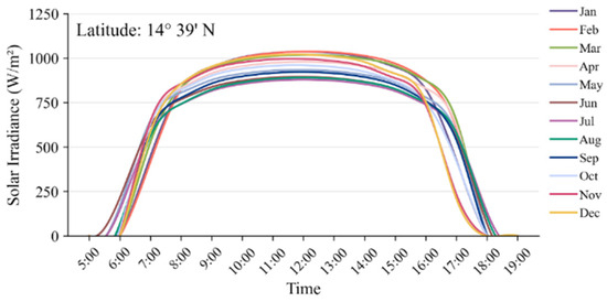
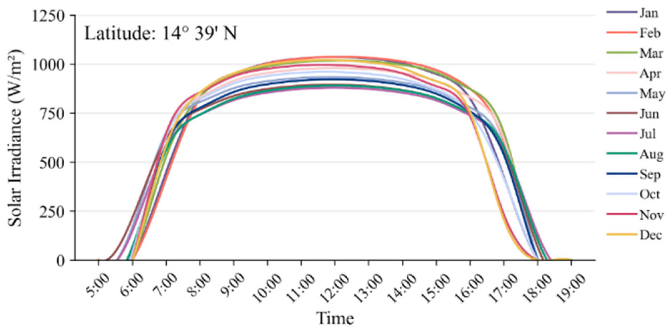
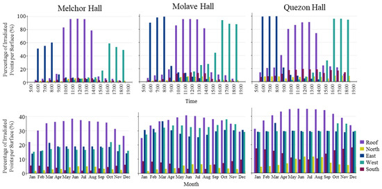
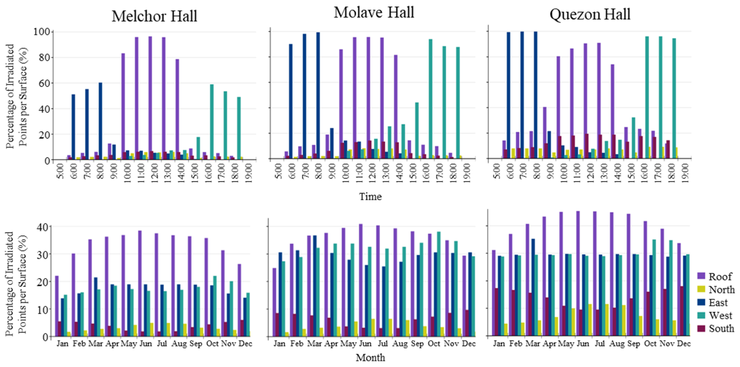
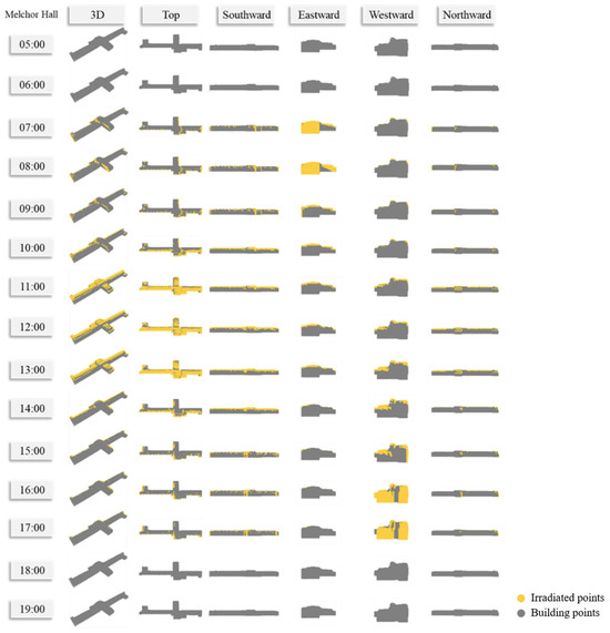
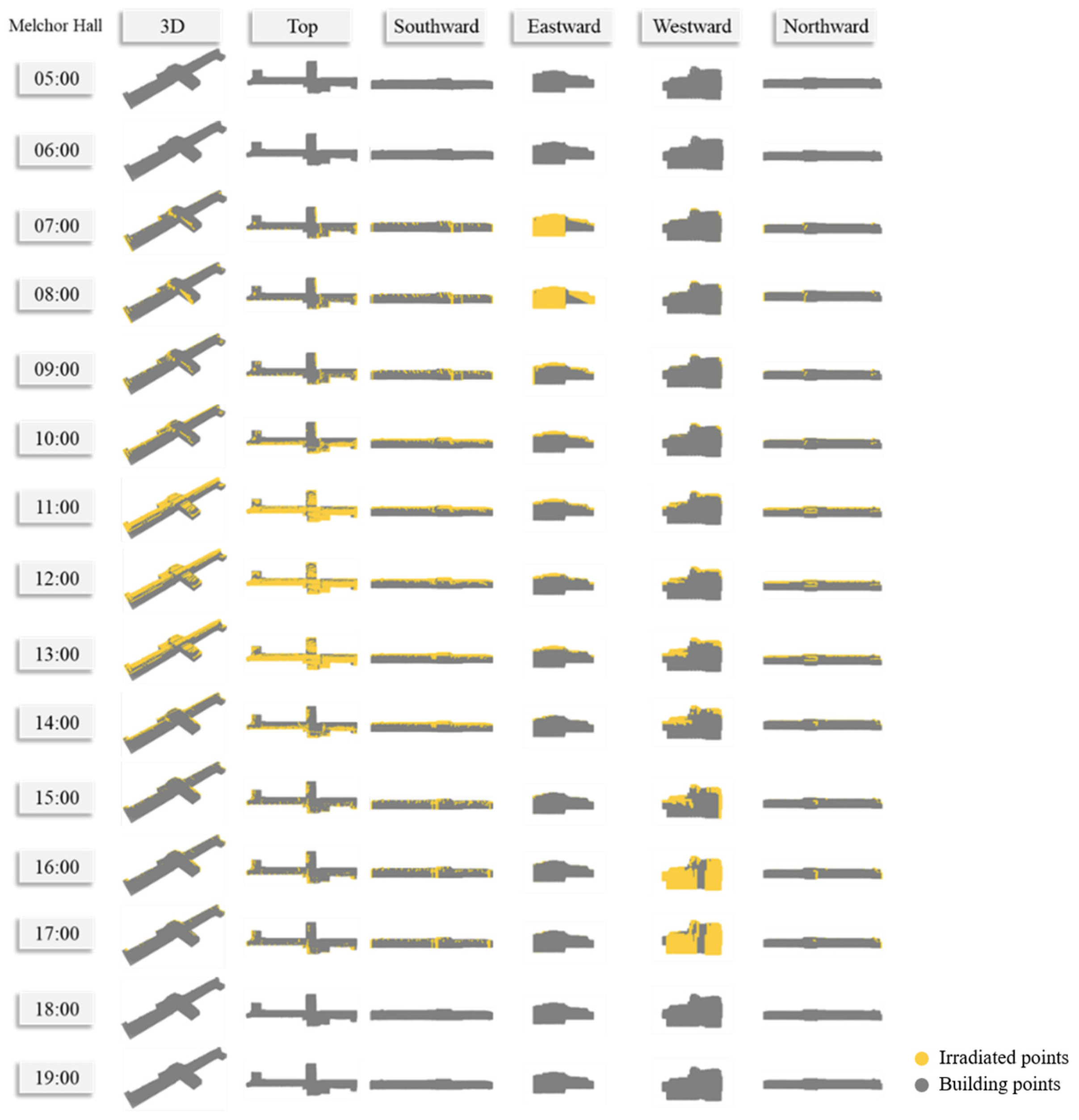
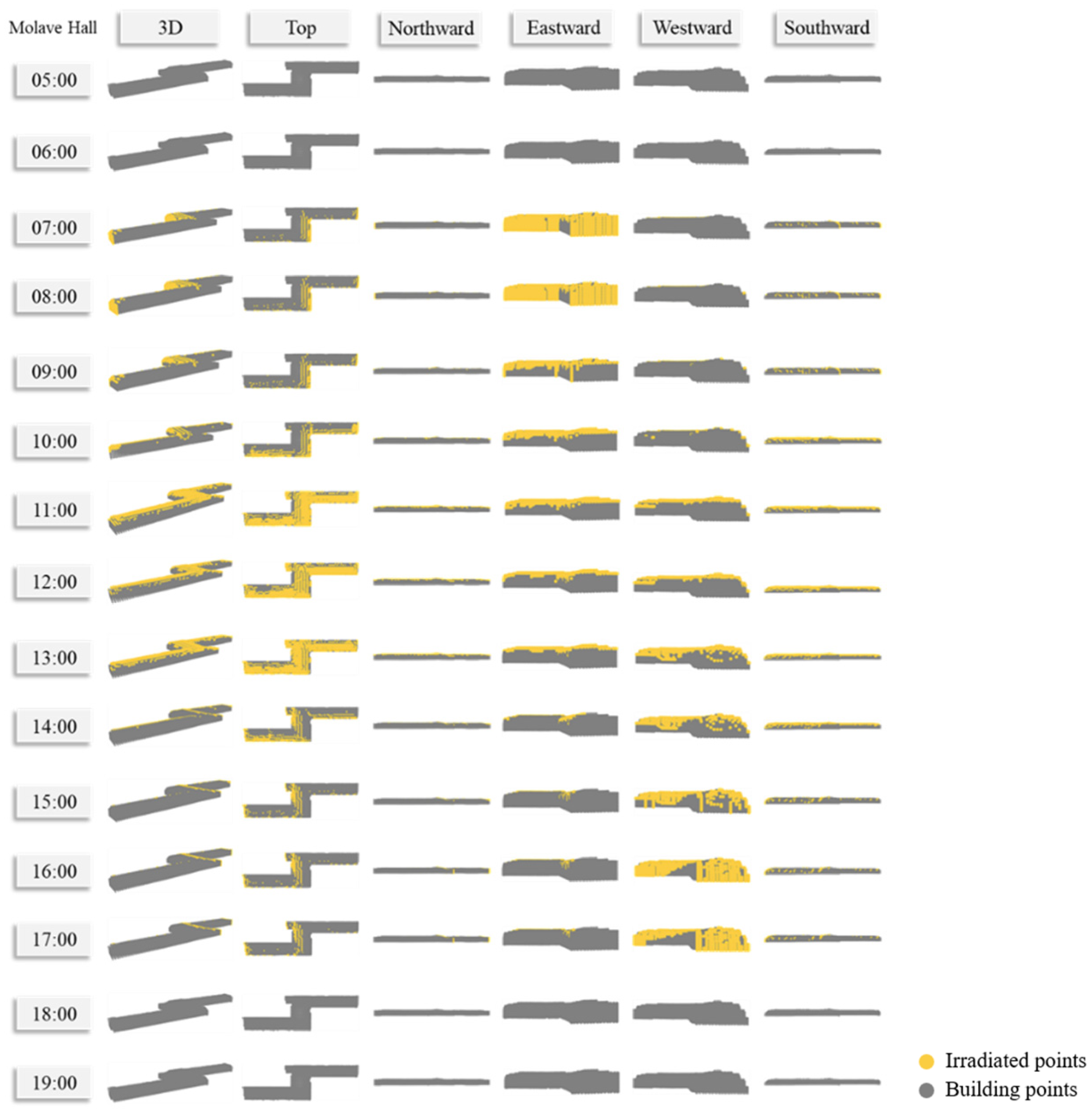
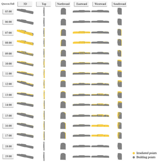
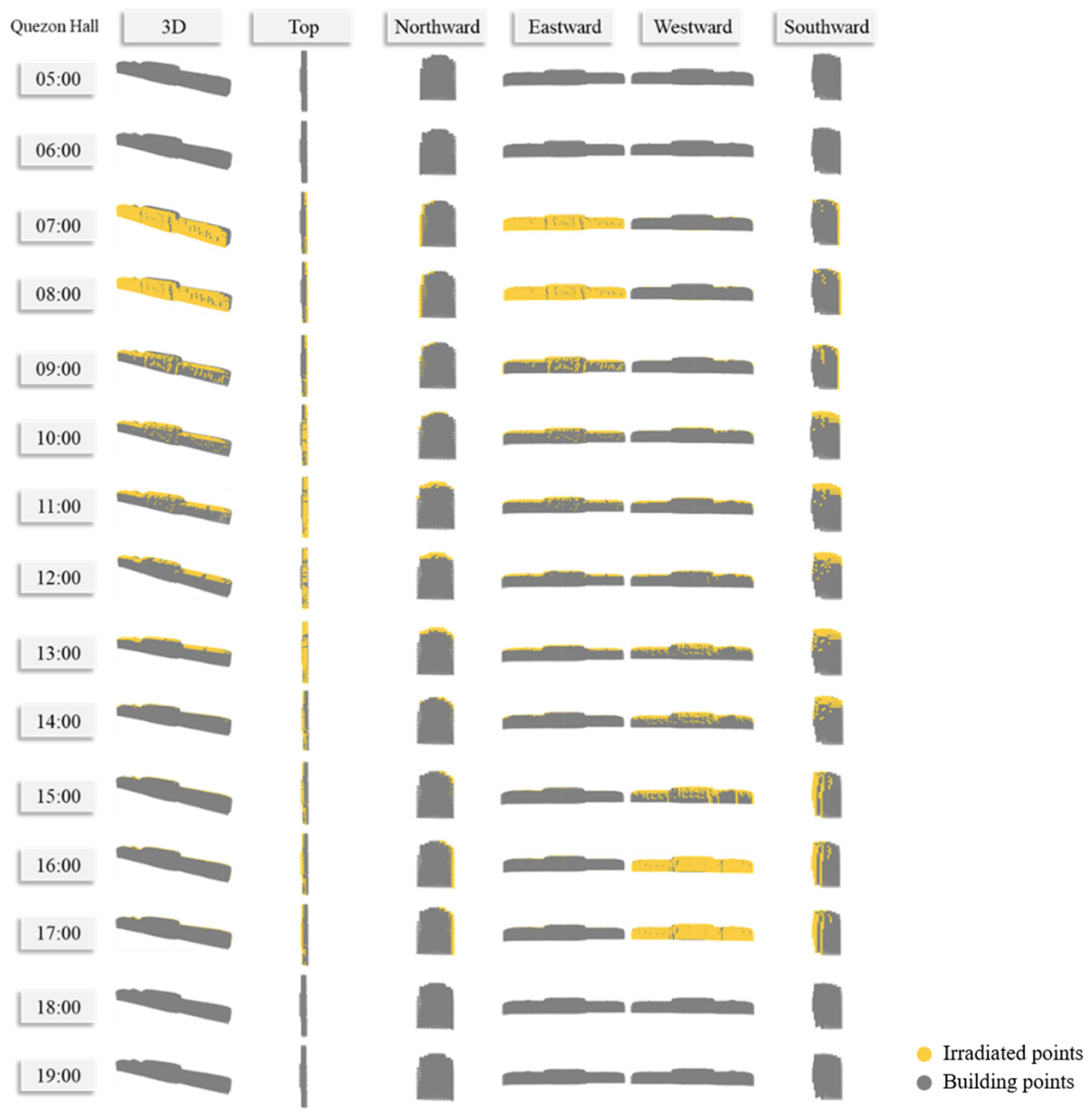
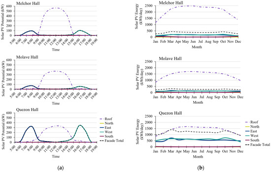
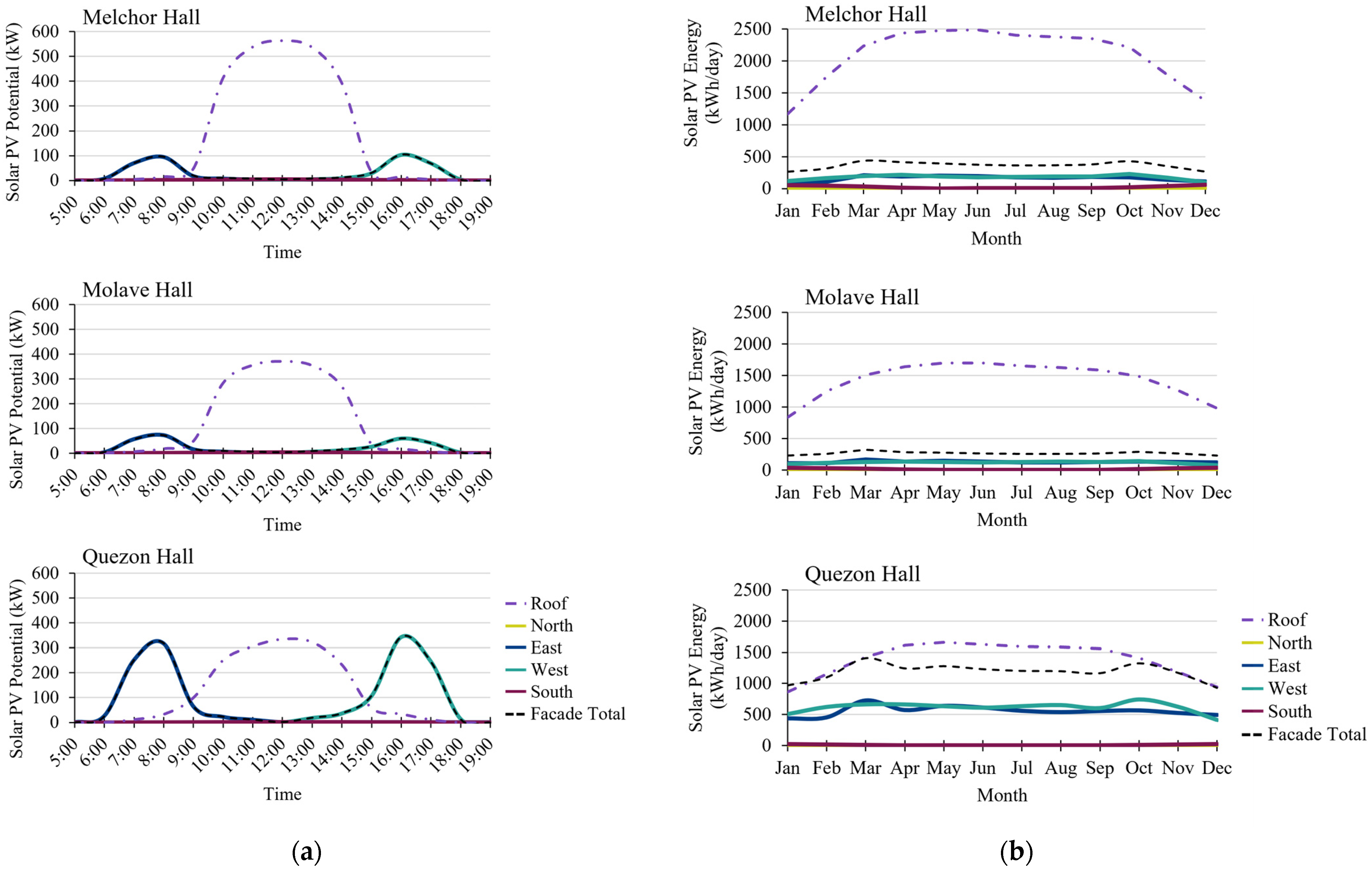
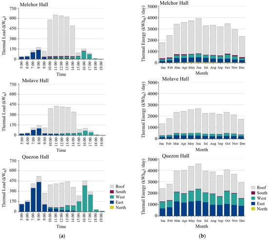
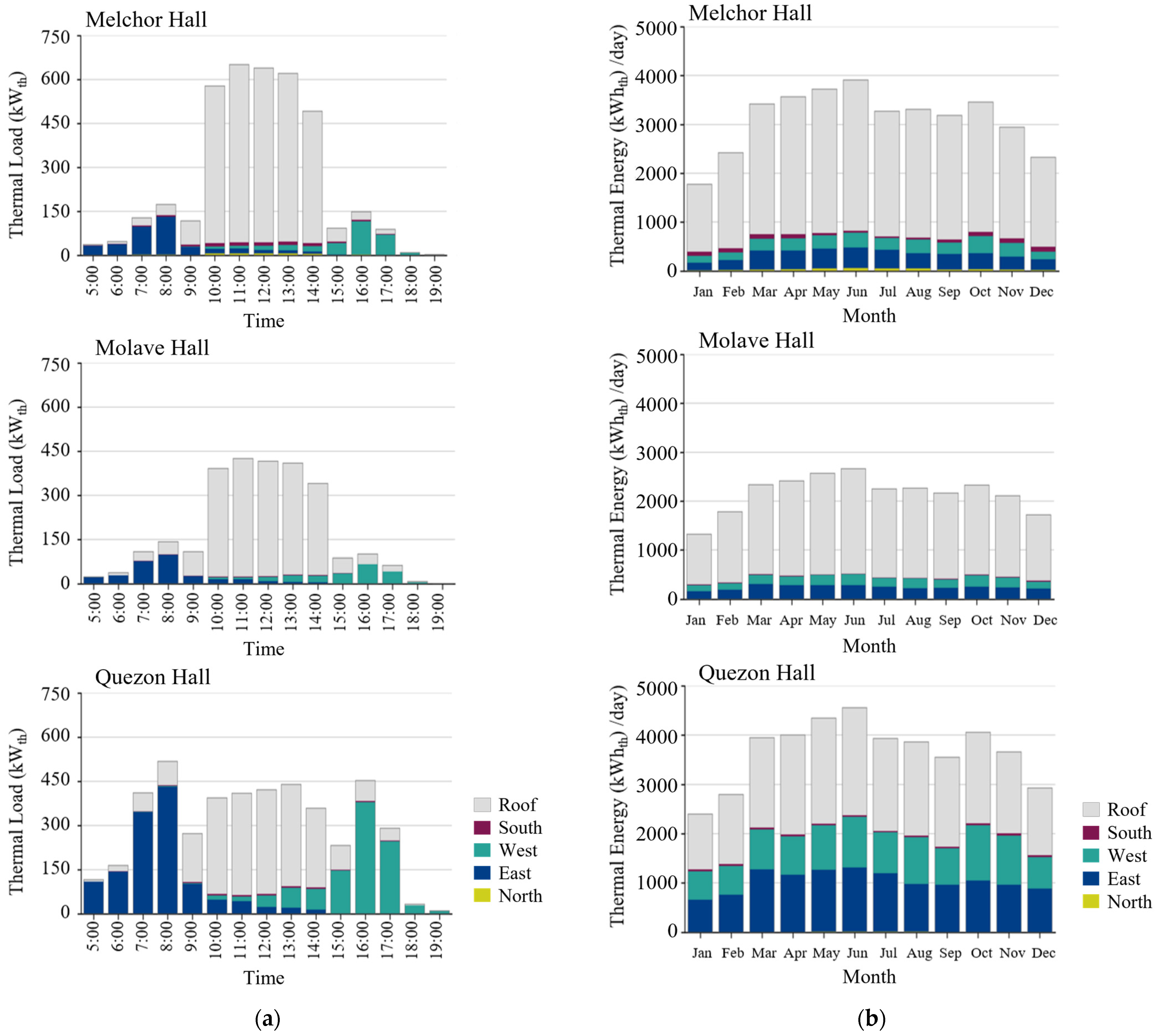
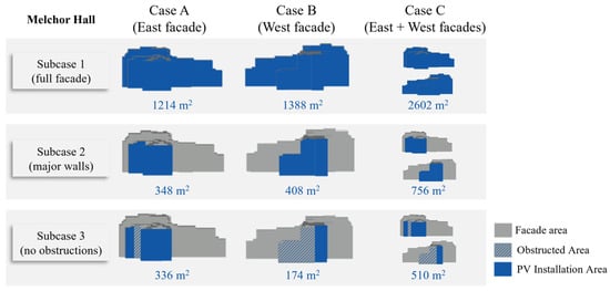
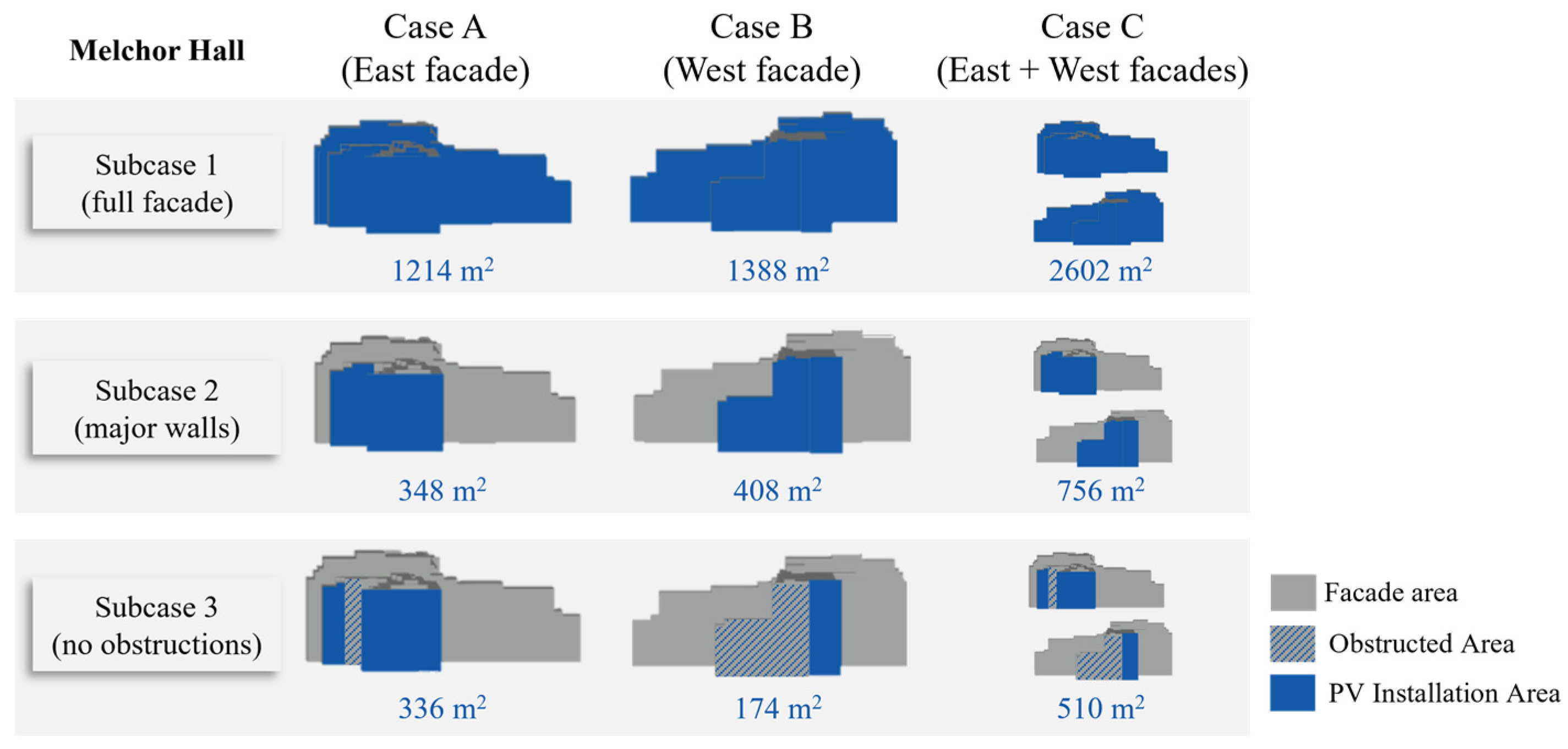
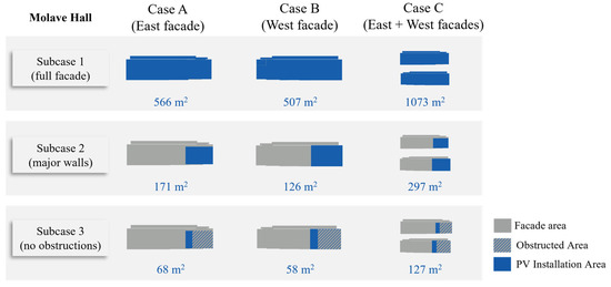
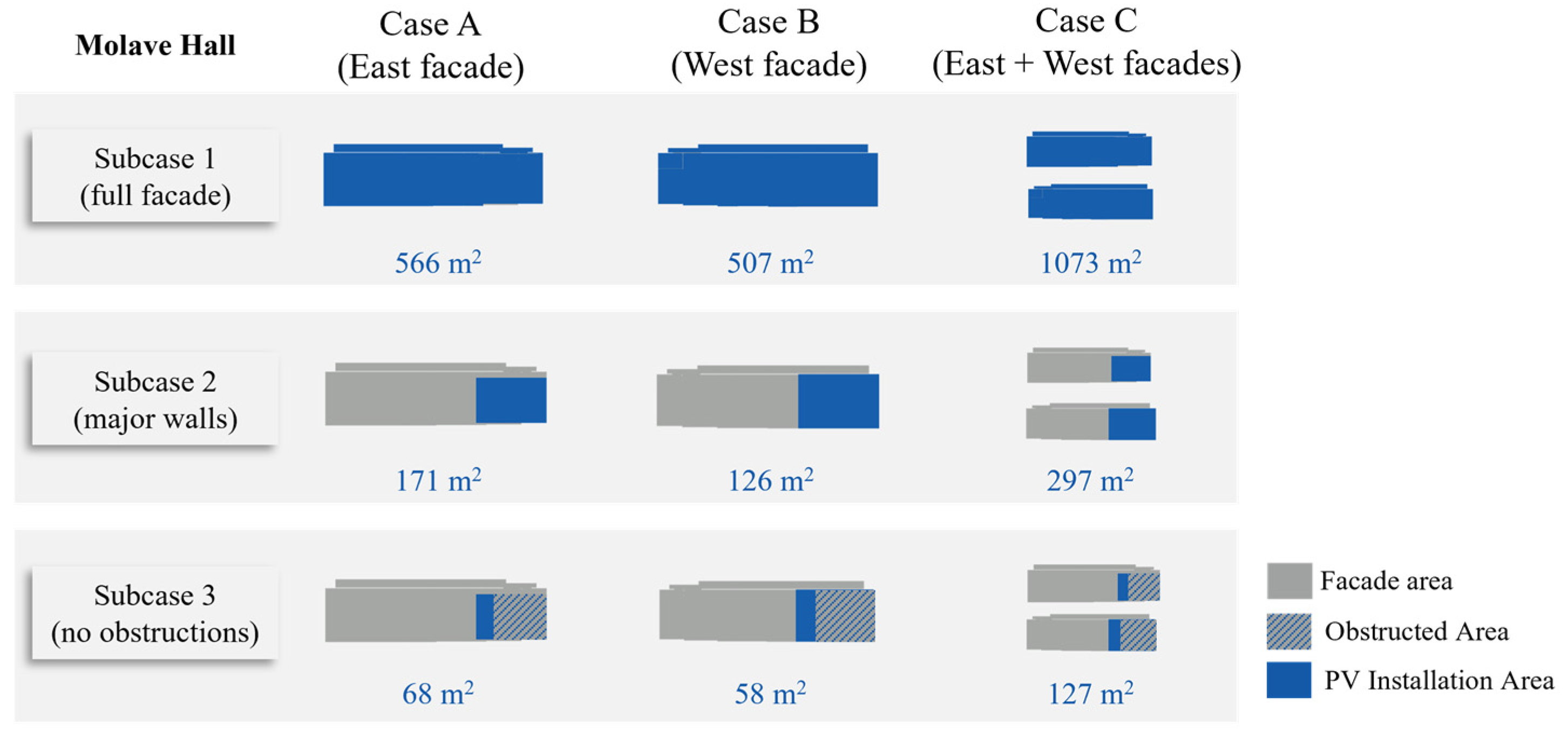
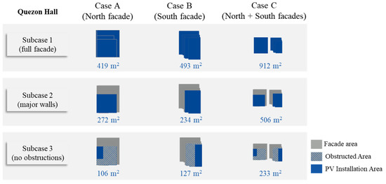
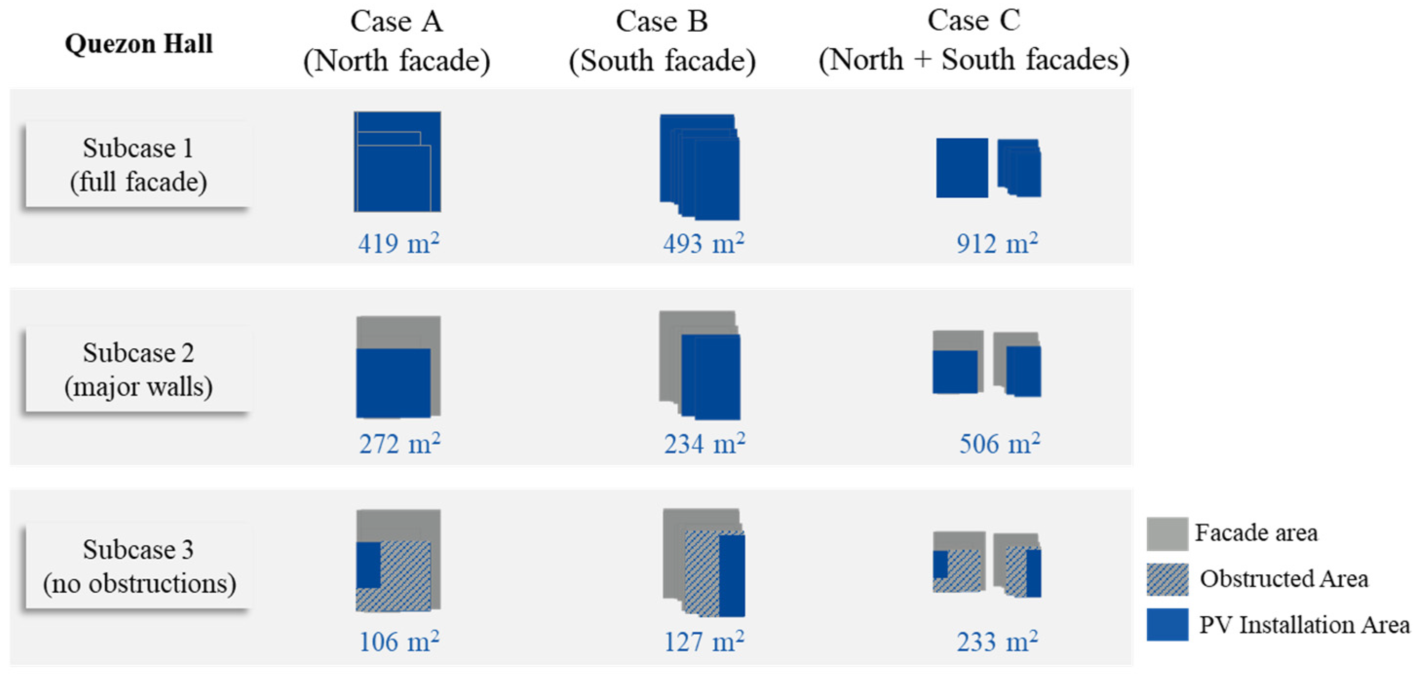
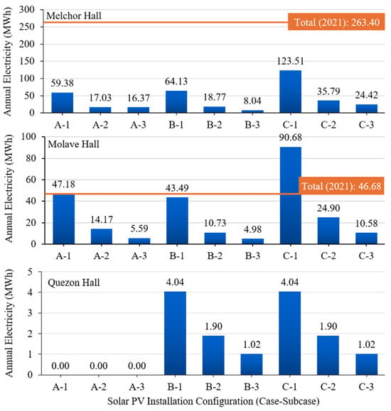
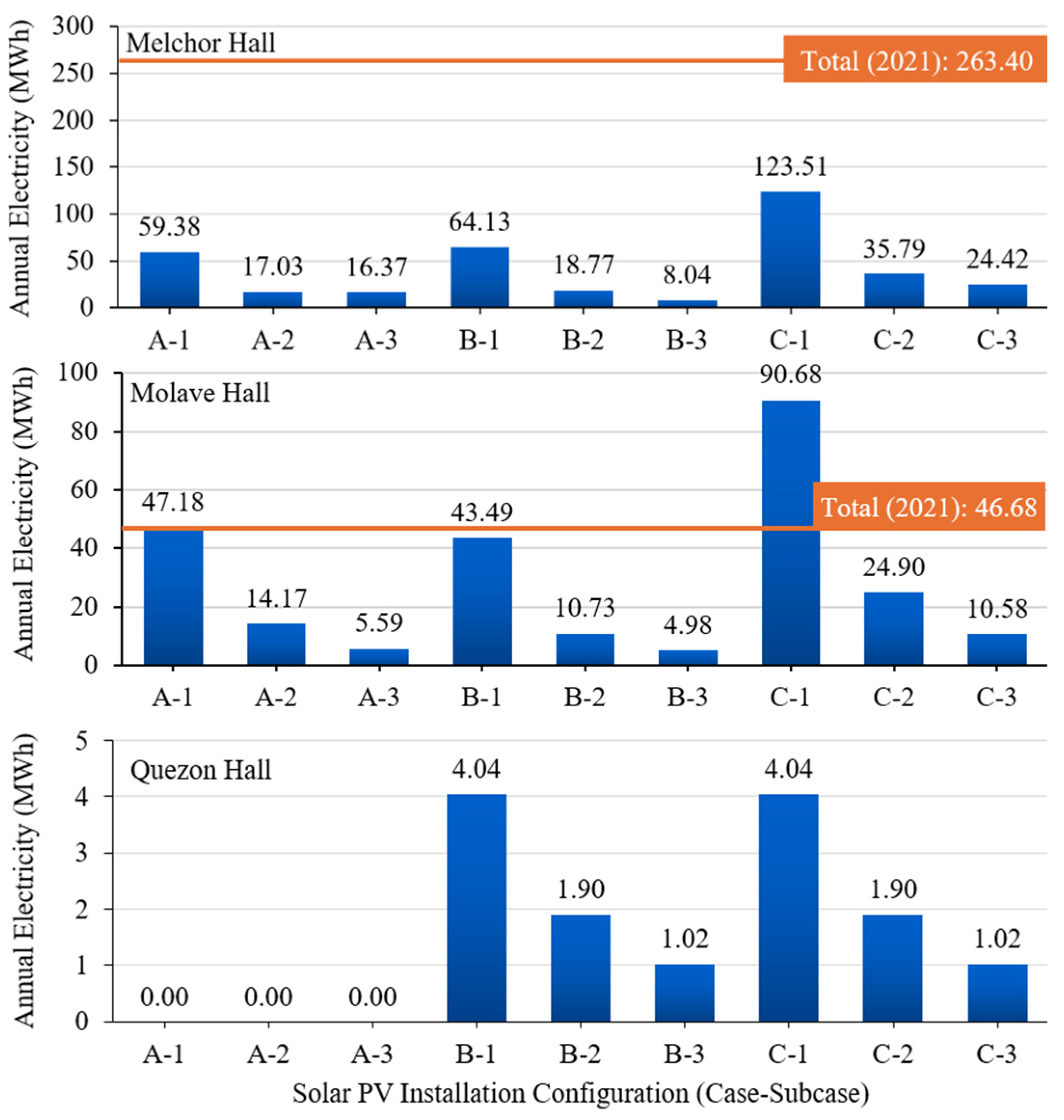
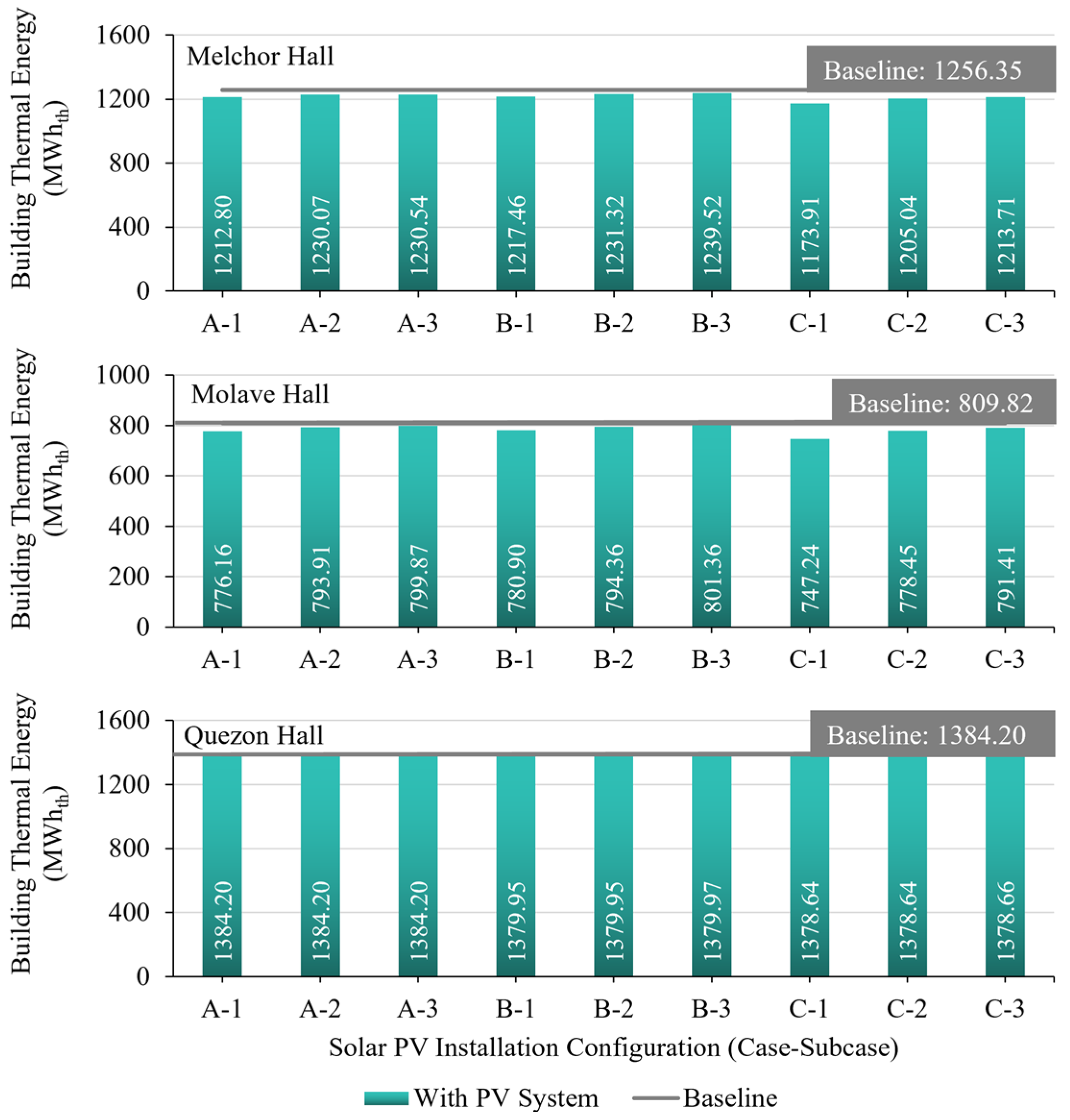
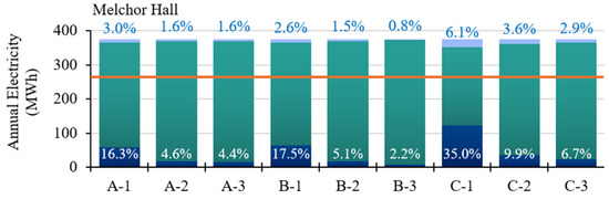
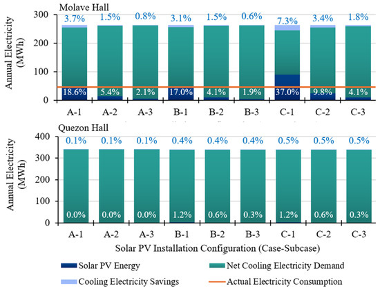
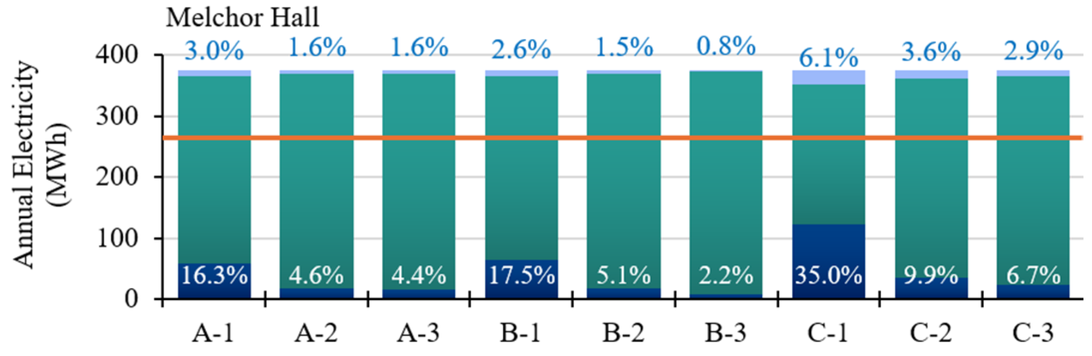
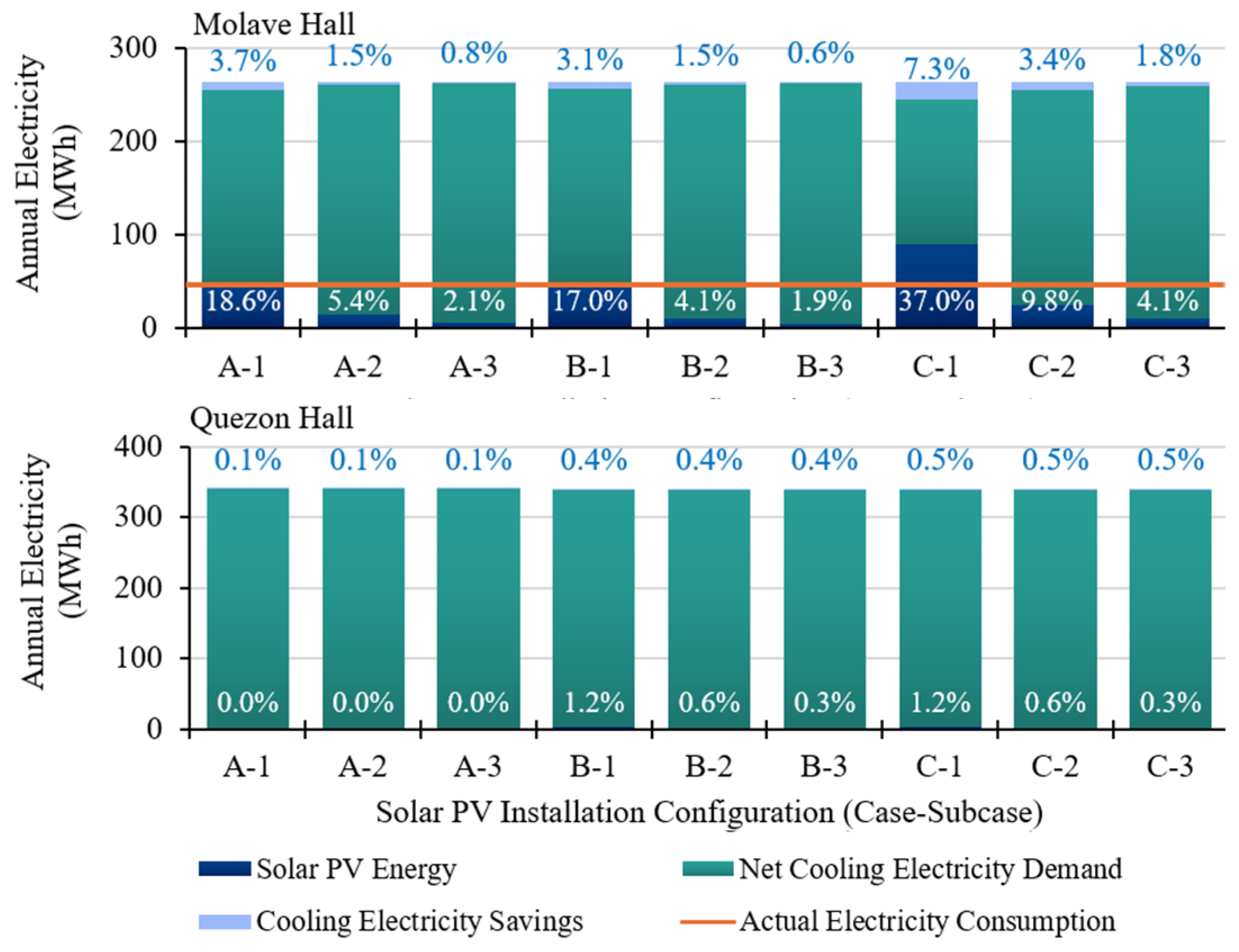
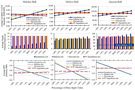
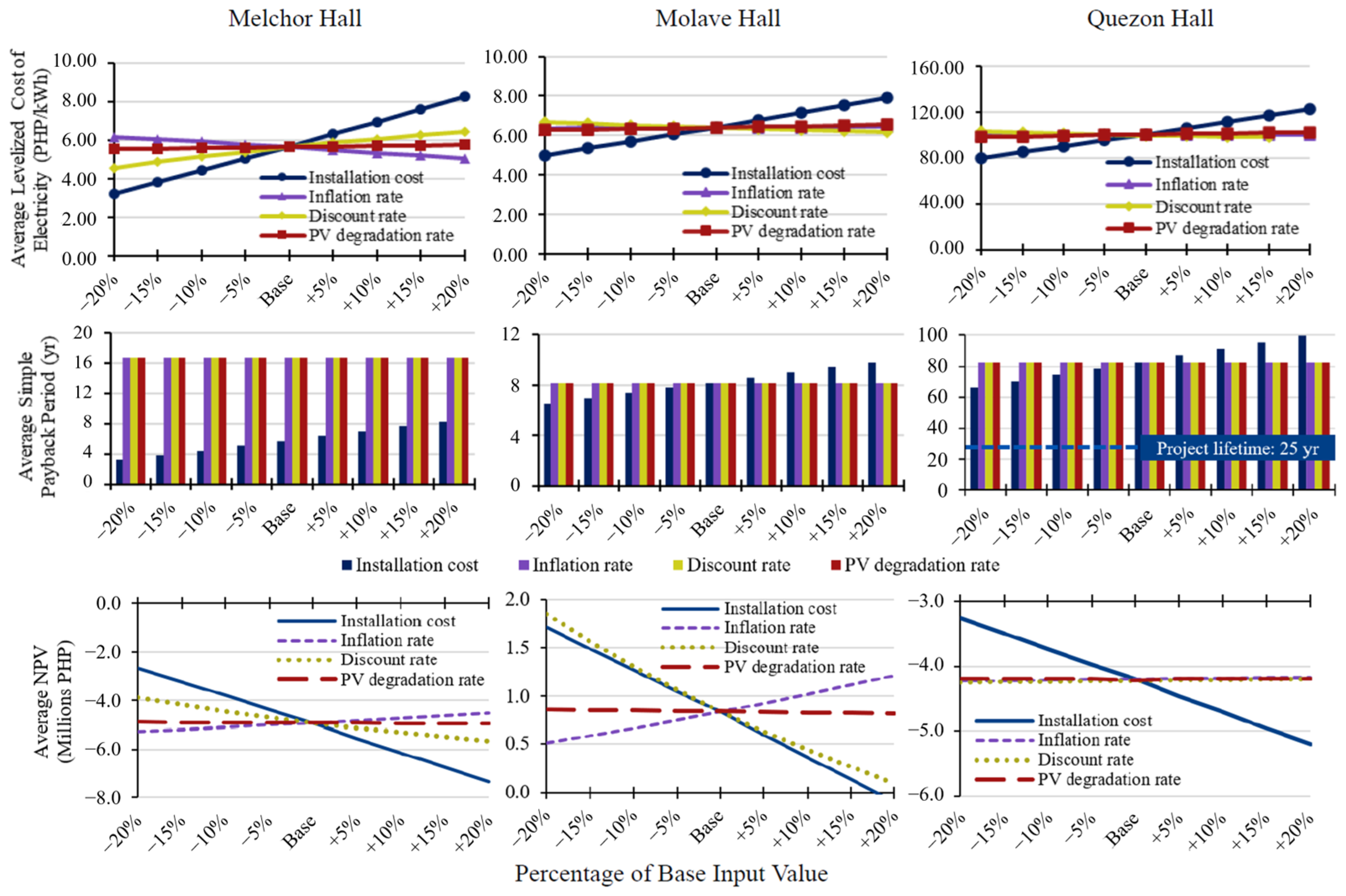

Disclaimer/Publisher’s Note: The statements, opinions and data contained in all publications are solely those of the individual author(s) and contributor(s) and not of MDPI and/or the editor(s). MDPI and/or the editor(s) disclaim responsibility for any injury to people or property resulting from any ideas, methods, instructions or products referred to in the content. |
© 2026 by the authors. Licensee MDPI, Basel, Switzerland. This article is an open access article distributed under the terms and conditions of the Creative Commons Attribution (CC BY) license.