


Abstract
In soft soil areas, cement–soil mixing piles are widely employed as a building foundation treatment measure, and their construction parameters directly influence pile uniformity and the stability of foundation reinforcement. However, visual and quantitative methods to verify on-site improvement effects are currently lacking. This study aimed to improve the mixing uniformity between jet media and soil layers and proposed a quantitative evaluation method based on numerical simulation and image recognition. Taking the silty soil in the Nansha area in Guangdong Province, China, as the research object, combined with flow tests and discrete element simulations, an experimental simulation based on a linear model of adhesive rolling resistance was established. First, the entire process of the wet water spraying soil mixing method and visualizing particle behavior was simulated. Based on the Danckwerts mixing index, image recognition technology was applied to quantify the uniformity of cement–soil mixing at different rotational speeds. The simulation results revealed that increasing the rotational speed within a certain range (0–100 r/min) significantly improved the uniformity of cement–soil mixing by 33.3%. However, increasing the rotational speed still further (100–200 r/min) resulted in only a 15.8% improvement. Furthermore, excessive rotational speed caused a significant loss of cement within the designed diameter of the pile. Second, based on the cement retention rate inside the pile, a speed balance range suitable for the working conditions of this study was obtained. A good balance was achieved between the effective cement content inside the pile and the uniformity of cement–soil mixing, further ensuring the consolidation effect of the cement–soil pile.
1. Introduction
Soft soil is mainly composed of natural silt sediments with high water content, high compressibility, and low bearing capacity, as well as a small amount of humus. In the field of engineering, an increasing number of highways, railways, infrastructure, ports and other projects will inevitably pass through soft soil layers during the construction process. Consequently, it is necessary to improve the foundation [1,2] to enhance its stability, strength, bearing capacity, and other relevant properties. However, the diversity of causes, strong structural heterogeneity, and highly nonlinear mechanical behavior of the soft soil foundation means it has a complex engineering response mechanism that significantly increases the difficulty of foundation treatment and deformation control, presenting one of the main sources of safety risks in engineering construction [3,4].
Enhancing the strength of the foundation through cement–soil mixing piles is a common improvement measure [5,6] which aims to achieve high-quality mixing of cement and soil. The higher the uniformity of the two mixtures, the stronger the resultant mixing piles [7]. Nevertheless, certain problems arise during construction, such as uneven mixing between the spraying medium (cement slurry or different curing agent materials) and the soil layer, and the slurry is prone to phenomena such as joint filling and aggregation. After hardening, the strength of the pile body is uneven; consequently, the strength at the center of the pile is considerably higher than that at the edge of the pile. To resolve this, multiple researchers have improved the mixing uniformity between the spraying medium and the soil layer by modifying the drill bit [8], enhancing the construction process [9], changing the cement dosage [10], altering the position of the cement nozzle, adding curing agents [11,12,13], adding drag reducing agents, and other methods [14]. However, the inability to visualize the internal conditions of the foundation during the construction process, as well as the lack of optimization mechanisms and theoretical support, makes it difficult to design and control the formation of the improved body. Traditional strength evaluation relies on unconfined compression tests which are not only time-consuming and labor-intensive but also destructive [15], increasing unnecessary workload and trial and error costs [16].
If the mixing process of the foundation can be simulated through computer modeling, and the actual improvement effect of the foundation can be predicted, a more efficient and scientific foundation improvement method can be created [16]. However, differences may exist between the foundation improvement process simulated by computers and the actual implementation process on site. Therefore, when conducting foundation modeling and simulating internal conditions, greater consideration needs to be given to the actual situation. Currently, object modeling analysis can assume that it is a continuum or a non-continuum. Because the foundation belongs to a non-continuum, this study adopted an analysis method that assumes the object is a non-continuum: the discrete element method (DEM). DEM is a numerical analysis method [17,18,19] capable of calculating phenomena that cannot be tracked by continuum analysis techniques, such as detachment, sliding, and contact between elements. It can also predict particle motion behavior [20,21] and obtain particle-related force conditions [22,23]. Ucgul et al. [24] used discrete element simulation software to simulate the soil tillage process and design the parameters of tillage components. Wilson et al. [25] investigated the rolling behavior of dry particles by approximating rough surfaces with arrays of spheres and validating an analytical torque-based model against DEM simulations, which revealed that adhesion consistently increases rolling resistance. Wu et al. [26] developed an adhesion model for rolling contact, demonstrating that tensile stress induces crack blunting. This causes discontinuous crack propagation in hyperelastic wheels, with a novel stick–peel feature analogous to the stick–slip of sliding friction. Boschi et al. [27] investigated the micromechanical behavior of soils during grouting and jet grouting using a DEM framework. Nazari et al. [28] modeled a rigid cylinder rolling on an inclined rubber plane using a numerical boundary element solution with a standard linear solid. Through uniaxial compression tests and unconfined compressive strength tests, Wu et al. [29] established a discrete element simulation model based on the Edinburgh Elastic Plastic Adhesive (EEPA) contact model and calibrated the parameters of sand and clay. Zhou et al. [30] studied sandy soils with three different moisture contents and selected the EEPA model as the soil particle contact model to calibrate the relevant parameters. Overall, significant progress has been made in particle contact models, DEM-based calibration of wet cohesive particles, and numerical simulations of liquid–solid two-phase systems. However, most existing studies focus on specific sub-problems, and a holistic reproduction of actual construction sequences, calibration of material-specific parameters, and quantitative verification of uniformity remain relatively lacking. This is especially true for silty soil systems, where empirical parameters established for other soil types cannot be directly applied. Therefore, it is essential to develop an integrated experimental–simulation–quantification methodology for engineering parameter analysis.
To resolve the aforesaid problems, this study used the silty soil in the Nansha area in Guangdong Province, China, as the research object and combined flow tests and DEM simulations to calibrate the parameters of cement slurry, silty soil, and cement–soil slurry, providing a reference for the constitutive model. Using the DEM to simulate the mixing process at different speeds, the internal visualization of the foundation was achieved through the PFC 3D6.0 platform. The results were output as images and imported into the MATLAB R2024a analysis module to quantitatively analyze the uniformity of water and soil mixing at various speeds. Combined with the cement retention rate in the pile, the influence of speed on mixing uniformity was systematically revealed, providing theoretical and data support for the optimization of mixing speed.
2. Discrete Element Method Analysis
The DEM—proposed by Peter A. Cundall [31]—is an analysis method based on a discontinuous model. It views the research object as a collection of tiny particles and reveals overall mechanical behavior and reactions by tracking the motion of individual particles [32,33]. Cundell and Stack initially introduced the DEM into the field of rock engineering [31]. Subsequently, the DEM was gradually applied in the field of geotechnical engineering. With the updates and iterations of various discrete element software and the construction of multiple contact models, the application scenarios for this method have become more extensive. Among these are several different versions of the commonly used particle contact models. Firstly, the Hertz Mindlin model describes the contact mechanics process between particles in a nonlinear spring damping form. This model can accurately reflect the elastic response of particles under stress but does not consider adhesion effects, making it more suitable for simulating rigid particle systems without adhesion. Secondly, the bonded particle model simulates the bonding and fracture between particles by introducing permanent or quasi-permanent bonding at the contact point. It is commonly used to study materials with significant cohesion such as rock, soil, or concrete. Thirdly, the rolling resistance linear model adds a rolling resistance component based on basic contact mechanics to constrain excessive rotation and slip between particles. This makes it suitable for studying systems that require consideration of particle orientation and stacking stability. Finally, the adhesive rolling resistance linear (arrlinear) model takes account of both rolling resistance and short-range adhesion effects. It simplifies the van der Waals force or liquid bridge interaction between particles into a linearized attraction term and introduces it into the framework of rolling resistance. Thus, it not only characterizes the basic mechanical behavior of non-adhesive systems but also reasonably describes powder systems with fine particle aggregation or liquid bridge effects. Therefore, this model has a strong fit with the particle mixing and stirring process that formed the focus of this study. First, rolling resistance can avoid excessive nonphysical slip of particles during the stirring process, maintaining the rationality of the structure and motion characteristics. Second, the adhesion component can capture the bonding, agglomeration, and flocculation phenomena of particles during the stirring process. Therefore, rather than simply determining the generality or inherent advantages of the model, the core reason for choosing the arrlinear model is the high match between its physical mechanism and the research object.
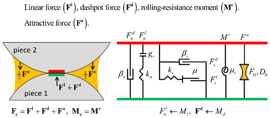
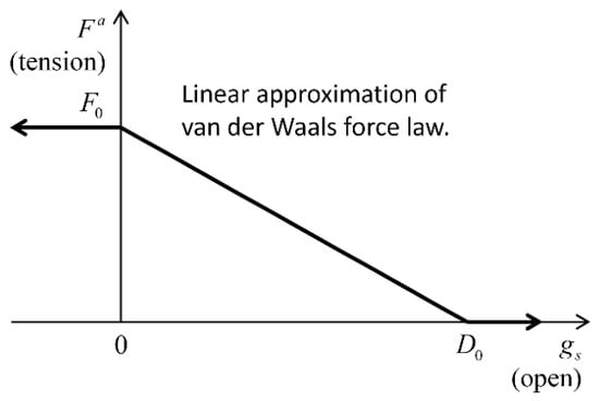
By adding a cohesive component to the rolling resistance linear model, the arrlinear model [34] characterizes the behavior of a cohesive granular material via a short-range attraction that serves as a linear approximation of the van der Waals force (Figure 1). The cohesive component is characterized by two parameters: the maximum attractive force (F0) and the attraction range (D0), as depicted in Figure 2. This displays the forces acting on piece 2 and the equal and opposite forces acting on piece 1.
Figure 1.
Behavior and rheological components of the adhesive rolling resistance linear model.
Figure 2.
Attractive force versus surface gap for the adhesive rolling resistance linear model.
3. Establishment of the Model
3.1. Engineering Background
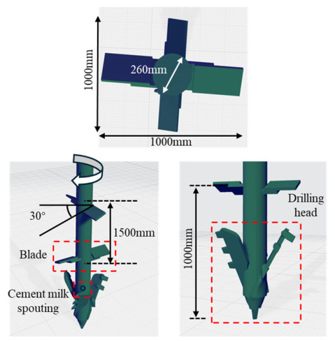
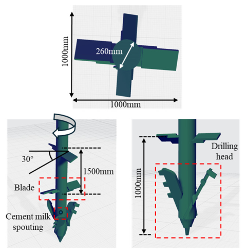
Ground improvement methods can have various effects on soft soil foundations, such as preventing liquefaction, improving bearing capacity, and promoting consolidation. At present, there are multiple methods for foundation improvement construction, such as the replacement method, accelerated consolidation method, compaction method, reinforcement method, and grouting method, which need to be selected and used according to the characteristics of the foundation [16]. The cement–soil mixing method is a type of consolidation technique which injects cement materials into the original foundation and mixes them with the in situ soil to achieve stable improvement of the foundation. This study examined the value of improving the uniformity of cement–soil mixing by changing the rotational speed in the wet water spraying soil mixing method. In this process, the top drilling tip is used to drill, and reserve holes at the edge of the drill rod behind the tip are utilized for synchronous spraying. The blades are used to mix the solidified material, as displayed in Figure 3. The three-dimensional mixing of foundation and solidification materials is then realized to form a homogeneous improvement body [35]. After quality testing and other verification, the foundation performance of the wet spraying cement–soil mixing method noticeably improves [36,37,38,39].
Figure 3.
Mixing component.
The experimental site was selected based on the principle of representativeness of geological strata in the Nansha area of Guangdong Province, combined with the existing site resources for investigation. According to nearby exploration and exposure, the strata from top to bottom were 0–2 m of miscellaneous filling soil layer, 2–18 m of silt layer, and 18–30 m of silty soil.
3.2. Contact Force Model
It was assumed that the analysis object was the on-site silty soil (with a depth of about 2–18 m); therefore, parameters needed to be set to reproduce the silty soil. A large body of research has been conducted on setting parameters for the discrete element method. Although various theories and formulas have been proposed, a clear setting method has not yet been determined. The parameter calibration method employed in this study was based on the work of relevant scholars [40,41,42]. This study used the flow test results of silty soil to determine parameters and aimed to make the model as simple as possible. This is because using complex particle contact models increases not only the computational costs but also the number of characterizing parameters, making it difficult to reasonably determine these parameters.
The contact force model used in this study is presented in Figure 1 and Figure 2. The adhesive rolling resistance linear model is based on the rolling resistance linear model, to which an adhesive component is added. It is a linear-based model that can be installed at both ball–ball and ball–facet contacts and is referred to in commands and FISH by the name arrlinear. Based on Gilabert [33,43], it describes simple cohesive granular materials. Cohesion is represented as a short-range linearized van der Waals attraction which, unlike PFC 3D6.0-bonded materials, does not break once surfaces come within the attraction range. Gilabert [33,43] found that cohesive grain assemblies can achieve stable, loose structures with solid fractions as low as 25–30%, compared with 58–64% for non-cohesive systems. Although cohesive materials are less studied numerically, this model applies to both cohesive and non-cohesive systems and can capture the macroscopic behavior of powders (e.g., xerographic toners) and wet bead packs, where cohesion arises from van der Waals forces or liquid bridges.
The force–displacement law for the adhesive rolling resistance linear model updates the contact force and moment as in Formula (1):
where FI is the linear force, Fd denotes the dashpot force, Fa represents the attractive force, and Mr is the rolling resistance moment. The linear force, dashpot force, and rolling resistance moment are updated in accordance with the rolling resistance linear model, while the attractive force is updated as follows.
The attractive force acts in the normal direction by Formula (2):
where is tension (attraction).
The attractive force (see Figure 2) is calculated using the following Equation (3):
where is the surface gap.
In addition to the energy partitions of the rolling resistance linear model, the adhesive rolling resistance linear model provides the following energy partition: adhesive energy, , defined as the work done by the attractive force on the contacting pieces. If energy tracking is activated, this energy partition is updated as follows by Formula (4):
where is the attractive force at the beginning of the timestep, and denotes the relative normal-displacement increment of this equation in the “Contact Resolution” Section. It is important to note that may be positive or negative, with the convention that the work done by the attractive force on the contacting pieces is positive.
3.3. Determination of Material Parameters
When using the contact force model described in Section 3.2 for analysis, the following material parameters need to be determined:
- (1)
- Young’s modulus—emod (Pa);
- (2)
- Stiffness ratio—kratio;
- (3)
- Friction coefficient—firc;
- (4)
- Normal critical damping ratio—dpnr;
- (5)
- Shear critical damping ratio—dpsr;
- (6)
- Dashpot mode—dpm;
- (7)
- Rolling resistance coefficient—rfric;
- (8)
- Maximum attractive force—F0 (N);
- (9)
- Attraction range—D0 (m).
This study referred to multiple previous studies on the DEM and attempted to simulate the target basis by setting the parameters. Density is determined by measuring specific gravity. Research has demonstrated that the damping coefficient is a key parameter determining the deformation rate of the specimen in slump tests [44]. When the damping coefficient is small, the deformation speed of the sample is fast, quickly reaching the final state. Conversely, when the damping coefficient is large, the deformation process is relatively slow. In addition, the damping coefficient has a relatively small impact on the final state of the flow [16]. In this study, three groups of samples completed flow within approximately 0.5–0.7 s; therefore, the damping coefficient was pre-set to 0.2 to meet a flow stop time of approximately 0.5 s, assuming that the normal and tangential damping coefficients were the same. To balance computational complexity and facilitate analysis, spherical elements are used in modeling. However, the contact between spherical particles is point contact, which makes it difficult to consider rolling resistance and can easily lead to excessive rotation of the particles. The introduction of a rolling resistance model can effectively suppress this phenomenon [45]. Previous studies have revealed that setting the rolling resistance coefficient to 0.05~0.30 can avoid excessive particle rotation [46]; hence, this study assumed it to be 0.1. According to research, a linear relationship exists between the friction coefficient and slump expansion [44], and it is speculated that this is also true in silty soil. If the friction coefficient can characterize viscosity, then fine-tuning its value means that the simulated flow results can be consistent with the experiment. Therefore, maximum attraction was set to 0–1 times the average weight (N) of a single particle, and the range of attraction was taken as 1.1 times the average particle radius R [40].
3.4. Particle Shape and Initial Conditions
To simplify modeling, this study idealized the particle swarm as a sphere. The filling method of non-equal diameter or non-spherical particles can significantly reduce simulation efficiency, and their complex arrangement may increase experimental data dispersion [47,48,49]. Research has shown that equal-diameter particles can also simulate the mechanical properties of materials [50], which has significance for analyzing soil fragmentation and deformation. Thus, this study used equal-diameter particles to simulate the mechanical behavior of soil samples.
4. Calibration of Target Soil Layer Parameters
4.1. Flow Test
To understand the flowability of silty soil, a stainless-steel test mold with a diameter of 30 mm and a height of 50 mm was used for flow testing [16]. The silt soil used in this experiment was the silt soil in the site, which had a natural moisture content of 45%, a density of 1.66 g/cm3, and a porosity of 50%, ranging from 2 to 18 m from top to bottom. Next, 42.5 Portland cement was selected and a cement slurry prepared with a water–cement ratio of 0.8:1. The stainless-steel test mold was then placed in a horizontal plane, following which the muddy soil was placed into the stainless-steel test mold by keeping it vertical, slowly lifting it up, and then pouring in the soil. After cleaning the plane and the test mold, the cement slurry was poured in. The cement soil was then prepared in proportion. To compare the flow behavior of the flow section based on the DEM with the flow test results, the flow value per unit time was obtained.
4.2. Experimental Reproduction
The set of DEM parameters for this analysis are presented in Table 1.
Table 1.
Set of DEM parameters.
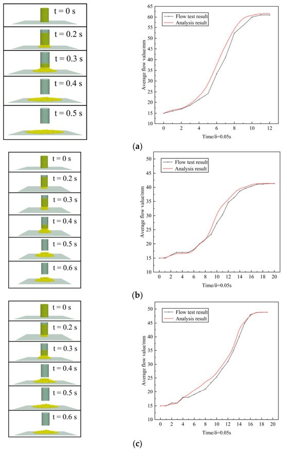
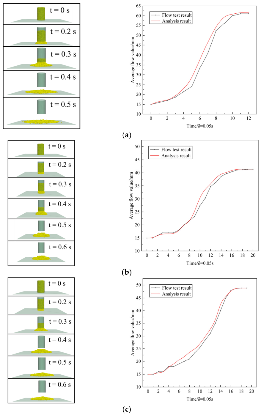
The corresponding parameters and conduct flow tests were then set to reproduce the cross-sectional changes in cement slurry, silty soil, and cement–soil slurry. Comparisons of the “flow behavior of discrete element method flow analysis” and “flow behavior of flow test” of the three groups of objects were then performed, as displayed in Figure 4.
Figure 4.
Comparison between discrete element flow and actual flow: (a) cement slurry, (b) silty soil, (c) cement–soil slurry.
As depicted in Figure 4, the flow behavior of cement slurry, silty soil, and cement–soil slurry in the DEM flow analysis was in good agreement with the flow behavior of the flow test; however, the two are not completely identical. Possible reasons for this include simplification of particle shape, scale effects, modeling effects of suction and bonding forces, and frictional effects acting on walls and bottoms. In actual experiments, the stainless-steel test mold is manually lifted, while in analysis, the stainless-steel test mold is lifted at a constant speed of 50 cm/s. Furthermore, the actual shape of soil particles is often irregular and angular, while in numerical analysis, they are often idealized as spherical particles. Moreover, the model generally adopts an idealized uniform distribution, resulting in differences in flow characteristics. There is greater water pressure, liquid bridge, or bonding effects in silty soil or cement–soil slurry, which are often modeled using simplified cohesion parameters and may not be sufficient to fully reproduce real conditions. In addition, there may be slight roughness, elasticity, or water seepage effects on the container wall in the experiment, while numerical models often assume smooth, rigid, and impermeable boundaries. Finally, the particle size used in the numerical model may be much larger than the actual soil particles, resulting in differences in macroscopic flow behavior. However, this is a small difference that can be ignored during on-site construction and, based on the actual processing distance and time, the flow behavior matched well. Therefore, the flow of the target foundation could be modeled using the DEM of three-dimensional particle analysis.
5. Simulation and Analysis of the Results of the Wet Spray Cement–Soil Mixing Method
5.1. Process Simulation
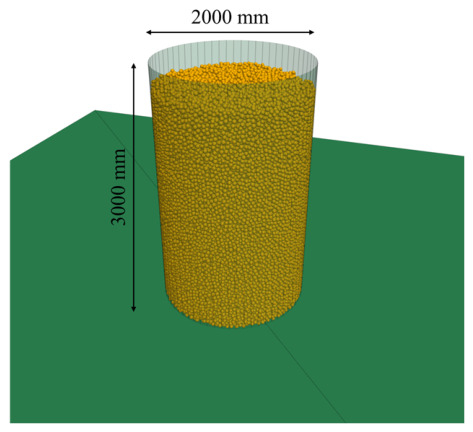
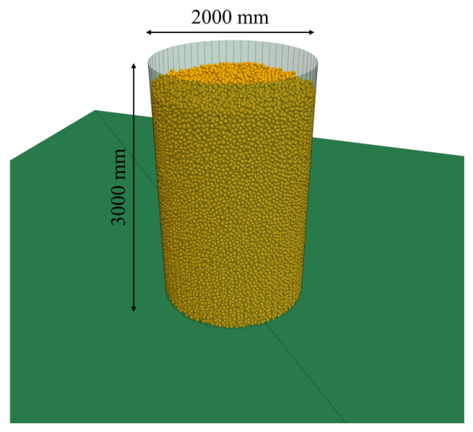
A foundation analysis model can be established by filling units within a limited analysis area. This study employed the falling method to randomly arrange and fill foundation elements, which utilizes the process of particles falling from high potential energy regions to low potential energy regions under the action of gravity to achieve model filling [9]. Its advantages include the ability to simulate the formation process of soil, establish close-to-actual construction conditions, and obtain a true internal stress distribution. A cylinder with a diameter of 2000 mm and a height of 3000 mm was generated, as depicted in Figure 5. Spherical particles of uniform diameter were used, resulting in an initial generation of 84,684 particles. The silt soil sample selected for the experiment consists of sand, silt, clay, and adhesive particles. Based on the representative fine particle size of , the linear particle size amplification factor is estimated at approximately 1000 [35,48].
Figure 5.
Assumed foundation data.
To ensure the simulation effect was close to the actual mixing effect on site, the drill rod and bit assembly (drill rod diameter 260 mm, blade diameter 1000 mm, and blade angle 30°) was modeled at full scale and imported into PFC 3D6.0, as depicted in Figure 3, with its attribute set to wall. The application of such mixing blades requires pre-set rotation, excavation, and contact parameters. Table 2 details the downmixing speed, uplifting speed, cement dosage, cement downmixing and uplifting ratio, and rotation speed set for the mixing blades. Given that the upper limit of the rotation speed of the mixing drilling rig in practical engineering is about 80 r/min, the simulation experiment was divided into two groups: the actual group and the hypothetical group. The practice group mainly focused on the achievable speed range for engineering construction, and the results obtained were used to correct and guide on-site applications, thereby providing quantitative reference for the optimal mixing speed under specific soil conditions. The hypothetical group explored the intrinsic correlation between rotational speed and stirring uniformity by expanding to a higher speed range (100–200 r/min). It should be noted that the hypothetical group is only accessible via DEM simulation and has not been realized in actual construction.
Table 2.
Simulation test plan and parameter settings.
Through this part of the research, the potential comprehensive value brought by increasing rotational speed could be evaluated and the critical yield value of uniformity with increasing rotational speed could be identified; that is, beyond this point, the contribution of rotational speed increase to improving uniformity was limited. In addition, because the effective cement content and mixing uniformity play an important role in the pile forming effect, further calculation of the corresponding effective cement content and analysis of the relationship between the three provided a scientific basis for optimizing the mixing speed for on-site construction, avoiding energy waste caused by blindly increasing equipment power. Moreover, it also helped to reveal the regularity of the mixing mechanism, which had reference value for the theoretical analysis and engineering application of relevant construction parameters. In addition, the simulation duration in this study is 300 s, corresponding to the early stage from spraying, shearing, and crushing to preliminary homogenization. This duration is considerably shorter than the initial setting time of cement. The model is intended to simulate the mixing process and evaluate uniformity during wet spray cement–soil mixing, rather than to predict the later-age strength or long-term service performance of cement soil.
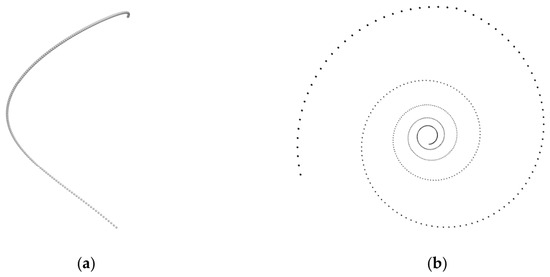
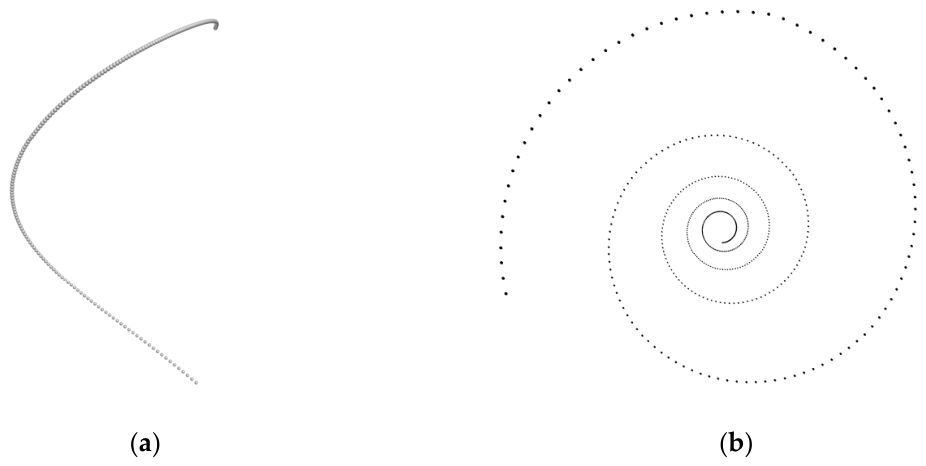
Of these, the cement content denotes the proportion of cement content to the mass of the mixed soil layer, which is represented by the number of balls generated. The process of cement particle spraying was implemented using the ball create command. To ensure the authenticity of the simulation, the generated position changed synchronously with the rotation of the drill rod, and the vertical displacement was the same. The synchronous simulation of the spraying and mixing of the drilling rig was achieved through a function loop, as displayed in Figure 6.
Figure 6.
Cement spraying process: (a) front view, (b) vertical view.
Taking the first set of experiments as an example, the complete process ranged from the drill bit contacting the soil layer to the bottom and then lifting from the bottom to the initial position, as displayed in Figure 7. After completion, the mixing model was saved, the parameters were changed, and the next set of simulation experiments commenced.
Figure 7.
Mixing process diagram.
5.2. Mixing Uniformity Analysis
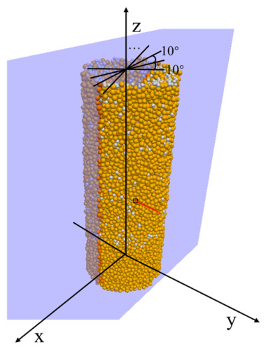
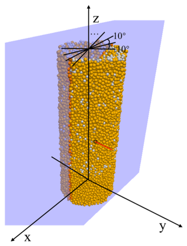
Cement–soil models were obtained after mixing at different rotational speeds, where cement particles were set to gray and soil particles were set to brownish red. Samples were taken according to the pile forming range (R = 0.5 m), and vertical cuts made according to the actual blade mixing range of 0 to −1.5 m. To further quantitatively analyze the mixing uniformity, a cross-section was taken every 10 degrees from 0° to 180° by rotating around the Z-axis, with a total of 18 positions taken, as depicted in Figure 8.
Figure 8.
Model cross-section.
The quantitative characterization of the particle mixing degree has a mature analytical system. To date, researchers investigating solid particle mixing have proposed various mixing degree evaluation methods to accurately describe the mixing state of the system, including the Mean Height Method [51], Nearest Neighbor Method [52], Neighbor Distance Method, Lacey Mixing Index Method [53], Mixing Entropy Method [54], Coordination Number Method, Particle Scale Index Method [55], and Siiri ä Method [56]. In previous work, a systematic comparison was made between the eight mixing degree calculation methods based on DEM simulation results. The results indicated that for the same mixed state, using different calculation methods may result in significantly different mixing index values. For example, in grid-based statistical methods such as Lacey’s method and mixed entropy method, there is a strong dependence on grid size; however, this may result in different mixed states being assigned the same degree of mixing, which is inconsistent with the actual physical situation. Therefore, in specific particle mixing studies, it has been necessary to choose a relatively suitable mixing degree evaluation method [57].
Among the numerous definitions of mixture degree, Danckwerts (1952) [58] proposed the mixture degree theory based on local concentration variance, which is one of the earliest and most representative methods. This method assumes that the mixed state can be measured by the ratio of the standard deviation of local component ratios to the theoretical maximum variance when not mixed at all and defines the normalized Danckwerts mixing index, which is used to measure the uniformity of particle mixing. The Danckwerts index was selected as the primary evaluation metric for the following reasons: First, the image analysis method employed in this study is based on the area fraction of the dominant particle color in each grid, denoted . The Danckwerts index is directly calculated from the standard deviation of , which aligns with the data processing approach adopted here. The value range of this indicator is from 0 to 1, and its basic principles are as follows:
- Local scale: First, divide the image into several equally sized grids according to the grid_size setting and then calculate the proportion of the main color (reddish brown) particles in each grid. The main color ratio of each grid can be represented as in Formula (5):where Amain,i and Aother,i are the pixel areas of primary and secondary color particles, respectively.
From this, the local proportional matrix {Pi} can be obtained, the spatial distribution of which reflects the local differences in the mixture.
- 2.
- Local proportional variance: Calculate the variance (var_local) of this local proportional , which measures the degree of change in the distribution of dominant color particles between different grids. The smaller the variance, the more uniform the particle distribution.
- 3.
- Standard Deviation (): Calculate the standard deviation of the local proportion of all effective grids, which reflects the fluctuation of particle distribution as in Formula (6):
- 4.
- Maximum standard deviation (): Calculate the maximum standard deviation of under the global proportion of the main color particles. The global proportion is the proportion of primary color particles to the total particles as in Formula (7):
- 5.
- Calculate MI_D using the following Formula (8):
To quantitatively evaluate the mixing uniformity of two-color particle systems, this study established a mixing degree calculation process suitable for discrete element simulation output images that was based on the mixing degree theory proposed by Danckwerts (1952) [58], combined with image processing and color clustering analysis methods. This index was chosen due to its clear definition, simple calculation, and lack of strong grid dependence. It is a method can automatically identify particle regions, separate particles of different colors, and calculate their spatial distribution characteristics, thereby generating the mixing uniformity index.
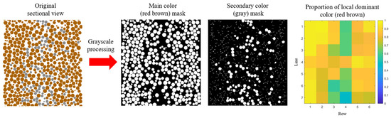
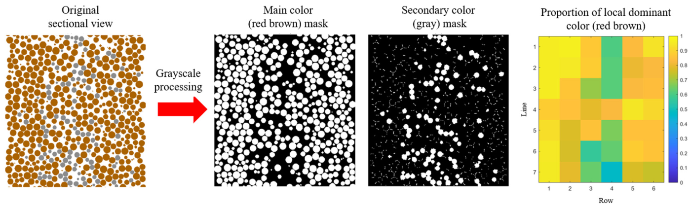
The method was then further implemented using MATLAB R2024a and the mixing uniformity of the dual color particle system was quantitatively evaluated in discrete element simulation using image processing techniques, as illustrated in Figure 9. Firstly, the original image was automatically cropped and the particle regions extracted, following which K-means clustering was used to identify reddish brown and gray particles in the CIELAB color space. Subsequently, the effective area was divided into grids, and the standard deviation of the proportion of main color particles within each grid was calculated.
Figure 9.
Image grid analysis.
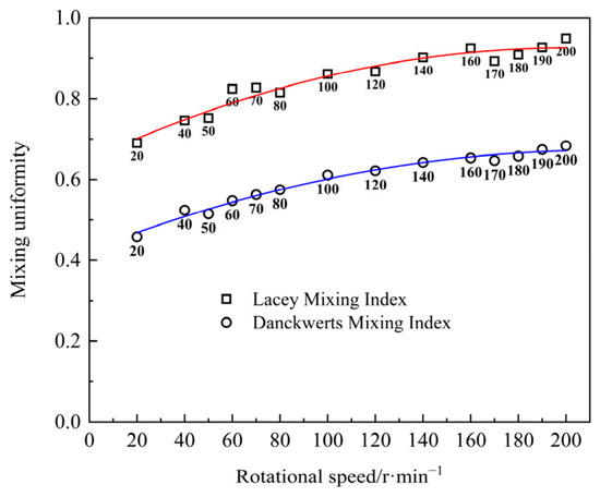
To ensure the consistency of the results, the Lacey index was supplemented as an auxiliary validation [54], which is defined as:
where N denotes the estimated equivalent number of particles in each grid.
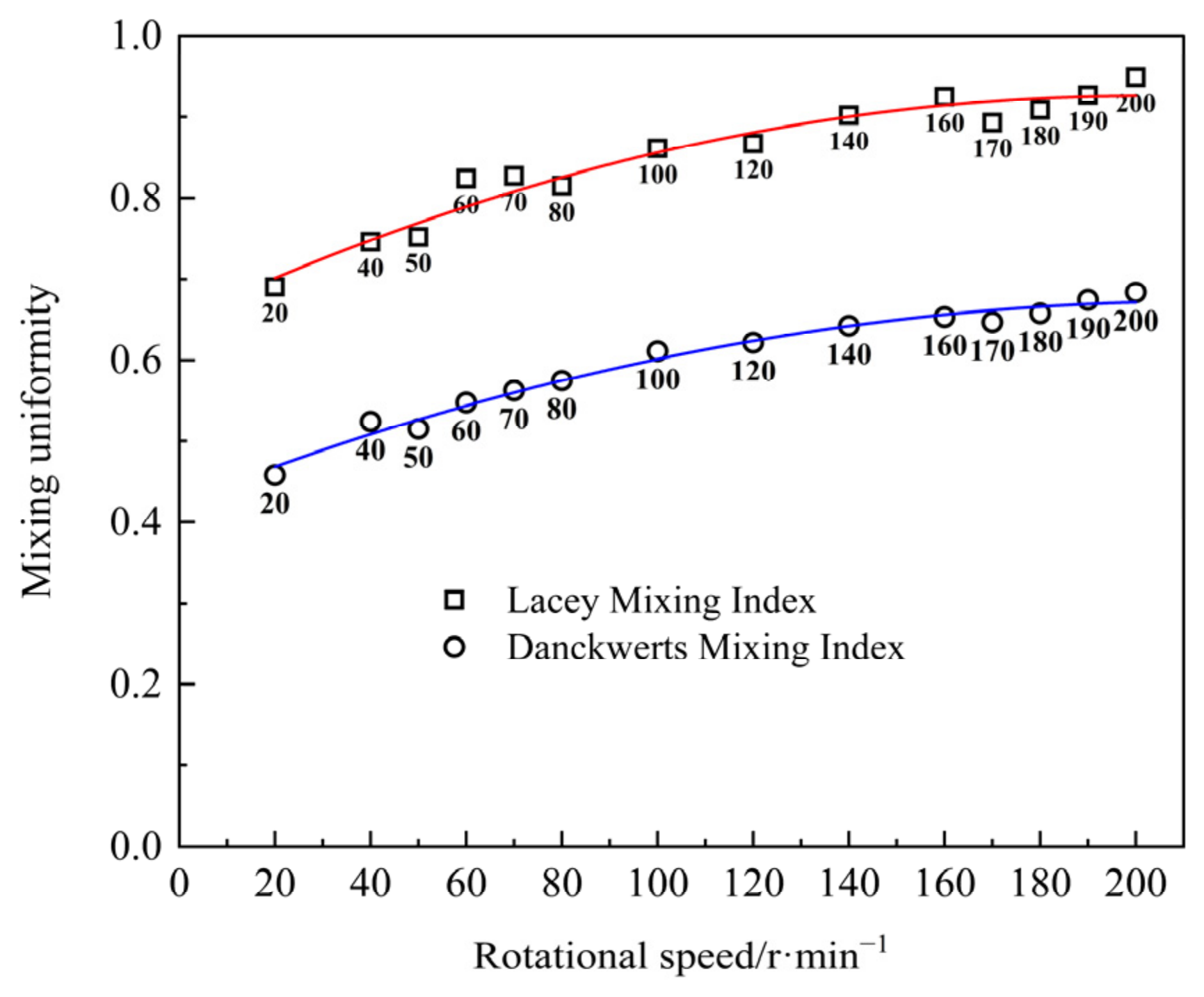
According to statistical principles, the grid edge length is usually assumed to be approximately 3 times the average particle diameter, with grid_size = 90 and N = 16. The calculated results are then plotted as a scatter plot of rotational speed and particle uniformity, as displayed in Figure 10.
Figure 10.
Curve of the relationship between stirring uniformity and rotational speed under two evaluation indices.
Comparison of the two curves reveals that their corresponding values are different but the trend of uniformity changes is consistent, indicating that the results are reliable and representative. According to Formula (11), the Lacey index is theoretically expected to be higher than the Danckwerts index in a moderately mixed system. Although their absolute values differ, both indices exhibit the same increasing trend with rotational speed, indicating that the mixing patterns captured by the two indicators are consistent. Thus, the results of the MI_D curve shall prevail in subsequent analysis.
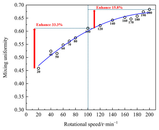
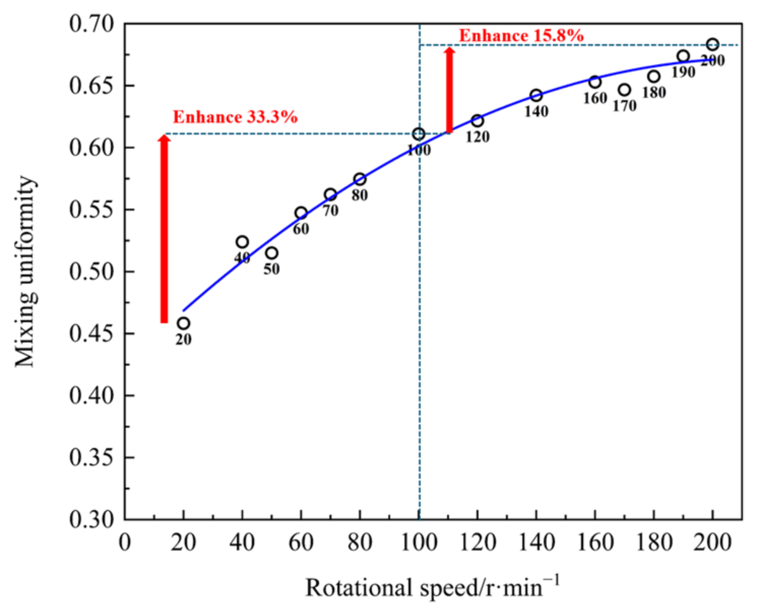
Based on the relationship between mixing uniformity and corresponding rotational speed, a standard curve (R2 = 0.98) was drawn, as shown in Figure 11. According to the development trend of the curve, uniformity increases in line with the increase in rotational speed, but the upward process can be divided into two stages: Stage 1—when the rotational speed is between 20 and 100 r/min, the uniformity and rotational speed maintain a linear growth relationship; and Stage 2—when the speed is 100–200 r/min, and the uniformity and speed maintain a decreasing growth relationship, with the slope of the curve gradually decreasing. Thus, when the speed exceeded 100 r/min, the effect of improving uniformity decreased significantly, with a difference of 17.5 percentage points in the magnitude of improvement before and after.
Figure 11.
Trend of uniformity with rotational speed.
5.3. Particle Mixing Behavior
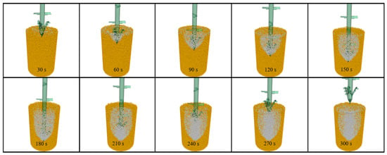
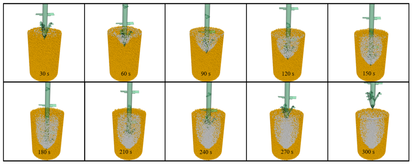
Given the strong relationship between the variation in uniformity and the rotational speed, it was necessary to analyze the behavior of soil particles during drilling and mixing to further explore its internal factors. At different rotational speeds, the three-dimensional motion behavior of the particles was approximate. Taking the hypothetical group with a rotational speed of 120 r/min as an example, Figure 12 depicts the simulation results obtained when mixing the hypothetical foundation with a mixing drilling tool using the wet water spraying soil mixing method.
Figure 12.
Mixing process effect diagram.
Through three-dimensional visualization, the particle behavior during wet spraying and mixing can be clearly observed: from 0 to 60 s, the drill bit initially intruded into the soil and destroyed the original structure of the soil particles, causing the undisturbed soil particles to shift in all directions, forming a V-shaped excavation cavity. At this point, the cement particles ejected from the nozzle were subjected to the shear and suction effects of the drilling tool rotation, forming an initial mixing core near the drill tip. In addition, cement particles underwent local filling and preliminary radial diffusion in the shear failure zone [59]. At 60–180 s, as the drilling tool continued to sink and spray, cement particles expanded outward in a spiral fan shape with the blades. Under the shearing and spiral pushing of the blades, the mixing zone continued to widen, initially forming a mixed body. At 180–300 s, when the drilling tool reached the bottom and switched to an upward state, the existing mixing zone was subjected to secondary disturbance, triggering a new round of radial and axial diffusion. The cement slurry moved up with the nozzle and filled the central cavity area layer by layer along the spiral channel. Another round of rotational shear further strengthened the soil particles in the middle and upper areas, ultimately forming a cement–soil mixture [59].
In summary, the mixing mechanism of the wet spray mixing method for silty soil lies in the joint drive of high blade shear and spiral conveying. As cement particles diffuse towards the periphery, they are affected by centrifugal force and the wall blockage of undisturbed soil surrounding them. The particles are prone to form circumferential bands and local backflow at the edges, filling the peripheral poor slurry area [60,61,62]. This mechanism further confirms that rotational speed plays an important role in the stirring process, as it affects the shear strain rate around the drill bit and blades. According to the rheological laws of non-Newtonian fluids, an increase in shear strain rate significantly reduces the viscosity of the local mixture [63,64]. This significantly reduces the resistance to relative motion between particles, making it easier for cement particles to penetrate the interior of undisturbed soil clusters, thereby improving micro uniformity. However, based on the previous analysis, although increasing the rotational speed can improve the uniformity of stirring, this gain is nonlinear. When the rotational speed exceeds a certain critical threshold, excessive centrifugal force may cause excessive outward diffusion of cement particles; therefore, a rotational speed range may exist that achieves the optimal balance between mixing and diffusion.
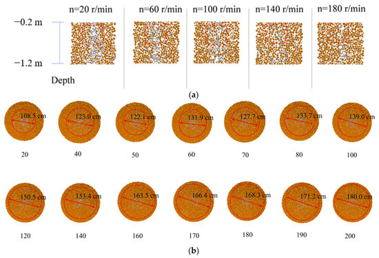
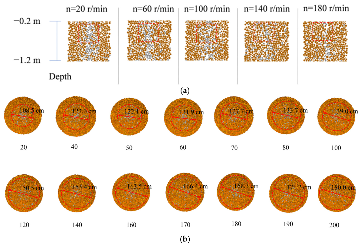
5.4. Rotational Speed Balance Range
According to previous calculations, the rotational speed increased by nearly 10 times from 20 r/min to 200 r/min, but the improvement in uniformity did not achieve the effect of quantitative change and qualitative change. From the above particle behavior, it is apparent that some cement particles were affected by high rotational speed and continued to diffuse outside the pile or on the surface. The vertical profile of the model was then cut within a radius of 1 m, with a depth ranging from −0.2 to −1.2 m, and a horizontal profile at a depth of −1.2 m, as displayed in Figure 13. As depicted in Figure 13a, most of the aggregated cement particles were continuously cut and gradually diffused as the rotational speed increases, and a portion was squeezed out of the pile diameter range. As the concentration of cement particles gradually decreased, more cement particles concentrated in the blind spots of blade mixing, further increasing the difficulty of improving uniformity. As shown in Figure 13b, with the increase in rotational speed, the range of outward diffusion of cement particles increased, which is akin to the soil squeezing effect in actual engineering. At low rotational speeds, the cement particles at the center were more concentrated, and the distribution of cement particles outside the designed pile diameter was reduced. At high rotational speed, the cement particles at the center were uniformly dispersed, while the number of cement particles on the outer side slowly increased.
Figure 13.
Distribution of cement particles at different rotational speeds: (a) horizontal section, (b) vertical section.
The effective content of cement in the pile and its uniform distribution in the soil significantly impact the solidification strength of cement–soil piles. It primarily determines the amount of hydration products generated, thereby controlling the upper limit of strength [65,66]. The uniformity of mixing affects the continuity of the bond between cement and soil particles, determining the effective degree of strength realization [67]. Due to the combined effects of construction technology, moisture content, pore structure, and water–cement ratio, the sensitivity of cement dosage and mixing uniformity to the solidification strength of cement soil is not fixed but fluctuates within a certain range in line with changes in actual working conditions. Under conditions of uniform mixing and good construction control, the main effect of cement dosage can explain approximately 60% of the change in strength [65,66]. In environments with high porosity, high water content, or significant construction disturbance, the contribution or negative impact of mixing uniformity factors can be amplified to a level equivalent to the cement content [67,68,69,70]. For example, Ge et al. [71] conducted model experiments based on a powdery clay foundation and found that increasing the cement content from 8% to 18% after seven days of curing increased the compressive strength of cement–soil samples by 220%, the strength by 300%, and the total number of blade rotations from 386 r/min to 1414 r/min. Therefore, in both design and construction, attention should be paid to the control of mixing uniformity and effective cement content to ensure the stability and reliability of cement–soil pile strength. The effective cement content generally needs to be close to the cement dosage, reaching more than 80% of the designed cement dosage.
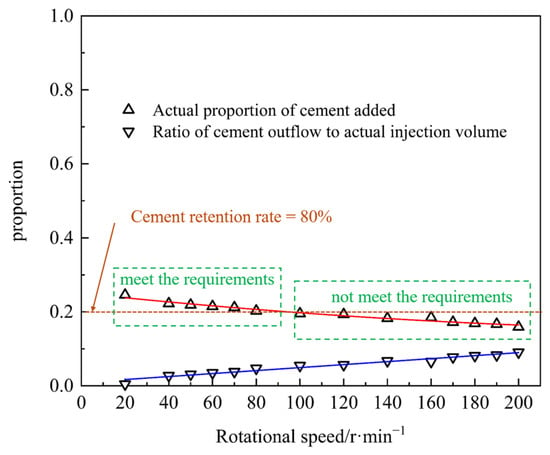
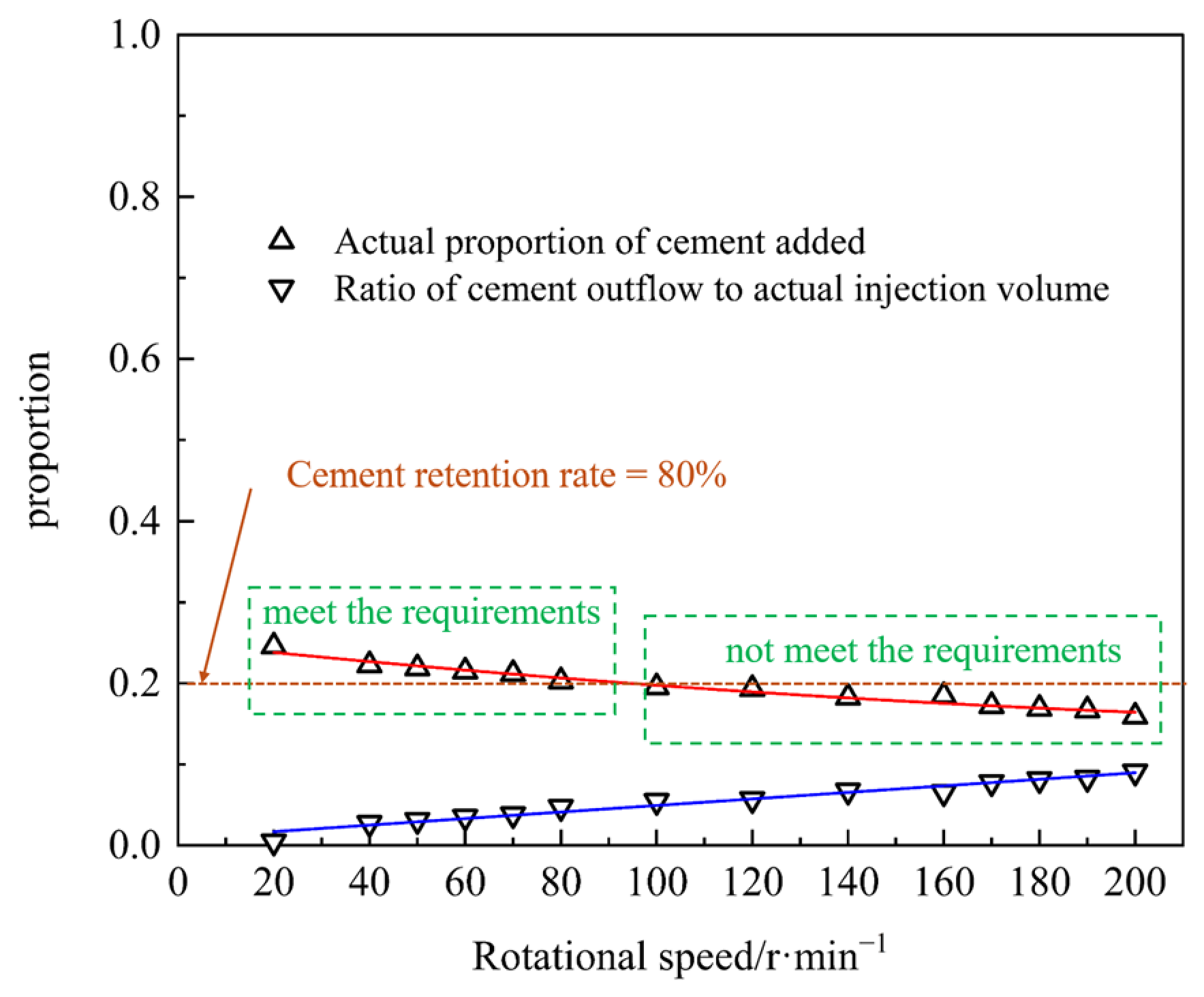
To that end, further quantitative indicators were used to calculate and analyze the effective cement content inside the pile, as displayed in Figure 14.
Figure 14.
Trend of effective cement content and discharge with rotational speed.
As indicated in Figure 14, with an increase in rotation speed, the proportion of cement pouring out continuously increased, while the effective content of cement in the pile slowly decreased. When the rotational speed exceeded 100 r/min, the cement retention rate inside the pile began to drop below 80%, which does not meet the standard. At rotational speeds ranging from 20 to 80 r/min, the proportion of cement particles within the pile forming range was relatively high. Based on the conclusions reached in previous chapters, the higher the rotational speed, the more likely it is that the uniformity cannot achieve sustained high growth, indicating the existence of a rotational speed balance range that ensures high mixing uniformity and meets the effective cement content standard. However, the above results still need to be verified through on-site experiments.
5.5. Engineering Feasibility Analysis
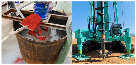
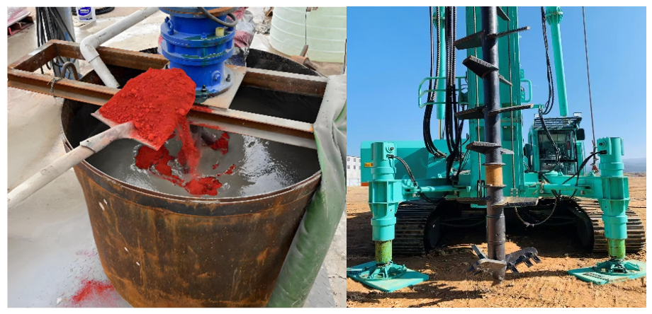
Based on the speed range obtained in Section 5.4, the rotational speeds were set to 40 r/min, 60 r/min, and 80 r/min for on-site practice. The test site, located in the Nansha area of Guangdong Province, comprises a 0–2 m mixed soil layer overlying a 2–18 m silt layer. The on-site tests focused on the silt layer, which had a natural moisture content of 45%, a density of 1.66 g/cm3, and a porosity of 50%. During the pulping process, iron red slurry was added for staining, as shown in Figure 15, to facilitate subsequent sampling and observation. The assembly used in the on-site test was identical in shape and dimensions to that employed in the simulation. After 3 days of on-site construction, the geological drilling rig was used for core sampling. The cement–soil test block was cured in a standard curing room at a temperature of 20 ± 2 °C and a relative humidity above 95% for 28 days.
Figure 15.
On-site pulping and sampling diagram.
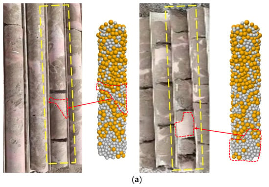
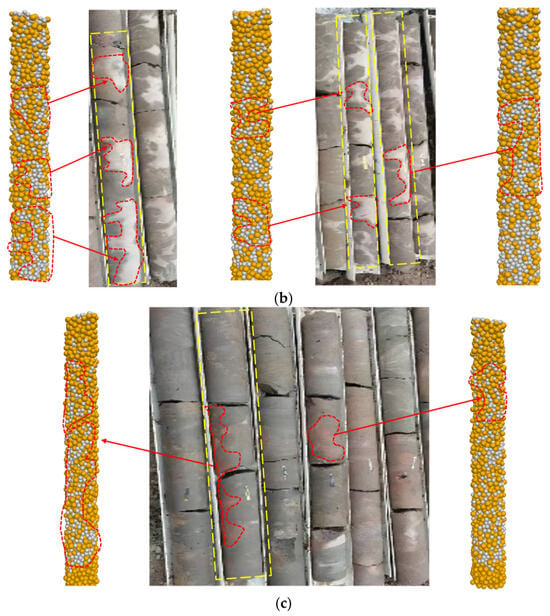
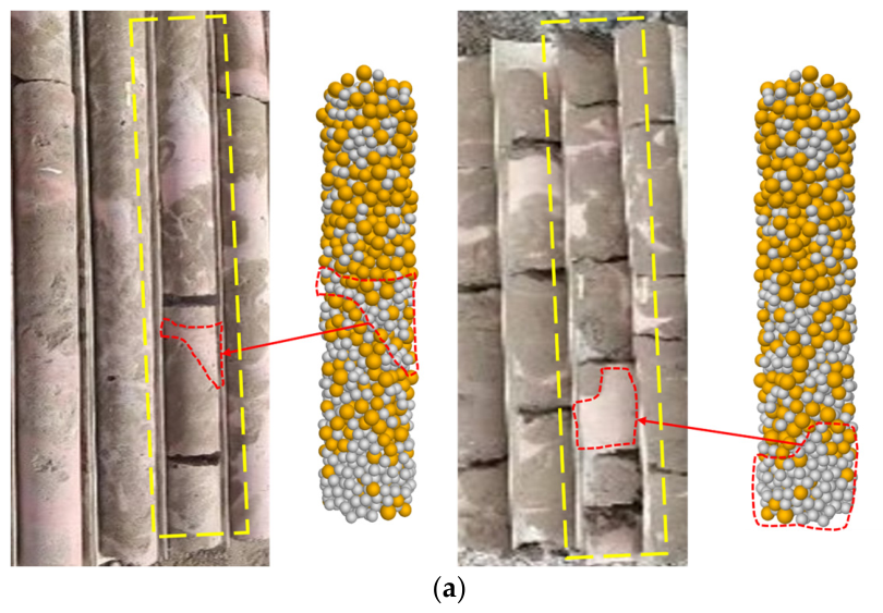
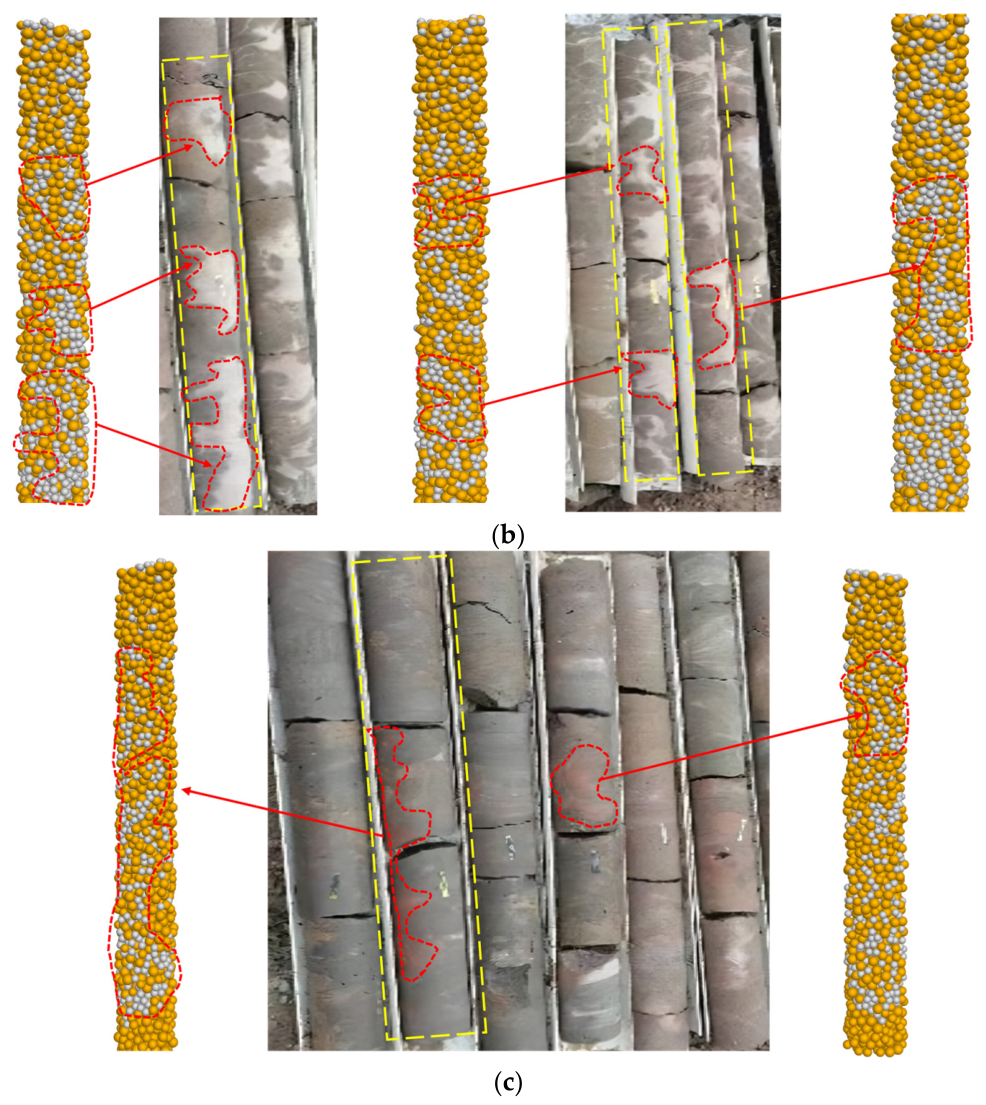
Comparing the sampling results with the simulation results, as depicted in Figure 16, it can be observed that in terms of the distribution of cement particles, most of the surface areas of the simulated cement–soil mixing pile correspond to the actual sampling results, forming a certain irregular shape. Moreover, from the sampling effect, the cement–soil core sample formed at 40 r/min created cement particle aggregation in some areas, indicating incomplete mixing. Based on the surface distribution, the cement soil formed at 60 r/min reflects a certain improvement in mixing uniformity compared with 40 r/min. The cement soil formed at 80 r/min also has good uniformity but, compared with the sampling effect at 60 r/min, there is no significant improvement.
Figure 16.
Comparison between simulation results and on-site sampling: (a) sampling effect of cement–soil pile at 40 r/min, (b) sampling effect of cement–soil pile at 60 r/min, (c) sampling effect of cement.
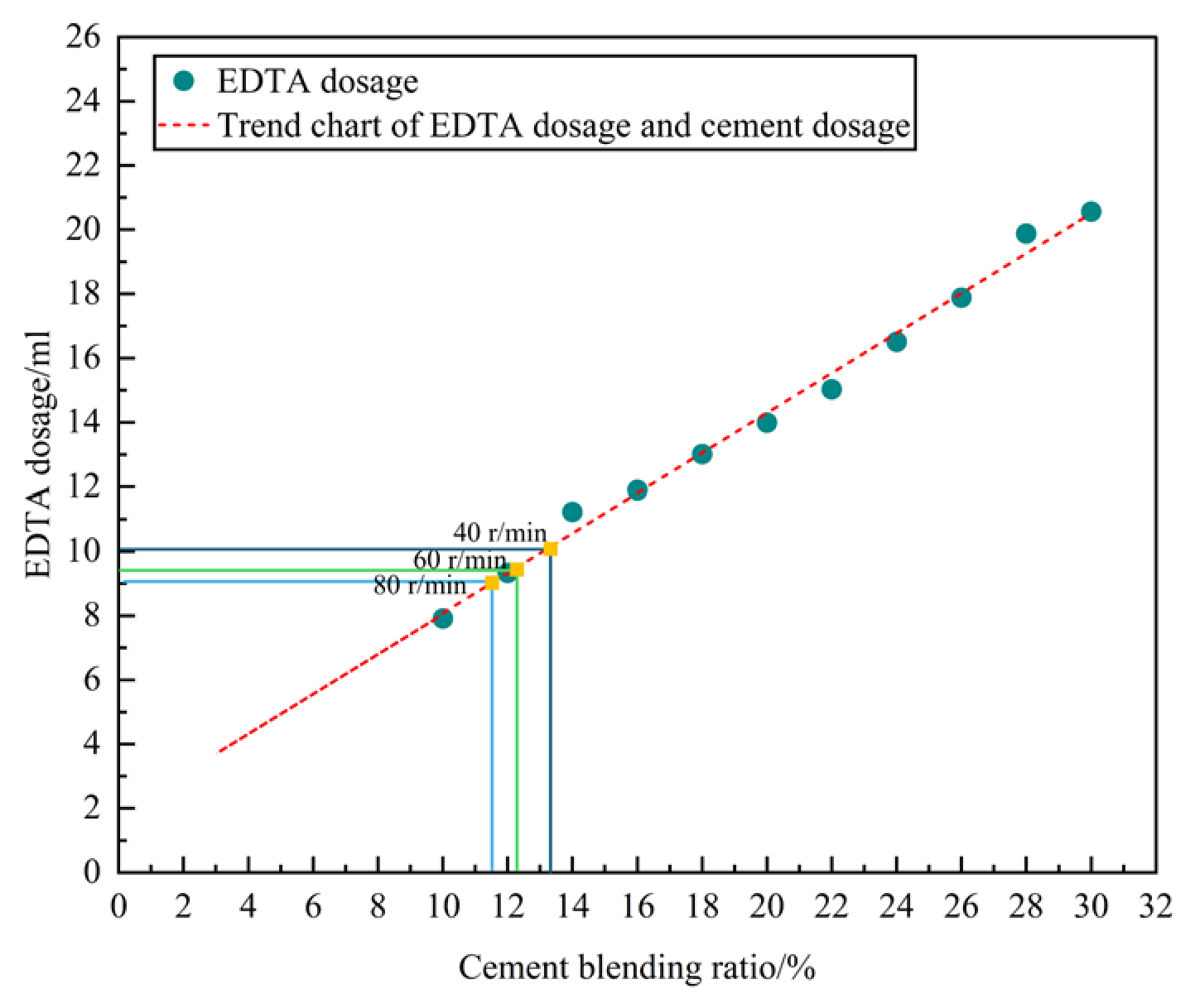
According to the simulation results in Section 5.4, the effective cement content will slowly decrease with increasing rotational speed. To further verify the reliability of this result, the EDTA titration method was used to measure the effective cement content of the cement mixing pile [72]. In situ soil samples were taken and mixed with cement slurry of different dosages. The water–cement ratio of the cement slurry was the same as that of the on-site construction (both 0.8) and the cement dosage was 10% to 30%, with an interval of 2%. In situ soil with different cement dosages was then mixed and sealed for the same number of days as the previous sample. Following this, the compacted part was crushed and the supernatant was fully mixed to prepare a standard slurry. To achieve this, 300 g of mud was mixed with 600 mL of 10% NH4Cl solution and stirred for 3 min. The mixture was then allowed to stand for 20 min. Next, 10 mL of the supernatant was placed in a triangular flask. Following this, 0.2 g of calcium red indicator and 50 mL of 1.8% NaOH (containing triethanolamine) solution were added to the flask, which was shaken well. The EDTA disodium standard solution was then placed into an acid burette for titration. The amount of EDTA disodium standard solution used was then recorded and a standard curve (R2 = 0.992) drawn based on the relationship between the consumption of EDTA disodium standard solution and the corresponding mud, which is expressed by Formula (12):
where Y denotes the EDTA dosage, and x denotes the cement blending ratio.
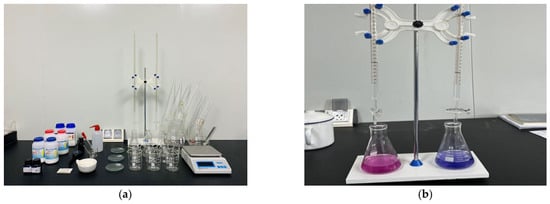
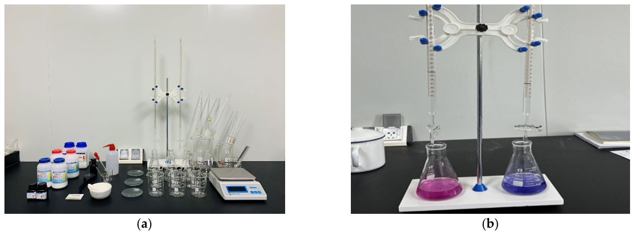
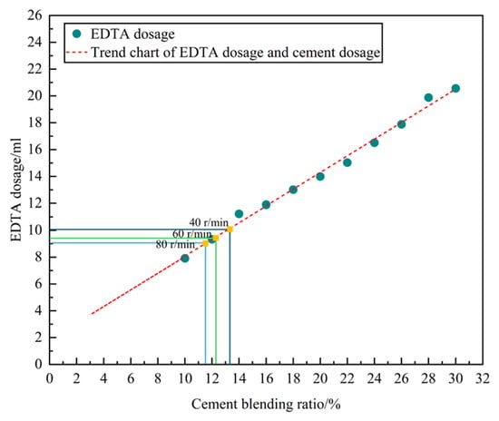
After obtaining the standard curve, the effective cement content in the cement–soil mixing pile was accurately determined through an indoor titration test (Figure 17), as displayed in Figure 18.
Figure 17.
EDTA indoor titration test: (a) experimental equipment, (b) titration of effective content of recycled cement.
Figure 18.
Titration results of effective cement content (35 d).
Subsequently, EDTA titration tests were conducted on cement–soil mixing piles (with a cement content of 15%) obtained at different rotational speeds on the construction site. The corresponding consumption of the EDTA disodium standard solution was compared with the standard curve to determine the effective content of cement. The results of the titration test are presented in Figure 18. The corresponding results of the three sets of rotational speeds are depicted in Figure 18. From the data, the effective cement content in the pile was 13.11% at a rotational speed of 40 r/min, 12.26% at a rotational speed of 60 r/min, and 11.53% at a rotational speed of 80 r/min. The corresponding cement retention rates were 87.40%, 81.72%, and 76.84%, respectively. According to the trend of change, as the rotational speed increased, the cement retention rate inside the pile slowly decreased, which is similar to the trend reflected in the simulation results.
Overall, when the mixing speed was between 40 and 60 r/min, the cement–soil pile formation effect improved, the integrity of on-site sampling was better, the surface cement distribution was more uniform, and the measured cement retention rate was at a reasonable level; that is, greater than 80%. This further verifies the effectiveness of the simulation and the feasibility of subsequent on-site applications. In addition, compared with a speed of 80 r/min, it can also reduce energy consumption and construction costs in terms of motor power output. Engineering practice shows that blindly increasing the rotational speed can lead to higher energy consumption per unit volume, accelerated wear of drill rods and transmission systems, more frequent maintenance of nozzles and seals, and greater volumes of slurry return and waste treatment. As indicated by Formula (13), when the pile diameter, cutting speed, and torque lie within typical engineering ranges, increasing the rotational speed from 60–80 r/min to 100–120 r/min will significantly raise the equipment’s operating power and thus its energy consumption.
where P is power, n is rotational speed, and Tq is torque.
This study introduced the DEM to reproduce and analyze the process of foundation improvement, compensating for the shortcomings of traditional methods that are difficult to visualize and quantitatively detect. By applying the three-dimensional DEM in the early design stage of foundation improvement technology, the improvement effect can be predicted in advance, thereby reducing the number of experiments and rework, greatly improving research and development efficiency and cost control capabilities. Moreover, flexible control of multi-dimensional working conditions can be achieved in virtual environments. By leveraging the modeling and simulation advantages of the PFC 3D6.0 platform, it is possible to track the soil response and mix energy transfer process at the particle scale, deepen understanding of the mechanism of foundation improvement, and improve the reliability and adaptability of the scheme. The research results indicate that the PFC 3D6.0-based computer simulation method has good feasibility and potential for promotion in foundation improvement analysis. It can not only predict improvement effects in the early stage of technological development, reduce testing, and rework costs, but, in subsequent research, can also provide a scientific basis for blade structure optimization and construction parameter selection through detailed simulation of the mixing blade effect in the wet water spraying soil mixing method, thereby improving the visualization level and engineering adaptability of the improvement process [73]. More importantly, to quantitatively evaluate its potential effectiveness, this method can be extended to technical means or extreme working conditions that cannot be directly achieved under current engineering conditions. This not only provides an optimization direction and theoretical support for on-site construction but also helps to avoid insufficient economic benefits caused by a lack of experience or blind design, which has important theoretical value and practical significance.
It should be noted that the rotational speed balance range provided in Section 5.4 is for reference only. This interval value is closely related to the actual soil conditions, drilling rig design, and actual construction parameters, but its existence also indicates that there is indeed a better mixing speed under certain conditions. In practical engineering, this can be initially determined through numerical simulation or on-site testing, providing an auxiliary basis for construction. This conclusion also highlights the direction for future work in this area. For instance, further research can explore the impact of more process parameters on pile quality and efficiency and analyze the interaction laws between multiple parameters. In addition, by collecting and accumulating parameter data under different soil conditions, corresponding databases can be established to achieve systematic correlation between various soil layers and their corresponding speed balance ranges, providing more scientific guidance for engineering design and construction optimization.
6. Conclusions
This study aimed to explore the effectiveness and value of increasing rotational speed in improving the mixing uniformity of silty soil and cement. The three-dimensional DEM was applied to conduct three-dimensional modeling, parameter calibration, and experimental reproduction of the entire process of mixing drilling tools, construction sites, and the wet spraying cement–soil mixing method. Combined with image recognition, the Danckwerts mixing index was introduced to output quantitative results on the mixing uniformity of water and soil at different rotational speeds. Further research is required to determine the influence of rotational speed on stirring uniformity, develop a systematic evaluation and optimization method for rotational speed parameters, and verify this method through field experiments and titration experiments. The specific results are as follows:
- (1)
- A three-dimensional DEM was established for the entire process of wet water spraying soil mixing. Through numerical modeling of real drill rods and mixing blades, as well as accurate parameter calibration and process control, the flow and mixing behavior of silty soil and cement slurry during the construction process were reproduced. This model provides a feasible computational basis for revealing the mixing mechanism and optimizing construction parameters from a microscopic perspective.
- (2)
- The law of the variation in mixing uniformity with rotational speed was explored in this research. By combining Danckwerts blending theory with the CIELAB color space clustering algorithm, automatic recognition and spatial distribution analysis of the dual color particle system were achieved, forming a quantitative process for evaluating mixing uniformity. The simulation results revealed that mixing uniformity increased in line with the increase in rotational speed, but the rate of uniformity improvement is significantly small with the rotational speed improvement.
- (3)
- The particle movement mechanism during the entire process of wet water spraying soil mixing was revealed. The mixing of two types of particles is driven by both blade high shear and spiral conveying. The rotational speed reduces the viscosity of undisturbed soil particles by increasing the shear strain rate, promoting the infiltration of cement particles. In conjunction with this, cement particles diffuse under centrifugal force and wall blockage, forming a circumferential band and local reflux, filling the poor slurry area, and improving micro uniformity.
- (4)
- A calculation method for determining the speed balance interval was established using mixing uniformity and effective cement content within the pile forming range as reference criteria. By calculating the rotational speed balance range, energy consumption and material loss can be reduced while ensuring the quality of the pile and mixing uniformity, which has significant engineering guidance value.
- (5)
- The feasibility of using agitation simulation to guide engineering practice was verified through EDTA experiments. Based on the research results of model agitation tests on silty soil foundations, this approach is mainly applicable to silty soil layers and provides a quantitative basis for rotational speed optimization.
Author Contributions
Methodology, X.J.; software, B.H.; validation, W.S.; formal analysis, W.S.; investigation, B.L., X.J. and X.Y.; resources, B.L.; data curation, B.H.; writing—original draft preparation, B.H.; writing—review and editing, W.S.; visualization, B.H.; supervision, W.S., X.J. and X.Q. All authors have read and agreed to the published version of the manuscript.
Funding
This research was funded by the National Key Research and Development Program of China (2022YFE0200400).
Data Availability Statement
The data presented in this study are available on request from the corresponding author. The data are not publicly available due to privacy and ethical restrictions.
Conflicts of Interest
Authors Weijie Song and Xiaocheng Qu were affiliated with the company Beijing Anke Xingye Technology Co., Ltd. Authors Weijie Song, Boran Huang and Bo Liu were affiliated with the company Beijing Zhongyan Dadi Technology Co., Ltd. The remaining authors declare that the research was conducted in the absence of any commercial or financial relationships that could be construed as a potential conflict of interest.
Abbreviations
The following abbreviations are used in this manuscript:
| DEM | Discrete element method |
| Arrlinear | Adhesive rolling resistance linear |
References
- Huang, F.; Chen, Z.; Deng, H.; Zhu, W. Lateral deformation mechanisms of piles in coastal regions under seawall surcharge loading and mitigation using deep cement mixing (DCM) piles. Buildings 2025, 15, 1936. [Google Scholar] [CrossRef] [Scilit]
- Yin, K.S.; Xiao, T.; Luo, H.Y.; Zou, H.F.; Zhang, L.M. Probabilistic modeling of offshore deep cement mixing improved ground. Comput. Geotech. 2023, 156, 105266. [Google Scholar] [CrossRef] [Scilit]
- Lu, C.R.; Zhang, X.H.; Shi, B.B.; Jiang, J.Q.; Lin, Z.R. Deformation in settlement and grouting remediation of thickened larger-diameter metro shield tunnel in soft soil: A case study. Case Stud. Constr. Mater. 2024, 20, e02736. [Google Scholar] [CrossRef] [Scilit]
- Xiong, J.G.; Gong, Y.Q.; Liu, X.H.; Li, Y.; Chen, L.J.; Liao, C.; Zhang, C.C. A PSO-XGBoost Model for Predicting the Compressive Strength of Cement–Soil Mixing Pile Considering Field Environment Simulation. Buildings 2025, 15, 2740. [Google Scholar] [CrossRef] [Scilit]
- Wu, K.; Zhang, P.; Yuan, J.J.; Qian, X.Q.; Qi, R.N. IoT Monitoring and Evaluating System for the Construction Quality of Foundation Pile. Buildings 2025, 15, 2660. [Google Scholar] [CrossRef] [Scilit]
- Hong, J.Q.; Yan, Z.; Bao, H.; Fang, H.; Zhu, W.H.; Zhang, S.F. Analytical solution of the internal interface stress in composite piles under confining pressure. Case Stud. Constr. Mater. 2026, 24, e06029. [Google Scholar] [CrossRef] [Scilit]
- Deng, T.T.; Deng, Y.F.; Fisonga, M.; Liu, S.Y.; Wu, Y.S.; Dai, H. Revisiting mixing uniformity effect on strength of cement-based stabilized soft clay. J. Rock Mech. Geotech. Eng. 2024, 16, 5221–5230. [Google Scholar] [CrossRef] [Scilit]
- Zhu, Z.D.; Liu, S.Y.; Xi, P.S.; Zhou, L.H. Analysis of effect of T-shaped bidirectional soil–cement deep mixing columns reinforcing soil foundation. Rock Soil Mech. 2009, 30, 2063–2067. [Google Scholar] [CrossRef]
- Xu, C.; Dong, T.L.; Ye, G.B. Application of cement deep mixing method in Lianyungang marine soft soil foundation. Rock Soil Mech. 2006, 27, 495–498. [Google Scholar] [CrossRef]
- Liu, H.; Yang, S.F.; Bian, X.Y.; Zhou, H. Study on the bearing characteristics of composite foundations with permeable concrete piles. Appl. Sci. 2025, 15, 4835. [Google Scholar] [CrossRef] [Scilit]
- Zhou, A.Z.; Wang, H.N.; Huang, R.D.; Wang, W.; Liu, G.; Xu, N.; Yin, J. Enhancement-type graphene treated cement-soil for building foundation improvement: Experimental and microscopic investigations. J. Build. Eng. 2025, 114, 114251. [Google Scholar] [CrossRef] [Scilit]
- Liu, D.W.; Huang, L.L.; Li, J.L.; Shen, Q.S. Formulation and performance of nano-composite clay-cement based grouting materials in water-bearing sandy soil. Case Stud. Constr. Mater. 2024, 21, e03891. [Google Scholar] [CrossRef] [Scilit]
- Zhang, R.H.; Zhou, J.J.; Gong, X.N.; Ming, W.; Wang, T. Experimental and DEM simulation on engineering properties of soft soil stabilized by industrial solid waste—Cement synergy. Case Stud. Constr. Mater. 2025, 22, e04852. [Google Scholar] [CrossRef] [Scilit]
- Porbaha, A.; Tanaka, H.; Kobayashi, M. State of the art in deep mixing technology: Part II. Applications. Proc. Inst. Civ. Eng. Ground Improv. 1998, 2, 125–139. [Google Scholar] [CrossRef] [Scilit]
- Li, Z.; Kasama, K.; Hu, L.H.; Yu, J.Y.; He, Y.; Yahiro, Y.C. The strength evaluation of cement-mixed soil considering mixing quality using image analysis and Bayesian approach. Comput. Geotech. 2025, 183, 107225. [Google Scholar] [CrossRef] [Scilit]
- Inazumi, S.; Jotisankasa, A.; Nakao, K.; Chaiprakaikeow, S. Performance of mechanical agitation type of ground-improvement by CAE system using 3-D DEM. Results Eng. 2020, 6, 100108. [Google Scholar] [CrossRef] [Scilit]
- Yang, H.P.; Ma, G.G.; Zhao, W. DEM-Based Simulation Study on the Operational Performance of a Single Horizontal Shaft Forced-Action Mixer. Buildings 2025, 15, 2627. [Google Scholar] [CrossRef] [Scilit]
- Lin, R.; Ren, L.; Zhao, J.Z.; Tan, X.C.; Rasouli, V.; Wang, X.; Shen, C. Stress and pressure dependent permeability of shale rock: Discrete element method (DEM) simulation on digital core. J. Pet. Sci. Eng. 2022, 208, 109797. [Google Scholar] [CrossRef] [Scilit]
- Nitka, M. Static and dynamic concrete calculations: Breakable aggregates in DEM model. J. Build. Eng. 2024, 89, 109006. [Google Scholar] [CrossRef] [Scilit]
- Feng, Y.T.; Owen, D.R.J. Discrete element modelling of large-scale particle systems—I: Exact scaling laws. Comput. Part. Mech. 2014, 1, 159–168. [Google Scholar] [CrossRef] [Scilit]
- Milkevych, V.; Munkholm, L.J.; Chen, Y.; Nyord, T. Modelling approach for soil displacement in tillage using discrete element method. Soil Tillage Res. 2018, 183, 60–71. [Google Scholar] [CrossRef] [Scilit]
- Wang, Y.; Zhang, D.; Yang, L.; Cui, T.; Jing, H.; Zhong, X. Modeling the interaction of soil and a vibrating subsoiler using the discrete element method. Comput. Electron. Agric. 2020, 174, 105518. [Google Scholar] [CrossRef] [Scilit]
- Huang, H.; Wang, P.T.; Huang, B.R.; Jing, G.Y.; Cai, M.F. Fracturing characteristics of unconfined rock plate subjected to point-plate loading. Eng. Fract. Mech. 2025, 319, 111047. [Google Scholar] [CrossRef] [Scilit]
- Ucgul, M.; Saunders, C. Simulation of tillage forces and furrow profile during soil–mouldboard plough interaction using discrete element modelling. Biosyst. Eng. 2020, 190, 58–70. [Google Scholar] [CrossRef] [Scilit]
- Wilson, R.; Dini, D.; Van Wachem, B. The influence of surface roughness and adhesion on particle rolling. Powder Technol. 2017, 312, 321–333. [Google Scholar] [CrossRef] [Scilit]
- Wu, A.Z.; Zhang, Z.N.; Shi, X.; Liu, C.L. Modeling the role of interfacial adhesion in the rolling resistance of a hyperelastic wheel. Tribol. Int. 2023, 185, 108494. [Google Scholar] [CrossRef] [Scilit]
- Boschi, K.; di Prisco, C.G.; Ciantia, M.O. Micromechanical investigation of grouting in soils. Int. J. Solids Struct. 2020, 187, 121–132. [Google Scholar] [CrossRef] [Scilit]
- Nazari, R.; Papangelo, A.; Ciavarella, M. Friction in rolling a cylinder on or under a viscoelastic substrate with adhesion. Tribol. Lett. 2024, 72, 50. [Google Scholar] [CrossRef] [Scilit]
- Wu, Z.Y.; Wang, X.S.; Liu, D.W.; Xie, F.P.; Ashwehmbom, A.L.G.; Tang, Z.Z.; Tang, Q.J. Calibration of discrete element parameters and experimental verification for modelling subsurface soils. Biosyst. Eng. 2021, 212, 215–227. [Google Scholar] [CrossRef] [Scilit]
- Zhou, L.; Lan, Y.B.; Yu, J.Q.; Wang, Y.; Yan, D.X.; Sun, K.; Chen, Y.L. Validation and calibration of soil parameters based on EEPA contact model. Comput. Part. Mech. 2023, 10, 1295–1307. [Google Scholar] [CrossRef] [Scilit]
- Cundall, P.A.; Strack, O.D.L. A discrete numerical model for granular assembles. Geotechnique 1979, 29, 47–65. [Google Scholar] [CrossRef] [Scilit]
- Magnier, S.A.; Donzé, F.V. Numerical simulations of impacts using a discrete element method. Mech. Cohesive-Frict. Mater. 1998, 3, 257–276. [Google Scholar] [CrossRef]
- Rowe, P.W. The stress-dilatancy relation for static equilibrium of an assembly of particles in contact. Proc. Math. Phys. Eng. Sci. 1962, 269, 500–527. [Google Scholar] [CrossRef] [Scilit]
- Gilabert, F.A.; Roux, J.N.; Castellanos, A. Computer simulation of model cohesive powders: Influence of assembling procedure and contact laws on low consolidation states. Phys. Rev. E 2007, 75, 011303. [Google Scholar] [CrossRef] [Scilit] [PubMed]
- Nakao, K.; Inazumi, S.; Takaue, T.; Tanaka, S.; Shinoi, T. Evaluation of Discharging Surplus Soils for Relative Stirred Deep Mixing Methods by MPS-CAE Analysis. Sustainability 2021, 14, 58. [Google Scholar] [CrossRef] [Scilit]
- Li, H.J.; Liu, S.Y.; Tong, L.Y. Field investigation of the performance of composite foundations reinforced by DCM-bored piles under lateral loads. Constr. Build. Mater. 2018, 170, 690–697. [Google Scholar] [CrossRef] [Scilit]
- Zyka, K.; Mohajerani, A. Composite piles: A review. Constr. Build. Mater. 2016, 107, 394–410. [Google Scholar] [CrossRef] [Scilit]
- Yang, Z.J.; Chen, K.X.; Fu, X.D.; Zou, Z.Y. Effects of cement-enhanced soil on the ultimate lateral resistance of composite pile in clayey soil. J. Rock Mech. Geotech. Eng. 2024, 16, 183–191. [Google Scholar] [CrossRef] [Scilit]
- Li, W.; Kwok, C.Y. Engineering behaviour of in situ cored deep cement mixed marine deposits subjected to undrained and drained shearing. J. Rock Mech. Geotech. Eng. 2024, 16, 1749–1760. [Google Scholar] [CrossRef] [Scilit]
- Othmer, C. A continuous adjoint formulation for the computation of topological and surface sensitivities of ducted flows. Int. J. Numer. Methods Fluids 2008, 58, 861–877. [Google Scholar] [CrossRef] [Scilit]
- Fetrati, M.; Pak, A. Numerical simulation of sanding using a coupled hydro-mechanical sand erosion model. J. Rock Mech. Geotech. Eng. 2020, 12, 811–820. [Google Scholar] [CrossRef] [Scilit]
- Sadek, M.A.; Chen, Y. Feasibility of Using PFC3D to Simulate Soil Flow Resulting from a Simple Soil-Engaging Tool. Trans. ASABE 2015, 58, 987–996. [Google Scholar] [CrossRef] [Scilit]
- Gilabert, F.A.; Roux, J.N.; Castellanos, A. Computer simulation of model cohesive powders: Plastic consolidation, structural changes, and elasticity under isotropic loads. Phys. Rev. E 2008, 78, 031305. [Google Scholar] [CrossRef] [Scilit] [PubMed]
- Collins, M.P.; Mitchell, D. Shear and torsion design of prestressed and nonprestressed concrete beams. PCI J. 1980, 25, 32–100. [Google Scholar] [CrossRef] [Scilit]
- Kaitna, R.; Rickenmann, D. Flow of different material mixtures in a rotating drum. In Proceedings of the International Conference on Debris-Flow Hazards Mitigation: Mechanics, Prediction and Assessment, Chengdu, China, 10–13 September 2007. [Google Scholar]
- Matsushima, T.; Katagiri, J.; Uesugi, K.; Tsuchiyama, A.; Nakano, T. 3-D shape characterization and image-based DEM simulation of the lunar soil stimulant. J. Aerosp. Eng. 2009, 21, 15–23. [Google Scholar] [CrossRef] [Scilit]
- Muñoz, S.; Castillo, S.; Torres, Y. Different models for simulation of mechanical behaviour of porous materials. J. Mech. Behav. Biomed. Mater. 2018, 80, 88–96. [Google Scholar] [CrossRef] [Scilit] [PubMed]
- Kishida, N.; Nakamura, H.; Takimoto, H.; Ohsaki, S.; Watano, S. Coarse-grained discrete element simulation of particle flow and mixing in a vertical high-shear mixer. Powder Technol. 2021, 390, 1–10. [Google Scholar] [CrossRef] [Scilit]
- Djebara, Y.; El Moumen, A.; Kanit, T.; Madani, S.; Imad, A. Modeling of the effect of particle size, particle distribution and particle number on mechanical properties of polymer–clay nanocomposites: Numerical homogenization versus experimental results. Compos. Part B 2016, 86, 135–142. [Google Scholar] [CrossRef] [Scilit]
- Koyama, T.; Jing, L. Effects of model scale and particle size on micro-mechanical properties and failure processes of rocks—A particle mechanics approach. Eng. Anal. Bound. Elem. 2006, 31, 458–472. [Google Scholar] [CrossRef] [Scilit]
- Wen, Y.; Liu, M.; Liu, B.; Shao, Y. Comparative study on the characterization method of particle mixing index using DEM method. Proc. Eng. 2015, 102, 1630–1642. [Google Scholar] [CrossRef] [Scilit]
- Godlieb, W.; Gorter, S.; Deen, N.G.; Kuipers, J.A.M. DEM and TFM Simulations of Solids Mixing in Gas-Solid Fluidized Bed. In Proceedings of the 7th International Conference on Computational Fluid Dynamics in the Minerals and Process Industries (CFD 2009), Melbourne, Australia, 9–11 December 2009. [Google Scholar]
- Lacey, P.M.C. Developments in the theory of particle mixing. J. Appl. Chem. 1954, 4, 257–268. [Google Scholar] [CrossRef] [Scilit]
- Shannon, C.E. A mathematical theory of communication. Bell Syst. Tech. J. 1948, 27, 379–423. [Google Scholar] [CrossRef] [Scilit]
- Chandratilleke, T.T.; Yu, A.B.; Bridgwater, J.; McCarthy, J.J. A particle-scale index in the quantification of mixing of particles. Chem. Eng. Sci. 2012, 83, 86–99. [Google Scholar] [CrossRef] [Scilit]
- Siiriä, S.; Rantanen, J.; Yliruusi, J.; Leiviskä, K. Determining a value for mixing: Mixing degree. Powder Technol. 2009, 189, 376–382. [Google Scholar] [CrossRef] [Scilit]
- Chen, M.; Liu, M.; Li, T. A novel mixing index and its application in particle mixing behavior study in multiple-spouted bed. Powder Technol. 2018, 339, 167–181. [Google Scholar] [CrossRef] [Scilit]
- Danckwerts, P.V. The effect of incomplete mixing on homogeneous reactions. Chem. Eng. Sci. 1958, 8, 93–102. [Google Scholar] [CrossRef] [Scilit]
- Naqi, A.; Otsubo, M.; Kuwano, R.; Nagatani, H.; Kawano, K.; Liu, W. A mixing index for uniformly and gap-graded cohesionless particles influenced by mixing rate and diameter of stirring rods. Powder Technol. 2024, 440, 119798. [Google Scholar] [CrossRef] [Scilit]
- Kitazume, M.; Terashi, M. The Deep Mixing Method; CRC Press: London, UK, 2013; Volume 21. [Google Scholar] [CrossRef] [Scilit]
- Shi, G.; Yang, X.; Li, B.; Chai, H.; Qin, H. Research on particle motion characteristics in a spiral-vane-type multiphase pump based on CFD-DEM. J. Mar. Sci. Eng. 2025, 13, 845. [Google Scholar] [CrossRef] [Scilit]
- Nalawade, R.D.; Singh, K.P.; Roul, A.K.; Agrawal, K.N.; Sonawane, S.; Mahore, A.; Patel, A.; Kumar, M.; Shelake, P.; Salem, A.; et al. Study on the effect of geometrical and operational parameters on performance dynamics of modified rotary blades using DEM. Sci. Rep. 2024, 14, 19239. [Google Scholar] [CrossRef] [Scilit] [PubMed]
- Tao, C.; Kutchko, B.G.; Rosenbaum, E.; Massoudi, M. A review of rheological modeling of cement slurry in oil well applications. Energies 2020, 13, 570. [Google Scholar] [CrossRef] [Scilit]
- Choudhary, S.; Meena, P.K.; Kumawat, A.; Borana, L. Rheological study of soil-cement-GGBFS mixture. In Geotechnical Engineering Challenges to Meet Current and Emerging Needs of Society; CRC Press: London, UK, 2024; pp. 390–394. [Google Scholar]
- Horpibulsuk, S.; Rachan, R.; Chinkulkijniwat, A.; Raksachon, Y.; Suddeepong, A. Analysis of strength development in cement-stabilized silty clay from microstructural considerations. Constr. Build. Mater. 2010, 24, 2011–2021. [Google Scholar] [CrossRef] [Scilit]
- Kang, G.O.; Kim, Y.S.; Kang, J.G. Predictive strength model of cement-treated fine-grained soils using key parameters: Consideration of the total water/cement and soil/cement ratios. Case Stud. Constr. Mater. 2023, 18, e02069. [Google Scholar] [CrossRef] [Scilit]
- Zuo, J.; Wang, B.; Li, W.; Han, S.; Wang, J.; Zhang, F. Quality assessment and quality control of deep soil mixing columns based on a cement-content controlled method. Sci. Rep. 2023, 13, 4813. [Google Scholar] [CrossRef] [Scilit] [PubMed]
- Madhyannapu, R.S.; Puppala, A.J.; Nazarian, S.; Yuan, D. Quality assessment and quality control of deep soil mixing construction for stabilizing expansive subsoils. J. Geotech. Geoenviron. Eng. 2010, 136, 119–128. [Google Scholar] [CrossRef] [Scilit]
- Baldovino, J.A.; Millan-Paramo, C.; Saba, M. Porosity-to-cement index controlling the strength and microstructure of sustainable crushed material–cemented soil blends. Buildings 2022, 12, 1966. [Google Scholar] [CrossRef] [Scilit]
- He, J.; Shi, X.K.; Li, Z.X.; Zhang, L.; Feng, X.Y.; Zhou, L.R. Strength properties of dredged soil at high water content treated with soda residue, carbide slag, and ground granulated blast furnace slag. Constr. Build. Mater. 2020, 242, 118126. [Google Scholar] [CrossRef]
- Ge, C.W.; Liu, Z.; Yu, T.X.; Lan, W.; Yang, N.Y.; Zhao, M.Y. Model test study of key factors of deep soil mixing mechanism using contra-rotational shear method. Rock Soil Mech. 2024, 45, 4. [Google Scholar] [CrossRef]
- Zhang, F.H.; Zhang, L.; Yang, L.G.; Feng, T.G.; Chen, L.; Zhong, X.C. The cement content measurement of cement mixing piles with EDTA titration method. KSCE J. Civ. Eng. 2018, 22, 4306–4315. [Google Scholar] [CrossRef] [Scilit]
- Nakao, K.; Inazumi, S.; Takaue, T.; Tanaka, S.; Shinoi, T. Visual evaluation of relative deep mixing method type of ground-improvement method. Results Eng. 2021, 10, 100233. [Google Scholar] [CrossRef] [Scilit]



Disclaimer/Publisher’s Note: The statements, opinions and data contained in all publications are solely those of the individual author(s) and contributor(s) and not of MDPI and/or the editor(s). MDPI and/or the editor(s) disclaim responsibility for any injury to people or property resulting from any ideas, methods, instructions or products referred to in the content. |
© 2026 by the authors. Licensee MDPI, Basel, Switzerland. This article is an open access article distributed under the terms and conditions of the Creative Commons Attribution (CC BY) license.