


Abstract
In hot and humid areas, combined shadows from buildings and trees are critical to imagery involving outdoor thermal environments, but are difficult to quantify in complex building–tree intertwined surroundings. This study introduces a shadow geographical ratio (SGR) to quantify combined shadow coverage and proposes a panoramic-photo-based measurement (PPM) framework to compute SGR. Field validation on the campus of Xiamen University, China, using UAV imagery as reference, gave a mean relative error of 1.69% and an RMSE of 0.03 for PPM-derived SGR. The results further showed that SGR was strongly correlated with the sky view factor (SVF) and exhibited significantly higher sensitivity to thermal environment and comfort indicators than SVF, except for relative humidity. Conversely, SVF correlated more strongly with thermal stability. The PPM framework features pedestrian-scale characterization, minimal hardware requirements, and robust error control. The SGR and PPM frameworks offer a practical method for shadow data acquisition in complex environments, supporting microclimate optimization in hot and humid climates. This approach facilitates field data collection and simulation calibration, advancing future studies of shadows.
1. Introduction
Since solar radiation is the primary driver of the outdoor thermal environment in hot and humid areas, achieving effective shadow coverage is essential for enhancing the quality and resilience of urban outdoor spaces, playing a crucial role in reducing thermal stress and mitigating the urban heat-island effect. Previous studies have demonstrated that shadow, as an individual element, has a non-negligible regulatory effect on the outdoor thermal environment, particularly in regions that are hot and humid [1,2,3,4,5,6].
These studies have made significant progress in revealing the cooling effects of individual shading sources (i.e., buildings or trees, independently); in real urban contexts, shadows of buildings and trees often interweave, creating complex and dynamic shadow patterns. Recent studies have begun to focus on the differential impacts of different shading objects and the interactions between them, but these studies have shown contradictory results [7,8]. For instance, Ref. [8] demonstrated that overlapping building–tree shadows provide superior cooling in comparison with single-source counterparts, indicating that mixed shadows can produce synergistic benefits. Ref. [9] further noted that dense canopy cover can buffer the thermal comfort fluctuations induced by changes in building shadows, highlighting the stabilizing role of tree shadows. However, some studies indicate that shadow overlaps can diminish their thermal regulation effects, which means that tree and building shadows can cause redundancies instead of complementing with each other [10,11,12,13]. There are, therefore, complex relationships characterized by synergy, constraint, and even redundancy between building and tree shadows. Consequently, analyzing either shadow type in isolation precludes a comprehensive understanding of their collective cooling potential. Accordingly, the field is lacking a robust methodological framework for accurately evaluating the impact of combined shadows. This endeavor hinges on two critical technical dimensions: quantitative evaluation indicators capable of describing complex shadows and the acquisition of shadow data.
- Shadow Indicators and Shadow Data Acquisition
For shadow quantification, existing metrics can be broadly categorized into two types. The first category quantifies building or tree shadows directly. For instance, building shadow ratio (BSR) and building shadow hours (BSH) were adopted as key indicators for assessing residential microclimates in the Thermal Environment Design Standard for Urban Residential Areas [14]. To more precisely describe dynamic shadows at the pedestrian scale, a series of novel indicators were proposed, integrating both temporal and spatial factors to evaluate local thermal environments [15,16,17]. The second category employs indirect proxies for performance, inferring shading through sky visibility or radiant fluxes, including SVF, street aspect ratio, tree canopy cover (TCC), etc. [17,18,19,20,21,22,23]. Among these, SVF characterizes the degree of shading at a point by computing the proportion of sky obstructed; this remains a key metric linking urban morphology to thermal balance [18,19,20,21,22]. Peeters et al. simulated the shading footprint coverage of tree canopies to describe their obstruction levels [24]. Although these indicators effectively integrated the complex morphologies, they often remained proxies for radiation rather than direct measures of shadow geometry. This indirectness makes it difficult to decouple the dynamic geometric traits of shadows from other environmental factors, limiting the utility of these indicators in studies where the morphology of the shadow itself is the primary object of inquiry.
For shadow data acquisition, the current approaches rely primarily on computer simulations for dynamic estimation, since the task constitutes a difficulty for on-site measurements due to its continuously changing morphology and area. These methodologies generally fall into three types. The first type involves direct geometric and geographic calculations. Polygon clipping and vector tracing are widely applied within regular geometries; for irregular objects like tree canopies, pixel-based calculation methods are often employed [25,26,27,28,29]. Also, 3D modeling tools such as AutoCAD and Revit (Autodesk, Mill Valley, CA, USA) were integrated to construct building and tree models in generating shadow contours [30,31]. Using a ray-tracing vector algorithm and Ladybug tool, respectively, a shadow area was determined by identifying whether the ground in the area was exposed to sunlight [16,32]. While highly accurate for regular shading objects, these geometric approaches face considerable challenges when confronted with the complex morphologies and heterogeneous light transmittance of trees. The second category involves reverse estimation based on microclimate simulation, where shadow areas are indirectly estimated by simulating solar radiation transmission and obstruction processes. For example, the direct shortwave radiation module in Envi-met was employed to classify unexposed units as shaded areas, thereby estimating the shadow areas in the model [2,33]. Similarly, 3D radiation fluxes and SVF were calculated to indirectly estimate shadow distribution in the SOLWEIG model [17]. These approaches enable coupling between shadow analysis and thermal simulation, inherently relying on oversimplified assumptions regarding canopy properties, which can introduce certain structural errors [34]. The third category relies on remote sensing and imagery, using unmanned aerial vehicles (UAVs), satellite imagery, or radar data to derive regional shadow patterns [35,36,37]. While computationally light and offering extensive spatial coverage, this category of approaches is severely limited by image resolution and is strictly only suitable for macro-scale analyses at urban or regional levels. Moreover, the aerial perspective fails to capture actual ground-level shadows cast beneath tree canopies, limiting its reliability for pedestrian-level studies.
In summary, although significant progress has been made in shadow analysis, challenges remain in both data acquisition and evaluation: (1) Shadow data acquisition relies heavily on computational simulations, and lacks empirical verification, which complicates validation of shadow data authenticity. Although aerial imagery offers some empirical data, its utility is often compromised by resolution constraints and canopy occlusion, hindering the capture of ground-level shadow distributions. (2) Existing quantification metrics are often skewed toward regular geometries (e.g., buildings) and fail to characterize complex shadows cast by irregular objects, like trees. This makes it difficult to evaluate the heterogeneous shading effects inherent in composite urban scenes. (3) Indirect shadow indicators such as SVF and TCC, although capable of reflecting characteristics of complex outdoor environments, cannot precisely quantify the geometric and dynamic attributes of shadows themselves, limiting the suitability of these approaches for shadow-centric precise research. There is, therefore, an urgent need for a comprehensive shadow evaluation system that balances high precision with complex morphology to advance shadow-centric research in outdoor thermal environments.
- Research Objectives and Tasks
Accordingly, the objectives and tasks of this study are as follows: (1) To introduce a shadow geographical ratio (SGR), an indicator designed to precisely quantify composite shadows generated by multiple elements—including buildings, structures, and vegetation—at the micro-scale. (2) To propose a PPM framework for shadow assessment, which extracts shadow data directly from in situ panoramic imagery, thereby circumventing the need for complex computer modeling and facilitating field data acquisition. (3) To provide empirical validation of the PPM framework and SGR indicator through a comprehensive study at the campus of Xiamen University. (4) To re-examine the relationship between shadows and the thermal environment on the basis of field-measured data.
By developing and validating the PPM framework, this study expands the methodological toolkit for investigating shadow–thermal relationships, transcending the limitations of traditional approaches in capturing complex, combined shadows in real-world situations. There is a shift in the focus of research scope, from isolated analysis of individual shading objects toward the composite shadows formed by their dynamic interplay. Spatially, the perspective transitions from macro-level regional assessments to the pedestrian micro-scale, placing human thermal experience at the forefront. Methodologically, this study employs on-site panoramic photographs, an approach that circumvents both the inherent errors of computer modeling and the resolution constraints of satellite data. This empirical strategy, including grid-based distortion correction and area integration, is designed to obtain accuracy and reliability in shadow quantification, particularly in complex built environments, where traditional methods often fall short. Ultimately, this framework grounds shadow research in empirical reality, enabling a more comprehensive understanding of how shadows influence the urban microclimate.
2. Methods
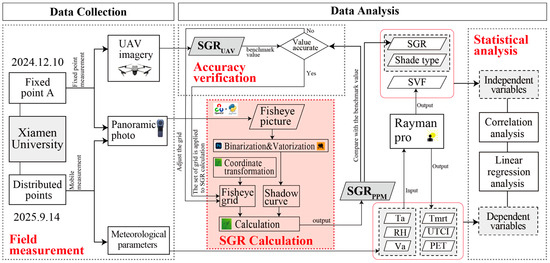
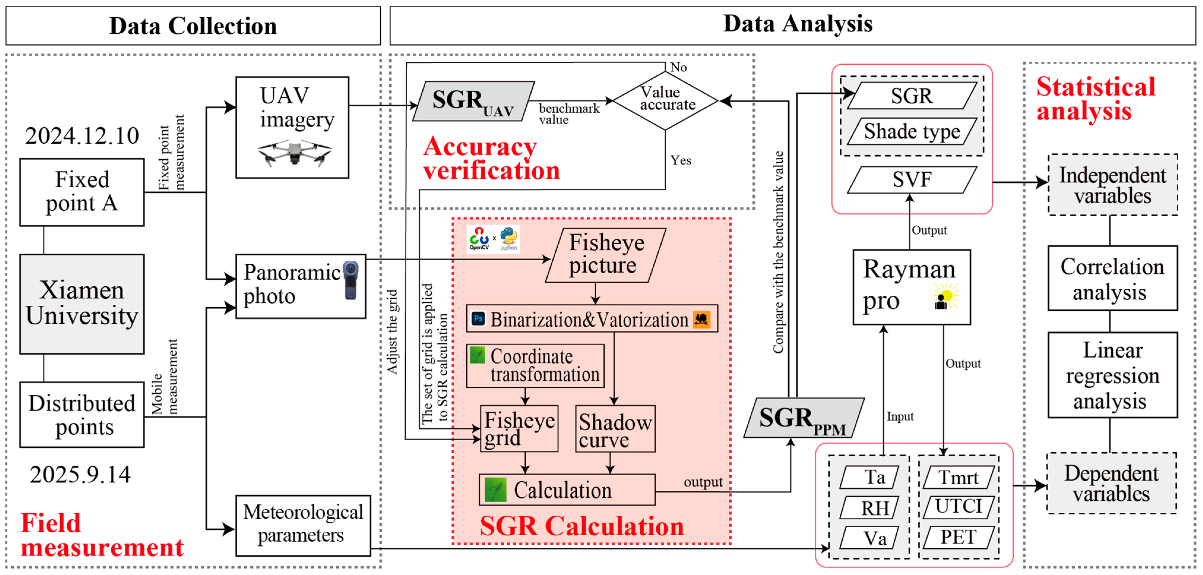
This section begins by introducing the SGR concept and the core PPM procedure. The subsequent empirical research, conducted on the campus of Xiamen University, consists of two primary phases: (1) a fixed-point measurement to verify the accuracy of the PPM framework, and (2) a mobile measurement to gather shadow and thermal environment variables for systematic analysis. There is a specific focus on calculating SGR values and thermal comfort indices for all mobile measurement points. Finally, statistical analyses are conducted to quantify the interplay between shadow and thermal conditions. The overall research workflow is shown in Figure 1, with detailed specifications provided below.
Figure 1.
Research process diagram.
2.1. Shadow Geographical Ratio (SGR)
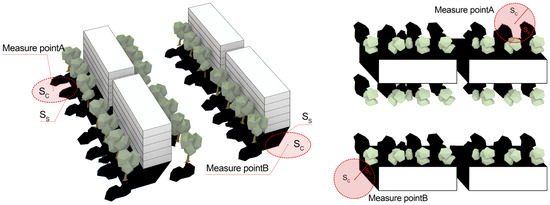
The shadow geographical ratio (SGR) is defined as the proportion of shadow-covered area within a circular sampling zone of a fixed radius, centered on a ground-level measurement point. Its values are normalized, ranging from 0 to 1 (Equation (1)).
where SS denotes the shadow area within the sampling circle, and SC denotes the area of the circle.
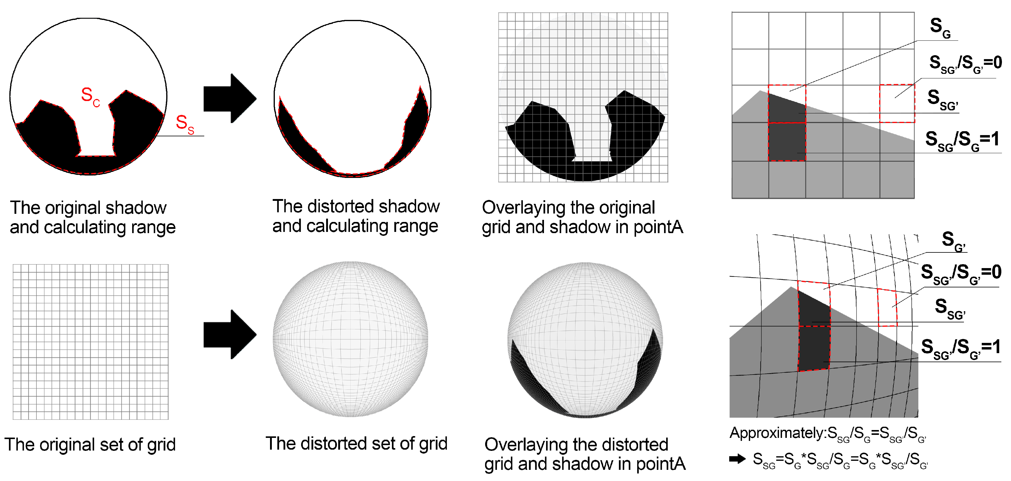
Since shadow distributions fluctuate continuously throughout the day, the SGR for each site is operationalized as the temporal average of hourly shadow ratios from sunrise to sunset (SGRti). This time-integrated approach ensures a representative characterization of the local shading conditions. The conception is illustrated in Figure 2.
Figure 2.
SGR concept illustration.
The SGR concept builds on the BSGR proposed in our previous work [15], defined as the ratio of building shadow area to the total area within a circular region centered on a certain point. SGR incorporates not only shadows cast by buildings, but also those produced by other shadow-casting elements, especially trees. This refinement is crucial for precisely assessing microclimate in densely vegetated urban fabrics, including campuses, urban blocks, and parks.
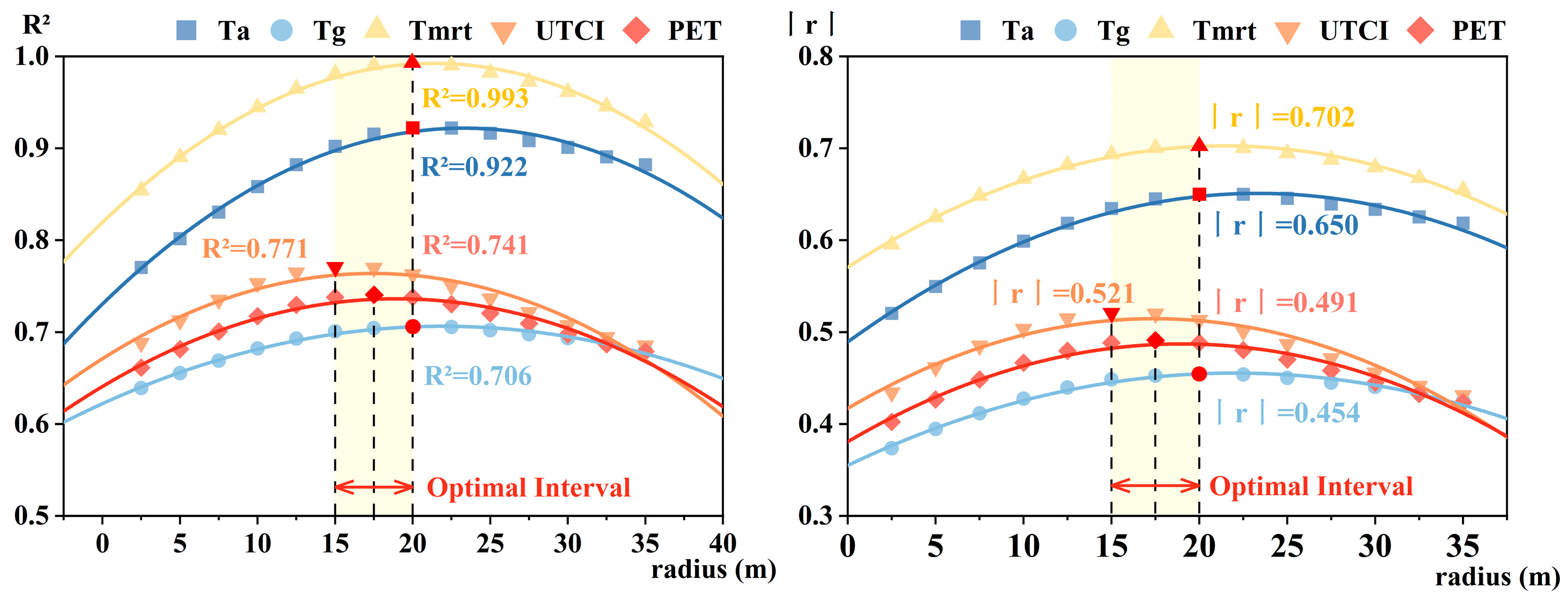
Since SGR is derived from a circular sampling zone, its value is contingent upon the selected radius, which subsequently affects the relationship of the metric with the thermal environment and comfort metrics. In the determination of BSGR in our previous study, a quadratic trend was identified between the calculation radius and its statistical significance: the correlation initially intensified before diminishing, reaching an optimum between 15 and 20 m for thermal environmental indicators. Appendix A provides the correlation between BSGR and UTCI under varying conditions (Figure A1) [15]. Accounting for the camera’s field of view and the on-site spatial constraints, the SGR calculation radius in this study was set at 10 m as a practical compromise between measurement feasibility and accuracy; this setting, although it did not perform best, made sense. If a larger calculation radius had been employed in this study, the accuracy of calculated SGR would have been diminished due to the over-compressed pixels towards the peripheral part of the fisheye images.
2.2. Panoramic Photo-Based Measurement (PPM)
The PPM framework utilizes a panoramic camera to capture real-time shadow conditions at specific locations. The resulting high-resolution images are used to calculate shadow-covered areas and, in turn, derive SGR values. The PPM workflow follows a three-stage technical progression: First, panoramic images are processed into vectorized graphics in which shadow contours can be identified. Second, an analysis grid based on the equidistant projection model is established for the fisheye imagery, which is a very crucial step that compensates for radial distortion during area calculations. Third, the identified shadow regions in the images are overlaid onto this grid, where the final shadow ratio is derived by aggregating the weighted shadow proportions within each grid cell. Each step is described in detail below.
2.2.1. Image Processing
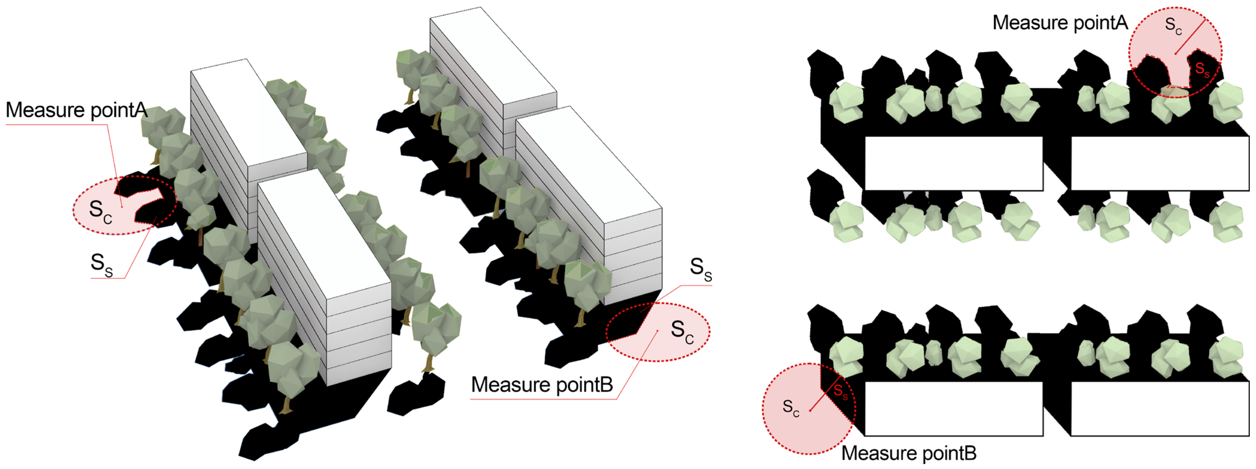
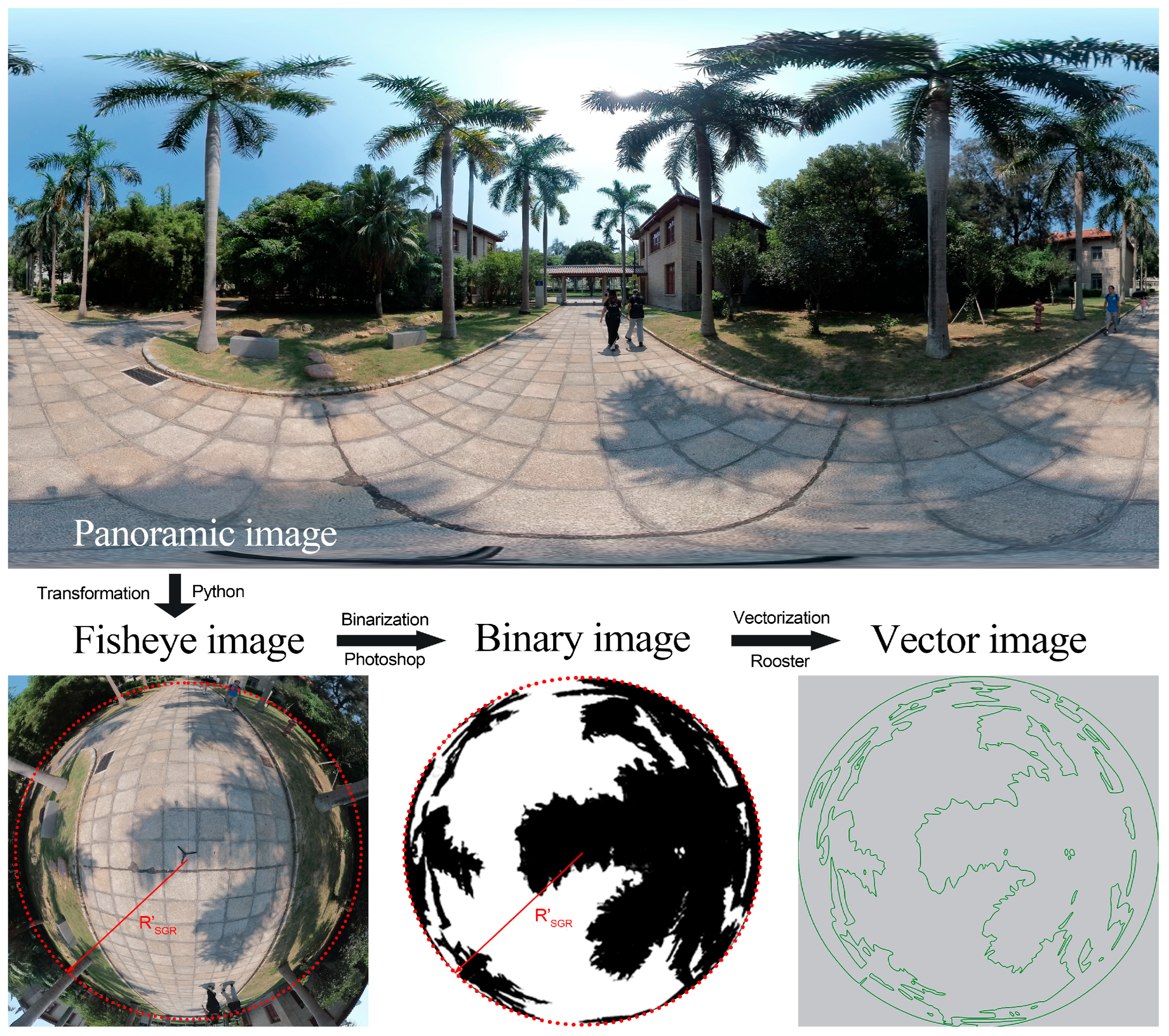
Image processing involves four steps (Figure 3)—image conversion, geometric calibration, binarization, and vectorization—that convert panoramic photographs captured on-site into vectorized shadow boundaries suitable for quantitative analysis.
Figure 3.
Panoramic image processing.
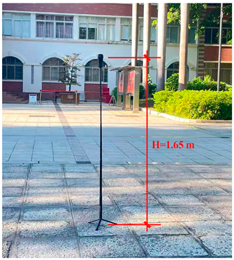
The image conversion step uses Python (Python 3.13.3) and OpenCV (4.11.0.86) to transform cylindrical panoramic photos into fisheye images via an azimuthal equidistant projection [38]. Each panoramic photo is split into upper and lower halves: the upward-facing part calculates SVF, and the downward-facing part calculates SGR. Geometric calibration defines a 10 m radius circular area on the fisheye image using an on-site reference object, and redundant portions are cropped; the fixed camera height allows this calibrated area to be reused across all measurement points. Binarization in Photoshop (Photoshop 24.0.1.112) converts downward-facing fisheye images into black-and-white pixels, where black pixels denote shadow, and any building footprint inside the circular area is excluded from the SGR calculation. Vectorization extracts shadow boundaries from binarized images using Grasshopper’s Rooster plugin (Grasshopper 1.0.0008 included with Rhino 8.13, Rooster 1.0.3.0) and converts them into closed vector curves that represent the exact geometries of the shadow regions. The detailed procedures for image processing are provided in Appendix B: Table A1.
2.2.2. Grid Establishment
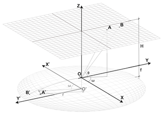
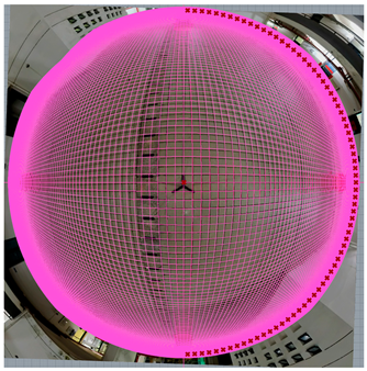
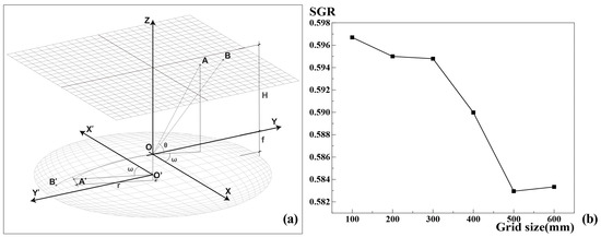
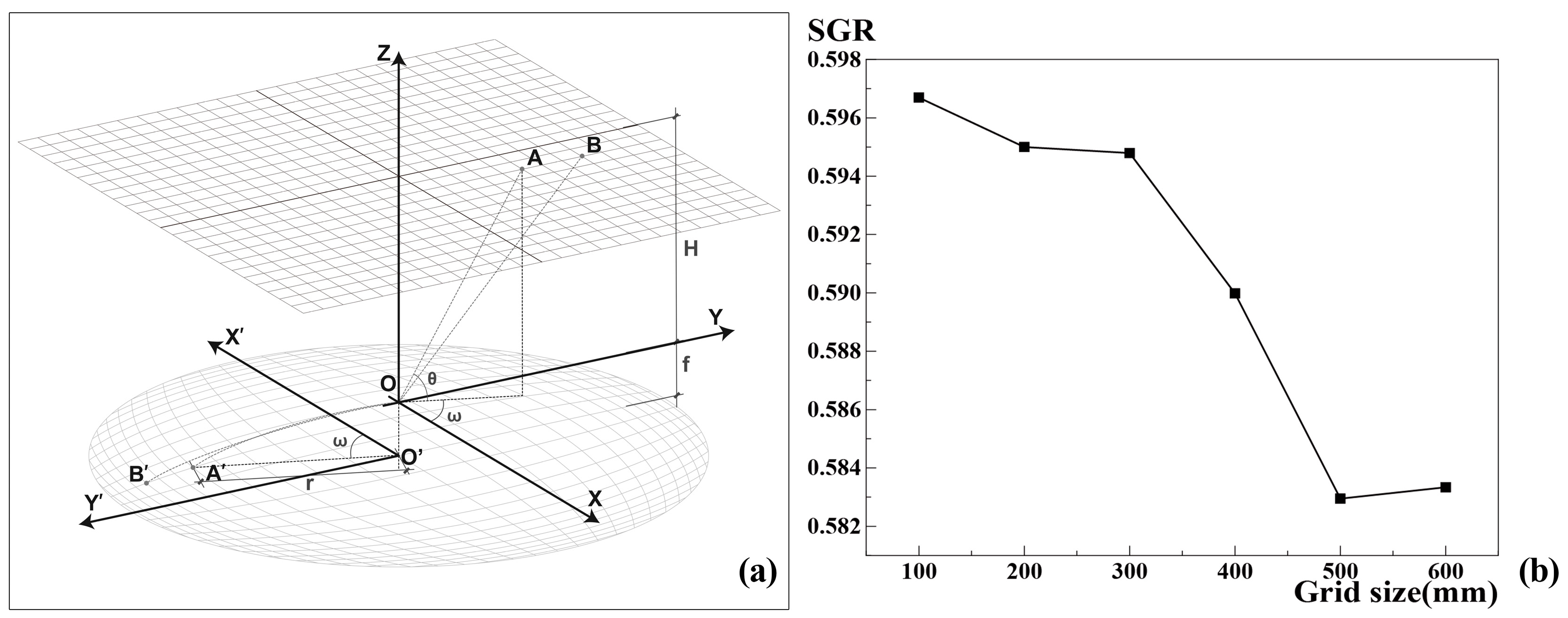
Prior to calculation, a regularly distributed set of grids in the world coordinate system is projected onto the fisheye image plane based on the equidistant projection model of the fisheye lens (Figure 4a), generating a nonlinear analytical grid that mirrors the image distortion. By establishing a special mapping between world coordinates and image pixels, this grid serves as a geometric bridge, enabling the rectification of distorted pixel areas into accurate physical shadow areas. The specific parameter settings and operating procedure for the grid establishment are detailed in Appendix B: Table A2. The underlying geometric principles and the governing equation are detailed in Equation (2).
where r represents the distance between a point in the image and the distortion center; f is the focal length of the fisheye camera; and θ is the angle between the incident ray and the optical axis, that is, the incident angle.
Figure 4.
Diagram of equidistant projection model (a), and the result of grid independence analysis (b).
To ensure a reasonable balance between computational accuracy and efficiency in calculations, a grid-independence test was first performed by comparing SGR values calculated with grid sizes of 10, 20, 30, 40, and 50 cm, to decide an appropriate grid size. The results indicated that when the grid size was 30 cm or smaller, the SGR values calculated changed little with different grid sizes (Figure 4b). Therefore, a grid size of 30 cm × 30 cm was selected for subsequent analysis.
2.2.3. SGR Calculation
The calculation of SGR is a segment following data collection, and belongs to the data processing and analysis part. It outputs the proposed shadow indicator SGR and is an essential component of the overall PPM framework. Placing it here rather than in Section 2.4 (Data processing and analysis) maintains the coherence and completeness of the PPM framework description.
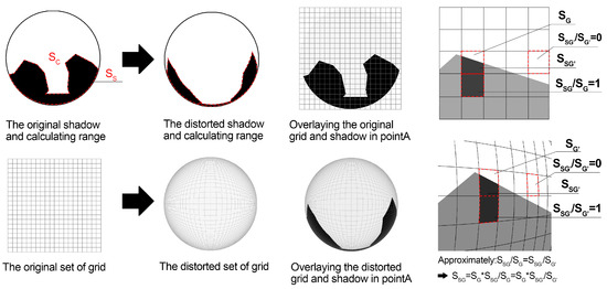
The calculation of shadow area is based on grid overlay and integration. First, the vectorized shadow boundary curves are imported into the Grasshopper platform (Grasshopper 1.0.0008 included with Rhino 8.13) and spatially registered with the 10 m radius analytical grids, ensuring that the image periphery coincides with the computational boundary. Each grid cell is then computed individually to determine the proportion of its area covered by shadow, from which the shadow area in that cell is obtained (actual cell area × shadow proportion). The total shadow area within the calculation range is obtained by summing the shadow areas of all cells. Using this method, SGR values are calculated for each image. The schematic diagram (Figure 5) and the corresponding formula (Equation (3)) are provided below:
where SS represents the shadow area within the sampling circle, SC represents the area of the sampling circle, denotes the shadow area within the i-th grid cell before distortion, denotes the area of the i-th grid cell before distortion, refers to the shadow area within the i-th grid cell after distortion, and refers to the area of the i-th grid cell after distortion.
Figure 5.
Grid overlaying and calculation.
2.3. Field Measurement
2.3.1. Study Area
Xiamen (24.4801069° N, 118.0853479° E), located on China’s southeastern coast, has a subtropical maritime monsoon climate characterized by high humidity and intense solar radiation. The area’s climate profile is defined by prolonged, sweltering summers, with a mean annual temperature of 20.9 °C. Monthly averages peak in July at 28.4 °C and reach a minimum, in January, of 12.5 °C. Xiamen University, situated in the city’s urban core, contains a diverse mix of buildings and vegetation, giving rise to a wide range of shadow conditions. A representative teaching area on campus was selected as the study site; it was predominantly composed of academic buildings and a library, with building heights ranging from 2 to 7 stories, as well as dense vegetation and a lake. The selected area contains a varied spatial structure, with buildings enclosing a series of outdoor spaces, from open plazas and courtyards to narrow passageways. Building and tree shadows alternate and overlap across the site, creating composite shadow zones that vary in duration and spatial pattern over time.
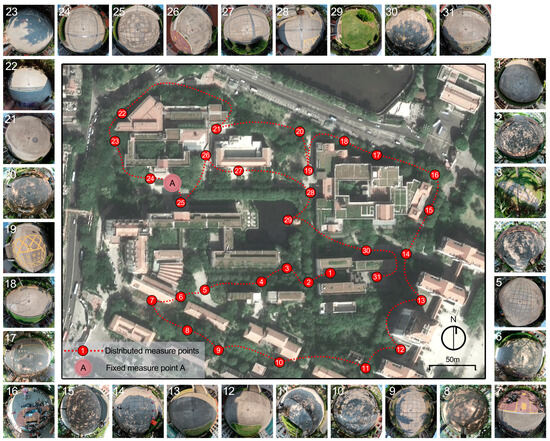
The field measurement in this study included two components: fixed-point measurement and mobile measurement (Table 1). The former were used to assess the accuracy of the PPM, and the latter to examine the relationship between shadow and thermal environment. Measurement points were selected based on two criteria: practical feasibility in the field and spatial representativeness, ensuring the inclusion of a diverse spectrum of shading configurations (Figure 6).
Table 1.
Experimental setup and measurement objectives.
Figure 6.
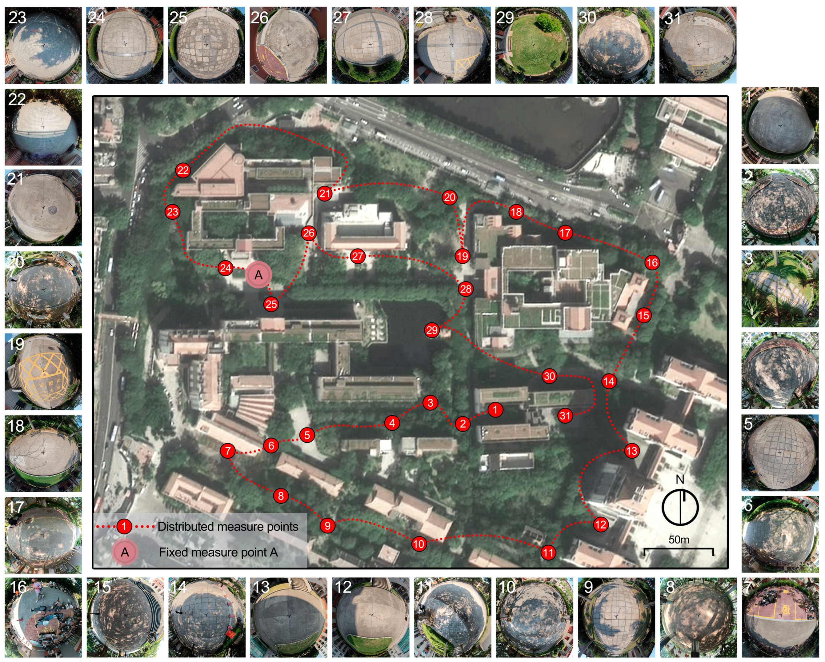
Measurement point location and ground perspective fisheye image at 12:00.
For the fixed-point validation, in which UAV imagery served as the benchmark for validating shadow ratio, the site had to be in an open area free of overhead obstructions such as tree canopies or umbrellas. The square in front of the College of Economics was designated as fixed measurement point A. This site provided an ideal testing ground, as it transitions through a complex sequence of building and tree shadows throughout the day, offering a rigorous environment for verifying the PPM’s reliability. For mobile measurement, 31 points were selected across the campus, with distance, route, spatial typology, and usage frequency considered. These points included sidewalks, rest areas with seating, building-front plazas, and shaded spaces beneath trees, ensuring a comprehensive dataset of diverse shading and spatial conditions.
2.3.2. Fixed-Point Measurement
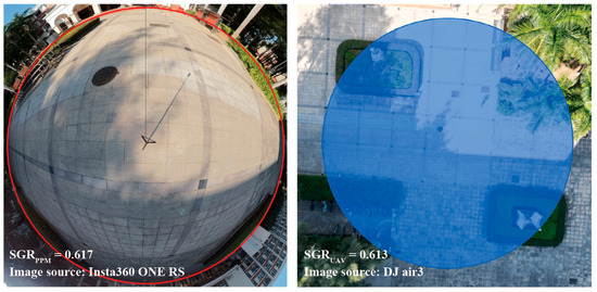
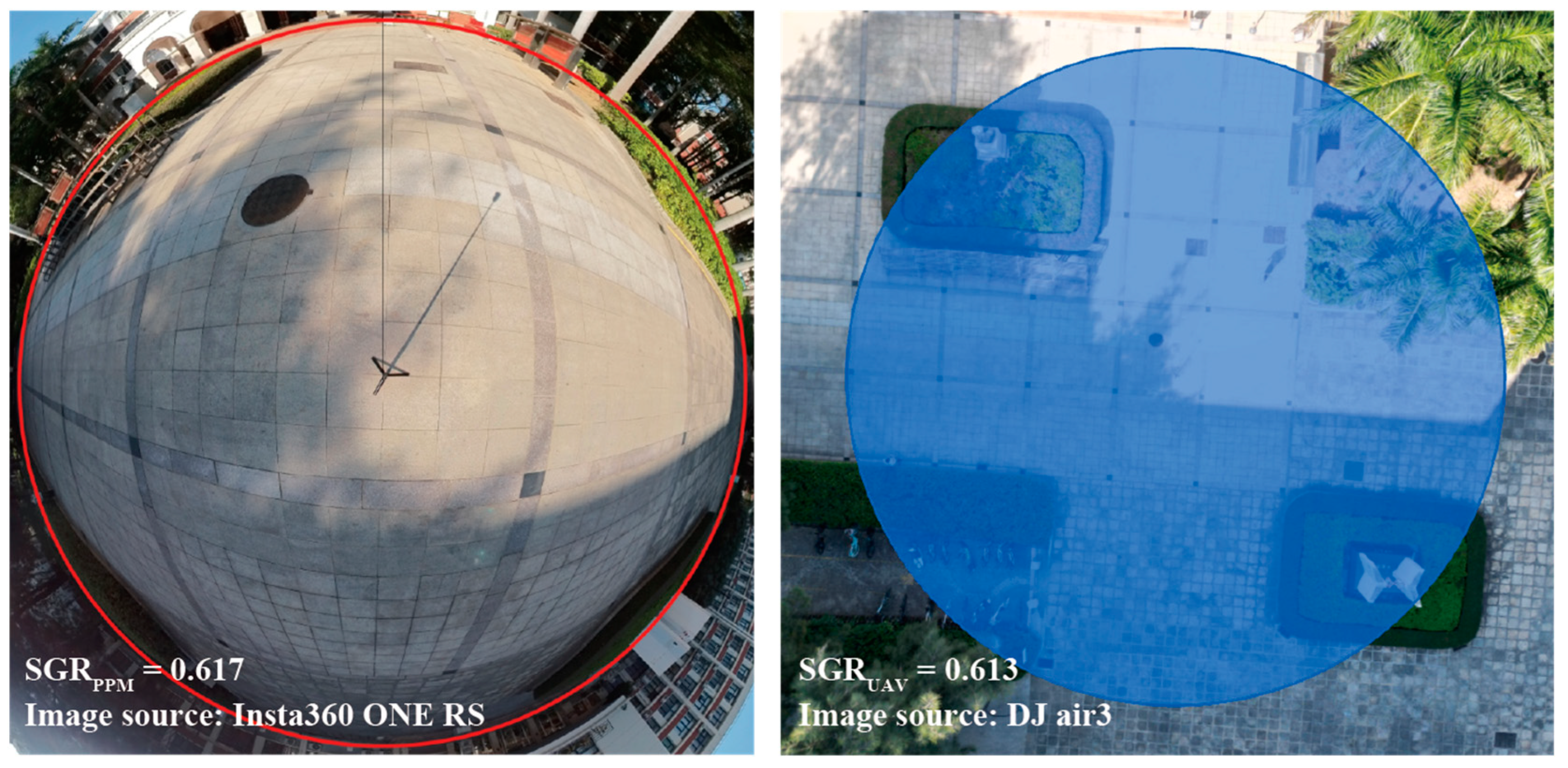
To validate the measurement accuracy of PPM, a comparative analysis was conducted at Fixed point A on 10 December 2024, using both PPM and UAV-based methods, with a 10 m calculation radius. Figure 7 shows the panoramic photo and UAV imagery taken at the same time and location. The operational procedures and parameter settings for the two methods were as follows.
Figure 7.
Comparison of SGR calculation derived from PPM (left) and UAV (right). The circle (left) and blue area (right) indicate the 10 m radius zones delineated based on field calibration.
- PPM method: A panoramic camera (Insta360 ONE RS, Arashi Vision Inc., Shenzhen, Guangdong, China) was deployed at a height of 1.65 m to capture imagery at 10 min intervals from 10:00 to 15:00. Following the computational workflow delineated in Section 2.2, SGRPPM values for each temporal sample were calculated.
- UAV method: A drone (DJI Air 3, DJI, Shenzhen, Guangdong, China) was used to capture overhead images of the site at the same time intervals. Given the high shooting altitude, these images functioned as approximate orthographic projections, enabling direct spatial quantification. The UAV imageries were then binarized in Photoshop, and SGRUAV values for each temporal sample were computed using the area calculation module in Grasshopper.
A total of 30 synchronized image pairs were collected. Taking SGRUAV as the benchmark, the accuracy and reliability of the PPM framework were evaluated by statistically analyzing its cross-method consistency with SGRPPM. Even obtained in the same site, the shadows captured at each of the 30 time points are all distinct in shadow morphology and shadow area due to the continuously changing solar altitude and solar azimuth. Thus, these 30 independent instances serve as separate samples for accuracy assessment.
The fixed-point measurement was dedicated solely to methodological validation and remained independent of the thermal environment analysis. The objectives being verified in this stage included the following three parts: whether the panoramic camera captured the current shadow with complex morphology clearly, whether the image processing was credible and whether the calculated value of PPM aligned with that of the benchmark value. Subsequently, it was determined that the use of winter data for this calibration phase did not influence the subsequent hot-season mobile measurement findings.
2.3.3. Mobile Measurement Across Distributed Points
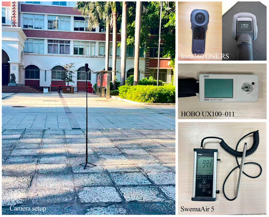
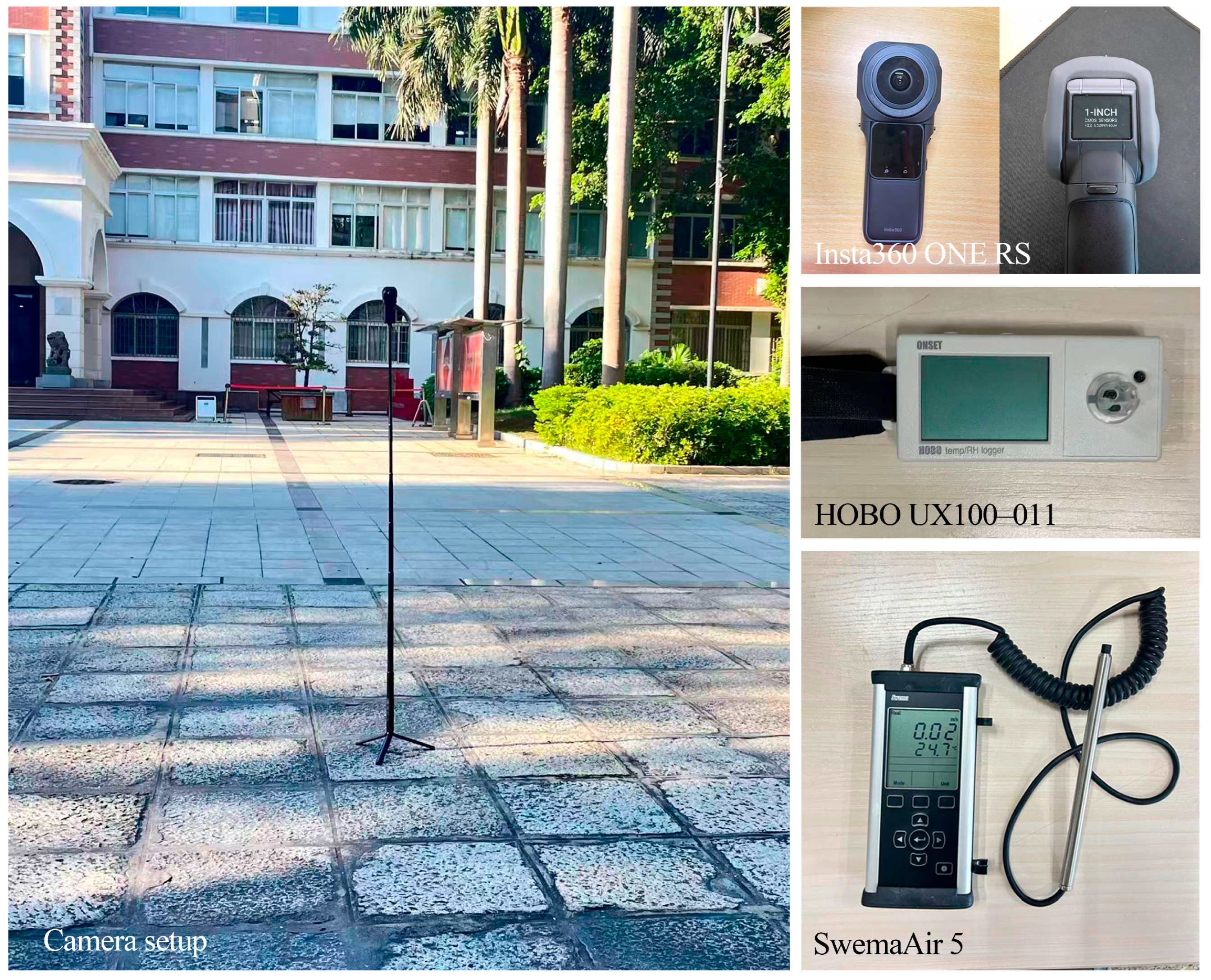
Following the PPM accuracy validation, field measurement of SGR, SVF, and thermal environment parameters was conducted at 31 points across the Xiamen University campus from 6:00 to 18:00 on 14 September 2025. The meteorological conditions were predominantly clear and cloudless, except for brief intermittent cloud cover for approximately 30 min around 9:00. Adopting a mobile transect approach, the research team traversed a standardized route once per hour, passing through all measurement points to take panoramic photographs and record climatic variables, including Ta, RH, and Va. A total of 12 measurement rounds were completed during the day. The field measurement instruments are shown in Figure 8.
Figure 8.
Panoramic camera setup and thermal environment measurement instruments.
This mobile measurement design is appropriate for demonstrating the practical utility of the PPM framework and for collecting shadow–thermal relationship data. Testing the PPM framework in a real, complex campus environment required covering a sufficient number of points with diverse spatial morphologies, allowing the collection of varied shading conditions and corresponding thermal parameters to support subsequent regression analysis. Moreover, the fixed-route and fixed-interval cycling ensured that all points were compared under similar meteorological conditions.
1. SGR and SVF measurement: A total of 372 panoramic photographs (31 points × 12 rounds) were collected. Using OpenCV in Python, these photographs were converted into two fisheye views: a downward-facing view of the ground and an upward-facing view of the sky [38]. The downward-facing fisheye images were used to calculate SGR at each point based on the PPM method. The upward-facing fisheye images were used to calculate SVF at each point. Specifically, the upward-facing fisheye images were binarized and then imported into Rayman Pro 3.1 software, which computed and recorded the SVF values.
2. Ta, RH, and Va measurement: At the start of each round, the research team departed from point 1 carrying a temperature–humidity logger (Hobo Ware) and an anemometer and then proceeded sequentially through points 2 to 31. The instruments had been calibrated beforehand. Throughout the survey, they were held 1.1 m above the ground, with the probes oriented in the direction of travel. Upon reaching each measurement point, the time was recorded and the team remained there for 30 s. The temperature–humidity logger recorded data simultaneously at 1 s intervals. For the anemometer, once its reading had stabilized, five measurements were taken at 1 s intervals and averaged as the Va for that point at that time. To account for instrument adjustment to ambient conditions, the first 10 s and last 5 s of each 30 s period were excluded from the analysis. Only the values recorded during the middle 15 s, when the instruments were stationary, were retained and averaged. Table 2 lists the main technical parameters of the sensors.
Table 2.
Technical specifications of the measurement instruments.
3. Tmrt, PET, and UTCI calculations: To comprehensively evaluate the relationship between shadow and thermal comfort, Tmrt, PET, and UTCI were calculated for each point from field data. Tmrt quantifies the radiative heat exchange between a human body and its surroundings, linking SGR to thermal comfort. PET [39] converts outdoor thermal stress to an equivalent indoor temperature via human energy balance. UTCI [40] provides a biometeorological perspective, capturing integrated physiological strain under dynamic climatic conditions.
Conventional high-precision Tmrt measurement methods, such as black globe thermometers and six-directional radiometers, are widely used for assessing the thermal environment. However, these approaches either require sufficient stabilization time, or involve complex equipment setups that are less feasible for rapid mobile surveys. Due to the mobile measurement design, the effective dwell time at each point was only about 1 min, which is insufficient for black globe thermometers or six-directional radiometers to reach thermal equilibrium. Such requirements are difficult to satisfy in mobile transect surveys with high spatial density and tight temporal constraints. Extending the dwell time would substantially increase the duration of each measurement round, leading to larger errors in subsequent temporal interpolation and reducing the number of effective rounds per day. Recent advancements have introduced alternative approaches, such as the PanoMRT model, which estimates Tmrt from 360° thermal panoramas that capture pedestrian-level surface temperatures [41]. This method, while effective, still requires a considerable amount of time per location, limiting its use in rapid, multi-point mobile surveys.
Given these practical constraints, we adopted the RayMan model for Tmrt (Equations (4) and (5)) and the PET calculations in this study. RayMan accepts inputs that can be rapidly collected within our pre-defined dwell time per site, including Ta, RH, Va, and fisheye images. Its computational efficiency allows for batch processing of multiple sites, enabling us to complete full transect rounds within a limited time window and ensuring that all measurement points within a given round are exposed to comparable meteorological conditions [42,43]. Based on the Tmrt outputs, UTCI values were further calculated following Equation (6).
where denotes the Stefan–Boltzmann constant (5.67 × 10⁻⁸ W·m−2·K−4), denotes the emission coefficient of human body, with a standard value of 0.97. denotes the combined contribution of diffuse solar radiation and diffusely reflected global radiation. is the short-wave absorption coefficient of the exposed body surface, and its standard value is 0.7. denotes the solar radiation intensity on a surface oriented perpendicular to the direction of the incoming radiation, while the surface projection factor depends on both the radiation direction and body posture.
where V10 represents the air velocity at a height of 10 m and Va represents the air velocity at the height of 1.1 m recorded by the anemometer.
2.4. Data Processing and Analysis
2.4.1. Temporal Alignment
Owing to the asynchronous nature of the mobile transect method, measurements across the 31 sites were captured at varying intervals within each hourly cycle. To facilitate a rigorous cross-site comparison at standardized intervals, it was necessary to synchronize all observations to a common temporal reference. In this study, cubic spline interpolation was employed to transform the data series for all points to precise hourly increments from 6:00 to 18:00. Cubic spline interpolation constructs a smooth curve by fitting piecewise cubic polynomials, ensuring that adjacent segments maintain continuous function values and derivatives at their junctions. Such high-order smoothness is well suited to continuously varying environmental variables like temperature and humidity, preserving the overall trend while avoiding the jagged artifacts that are typical of linear interpolation. The interpolation process was implemented in Python using the scipy.interpolate. CubicSpline function [44]. To mitigate potential edge–point overshoot, the initial and terminal data points were truncated, retaining only the robust interpolated values for final analysis.
2.4.2. Accuracy Verification
The RMSE and MRE were employed as evaluation metrics to quantify the accuracy of the PPM in this study. RMSE reflects the average absolute deviation between calculated and measured values, while MRE reflects the average percentage error relative to the measured values. Together, these two metrics provide a comprehensive assessment of the method’s precision. To evaluate the calculation accuracy of the PPM-derived SGR values, two corresponding sets of SGR values were respectively obtained from UAV imagery and PPM. RMSE and MRE were then calculated using Equations (8) and (9) for these paired values to objectively assess the reliability of PPM measurement.
2.4.3. Statistical Analysis
To examine the relationship between shadow and the thermal environment, correlation analysis and linear regression analysis were employed in this study.
1. Pearson correlation analysis. The Pearson correlation coefficient (r) was calculated to assess the strength and direction of the linear relationships between SGR and SVF, on the one hand, and thermal environmental parameters and thermal comfort indices, on the other. The closer the absolute value of r is to 1, the stronger the linear association between the two variables. The coefficient of determination (r2) further indicates the proportion of variance in one variable that can be explained by the other, with values closer to 1 indicating greater shared variance between the two variables. All correlation analyses were conducted in SPSS 27.0.1.0.0, where Pearson correlation coefficients and their corresponding significance levels (p) were obtained to evaluate the statistical associations between shadow and the thermal environment.
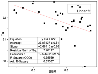
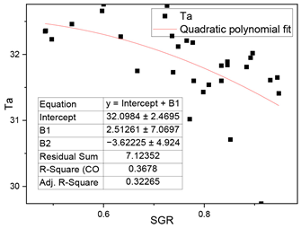
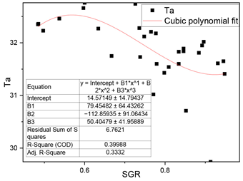
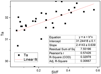
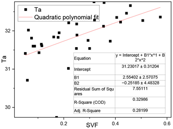
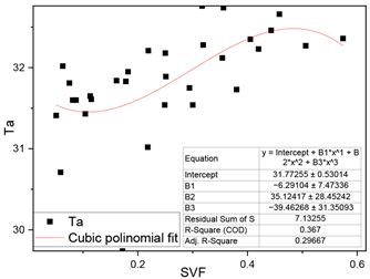
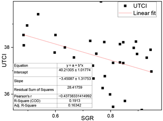
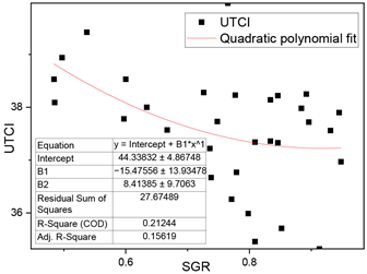
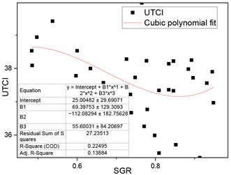
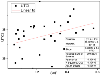
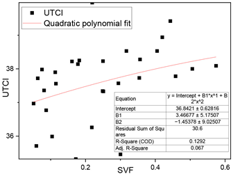
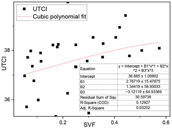
2. Linear regression analysis. To quantify the extent to which shadow influences the thermal environment, linear regression was employed to construct statistical models. Scatterplots, residual analyses, and statistical tests were employed to confirm that the data met the underlying assumptions of the model. In addition, several nonlinear models, including polynomial and logarithmic regressions between two shadow indicators (SVF, SGR) and Ta, UTCI, were also tested in advance. The goodness of fit and residual distributions across the successfully fitted models were compared, and the result showed that linear regression provided the best overall fit. The detailed data of this test were provided in Appendix C. Based on this, a series of linear regression models were constructed, with SGR and SVF as predictor variables and thermal environment and comfort parameters (Ta, Tmrt, PET, UTCI, etc.) as response variables. The model’s fitness was evaluated using the coefficient of determination (R2), which ranges from 0 to 1, and the sensitivity of the dependent variable to the independent variable was evaluated using standard regression coefficients (B).
3. Results
3.1. PPM Accuracy Validation Results
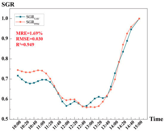
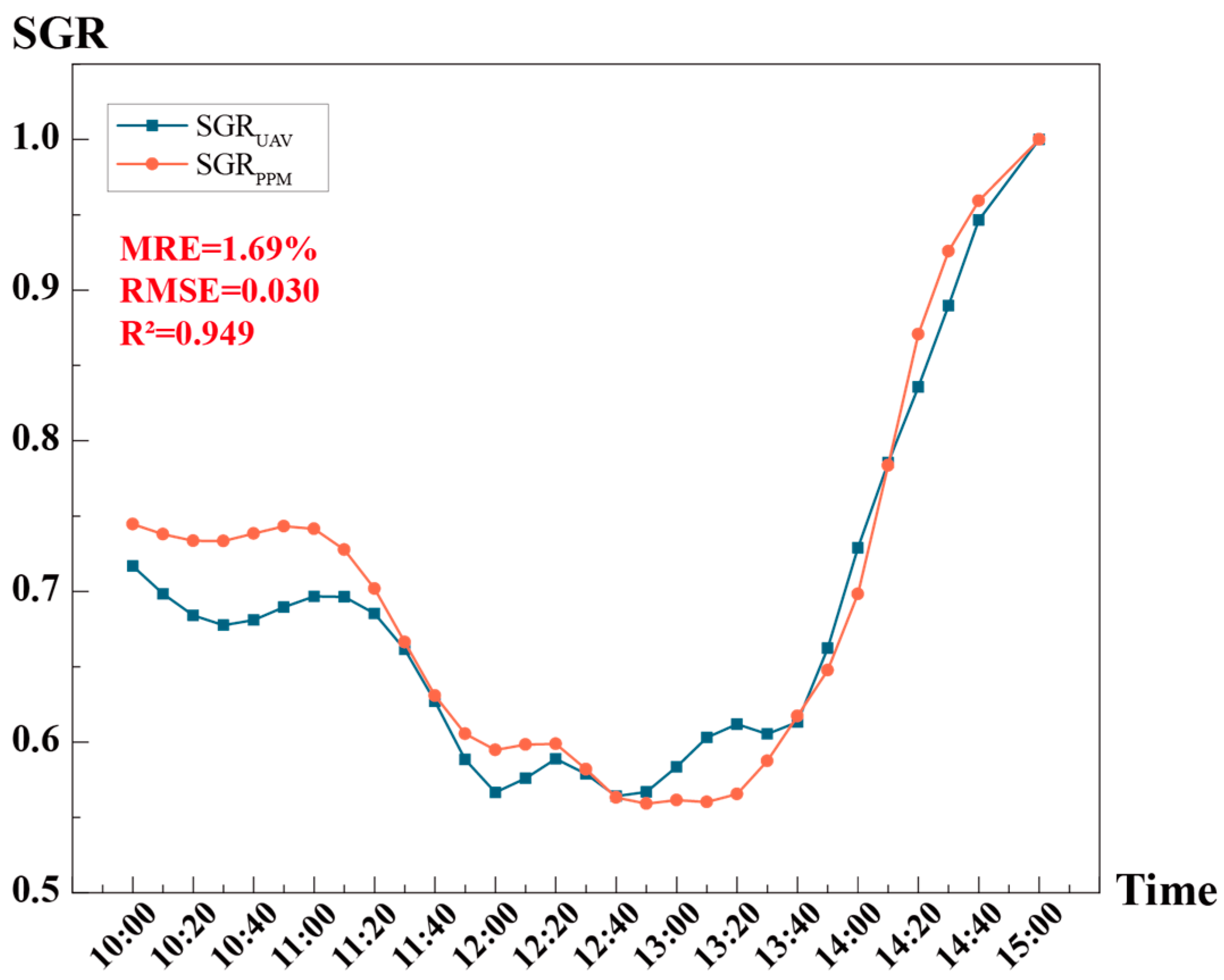
The accuracy validation results are presented in Figure 9 and Table 3, demonstrating high congruence between the PPM-derived SGR (SGRPPM) and the UAV-based benchmarks (SGRUAV). Across the 30 temporal samples, the absolute relative error ranged from a maximum of 8.42% to a minimum of 0.177% (the measurement at 15:00 was excluded from comparison, as the area was fully covered by shadow with both SGR values at 1). Notably, 73.33% (22/30) of the observations showed absolute relative errors below 5%; 46.67% (14/30) below 3%; and 23.33% (7/30) below 1%. Furthermore, the scatterplot illustrates a strong linear correspondence and significant overlap between the two datasets, supported by low aggregate error metrics and a robust correlation coefficient (RMSE = 0.03, MRE = 1.69%, R2 = 0.949). These results confirm that PPM provides accurate field estimates of SGR and is applicable in subsequent analysis.
Figure 9.
Comparison of SGR values from the PPM and UAV methods.
Table 3.
Comparison of SGR values and relative errors from the PPM and UAV methods.
3.2. Descriptive Statistics of Shadows and Thermal Indicators
Table 4 summarizes the descriptive statistics for mobile measurement sites and Table 5 illustrates feature points and spatial morphologies documented by upward-facing fisheye images. In this analysis, the maximum SGR is defined as the highest SGRti value observed within a measurement round, excluding saturated values of 1.0. Values of 1 were excluded because they represented fully shaded conditions that occurred across all points and therefore did not help to distinguish spatial differences among measurement locations. The dataset reveals a mean SGR of 0.795 (SD = 0.121), suggesting an environment characterized by extensive shadow coverage, with moderate spatial fluctuations. The maximum SGR value of 0.974 occurred at point 17 (a campus road between the library’s north facade and an adjacent wall), while the minimum value of 0.494 occurred at point 27 (a plaza south of a three-story teaching building). Notably, point 17 also recorded the minimum SVF (0.051), whereas the maximum SVF (0.574) was found at point 29 (an open green space by the lake). This inverse correlation at point 17 highlights the synergistic shading effects of structural massing to the south and dense vegetative canopies to the north.
Table 4.
Summary of measured values of all 31 measured points. Bold font in the table footer indicates summary statistics (mean, standard deviation, and maximum).
Table 5.
Shadows and environmental features of typical points.
Thermal environment and comfort indicators exhibited pronounced spatial heterogeneity across the study site. Daily mean Ta ranged from 29.74 °C to 32.76 °C, peaking at point 31 (a southern academic plaza) and reaching its minimum at point 1 (a northern atrium). RH showed limited variation, with a mean value of 73.45%, indicating relatively minor spatial differences across the site. Va displayed the highest degree of fluctuation (SD = 0.24 m/s), reflecting localized aerodynamic diversities. Across the 31 points, the daily mean values of Tmrt, PET, and UTCI were 47.72 °C, 40.13 °C, and 37.59 °C, respectively. Notably, point 7 (a bicycle parking area) was the most thermally stressed location, recording the maxima for all three indicators (Tmrt = 52.37 °C, PET = 43.76 °C, UTCI = 39.97 °C). Conversely, the lowest Tmrt and PET were observed at point 2 (a tree-shaded road intersection), while the minimum UTCI aligned with Ta minimum at point 1. The substantial spatial ranges of Tmrt (8.48 °C), PET (6.35 °C), and UTCI (4.65 °C) underscore the significant influence of site-specific radiative conditions on pedestrian comfort.
The 31 measurement points encompassed a broad range of outdoor space types and shadow conditions, with all recorded variables exhibiting moderate statistical dispersion. This inherent variance ensures the robustness of the dataset for subsequent statistical analyses. In the following quantitative analyses, unless otherwise specified, the thermal environment and comfort indicators for each point are represented by their daily mean values.
3.3. Relationships Among Shadow Indicators, Thermal Environment and Thermal Comfort Parameters
3.3.1. Relationship Between SGR and SVF
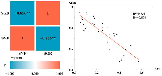
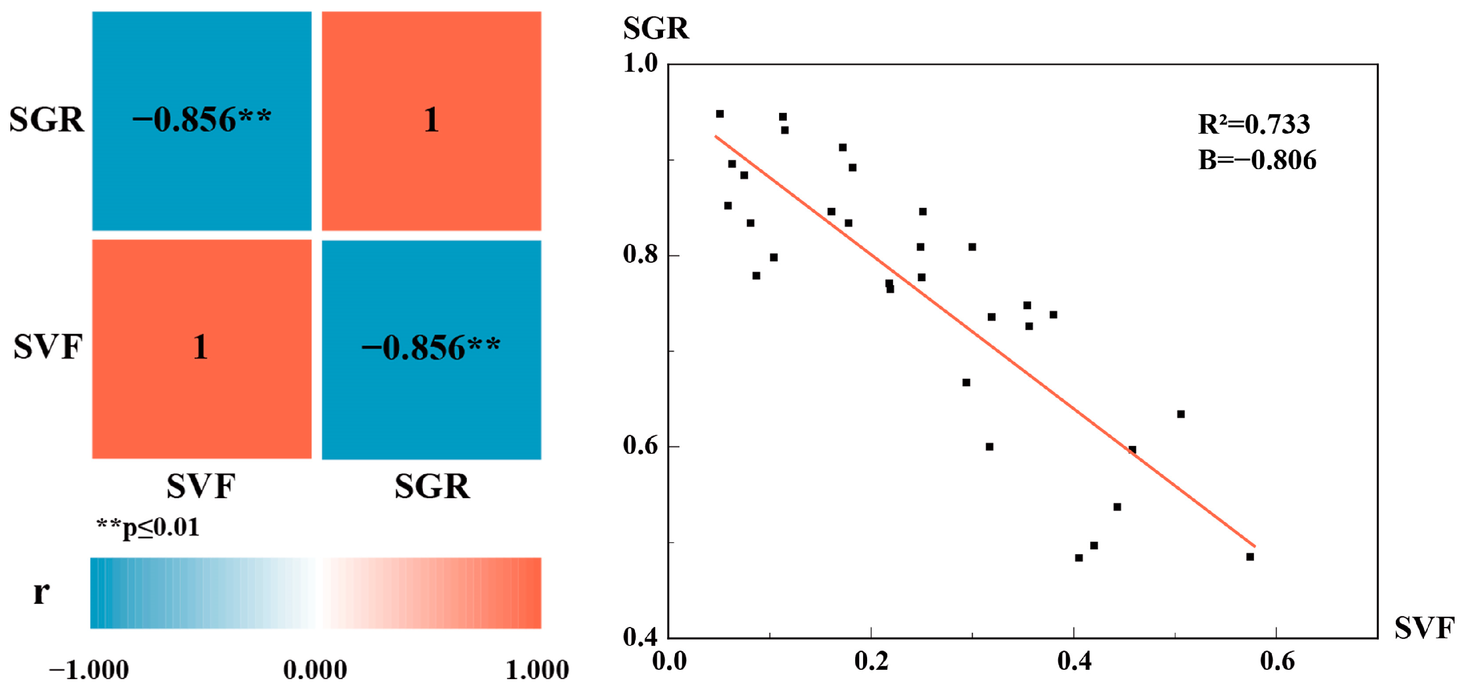
Correlation analysis showed a strong negative correlation between SGR and SVF (r = −0.856). Regression analysis further indicated a significant negative linear relationship between the two variables (R2 = 0.733, Figure 10). For a given measurement point, a lower SVF indicates a higher degree of sky obstruction by surrounding elements and therefore generally corresponds to greater shadow coverage.
Figure 10.
Correlation analysis (left) and linear regression analysis (right) between SGR and SVF.
3.3.2. Relationship Between Shadow Indicators and Thermal Parameters
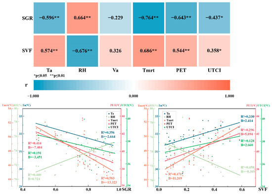
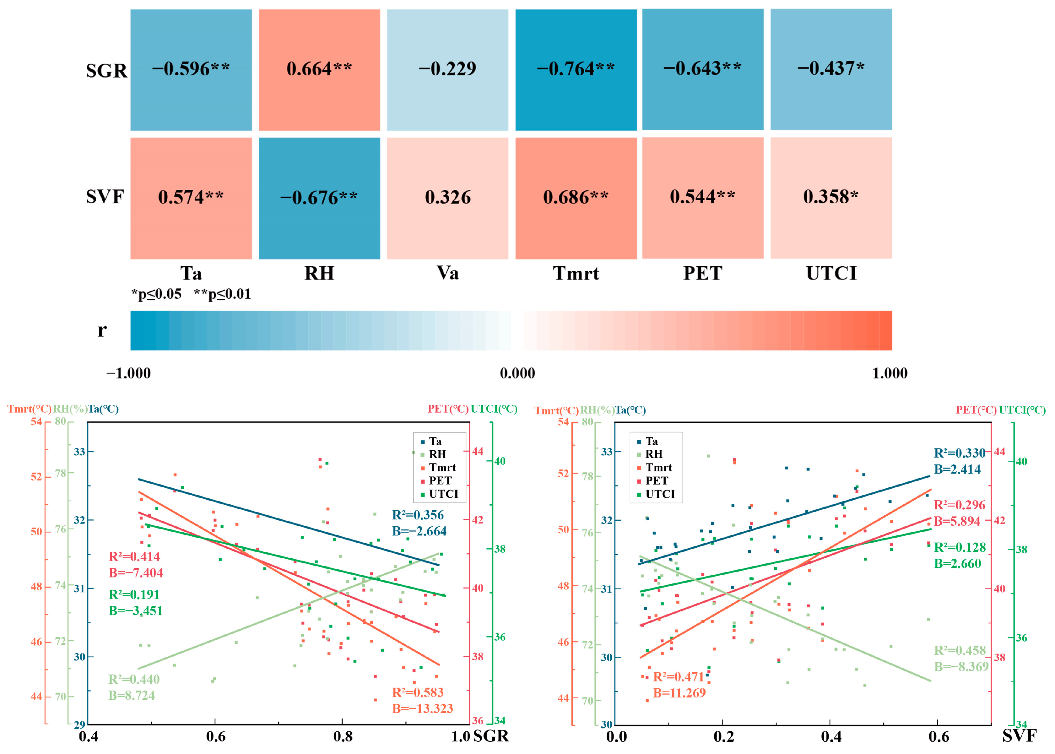
Correlation analysis between shadow and thermal environment indicators revealed that SGR and SVF were associated with different thermal parameters to different degrees (Figure 11). Specifically, SGR showed stronger correlations with Ta and Tmrt than did SVF (Pearson correlation coefficients r: −0.596 vs. 0.574 for Ta; −0.764 vs. 0.686 for Tmrt), while SVF demonstrated a stronger correlation with RH than SGR (r: −0.676 vs. 0.664). Neither SGR nor SVF showed significant correlation with Va (p > 0.05 for both).
Figure 11.
Correlation and linear regression analysis between shadow index and thermal index.
Using SGR and SVF as predictor variables and Ta, RH, and Tmrt as response variables, linear regression models were constructed. The results showed that SGR provided a better fit for Ta and Tmrt than SVF (R2: 0.356 vs. 0.330 for Ta; 0.583 vs. 0.471 for Tmrt), whereas SVF was a slightly better fit for RH than SGR (R2: 0.458 vs. 0.440). We further compared regression coefficients (B) and found that SGR exhibited steeper regression slopes for all three thermal parameters. This suggests that although correlation strengths vary, microclimatic variables are inherently more sensitive to incremental changes in SGR than in SVF. Consequently, SGR may exert a stronger influence on the thermal environment.
Correlation analysis between shadow and thermal comfort indicators showed that SGR correlated more strongly with PET and UTCI than did SVF (r: −0.643 vs. 0.544 for PET; −0.437 vs. 0.358 for UTCI). Linear regression results further demonstrated that SGR also provided a better fit for PET and UTCI relative to SVF (R2: 0.414 vs. 0.296 for PET; 0.191 vs. 0.128 for UTCI). Comparison of regression coefficients revealed that SGR had greater regression slopes for thermal comfort indicators than SVF, indicating that thermal comfort parameters are more sensitive to changes in SGR.
3.3.3. Relationship Between Shadow Indicators and Thermal Stability
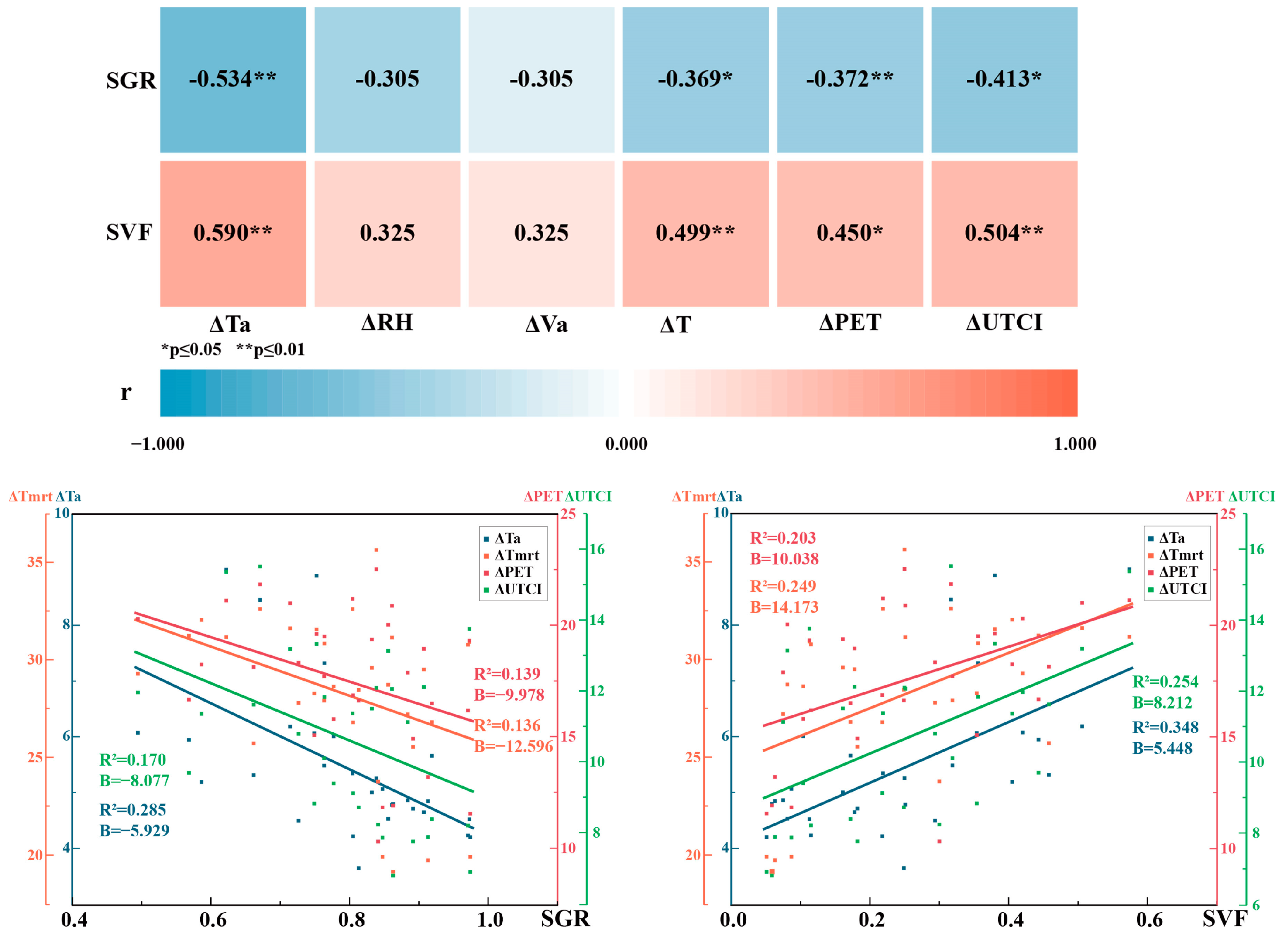
To investigate the role of shading in enhancing thermal stability, the fluctuation ranges (maximum minus minimum) of all microclimatic and comfort parameters were analyzed, denoted as ∆Ta, ∆RH, ∆V, ∆Tmrt, ∆PET, and ∆UTCI. Correlations between these fluctuation metrics and shadow indicators were assessed, followed by the construction of linear regression models with the fluctuation ranges as response variables (Figure 12).
Figure 12.
Correlation and linear regression analysis between shadow index and the fluctuation ranges of the thermal environment index.
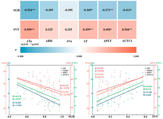
Both SGR and SVF were strongly correlated with the fluctuation ranges of Ta, Tmrt, PET, and UTCI (p < 0.01), but not with the those of RH or V (p > 0.05). Specifically, SGR negatively correlated with these fluctuation metrics, whereas SVF did so positively, with SVF demonstrating stronger correlation coefficients (r) than SGR. For ∆Ta: r = −0.534 (SGR) vs. r = 0.590 (SVF); for ∆Tmrt: r = −0.534 (SGR) vs. r = 0.499 (SVF); for ∆PET: r = −0.372 (SGR) vs. r = 0.450 (SVF); for ∆UTCI: r = −0.413 (SGR) vs. r = 0.504 (SVF). This indicates that points with lower SVF or higher SGR tended to experience smaller fluctuations in thermal indices.
Linear regression results corroborated this pattern, with SVF consistently yielding superior R2 compared to SGR when predicting fluctuation magnitudes. Specifically, for ∆Ta: R2 = 0.285 (SGR) vs. R2 = 0.348 (SVF); for ∆Tmrt: R2 = 0.136 (SGR) vs. R2 = 0.249 (SVF); for ∆PET: R2 = 0.139 (SGR) vs. R2 = 0.203 (SVF); for ∆UTCI: R2 = 0.170 (SGR) vs. R2 = 0.254 (SVF). Furthermore, the B values for SVF were also slightly larger than those for SGR for ∆Ta, ∆Tmrt, ∆PET, and ∆UTCI. These findings were consistent with the correlation analysis, confirming that shadow indicators are clearly related to thermal environment stability.
3.3.4. Spatiotemporal Effects of Shadows on Thermal Environment
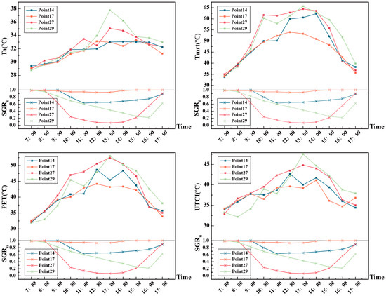
Four representative points and three typical times of day were selected to capture the spatiotemporal variations in the influence of SGR on thermal conditions, thereby providing a more direct view of how shadow affects the thermal environment.
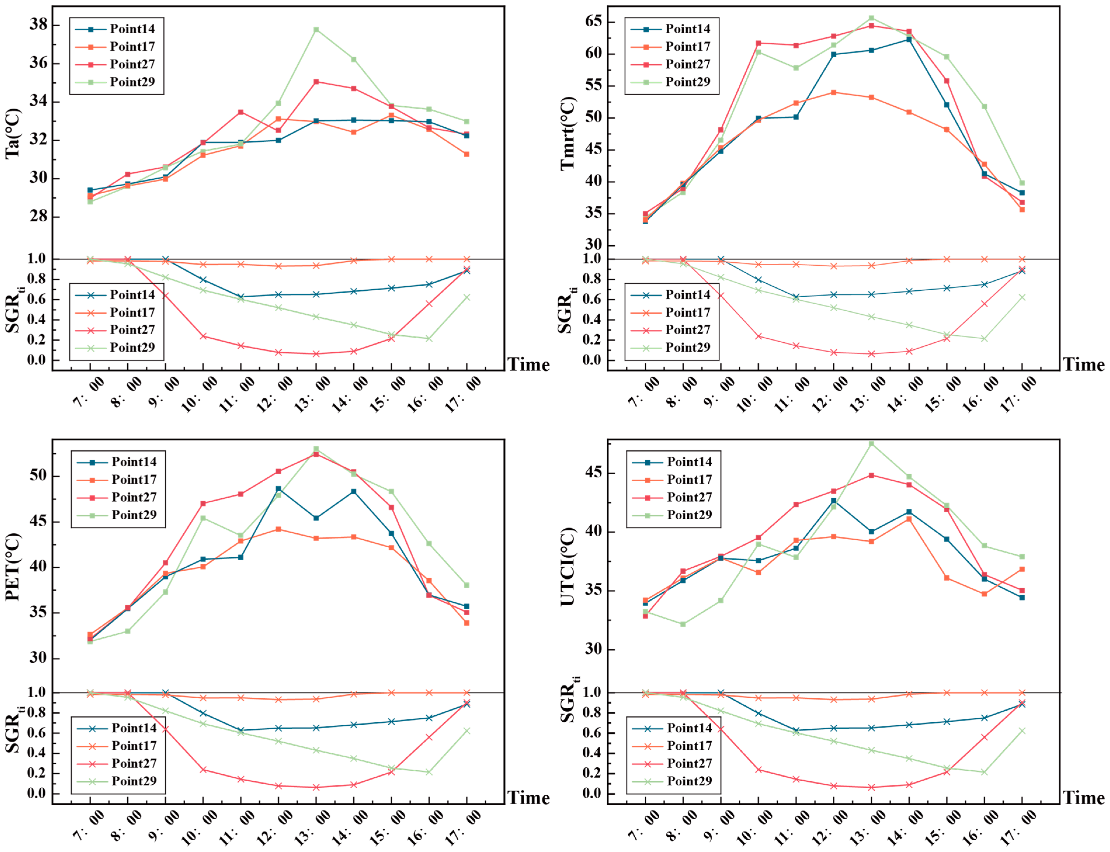
The selected points encompass diverse morphological configurations: point 17 exhibits the highest SGR and lowest SVF among all sites, point 27 has the lowest SGR, point 29 has the highest SVF, and point 14 shows medium values for both SGR and SVF. As shown in Figure 13, SGR at these four points first decreased and then increased, with higher values in the morning and late afternoon and minima around 13:00, going down and up dramatically in the morning and afternoon. In the midday, from 11:00 (a.m.) to 14:00 (p.m.) the SGRti values maintain a smooth pace, except for point 29. A gazebo in the eastern part of the site provides shadow for this point in the morning. Ta showed diurnal fluctuations of up to 10.52 °C at point 29, with the most intense fluctuations concentrated between 12:00 and 15:00. By contrast, the point with the lowest SGR (point 27) exhibited considerably smaller diurnal temperature fluctuations, though still greater than those observed at points 14 and 17, which had higher SGR and lower SVF.
Figure 13.
Trend of all-day temperature and thermal comfort for points 14, 17, 27 and 29.
Tmrt demonstrated greater sensitivity to shadow conditions, with substantial differences among measurement points. At point 17, Tmrt remained below 45 °C throughout the day, with minimal fluctuation, whereas at point 27, Tmrt surged sharply above 60 °C during the midday, exhibiting fluctuations exceeding 20 °C. Points 14 and 29 showed Tmrt variations that fell between these two extremes. These pronounced Tmrt fluctuations directly reflect the instantaneous effects of solar radiation obstruction.
Point 17 exhibited the smallest diurnal variations in both PET and UTCI, maintaining a relatively comfortable range throughout the day. In contrast, point 27 displayed pronounced midday peaks, with PET and UTCI surpassing 42 °C and 39 °C, respectively, indicating severe heat stress. Points 14 and 29 again showed intermediate patterns between these extremes. Taken together, these observations indicate that locations with higher SGR not only show greater thermal stability but also maintain relatively lower levels of thermal stress throughout the day. This finding has important implications for summer heat mitigation in hot and humid areas.
The influence of SGR on the thermal environment and thermal comfort exhibits a diurnal variation. In the morning hours, a higher SGR effectively slows the rising rates of air temperature and mean radiant temperature, thereby delaying the accumulation of thermal load. Around midday, the higher the SGR, the lower the peak temperature at a given measurement point, and the differences in both thermal environment and thermal comfort metrics among points reach their daily maximum. In the afternoon, the effect of SGR on the decreasing rates of thermal environment and thermal comfort metrics becomes less pronounced.
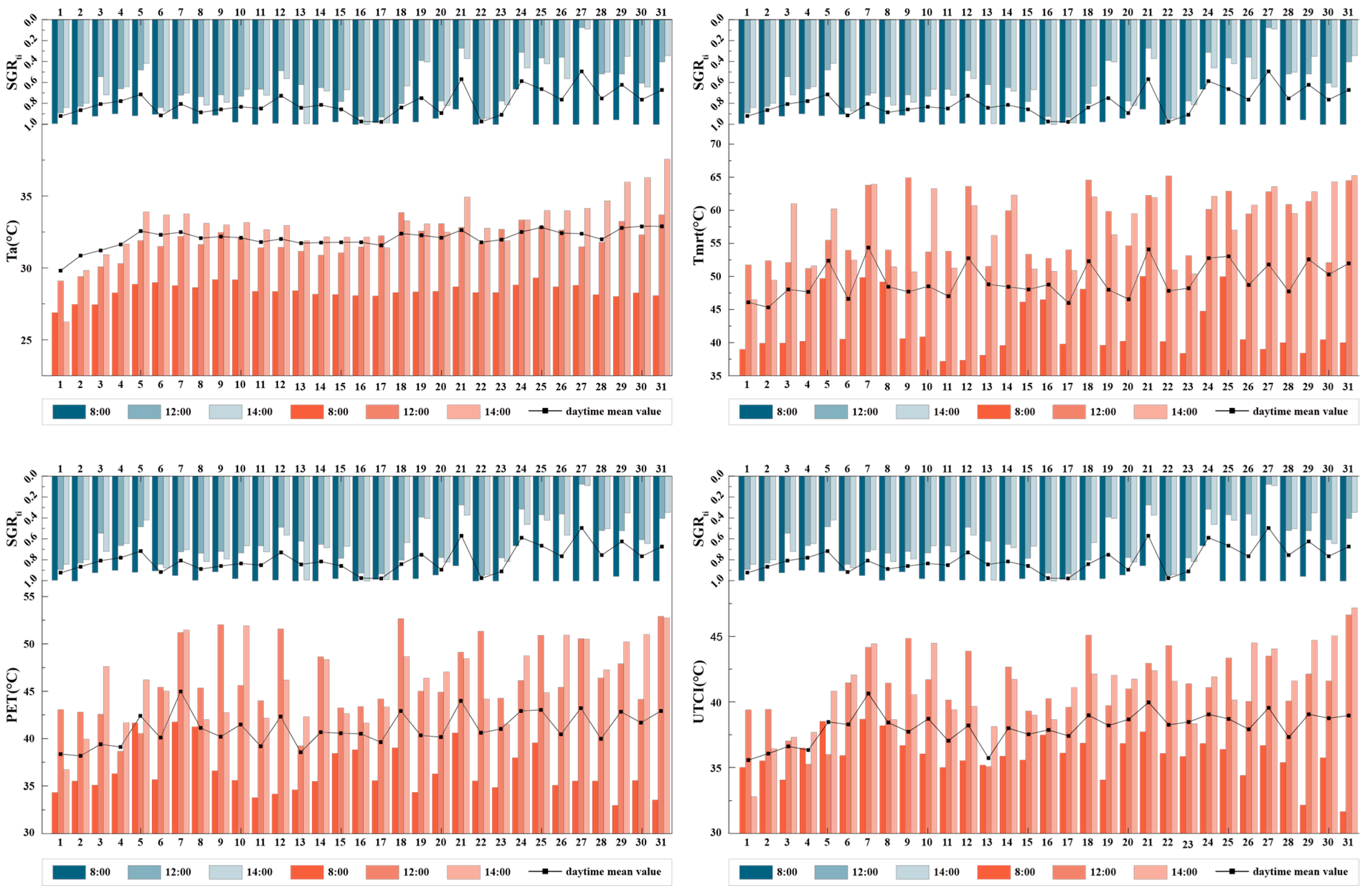
Three representative time points were selected for analysis: 8:00 (high SGR baseline), 12:00 (solar noon), and 14:00 (peak thermal stress). Divergent shading configurations across the sites yielded significant microclimatic heterogeneity. While inter-site temperature gradients were negligible during the early morning (8:00), they intensified substantially by midday (12:00) and reached their maximum during the afternoon (14:00). At 14:00, the spatial polarization of Ta peaked, with the fully exposed point 31 reaching 37.56 °C, while the continuously shaded point 1 remained at 28.13 °C—a striking 9.43 °C gap. During the midday to afternoon period (12:00–17:00), Tmrt exhibited pronounced fluctuations across points, underscoring an inhomogeneous radiative field. Likewise, thermal comfort indices displayed high spatial variability, reinforcing the intrinsic link between instantaneous shadow coverage, radiative flux, and human thermal comfort (Figure 14).
Figure 14.
Temperature and thermal comfort variation for all 31 points, with all-day average and at 8:00, 12:00 and 14:00.
4. Discussion
4.1. Practicality and Operational Feasibility of the PPM Framework
The proposed PPM framework for shadow measurement achieves a balance between measurement precision and operational practicality. Validation against UAV-derived shadow ratios yielded a MRE of 1.69% and a RMSE of 0.030, indicating a high degree of agreement between the two datasets.
Beyond accuracy, unlike model-based calculation methods, the approach does not rely on geometric simplifications, thereby avoiding systematic errors that may arise in the complex urban environment. Operating at the pedestrian scale, it can be used to represent complex shadows, including the irregular boundaries of canopies and those attenuated by foliage gaps or cast by architectural elements such as balustrades and awnings. The image processing and calculation in each grid element treats lights filtering through the gaps between leaves as sunlit areas and calculates the precise value, which makes it possible to identify the light transmittance specifically in each site. The workflow requires minimal hardware, which facilitates both in situ deployment and cross-site scalability. Compared to pixel-based methods [26], the PPM framework provides a wider field of view.
From a hardware perspective, in contrast to conventional fisheye lenses, the panoramic camera is more widely available and produces images with more predictable geometric properties. Recent studies have demonstrated that panoramic imagery can be reliably converted into sky-view fisheye images for batch calculation of the SVF [45,46,47,48]. In field applications, the panoramic system only requires a fixed mounting height, without the need for precise horizontal orientation adjustments. This feature reduces operational complexity, particularly for large-scale measurement campaigns. Moreover, fisheye images derived from panoramic photographs retain a stable imaging center aligned with the vertical normal, which ensures consistent perspectives across batch images and helps reduce measurement error. Additionally, a single panoramic image can be used to generate both sky-view and ground-view fisheye projections, allowing for concurrent calculation of SVF and SGR, further improving data collection efficiency.
Methodologically, the PPM framework quantifies shadow area directly in the original, distorted fisheye images, rather than rectifying the images into orthophotos. This strategy was adopted for practical reasons. First, without three-dimensional control points or camera calibration parameters, a single fisheye image is difficult to correct into orthophotos. Even after correction, the resulting image still requires secondary quantification through additional calibration, which increases procedural complexity [49]. Second, extracting distorted shadow contours and then correcting them point by point to real-world spatial positions through coordinate transformation is not only procedurally cumbersome, but may also introduce cumulative error.
Instead, the PPM method constructs a nonlinear distortion grid directly on the original image, based on the equidistant projection model. Through grid calibration using on-site reference objects, it establishes a mapping between pixel area in the image and actual ground area. This approach has two characteristics. First, it does not require elaborate calibration or image rectification, which reduces procedural complexity. Second, the small residual distortions remaining after grid calibration are randomly distributed across cells. Consequently, their effects on shadow area estimation tend to offset one another during summation, which helps limit the accumulation of systemic error.
To ensure the application of the PPM framework in other outdoor environments such as university campuses, we provide the following caveats:
- Camera height must be fixed, and grid calibration should be based on on-site references (e.g., pavement tiles);
- Binarization currently requires manual assistance, which may introduce minor operator variability;
- The 10 m radius was limited by the camera’s field of view; a larger radius would cause excessive compression at fisheye image edges and reduce accuracy.
Following these steps, the method can be reproduced at other sites.
4.2. Comparative Performance of SGR and SVF in an Outdoor Thermal Environment Evaluation
This study introduces a shadow ratio indicator SGR to quantify combined shadow coverage within complex outdoor environments. By integrating spatiotemporal dimensions, SGR characterizes the dynamic shadow morphologies formed collectively by buildings, trees, and other shading elements.
The strong negative correlation between SGR and SVF validates the proposed indicator. A lower SVF value indicates increased sky obstruction, typically translating into higher shadow coverage. This aligns with our previous study by Xu et al., which reported a significant negative correlation between BSGR and SVF—an association that is contingent upon solar geometry [15]. One superior aspect of SGR is that it simultaneously describes the obstruction from surroundings, solar radiation and solar azimuth for a site, and SVF merely focused on the first one. Namely, SVF is an isotropic indicator, for which the correlation with solar radiation strengthens within specific angular ranges [8]. For example, a northern obstruction reduces SVF, yet casts no shadow when the sun is in the south, thus providing no actual shading. This represents a fundamental distinction: while SVF serves as an indirect proxy for shading based on sky visibility, SGR provides a direct, dynamic, and geometry-based quantification of actual shadow conditions. Compared with BSGR, which also simultaneously captures the geographical and temporal characteristics of the site, SGR has filled in the simplified details by taking all the shading objects. This horizontal expansion makes the indicator measurable and verifiable, and also more accurately describes the shadow.
SGR correlates significantly with thermal environment and comfort parameters, as governed by each variable’s sensitivity to solar radiation. Solar radiation has significant impacts with respect to thermal environment and thermal comfort indicators, except for Va, and these impacts manifested in the correlations between SGR and the indicators [50,51]. Tmrt, most sensitive to shortwave radiation, shows the highest correlation, with SGR (R2 = 0.583), as it is reduced by intercepting solar radiation [52]. Similarly, UTCI, which incorporates radiation’s impact, also exhibits stronger linear correlations with SGR than with SVF. Meanwhile, instantaneous shadow coverage drives spatial thermal differentiation: shading variance causes air temperature gaps of nearly 10 °C, with Tmrt effects peaking in the afternoon. Thus, in hot and humid areas, solar radiation dictates outdoor thermal comfort, and shadow coverage is the most direct physical intervention for mitigating radiant heat [22].
SVF, in contrast, exhibits a stronger correlation with RH than SGR. A study in hot and humid areas showed that SVF has a negative correlation with Va, and points with high SVF have low ventilation [53]. In highly enclosed high-VF environments with extensive obstructions as well as lower wind velocity, water vapor tends to persist longer, elevating RH levels. These obstructions not only restrict horizontal air movement but also reduce surface evaporation—effects that are orientation-independent, thus explaining the stronger correlation between SVF and RH [54].
Time-series analysis further shows that shadow indicators effectively characterize daytime thermal stability, with SVF exhibiting slightly stronger correlations with fluctuations than SGR. This suggests that SVF is a superior indicator for assessing the stability of both microclimatic conditions and thermal comfort. Time-series analysis reveals that low SVF (often associated with high SGR) induces gradual diurnal comfort fluctuations, with heat stress remaining consistently low throughout the day.
4.3. Limitations
While this study establishes a robust framework for shadow quantification and thermal analysis, several limitations remain:
1. A series of constraints encountered during the experimental process will to some extent affect the accuracy of the data in the result. Site constraints at point A limited the ideal validation of PPM accuracy. Firstly, a tree canopy (≈3 m diameter) at the northeast corner of the measurement circle partially obstructed the UAV’s orthogonal image, causing SGRUAV underestimation, mainly between 11:20 and 13:10 and after 14:40. Secondly, SGR is sensitive to the calculation radius; our previous study identified an optimum of 15–20 m [15], but the camera’s limited field of view and site conditions forced us to fix the radius at 10 m. This compromise may reduce SGR’s performance. Moreover, we did not systematically examine SGR’s correlations with thermal indicators under varying radii. Thirdly, Tmrt was estimated using the RayMan model because conventional methods requiring long stabilization times or specialized equipment were incompatible with our mobile transect design, introducing unavoidable uncertainties. Future work should prioritize unobstructed sites, use a larger field of view to match the optimal radius, test multiple radii, and incorporate precision radiometers to balance multi-site surveys with time constraints to refine empirical datasets.
2. PPM requires further refinement due to three primary bottlenecks. First, binarization lacks precision and automation, relying on manual tuning and ignoring irregular vegetation footprints (e.g., trunks). Although these footprints cause negligible errors, processing time increases significantly. Also, the lighting condition has an impact on the determination of shadow boundaries, a factor which would cause minor errors. Second, unlike building shadows, tree crowns allow partial solar penetration, meaning tree-shade intensity lies between 0 and 1, but binarization treats shadows as binary, ignoring leaf transmissivity. Third, the issue of computational time in Grasshopper scales with shadow contour complexity; irregular contours can quadruple per-cell time. Processing >2500 cells per image (multiple images per point) creates a heavy cumulative burden. Automated shadow segmentation, higher-resolution images with advanced techniques and grid pre-selection should be adopted in future work to refine image processing, differentiate shade translucency and improve computational efficiency.
3. Some questions remain to be further discussed at the current stage of the study. The field measurements in this study were conducted only on a sunny summer day; the behavior of SGR in winter or other seasons remains unexplored. Future research should extend the measurements to different seasons to fully assess the impact of SGR on thermal environment and comfort across the annual cycle. Moreover, the differences in shading characteristics among different shading objects remain unclear. Among the 31 measurement points, only three were solely shaded by buildings, while the rest were either shaded by trees alone or by both buildings and trees. This indicates that the current sample size is insufficient for reliably assessing the differences between building and tree shadows. Finally, the conclusions in this study are intended only for low-density, green-rich areas in hot and humid regions. How the proposed indicator performs in other regions with different morphologies and climates remains to be further studied.
5. Conclusions
This study defined the shadow geographical ratio (SGR) to quantify combined building–tree shadow coverage in complex environments and proposed a panoramic photo-based method (PPM) framework. Based on measurements recorded at Xiamen University, we validated the reliability of the SGR and PPM frameworks, and, further, compared how SGR and SVF differentially relate to the thermal environment.
The main conclusions are as follows:
1. The PPM framework achieved high accuracy. Validated against UAV-derived benchmarks, it yielded a MRE of 1.69% and a RMSE of 0.030, confirming its capability for field-based acquisition of combined building–tree shadow ratio data.
2. The PPM framework demonstrated technical applicability to complex environments. Focused on the pedestrian scale, it effectively captured intricate shadows cast by built structures and vegetation. The measurement required only a panoramic camera with minimal hardware demands, and exhibited robust error control.
3. SGR showed a strong negative correlation with SVF. Except for RH, SGR exhibited higher sensitivity to most thermal environment and thermal comfort indicators, including Ta, Tmrt, UTCI, and PET.
4. SVF showed a slightly stronger association with thermal environment stability than did SGR. Sites with lower SVF and higher SGR experienced reduced diurnal fluctuations in temperature and thermal comfort, maintaining relatively stable thermal conditions throughout the daytime.
This study provides a tool for quantifying combined building–tree shadows. Key contributions include extending shadow quantification from single to combined types and shifting from macro-blocks to the pedestrian scale, filling a methodological gap in complex environments. The study also validates SGR as a complement to SVF for assessing shadow-driven thermal regulation in hot and humid areas. Future work will refine the experimental setup—including site selection and measurement instrumentation—to improve PPM accuracy and robustness; systematically examine the effect of calculation radius on SGR; and improve computational efficiency via automated shadow segmentation and grid pre-selection.
Author Contributions
L.J.: Conceptualization, Methodology, Resources, Writing—original draft, Formal analysis, Funding acquisition. L.C.: Writing—original draft, Investigation, Visualization, Validation, Data curation, Formal analysis. X.H.: Methodology, Writing—review and editing, Supervision, Resources. Y.L.: Investigation, Resources, Software. All authors have read and agreed to the published version of the manuscript.
Funding
This research was funded by National Natural Science Foundation of China (grant number: 52108033) and the Fundamental Research Funds for the Central Universities (grant number: 20720220116). The APC was funded by National Natural Science Foundation of China (grant number: 52108033).
Data Availability Statement
All data involved in this study are included in the article. Further inquiries can be directed to the corresponding author.
Acknowledgments
During the preparation of this work, the authors used ChatGPT (version 5.2, OpenAI, San Francisco, CA, USA) for language editing and improvement of clarity. The authors have reviewed and edited the output and take full responsibility for the content.
Conflicts of Interest
The authors declare that they have no known competing financial interests or personal relationships that could have appeared to influence the work reported in this paper.
Nomenclature
| Ta | Air temperature |
| Va | Air velocity |
| BSGR | Building shadow geographical ratio |
| MRE | Mean relative error |
| Tmrt | Mean radiant temperature |
| PET | Physiologically equivalent temperature |
| PPM | Panoramic photo-based measurement |
| RH | Relative humidity |
| RMSE | Root mean square error |
| SGR | Shadow geographical ratio |
| SVF | Sky view factor |
| SD | Standard deviation |
| UAV | Unmanned aerial vehicle |
| UTCI | Universal thermal climate index |
Appendix A
Figure A1.
Correlation between RBSGR and Ta, Tg, Tmrt, UTCI, and PET [15]. For Ta, R210m = 0.858, R220m = 0.922, r10m = −0.599, r20m = −0.650; for Tmrt, R210m = 0.945, R220m = 0.993, r10m = −0.667, r20m = −0.702; for UTCI, R210m = 0.753, R215m = 0.771, r10m = −0.503, r15m = −0.521; for PET, R210m = 0.717, R217.5m = 0.741, r10m = −0.467, r20m = −0.491.
Appendix B
Table A1.
Detailed image-processing workflow.
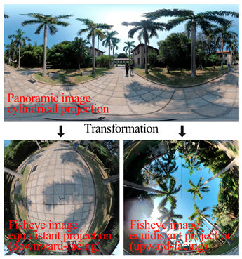
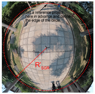
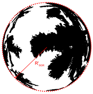

Table A2.
Detailed grid establishment workflow.
Appendix C
Table A3.
Results of successfully fitted models.
References
- Li, Y.G.; Huang, N.X.; He, J. Analytical evaluation of thermal comfort in the pedestrian environment using pedestrian shade space distribution. Urban Clim. 2023, 51, 101665. [Google Scholar] [CrossRef] [Scilit]
- Gai, Z.; Yin, H.; Kong, F.; Su, J.; Shen, Z.; Sun, H.; Yang, S.; Liu, H.; Middel, A. How does shade infrastructure affect outdoor thermal comfort during hot, humid summers? Evidence from Nanjing, China. Build. Environ. 2025, 267, 112320. [Google Scholar] [CrossRef] [Scilit]
- Liu, J.Y.; Tang, H.F.; Zheng, B.H. Thermal Environments of Residential Areas: Sunlight and Building Shadow in a Chinese City with Hot and Humid Summers. Buildings 2024, 14, 28. [Google Scholar] [CrossRef] [Scilit]
- Liu, Z.M.; Li, J.; Xi, T.Y. A Review of Thermal Comfort Evaluation and Improvement in Urban Outdoor Spaces. Buildings 2023, 13, 32. [Google Scholar] [CrossRef] [Scilit]
- Sakhri, H.; Bada, Y.; Emmanuel, R. Study on correlation between shadow patterns and human behaviour in hot, arid cities: A case study of Biskra, Algeria. Int. J. Biometeorol. 2022, 66, 2517–2528. [Google Scholar] [CrossRef] [Scilit] [PubMed]
- Li, Y.Q.; Liu, X.; Cheshmehzangi, A.; Zahed, L.M.; He, B.J. Multidimensional factors affecting tree-induced cooling benefits: A comprehensive review. Build. Environ. 2025, 282, 48. [Google Scholar] [CrossRef] [Scilit]
- Du, J.; Liu, L.; Chen, X.; Liu, J. Field Assessment of Neighboring Building and Tree Shading Effects on the 3D Radiant Environment and Human Thermal Comfort in Summer within Urban Settlements in Northeast China. Adv. Meteorol. 2020, 2020, 1–19. [Google Scholar] [CrossRef] [Scilit]
- Li, W.; Zhou, Z.; Zhang, S.; Feng, J. Study on Relationship between Shading and Outdoor Air Temperature Based on the Comparison of Two High-Rise Residential Estates with Field Measurements. Buildings 2022, 12, 1813. [Google Scholar] [CrossRef] [Scilit]
- Han, Y.; Jo, Y.; Kim, E.J. Influence of landscape interventions on thermal comfort under time-varying building shadow; new Gwanghwamun square case, Seoul, South Korea. Heliyon 2023, 9, e19436. [Google Scholar] [CrossRef] [Scilit] [PubMed]
- Sun, T.; Chen, L.D.; Sun, R.H. Cooling effects in urban communities: Parsing green spaces and building shadows. Urban For. Urban Green. 2024, 94, 7. [Google Scholar] [CrossRef] [Scilit]
- Yang, J.; Zhao, Y.; Guo, T.; Luo, X.; Ji, K.; Zhou, M.; Wan, F. The impact of tree species and planting location on outdoor thermal comfort of a semi-outdoor space. Int. J. Biometeorol. 2023, 67, 1689–1701. [Google Scholar] [CrossRef] [Scilit]
- Kim, J.Y.; Park, C.Y.; Hyun, J.H.; Kim, S.H.; Yun, S.H.; Lee, D.K. Landscape Design for Improved Thermal Environment: An Optimized Tree Arrangement Design for Climate-Responsive Outdoor Spaces in Residential Buildings Complexes. Sustain. Cities Soc. 2023, 97, 104762. [Google Scholar] [CrossRef] [Scilit]
- Kim, J.Y.; Park, C.Y.; Lee, D.K.; Yun, S.H.; Hyun, J.H.; Kim, E.S. The cooling effect of trees in high-rise building complexes in relation to spatial distance from buildings. Sustain. Cities Soc. 2024, 114, 105737. [Google Scholar] [CrossRef] [Scilit]
- JGJ 286-2013; Thermal Environment Design Standard for Urban Residential Areas. Ministry of Housing and Urban-Rural Development of China: Beijing, China, 2013.
- Xu, Y.; Jia, L.; Hong, X. An optimized index for describing building shadows to assess the local thermal environment of residential areas in summer. Build. Environ. 2025, 270, 112573. [Google Scholar] [CrossRef] [Scilit]
- Song, J.; Liu, Y.; Liu, B.; Ren, J. Seasonal effects of residential morphology on insolation shadow ratio in Xi’an: A machine learning approach. Build. Environ. 2025, 282, 16. [Google Scholar] [CrossRef] [Scilit]
- Aleksandrowicz, O.; Zur, S.; Lebendiger, Y.; Lerman, Y. Shade maps for prioritizing municipal microclimatic action in hot climates: Learning from Tel Aviv-Yafo. Sustain. Cities Soc. 2020, 53, 19. [Google Scholar] [CrossRef] [Scilit]
- Oke, T.R. Boundary Layer Climates; Routledge: London, UK, 1978. [Google Scholar]
- Jamei, E.; Rajagopalan, P.; Seyedmahmoudian, M.; Jamei, Y. Review on the impact of urban geometry and pedestrian level greening on outdoor thermal comfort. Renew. Sust. Energ. Rev. 2016, 54, 1002–1017. [Google Scholar] [CrossRef] [Scilit]
- Svensson, M.K. Sky view factor analysis—Implications for urban air temperature differences. Meteorol. Appl. 2004, 11, 201–211. [Google Scholar] [CrossRef] [Scilit]
- Yan, H.; Fan, S.X.; Guo, C.X.; Wu, F.; Zhang, N.; Dong, L. Assessing the effects of landscape design parameters on intra-urban air temperature variability: The case of Beijing, China. Build. Environ. 2014, 76, 44–53. [Google Scholar] [CrossRef] [Scilit]
- Kong, F.H.; Chen, J.Y.; Middel, A.; Yin, H.W.; Li, M.C.; Sun, T.; Zhang, N.; Huang, J.; Liu, H.Q.; Zhou, K.J.; et al. Impact of 3-D urban landscape patterns on the outdoor thermal environment: A modelling study with SOLWEIG. Comput. Environ. Urban Syst. 2022, 94, 13. [Google Scholar] [CrossRef] [Scilit]
- Ali-Toudert, F.; Mayer, H. Numerical study on the effects of aspect ratio and orientation of an urban street canyon on outdoor thermal comfort in hot and dry climate. Build. Environ. 2006, 41, 94–108. [Google Scholar] [CrossRef] [Scilit]
- Peeters, A.; Shashua-Bar, L.; Meir, S.; Shmulevich, R.R.; Caspi, Y.; Weyl, M.; Motzafi-Haller, W.; Angel, N. A decision support tool for calculating effective shading in urban streets. Urban Clim. 2020, 34, 12. [Google Scholar] [CrossRef] [Scilit]
- Zhou, X.; Shen, X.H.; Liu, Z.R.; Sun, H.S.; An, J.J.; Yan, D. A novel shadow calculation approach based on multithreaded parallel computing. Energy Build. 2024, 312, 15. [Google Scholar] [CrossRef] [Scilit]
- Rocha, A.P.D.; Reynoso-Meza, G.; Oliveira, R.; Mendes, N. A pixel counting based method for designing shading devices in buildings considering energy efficiency, daylight use and fading protection. Appl. Energy 2020, 262, 11. [Google Scholar] [CrossRef] [Scilit]
- Liu, Z.R.; Zhou, X.; Shen, X.H.; Sun, H.S.; Yan, D. A novel acceleration approach to shadow calculation based on sunlight channel for urban building energy modeling. Energy Build. 2024, 315, 14. [Google Scholar] [CrossRef] [Scilit]
- Yezioro, A.; Shaviv, E. Shading—A design tool for analyzing mutual shading between buildings. Sol. Energy 1994, 52, 27–37. [Google Scholar] [CrossRef] [Scilit]
- Rocha, A.P.D.; Oliveira, R.; Mendes, N. Experimental validation and comparison of direct solar shading calculations within building energy simulation tools: Polygon clipping and pixel counting techniques. Sol. Energy 2017, 158, 462–473. [Google Scholar] [CrossRef] [Scilit]
- Zaki, S.A.; Syahidah, S.W.; Shahidan, M.F.; Ahmad, M.I.; Yakub, F.; Hassan, M.Z.; Daud, M.Y.M. Assessment of Outdoor Air Temperature with Different Shaded Area within an Urban University Campus in Hot-Humid Climate. Sustainability 2020, 12, 24. [Google Scholar] [CrossRef] [Scilit]
- Azcarate, I.; Acero, J.A.; Garmendia, L.; Rojí, E. Tree layout methodology for shading pedestrian zones: Thermal comfort study in Bilbao (Northern Iberian Peninsula). Sustain. Cities Soc. 2021, 72, 102996. [Google Scholar] [CrossRef] [Scilit]
- Nazarian, N.; Fan, J.P.; Sin, T.; Norford, L.; Kleissl, J. Predicting outdoor thermal comfort in urban environments: A 3D numerical model for standard effective temperature. Urban Clim. 2017, 20, 251–267. [Google Scholar] [CrossRef] [Scilit]
- Chen, Q.; Liu, R.; Cheng, Q.H.; Chen, Y.H.; Cao, S.S.; Du, M.Y.; Li, K.N. Evaluating the impact of sky view factor and building shadow ratio on air temperature in different residential and commercial building scenarios: A case study of Beijing, China. Urban Clim. 2023, 49, 20. [Google Scholar] [CrossRef] [Scilit]
- Wang, Q.Q.; Peng, L.L.H.; Jiang, W.; Yin, S.; Feng, N.Y.; Yao, L.Y. Urban form affects the cool island effect of urban greenery via building shadows. Build. Environ. 2024, 254, 111398. [Google Scholar] [CrossRef] [Scilit]
- Yu, B.L.; Liu, H.X.; Wu, J.P.; Lin, W.M. Investigating impacts of urban morphology on spatio-temporal variations of solar radiation with airborne LIDAR data and a solar flux model: A case study of downtown Houston. Int. J. Remote Sens. 2009, 30, 4359–4385. [Google Scholar] [CrossRef] [Scilit]
- Lindberg, F.; Grimmond, C.S.B. Nature of vegetation and building morphology characteristics across a city: Influence on shadow patterns and mean radiant temperatures in London. Urban Ecosyst. 2011, 14, 617–634. [Google Scholar] [CrossRef] [Scilit]
- Suziedelyte Visockiene, J.; Puziene, R.; Stanionis, A.; Tumeliene, E. Unmanned Aerial Vehicles for Photogrammetry: Analysis of Orthophoto Images over the Territory of Lithuania. Int. J. Aerosp. Eng. 2016, 2016, 3. [Google Scholar] [CrossRef] [Scilit]
- Honjo, T.; Lin, T.P.; Seo, Y. Sky view factor measurement by using a spherical camera. J. Agric. Meteorol. 2019, 75, 59–66. [Google Scholar] [CrossRef] [Scilit]
- Höppe, P. The physiological equivalent temperature -: A universal index for the biometeorological assessment of the thermal environment. Int. J. Biometeorol. 1999, 43, 71–75. [Google Scholar] [CrossRef] [Scilit]
- Bröde, P.; Fiala, D.; Blazejczyk, K.; Holmér, I.; Jendritzky, G.; Kampmann, B.; Tinz, B.; Havenith, G. Deriving the operational procedure for the Universal Thermal Climate Index (UTCI). Int. J. Biometeorol. 2012, 56, 481–494. [Google Scholar] [CrossRef] [Scilit]
- Middel, A.; Huff, M.; Krayenhoff, E.S.; Udupa, A.; Schneider, F.A. PanoMRT: Panoramic infrared thermography to model human thermal exposure and comfort. Sci. Total Environ. 2023, 859, 13. [Google Scholar] [CrossRef] [Scilit]
- Matzarakis, A.; Rutz, F.; Mayer, H. Modelling radiation fluxes in simple and complex environments—Application of the RayMan model. Int. J. Biometeorol. 2007, 51, 323–334. [Google Scholar] [CrossRef] [Scilit]
- Yan, H.; Wu, F.; Nan, X.E.; Han, Q.; Shao, F.; Bao, Z.Y. Influence of view factors on intra-urban air temperature and thermal comfort variability in a temperate city. Sci. Total Environ. 2022, 841, 11. [Google Scholar] [CrossRef] [Scilit]
- Virtanen, P.; Gommers, R.; Oliphant, T.E.; Haberland, M.; Reddy, T.; Cournapeau, D.; Burovski, E.; Peterson, P.; Weckesser, W.; Bright, J.; et al. SciPy 1.0: Fundamental algorithms for scientific computing in Python. Nat. Methods 2020, 17, 261–272. [Google Scholar] [CrossRef] [Scilit]
- Du, K.; Ning, J.; Yan, L. How long is the sun duration in a street canyon?—Analysis of the view factors of street canyons. Build. Environ. 2020, 172, 106680. [Google Scholar] [CrossRef] [Scilit]
- Gong, F.-Y.; Zeng, Z.-C.; Zhang, F.; Li, X.; Ng, E.; Norford, L.K. Mapping sky, tree, and building view factors of street canyons in a high-density urban environment. Build. Environ. 2018, 134, 155–167. [Google Scholar] [CrossRef] [Scilit]
- Tian, L.; Hao, T.; He, X.; Chan, I.; Niu, J.; Chan, P.W.; Ng, W.Y.; Huang, J. Examining the non-linear relationship between urban form and air temperature at street level: A case of Hong Kong. Build. Environ. 2024, 264, 111884. [Google Scholar] [CrossRef] [Scilit]
- Yıldız, N.D.; Erdem, F.; Acet, S.B.; Avdan, U. Analyzing the effect of view factors on surface heat flux, surface temperature, and vegetation cover. Environ. Sci. Pollut. Res. 2023, 30, 43843–43859. [Google Scholar] [CrossRef] [Scilit]
- Zhou, G.Q.; Li, H.X.; Song, R.H.; Wang, Q.Y.; Xu, J.S.; Song, B. Orthorectification of Fisheye Image under Equidistant Projection Model. Remote Sens. 2022, 14, 4175. [Google Scholar] [CrossRef] [Scilit]
- Lyu, T.; Buccolieri, R.; Gao, Z. A Numerical Study on the Correlation between Sky View Factor and Summer Microclimate of Local Climate Zones. Atmosphere 2019, 10, 438. [Google Scholar] [CrossRef] [Scilit]
- Yola, L.; Siong, H.C. Solar Radiation and Urban Wind Effect on Urban Canyon in Hot, Humid Regions. In Proceedings of the 7th Asia Pacific International Conference on Environment-Behaviour Studies, Scotland, UK, 27 July–30 September 2016; pp. 220–229. [Google Scholar]
- Park, C.Y.; Lee, D.K.; Krayenhoff, E.S.; Heo, H.K.; Ahn, S.; Asawa, T.; Murakami, A.; Kim, H.G. A multilayer mean radiant temperature model for pedestrians in a street canyon with trees. Build. Environ. 2018, 141, 298–309. [Google Scholar] [CrossRef] [Scilit]
- Leder, S.M.; Bezerra, M.d.L.F.D.; Souza, E.L.d. Exploring urban form and microclimatic variables in a hot-humid city. PARC Pesqui. Arquitetura Construção 2025, 16, e025020. [Google Scholar] [CrossRef] [Scilit]
- Kalanda, B.D.; Oke, T.R.; Spittlehouse, D.L. Suburban Energy Balance Estimates for Vancouver, B.C., Using the Bowen Ratio-Energy Balance Approach. J. Appl. Meteorol. Climatol. 1980, 19, 791–802. [Google Scholar] [CrossRef] [Scilit]






Disclaimer/Publisher’s Note: The statements, opinions and data contained in all publications are solely those of the individual author(s) and contributor(s) and not of MDPI and/or the editor(s). MDPI and/or the editor(s) disclaim responsibility for any injury to people or property resulting from any ideas, methods, instructions or products referred to in the content. |
© 2026 by the authors. Licensee MDPI, Basel, Switzerland. This article is an open access article distributed under the terms and conditions of the Creative Commons Attribution (CC BY) license.