


Abstract
To ensure a reliable electrical isolation point in power systems, the seismic performance assessment of disconnect switches is of critical importance for maintaining operational continuity under earthquake excitations. In this study, a hybrid method combining a convolutional neural network (CNN) and a long short-term memory (LSTM) network is proposed for the seismic intelligent classification and response prediction of disconnect switches. Unlike conventional approaches that rely on finite element simulations or shake table tests with high computational costs, the proposed method learns directly from raw ground motion records. The CNN component is designed to capture local frequency characteristics of input ground motions, enabling automatic classification into low-, medium-, or high-frequency categories. Subsequently, category-specific LSTM models are established to map the ground motion time series to multi-dimensional performance indicators of the disconnect switch. These indicators include top absolute accelerations, bottom shear forces, and relative deformations of porcelain posts. A training set comprising 102 ground motion records is constructed based on numerical simulations of a validated simplified model, while another testing set comparing 21 ground motion records are employed to validate the performance of predicted models. Training and validation results demonstrate that the CNN achieves a great classification accuracy. The LSTM predictions show good agreement with the computed time-history responses, with errors of root-mean-square responses generally within 10%. The proposed method provides a rapid, data-driven alternative to traditional seismic analysis, significantly reducing computational time while preserving prediction fidelity. It also enables the parallel prediction of multiple coupled performance indicators, which is not readily achievable by existing single-output surrogate models.
1. Introduction
Modern society depends heavily on the continuous operation of electric power systems. Among the various components of a power grid, substation equipment—particularly disconnect switches—plays a vital role in ensuring safe maintenance and fault isolation. However, these slender, porcelain-based structures are known to be highly vulnerable to earthquake-induced damage. Traditional seismic performance assessment relies on finite element simulations or shake-table tests, which are computationally expensive and time-consuming. There is therefore a growing need for rapid, accurate, and data-driven surrogate models that can predict the seismic response of such equipment in real time.
Power infrastructure constitutes a critical foundation for ensuring national security and socioeconomic development. A power grid generally consists of power plants [1,2], transmission lines [3,4] spanning urban and rural areas, substations, converter stations, and urban power distribution systems. Among these components, the operational environment of substation equipment is particularly harsh, and various natural hazards—such as earthquakes [5], landslides [6], and debris flows [7]—severely affect its performance. Among these natural disasters, earthquakes [8,9,10] are the most destructive and may cause huge economic losses and casualties, which deserve special attention [11,12,13]. Notable examples include the Kahramanmaraş earthquakes in 2023 [14,15,16] and the Balıkesir earthquake in 2025 [17]. Substations are especially susceptible to seismic events because most high-voltage equipment installed therein is slender and features dense, heavy masses at the top [18]. Moreover, the insulators used in most such equipment are made of porcelain, a material characterized by high electrical resistance but extreme brittleness. Seismic damage experiences worldwide have demonstrated that other types of infrastructure are heavily reliant on power infrastructure. For example, in the 1994 Northridge earthquake, damage to substation components in the western United States and the Los Angeles area led to power outages [19]. It is thus evident that substation equipment at various voltage levels exhibits relatively weak seismic resistance, and improving their seismic performance has become a major direction in lifeline earthquake engineering research.
The disconnect switch is a critical safety device in power systems. Its core function is to achieve electrical isolation of circuits under no load conditions. This provides a reliable and visible electrical separation point for maintenance of power equipment, switching of operational modes, and isolation of faults. Its seismic performance directly affects the operational safety of substations and even regional power grids under seismic excitation. Once a disconnect switch is damaged by an earthquake, not only is the power supply of the affected line interrupted, but chain reactions may also be triggered. Such chain reactions include busbar voltage loss in the substation and maloperation of protective devices, thereby multiplying the extent of the outage. Therefore, accurate seismic performance assessment of disconnect switches is of decisive engineering significance for ensuring the functional continuity of power systems under seismic events. Paolacci et al. [20,21] conducted a seismic fragility study on disconnect switches and identified the porcelain columns and connectors as the most vulnerable components. Xie et al. [22] performed a shaking table test on a 220 kV disconnect switch, revealing that a fracture at the base of the porcelain column is a typical failure characteristic. Wen et al. [23] evaluated the comprehensive fragility of disconnect switches through a combination of experiments and finite element analysis. Whittaker et al. [24] developed a single-degree-of-freedom simplified model for porcelain columns in disconnect switches based on experimental findings. Moustafa and Mosalam [25] investigated the seismic response of a 550 kV disconnect switch experimentally and proposed full-structure and substructure concepts, illustrating the effectiveness and limitations of applying the substructure concept to disconnect switches. Bastami and Hajihasani [26] explored the dynamic response of disconnect switches under far-field and near-field ground motions. It can be observed that most existing studies have relied on shaking table tests or finite element simulations to investigate and analyze the seismic performance of disconnect switches, which entail high time and cost burdens. Although some studies have considered different ground motion types, namely far-field and near-field earthquakes, the predominant frequency components of ground motions and their potential influence on the seismic performance of disconnect switches have not yet been quantified in the analytical process.
To overcome the high computational cost and real-time limitations of finite element analysis, data-driven artificial intelligence [27,28,29] approaches offer a viable pathway for intelligent seismic classification and rapid prediction of time-series seismic responses of disconnect switches. Seismic classification is a time-series sequence classification task, for which commonly used models include hidden Markov models [30,31], recurrent neural networks [32,33], and their variants. However, hidden Markov models incorporate a strong Markov assumption—i.e., the current state depends only on the previous state—which makes it difficult to capture long-range dependencies, whereas ground motion records often exhibit contextual correlations spanning multiple time steps. Furthermore, hidden Markov models are inherently linear dynamic systems and struggle to fit complex nonlinear temporal evolution patterns. Recurrent neural networks can propagate historical information step by step through time and model dependencies of arbitrary sequence length. However, their recurrent structure requires sequential computation along time steps, which is difficult to parallelize. This results in training and inference speeds being limited by sequence length and leads to low efficiency on long sequences. Additionally, recurrent neural networks still suffer from information loss and gradient decay when handling long sequences. Although originally designed for image processing, the one-dimensional convolutional neural network (1D CNN) [34] exhibits unique advantages in time-series classification, effectively addressing the limitations of the aforementioned models. By sliding convolution kernels to compute inner products with local sequence windows, a 1D convolutional layer can automatically learn local waveform patterns in time-series signals. Multiple convolution kernels operate in parallel, generating multiple sets of local feature maps that constitute rich low-level feature representations. This mechanism of local connectivity and weight sharing endows the CNN with inherent robustness to translation (i.e., positional shifts in waveforms along the time axis), eliminating the need for complex temporal alignment as required by hidden Markov models. Moreover, forward propagation in a CNN relies primarily on convolution operations, which can be highly parallelized on GPUs via matrix multiplications, significantly improving computational efficiency. Therefore, in this study, a CNN is proposed for the seismic classification task to achieve time-series classification dominated by the predominant frequency characteristics of ground motions.
For the task of time-series response prediction of disconnect switches, commonly used models include the autoregressive integrated moving average model and recurrent neural networks [35]. The autoregressive integrated moving average model formulates the prediction task as a linear combination of historical values and a moving average of residual terms, which cannot accurately capture the nonlinear dynamic characteristics of actual seismic responses. Moreover, the autoregressive integrated moving average imposes stringent stationarity requirements on training data and exhibits low adaptability to non-stationary time series such as seismic responses. Recurrent neural networks can theoretically model dependencies of arbitrary sequence length. However, during backpropagation, the gradients must be multiplied repeatedly by the hidden-layer weight matrix along the temporal path. This may cause vanishing or exploding gradients, preventing the model from learning long-range dependencies. As an improved variant of recurrent neural networks, the long short-term memory (LSTM) network [36] systematically addresses the vanishing gradient and long-term dependency problems of plain RNNs. It introduces an independent cell state and three gating units (forget gate, input gate, output gate). These innovations demonstrate significant advantages in sequence-to-sequence prediction tasks. Consequently, in this study, LSTM is adopted to achieve seismic response prediction of the disconnect switch. Despite the individual merits of CNN and LSTM, existing studies have rarely combined these two architectures to address the coupled tasks of ground motion classification and multi-indicator seismic response prediction for disconnect switches. Most current surrogate models focus on single-output predictions (e.g., peak displacement or acceleration) and do not account for the fact that the predominant frequency of ground motions significantly influences the damage mode of slender porcelain equipment. Moreover, conventional approaches treat classification and prediction as separate steps without an integrated framework that enables real-time, end-to-end seismic performance assessment.
In this study, a hybrid CNN-LSTM method is proposed to address the rapid prediction of multi-dimensional seismic responses of disconnect switches under ground motions with different predominant frequencies. While CNN-LSTM hybrid models have been extensively applied in other time-series domains [37], their use in seismic response prediction of substation equipment remains rare. Most existing surrogate models treat classification and regression separately or use a single global model for all input types. The research gap addressed in this study is the lack of a dedicated framework that first categorizes ground motions by their predominant frequency and then applies frequency-specialized LSTM models to predict multiple coupled response time histories. The main novelties of the proposed method are as follows: (1) a CNN is employed to automatically extract frequency features from raw ground motion records, enabling classification into three frequency categories without manual threshold definition; (2) category-specific LSTM models are trained to simultaneously predict multiple time-history response indicators, including top accelerations, bottom shear forces, and relative deformations of porcelain posts; and (3) an integrated serial architecture is established, where the classification result determines which LSTM model is invoked, thereby improving prediction accuracy for different ground motion types. These features distinguish the present work from applications with a standalone intelligent model reported in the literature.
The paper is organized as follows. In Section 2, the model simplification method and numerical modeling process for the disconnect switch are introduced; ground motion records are selected, frequency feature extraction is performed, dynamic time-history curves of the disconnect switch under these ground motions are computed, and the training dataset is subsequently established. In Section 3, the model architecture, key hyperparameters, and forward propagation mechanisms of the CNN and LSTM are described, respectively. The application of CNN and LSTM to the seismic classification task and the multi-dimensional time-series seismic response prediction task for the disconnect switch is elaborated, and the model training method is provided. In Section 4, the hyperparameters of the trained models are presented in detail, and an accuracy evaluation of the models is conducted to validate the effectiveness of the proposed intelligent seismic classification and prediction method. Section 5 concludes the paper with a summary of findings and suggestions for future work.
2. Seismic Analysis of DS
To establish a dataset for training an intelligent prediction model for the seismic classification and dynamic response of the disconnect switch, a simplified numerical model of the disconnect switch was first developed in this section as the basis for analysis. Then, a large number of ground motion records were selected to conduct seismic performance analyses of the disconnect switch. First, the selected ground motion records were classified according to their frequency characteristics. Subsequently, dynamic time history analyses were performed on the disconnect switch to obtain the time-series responses, thereby constructing a training dataset of the time-series responses of the disconnect switch for each class of ground motions.
2.1. Numerical Model of DS
A disconnect switch, defined as a switching device devoid of a dedicated arc-extinguishing mechanism, serves as a critical apparatus for achieving electrical isolation of circuits in high-voltage AC power systems. Its primary function is to establish or interrupt a visible isolating gap under no-load conditions or when only a negligible current is present. Examples of negligible current include busbar capacitive current under no-load conditions and the magnetizing current of voltage transformers. In this manner, a reliable electrical separation point is provided for the safe maintenance of power equipment, reconfiguration of operational modes, and isolation of electrical faults. Concerning its structural composition, a typical high-voltage outdoor disconnect switch primarily comprises the following components. These include: (1) a conductive circuit, which consists of fixed contacts, a moving blade, or rotating contact fingers; (2) insulating supports, such as porcelain posts or composite insulators; (3) an operating mechanism; and (4) a switch base. Through the transmission of torque via a drive shaft and linkages, the operating mechanism actuates the moving contact, thereby enabling opening and closing operations.
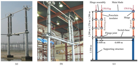
A photograph of a typical 500 kV disconnect switch assembly is shown in Figure 1a, the structural configuration of which follows the description provided above. The structural information of this disconnect switch has been reported in a previous study [18], and a shaking table test was conducted [38], as shown in Figure 1b, from which its dynamic characteristics were obtained. On this basis, a simplified numerical model of the disconnect switch was further established in the present study, as illustrated in Figure 1c. The assumptions [18] adopted in the simplified numerical model are as follows: (1) Owing to the typically irregular and serrated surface profile of porcelain insulators used in disconnect switches, detailed modeling using solid elements becomes challenging. Consequently, these solid components may be simplified as Bernoulli–Euler beam elements. Furthermore, the main blade, the base, and other components of the disconnect switch can likewise be simplified as Bernoulli–Euler beam elements. (2) The flange joint primarily consists of metallic parts and filler materials. It serves as an important connecting element in the disconnect switch by attaching a porcelain insulator to another porcelain insulator or to a supporting structure. Such a joint can be simplified as a spring with rotational stiffness. (3) A complex metallic connection structure exists between the rigid and rotating porcelain posts of the disconnect switch. For the purpose of model simplification, this structure may also be reduced to Bernoulli–Euler beam elements. (4) Porcelain insulators are brittle materials, which fail upon reaching their elastic limit during operation. Flange joints also typically exhibit a linear moment–rotation relationship. Therefore, no elastic–plastic behavior of the disconnect switch was considered in the numerical simulations. It should be noted that geometrical nonlinearities, such as large-deformation effects, and material nonlinearities of supporting structures were not considered in the present study. The results are applicable to minor or medium earthquake application scenarios, while the large earthquake scenario is only for reference.
Figure 1.
Diagram of disconnect switch, including: (a) a photograph of the actual device; (b) the experimental model in the previous study; and (c) the simplified numerical model employed in this study.
For the Bernoulli–Euler beam element, the most critical parameter is the bending stiffness , which is determined by the geometric parameters of the insulator. The rotational stiffness of the spring , on the other hand, is related to the properties of the filler material and can be expressed as [20,39,40]:
where and are the outer and inner diameters of the porcelain insulator, denotes the elastic modulus of the porcelain insulator, and are the height and thickness of the filler material used in the flange joint. and are the adjustment coefficients corresponding to the bending stiffness and the rotational stiffness , which can be determined as:
The disconnect switch was modeled in OpenSEES [41]. Bernoulli–Euler beam elements were constructed using the command “element elasticBeamColumn”, while rotational spring elements were constructed using the command “element zeroLength”. A modal analysis was performed on this simplified model, and the correctness of the model simplification was validated by comparing the results with those of shaking table tests reported in the existing literature [38]. The natural frequency measured in the shaking table test of the disconnect switch was 2.60 Hz. This frequency corresponds to the modal value of the model in the plane where the structure is located. In contrast, the modal analysis of the simplified model yielded a value of 2.70 Hz. The resulting error of 3.8% is considered to be sufficiently small, and the two sets of results can be regarded as essentially consistent. It should be noted that only a single direction along the main blade of the simplified model is considered in the seismic analysis, thus the natural frequency corresponding to this direction is employed to illustrate the modeling accuracy. If other directions of the simplified model need to be considered, more detailed comparisons of model analysis are necessary.
2.2. Earthquake Excitations and Characteristic Analysis
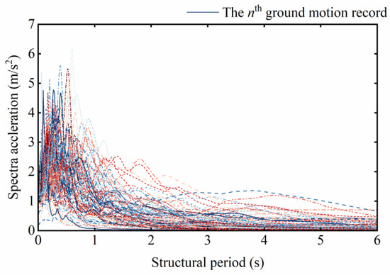
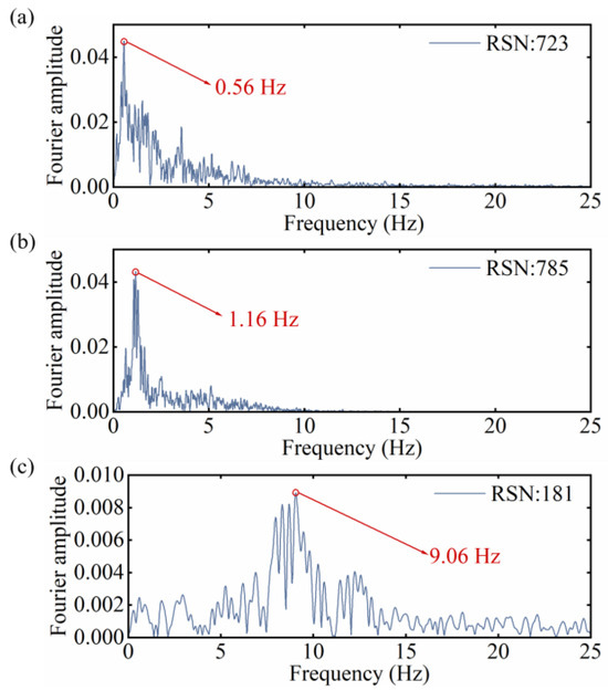
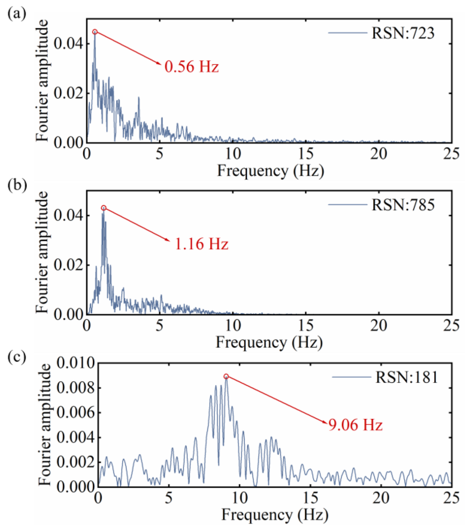
To evaluate the seismic performance [42,43,44] of the disconnect switch, a set of 102 ground motions with different dynamic characteristics was selected from the PEER ground motion database [45] as input excitations. This selection followed the guidelines of FEMA P695 [46] and previous studies [47]. They were employed as the training set in the subsequent analysis process, whose response spectra are shown in Figure 2. For the identification of their frequency characteristics, a Fast Fourier Transform [48] was first applied to the selected ground motion records, after which their frequency characteristics were obtained. Representative results of this analysis are shown in Figure 3. As can be observed from the figure, the spectral characteristics of the selected ground motions exhibit considerable variation. Specifically, the two ground motions with RSNs of 723 and 785 contain notably more low-frequency components, whereas the ground motion with an RSN of 181 is dominated by high-frequency components. The frequency characteristics of seismic waves have a substantial influence on the seismic response of the disconnect switch; therefore, the input ground motion records were first classified according to their frequency characteristics. All ground motion records were resampled with a time interval of 0.02 s, and each record was either truncated or zero-padded to a uniform length of 2500 time steps, 50 s, namely, to serve as a fixed-size input for the model training.
Figure 2.
Ground motion records employed in this study.
Figure 3.
Frequency characteristics of the employed ground motion records identified through Fast Fourier Transform analysis, including Fourier amplitude–frequency curves of earthquakes with (a) RSN:723; (b) RSN: 785; (c) RSN: 181.
In this study, the classification was performed based on the Fourier amplitude–frequency curves of the seismic waves. The frequency corresponding to the maximum Fourier amplitude was identified as the predominant frequency of each ground motion. According to this predominant frequency , the seismic waves were categorized into three categories, 1—low frequency ( Hz), 2—medium frequency ( Hz), and 3—high frequency ( Hz), which were also employed as the labels in the following seismic classification process. As can be observed from the figure, the predominant frequencies of seismic waves RSN723, RSN785, and RSN181 are 0.56 Hz, 1.16 Hz, and 9.06 Hz, respectively, which correspond to categories 1, 2, and 3, respectively.
2.3. Time History Analysis of Crucial Performance
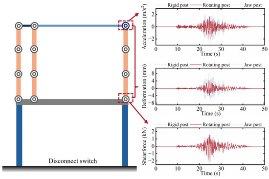
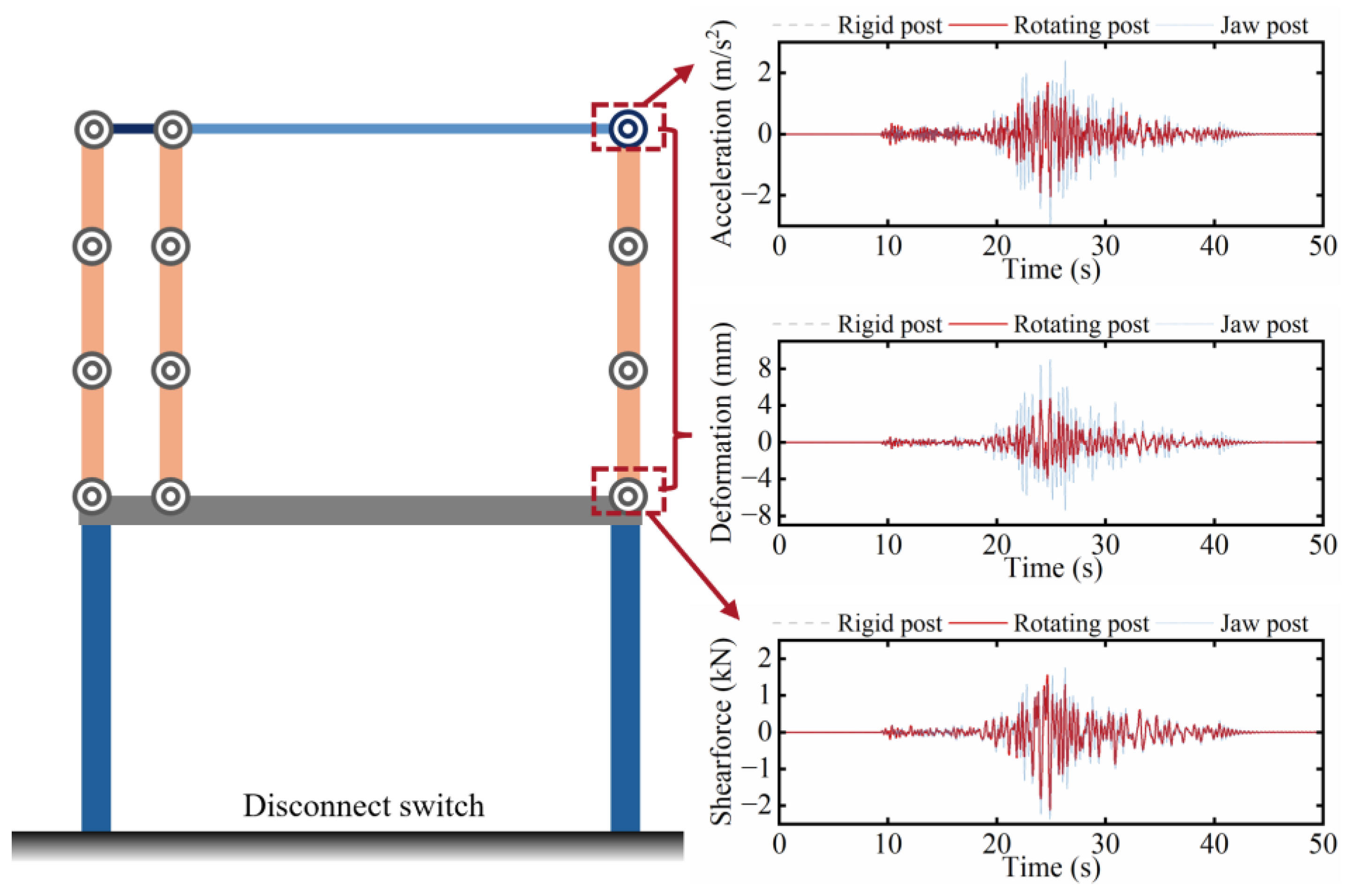
After the classification of ground motions was completed, the crucial performance indicators of the disconnect switch were further analyzed to evaluate its seismic performance. For each ground motion record, only the horizontal component was applied unidirectionally along the longitudinal axis of the disconnect switch. Vertical excitation was omitted, as it has been shown to have a negligible effect on the seismic response of slender porcelain equipment. In this study, the absolute accelerations on the top, the shear forces on the bottom, and the relative deformations between the top and bottom of the three porcelain posts were selected as the crucial performance indicators. The time history responses of these indicators were computed under the 102 ground motions, which were also employed as the training set. Among them, the computational results for the rigid post, the rotating post, and the jaw post of the disconnect switch under ground motion RSN785 are shown in Figure 4. The engineering meaning of the selected response indicators can be summarized as follows: (1) For the top absolute acceleration of porcelain post, it can be used for functionality evaluation of DS. (2) For the relative deformation between the top and bottom of a porcelain post and its bottom shear force, they are key parameters for assessing porcelain failure. (3) Furthermore, the bottom shear force also determines the demand on anchor bolts and the supporting structure.
Figure 4.
Top absolute acceleration, deformation and bottom shear force time history curves of the three posts in the disconnect switch under earthquake excitation (RSN: 785).
As can be seen from the analysis results, the time history curves of the rigid and rotating posts are almost identical, whereas those of the jaw post deviate noticeably from them. This discrepancy can be attributed to the following reasons. The metallic connection at the top of the rigid and rotating posts is relatively complex, yet the connection stiffness after simplification into Bernoulli–Euler beam element remains high, resulting in nearly identical responses of the two posts. Although the jaw post is connected to the rotating post via the main blade, the left side of the main blade is hinged to the rotating post (only the rotational degrees of freedom are released). On the right side, the blade is merely placed onto the jaw post, where not only the rotational degrees of freedom but also the horizontal degree of freedom is released, leaving only the vertical degree of freedom consistent with that of the top of the jaw post. Furthermore, the stiffness of the main blade is relatively low compared to the hinged assembled shown in Figure 1. Consequently, a substantial difference is observed between the seismic responses of the rotating post and the jaw post. In summary, the differences among the three posts are attributed to the hinge-type connection on the rotating post side and the free support on the jaw post side.
For each ground motion record shown in Figure 2, the time history responses of the crucial performance indicators of the disconnect switch were computed. On the basis of the classification of ground motions presented in the preceding section, the obtained time history responses were then divided into three datasets. In each of these datasets, the input of every sample is one-dimensional, corresponding to the time-series record of a single seismic wave, whereas the output is nine-dimensional, representing the nine dynamic time history responses of the disconnect switch.
3. Seismic Intelligent Classification and Prediction Method for DS
Based on the ground motion classification dataset and the time-series response dataset under each ground motion category established in the preceding section, a CNN can be trained to perform classification of seismic time-series data. Meanwhile, a LSTM network can be employed to learn the mapping from the time sequence of seismic waves to the crucial dynamic time-series responses of the disconnect switch, thereby enabling intelligent prediction of seismic responses. By integrating the two approaches, a CNN-LSTM-based serial seismic classification and prediction method can be formulated. In this section, the fundamental principles of CNN and LSTM, as well as the proposed method, are elaborated.
3.1. CNN-Based Seismic Classification
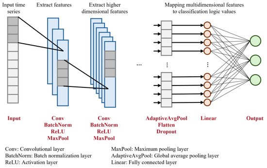
A one-dimensional convolutional neural network (1D CNN) is a special form of CNN tailored for sequence data processing. It automatically learns local waveform patterns in time series signals by sliding convolutional kernels, demonstrating unique advantages in processing time series classification tasks [34]. It can overcome the problem of hidden Markov models having difficulties with capturing long-distance correlations in time series data and solving the problems of information loss and gradient decay in recurrent neural networks. Its core principle lies in sliding one-dimensional convolution kernels along the time dimension, thereby automatically extracting local features and progressively abstracting higher-level semantic information through a hierarchical architecture. 2D CNNs are predominantly used for grid-like data such as images. In contrast, 1D CNNs are naturally suited for one-dimensional signals. These signals include time series, speech waveforms, vibration signals, bioelectric signals, and word vector sequences in natural language processing. The basic architecture of a 1D CNN typically comprises several types of layers. These include: an input layer (Input), convolutional layers (Conv), batch normalization layers (BatchNorm), activation function layers (ReLU), pooling layers (MaxPool or AdaptiveAvgPool), fully connected layers (Linear), and an output layer (Output). These layers work in concert to enable learning from raw sequences to high-level features. The model architecture is illustrated in Figure 5.
Figure 5.
Construction of the convolutional neural network to realize the frequency characteristic-based classification of ground motion records.
The input layer receives the raw one-dimensional sequence data. Suppose the input sequence has a length and a number of channels . The input layer does not perform any transformation on the data but merely serves as an interface for data entry into the network. However, normalization or standardization preprocessing is usually applied to the raw signal to accelerate training convergence and improve numerical stability. The convolutional layer is the core feature extractor of the entire network. This layer contains a number of learnable convolution kernels, each of which has a length (generally much smaller than ) and a width that matches the number of input channels . The convolution operation essentially slides the kernel along the sequence length, computing at each position the inner product between the kernel and the elements within the local receptive field, thereby generating a feature map. Following the convolutional layer, a batch normalization layer is introduced, which normalizes each batch of data to zero mean and unit variance, thereby accelerating training and allowing a higher learning rate to be used. This is immediately followed by an activation function layer to introduce nonlinear expressive capability. The most commonly used activation function is the rectified linear unit (ReLU), whose mathematical form is denoted as . The advantages of ReLU include computational simplicity, alleviation of the vanishing gradient problem, and promotion of sparse activation in the network, thereby enhancing feature discriminability. The activation function is applied element-wise to the output feature maps of the convolutional layer without altering their dimensions. The pooling layer (also referred to as a down-sampling layer) reduces the dimensionality of the feature maps along the one-dimensional direction, with max pooling being a typical operation. The pooling layer serves three main purposes. First, it reduces the temporal resolution of the feature maps, thereby decreasing the number of parameters and the computational burden in subsequent layers. Second, it enlarges the receptive field, enabling higher-layer neurons to perceive longer sequence contexts. Third, it suppresses noise and local perturbations, thereby enhancing the robustness of the model.
To improve feature extraction capability, multiple stacks of Conv-BatchNorm-ReLU-MaxPool modules are often used in a CNN. After several stages of convolution and pooling, the feature maps are compressed into a series of high-dimensional, compact feature vectors. At this point, a global average pooling layer is employed to smooth the features, substantially reducing the number of parameters in the fully connected layers and improving training efficiency. After global average pooling, the feature maps are flattened into a one-dimensional vector. A dropout layer is then applied, followed by a fully connected layer that performs an affine transformation without an activation function. For classification tasks, the last fully connected layer is followed by an output layer, in which a “softmax” function is typically used to convert the network outputs into a probability distribution, with the label having the highest probability being taken as the final output.
During forward propagation, the input sequence is denoted as , the convolution kernel , and the bias term as . The output feature map of the convolution operation at the position is given by:
With ReLU employed as the activation function, is obtained. Let the pooling window size in the pooling layer be ; then, the output feature map at the position is denoted as:
After multiple convolution operations, all feature maps are subjected to global average pooling and flattened into a vector . Denoting the weight matrix of the fully connected layer as and the bias as , the output is given by:
After passing through the “softmax” function in the output layer, the final prediction result is obtained. For the multi-classification task involved in this study, let the true label be represented as a one-hot vector and the output probability distribution of the network as . The loss is then computed as:
3.2. LSTM-Based Seismic Prediction
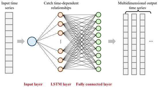
A LSTM network is a specialized recurrent neural network (RNN) architecture designed to address the vanishing and exploding gradient problems encountered by traditional RNNs when processing long sequences (Figure 6). Through the introduction of a sophisticated gating mechanism and an independent cell state, selective memory and forgetting of long-term dependencies in sequences are achieved by the LSTM, leading to widespread success in numerous sequence modeling tasks, including time-series prediction [36]. From a macro perspective, a typical LSTM network is composed of an input layer, one or more LSTM layers, and an output layer. The input layer receives the raw sequence data , where T and denote the whole time step and the input in a time step, represents the dimension of input data. The input layer is only responsible for data normalization and format conversion. The LSTM layer serves as the core processing layer, which consists of a number of LSTM units unfolded along the time axis. At each time step , a unit receives the current input , the hidden state from the previous time step , and the cell state from the previous time step , and outputs the current hidden state and the current cell state . In practical applications, multiple LSTM layers can be stacked, where the hidden state of a lower LSTM layer is used as the input to the upper LSTM layer. The LSTM layer carries all trainable parameters (weight matrices and biases for each gate). The output layer is typically a fully connected layer that maps the sequence of hidden states from all time steps onto the target space.
Figure 6.
Construction of a long short-term memory network to realize seismic response prediction of a disconnect switch.
The LSTM unit is the core of an LSTM network. A single LSTM unit contains three gating structures: the forget gate, the input gate, and the output gate, along with a cell state pathway that runs through the time axis. The forget gate determines which information is discarded from the cell state of the previous time step . A forget vector is output by this gate through a sigmoid activation function, with each component taking a value between 0 and 1, corresponding to an information channel in the cell state. A value of 1 indicates “completely retain”, while 0 indicates “completely forget”. Its calculation formula is given by
where denotes the sigmoid function, represents the weight matrix of the forget gate, denotes concatenating two vectors, and is the bias term. The input gate controls how much new information is stored into the cell state. It consists of two parts: a sigmoid gate that determines which positions to update, and a tanh layer that generates a candidate memory vector with a range between −1 and 1, which can be determined as:
where and are the weight matrices of the forget gate and candidate memory, while and are the corresponding bias terms. Under the joint action of the forget gate and the input gate, the cell state from the previous time step is updated to the cell state at the current time step as:
in which represents the element-wise product (Hadamard product). The output gate controls how much information is extracted from the current cell state as the hidden state at the current time step . First, the output gate vector is computed, and then the cell state, after being scaled by the tanh function, is multiplied by the gate value:
The hidden state serves both as the output of the current time step and as one of the inputs to the next time step. Furthermore, contains short-term dependency information, whereas assumes the role of long-term memory. Training of an LSTM is carried out using the backpropagation through time (BPTT) algorithm. During backpropagation, the error flows backwards through time and passes through the gating units. Compared with standard RNNs, the gradient path of the cell state in an LSTM involves element-wise addition and gated multiplication, which allows gradients to propagate more smoothly across time steps, effectively mitigating the vanishing gradient problem.
3.3. CNN-LSTM-Based Serial Seismic Classification and Prediction
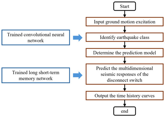
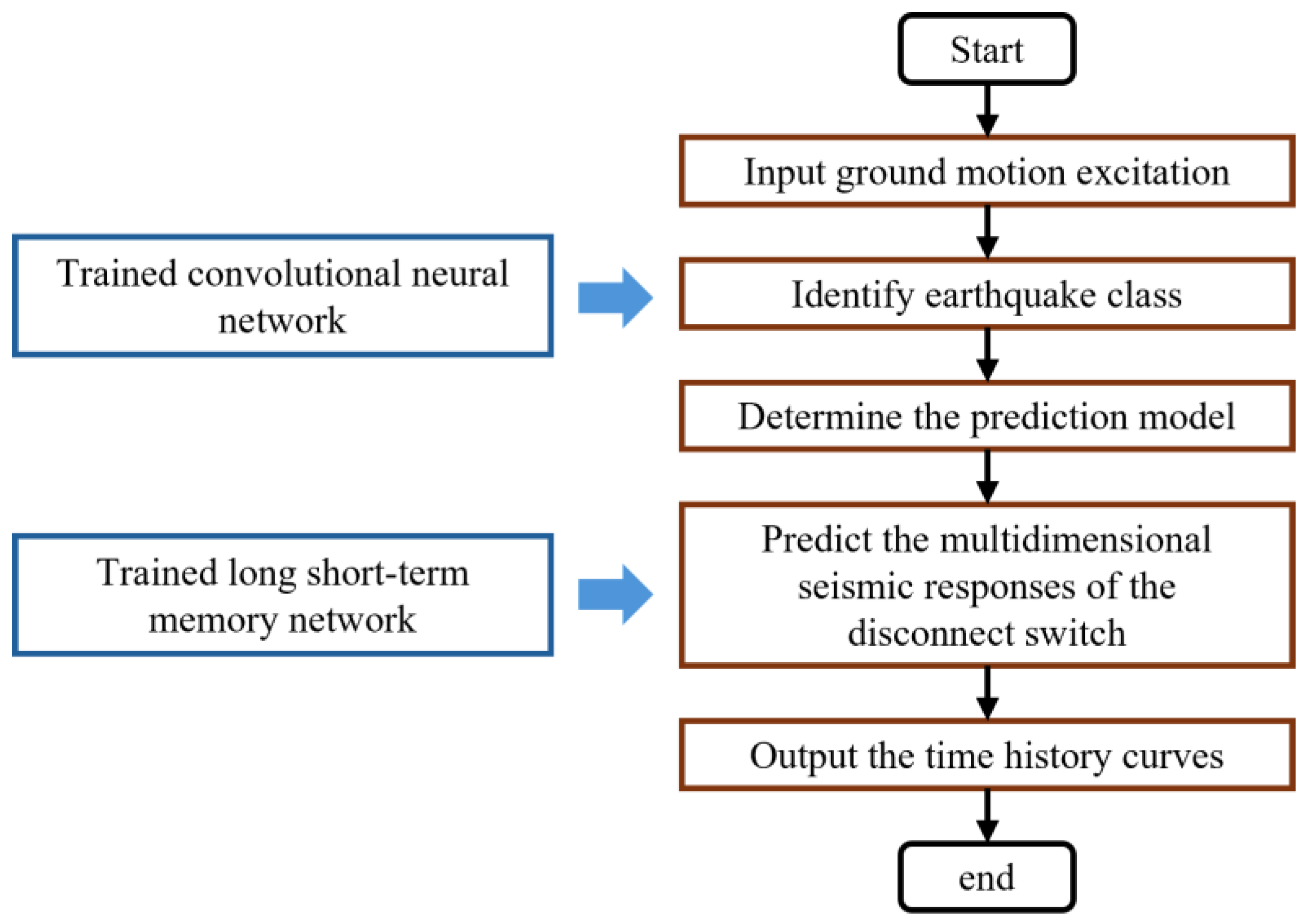
Using the dataset constructed in Section 2 as the training set, and based on the fundamental principles of CNN and LSTM networks described in Section 3.1 and Section 3.2, an intelligent classification and time-series response prediction model can be trained. By integrating these two components, the prediction flowchart shown in Figure 7 is obtained. First, a given ground motion record is taken as the input time series, and the trained CNN is used to determine the category of the ground motion record, thereby deciding which LSTM network model should be invoked for the subsequent step. Assuming that the selected ground motion record is classified as Category 1—Low frequency, the LSTM network model corresponding to Category 1 is then called to predict the time history curves of the crucial performance indicators of the disconnect switch under that earthquake.
Figure 7.
Flowchart for CNN-LSTM serial seismic classification and prediction for disconnect switch.
A standalone intelligent model can be used for prediction. Compared to that approach, the proposed CNN–LSTM serial framework exhibits the following advantage: (1) Each sub-LSTM in the framework only needs to focus on learning the response mode under a specific type of ground motion record. This leads to high internal consistency of the data and easier learning of accurate temporal features. Consequently, prediction accuracy is improved. (2) In the serial framework, the CNN classification results can directly output the type of earthquake motion, providing theoretical basis for subsequent prediction. Subsequently, each sub LSTM can independently perform feature analysis. Traditional end-to-end black box models have difficulties with providing intermediate explanations for this type of response.
4. Case Illustration
To demonstrate the effectiveness of the proposed seismic intelligent classification and prediction method, the training process of the predictive model and the hyperparameters of the trained model are presented in detail in this section. Subsequently, the prediction accuracy of the CNN model on the training set is evaluated using a confusion matrix. Using a test set distinct from the training set, the tasks of ground motion classification and response prediction are performed sequentially according to the flowchart illustrated in Figure 7. The efficiency of the proposed method in achieving rapid and intelligent prediction of the dynamic response of the disconnect switch is verified by comparing the predicted values with the true values.
During the course of this study, the model training and testing programs were developed on the Visual Studio Code 1.120 platform using the Python language. The version of Python used was 3.1.4. The machine learning models were implemented using the PyTorch library (version 2.11.0) [49], with NumPy (version 2.4.4) [50] for data processing, Matplotlib (version 3.10.9) [51] for visualization, and Scikit-learn (version 1.8.0) [52] for the confusion matrix. The device used for model training was equipped with a CPU of the type Intel(R) Core(TM) i7-14700F and a GPU of the type NVIDIA GeForce RTX 4060 Ti.
4.1. CNN Model Training and Accuracy Evaluation
The construction of the trained CNN model consisted of three Conv-BatchNorm-ReLU-MaxPool modules, followed by global average pooling and flattening. A dropout layer was added to prevent overfitting, after which a fully connected layer was attached to output the label. The construction and hyperparameters of each layer are listed in Table 1. The length of input sequence was 2500, the learning rate was set as 0.001, and the number of samples used in each training process was set as 16. The Adam optimizer [53] was employed as the learning algorithm with default parameters. A dropout rate of 0.3 was applied after the flattening layer for regularization (see Table 1). The total training dataset consisted of 102 ground motion records. For the CNN classification task, all 102 records were used for training.
Table 1.
Construction and hyperparameters of the convolutional neural network trained in this study.
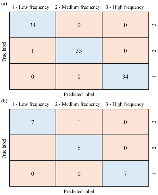
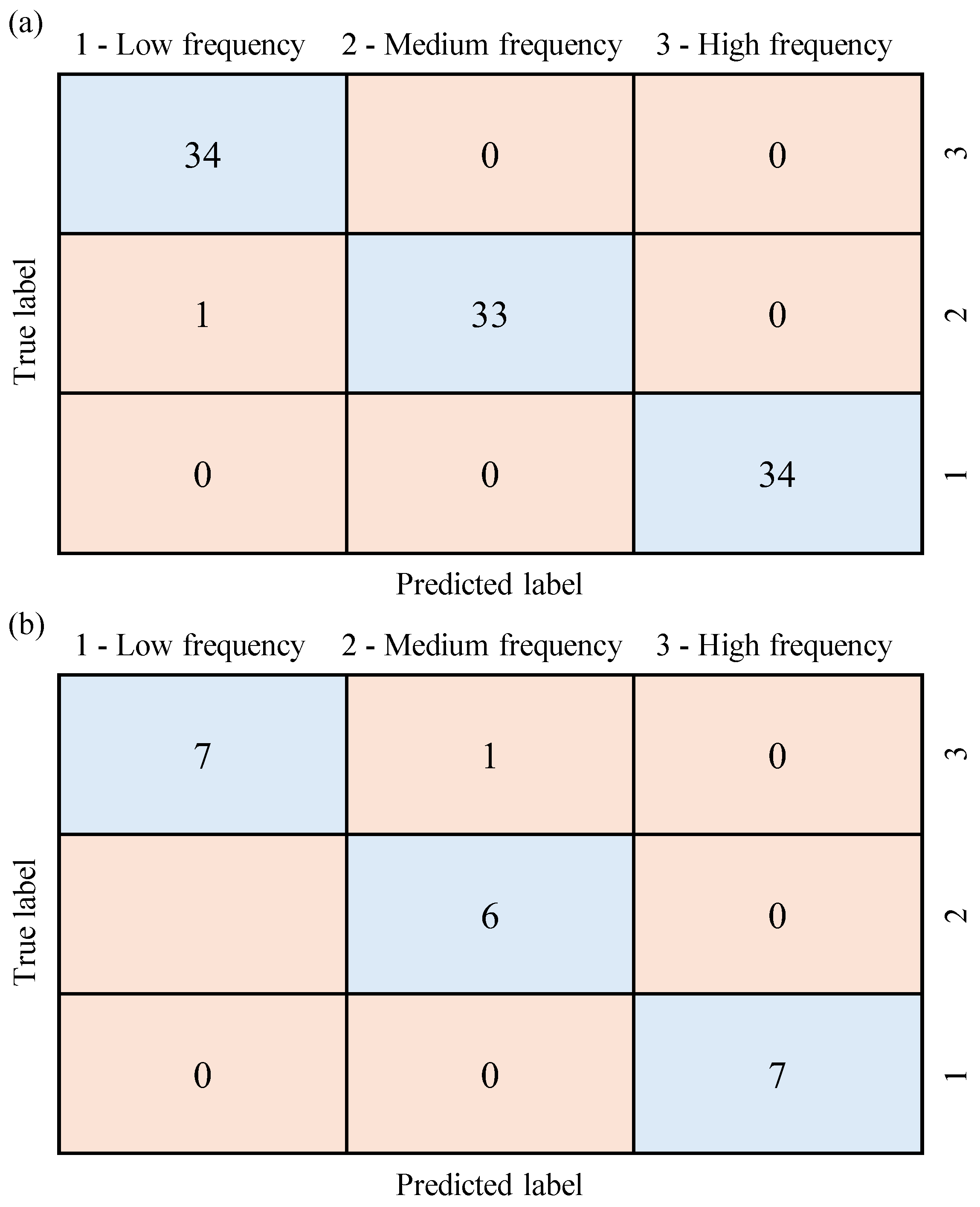
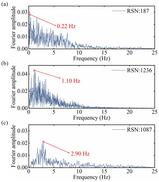
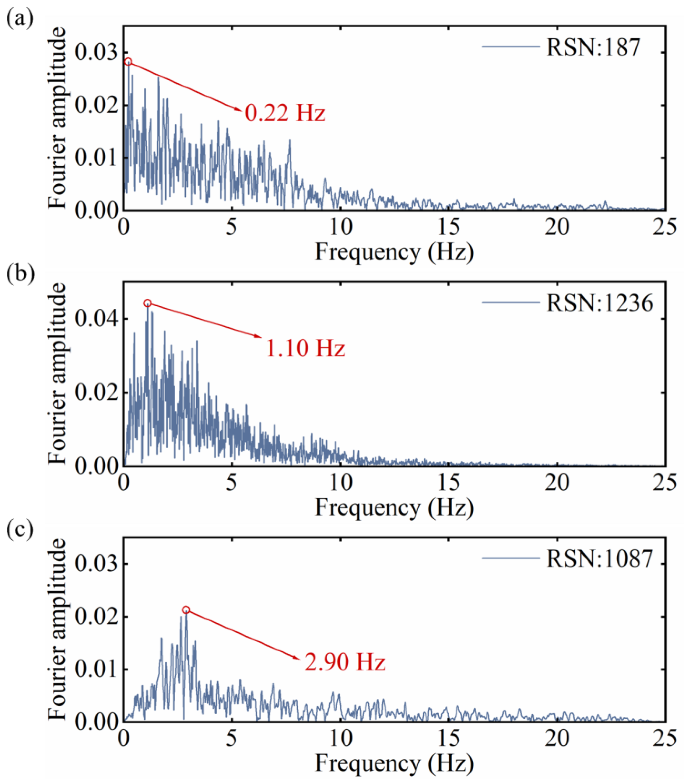
Using the trained CNN model, the predicted labels of the training set data were obtained. The confusion matrices between these predicted labels and the true labels is shown in Figure 8. As can be observed from Figure 8a, the CNN model was able to correctly classify the vast majority of ground motion records, with only one record being misclassified, yielding a prediction accuracy exceeding 99% for training dataset. In addition to the training set, ground motion records not included in the training set were also used to evaluate the prediction accuracy and generalization capability of the trained CNN model. A test set containing 21 ground motion records was employed, with a ratio of approximately 1:5 to the training set, from which the corresponding confusion matrix is illustrated in Figure 8b. It can be found that only one ground motion was misclassified, and a prediction accuracy of 95.2% was achieved, demonstrating the generalization capability of the trained model. The Fourier analysis results of the three most representative ground motion records, RSN187, RSN1236, and RSN1087, are shown in Figure 9. The frequencies corresponding to the maximum Fourier amplitude for these three waves were 0.22 Hz, 1.10 Hz, and 2.90 Hz, respectively. According to the previously established classification criteria, these indeed correspond to Categories 1, 2, and 3, respectively, indicating that the model predictions were accurate.
Figure 8.
Confusion matrices of the convolutional neural network classification results of (a) the training dataset, and (b) the testing set.
Figure 9.
Frequency characteristics of the ground motion records identified through Fast Fourier Transform analysis, including Fourier amplitude–frequency curves of earthquakes with (a) RSN:187; (b) RSN: 1236; (c) RSN: 1087.
4.2. LSTM Model Training and Accuracy Evaluation
The architecture of the trained LSTM model consisted of one LSTM layer followed by a fully connected layer, which finally output a nine-dimensional time-series response. The hyperparameters of each layer are listed in Table 2. The length of the input sequence was 2500, and the learning rate was set to 0.001. The Adam optimizer was also used for training. No dropout layer was introduced in the LSTM; instead, overfitting was mitigated by limiting the number of LSTM units to 64, which was found to provide good generalization on the validation set. Based on the ground motion classification results described above, an LSTM model was trained for each category, resulting in three models. During the training process, the 102 ground motion records were split into three training sets according to the classification results, with 34 records in each training set. For a training set corresponding to a ground motion classification, a test set with seven ground motion records was employed to demonstrate the performance of the trained model, with a ratio of approximately 1:5 to the training set.
Table 2.
Construction and hyperparameters of long short-term memory network trained in this study.
Following the workflow illustrated in Figure 7, the three exampled records, RSN187, RSN1236, and RSN1087 namely, were first classified through the models illustrated in Section 4.1. Then, different LSTM models were correspondingly selected, and the time-series responses of the key performance indicators of the DS were further predicted. Meanwhile, based on the simplified disconnect switch model described in Section 2, the actual seismic responses of the disconnect switch under the three seismic waves were computed and compared with the predictions of the LSTM models. This comparison was performed in order to evaluate the prediction accuracy and generalization capability of the trained LSTM models. In the calculation process of time history responses, calling the CNN-LSTM framework only takes 2 s to obtain the three time history curves, and the total time to load libraries such as PyTorch is also within 8 s. However, calling OpenSEES to calculate the time history curves of DS structure takes over 20 s. This indicates that using the proposed CNN-LSTM framework can greatly reduce computation time.
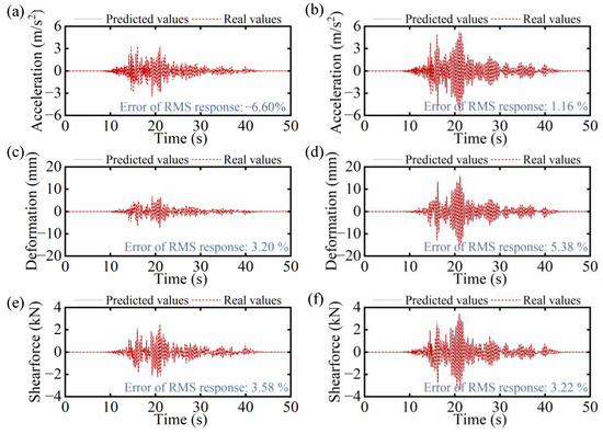
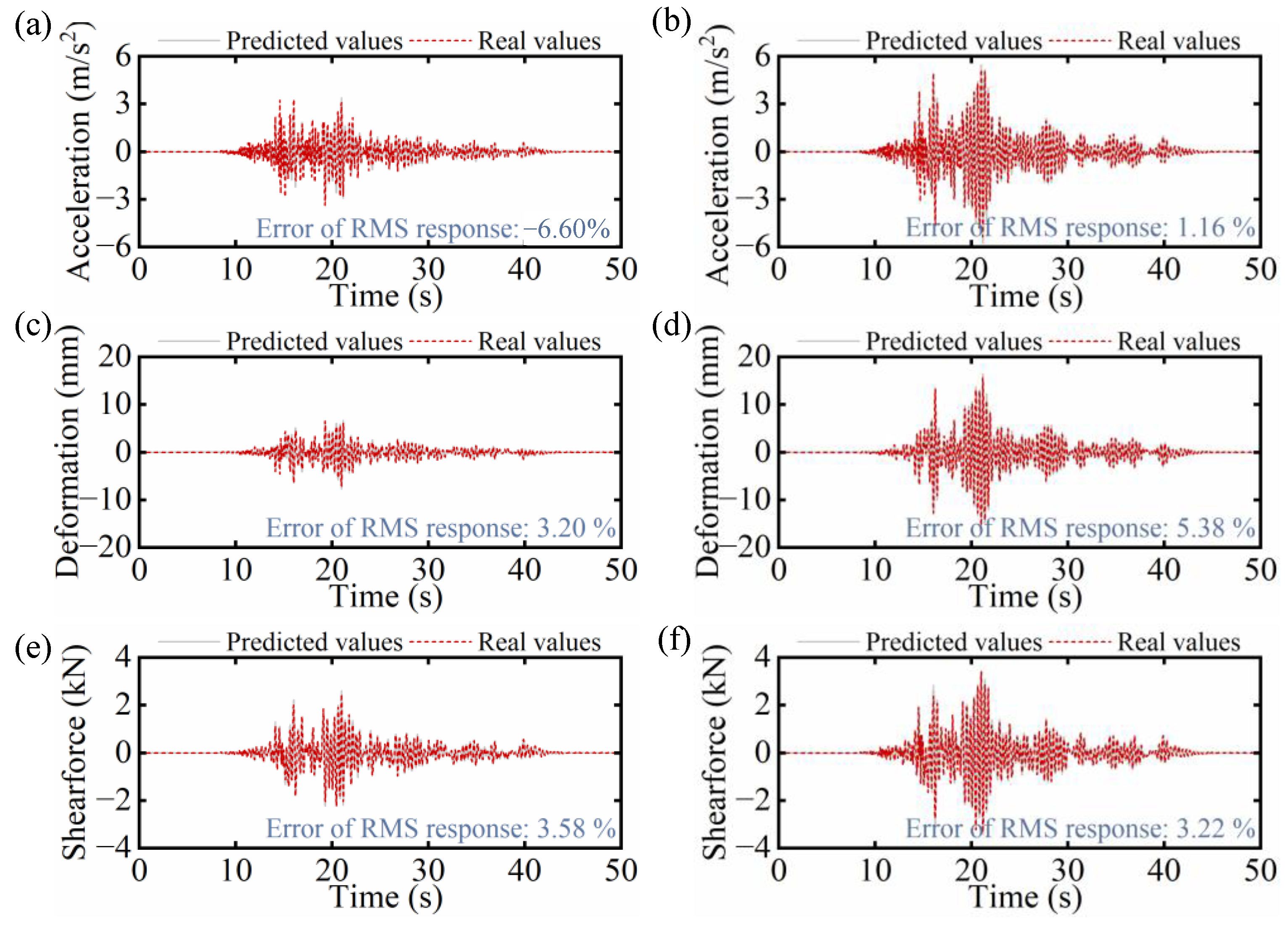
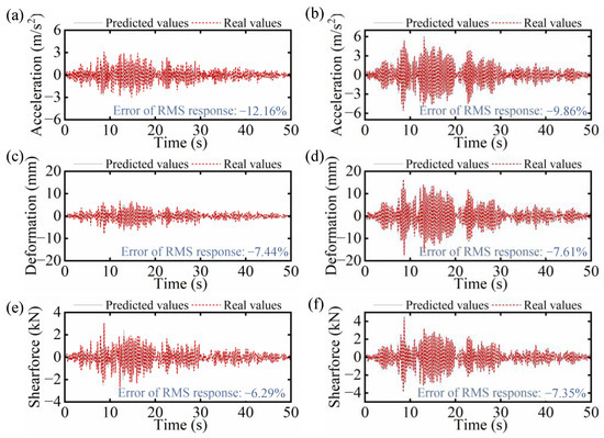
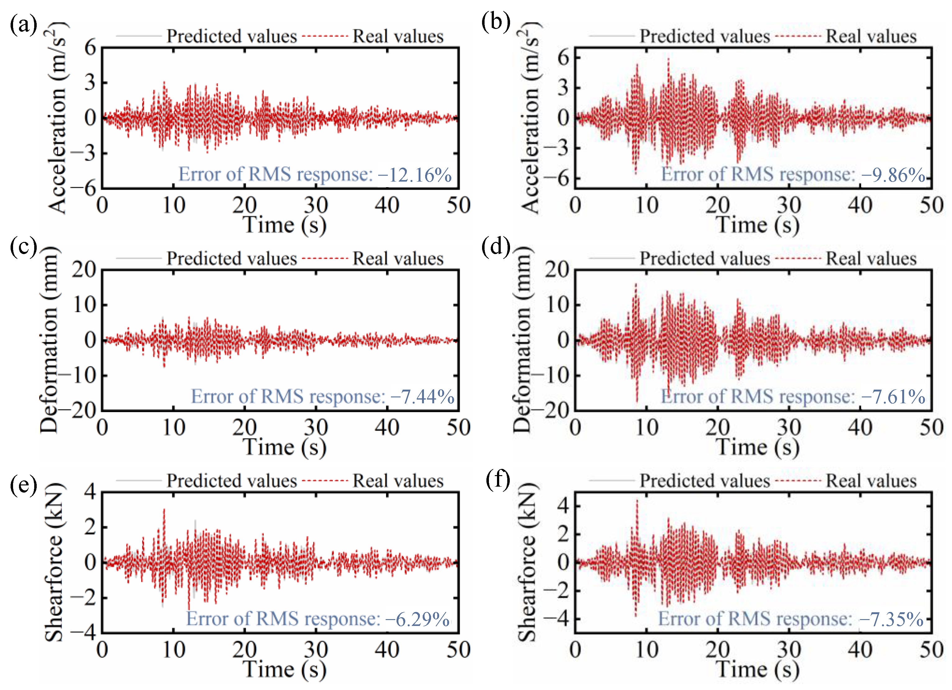
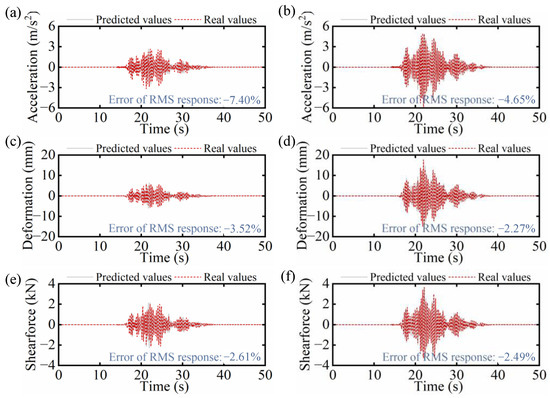
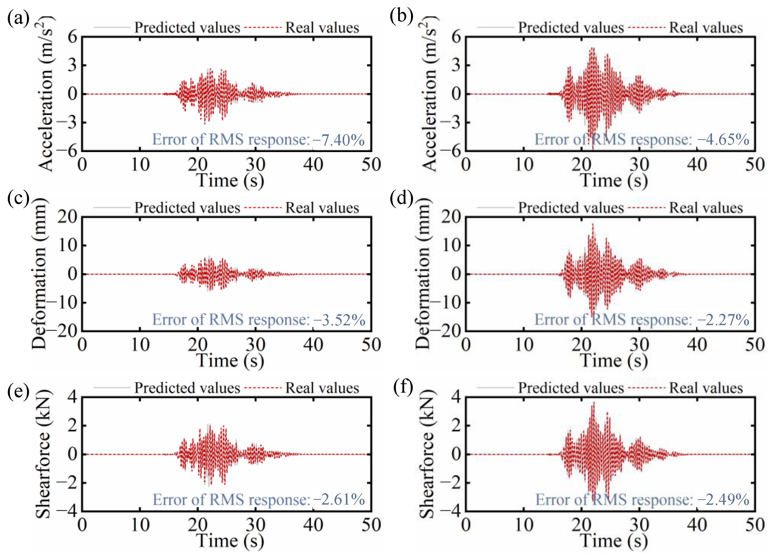
The comparison results are shown in Table 3 and Figure 10, Figure 11 and Figure 12. Under the three different earthquake records which belong to different types, the RMSE, NRMSE, MAE, R2 and Peak Error between the predicted and actual time history responses of the DS are exhibited in Table 3. It can be observed that the predictive ability of the model for acceleration response is lower than that for deformation and shear response. This may be due to the high-frequency components in the acceleration response. These high-frequency components make it difficult for the model to accurately predict the complex relationships involved. Figure 10, Figure 11 and Figure 12 directly depict and compare the predicted and actual time history curves of different dynamic responses of DS. It should be noted that, because the responses of the rigid post and the rotating post were nearly identical, only the time-history curves of the rigid post and the jaw post are presented in the figures. As can be observed from the figures, the time-series responses predicted by the LSTM models are almost completely consistent with the actually computed time-series responses, with only slight discrepancies at the peak values. Furthermore, the root-mean-square (RMS) values of the actual and predicted time history curves were first calculated, then the error between the actual and predicted RMS responses were obtained. There errors of RMS responses were generally controlled within 10%, and some results were within 3%, indicating that the LSTM models have satisfactory prediction accuracy. In addition, it can be observed that the prediction accuracy for the acceleration response was generally lower than that for the shear force and deformation responses. This may be attributed to the fact that the acceleration response contains relatively more high-frequency components, which the trained LSTM network model is currently unable to accurately characterize. Moreover, in this study, to ensure standardization of the training dataset, the selected ground motions were resampled with a time interval of 0.02 s, which to some extent also led to the loss of high-frequency components in the vibration signals.
Table 3.
Error analysis of long short-term memory network trained in this study.
Figure 10.
Comparison between predicted and real-time history curves of disconnect switch under earthquake excitation in Class 1—low frequency (RSN: 187), including: top absolute accelerations of (a) rigid post and (b) jaw post; deformations of (c) rigid post and (d) jaw post; as well as bottom shear forces of (e) rigid post and (f) jaw post.
Figure 11.
Comparison between predicted and real-time history curves of disconnect switch under earthquake excitation in Class 2—medium frequency (RSN: 1236), including: top absolute accelerations of (a) rigid post and (b) jaw post; deformations of (c) rigid post and (d) jaw post; as well as bottom shear forces of (e) rigid post and (f) jaw post.
Figure 12.
Comparison between predicted and real-time history curves of disconnect switch under earthquake excitation in Class 2—medium frequency (RSN: 1087), including: top absolute accelerations of (a) rigid post and (b) jaw post; deformations of (c) rigid post and (d) jaw post; as well as bottom shear forces of (e) rigid post and (f) jaw post.
5. Conclusions
This study proposes a CNN-LSTM-based sequential seismic classification and prediction method for the intelligent prediction of seismic responses of disconnect switches. The proposed method encompasses the model simplification strategy for the disconnect switch, the fundamental principles of the two neural networks, the training strategy, and the validation of reliability. The following conclusions are drawn:
- (1)
- A CNN-based seismic classification method is developed, which automatically learns frequency characteristics from raw ground motion records without manual feature extraction. This approach achieves an end-to-end classification accuracy exceeding 99%, overcoming the dependence of traditional rule-based classification on predefined frequency thresholds.
- (2)
- An LSTM-based prediction framework is established to map ground motion time series to the time-history responses of multiple coupled performance indicators of the disconnect switch, including accelerations, shear forces, and deformations. The multi-output architecture exploits inherent correlations among indicators, leading to improved generalization compared to single-output surrogate models.
- (3)
- Compared with conventional finite element analysis or shake table testing, the proposed hybrid CNN-LSTM method significantly reduces computational time while maintaining prediction fidelity, with root-mean-square errors generally below 10%. This enables rapid seismic performance assessment suitable for early warning or large-scale parametric studies.
- (4)
- The proposed methodology is not limited to disconnect switches; it can be extended to other slender high-voltage equipment (e.g., surge arresters, instrument transformers) and other natural hazards (e.g., strong winds, debris flows). The training and test database should also be extended to large datasets to enhance the generalization capability. Cross-validation or repeated random splitting strategies could be employed in the training process to improve the performance of model.
- (5)
- Further work will focus on experimental validation and integration into performance-based earthquake engineering or fragility analysis for power substations. The influence of geometrical and material nonlinearities should be considered under extreme ground motions. Hyperparameter optimization for the CNN and LSTM models deserves in-depth research. Comparative analysis between the proposed CNN-LSTM series framework and other models, such as standalone LSTM-, Gated Recurrent Unit-, Transformer-based methods, still needs further exploration.
Author Contributions
Y.Y. helped in conceptualization, formal analysis, writing—original draft, writing—review and editing. J.F. and G.L. contributed to formal analysis, visualization, writing—original draft, writing—review and editing. J.H. and T.M. contributed to formal analysis, visualization, writing—original draft. L.F. and M.W. helped in visualization and writing—original draft. B.Z. helped in visualization and validation. Z.Z. helped in conceptualization and validation. All authors have read and agreed to the published version of the manuscript.
Funding
This research is supported by the National Key Research and Development Program of China (Grant No. 2024YFC3015100), and Open Project Program of Shanghai Key Laboratory of Engineering Materials Application and Evaluation (Grant No. SRIM-KFKT25-05).
Data Availability Statement
Some or all data, models, or code that support the findings of this study are available from the corresponding author upon reasonable request.
Conflicts of Interest
Authors Yijun Yan, Jianhui Feng, Guobin Li, Jiang He, Teng Ma, Lina Feng were employed by the company Yunnan Power Grid Company Ltd. Author Minjun Wu was employed by the company Shanghai Key Laboratory of Engineering Materials Application and Evaluation. The remaining authors declare that the research was conducted in the absence of any commercial or financial relationships that could be construed as a potential conflict of interest.
Abbreviations
The following abbreviations are used in this manuscript:
| DS | Disconnect switch |
| CNN | Convolutional neural network |
| LSTM | Long short-term memory |
References
- Mir, F.U.H.; Yu, C.C.; Talaat, M.M.; Carmichael, B.M.; Chisholm, B.M.; Whittaker, A.S. Risk-informed, performance-based design of a seismic isolation system for a nuclear power plant. Earthq. Eng. Struct. Dyn. 2025, 54, 2231–2245. [Google Scholar] [CrossRef] [Scilit]
- Chen, N.Y.; Ji, X.Y.; Qiao, Y.K.; Hou, G.L.; Sun, L.L.; Pu, X.N.; Zhang, S.J.; Cai, X.S.; Yuan, Y. Seismic evaluation of base-isolated nuclear power plants with various tuned inerter dampers. Soil Dyn. Earthq. Eng. 2025, 197, 109438. [Google Scholar] [CrossRef] [Scilit]
- Liu, J.C.; Tian, L.; Meng, X.R.; Yang, M. Seismic fragility assessment of a transmission tower considering mainshock-aftershock sequences. J. Constr. Steel Res. 2022, 194, 107344. [Google Scholar] [CrossRef] [Scilit]
- Tian, L.; Pan, H.Y.; Ma, R.S. Probabilistic seismic demand model and fragility analysis of transmission tower subjected to near-field ground motions. J. Constr. Steel Res. 2019, 156, 266–275. [Google Scholar] [CrossRef] [Scilit]
- Tian, L.; Ma, R.S.; Qiu, C.X.; Xin, A.Q.; Pan, H.Y.; Guo, W. Influence of multi-component ground motions on seismic responses of long-span transmission tower-line system: An experimental study. Earthq. Struct. 2018, 15, 583–593. [Google Scholar]
- Luo, G.; Hu, X.W.; Bowman, E.T.; Liang, J.X. Stability evaluation and prediction of the Dongla reactivated ancient landslide as well as emergency mitigation for the Dongla Bridge. Landslides 2017, 14, 1403–1418. [Google Scholar] [CrossRef] [Scilit]
- Li, W.Z.; Cunningham, L.S.; Schultz, D.M.; Mander, S.; Gan, C.K.; Panteli, M. Structural resilience of pole-mounted substations subjected to flooding: Generalized framework and a Malaysian case study. ASCE-ASME J. Risk Uncertain. Eng. Syst. Part A Civ. Eng. 2024, 10, 04024008. [Google Scholar] [CrossRef] [Scilit]
- Zhao, Z.P.; Tang, Y.C.; Hong, N.; Chen, Q.J.; Du, Y.F. Interaction-performance-driven design of negative-stiffness friction pendulum systems for aboveground structure–connected underground structure–soil system with ground motion effects. J. Build. Eng. 2024, 88, 108970. [Google Scholar] [CrossRef] [Scilit]
- Wu, M.J.; Zhao, Z.P.; Zhang, R.F.; Zhang, B.B.; Tang, Y.C. Stability evaluation and design of negative stiffness amplifying damper-incorporated nonlinear structures. Eng. Struct. 2024, 314, 118241. [Google Scholar] [CrossRef] [Scilit]
- Zhao, Z.P.; Wang, Y.C.; Hu, X.Y.; Weng, D.G. Seismic performance upgrading of containment structures using a negative-stiffness amplification system. Eng. Struct. 2022, 260, 114394. [Google Scholar] [CrossRef] [Scilit]
- Zhao, Z.P.; Wu, M.J.; Tang, Y.C.; Weng, D.G. Adjusted energy dissipation formula and intelligent design for nonlinear negative stiffness-based amplifying damper. Eng. Struct. 2025, 329, 119849. [Google Scholar] [CrossRef] [Scilit]
- Zhao, Z.P.; Wu, M.J.; Li, Y.X.; Jiang, Y.; Hu, X.Y.; Weng, D.G. Energy dissipation enhancement of nonlinear viscous damping-integrated negative stiffness amplifying dampers. Nonlinear Dyn. 2025, 113, 7731–7758. [Google Scholar] [CrossRef] [Scilit]
- Wu, M.J.; Zhao, Z.P.; De Domenico, D.; Zhang, R.F.; Xie, M. Butterfly-shaped damping-integrated tuned viscous mass damper for highly enhanced damping and acceleration control. J. Build. Eng. 2025, 111, 113521. [Google Scholar] [CrossRef] [Scilit]
- Peker, F.U.; Yuzbasi, J.; Isik, E.; Buyuksarac, A.; Avcil, F. Damage assessment, regional ground motion record evaluation, and seismic performance analysis of a high-rise 14-story dual system building after the 2023 Kahramanmaras, earthquakes. In Structures; Elsevier: Amsterdam, The Netherlands, 2025; Volume 80, p. 109897. [Google Scholar]
- Kusky, T.M.; Bozkurt, E.; Meng, J.N.; Wang, L. Twin Earthquakes Devastate Southeast Turkiye and Syria: First Report from the Epicenters. J. Earth Sci. 2023, 34, 291–296. [Google Scholar] [CrossRef] [Scilit]
- Akar, F.; Isik, E.; Avcil, F.; Buyuksarac, A.; Arkan, E.; Izol, R. Geotechnical and Structural Damages Caused by the 2023 Kahramanmaraş Earthquakes in Gölbaşı (Adıyaman). Appl. Sci. 2024, 14, 2165. [Google Scholar] [CrossRef] [Scilit]
- Buyuksarac, A.; Avcil, F.; Alkan, H.; Isik, E.; Harirchian, E.; Ozcelik, A. Seismic Hazard Implications of the 2025 Balıkesir Earthquake of Mw 6.1 for Western Türkiye. Geohazards 2026, 6, 64. [Google Scholar]
- Delaviz, A.; Estekanchi, H.E. A rapid seismic fragility and risk analysis of electrical substation equipment considering modeling uncertainties. Eng. Struct. 2023, 293, 116686. [Google Scholar] [CrossRef] [Scilit]
- Schiff, A.J. Northridge Earthquake: Lifeline Performance and Post-Earthquake Response; Technical Council on Lifeline Earthquake Engineering: Reston, VA, USA, 1995. [Google Scholar]
- Paolacci, F.; Giannini, R.; Alessandri, S.; De Felice, G. Seismic vulnerability assessment of a high voltage disconnect switch. Soil Dyn. Earthq. Eng. 2014, 67, 198–207. [Google Scholar] [CrossRef] [Scilit]
- Paolacci, F.; Giannini, R. Seismic reliability assessment of a high-voltage disconnect switch using an effective fragility analysis. J. Earthq. Eng. 2009, 13, 217–235. [Google Scholar] [CrossRef] [Scilit]
- Xie, Q.; Zhu, R.Y.; Zhou, Y.; Yang, W.; Wang, Y.F. Shake table test on 220 kV disconnecting switch. Power Syst. Tech. 2012, 36, 262–267. [Google Scholar]
- Wen, B.; Moustafa, M.A.; Dai, J.W. Seismic fragilities of high-voltage substation disconnect switches. Earthq. Spectra 2019, 35, 1559–1582. [Google Scholar] [CrossRef] [Scilit]
- Whittaker, A.S.; Fenves, G.L.; Gilani, A.S.J. Seismic evaluation and analysis of high-voltage substation disconnect switches. Eng. Struct. 2007, 29, 3538–3549. [Google Scholar] [CrossRef] [Scilit]
- Moustafa, M.A.; Mosalam, K.M. Substructured dynamic testing of substation disconnect switches. Earthq. Spectra 2016, 32, 567–589. [Google Scholar] [CrossRef] [Scilit]
- Bastami, M.; Hajihasani, M. Input waves for seismic design of power substation equipment for near and far Iranian earthquake records. Int. J. Civ. Eng. 2014, 12, 55–72. [Google Scholar]
- Qin, S.Z.; Fei, Y.F.; Liao, W.J.; Lu, X.Z. Leveraging data-driven artificial intelligence in optimization design for building structures: A review. Eng. Struct. 2025, 341, 120810. [Google Scholar] [CrossRef] [Scilit]
- Lazaridis, P.C.; Kavvadias, I.E.; Demertzis, K.; Iliadis, L.; Vasiliadis, L.K. Structural damage prediction of a reinforced concrete frame under single and multiple seismic events using machine learning algorithms. Appl. Sci. 2022, 12, 3845. [Google Scholar] [CrossRef] [Scilit]
- Wei, X.X.; Fu, B.; Wu, W.Y.; Liu, X.R. Effects of vertical ground motion on pedestrian-induced vibrations of footbridges: Numerical analysis and machine learning-based prediction. Buildings 2022, 12, 2138. [Google Scholar] [CrossRef] [Scilit]
- Mor, B.; Garhwal, S.; Kumar, A. A systematic review of hidden Markov models and their applications. Arch. Comput. Method. Eng. 2021, 28, 1429–1448. [Google Scholar] [CrossRef] [Scilit]
- Michelot, T.; Langrock, R.; Patterson, T.A. moveHMM: An R package for the statistical modelling of animal movement data using hidden Markov models. Methods Ecol. Evol. 2016, 7, 1308–1315. [Google Scholar] [CrossRef] [Scilit]
- Huang, L.L.; Park, J.H.; Wu, G.C.; Mo, Z.W. Variable-order fractional discrete-time recurrent neural networks. J. Comput. Appl. Math. 2020, 370, 112633. [Google Scholar] [CrossRef] [Scilit]
- Yu, Y.; Si, X.S.; Hu, C.H.; Zhang, J.X. A Review of Recurrent Neural Networks: LSTM Cells and Network Architectures. Neural Comput. 2019, 31, 1235–1270. [Google Scholar] [CrossRef] [Scilit] [PubMed]
- Gu, J.X.; Wang, Z.H.; Kuen, J.; Ma, L.Y.; Shahroudy, A.; Shuai, B.; Liu, T.; Wang, X.X.; Wang, G.; Cai, J.F.; et al. Recent advances in convolutional neural networks. Pattern Recognit. 2018, 77, 354–377. [Google Scholar] [CrossRef] [Scilit]
- ArunKumar, K.E.; Kalaga, D.V.; Kumar, C.M.S.M.; Kawaji, M.; Brenza, T.M. Comparative analysis of Gated Recurrent Units (GRU), long Short-Term memory (LSTM) cells, autoregressive Integrated moving average (ARIMA), seasonal autoregressive Integrated moving average (SARIMA) for forecasting COVID-19 trends. Alex. Eng. J. 2022, 61, 7585–7603. [Google Scholar] [CrossRef] [Scilit]
- Van Houdt, G.; Mosquera, C.; Napoles, G. A review on the long short-term memory model. Artif. Intell. Rev. 2020, 53, 5929–5955. [Google Scholar] [CrossRef] [Scilit]
- Liao, L.Y.; Zhou, H.L.; Liu, J.P.; Zhou, J.; Zhang, D.H.; Wang, J. A PSO-CNN-LSTM model for seismic facies analysis: Methodology and applications. IEEE Access 2025, 13, 84094–84111. [Google Scholar] [CrossRef] [Scilit]
- Takhirov, S.; Fenves, G.L.; Fujisaki, E. Seismic Qualification and Fragility Testing of Line Break 550-kV Disconnect Switches; PEER Report; Pacific Earthquake Engineering Research Center: Berkeley, CA, USA, 2005. [Google Scholar]
- Alessandri, S.; Giannini, R.; Paolacci, F.; Malena, M. Seismic retrofitting of an HV circuit breaker using base isolation with wire ropes. Part 1: Preliminary tests and analyses. Eng. Struct. 2015, 98, 251–262. [Google Scholar] [CrossRef] [Scilit]
- Moustafa, M.A.; Mosalam, K.M. Structural performance of porcelain and polymer post insulators in high voltage electrical switches. J. Perform. Constr. Facil. 2016, 30, 04016002. [Google Scholar] [CrossRef] [Scilit]
- McKenna, F.; Fenves, G.L.; Scott, M.H. Open System for Earthquake Engineering Simulation; Pacific Earthquake Engineering Research Center: Berkeley, CA, USA, 2003. [Google Scholar]
- Wu, M.J.; Zhao, Z.P.; Zong, G.; Yang, K.; Zhang, B.B. Spectral acceleration-based design methodology of tuned viscous mass damper-integrated frame structures. J. Build. Eng. 2026, 125, 116134. [Google Scholar] [CrossRef] [Scilit]
- Tang, Y.C.; Zhao, Z.P.; Li, Y.X.; Wang, L.; Chen, Q.J. Interaction evaluation and adjusted design of negative-stiffness friction pendulum systems for aboveground-underground connected system with adjacent aboveground structures. Eng. Struct. 2025, 343, 121101. [Google Scholar] [CrossRef] [Scilit]
- Zhao, Z.P.; Tang, Y.C.; Chen, Q.J.; Wu, M.J.; Jiang, Y. Resilient slip-friction connection-enhanced self-centering column for the low-damage prefabricated underground structures. Tunn. Undergr. Space Technol. 2025, 164, 106776. [Google Scholar] [CrossRef] [Scilit]
- University of California, Berkeley. PEER Ground Motion Database. Pacific Earthquake Engineering Research Center. Available online: https://ngawest2.berkeley.edu/ (accessed on 19 April 2026).
- FEMA. Quantification of Building Seismic Performance Factors; FEMA P-695; Applied Technology Council for the Federal Emercency Management Agency: Redwood City, CA, USA, 2009. [Google Scholar]
- Hong, N.; Zhao, Z.P.; Du, Y.F.; Chen, Q.J. Energy spectra and performance assessment of isolated structures with a negative stiffness amplification system. Soil. Dyn. Earthq. Eng. 2023, 169, 107857. [Google Scholar] [CrossRef] [Scilit]
- Chopra, A.K. Dynamics of Structures: Theory and Applications to Earthquake Engineering, 4th ed.; Prentice Hall: Hoboken, NJ, USA, 2012. [Google Scholar]
- Paszke, A.; Gross, S.; Massa, F.; Lerer, A.; Bradbury, J.; Chanan, G.; Killeen, T.; Lin, Z.M.; Gimelshein, N.; Antiga, L.; et al. PyTorch: An Imperative Style, High-Performance Deep Learning Library. In Proceedings of the 33rd Conference on Neural Information Processing Systems (NeurIPS), Vancouver, BC, Canada, 8–14 December 2019. [Google Scholar]
- Harris, C.R.; Millman, K.J.; van der Walt, S.J.; Gommers, R.; Virtanen, P.; Cournapeau, D.; Wieser, E.; Taylor, J.; Berg, S.; Smith, N.J.; et al. Array programming with NumPy. Nature 2020, 585, 357–362. [Google Scholar] [CrossRef] [Scilit]
- Hunter, J.D. Matplotlib: A 2D graphics environment. Comput. Sci. Eng. 2007, 9, 90–95. [Google Scholar] [CrossRef] [Scilit]
- Pedregosa, F.; Varoquaux, G.; Gramfort, A.; Michel, V.; Thirion, B.; Grisel, O.; Blondel, M.; Prettenhofer, P.; Weiss, R.; Dubourg, V.; et al. Scikit-learn: Machine Learning in Python. J. Mach. Learn. Res. 2011, 12, 2825–2830. [Google Scholar]
- Kingma, D.P.; Ba, J. Adam: A Method for Stochastic Optimization. In Proceedings of the 3rd International Conference on Learning Representations, San Diego, CA, USA, 7–9 May 2015. [Google Scholar]

Disclaimer/Publisher’s Note: The statements, opinions and data contained in all publications are solely those of the individual author(s) and contributor(s) and not of MDPI and/or the editor(s). MDPI and/or the editor(s) disclaim responsibility for any injury to people or property resulting from any ideas, methods, instructions or products referred to in the content. |
© 2026 by the authors. Licensee MDPI, Basel, Switzerland. This article is an open access article distributed under the terms and conditions of the Creative Commons Attribution (CC BY) license.