Rapid Prediction of Side Ledge Morphology and Thermal Fields in Aluminum Reduction Cells via CFD-Based Machine Learning

Abstract

The side ledge is essential for maintaining thermal stability and protecting the sidewall lining in an aluminum reduction cell. Its shape and temperature distribution strongly influence cell operation and energy efficiency. However, conventional computational fluid dynamics (CFD) methods, while accurate, are computationally intensive and unsuitable for fast evaluation under changing operating conditions. To overcome this limitation, this study develops a CFD-driven machine learning surrogate model for rapid prediction of cross-sectional temperature fields and side ledge morphology in an aluminum reduction cell under magnetohydrodynamic (MHD) conditions. High-fidelity training data are first generated from MHD-CFD simulations. Key physical variables, including heat generation, effective thermal transport properties, and velocity components, are extracted from multiple cross-sections prior to side ledge formation to form the input dataset. Five machine learning methods—Decision Tree, Random Forest, XGBoost, K-Nearest Neighbors, and Support Vector Regression—are then developed to predict the resulting temperature field and side ledge profile after solidification. The performance of each model is systematically compared in terms of accuracy and applicability. Among the tested models, Random Forest demonstrates the best overall performance. Its predicted temperature fields closely match CFD results, with a maximum temperature deviation below 0.23 °C, while the average side ledge thickness error is only 0.0153 m. Moreover, the proposed surrogate model reduces computation time from approximately 168 h to 3 min compared with CFD simulations, while maintaining high predictive accuracy. Overall, the proposed method enables fast and accurate evaluation of thermal states, supports operational optimization, and provides a foundation for digital twin development of aluminum reduction cells.

1. Introduction

The aluminum electrolysis industry is one of the most energy-intensive metallurgical sectors, where the operational stability and energy efficiency of the aluminum reduction cell directly affect production costs and carbon emissions [1]. Along the cell sidewall, the side ledge, formed by the solidification of molten electrolyte, acts as a critical thermo-structural protective layer. Its thickness, toe length, and spatial distribution strongly influence the cell thermal balance, the protection of the sidewall lining, and the stability of the electrolysis process [2]. The side ledge is a dynamic interface whose morphology continuously evolves under coupled electrical, magnetohydrodynamic (MHD), and thermal fields within the cell. Deviations from its desired profile can disrupt the thermal balance, leading to local overheating, accelerated lining degradation, and, in severe cases, sidewall burn-through or metal leakage [3]. Maintaining a stable side ledge is therefore essential for the safe and efficient operation of aluminum reduction cells. Despite its importance, direct observation of the side ledge remains extremely challenging. Aluminum reduction cells operate at temperatures of approximately 930–970 °C in a highly corrosive molten electrolyte under strong electromagnetic fields. Moreover, the enclosed and opaque cell structure prevents continuous and full-field measurements of key state variables, including side ledge morphology and the internal temperature distribution, using conventional experimental techniques [4]. Consequently, studies of side ledge formation and evolution have relied primarily on numerical simulation strategies to investigate the underlying physical mechanisms [5].

Computational Fluid Dynamics (CFD) reconstructs molten bath flow and heat transfer by numerically solving the governing equations, making it a fundamental tool for investigating side ledge formation and evolution [6]. By predicting the temperature and flow fields within an aluminum reduction cell, CFD enables detailed analysis of side ledge morphology and its influence on cell performance [7]. Over the past decades, CFD models for aluminum reduction cells have evolved from simplified heat conduction models [8,9,10] to comprehensive multiphysics simulations [11,12,13,14]. Early studies primarily employed steady-state heat conduction or weakly coupled flow–heat transfer models, in which electromagnetic effects were either neglected or represented as body force terms to examine side ledge formation [15,16]. To better capture the influence of electric current and magnetic fields on molten bath flow, subsequent models incorporated electromagnetic body forces, resulting in coupled electro–magnetic–flow simulations with improved predictions of flow and heat transfer [17]. More recently, strongly coupled MHD models have enabled the simultaneous solution of the electric, magnetic, flow, and thermal fields, providing a more accurate representation of the multiphysics interactions within aluminum reduction cells [18]. Consequently, CFD/MHD models have become the primary numerical approach for studying the thermal behavior of aluminum reduction cells and the evolution of the side ledge.

Despite their high predictive accuracy, CFD/MHD models remain computationally expensive. Because they rely on solving fully coupled governing equations, any change in operating conditions or boundary parameters requires a new simulation to predict the corresponding temperature field and side ledge morphology. This computational burden limits their applicability to rapid process evaluation and real-time industrial decision-making. Moreover, accurate side ledge prediction requires reconstructing high-dimensional spatial temperature fields with strong nonlinear and multiphysics characteristics, further increasing the computational complexity. These limitations motivate the development of more efficient predictive strategies capable of delivering accurate results with substantially lower computational cost.

To overcome the computational limitations of high-fidelity numerical simulations, machine learning (ML)-based surrogate models have emerged as an effective approach for the rapid prediction of complex engineering systems [19]. By learning the nonlinear mapping between input variables and target outputs, these models can accurately approximate simulation results without repeatedly solving the governing equations, substantially reducing computational cost. A range of ML algorithms, including Random Forest (RF), Support Vector Regression (SVR), Extreme Gradient Boosting (XGBoost), and Artificial Neural Networks (ANNs), have been successfully applied to replace computationally intensive CFD simulations in flow reconstruction and temperature prediction tasks [20,21,22,23,24,25]. In aluminum reduction cells, however, existing ML studies have focused primarily on scalar quantities, such as cell voltage and energy consumption. Comparatively few studies have addressed the reconstruction of spatial temperature fields or the prediction of side ledge morphology. Moreover, spatial surrogate models trained on high-fidelity CFD/MHD simulation data remain largely unexplored. These research gaps underscore the need for efficient ML-based strategies capable of accurately reconstructing complex thermal fields and predicting side ledge evolution in aluminum reduction cells. Such approaches can retain the predictive capability of high-fidelity simulations while providing the computational efficiency required for rapid evaluation and real-time industrial applications.

To address the above challenges, this study proposes a CFD-driven machine learning surrogate modeling framework for the rapid reconstruction of the temperature field and side ledge morphology in an aluminum reduction cell. First, based on the results of coupled thermal–electrical–magnetohydrodynamic (MHD) CFD simulations, key local physical quantities, including Joule heat, equivalent thermal conductivity, and the three velocity components, were extracted from different spatial cross-sections within the molten electrolyte region to construct a high-fidelity dataset. The spatial coordinates of the nodes were used only to establish the correspondence between different cross-sections and to reconstruct the predicted temperature field, rather than as input features to the machine learning models. Unlike conventional surrogate models that predict only the average temperature, temperatures at limited measurement locations, or global thermal balance parameters, the proposed approach predicts the complete temperature distribution over an entire cross-section. The predicted temperature field is then used to identify the side ledge boundary, enabling the rapid reconstruction of the side ledge thickness and morphology. Subsequently, five machine learning models—Decision Tree (DT), Random Forest (RF), Extreme Gradient Boosting (XGBoost), K-Nearest Neighbors (KNN), and Support Vector Regression (SVR)—were systematically evaluated using the same CFD-generated dataset, identical training–testing data partition, and consistent evaluation metrics. Their performance was compared in terms of cross-sectional temperature field prediction, spatial field reconstruction, and computational efficiency. The primary contribution of this work is the development of a CFD–machine learning framework for reconstructing the thermal field and side ledge morphology of an aluminum reduction cell, rather than the proposal of a new machine learning algorithm. After the offline CFD/MHD simulations and model training have been completed, the trained surrogate model can rapidly predict the temperature field and side ledge morphology of previously unseen cross-sections under the same operating condition, without requiring additional CFD simulations. This framework provides a methodological basis for rapid thermal state assessment and field reconstruction in future digital twin applications for aluminum reduction cells.

2. Methodology

2.1. Data Preprocessing

The CFD simulations were performed using ANSYS Fluent 2022 R1. The machine learning models were implemented in Python 3.10. Decision Tree (DT), Random Forest (RF), K-Nearest Neighbors (KNN), and Support Vector Regression (SVR) were implemented using the scikit-learn library, whereas XGBoost was implemented using the XGBoost Python library. Data preprocessing, model training, and the interface between the CFD results and the machine learning models were developed in Python. All computations were carried out on the same workstation running Microsoft Windows 10 (64-bit), equipped with dual AMD EPYC 7R32 processors, 256 GB RAM, and an NVIDIA GeForce RTX 3090 GPU. The detailed CFD modeling approach and parameter settings are provided in a previous study [18]. In this work, magnetic field effects were applied using the built-in MHD module in Fluent 2022 R1. The simulation was carried out in two stages. First, a steady-state solution was obtained without side ledge formation to establish the flow and electromagnetic fields. Then, the assumption of constant temperature in the molten electrolyte was removed, and a transient simulation was performed until the side ledge geometry reached a stable state. The convergence criteria for both the flow field and side ledge evolution follow those defined in [18].

Because the physical fields exhibit significant spatial non-uniformity, the temperature distribution and side ledge profile differ considerably between cross-sections perpendicular to the X-axis (X-planes) from the current inlet side to the current outlet side of the aluminum reduction cell. To characterize this spatial variation while considering the large geometric dimension of the cell along the X-direction (17.812 m), consecutive adjacent cross-sections were not used as data samples. Instead, cross-sections were extracted at approximately 0.27 m intervals along the X-direction. This sampling strategy ensures adequate spatial coverage of different regions of the cell while reducing the strong spatial correlation between neighboring cross-sections that could otherwise bias the evaluation of the machine learning models.

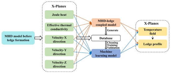
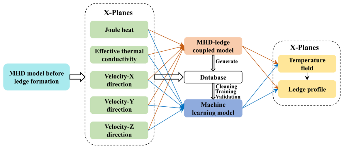
A total of 128 cross-sections were extracted from both sides of the cell. For each cross-section, Joule heat, equivalent thermal conductivity, and the three velocity components at each mesh node before side ledge formation were extracted as the five input features of the machine learning models, whereas the nodal temperature after side ledge formation at the corresponding node was used as the prediction target. After predicting the complete nodal temperature field of a cross-section, the side ledge boundary was identified according to the predicted temperature distribution and the corresponding criterion, thereby reconstructing the side ledge morphology. Based on this procedure, a CFD-generated database was established for subsequent machine learning model training and prediction. The overall workflow is illustrated in Figure 1.

Figure 1. Workflow of the proposed framework for rapid prediction of local molten bath temperature and side ledge morphology under MHD-coupled conditions.

According to the unified mesh discretization, each cross-section perpendicular to the X-axis contains 1432 nodes within the molten electrolyte region. Consequently, the 128 cross-sections generate 183,296 node-level samples, resulting in an input matrix of 183,296 × 5 and an output temperature vector of 183,296 × 1. All cross-sections share the same mesh topology and node numbering scheme. The Y and Z coordinates were used only to establish the correspondence of nodes among different cross-sections and to reconstruct the predicted temperature field, and were not included as input features of the machine learning models. Although the spatial coordinates were not used as input variables, the selected physical features—namely Joule heat, equivalent thermal conductivity, and the three velocity components—exhibit inherent spatial distributions and therefore implicitly characterize the local physical state of each node. Subsequently, both the input features and the output temperature were normalized prior to model training. The detailed data structure is summarized in Table 1 and Table 2.

Table 1. Sample input feature dataset for a molten bath cross-section.

Node No.	Y (m)	Z (m)	Effective Thermal Conductivity (W·m−1·K−1)	Joule Heat (W·m−3)	Velocity-X (m·s−1)	Velocity-Y (m·s−1)	Velocity-Z (m·s−1)
0	1.3933	0.8880	163.9983	78.4558	0.1124	0.0155	0.0002
1	1.4500	0.8880	169.4365	79.1734	0.1234	0.0201	−0.0001
…	…	…	…	…	…	…	…
1431	2.0700	1.2770	101.0495	5.18501	0.1018	−0.0222	0.0000

Table 2. Sample output dataset for a molten bath cross-section.

Node No.	Y (m)	Z (m)	Temperature (°C)
0	1.3933	0.8880	946.5103
1	1.4500	0.8880	946.6960
…	…	…	…
1431	2.0700	1.2770	280.1550

To avoid overly optimistic performance estimates arising from spatial correlation, the dataset was partitioned using complete cross-sections rather than randomly selected mesh nodes. Specifically, 80% of the cross-sections were used for training and the remaining 20% for testing. Consequently, no cross-section appeared in both the training and test sets, and the evaluation therefore reflects the model’s ability to reconstruct the temperature field of previously unseen cross-sections under the same operating condition, rather than its ability to interpolate among neighboring nodes.

2.2. Feature Correlation Analysis

To analyze the interdependencies among the input feature variables and reduce the potential impact of redundant information between features on the prediction performance of the model, the Mutual Information (MI) method was adopted to evaluate the degree of association among different feature variables. Mutual information can quantify the statistical dependence between two variables. Unlike traditional correlation analysis, it can characterize not only linear relationships but also effectively capture nonlinear dependencies between variables. Its calculation is expressed as follows:

$$I(X;Y)={\sum }_{x\in X} {\sum }_{y\in Y} p(x,y)\mathrm{l}\mathrm{o}\mathrm{g}{\displaystyle \frac{p(x,y)}{p(x)p(y)}}$$

(1)

where I(X;Y) represents the mutual information between variables X and Y, p(x,y)denotes the joint probability distribution, and p(x) and p(y) represent the marginal probability distributions of variables X and Y, respectively. A larger mutual information value indicates that the two variables share more common information and exhibit stronger correlations. When the mutual information value approaches zero, the variables exhibit weak statistical dependence.

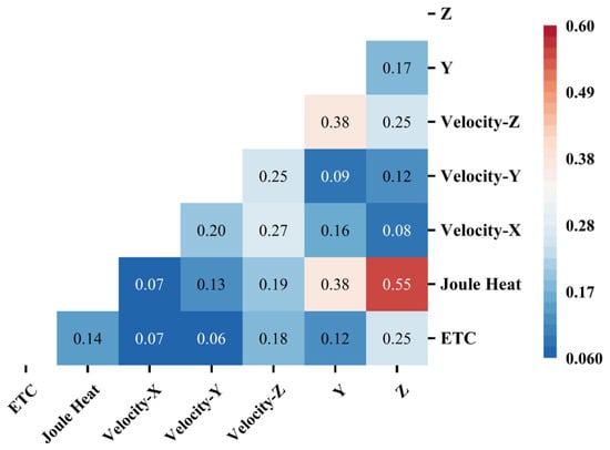
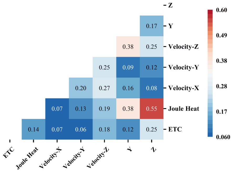
Figure 2 presents the mutual information matrix among the seven feature variables used for predicting the side ledge and temperature distribution in the aluminum reduction cell. As shown in the figure, the mutual information values among most feature variables are relatively low, indicating that the selected input variables do not exhibit significant information redundancy. Among them, the mutual information value between Joule heat and the Z-axis coordinate is the highest, reaching 0.55, suggesting a relatively strong information correlation between these two variables. This phenomenon is mainly attributed to the fact that Joule heat generation in the molten region is closely related to spatial position. In particular, near the interpolar region, the non-uniform distribution of current density results in localized Joule heat concentration, causing Joule heat to exhibit a certain spatial variation pattern along the Z direction. In addition, the mutual information values between Joule heat and the Y-axis coordinate, as well as between Velocity-Z and the Y-axis coordinate, are both 0.38, indicating a certain degree of dependence among these variables. This observation is consistent with the physical characteristics that heat distribution and flow behavior inside the molten region are affected by spatial locations. In contrast, the mutual information values among effective thermal conductivity(ETC), velocity components in different directions, and other spatial variables are relatively low, with most values below 0.30, demonstrating good independence among these feature variables. Overall, although Joule heat and the Z-axis coordinate exhibit a relatively high mutual information value, they represent different physical meanings, corresponding to heat source distribution characteristics and spatial position information, respectively, rather than completely redundant variables. Therefore, retaining all input features enables the prediction model to fully learn the complex nonlinear relationships among the thermal field, flow field, and spatial position, thereby improving the prediction accuracy of the side ledge and temperature distribution.

Figure 2. Mutual information matrix among the input feature variables.

2.3. Machine Learning Model Selection

The prediction of temperature fields and side ledge morphology is formulated as a supervised multi-output regression problem. Accordingly, five representative machine learning (ML) algorithms were selected for comparison. Decision Tree (DT), Random Forest (RF), and K-Nearest Neighbors (KNN) inherently support multi-output regression, whereas Support Vector Regression (SVR) and Extreme Gradient Boosting (XGBoost) were implemented using a multi-output regression strategy. These algorithms have been successfully applied to field prediction in metallurgical processes [23,24,25].

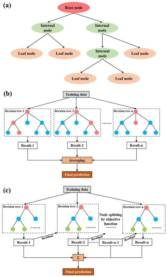
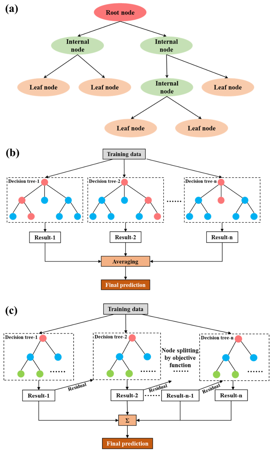
Based on their underlying learning mechanisms, the five algorithms can be divided into two categories: tree-based models (DT, RF, and XGBoost) and distance- or margin-based models (KNN and SVR). The principles of the three tree-based models are illustrated in Figure 3.

Figure 3. Schematic illustration of the three tree-based models: (a) Decision Tree; (b) Random Forest; (c) XGBoost.

(1)

Decision tree:

Decision Tree is a non-parametric regression algorithm that recursively partitions the feature space to minimize the prediction error within each leaf node. The objective function is

$$\underset{T}{min} {\displaystyle {\sum }_{m=1}^M} {\sum }_{x_i\in R_m} (y_i-{\overline{y}}_{R_m}{)}^2$$

(2)

where T denotes the tree structure, M is the number of leaf nodes, $y_i$ is the target value of the i-th training sample, and ${\overline{y}}_{R_m}$ is the mean target value of samples in the m-th leaf node. For each candidate split, the loss function is calculated as:

$$\mathrm{L}\mathrm{o}\mathrm{s}\mathrm{s}(j,s)={\sum }_{x_i\in R_1(j,s)} (y_i-\overline{y}{R}_1{)}^2+\sum x_i\in R_2(j,s)(y_i-{\overline{y}}_{R_2}{)}^2$$

(3)

where j and s denote the splitting feature and threshold, respectively. During training, the optimal split is selected by minimizing the loss function recursively until predefined stopping criteria, such as the maximum tree depth or the minimum number of samples in a leaf node, are satisfied.

(2)

Random forest

Random Forest is an ensemble learning algorithm consisting of multiple Decision Trees. The final prediction is obtained by averaging the outputs of all trees:

$$\widehat{y}={\displaystyle \frac{1}{T}}{\displaystyle {\sum }_{t=1}^T} h_t(x)$$

(4)

where $\widehat{y}$ is the predicted value, $T$ is the number of trees, and $h_t(x)$ represents the prediction of the t-th tree.

The mean squared error (MSE), used as the splitting criterion during training, is defined as

$$\mathrm{MSE}={\displaystyle \frac{1}{N}}{\displaystyle {\sum }_{i=1}^N} (y_i-{\widehat{y}}_i{)}^2$$

(5)

where N is the number of samples. As illustrated in Figure 3b, bootstrap sampling is first applied to generate multiple subsets from the original CFD dataset. Each Decision Tree is then trained independently using different sample and feature subsets. The final prediction is obtained by averaging the outputs of all trees, thereby improving prediction accuracy and reducing overfitting.

(3)

XGBoost

XGBoost is an efficient gradient boosting algorithm that iteratively constructs an ensemble of Decision Trees. Its objective function is expressed as

$$L^{(t)}={\displaystyle {\sum }_{i=1}^n} l\left(y_i,{\widehat{y}}_i^{(t-1)}+f_t(x_i)\right)+\mathsf{\Omega }(f_t)$$

(6)

where the objective consists of a training loss term and a regularization term. To improve computational efficiency, the objective function is approximated using a second-order Taylor expansion:

$$L^{(t)}\approx {\displaystyle {\sum }_{i=1}^n} \left[g_i{f}_t\left(x_i\right)+{\displaystyle \frac{1}{2}}{h}_i{f}_t(x_i{)}^2\right]+\mathsf{\Omega }\left(f_t\right)$$

(7)

where $g_i$ and $h_i$ are the first- and second-order derivatives of the loss function, respectively. The regularization term is defined as

$$\mathsf{\Omega }\left(f\right)=\gamma M+{\displaystyle \frac{1}{2}}\lambda {\displaystyle {\sum }_{j=1}^M} {\omega }_j^2$$

(8)

where $M$ is the number of leaf nodes, ${\omega }_j$ is the weight of the j-th leaf node, and $\gamma$ and $\lambda$ are regularization parameters controlling model complexity. By incorporating the regularization term, XGBoost effectively improves model generalization and mitigates overfitting.

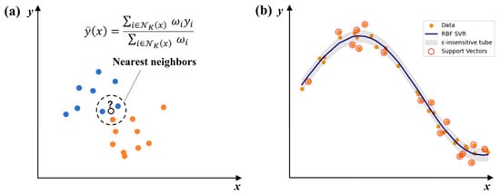
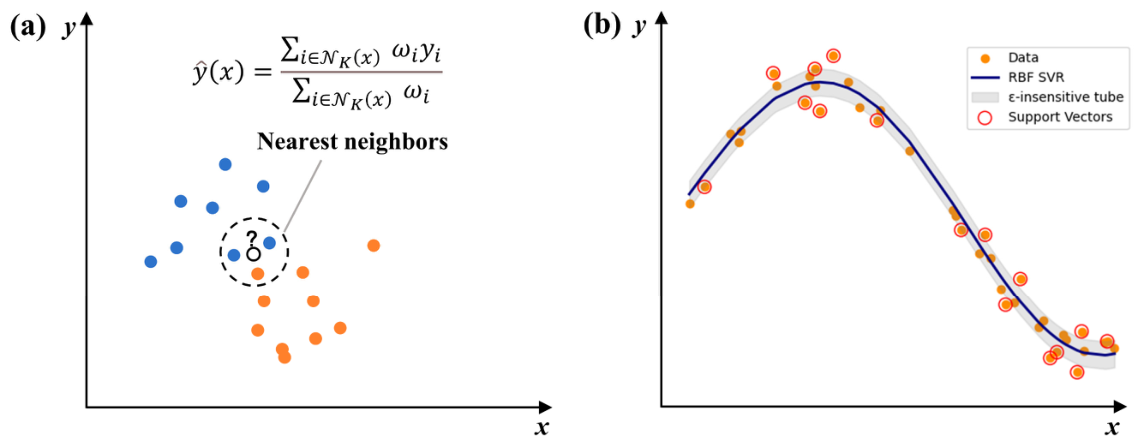
The principles of the two distance- and margin-based regression models are illustrated in Figure 4.

Figure 4. Schematic illustration of the two distance- and margin-based regression models: (a) K-Nearest Neighbors (KNN); (b) Support Vector Regression (SVR).

(1)

KNN

K-Nearest Neighbors (KNN) is a non-parametric regression algorithm that predicts the target value based on the responses of the nearest neighboring samples. The Euclidean distance between a query sample and each training sample is calculated as

$$d\left(x,x_i\right)=\sqrt{{\displaystyle {\sum }_{j=1}^n} (x_j-x_{ij}{)}^2}$$

(9)

where x is the feature vector of the query sample, $x_i$ is the feature vector of the i-th training sample, and n is the number of input features. The prediction is then obtained as the weighted average of the target values of the K nearest neighbors:

$$\widehat{y}(x)={\displaystyle \frac{\sum _{i\in {\mathcal{N}}_K(x)} {\omega }_i{y}_i}{\sum _{i\in {\mathcal{N}}_K(x)} {\omega }_i}}$$

(10)

where the weight assigned to each neighbor is inversely proportional to its distance from the query sample,

$${\omega }_i={\displaystyle \frac{1}{d(x,x_i)+\epsilon }}$$

(11)

and $\epsilon$ is a small positive constant introduced to avoid division by zero.

(2)

SVR

Support Vector Regression (SVR) constructs an optimal regression function in a high-dimensional feature space through nonlinear kernel mapping. Its optimization objective is

$$\underset{w,b,{\xi }_i,{\xi }_i^{*}}{min} {\displaystyle \frac{1}{2}}\parallel w{\parallel }^2+C{\displaystyle {\sum }_{i=1}^n} ({\xi }_i+{\xi }_i^{*})$$

(12)

$$\left\{\begin{array}{c}{y}_i-w^T{x}_i-b\le \epsilon +{\xi }_i\\ w^T{x}_i+b-y_i\le \epsilon +{\xi }_i^{*}\\ {\xi }_i,{\xi }_i^{*}\ge 0\end{array}\right.$$

(13)

where $w$ is the weight vector, b is the bias term, C is the penalty parameter, $\epsilon$ defines the width of the insensitive loss region, and ${\xi }_i$ and ${\xi }_i^{*}$ are slack variables that allow prediction errors exceeding the $\epsilon$-insensitive region. This formulation enables SVR to achieve good generalization while maintaining robustness to noise.

Before model training, the hyperparameters of all machine learning algorithms were determined. The detailed parameter settings for each model are summarized in Table 3. To ensure the reproducibility of the experiments, the random seed was fixed at RANDOM_SEED = 40. In addition, multithreaded parallel computing was enabled for Random Forest (RF), Extreme Gradient Boosting (XGBoost), Decision Tree (DT), and K-Nearest Neighbors (KNN) to accelerate the training process.

Table 3. Hyperparameter settings of the machine learning models used in this study.

Model	Hyperparameter	Setting
Decision Tree (DT)	Maximum tree depth (max_depth)	13
	Minimum number of samples required for a leaf node (min_samples_leaf)	3
	Minimum number of samples required for an internal node split (min_samples_split)	2
	Number of features considered for splitting (max_features)	sqrt
	Split criterion (criterion)	Squared error
Random Forest (RF)	Number of decision trees (n_estimators)	1000
	Maximum tree depth (max_depth)	30
	Minimum number of samples required for a leaf node (min_samples_leaf)	1
	Minimum number of samples required for an internal node split (min_samples_split)	2
	Number of features considered for splitting (max_features)	sqrt (default)
Extreme Gradient Boosting (XGBoost)	Number of boosting trees (n_estimators)	300
	Learning rate (learning_rate)	0.05
	Maximum tree depth (max_depth)	13
	Minimum child weight (min_child_weight)	0.5
	Subsample ratio (subsample)	0.9
	Column sampling ratio (colsample_bytree)	0.9
	Minimum loss reduction (gamma)	0 (default)
	L1 regularization coefficient (reg_alpha)	0 (default)
	L2 regularization coefficient (reg_lambda)	1 (default)
K-Nearest Neighbors (KNN)	Number of neighbors (n_neighbors)	15
	Weighting strategy (weights)	Distance-based
	Distance metric (metric)	Manhattan distance
	Minkowski distance parameter (p)	1
Support Vector Regression (SVR)	Kernel function (kernel)	Radial basis function (RBF)
	Penalty parameter (C)	1.0
	Epsilon-insensitive loss parameter (epsilon)	0.1

2.4. Model Training and Performance Evaluation

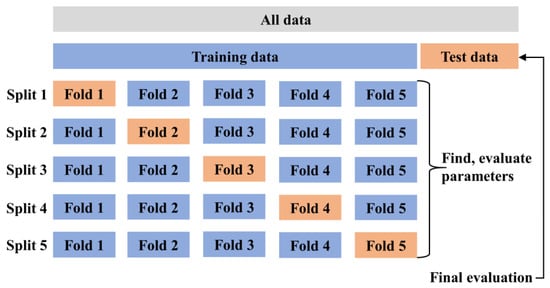
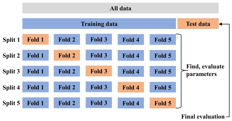
The datasets were randomly divided into training and testing sets using an 80:20 ratio. To improve model robustness and reduce the risk of overfitting, five-fold cross-validation was employed during model training. As illustrated in Figure 5, the dataset was partitioned into five equally sized subsets. In each iteration, one subset was used as the validation set, while the remaining four subsets were used for training. This process was repeated five times so that each subset served as the validation set once. The final model performance was obtained by averaging the results over the five validation runs.

Figure 5. Schematic illustration of the five-fold cross-validation procedure.

The predictive performance of the five ML algorithms was evaluated using the coefficient of determination ($R^2$), mean absolute error (MAE), and root mean square error (RMSE), defined as follows, while the standard deviation and 95% confidence interval of each metric were calculated from five-fold cross-validation results to quantify the uncertainty in model performance.

$$R^2=1-{\displaystyle \frac{{\displaystyle {\sum }_{i=1}^n} (y_i-\widehat{y}i{)}^2}{\sum {i=1}^n(y_i-\overline{y}{)}^2}}$$

(14)

$$MAE={\displaystyle \frac{1}{n}}{\displaystyle {\sum }_{i=1}^n} |{\widehat{y}}_i-y_i|$$

(15)

$$RMSE=\sqrt{{\displaystyle \frac{1}{n}}{\displaystyle {\sum }_{i=1}^n} ({\widehat{y}}_i-y_i{)}^2}$$

(16)

where $y_i$ and $\widehat{y}i$ denote the actual and predicted values of the i-th sample, respectively, and $\overline{y}$ is the mean of the observed values. A higher $R^2$ and lower MAE and RMSE indicate better predictive performance.

3. Results and Discussion

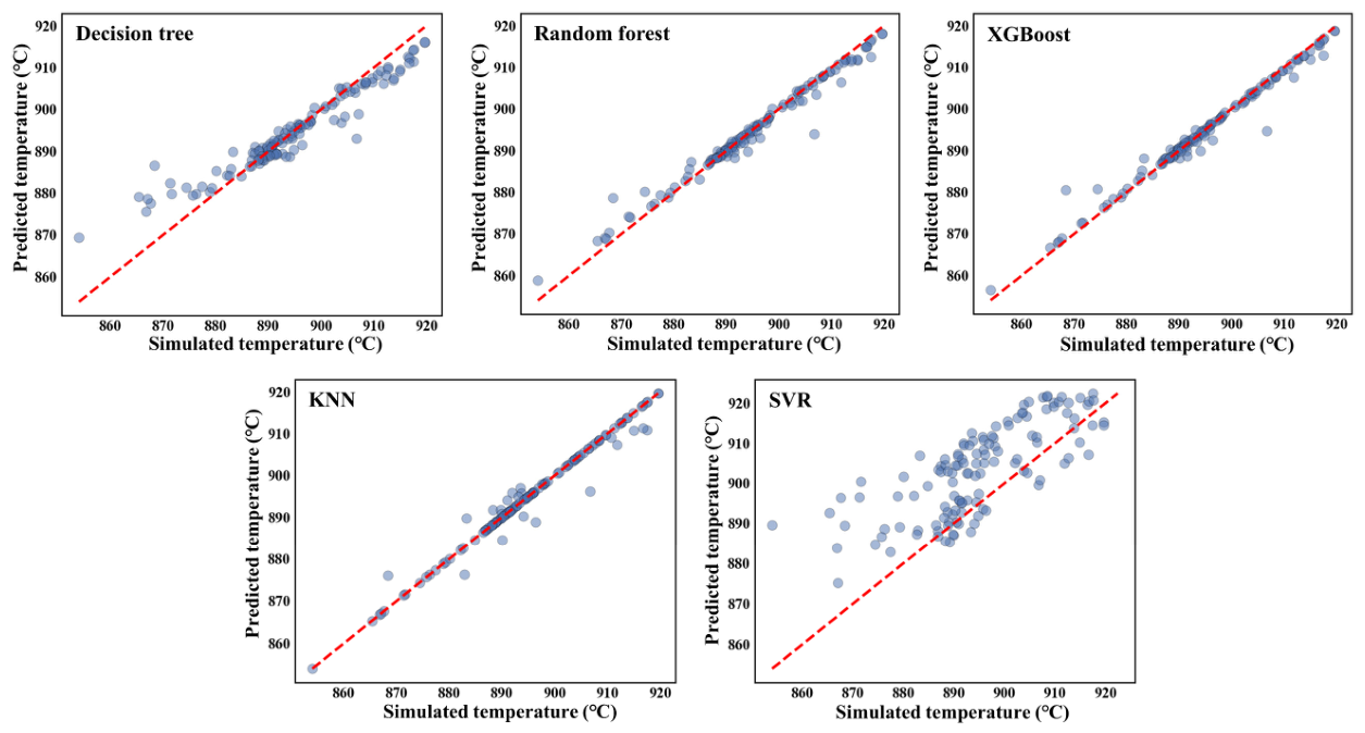
Figure 6 compares the average cross-sectional temperatures predicted by the five machine learning models with the corresponding CFD simulation results. Among the evaluated models, SVR shows the largest deviation from the CFD results, indicating the lowest prediction accuracy. In contrast, Random Forest and XGBoost exhibit much closer agreement with the CFD simulations than Decision Tree and KNN, with most predictions clustered near the identity line. These results suggest that ensemble tree-based models are more effective in capturing the nonlinear relationships between the input physical variables and the thermal field, leading to improved prediction accuracy.

Figure 6. Parity plots of the cross-sectional average temperatures predicted by the five ML models against the CFD simulation results.

To quantitatively evaluate the overall predictive performance of the five machine learning (ML) models, Table 4 summarizes the mean, standard deviation, and 95% confidence interval of the coefficient of determination ($R^2$), mean absolute error (MAE), and root mean square error (RMSE) calculated over the entire dataset. Overall, except for the support vector regression (SVR) model, all models achieved ($R^2$) values exceeding 0.95, with the Random Forest and XGBoost models exhibiting the best predictive performance. However, owing to the non-uniform temperature distribution within the aluminum reduction cell, particularly the large temperature gradients near the solidification interface that play a decisive role in the formation of the side ledge, the overall evaluation metrics alone cannot fully reflect model performance in this critical region. Therefore, a dedicated error analysis was further conducted for the region corresponding to the side ledge profile, and the results are presented in Table 5. This region exhibits the steepest temperature gradients, directly determining the morphology of the side ledge and thus requiring higher prediction accuracy. As shown in Table 5, even in this thermally challenging region, the Random Forest and XGBoost models maintained high predictive accuracy, achieving ($R^2$) values of 0.945 and 0.944, respectively. Moreover, their MAE and RMSE values were substantially lower than those of the Decision Tree, K-Nearest Neighbors (KNN), and SVR models. These results demonstrate that the two ensemble learning models retain reliable predictive capability in the region most closely associated with side ledge formation, making them well suited for predicting the side ledge morphology in aluminum reduction cells. Combining the results presented in Figure 6 and Table 4 and Table 5, it can be concluded that the Random Forest and XGBoost models achieve superior predictive accuracy for cross-sectional temperature prediction in the molten region of the aluminum reduction cell.

Table 4. Prediction performance of the five ML models for cross-sectional average temperature.

Model	R2	MAE	RMSE
Decision Tree	0.9674 ± 0.0046 (0.9577, 0.9756)	8.6644 ± 0.6679 (7.4434, 10.0129)	23.4440 ± 1.7366 (20.1555, 26.8912)
Random Forest	0.9852 ± 0.0033 (0.9777, 0.9906)	5.4644 ± 0.5980 (4.3529, 6.6614)	15.8281 ± 1.7134 (12.6092, 19.2197)
XGBoost	0.9843 ± 0.0030 (0.9777, 0.9896)	5.9602 ± 0.5986 (4.8488, 7.1556)	16.2850 ± 1.5893 (13.1655, 19.3936)
KNN	0.9584 ± 0.0063 (0.9454, 0.9699)	9.2269 ± 0.7595 (7.8140, 10.6760)	26.5037 ± 2.0318 (22.5240, 30.3320)
SVM	0.7163 ± 0.0066 (0.7029, 0.7285)	29.4511 ± 1.1976 (27.0428, 31.7780)	69.2036 ± 1.5606 (65.9581, 72.1658)

Note: Values are presented as mean ± standard deviation (std), with 95% confidence interval in parentheses.

Table 5. Prediction accuracy of different ML models in the trough profile region.

Model	R2	MAE	RMSE
Decision Tree	0.8775 ± 0.0176 (0.8397, 0.9088)	7.3918 ± 0.5859 (6.3409, 8.6251)	22.1270 ± 1.7079 (18.8722, 25.5699)
Random Forest	0.9452 ± 0.0132 (0.9157, 0.9670)	4.4714 ± 0.5486 (3.4738, 5.5993)	14.8048 ± 1.8082 (11.3559, 18.4571)
XGBoost	0.9440 ± 0.0121 (0.9167, 0.9648)	4.8887 ± 0.5421 (3.9018, 6.0177)	14.9641 ± 1.6816 (11.6877, 18.2614)
KNN	0.8528 ± 0.0239 (0.8022, 0.8972)	7.3438 ± 0.6680 (6.1041, 8.6481)	24.2575 ± 2.1025 (20.0923, 28.1749)
SVM	0.5899 ± 0.0247 (0.5385, 0.6361)	18.5438 ± 0.9862 (16.6366, 20.4202)	40.4940 ± 1.7040 (37.0444, 43.7336)

Note: Values are presented as mean ± standard deviation (std), with 95% confidence interval in parentheses.

Based on the optimized hyperparameter settings described above, the superior performance of the Random Forest (RF) model can be attributed primarily to its ability to capture the nonlinear and strongly coupled characteristics of the thermal-MHD system. The nodal temperature is jointly influenced by the local Joule heat, effective thermal conductivity (ETC), and the three velocity components, which represent heat generation, heat conduction, and convective heat transfer, respectively. These physical variables interact in a highly nonlinear manner rather than contributing independently. For example, the temperature response associated with a given level of Joule heat may vary considerably under different local thermal conductivity and flow conditions.

The RF model is particularly well suited to learning such complex relationships because its tree-based ensemble structure partitions the feature space into multiple local regions, enabling it to capture nonlinear responses, threshold effects, and high-order feature interactions without requiring an explicit mathematical formulation. Furthermore, ensemble averaging over multiple decision trees effectively reduces sensitivity to local fluctuations and data noise, thereby improving the robustness and generalization capability of the model for the spatially heterogeneous nodal dataset considered in this study. The large number of node-level samples also provides sufficient coverage of diverse local thermal and flow states, allowing the RF model to achieve an effective balance between predictive accuracy and generalization performance.

Although the proposed RF model is purely data-driven and does not explicitly solve the governing equations of the thermal-MHD system, the predicted temperature fields remain physically consistent with the CFD benchmark. The reconstructed temperature distributions successfully preserve the major spatial characteristics of the CFD results, including the locations of high- and low-temperature regions as well as the temperature variations near the solidification interface. Consequently, the reconstructed side ledge profiles agree closely with those obtained from the CFD simulations without introducing noticeable nonphysical oscillations or distortions. These results demonstrate that the proposed RF surrogate model effectively preserves the dominant physical characteristics of the thermal-MHD system within the investigated operating conditions while significantly reducing the computational cost of temperature field prediction.

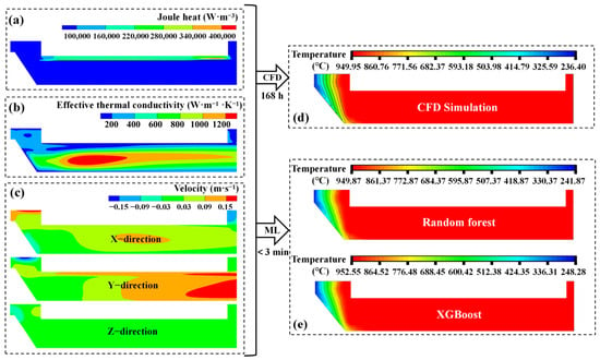
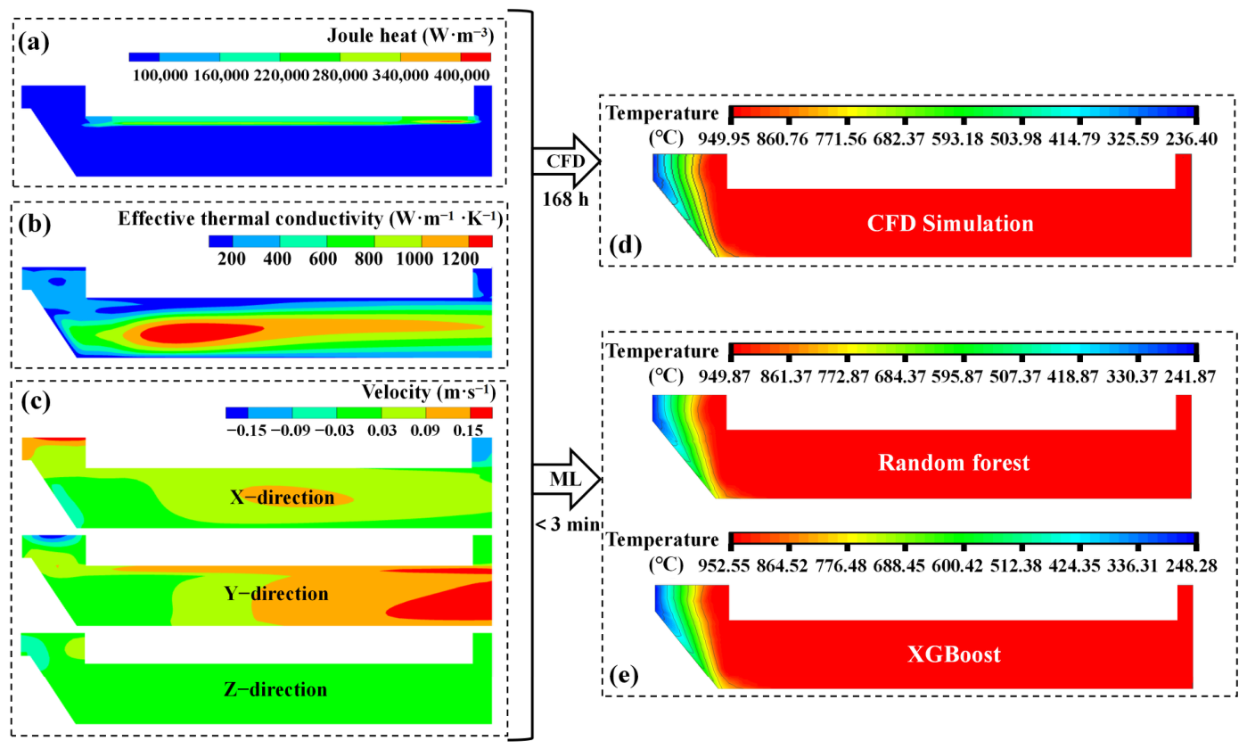
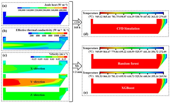
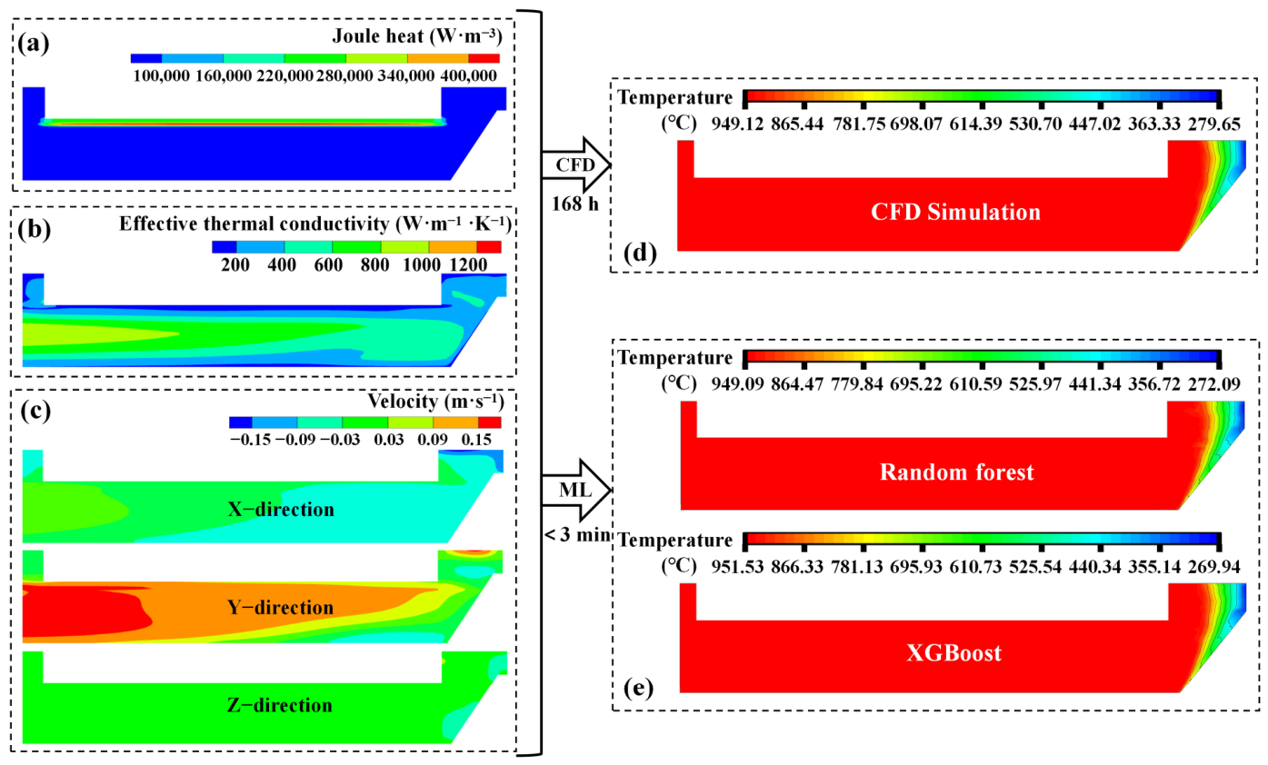
To further compare the predictive performance of the two best-performing models, Figure 7 and Figure 8 present the input feature distributions before side ledge solidification, including Joule heating, effective thermal conductivity (ETC), and the three velocity components, together with the corresponding temperature fields after side ledge solidification predicted by Random Forest, XGBoost, and the CFD simulations. The results are shown for the x = 8.54 m cross-section on both Sides A and B of the aluminum reduction cell. Despite the different input feature distributions, both models accurately reproduced the CFD-predicted temperature fields. Once trained, the models generated the corresponding temperature fields within approximately 3 min, demonstrating their potential for rapid prediction of cross-sectional thermal fields after side ledge solidification. Although both models achieved high prediction accuracy, Random Forest more accurately captured the temperature extremes. For the representative cross-section shown in Figure 7, the maximum and minimum temperatures predicted by Random Forest were 949.87 °C and 241.87 °C, differing from the CFD results by only 0.08 °C and 5.47 °C, respectively. The corresponding deviations for XGBoost were 2.60 °C and 11.88 °C.

Figure 7. Input feature distributions and predicted temperature fields at the x = 8.54 m cross-section in the molten bath on Side A of the aluminum reduction cell: (a) Joule heating distribution; (b) effective thermal conductivity distribution; (c) three-dimensional velocity distribution; (d) temperature field after side ledge solidification obtained from the CFD simulation; (e) temperature field after side ledge solidification predicted by the ML model.

Figure 8. Input feature distributions and predicted temperature fields at the x = 8.54 m cross-section in the molten bath on Side B of the aluminum reduction cell: (a) Joule heating distribution; (b) effective thermal conductivity distribution; (c) distributions of the three velocity components; (d) temperature field after side ledge solidification obtained from the CFD simulation; (e) temperature field after side ledge solidification predicted by the ML model.

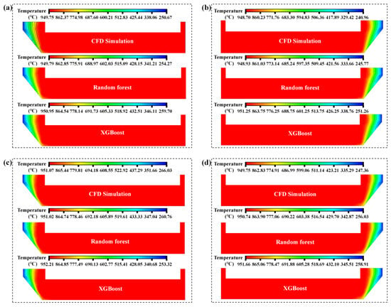
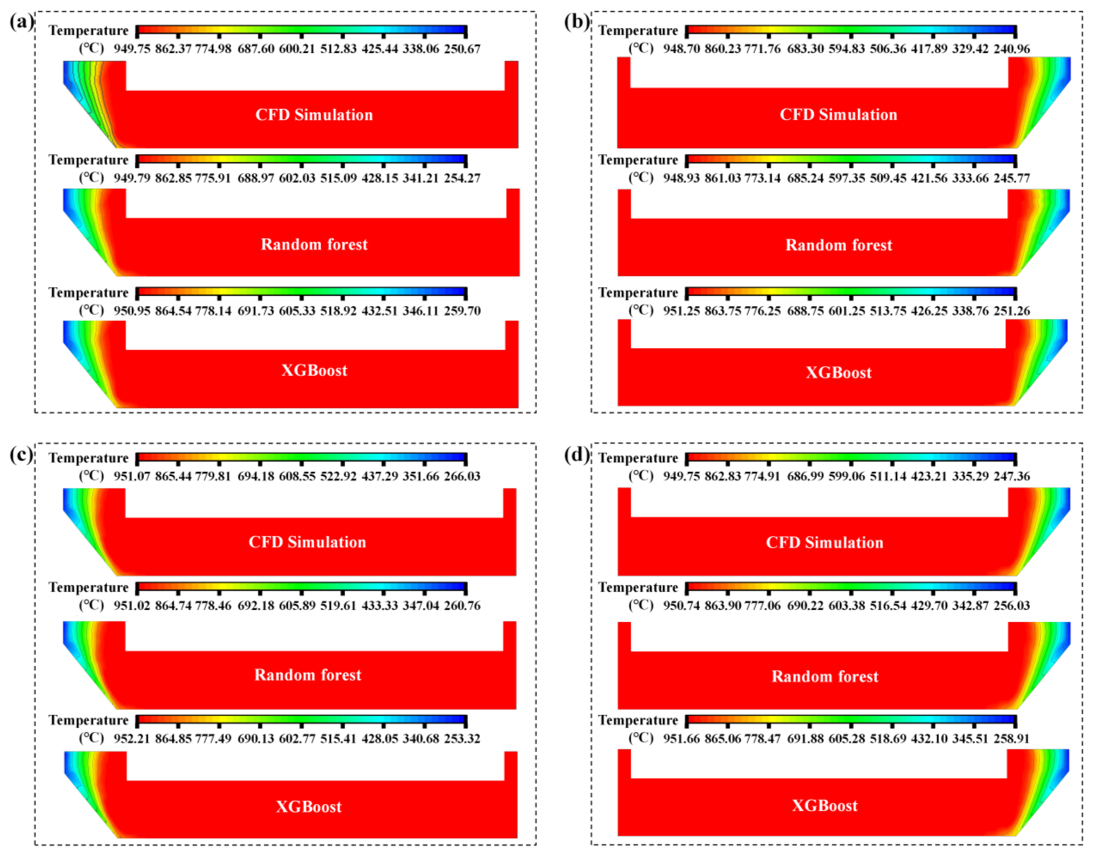
Additional validation was performed on two cross-sections near the ends of the aluminum reduction cell (x = 2.24 m and x = 15.375 m), as shown in Figure 9. For both Sides A and B, the temperature fields predicted by the two models remained in close agreement with the CFD results, confirming the robustness of the proposed ML-based prediction framework. Nevertheless, Random Forest consistently yielded smaller deviations in both the maximum and minimum temperatures, with errors not exceeding 0.23 °C and 8.67 °C, respectively. These results indicate that, while both models provide reliable thermal field reconstruction, Random Forest offers superior accuracy for predicting the extreme temperatures that govern side ledge formation.

Figure 9. Comparison of the temperature fields predicted by the CFD simulation and the ML model at cross-sections near the ends of the molten bath: (a) Side A, x = 2.24 m; (b) Side B, x = 2.24 m; (c) Side A, x = 15.375 m; (d) Side B, x = 15.375 m.

Based on a comprehensive comparison of the five machine learning models in terms of R², MAE, RMSE, cross-sectional average temperature, and temperature distribution fields, the Random Forest model exhibits the highest overall prediction accuracy. This model enables fast and accurate reconstruction of the post-solidification temperature field of the side ledge using the pre-solidification distributions of Joule heating, effective thermal conductivity, and flow velocity on each cross-section. In addition, its prediction time is significantly shorter than that of the CFD simulations, demonstrating its strong potential for efficient thermal field evaluation in aluminum reduction cells.

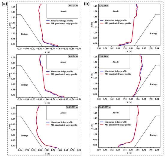
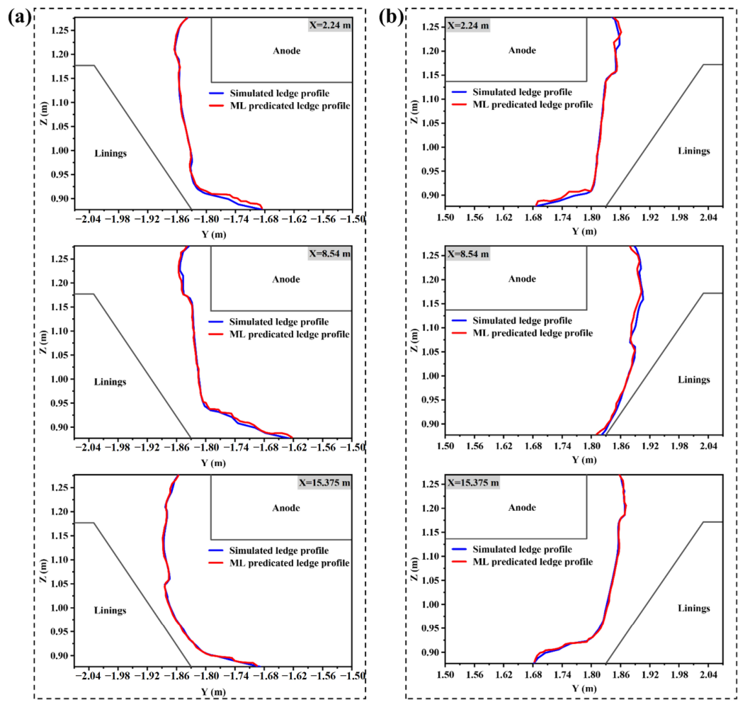
Based on the electrolyte solidus temperature, the side ledge profiles predicted by the Random Forest model were extracted from the temperature fields shown in Figure 7, Figure 8 and Figure 9 and compared with the corresponding CFD results. The comparison, presented in Figure 10, shows excellent agreement between the predicted and simulated side ledge profiles at all six locations across the three cross-sections, with an average thickness deviation of only 0.0153 m. These results demonstrate that the Random Forest model can accurately reconstruct side ledge morphology from the predicted temperature fields.

Figure 10. Comparison of the side ledge profiles predicted by the Random Forest model and the CFD simulations: (a) Side A; (b) Side B.

Conventional forward prediction of side ledge formation in aluminum reduction cells is generally performed using iterative electro–thermal coupled slice models. To reduce computational cost, reduced-order approaches have been proposed to transform three-dimensional slice models into two-dimensional representations, thereby accelerating the simulation process. Although these methods significantly improve computational efficiency, they typically assume a uniform effective thermal conductivity in the molten bath, which limits their ability to rapidly predict side ledge profiles at different locations within the cell. In contrast, the proposed framework first performs an MHD simulation for the pre-solidification state and then predicts side ledge profiles using the spatial distributions of the MHD variables extracted from individual two-dimensional cross-sections. By preserving the spatial variations in the coupled MHD fields throughout the molten bath, the proposed method provides a more faithful representation of local thermal conditions while enabling rapid prediction of side ledge morphology across the entire aluminum reduction cell. This combination of accuracy and computational efficiency makes the proposed framework well suited for engineering applications requiring fast, spatially resolved thermal field analysis.

It should be noted that the region near the solid–liquid interface, where the temperature gradient is relatively large, represents a critical area for evaluating the predictive capability of the proposed model. Comparison between the machine learning predictions and CFD results shows that the model can effectively reproduce the temperature variation trends and isotherm distributions near the solid–liquid interface. Although small prediction deviations exist in regions with rapid temperature variation near the interface, no obvious systematic bias was observed. The predicted side ledge profile and overall thermal field characteristics remain consistent with the CFD results. This indicates that the selected input features can effectively characterize the local heat transfer state near the interface and provide reliable predictions in this critical region. Therefore, although the proposed machine learning model is a data-driven approach and does not explicitly solve the coupled thermal–MHD governing equations, it can preserve the dominant physical characteristics reflected by the CFD simulations and satisfy the requirements for rapid side ledge prediction under the operating condition investigated in this study.

From an application perspective, the proposed framework adopts an offline–online strategy. Although CFD/MHD simulations require considerable computational resources, they are performed offline to generate the training database. Once the surrogate model has been trained, it can rapidly reconstruct the temperature field and side ledge profile of previously unseen cross-sections under the same operating condition without repeating the CFD simulations. Therefore, the offline computational cost does not affect the online reconstruction efficiency. In future practical applications, CFD/MHD simulations corresponding to representative operating conditions can be performed in advance to establish a comprehensive multi-condition database. A surrogate model trained using such a database could then be used to estimate the temperature field and side ledge state based on real-time operating parameters acquired from the aluminum reduction cell. This framework provides potential support for digital twin applications, real-time process monitoring, and operational decision-making for aluminum reduction cells.

4. Conclusions

This study develops a CFD-driven machine learning surrogate model for rapid prediction of cross-sectional temperature fields and side ledge morphology in an aluminum reduction cell under magnetohydrodynamic (MHD) coupling conditions. A high-fidelity dataset is generated from MHD-CFD simulations, and five machine learning models are systematically evaluated and compared.

(1)

Key physical variables, including heat generation, effective thermal transport properties, and velocity components in three directions, are extracted from multiple cross-sections prior to side ledge formation. These variables form a high-fidelity dataset for model training and evaluation. Based on this dataset, the predictive performance of Decision Tree, Random Forest, XGBoost, K-Nearest Neighbors (KNN), and Support Vector Regression (SVR) models is systematically assessed. The results show that Random Forest achieves the best overall performance, followed by XGBoost, Decision Tree, KNN, and SVR.

(2)

The Random Forest model provides the most accurate predictions of both temperature fields and side ledge morphology. The predicted temperature distributions agree well with CFD results, with maximum deviations of 0.23 °C and 8.67 °C for peak and minimum temperatures, respectively. The average error in side ledge thickness is 0.0153 m, demonstrating that the model can reliably reproduce local thermal behavior and geometry.

(3)

Compared with conventional CFD simulations, the Random Forest surrogate model reduces computation time from approximately 168 h to 3 min while maintaining high accuracy. By capturing spatial variations across different cross-sections, the proposed method enables fast prediction of temperature fields and side ledge profiles throughout the cell. This provides an efficient tool for thermal state evaluation, process optimization, and digital twin development of aluminum reduction cells.

References

- Reny, P.; Segatz, M.; Haakonsen, H.; Gikling, H.; Assadian, M.; Høines, J.F.; Kvilhaug, E.; Bardal, A.; Solbu, E. Hydro’s new karmøy technology pilot: Start-up and early operation. In Light Metals 2021; Perander, L., Ed.; TMS: Pittsburgh, PA, USA, 2021; pp. 608–617. [Google Scholar]
- Dupuis, M. Thermo-electric design of a 400 kA cell using mathematical models: A tutorial. In Light Metals 2000; Peterson, R.D., Ed.; TMS: Nashville, TN, USA, 2000; pp. 297–302. [Google Scholar]
- Langlois, S.; Rappaz, J.; Martin, O.; Caratini, Y.; Flueck, M.; Masserey, A.; Steiner, G. 3D coupled MHD and thermo-electrical modelling applied to AP technology pots. In Light Metals 2015; Hyland, M., Ed.; TMS: Orlando, FL, USA, 2015; pp. 769–775. [Google Scholar]
- Zhu, J.; Li, J. Transient Simulation of Bath Temperature inside Aluminum Reduction Cells. Metals 2020, 10, 379. [Google Scholar] [CrossRef] [Scilit]
- Sanogo, B.; Dion, L.; Gaboury, S.; Kiss, L.; Roger, T.; Guérard, S.; Bilodeau, J.F. A Review of Challenges and Solutions in Ledge Control and Measurement in Aluminium Electrolysis Cell. In Light Metals 2024; Wagstaff, S., Ed.; Springer: Cham, Switzerland, 2024; pp. 577–585. [Google Scholar]
- Dupuis, M.; Bojarevics, V. Weakly coupled thermo-electric and MHD mathematical models of an aluminium electrolysis cell. In Light Metals 2005; Kvande, H., Ed.; TMS: San Francisco, CA, USA, 2005; pp. 449–454. [Google Scholar]
- Hua, J.S.; Rudshaug, M.; Droste, C.; Jorgensen, R.; Giskeodegard, N.-H. Numerical simulation of multiphase magnetohydrodynamic flow and deformation of electrolyte-metal interface in aluminum electrolysis cells. Metall. Mater. Trans. B 2018, 49, 1246–1266. [Google Scholar] [CrossRef] [Scilit]
- Dupuis, M. Computation of Aluminum Reduction Cell Energy Balance Using ANSYS® Finite Element Models. In Light Metals 1998; Welch, B., Ed.; TMS: Warrendale, PA, USA, 1998; pp. 409–417. [Google Scholar]
- Lu, D.X.; Mao, J.H.; Ban, Y.G.; Qi, X.Q.; Yang, Q.C.; Dong, H. Development of NEUI500kA family high energy efficiency aluminum reduction pot (HEEP) technology. In Light Metals 2011; Lindsay, J., Ed.; TMS: San Diego, CA, USA, 2011; pp. 455–460. [Google Scholar]
- Cui, X.F.; Zhou, Y.W.; Yang, J.H. An improved finite element model for thermal balance analysis of Aluminum electrolysis cells. In Light Metals 2014; Grandfield, J., Ed.; TMS: San Diego, CA, USA, 2014; pp. 661–666. [Google Scholar]
- Romerio, M.V.; Flueck, M.; Rappaz, J.; Safa, Y. Determination and influence of the ledge shape on electrical potential and fluid motions in a smelter. In Light Metals 2005; Kvande, H., Ed.; TMS: San Francisco, CA, USA, 2005; pp. 461–468. [Google Scholar]
- Safa, Y.; Flueck, M.; Rappaz, J. Numerical simulation of thermal problems coupled with magnetohydrodynamic effects in aluminium cell. Appl. Math. Model. 2009, 33, 1479–1492. [Google Scholar] [CrossRef] [Scilit]
- Pianykh, A.A.; Arkhipov, G.V.; Tretyakov, Y.A. Mathematical model of magnetic hydrodynamics and heat transfer in an aluminum reduction cell. Russ. J. Non-Ferr. Met. 2020, 61, 65–73. [Google Scholar] [CrossRef] [Scilit]
- Wang, Q.; Gosselin, L.; Fafard, M.; Peng, J.; Li, B. Numerical investigation on the impact of anode change on heat transfer and fluid flow in aluminum smelting cells. Metall. Mater. Trans. B 2016, 47, 1228–1236. [Google Scholar]
- Zhou, S.; Diop, M.A.; Gao, B.L.; Wang, Z. Controlled ledge profile of aluminum smelting cell using sidewalls heat exchangers supplied with molten salt. J. Sustain. Metall. 2023, 9, 550–563. [Google Scholar] [CrossRef] [Scilit]
- Zhang, H.L.; Ran, L.; Zou, Z.; He, G.; Tang, Y.; Li, J. Effect of current transient enhancement on thermal field of aluminum electrolysis cell for the accommodation of wind power. J. Sustain. Metall. 2018, 4, 359–366. [Google Scholar] [CrossRef] [Scilit]
- Severo, D.S.; Schneider, A.F.; Pinto, E.C.V.; Gusberti, V.; Potocnik, V. Modeling magnetohydrodynamics of aluminum electrolysis cells with ANSYS and CFX. In Light Metals 2005; Kvande, H., Ed.; TMS: San Francisco, CA, USA, 2005; pp. 475–480. [Google Scholar]
- Ran, L.; Li, J.; Zou, Z.; Zhang, B.; Li, Q.; Yang, S.; Zhang, H. Interaction investigation between ledge evolution and magnetohydrodynamic flow under normal and enhanced current conditions in aluminum reduction cell. Metall. Mater. Trans. B 2025, 56, 2748–2767. [Google Scholar] [CrossRef] [Scilit]
- Aly, A.M. Machine Learning Reshaping Computational Fluid Dynamics: A Paradigm Shift in Accuracy and Speed. Fluids 2025, 10, 275. [Google Scholar] [CrossRef] [Scilit]
- Mao, R.; Lan, Y.; Liang, L.; Yu, T.; Mu, M.; Leng, W.; Long, Z. Rapid CFD Prediction Based on Machine Learning Surrogate Model in Built Environment: A Review. Fluids 2025, 10, 193. [Google Scholar] [CrossRef] [Scilit]
- Li, X.; Sun, W.; Qin, C.; Yan, Y.; Zhang, L.; Tu, J. Evaluation of supervised machine learning regression models for CFD-based surrogate modelling in indoor airflow field reconstruction. Build. Environ. 2025, 267, 112173. [Google Scholar] [CrossRef] [Scilit]
- Stevanović, S.; Dashti, H.; Milošević, M.; Al-Yakoob, S.; Stevanović, D. Comparison of ANN and XGBoost surrogate models trained on small numbers of building energy simulations. PLoS ONE 2024, 19, e0312573. [Google Scholar] [CrossRef]
- Liu, Y.R.; Zhang, H.M.; Shen, Y.S. A data-driven approach for the quick prediction of in-furnace phenomena of pulverized coal combustion in an ironmaking blast furnace. Chem. Eng. Sci. 2022, 260, 117945. [Google Scholar] [CrossRef] [Scilit]
- Lu, T.T.; Li, K.; Zhao, H.L.; Wang, W.; Zhou, Z.; Cai, X.; Liu, F. Rapid prediction of flow and concentration fields in solid-liquid suspensions of slurry electrolysis tanks. Int. J. Miner. Metall. Mater. 2024, 31, 2006–2016. [Google Scholar] [CrossRef] [Scilit]
- Li, J.L.; Zhu, R.J.; Zhou, P.; Song, Y.-P.; Zhou, C.Q. Prediction of the cohesive zone in a blast furnace by integrating CFD and SVM modelling. Ironmak. Steelmak. 2021, 48, 284–291. [Google Scholar] [CrossRef] [Scilit]
Disclaimer/Publisher’s Note: The statements, opinions and data contained in all publications are solely those of the individual author(s) and contributor(s) and not of MDPI and/or the editor(s). MDPI and/or the editor(s) disclaim responsibility for any injury to people or property resulting from any ideas, methods, instructions or products referred to in the content. |
© 2026 by the authors. Licensee MDPI, Basel, Switzerland. This article is an open access article distributed under the terms and conditions of the Creative Commons Attribution (CC BY) license.