


Abstract
Large slewing bearings for wind turbines require sufficient hardening depth due to high contact stresses and cyclic loads. In this study, we combined electromagnetic–thermal–phase-transition coupled finite element analysis (FEA) with a surrogate model to predict the induction hardening depth of a dual-inductor system equipped with a magnetic flux concentrator. The air gap and the currents applied to the two inductors were used as input variables, and the hardening depth at five locations was calculated using FEA. Position 4 was identified as the critical location where the minimum hardening depth occurs. Since predictions based on limited FEA data may lead to overfitting and validation uncertainty, DNN, RSM, GPR, and SVR were compared, and LOOCV was applied to the comparison models. DNN predictions were adopted for the selection of candidate process conditions. When A1 and A2 were 8200 A and 8600 A, respectively, the predicted hardening depth was 6.17 mm. Under these conditions, additional FEA results showed a depth of 6.38 mm, while prototype measurements indicated 6.20 mm, representing a difference of 2.90%. This approach can be utilized to select candidate induction hardening conditions within the reviewed process range.
1. Introduction
Induction hardening is a common surface heat-treatment process widely used in various industries, such as the aerospace and automotive industries, to improve the mechanical properties of workpieces. This process selectively hardens the surface layer by rapidly heating a specific area of the workpiece using eddy currents generated by an alternating current applied to an inductor, followed by quenching. Because only the surface layer is heated and cooled rapidly, this process offers the advantages of minimal changes in the metallurgical properties of the internal structure and excellent process reproducibility. Furthermore, the formation of fine martensite and compressive residual stresses in the surface layer improves the fatigue life of mechanical components [1,2,3,4]. In particular, for components subjected to repeated rolling contact loading, such as slewing bearing raceways, the stress state in the surface and subsurface regions of the induction-hardened raceway is closely related to rolling contact fatigue life [5]. However, if the material is heated excessively or for an extended period, austenite grain growth may occur, which can reduce fatigue strength; therefore, precise process control is essential. As wind turbine systems increase in size, pitch and yaw slewing bearings are required to withstand higher contact stresses and cyclic loads. Therefore, for large components such as wind turbine slewing bearings, which can reach diameters of approximately 5000 mm, it is crucial to control process variables to ensure uniform heat-treatment quality while satisfying the required hardening depth and hardness. In the present study, a 4 MW-class pitch bearing was selected as a representative model to investigate the feasibility of the proposed FEA–DNN-based induction hardening depth prediction framework.
In the induction hardening process, the hardened depth, hardness, and microstructure are determined by various parameters, including the input current, heating and cooling times, coil geometry, workpiece geometry and material, and the air gap. Compressive residual stresses form in the hardened surface layer, resulting in a high fatigue life. The induction heat-treatment process involves a multiphysics problem in which electromagnetic, thermal, metallurgical phase transformations, and mechanical behavior are mutually coupled; however, the temperature dependence and nonlinearity of material properties make it difficult to quantitatively predict the process results. Numerical simulations based on finite element analysis are widely used as a method for analyzing such complex behavior.
Previous studies have extensively applied finite element analysis to induction heating and induction hardening processes. These studies have demonstrated that coupled electromagnetic–thermal–phase transformation analysis can effectively predict temperature history, hardening layer geometry, residual stresses, and microstructural changes under various process conditions [6,7,8,9,10].
Li et al. applied a magnetic flux concentrator to a mobile planar induction heating process and analyzed the surface temperature distribution and local heating characteristics as a function of process variables by comparing numerical simulation results with experimental data [11].
Recently, sensitivity analysis of process variables and data-driven modeling have been introduced to improve the efficiency of induction hardening process design. Studies utilizing experimental design, numerical simulation datasets, and machine learning have demonstrated the potential to predict hardness, hardening depth, stress changes, and temperature uniformity without performing iterative simulations or experiments for all process conditions [12,13,14,15,16].
However, previous studies have primarily focused on relatively simple geometries, small- to medium-sized components, or limited process conditions. The induction hardening process for large slewing bearings used in wind turbines is a non-steady-state transient process in which the raceway is gradually heated by a moving inductor, followed by phase transformation during the subsequent cooling process. Consequently, the hardening depth is influenced by a combination of various process variables, including long heating and cooling times, as well as factors such as air gap, inductor current, inductor position, and local geometric variations.
In addition, while high input energy is required to achieve the necessary hardening depth for large raceways, concentrating the current in a single inductor can cause localized overheating or melting. Therefore, a dual-inductor system incorporating a magnetic flux concentrator was employed to distribute the input energy and improve the uniformity of the heating zone. Evaluating all possible combinations of the current distribution acting on each inductor, the temperature distribution in the air gap, and the hardening depth as the inductors move, such as along the raceways of wind turbine slewing bearings using only iterative transient finite element analysis (FEA), would entail significant computational costs. Therefore, we sought to construct a DNN surrogate model based on FEA data to predict the target hardening depth. However, under small-sample conditions, the DNN may suffer from overfitting, and validation uncertainty may arise. Therefore, drawing on prior research that applied LOOCV to limited data, we added RSM, GPR, and SVR as comparative surrogate models, applied LOOCV to each model, and compared the prediction results and error metrics [17,18]. While this FEA-based surrogate modeling approach is similar to previous studies, there is a clear distinction in that, unlike in previous work, this study investigated heat-treatment techniques for conditions where simultaneous induction hardening is not feasible specifically for large swivel bearings where it is difficult to heat the entire raceway at once.
Transient finite element analysis combining electromagnetic, thermal, and phase transformation effects was performed using air gap and dual inductor current conditions as representative variables. Next, proxy models utilizing DNN, RSM, GPR, and SVR, along with the LOOCV technique, were trained using the hardening depths calculated at various locations along the raceway. Finally, candidate process conditions that satisfy the target hardening depth at the most vulnerable locations were derived using the trained model. Subsequently, finite element analysis was performed to quantify temperature variations, phase-transformation-induced microstructural changes, and hardness distributions at five representative hardening locations. The validity of the numerical approach was verified by comparing the hardening depth predicted from the analysis with experimental measurements from the induction-heated ring. The proposed approach can be utilized as a process design strategy to reduce the computational burden associated with iterative analysis in large-scale induction hardening processes using magnetic flux concentrators and to efficiently identify process conditions that meet the target hardening depth.
2. Numerical Simulations
The mechanism of induction heating involves a combined analysis of electromagnetic, thermal, phase transformation, and mechanical stress effects. Coupled electromagnetic and thermal calculations have been extensively studied in previous research [6,7,8,9,10,11]. Electromagnetic fields can be described based on Maxwell’s equations. Phase transformation analysis can also be interpreted based on the theory of phase transformations caused by heat treatment. The basic principle of induction heating is that a rapidly alternating magnetic field generated by an inductor coil heats the workpiece. When an alternating current is applied to a coil, an alternating magnetic field acts on the workpiece, inducing a voltage within it; this phenomenon is explained by the principle of electromagnetic induction. When alternating current is applied to the inductor coil, a time-varying magnetic field is generated around the workpiece, inducing eddy currents inside the workpiece. These induced eddy currents generate heat through Joule heating.
Generally, the eddy current density generated during the induction hardening process is not uniformly distributed within the workpiece; it is highest at the surface and decreases rapidly with depth. This phenomenon is explained by the skin effect, which is defined by the relationship between the process variables and the penetration depth δ (m), as shown in Equation (1).
Here, f is the operating frequency of the electromagnetic field (Hz), σ is the electrical conductivity (Ω−1 ·m−1), and μ is the permeability (H·m−1). Because the present analysis required both induction heating and phase transformation during subsequent cooling, FORGE® NxT 4.1 (Transvalor S.A., Biot, France) was used for the coupled electromagnetic and heat treatment simulations [19].
2.1. Slewing Bearings for Wind Turbine
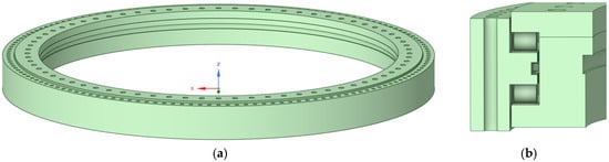
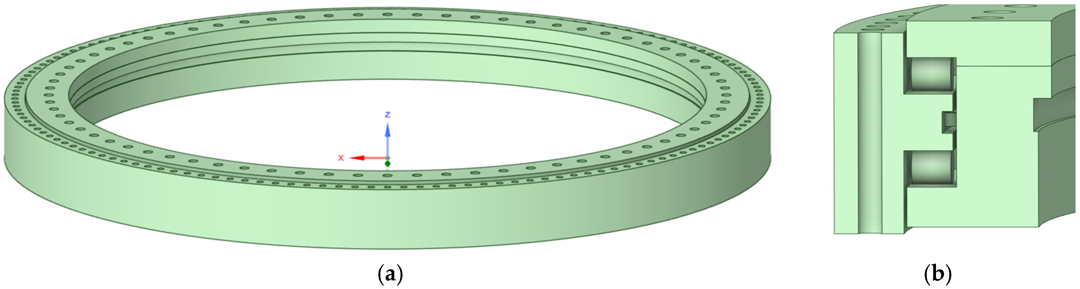
Unlike typical high-speed rotating bearings, slewing bearings for wind turbines are designed to withstand high overturning moments due to the large distance between the support point and the load application point. Due to these structural characteristics, extremely high contact stresses and cyclic loads occur in the contact area, requiring sufficient load-bearing capacity. 42CrMo4 alloy steel is commonly used as the material for slewing bearings in wind turbines. To ensure contact fatigue life, the material must be sufficiently hardened not only on the raceway surface but also in the stress-induced zone beneath the surface. Accordingly, the 4 MW-class pitch bearing under study must meet a minimum surface hardness of 58 HRC and a required hardening depth of at least 6 mm, in accordance with design and quality requirements. Since the raceway has a repetitive pattern in the circumferential direction, a TRB (Triple Roller Bearing)-based analysis model was developed for a representative section to improve computational efficiency. The bearing geometry used in the analysis is shown in Figure 1, and the main dimensions are listed in Table 1. The bearing geometry used in the analysis was modeled using Ansys SpaceClaim 2025 R2 (ANSYS, Inc., Canonsburg, PA, USA), as shown in Figure 1, and the main dimensions are listed in Table 1.
Figure 1.
Pitch bearing geometry in wind turbine generators: (a) overall geometry of wind turbine bearing; (b) cross-sectional geometry.
Table 1.
Main geometric dimensions of the pitch bearing.
2.2. Arrangement of Inductor
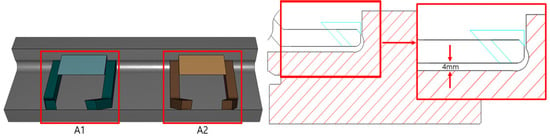
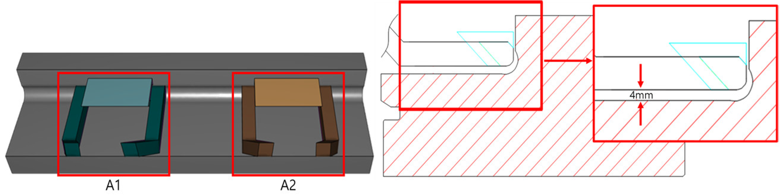
To achieve the target hardening depth, we designed a dual-inductor system incorporating a magnetic flux concentrator made of ferromagnetic metal powder bonded with an organic binder; the inductors were configured to move along the raceway during heating. The air gap between the inductor and the slewing bearing raceway is a key geometric factor that affects the magnetic field distribution and induced current density, and must therefore be taken into account in moving-type induction heating analyses [19,20]. Therefore, taking into account the actual assembly conditions, the potential for interference between the inductor and the workpiece, and local variations in the air gap at the curved ends of the raceway, the average air gap was set to 4 mm. Subsequently, to evaluate changes in temperature distribution and hardening depth resulting from variations in the air gap, air gap conditions ranging from 3 to 5 mm (with 4 mm as the reference) were set as analysis variables. The arrangement and assembly spacing of the dual inductors are shown in Figure 2, and the main dimensions of the dual inductors are listed in Table 2.
Figure 2.
Arrangement of dual inductor position and air gap.
Table 2.
Main dimensions of the dual-inductor configuration.
2.3. Model and Mesh System
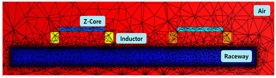
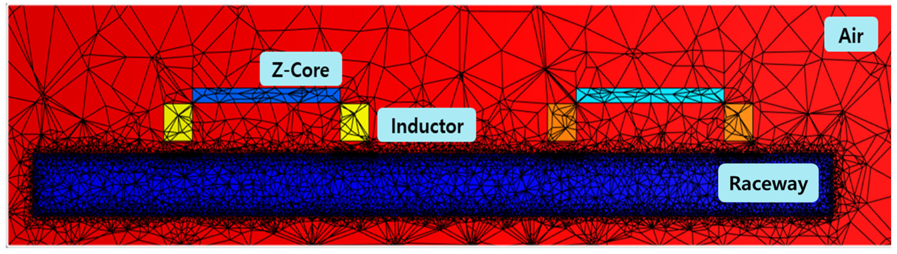
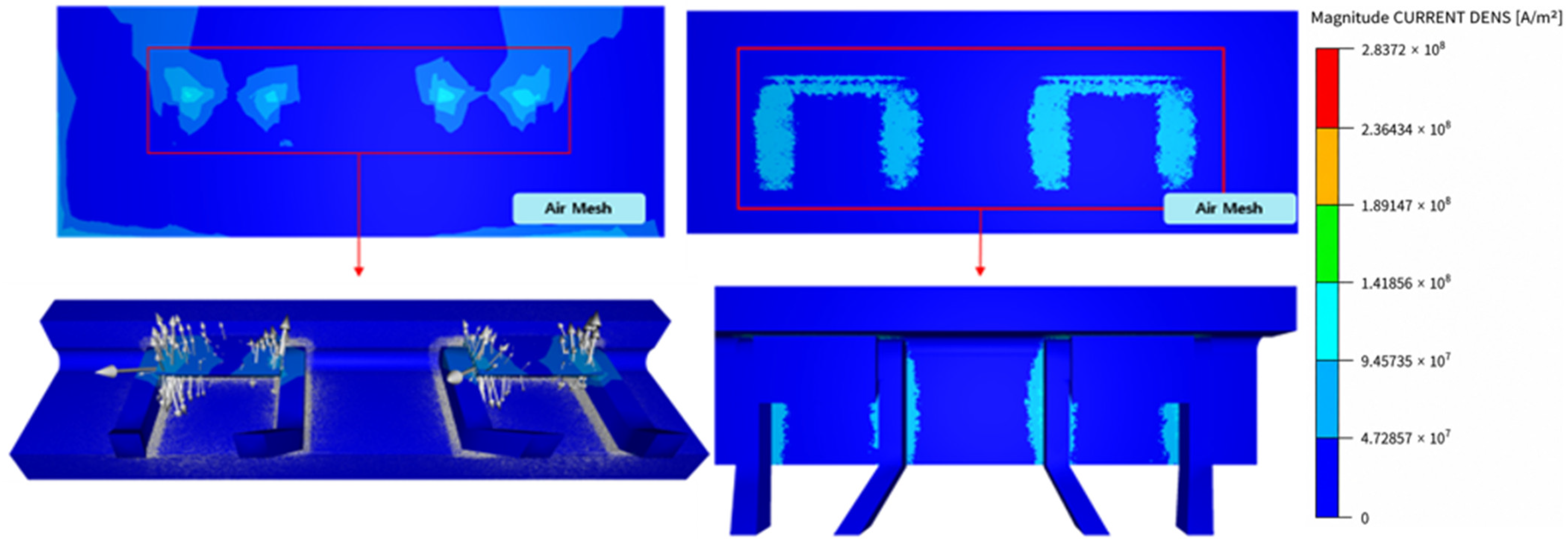
To analyze the electromagnetic field and induction heating behavior of a dual-inductor system incorporating a magnetic flux concentrator, electromagnetic simulation models and induction heating simulation models were developed separately using Forge NxT. The electromagnetic simulation model, based on Maxwell’s equations, was designed to calculate magnetic field distributions and induced current densities, and included the workpiece, inductor, magnetic flux concentrator (Z-Core), and the surrounding air region. The calculated induced current density was then converted into a Joule heating source and applied to the induction heating analysis model, which was used as a thermal analysis model to evaluate the time-dependent temperature distribution and hardening depth of the workpiece.
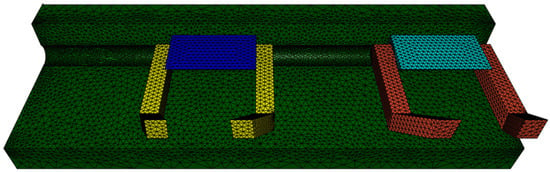
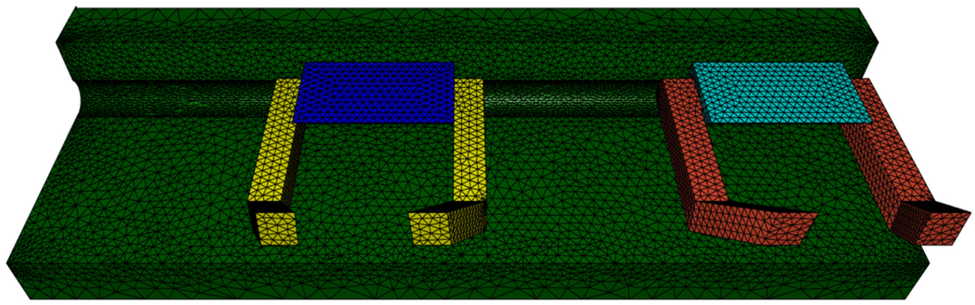
The entire system is surrounded by air. The electromagnetic analysis model consists of a total of 258,835 nodes and 1,662,626 elements; the mesh details are summarized in Table 3, while the mesh configuration is illustrated in Figure 3. The induction heating analysis model consists of a total of 28,872 nodes and 38,256 elements; the mesh information and mesh configuration are presented in Table 4 and Figure 4, respectively. The finite element analysis model was constructed using tetrahedral elements, and adaptive remeshing using Forge NxT was applied to control element distortion. Furthermore, since the time step is automatically adjusted according to the Newton–Raphson convergence criterion, no separate mesh and time step independence analysis was performed.
Table 3.
Mesh configuration of the 3D mobile inductor electromagnetic computation model.
Figure 3.
Cross-sectional mesh configuration of the electromagnetic computation model.
Table 4.
Mesh configuration of the 3D mobile inductor heating computation model.
Figure 4.
Three-dimensional mesh configuration of the dual-inductor heating model.
2.4. Electromagnetic and Thermal Properties
The initial conditions were set such that both the ambient temperature and the initial temperature of the workpiece were 25 °C. The convection boundary is defined as the surface of the workpiece and is expressed in the thermal analysis as shown in Equation (2). The heat transfer coefficient (HTC) at the workpiece surface is 20 W/(m2·K), and the radiative heat loss coefficient is 0.5 W/(m2·K4).
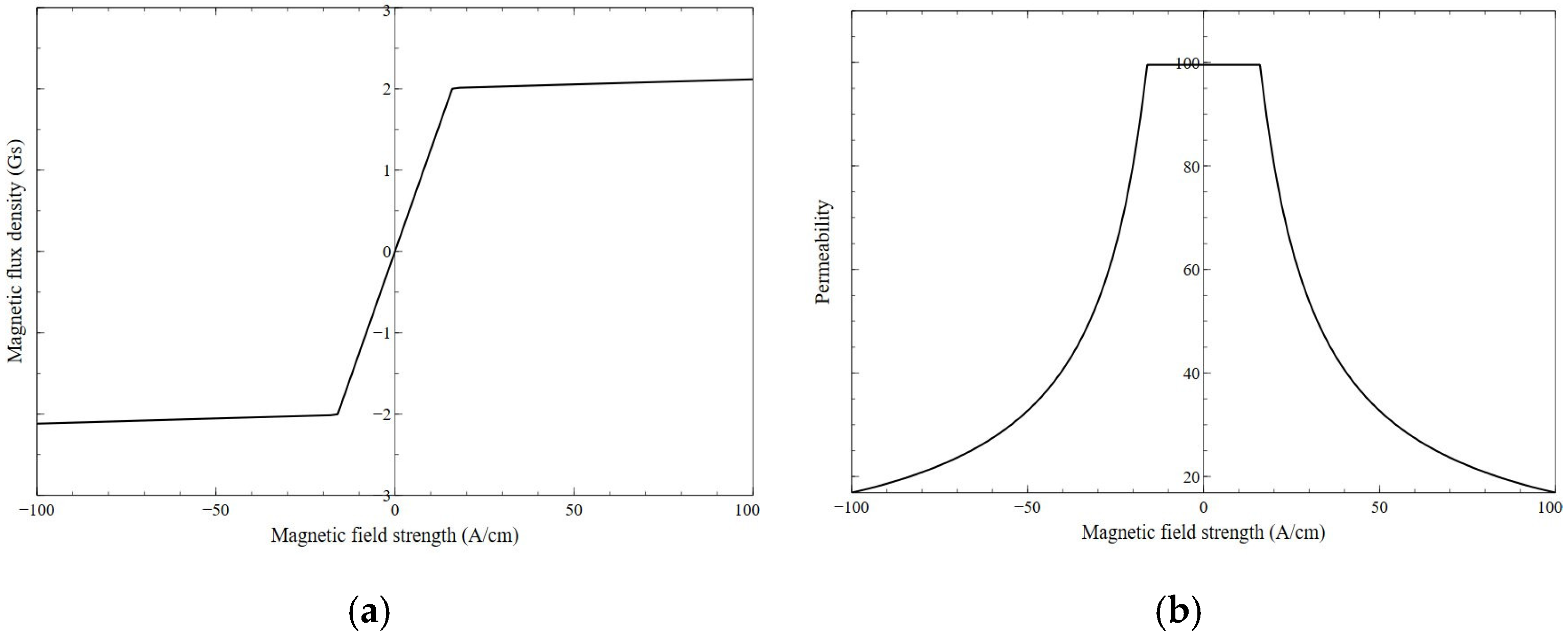
Here, ∂T/∂n is the temperature gradient perpendicular to the surface of the metal workpiece at the point under consideration, Ta is the initial temperature of the surrounding air, λ is the thermal conductivity of the workpiece, α is the convective surface heat transfer coefficient, C is the radiative heat loss coefficient, and n represents the normal to the workpiece boundary surface. The finite element model was configured to perform electromagnetic–thermal coupled analysis. The temperature-dependent thermal, electrical, and magnetic properties of the workpiece and the inductor, including the variations in electrical conductivity and magnetic permeability at elevated temperatures, were incorporated using the material property data implemented in Forge NxT. In this study, we referred to the B-H curves and permeability data presented by Li et al. [12] to account for the nonlinear behavior of the ferromagnetic flux concentrator.
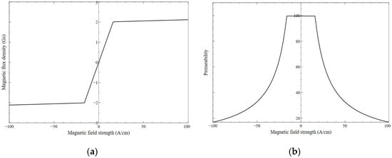
The B-H curve and relative permeability variation in the 42CrMo4 workpiece, which characterize its magnetic properties, were obtained from the Forge NxT material database and are shown in Figure 5.
Figure 5.
Electromagnetic properties of 42CrMo4: (a) B-H curve of 42CrMo4; (b) permeability of 42CrMo4.
The workpiece used in this study is made of 42CrMo4 steel, and its chemical composition is shown in Table 5.
Table 5.
Chemical composition of 42CrMo4 steel (wt.%).
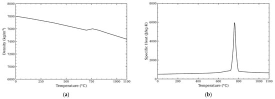
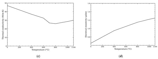
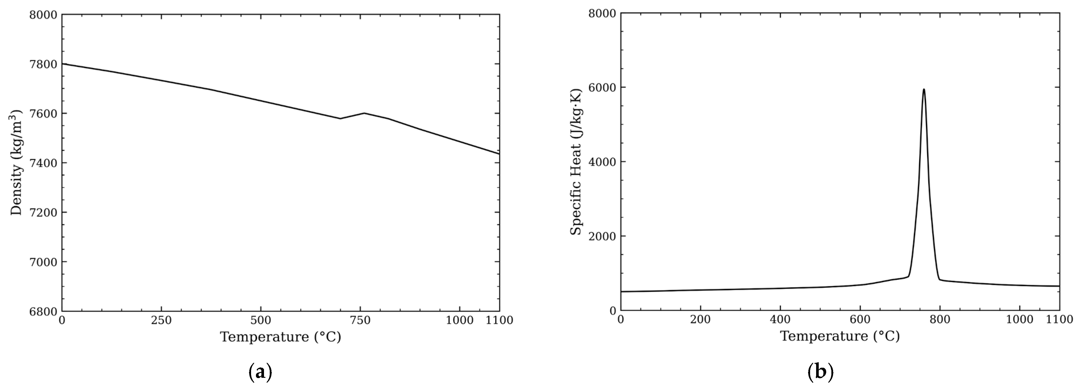
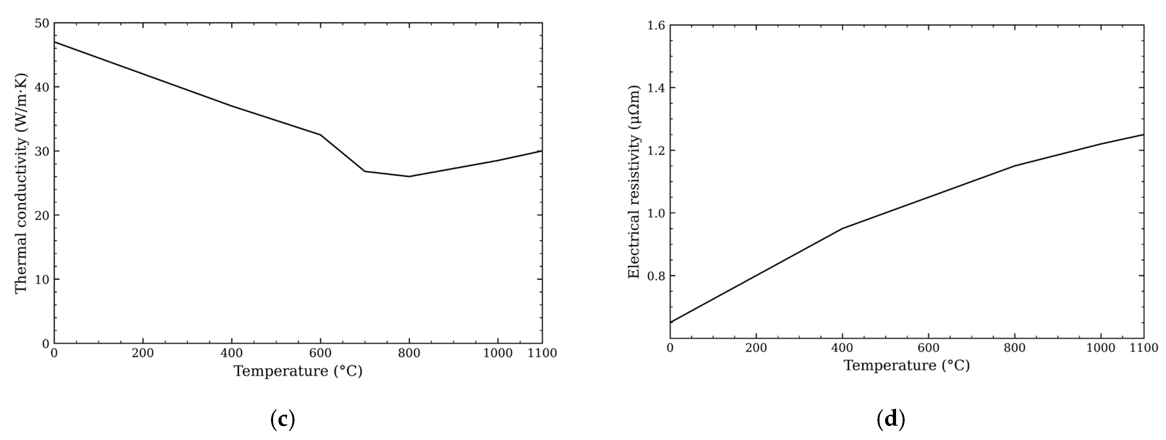
Figure 6 shows the temperature-dependent variations in density, specific heat, thermal conductivity, and electrical resistivity required for heat transfer analysis following induction heating and subsequent cooling. For induction heating heat treatment, the microstructure must be cooled after complete austenitization has occurred. Because the complete austenitization temperature of 42CrMo4 is 770 °C∼820 °C, the target heating temperature was set to be over 820 °C.
Figure 6.
Temperature-dependent thermophysical and electrical properties: (a) density changes with temperature; (b) specific heat changes with temperature; (c) thermal conductivity changes with temperature; and (d) electrical resistivity with temperature.
2.5. Induction Heating Parameters and Input Data for Finite Element Analysis
Using Equation (3), which converts the heat Q applied over a certain time t into power, the required heating power was calculated to be approximately 20,000 W in order to meet the hardness and hardening depth requirements for the heat treatment of the slewing bearing. The frequency can be roughly estimated using the skin effect Equation (1). It can be seen that a frequency of approximately 3080 Hz is required when heating to 820 °C in order to achieve the desired hardening depth. Because the dual inductors are equipped with magnetic flux concentrators, the actual hardening depth may differ from the value estimated only from the penetration depth equation.
Here, m represents mass (kg), represents specific heat , and and represent the uniform temperatures (°C) before and after heating, respectively.
To reduce computational cost, the FEA was performed using a representative 5° sector of the bearing rather than the full bearing geometry. Because the hardening depth of the bearing raceway is strongly affected by the local heating temperature, the temperature difference between the edge and center regions of the heated raceway was considered in the analysis. After setting the heat-treatment conditions so that both areas reached temperatures of 820 °C or higher, the corresponding hardening depths were compared.
The selected process variables were the air gap and the current distribution between the dual inductors. The air gap was set to three values of 3, 4, and 5 mm, and the current applied to each inductor was varied within the range of 7000–9000 A.
Given the high computational cost of analyzing transient induction heating and cooling, representative conditions were selected from the full set of variable combinations to construct the analysis cases; the detailed conditions are summarized in Table 6. Here, A1 and A2 represent the current values applied to the first and second inductors, respectively. Conditions in which a high current was concentrated in a single inductor were not considered because they can increase the risk of localized overheating or surface melting. Using the trained DNN model, the reference air gap of the actual equipment was fixed at 4 mm, and the hardening depth was predicted by varying A1 and A2 at regular intervals within the range of 7000–8800 A. Conditions exceeding 8800 A were excluded due to the risk of overheating and surface melting, and the process conditions that met the minimum required hardening depth of 6.0 mm while coming closest to the target value of 6.20 mm were selected as candidate process conditions.
Table 6.
Induction heating parameter.
To replicate the rapid cooling behavior of the heated billet while maintaining computational efficiency, a heat transfer coefficient of 5000 W/(m2·K) for spray cooling was applied. Although a value of 7100 W/(m2·K) higher than 5000 W/(m2·K) was proposed in previous studies, this value was set considering that the cooling capacity would be somewhat reduced due to the open-air nature of the spray cooling [21,22].
The main input conditions for the finite element analysis are presented in Table 7. Figure 7 shows the magnetic flux distribution calculated from the induction heating analysis, which was used to identify the heating zone and the energy concentration region between the workpiece and the inductors.
Table 7.
Input conditions for finite element analysis.
Figure 7.
Magnetic flux distribution in the induction heating analysis.
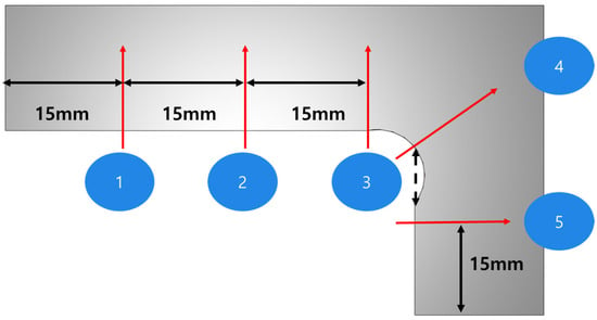
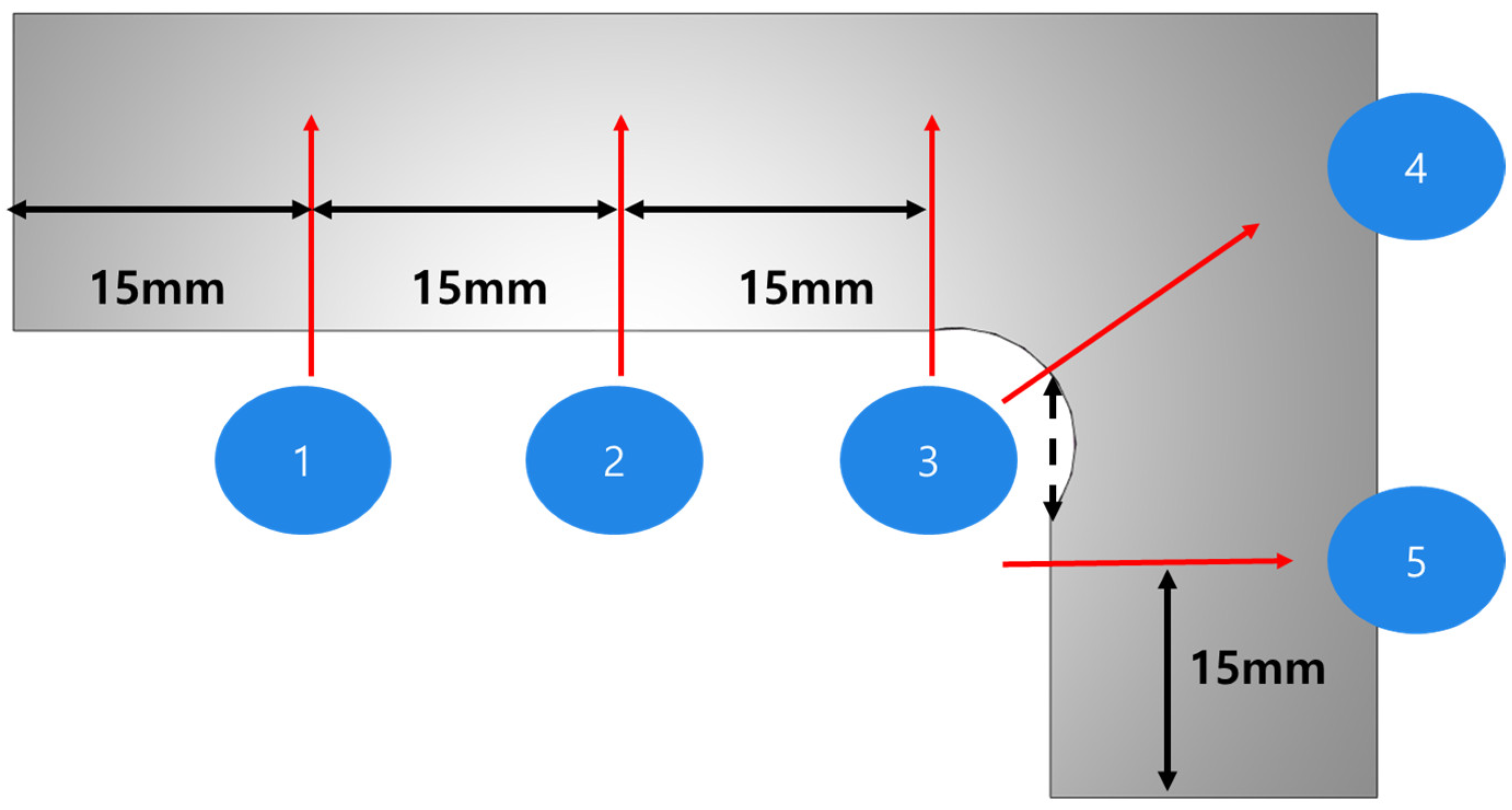
Based on the results of the finite element analysis, five locations were identified to determine the hardening depth, as shown in Figure 8.
Figure 8.
Measurement locations for comparing hardening depth.
2.6. Phase-Transformation Kinetics and Evaluation Criteria
Phase transformation behavior was calculated based on the 42CrMo4 heat-treatment database built into the Forge NxT Heat-Treatment Module. The JMAK model was applied to diffusion-controlled phase transformations such as ferrite, pearlite, and bainite, and the transformation fraction is expressed as follows.
Here, is the phase transformation fraction of phase i, is the maximum phase transformation fraction, and and are temperature-dependent kinetic coefficients. In the non-isothermal induction heating and cooling process, the phase fractions were calculated incrementally based on the time–temperature history at each integration point [1]. A similar Avrami-based phase transformation calculation has also been applied in the analysis of induction hardening of 42CrMo steel.
During cooling, when the temperature drops below the martensite start temperature M_s, the retained austenite transforms into martensite according to the Koistinen–Marburger model.
Here, is the martensite fraction, is the austenite fraction formed prior to cooling, and is the current temperature. Therefore, the final martensite fraction is influenced not only by the cooling rate but also by the austenite fraction formed during heating and the cooling temperature history [8].
In this study, the austenitization evaluation criterion for 42CrMo4 steel was set at 820 °C. However, the presence of complete austenitization was not determined solely by whether the temperature reached 820 °C; instead, it was evaluated based on the austenite volume fraction calculated at each location. The characteristic temperatures for the major phase transformations are summarized in Table 8.
Table 8.
Characteristic phase-transformation temperatures of 42CrMo4 used in the heat-treatment analysis.
2.7. Proxy Model Construction and Small-Sample Validation Strategies
A DNN model was applied to predict the hardening depth in the induction heating process. Considering the selected process variables, the air gap and the currents applied to the two inductors (A1 and A2) were used as input variables, while the hardening depth at each measurement location was used as the output variable. The entire dataset was split into a 70% training set and a 30% test set through random sampling. The parameters for the DNN model are shown in Table 9, and training and prediction performance evaluations were conducted using a total of eight FEA data points. Since only a total of eight FEA cases were available, the DNN comprising three hidden layers with 30 nodes per layer exhibits high model complexity relative to the amount of data. Therefore, the DNN results were not interpreted as evidence of statistically robust generalization performance, but were limited to being interpreted as proxy model results for exploring candidate conditions within the investigated process range.
Table 9.
DNN model architecture.
To examine whether the prediction results of the DNN are overly dependent on a specific model structure under limited sample conditions, RSM, GPR, and SVR were added as comparative surrogate models. All models used the air gap, A1, and A2 currents as input variables, and the hardening depth at position 4 where the minimum hardening depth occurred as the output variable. The RSM was composed of linear terms and two-factor interaction terms. LOOCV using eight FEA cases was applied to the RSM, GPR, and SVR. In each iteration, the model was trained on seven cases and validated on the remaining one, yielding a total of eight out-of-fold predictions, which were used to calculate R2, RMSE, and MAE.
3. Results
3.1. Finite Element Analysis Result
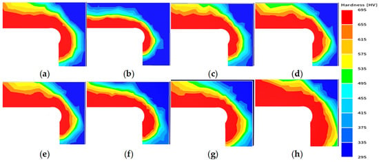
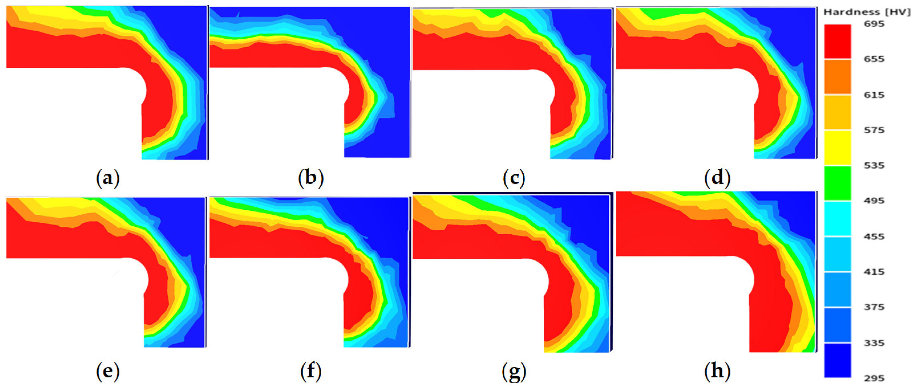
Finite element analysis was performed to examine the temperature distribution and hardening depth during the induction heating process. The analysis was conducted by setting the air gap and current (A1, A2) as process variables, and the results showed that the shape and depth of the hardened zone tended to vary with changes in these variables. Table 10 lists the hardening depths based on the depth at which the hardness remains at or above 550 HV, based on results obtained by considering the air gap and current, while Figure 9 shows the hardness distribution.
Table 10.
FEA result value.
Figure 9.
Hardness distribution after induction hardening calculated by FEA: (a) 3-8000-8000; (b) 4-7000-7000; (c) 4-7000-8000; (d) 4-7000-9000; (e) 4-8000-8000; (f) 5-9000-7000; (g) 5-9000-8000; and (h) 5-9000-9000.
3.2. Comparison of Surrogate Models and Selection of Candidate Process Conditions
According to the FEA results, the lowest hardening depth was observed at position 4 among the five measurement locations, and it was identified as the critical location most likely to fall short of the minimum required hardening depth. Therefore, the hardening depth at position 4 was used as the criterion for comparing the performance of surrogate models and selecting candidate process conditions. The company’s minimum required hardening depth is 6 mm, and the target value was set at approximately 6.2 mm to account for process margins.
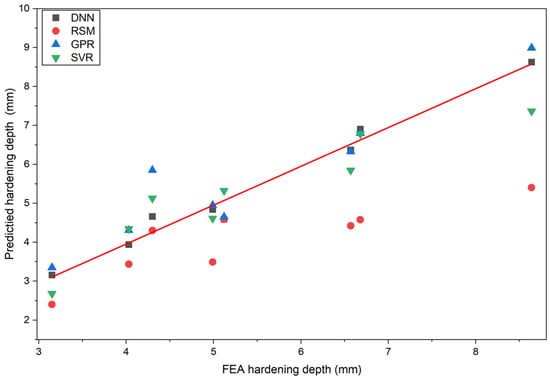
To examine the model dependency of DNN predictions under small-sample conditions, the prediction results of RSM, GPR, and SVR were compared. The four surrogate models generally exhibited similar trends in hardening depth changes; however, differences in over- or under-prediction were observed among the models under certain conditions. The DNN showed relatively good results for some error metrics and in predictions near the target hardening depth. The R2, RMSE, and MAE for each model are summarized in Table 11, and a comparison of the FEA results with the predictions from each model is presented in Figure 10.
Table 11.
Prediction performance of the surrogate models for hardening depth at position 4.
Figure 10.
Parity plot comparing the FEA-calculated and surrogate-model-predicted hardening depths at position 4. The diagonal line represents perfect agreement. .
However, while the DNN’s performance metrics were calculated using a single 70/30 training–test split, the metrics for RSM, GPR, and SVR are based on LOOCV results. Therefore, the values in Table 11 were not interpreted as an absolute model ranking derived from identical validation conditions, and the possibility of DNN overfitting due to the limited sample size was not ruled out. In this study, based on a comprehensive evaluation of the prediction trends, error metrics, and prediction results near the target hardening depth for each model, the DNN was retained as a candidate process condition selection model.
Table 12 presents the predicted hardening depths at position 4 for each candidate process condition evaluated using the DNN. Case 21 exhibited the greatest hardening depth at 7.96 mm; however, under high-current conditions (Gap = 5 mm and A1 = A2 = 8800 A), there is a risk of local overheating, excessive hardening, and increased energy consumption. Therefore, priority was given to conditions that met the minimum requirements at the actual reference air gap of 4 mm rather than the maximum hardening depth—while approaching the target value. Accordingly, Case 15, with A1 = 8200 A and A2 = 8600 A, was selected as the final candidate process condition, and the DNN-predicted hardening depth at position 4 was 6.17 mm.
Table 12.
DNN-predicted hardening depths at position 4 for the evaluated process conditions.
3.3. Finite Element Validation
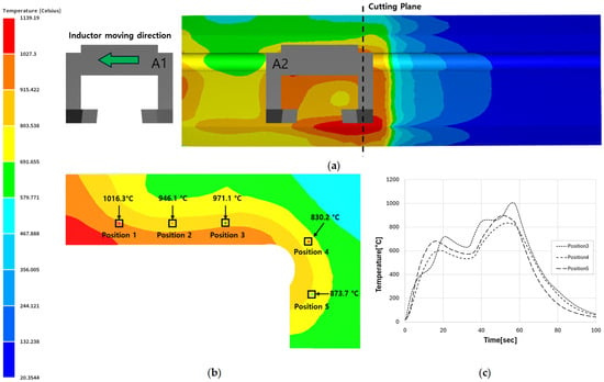
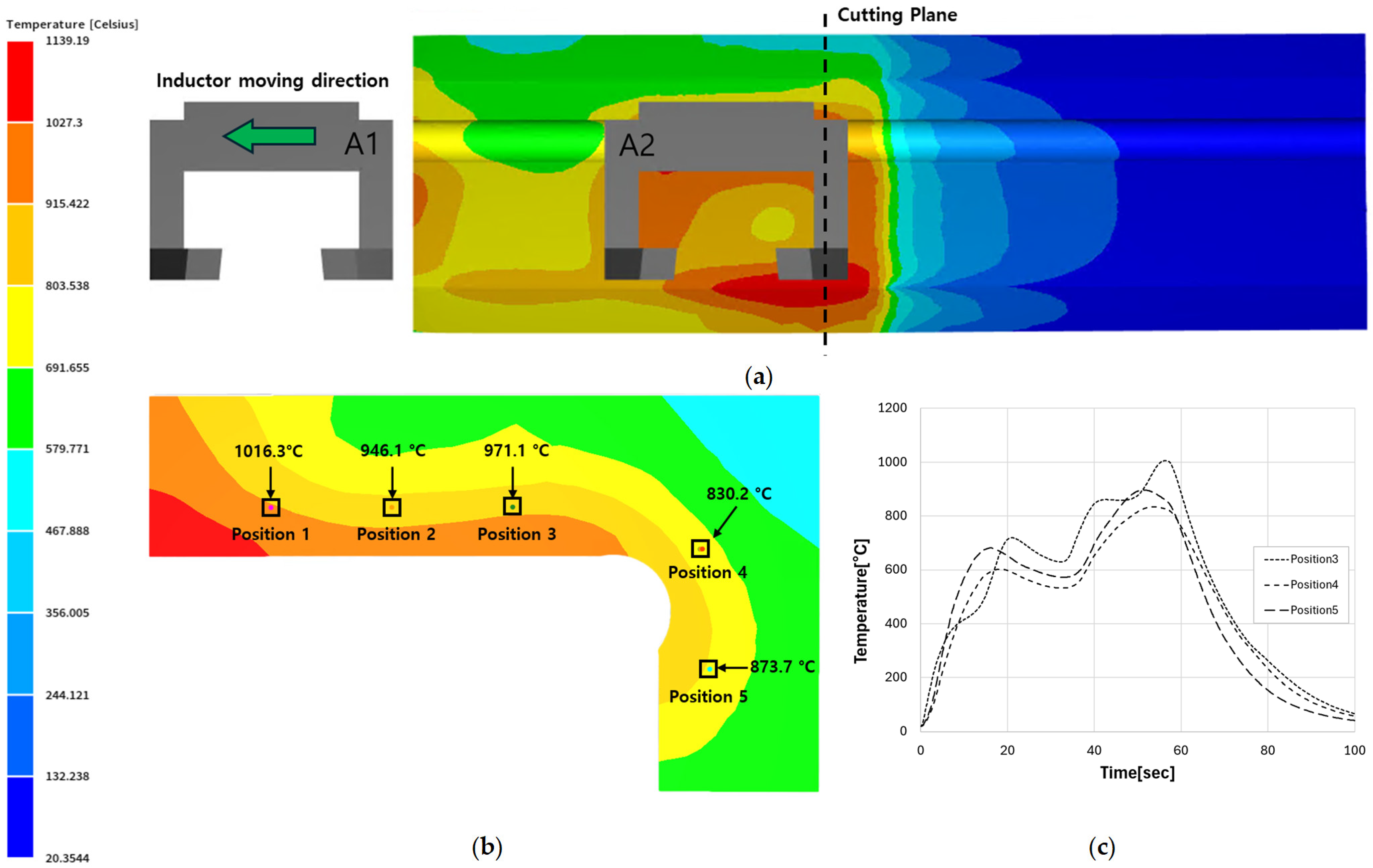
Finite element analysis was performed for the selected induction heating conditions, and the temperature history, phase transformation behavior, and hardening characteristics at positions 1–5 were analyzed. Figure 11a shows the temperature analysis results as the moving inductor progressed, along with the cross-sectional locations used to analyze the temperature, hardness, and phase fraction in the subsurface region. Figure 11b shows the temperature distribution across the cross-section and the temperatures at the evaluation positions. The maximum temperatures at positions 1–5 were calculated to be 1016.3 °C, 946.1 °C, 971.1 °C, 830.2 °C, and 873.7 °C, respectively. The analysis results showed that the lowest temperature was observed at position 4, located in the curved section. Figure 11c shows the temperature changes at each position—positions 3–5—during the process from heating to cooling.
Figure 11.
Finite element analysis results for induction hardening conditions selected using a surrogate model: (a) 3D induction heating analysis results and cutting position; (b) temperature distribution of section plane; and (c) time-dependent temperature variations at different locations during heating and cooling.
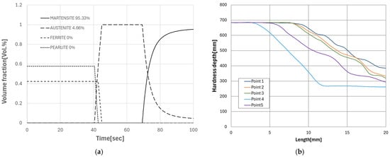
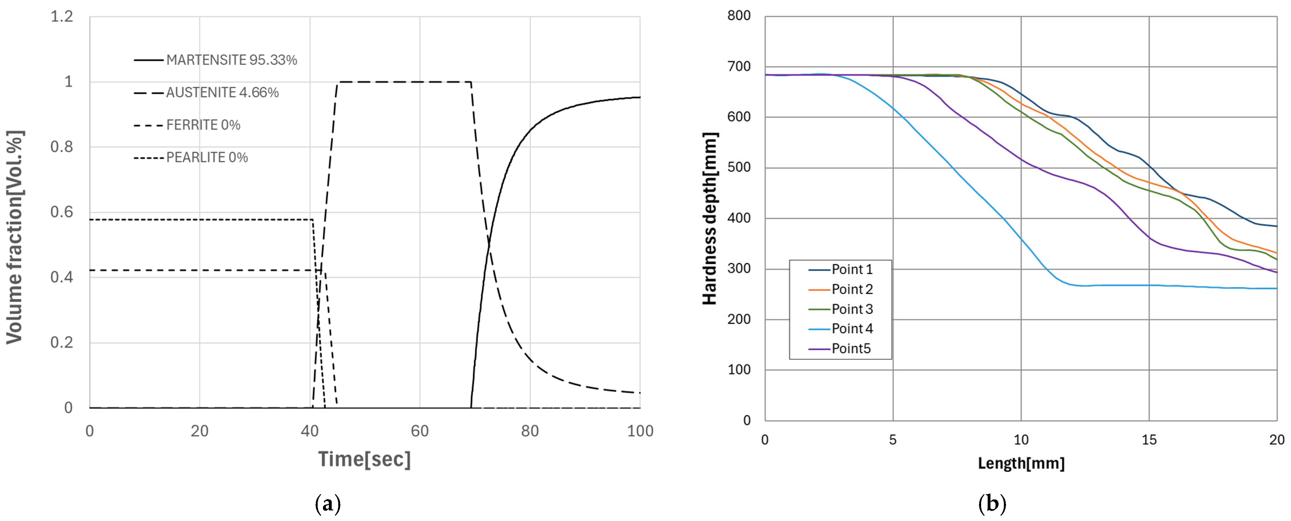
Figure 12a shows the evolution of phase fractions over time at position 4. During heating, austenite was formed as the initial ferrite and pearlite depleted, and during cooling, the austenite transformed into martensite. Upon completion of cooling, the final microstructure at position 4 comprised 95.33% martensite and 4.67% retained austenite. This confirms that austenitization and martensitic transformation occurred sufficiently in the surface region at position 4.
Figure 12.
Finite element analysis results for microstructure fraction and hardness: (a) microstructure fraction of position 4; (b) hardness distribution with depth at each position.
Figure 12b shows the final hardness distribution as a function of depth from the surface at positions 1–5. While the surface hardness across all positions was consistently around 680 HV, a distinct difference was observed in the hardness reduction profiles with increasing depth. The effective hardening depth, defined at a threshold of 550 HV, was 13.63 mm, 13.41 mm, 9.47 mm, 6.38 mm, and 9.49 mm at positions 1–5, respectively, with position 4 exhibiting the minimum hardening depth.
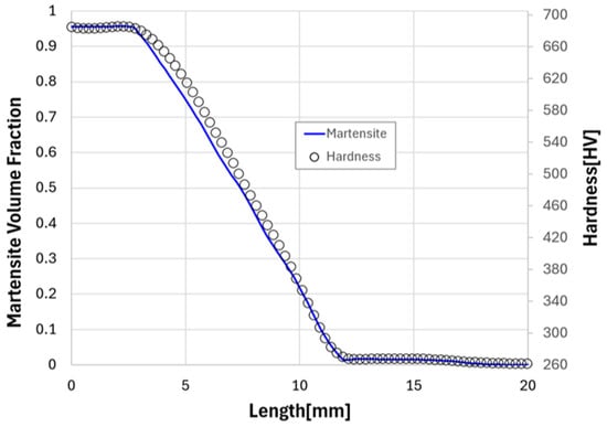
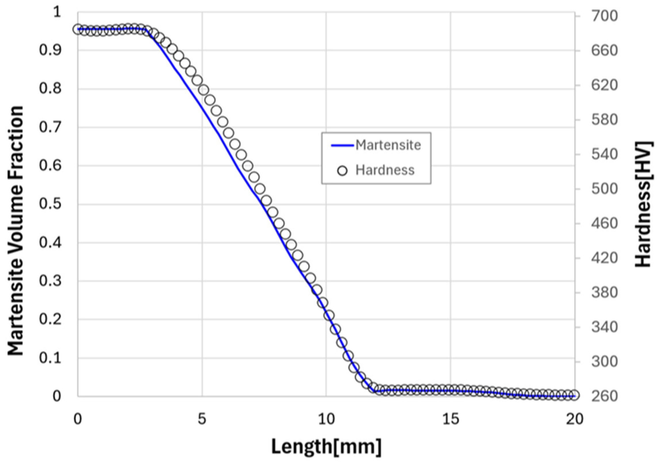
Figure 13 shows the relationship between the final martensite volume fraction and the hardness distribution as a function of depth from the surface at position 4. It can be observed that while a high martensite fraction and hardness were maintained near the surface, the martensite fraction decreased toward the interior, and hardness also decreased accordingly.
Figure 13.
Hardness and martensite fraction profiles as a function of depth from the surface calculated by finite element analysis.
4. Discussion
In the FEA results, position 4 exhibited a relatively shallow hardening depth in all analysis cases and was identified as the critical location most likely to fall short of the minimum required hardening depth. These results can be explained by changes in the effective air gap due to the local curvature of the raceway and the relative positioning between the inductor and the workpiece. In curved sections, the distribution of the magnetic field and induced current density becomes more uneven compared to straight sections; consequently, localized temperature rises may occur, and the austenitization zone may be restricted. Since the martensite zone formed during the subsequent cooling process is also reduced, it is concluded that a relatively shallow hardened layer formed at position 4. In an additional finite element analysis of the selected induction heating conditions, the maximum temperature at position 4 was calculated to be 830.2 °C, the lowest among the five positions. After cooling, 95.33% martensite was formed at the evaluation point in that location, and the surface hardness reached approximately 680 HV; however, both the martensite fraction and hardness decreased as one moved from the surface toward the interior, limiting the effective hardening depth to 6.38 mm. Although the hardening characteristics of the surface layer were secured at position 4, the formation of the hardened layer in the depth direction was constrained due to the relatively low local heating temperature. This demonstrates that when evaluating induction hardening process conditions for large slewing bearings, priority should be given to the minimum hardening depth at geometrically vulnerable locations rather than the average or maximum hardening depth.
A comparison of the prediction results from RSM, GPR, SVR, and DNN using the same FEA process conditions showed that each model generally exhibited similar overall trends in the increase or decrease in hardening depth in response to changes in process variable combinations. However, there were differences in the quantitative prediction values and error metrics; in particular, the RSM tended to underestimate the hardening depth in the high-depth range. The GPR and SVR exhibited relatively similar predictive performance, while the DNN showed numerically low RMSE and MAE in a single 70/30 split and produced relatively good predictions even near the target hardening depth of 6.20 mm. However, since the DNN metrics were calculated from a single training–test split, while the RSM, GPR, and SVR metrics were derived from out-of-fold predictions in LOOCV, these results cannot be interpreted as an absolute model ranking obtained under identical validation conditions.
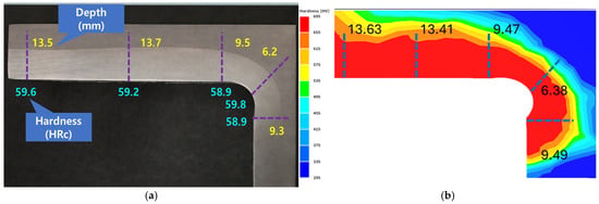
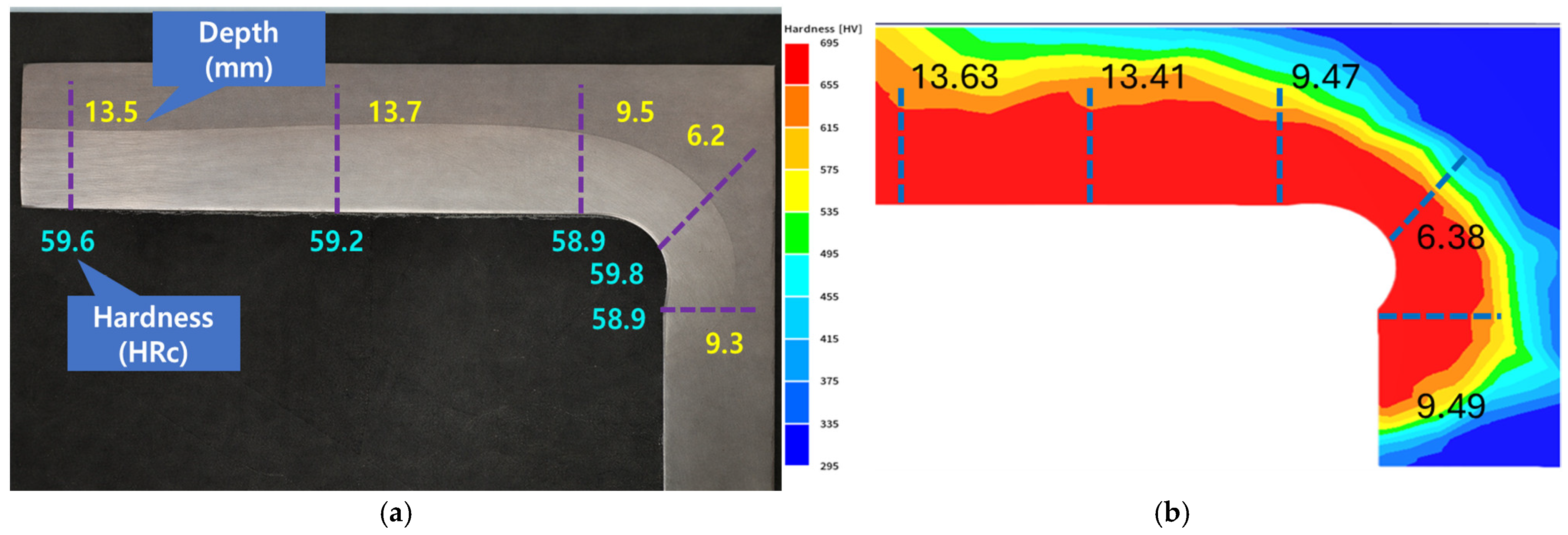
Accordingly, the DNN was not selected as a model that is generally superior to other surrogate models, but was retained as a surrogate model to identify candidate conditions close to the target hardening depth within the investigated process range. At the standard air gap of 4 mm for the actual equipment, the hardening depth at position 4 under the conditions A1 = 8200 A and A2 = 8600 A was predicted by the DNN to be 6.17 mm. To evaluate the feasibility of the selected candidate conditions, additional FEA results were compared with the measured hardening depth, as shown in Figure 14 and Table 13. The additional FEA results and measured values at position 4 were 6.38 mm and 6.20 mm, respectively, and a generally similar hardening depth distribution was observed across all five measurement positions. Both sets of results satisfied the minimum required hardening depth of 6.0 mm. However, this comparison was interpreted not as a validation to demonstrate the DNN’s statistical generalization performance, but rather as a result confirming the applicability of the candidate conditions selected through the surrogate model.
Figure 14.
Comparison of measured data and finite element analysis: (a) induction heating image provided by the bearing manufacturer; (b) results of finite element analysis based on DNN training.
Table 13.
Measured values and FEA error values.
Previous studies have reported that current, frequency, air gap, coil geometry, and heating and cooling conditions influence the temperature distribution and hardening zone geometry in the induction hardening process, and that linking FEA with data-driven surrogate models can reduce the number of iterative analyses. This study does not propose any new FEA techniques or DNN algorithms either, and in this respect, it is methodologically similar to previous studies. However, this study differs in that it focused on a transient induction hardening process in which an independently controlled dual inductor equipped with a magnetic flux concentrator moves along the raceway of a large-scale slewing bearing. In particular, we evaluated the spatial non-uniformity of hardening depth based on local geometry to identify the critical location where the minimum hardening depth occurs; we then selected candidate process conditions based on this location and compared them with results from additional FEA analyses and experimentally measured hardening depths. Therefore, the main contribution of this study lies not in proposing a new surrogate model or demonstrating the superiority of one model over another, but in the integrated application of transient multiphysics FEA, comparison of multiple surrogate models, condition selection based on critical locations, and subsequent validation to the mobile dual-inductor induction hardening process. However, the FEA data used in this study is limited to a total of eight cases, and the DNN has a relatively complex structure compared to the amount of data. Furthermore, since different validation methods were applied to the DNN and the other surrogate models, it is difficult to claim the general superiority or robust generalization performance of the DNN based solely on the current results. The input variables were also limited to the air gap and the currents in the two inductors, so the effects of frequency, inductor travel speed, heating time, and cooling conditions were not included. Furthermore, the quantitative experimental validation in this study was limited to effective hardening depth, a key quality criterion in industrial settings, and did not verify temperature history during the process, depth-direction hardness profiles, microstructure, or residual stresses. In the future, it will be necessary to expand the number of FEA and experimental data sets and compare models under the same cross-validation conditions, while also evaluating the predictive reliability and scope of application of the models by including additional process variables and measurements of temperature, hardness, microstructure, and residual stress.
5. Conclusions
In this study, we used electromagnetic–thermal–phase-transition coupled transient FEA and surrogate models to identify candidate process conditions that satisfy the target hardening depth for large-scale rotating bearing raceways in wind turbines, which are heated by a moving, independently controlled dual-inductor system equipped with a magnetic flux concentrator. The main conclusions are as follows:
- FEA results confirmed that the air gap and the currents in the two inductors are the primary process variables affecting the temperature distribution and hardening depth of the raceway. Among the five measurement positions, position 4 exhibited the lowest hardening depth and was designated as the critical location most likely to fall short of the minimum requirement.
- RSM, GPR, SVR, and DNN generally showed similar trends in the overall increase or decrease in hardening depth as process variables changed. Although DNN showed relatively good results for some error metrics and near the target hardening depth, it was not interpreted as generally superior to other models, given the small sample size and differences in validation methods.
- At the actual reference air gap of 4 mm, the conditions A1 = 8200 A and A2 = 8600 A were selected as the final candidate process conditions. The hardening depth at position 4 was 6.17 mm according to the DNN, 6.38 mm according to the supplementary FEA, and 6.20 mm according to actual measurements, thereby satisfying the minimum required hardening depth of 6.0 mm. In the additional FEA analysis, the maximum temperature at position 4 was 830.2 °C, the lowest among the five positions, and a martensite fraction of approximately 95.33% and a hardness of approximately 680 HV were formed in the surface region. However, as the depth from the surface increased, both the martensite fraction and hardness decreased, confirming numerically the thermal and metallurgical behavior that results in the shallowest hardened layer forming at Position 4.
- The main contribution of this study lies not in proposing a new learning algorithm, but in the integrated application of transient multiphysics FEA, comparison of multiple surrogate models, selection of candidate conditions based on critical locations, and subsequent verification to the mobile dual-inductor induction hardening process for large slewing bearings. This procedure can be used to select candidate conditions requiring follow-up analysis and experimentation before performing iterative FEA for all variable combinations.
- This study utilized a total of eight FEA cases; however, the verification methods varied by model, and experimental verification was limited to hardening depth. In the future, it will be necessary to expand the FEA and experimental data, incorporate additional parameters such as frequency, travel speed, heating time, and cooling conditions, and conduct comprehensive verification of temperature history, hardness profiles, microstructure, and residual stresses.
Consequently, this FEA-based surrogate modeling procedure can be utilized as a process design support method to efficiently screen candidate process conditions based on the minimum hardening depth in large-scale mobile induction hardening processes.
Author Contributions
Research Concept: Y.-J.A. and J.-H.K.; Research Methodology: Y.-J.A. and J.-H.K.; Software: Y.-J.A.; Validation: Y.-J.A., J.-P.H., and J.-H.K.; Quantitative Analysis: Y.-J.A.; Investigation: Y.-J.A., J.-P.H., H.-S.J., M.-G.K., and S.-H.S.; Resources: J.-H.K.; Data management: Y.-J.A.; Manuscript preparation—drafting: Y.-J.A.; Writing—review and editing: Y.-J.A. and J.-H.K.; Visualization, M.-G.K.; Maps, J.-H.K.; Project management, J.-H.K.; Funding, J.-H.K. All authors have read and agreed to the published version of the manuscript.
Funding
This study was supported by the Korea Institute of Energy Technology Evaluation and Planning (KETEP) grant funded by the Ministry of Trade, Industry and Energy of the Republic of Korea (Project No. RS-2023-00302111).
Data Availability Statement
The original contributions presented in this study are included in the article. Further inquiries can be directed to the corresponding author.
Acknowledgments
This research was conducted with funding from the Korea Energy Technology Evaluation and Planning (KETEP), supported by the Ministry of Trade, Industry and Energy of the Republic of Korea (Grant No. RS**2023-00302111). While writing this paper, the authors used ChatGPT (GPT-5.6 Sol, OpenAI) for grammar checking. After using this tool, the authors reviewed and revised the content as necessary.
Conflicts of Interest
The authors declare no conflict of interest.
Abbreviations
The following abbreviations are used in this manuscript:
| FEA | Finite element analysis |
| DNN | Deep neural network |
| RSM | Response Surface Methodology |
| GPR | Gaussian Process Regression |
| SVR | Support Vector Regression |
| TRB | Triple roller bearing |
| HRC | Rockwell hardness C scale |
| HV | Vickers hardness |
| RMSE | Root mean square error |
References
- Zhong, H.; Wang, Z.; Gan, J.; Wang, X.; Yang, Y.; He, J.; Wei, T.; Qin, X. Numerical simulation of martensitic transformation plasticity of 42CrMo steel based on spot continual induction hardening model. Surf. Coat. Technol. 2020, 385, 125428. [Google Scholar] [CrossRef] [Scilit]
- Maresca, F.; Kouznetsova, V.; Geers, M.; Curtin, W. Contribution of austenite-martensite transformation to deformability of advanced high strength steels: From atomistic mechanisms to microstructural response. Acta Mater. 2018, 156, 463–478. [Google Scholar] [CrossRef] [Scilit]
- Yoshida, W. Residual stress control on bearing steel by surface cooled induction heating fast tempering. J. Mater. Eng. Perform. 2020, 29, 3585–3592. [Google Scholar] [CrossRef] [Scilit]
- Takesue, S.; Ono, K.; Nambu, K.; Kikuchi, S. Fatigue Limit Estimation for Post-Peened Induction-Hardened and Tempered Steel Considering Changes in Surface Properties. Fatigue Fract. Eng. Mater. Struct. 2024, 47, 4607–4617. [Google Scholar] [CrossRef] [Scilit]
- Göncz, P.; Glodež, S. Rolling Contact Fatigue Life Assessment of Induction Hardened Raceway. Procedia Eng. 2014, 74, 392–396. [Google Scholar] [CrossRef] [Scilit]
- Li, H.; He, L.; Gai, K.; Jiang, R.; Zhang, C.; Li, M. Numerical simulation and experimental investigation on the induction hardening of a ball screw. Mater. Des. 2015, 87, 863–876. [Google Scholar] [CrossRef] [Scilit]
- Hömberg, D.; Liu, Q.; Montalvo-Urquizo, J.; Nadolski, D.; Petzold, T.; Schmidt, A.; Schulz, A. Simulation of multi-frequency induction-hardening including phase transitions and mechanical effects. Finite Elem. Anal. Des. 2016, 121, 86–100. [Google Scholar] [CrossRef] [Scilit]
- Tong, D.M.; Gu, J.F.; Yang, F. Numerical simulation on induction heat treatment process of a shaft part: Involving induction hardening and tempering. J. Mater. Process. Technol. 2018, 262, 277–289. [Google Scholar] [CrossRef] [Scilit]
- Fisk, M.; Lindgren, L.E.; Datchary, W.; Deshmukh, V. Modelling of induction hardening in low alloy steels. Finite Elem. Anal. Des. 2018, 144, 61–75. [Google Scholar] [CrossRef] [Scilit]
- Javaheri, V.; Pohjonen, A.; Asperheim, J.I.; Ivanov, D.; Porter, D. Physically based modeling, characterization and design of an induction hardening process for a new slurry pipeline steel. Mater. Des. 2019, 182, 108047. [Google Scholar] [CrossRef] [Scilit]
- Li, F.; Ning, J.; Liang, S.Y. Analytical Modeling of the Temperature Using Uniform Moving Heat Source in Planar Induction Heating Process. Appl. Sci. 2019, 9, 1445. [Google Scholar] [CrossRef] [Scilit]
- Li, F.; Li, X.; Zhu, T.; Rong, Y. Numerical Simulation of the Moving Induction Heating Process with Magnetic Flux Concentrator. Adv. Mech. Eng. 2013, 2013, 907295. [Google Scholar] [CrossRef] [Scilit]
- Mühl, F.; Damon, J.; Dietrich, S.; Schulze, V. Simulation of induction hardening: Simulative sensitivity analysis with respect to material parameters and the surface layer state. Comp. Mater. Sci. 2020, 184, 109916. [Google Scholar] [CrossRef] [Scilit]
- Yamaç, Y.; Özçelik, B. Optimization of Induction Heating Coil in the Surface Hardening Process. J. Aeronaut. Space Technol. 2023, 16, 1–14. [Google Scholar] [CrossRef] [Scilit] [PubMed]
- Derouiche, K.; Garois, S.; Champaney, V.; Daoud, M.; Traidi, K.; Chinesta, F. Data-Driven Modeling for Multiphysics Parametrized Problems-Application to Induction Hardening Process. Metals 2021, 11, 738. [Google Scholar] [CrossRef] [Scilit]
- Garois, S.; Daoud, M.; Chinesta, F. Data-Driven Inverse Problem for Optimizing the Induction Hardening Process of C45 Spur-Gear. Metals 2023, 13, 997. [Google Scholar] [CrossRef] [Scilit]
- Garois, S.; Daoud, M.; Traidi, K.; Chinesta, F. Artificial Intelligence Modeling of Induction Contour Hardening of 300M Steel Bar and C45 Steel Spur-Gear. Int. J. Mater. Form. 2023, 16, 26. [Google Scholar] [CrossRef] [Scilit]
- Cong, H.; Wang, B.; Wang, Z. A Novel Gaussian Process Surrogate Model with Expected Prediction Error for Optimization under Constraints. Mathematics 2024, 12, 1115. [Google Scholar] [CrossRef] [Scilit]
- Meunier, G. The Finite Element Method for Electromagnetic Modeling; ISTE Ltd.: London, UK, 2008; 832p, Available online: https://www.wiley.com/en-us/The+Finite+Element+Method+for+Electromagnetic+Modeling-p-9781848210301 (accessed on 13 May 2020).
- Edali, M.; Yücel, G. Automated Analysis of Regularities Between Model Parameters and Output Using Support Vector Regression in Conjunction with Decision Trees. J. Artif. Soc. Soc. Simul. 2018, 21, 1. [Google Scholar] [CrossRef] [Scilit]
- Zhou, X.; Thomas, B.G.; Hernández, C.A.; Castillejos, A.H.; Acosta, F.A. Measuring heat transfer during spray cooling using controlled induction-heating experiments and computational models. Appl. Math. Model. 2013, 37, 3181–3192. [Google Scholar] [CrossRef] [Scilit]
- Chabičovský, M.; Raudenský, M. Experimental investigation of spray cooling of horizontally and vertically oriented surfaces. In Proceedings of the 22nd International Conference on Metallurgy and Materials—METAL 2013, Brno, Czech Republic, 15–17 May 2013; Tanger Ltd.: Ostrava, Czech Republic, 2013; pp. 102–107. [Google Scholar]

Disclaimer/Publisher’s Note: The statements, opinions and data contained in all publications are solely those of the individual author(s) and contributor(s) and not of MDPI and/or the editor(s). MDPI and/or the editor(s) disclaim responsibility for any injury to people or property resulting from any ideas, methods, instructions or products referred to in the content. |
© 2026 by the authors. Licensee MDPI, Basel, Switzerland. This article is an open access article distributed under the terms and conditions of the Creative Commons Attribution (CC BY) license.