Unloading Acceleration Driven by Shock Pressure: A Theoretical Model for Jet Formation of High Entropy Alloys

Abstract

Accurately predicting the terminal state of shaped charge jets (SCJs) is crucial for optimizing their penetration performance. The core challenge lies in a deep understanding of the complete physical chain from shock compression to unloading expansion. This paper presents a hybrid analytical–numerical model for SCJ formation that incorporates a shock-pressure-driven unloading term. Unlike classical PER theory, the proposed model explicitly introduces an unloading term and derives a quantitative expression for the momentum conversion factor $\left({\Pi }_{DMCF}\right)$ to quantitatively characterize the momentum redistribution during collapse. Our analysis finds that ${\Pi }_{DMCF}$ exhibits a typical S-shaped evolution law as the dimensionless Mach number $\left(Ma\right)$ varies. This study uses a logistic function with two characteristic parameters, $M{a}_0$ and $k$, to accurately fit the data. The research results indicate that the model parameters have clear physical connotations: $M{a}_0$ characterizes the critical condition for the material to transition from “strength-dominated” to “kinetic-energy-dominated” behavior, while k reflects the degree of abrupt transition. After calibrating the model parameters using high-fidelity numerical simulations, the jet morphology and velocity data obtained from X-ray flash photography experiments are compared and verified, confirming that the model can significantly improve the prediction accuracy. Especially for Ti₅₅Al₂₀V₅Zr₅Nb₁₅ HEA, the prediction error in the jet velocity is less than 4%, and the theoretically predicted shock pressure is highly correlated with the numerical results $\left({\mathrm{R}}^2=0.943\right)$. A further mechanistic analysis indicates that the proposed model successfully decodes the unique response of the HEA: its high dynamic strength results in a larger value, causing its momentum conversion efficiency to fall within a lower range under typical impact conditions. The theoretical framework constructed in this study provides a hybrid analytical–numerical and highly reliable theoretical tool for the accurate prediction of SCJs, as well as for the material selection and design of high-performance liners.

1. Introduction

Shaped charge technology is widely used in military and civilian engineering fields due to its ability to generate highly penetrative metal jets [1,2,3,4,5,6]. The terminal penetration performance of a jet largely depends on its initial mass and velocity distribution [7,8,9,10,11]. This is essentially the result of the efficient conversion of normal momentum into axial jet momentum during axisymmetric collapse, driven by the explosive detonation of the shaped charge (SC). Therefore, a deep understanding and precise quantification of this momentum-conversion mechanism are key scientific prerequisites for optimizing SC design and improving penetration efficiency.

The theoretical study of jet formation has always been a popular research topic [12]. The ideal fluid PER theory established by Birkhoff et al. [13] serves as a milestone. The model treats the liner material as an inviscid, incompressible fluid and successfully predicts the velocity and mass distributions of the jet and slug, laying the theoretical foundation for the field. However, treating the material as an ideal fluid without strength neglects the unloading and pressure-release processes after shock compression. In fact, during the collapse of the liner to form a jet, the material first undergoes shock compression and stores enormous energy; subsequently, under the action of sparse waves, the stored energy is released and converted into kinetic energy, resulting in a significant additional acceleration of the jet. Therefore, the final velocity of the jet is determined not only by the collision geometry but also by the complete process of “shock-unloading”.

To more accurately predict jet velocity, the subsequent research has primarily focused in two directions. On the one hand, by integrating complex material equation of state (EOS) and constitutive models with high-fidelity numerical values, it is possible to finely characterize the shock and unloading processes [14,15,16,17]. Despite their strong predictive ability, numerical methods have inherent limitations, including high computational costs, heavy dependence on model parameters and algorithms, and difficulty in providing clear physical mechanisms and universal design criteria. On the other hand, a series of improved analytical or semi-analytical models have been proposed to balance physical transparency and computational efficiency [18,19,20]. These models rely on improved collapse-velocity models and effective charge structures to predict jet velocity from charge-structure parameters [21,22,23].

However, most of the existing analytical or semi-analytical models simplify the handling of the unloading acceleration steps [24,25,26]. This leads to two core issues: first, it is not clear how shock pressure specifically drives unloading acceleration, and second, the quantitative relationship between them is physically opaque. The contribution of the unloading acceleration is difficult to separate from the overall velocity for independent analysis and optimization, hindering the model from clearly revealing the differential mechanism underlying the jet performance of high-strength and high-impedance materials. Therefore, establishing a quantitative model with “shock pressure-unloading acceleration” as the core driving mechanism, clear physical images, and no dependence on specific constitutive models is an urgent need to deepen the understanding of the jet formation mechanism and achieve accurate prediction.

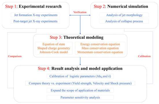
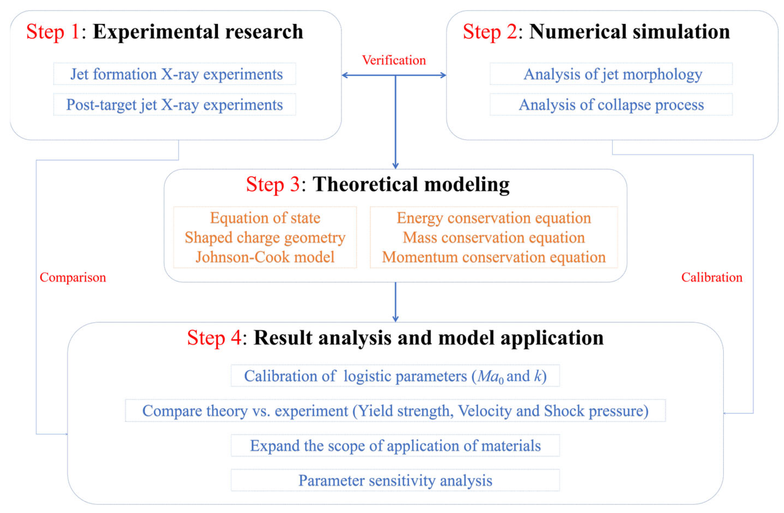
This article proposes a new theoretical model focusing on the physical mechanism of “shock-pressure-driven unloading acceleration”. Figure 1 presents the four main steps of this study in a flowchart format. In Step 1, this article obtains the characteristic parameters of the jet through jet formation and post-target jet X-ray experiments. In Step 2, this article obtains the shape and key parameters of the jet (such as velocity, temperature, yield strength, and pressure) through high-fidelity numerical simulation. In Step 3, this article establishes a theoretical model based on the equation of state, the structure of the shaped charge, and the Johnson–Cook model, combined with the conservation equations of energy, mass, and momentum. In Step 4, this article calibrates the logistic parameters based on high-fidelity numerical simulation results, compares and analyzes the differences between the theoretical and the experimental results, and expands the material applicability of the model and conduct parameter sensitivity analysis to ensure the reliability of the model.

Figure 1. Method framework.

This work presents two distinct advances over the existing SCJ models: first, a shock-pressure-driven unloading term is introduced into the momentum conservation framework with a quantitatively calibrated momentum conversion factor, capturing the energy transfer from the shock state to final jet velocity—a mechanism absent in classical PER theory and its strength-corrected variants; second, instead of adjusting the coefficients within the PER framework, we introduce a new physical term directly into the momentum equation, enabling the prediction of phenomena, such as pressure and temperature distribution and velocity up-estimation, that strength corrections alone cannot explain. These contributions provide new ideas and perspectives for the study of jet formation mechanisms.

2. X-Ray Experiments Method and Results

Ti₅₅Al₂₀V₅Zr₅Nb₁₅ HEA have high strength and good ductility [8]. Therefore, this section obtained the jet morphology of Ti₅₅Al₂₀V₅Zr₅Nb₁₅ HEA and the jet morphology characteristics after penetrating the C45 steel target through X-ray experiments. The destructive and secondary destructive capabilities of the jet are verified by the damage observed on C45 steel targets and combustibles. The structure of the energy gathering charge used in the two experiments is the same as that in references [8,27], in order to facilitate better comparison and analysis of jet morphology.

2.1. Preparation for Jet Formation X-Ray Experiments

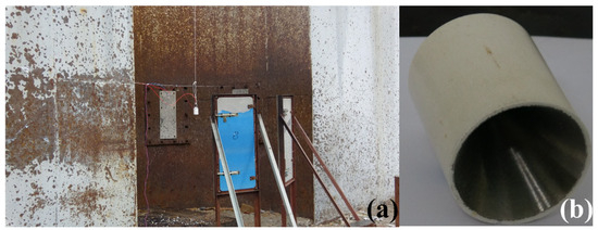
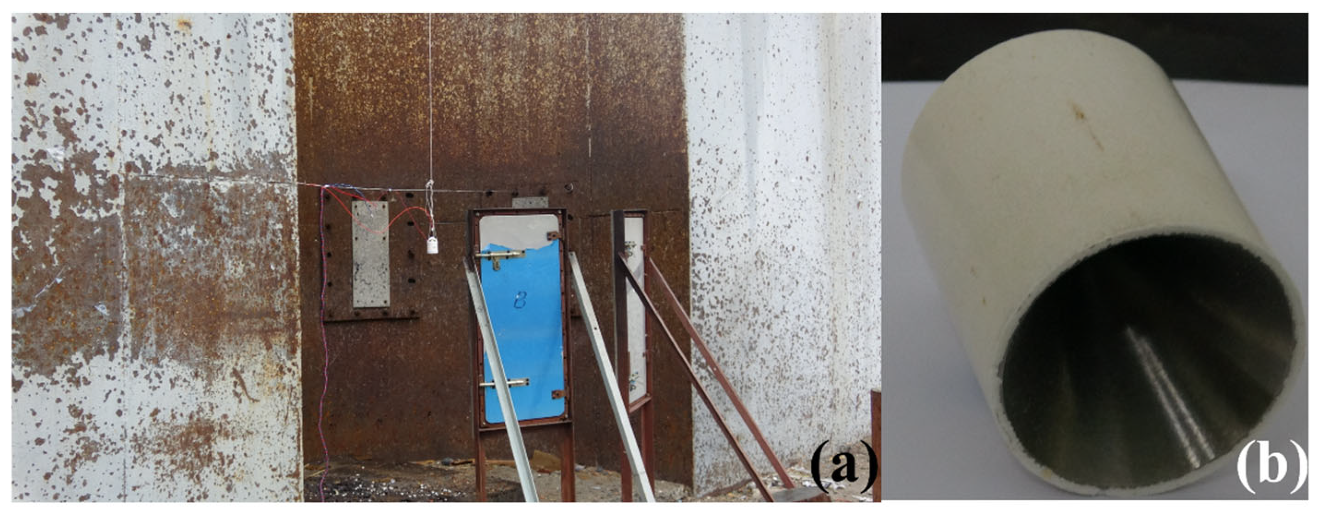
The shape of the jet is an important factor affecting its destructive capability. Therefore, the jet’s shape parameters are obtained from jet formation X-ray experiments to verify the numerical and theoretical results. As shown in Figure 2a, the X-ray equipment includes two X-ray emitters and two film cartridges. The angle between the two radiation emitters is approximately 60°. The shape of the jet at two different time points can be obtained through X-ray generation experiments for subsequent analysis and research. The device takes photos of the jet at two predetermined times, T_A (30 μs) and T_B (50 μs), and then obtains images of the jet’s shape at those times. Based on the jet’s position in the two photos, its velocity can be calculated. The SC is suspended at the central convergence point of the X-rays using fine cotton threads. The diameter of the SC structure used in the experiment is 56 mm, the charge height is 73.3 mm, the cone angle of the charge cover is 60°, and the wall thickness is 1 mm. The explosive used is 8701, with a density of approximately 1.70 g/cm³. The SC adopts the center detonation method of a # 8 electric detonator. The SC structure is shown in Figure 2b.

Figure 2. Jet formation X-ray experimental setup. (a) X-ray experimental setup, (b) SC structure.

2.2. Preparation for Post-Target Jet X-Ray Experiments

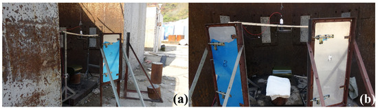
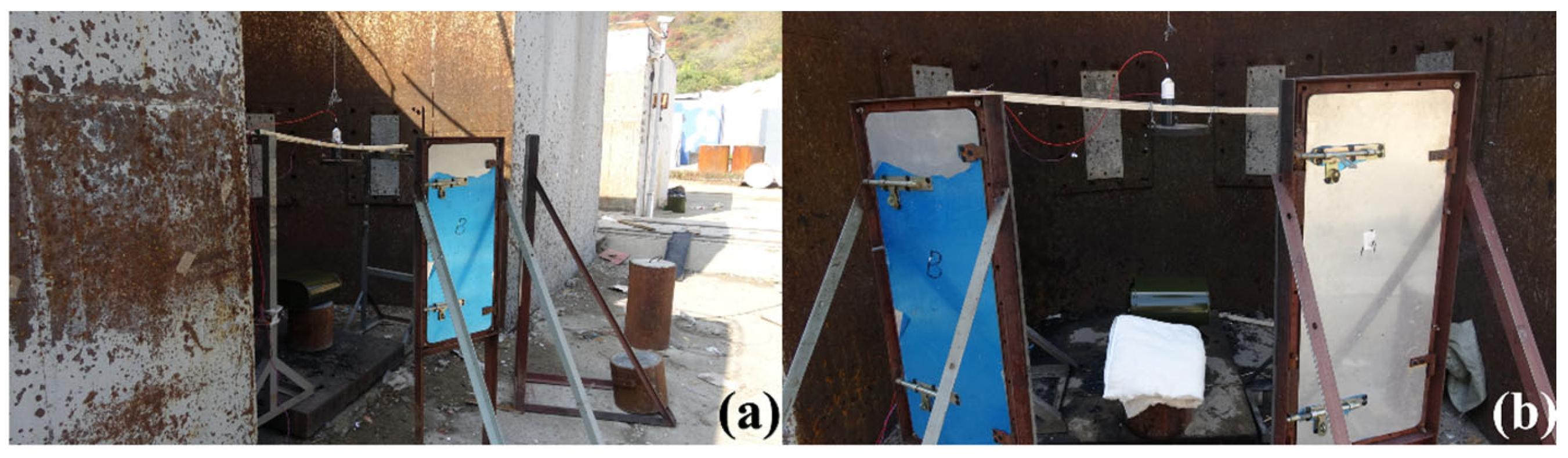
The cohesiveness and the fracture degree of a jet can affect its destructive capability [27,28]. Therefore, the morphological characteristics of the post-target jet are obtained through X-ray experiments. Two wooden sticks about 2 m long are placed on the shelf. A C45 steel target with a diameter of 100 mm and a thickness of 30 mm is fixed to the two wooden sticks using thin wire. Considering that the stretching process of the jet requires a certain amount of time, a 120 mm PVC pipe is placed at the center of the C45 steel target to maintain sufficient stretching of the jet. The position of the C45 steel target is adjusted to ensure that it is level with the ground, as shown in Figure 3. A 30 mm C45 steel target is placed 120 mm below the concentrated charge, and the shooting times T_A (45 μs) and T_B (90 μs) are adjusted to obtain photos of the jet before and after penetrating the target plate. Considering that the penetration ability of Ti₅₅Al₂₀V₅Zr₅Nb₁₅ HEA is weaker than that of a Cu jet, but the active elements such as Ti, Al, and Zr in its composition can enhance the ignition ability of the jet and enhance the composite damage effect of the jet [29,30], oil drums containing kerosene and cotton quilts are placed 1.3 m below the verification target to assess the jet’s ignition capability. Specifically, two different operating conditions are set up for comparison. In the first experiment, only oil drums are placed, and the distance between the oil drums and the SC axis is approximately 80 mm, as shown in Figure 3a. In the second experiment, an additional cotton quilt is placed on the other side of the oil drum at the same horizontal height, with a distance of 140 mm between the cotton quilt and the oil drum, as shown in Figure 3b. Table 1 shows the constant process parameters included in the two experiments.

Figure 3. Post-target X-ray experimental setup: (a) the first experiment; (b) the second experiment.

Table 1. Constant process parameters used in all experiments.

Shaped Charge Geometry				Explosive		Target		Trigger Time
Cone Angle	Thickness	Height	Diameter	Type	Density	Type	Dimensions	TA	TB
60°	1 mm	73.3 mm	56 mm	8701	1.70 g/cm3	C45	100 mm × 30 mm	30 (45) μs	50 (90) μs

2.3. Experimental Results and Analysis

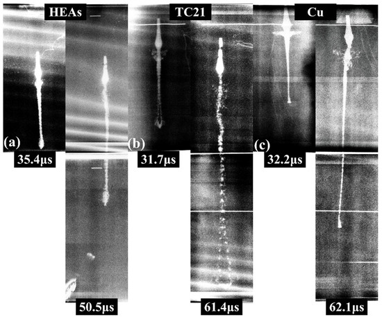
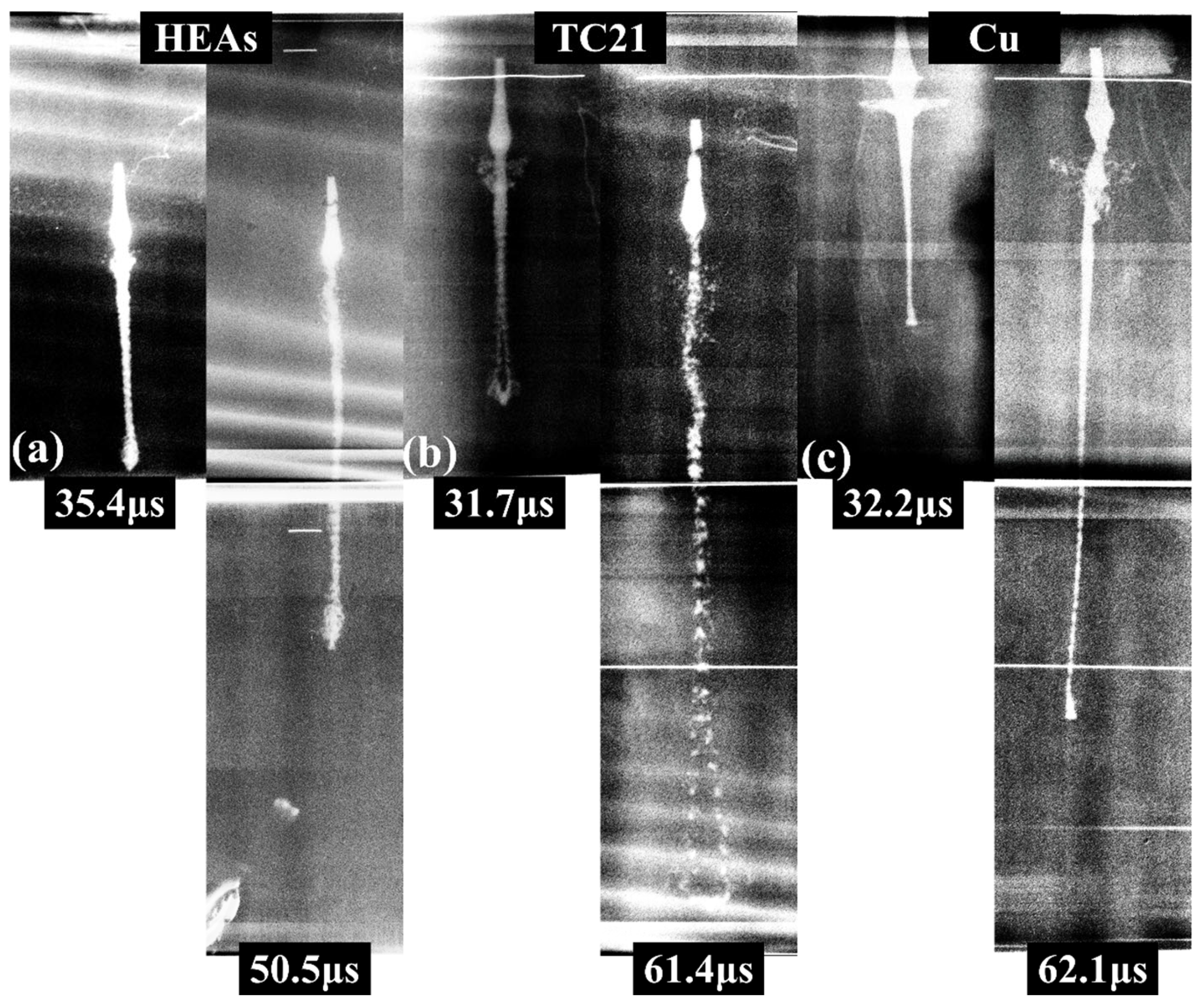
Figure 4 shows the evolution of the jet morphology over time. The jet’s morphology is clearly visible in the photos. In the early stage of jet formation (~30 μs), there are significant differences in the jet morphology, mainly reflected in the head of the jet. For the Cu and Ti₅₅Al₂₀V₅Zr₅Nb₁₅ HEA jets, the head shape is smooth and dense. The head of the TC21 jet shows a clear hollow area, which leads to the maximum degree of fracture of the jet head. In the later stage of jet formation (50–60 μs), there are more significant differences in the morphology of the jet. For the Cu jet, the shape of its head is well maintained, without severe hollowing, and only local fractures occur near the jet head. Compared to the low-density Cu jets, the high-density TC21 and Ti₅₅Al₂₀V₅Zr₅Nb₁₅ HEA jets exhibit poorer cohesiveness. The hollow area of the TC21 jet head is larger, and poor cohesiveness results in the complete disappearance of the jet head shape. In addition, there are significant fractures in the jet from the head to the tail. There are also small and unevenly distributed hollow areas at the head of the Ti₅₅Al₂₀V₅Zr₅Nb₁₅ HEA jet, but most of them are located at the head of the jet. The above phenomenon indicates that under the conditions of this SC structure, the Cu jet exhibits the best cohesiveness, followed by the Ti₅₅Al₂₀V₅Zr₅Nb₁₅ HEA jet, and the TC21 jet exhibits the worst cohesiveness.

Figure 4. Evolution of jet morphology over time: (a) Ti₅₅Al₂₀V₅Zr₅Nb₁₅ HEA; (b) TC21 [31]; (c) Cu [31]. (Reprinted with permission from Ref. [31]. 2022, Elsevier).

Table 2 shows the morphology parameters for three types of jets, including the jet length, the jet diameter, and the jet velocity $V_J$. After calculation, the TC21 jet has the highest velocity (7236 m/s), followed by the Ti₅₅Al₂₀V₅Zr₅Nb₁₅ HEA jet (6982.1 m/s), and the Cu jet (6251 m/s) has the lowest velocity. By comparing the jet diameters, it can be observed that, compared with the initial stage of jet formation, the head diameters of the Ti₅₅Al₂₀V₅Zr₅Nb₁₅ HEA and TC21 jet increased by 37.8% and 54%, respectively, in the final stage of jet formation. This result indicates that for jets with poor cohesiveness (TC21 and Ti₅₅Al₂₀V₅Zr₅Nb₁₅ HEA), radial expansion becomes more pronounced, and the diameter increases over time. For jets with good cohesiveness (Cu), the diameter of the jet head hardly increases.

Table 2. Comparison of jet morphology parameters.

Material	Time	${\mathit{L}}_{\mathit{J}}$/(mm)	${\mathit{D}}_{\mathit{j}}$/(mm)	${\mathit{V}}_{\mathit{J}}$/(m/s)	${\mathit{V}}_{\mathit{J}}^{\mathit{PER}}$/(m/s)	Error/%
Ti55Al20V5Zr5Nb15	35.4 μs	111.3	7.98	6982.1	7665	9.8
	50.5 μs	209.1	11.0
TC21	31.7 μs	111.3	15.9	7236	7691	6.3
	61.4 μs	290.1	24.5
Cu	32.2 μs	105.1	6.3	6251	7155	14.5
	62.1 μs	256.9	5.9

Table 2 also compares the PER model’s calculation results $V_J^{PER}$. The maximum error for the PER model is 14.5% (Cu), and the minimum is 6.3% (TC21). The reason for this phenomenon is that the PER model overestimates the effective pressure used for the unloading acceleration in the shock pressure, resulting in significantly higher calculation results.

2.3.1. Evolution Process of Post-Target Jet Morphology

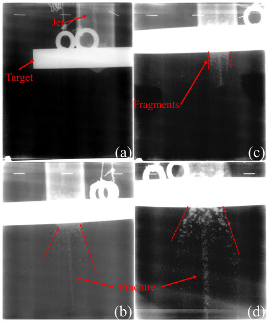
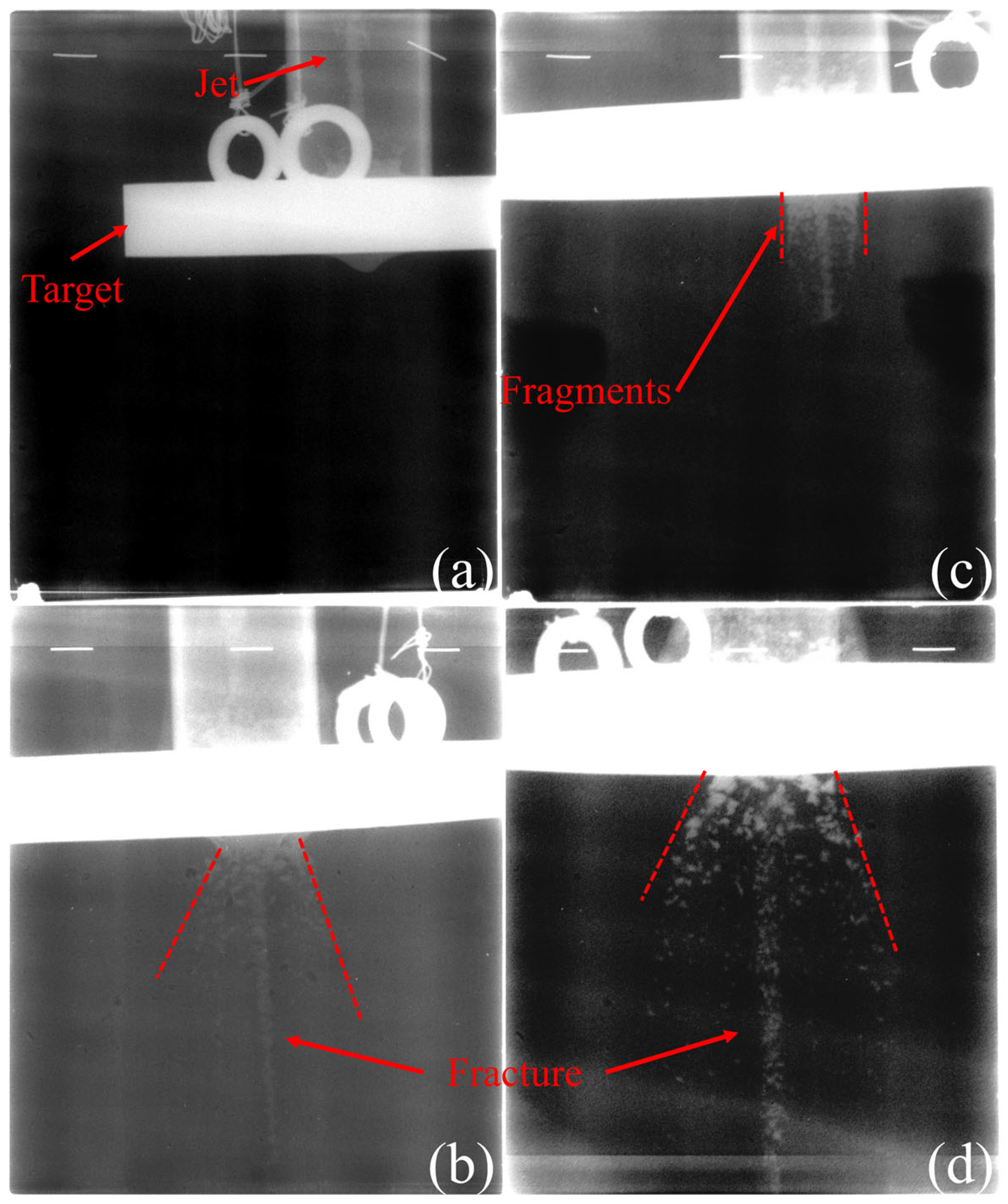
Figure 5 shows the evolution process of the post-target jet in two experiments. Figure 5a,b show the results of the first experiment. At 44.7 μs, the jet is penetrating the C45 steel target, and there are obvious protrusions on the back of the C45 steel target. At 74.8 μs, the jet completely penetrates the target and continues to stretch in the air. Figure 5c,d show the results of the first experiment. At 54.7 μs, the jet penetrates the C45 steel target, and the jet head is completely consumed. At 99.7 μs, the jet completely penetrates the target. In addition, after penetrating the target, the jet is accompanied by large-sized fragments flying towards the outer area of the jet, which come from the collapsed fragments on the back of the C45 steel target. In Figure 5b–d, it can be observed that in both of the experiments, the jet shows obvious fracture characteristics after penetrating the target, mainly manifesting as discrete “particle clusters”. Its characteristic is the significant spacing and void between the particles. This unique phenomenon is also observed in the TC21 and TB6 jets [31]. When there are gaps between the particles, external airflow can enter the gaps, resulting in a significant pressure gradient around the particles. The pressure gradient generates an asymmetric load distribution on the particle surface, which in turn induces a deflection torque. Under this torque, the particle undergoes a spatial attitude reversal, causing its penetration direction to deviate from the original flight axis, thereby significantly reducing the jet’s overall penetration efficiency. Although the continuity between the particles is poor, the particles do not move radially but follow the preceding particle clusters along the axial direction. This phenomenon indicates that the Ti₅₅Al₂₀V₅Zr₅Nb₁₅ HEA jet behind the target has good collimation.

Figure 5. Ti₅₅Al₂₀V₅Zr₅Nb₁₅ HEA post-target jet morphology: (a) 44.7 μs; (b) 74.8 μs; (c) 54.7 μs; (d) 99.7 μs.

The above phenomenon indicates that significant fracture characteristics are the primary factor limiting the jet penetration capability of Ti₅₅Al₂₀V₅Zr₅Nb₁₅ HEA, but their good collimation ensures the jet’s destructive capability under high-standoff conditions.

Regarding generalizability, it is instructive to consider how the trends might change for HEA with different mechanical properties. For Ti₅₅Al₂₀V₅Zr₅Nb₁₅ HEA with a BCC structure, the higher strength may lead to a decrease in jet velocity [8]. Due to the low ductility of the material, the jet exhibits poorer cohesiveness during the formation process. For high-strength HEA, their ductility is often poor. Therefore, the jets have poorer cohesiveness and are more prone to fracture and radial expansion during the formation process. However, this significant feature also promotes the hole-expanding effect of the jet on the target.

2.3.2. Analysis of Damage Efficiency

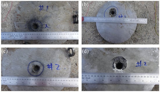
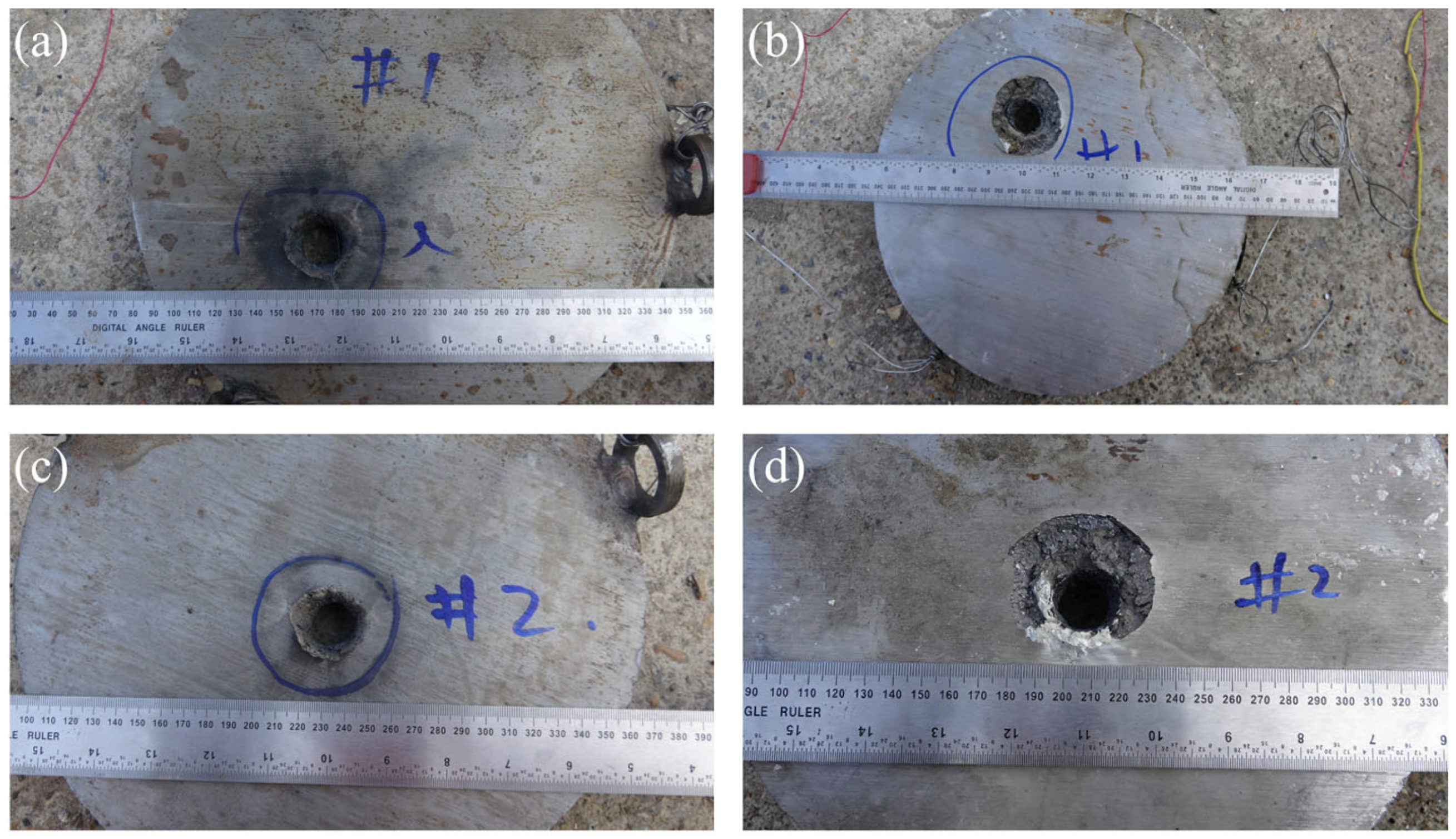
Figure 6 shows the damage to the C45 steel target in two experiments. As shown in Table 3, in the first experiment, the diameter of the entry hole $D_1$ on the validation target is about 36 mm, the diameter of the exit hole $D_2$ is about 25 mm, and the diameter of the collapse area $D_3$ on the back is about 51 mm. In the second experiment, $D_1$, $D_2$ and $D_3$ are 34 mm, 26 mm, and 53 mm. In addition, there is only one obvious and clear through-hole on the front of the two targets, and no other holes are seen, indicating that the Ti₅₅Al₂₀V₅Zr₅Nb₁₅ HEA jet has a good jet shape before entering the target and does not exhibit dispersion. Compared to the Cu jet (32 mm) [31], the Ti₅₅Al₂₀V₅Zr₅Nb₁₅ HEA jet has a larger opening diameter, corresponding to an increase of about 12.5%. Although it does not have excellent penetration capability, its efficient hole-expanding ability is also a concern for scholars.

Figure 6. Damage to the C45 steel target: (a) front of the # 1 target; (b) back of the # 1 target; (c) front of the # 2 target; (d) back of the # 2 target.

Table 3. Penetration aperture statistics.

Experiment	D1/mm	D2/mm	D3/mm
1	36	25	51
2	34	26	53

The X-ray radiographs reveal that the jet breaks up into discrete “particle clusters” after penetrating the C45 steel target. This phenomenon indirectly proves that Ti₅₅Al₂₀V₅Zr₅Nb₁₅ HEA jets have already fractured before penetration. However, in the early stage of the jet stretching process, the spacing between the particle clusters is small and difficult to observe in the photo. The discrete particle clusters expand their holes through repeated impacts during penetration, and good collimation maintains the concentration of the penetration direction. However, the gaps between the clusters result in energy interruption during the penetration process, reducing the penetration efficiency of the jet. Especially under high-standoff conditions, the penetration depth of the fractured jet significantly decreases [27,31].

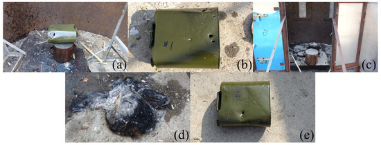
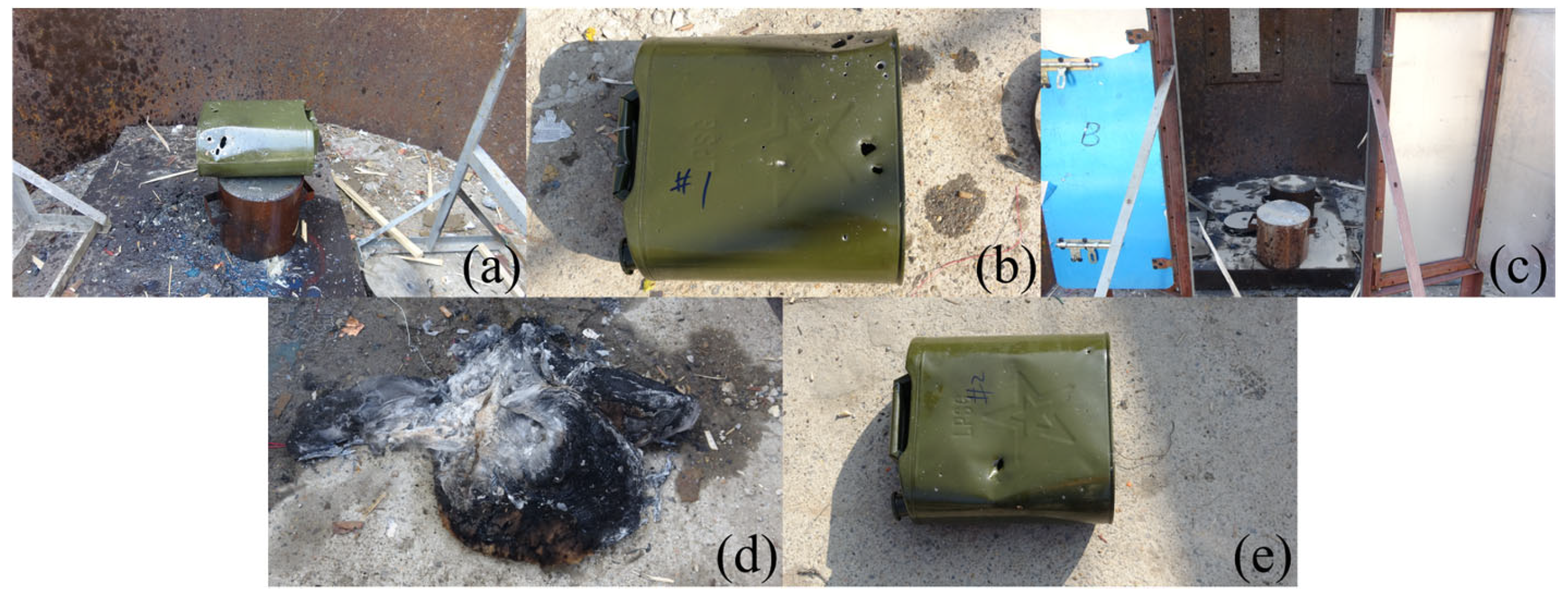
To prevent kerosene leakage from affecting the results of the second experiment, fine sand is used to cover the ground at the experimental site, and the second experiment is conducted according to the experiment setup shown in Figure 7c. Figure 7d,e show the damage to the cotton quilt and oil drum in the second experiment. The damage mode of the oil drum in this experiment is essentially the same as in the first experiment. There are local depressions and large deformations on the front of the oil drum, along with a significant perforation and several small perforations. The cotton quilt that fell to the ground under the impact shows obvious burn marks.

Figure 7. The damage of combustion: (a) side of oil drum # 1; (b) front of oil drum # 1; (c) experiment site correction; (d) cotton quilt # 2; (e) front of oil drum # 2.

Based on the results of the two experiments, it can be inferred that the oil drum and the cotton quilt are located at radial offsets of 80 mm and 60 mm from the penetration axis, respectively, and that the post-target jet does not come into contact with the combustible. Therefore, neither of them is directly ignited by the jet. The damage mechanism primarily results from the combined impact of target fragments and residual fragments from the jet, causing penetrating damage to the oil drum and subsequent internal kerosene leakage. Due to its light weight and its proximity to the penetration axis, the cotton quilt is displaced and falls to the ground upon impact. As time passes, heat transfer continues, and the cotton quilt is eventually ignited by high-temperature jet fragments, initiating combustion. This process indicates that although the jet does not directly act on the cotton quilt, the accompanying high-temperature fragments can still serve as an ignition source, triggering secondary combustion under certain heat-transfer conditions.

3. Numerical Computation-Assisted Research

Two jet morphology photos can be obtained from the X-ray formation experiments, but more characteristic parameters of the jet cannot be obtained. Therefore, obtaining additional characteristic parameters of the jet using high-fidelity numerical methods supports the theoretical calculations. At the same time, verifying the numerical calculations against the experimental results can improve their credibility.

3.1. Finite Element Model and Data Extraction Method

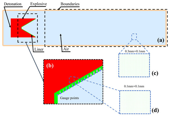
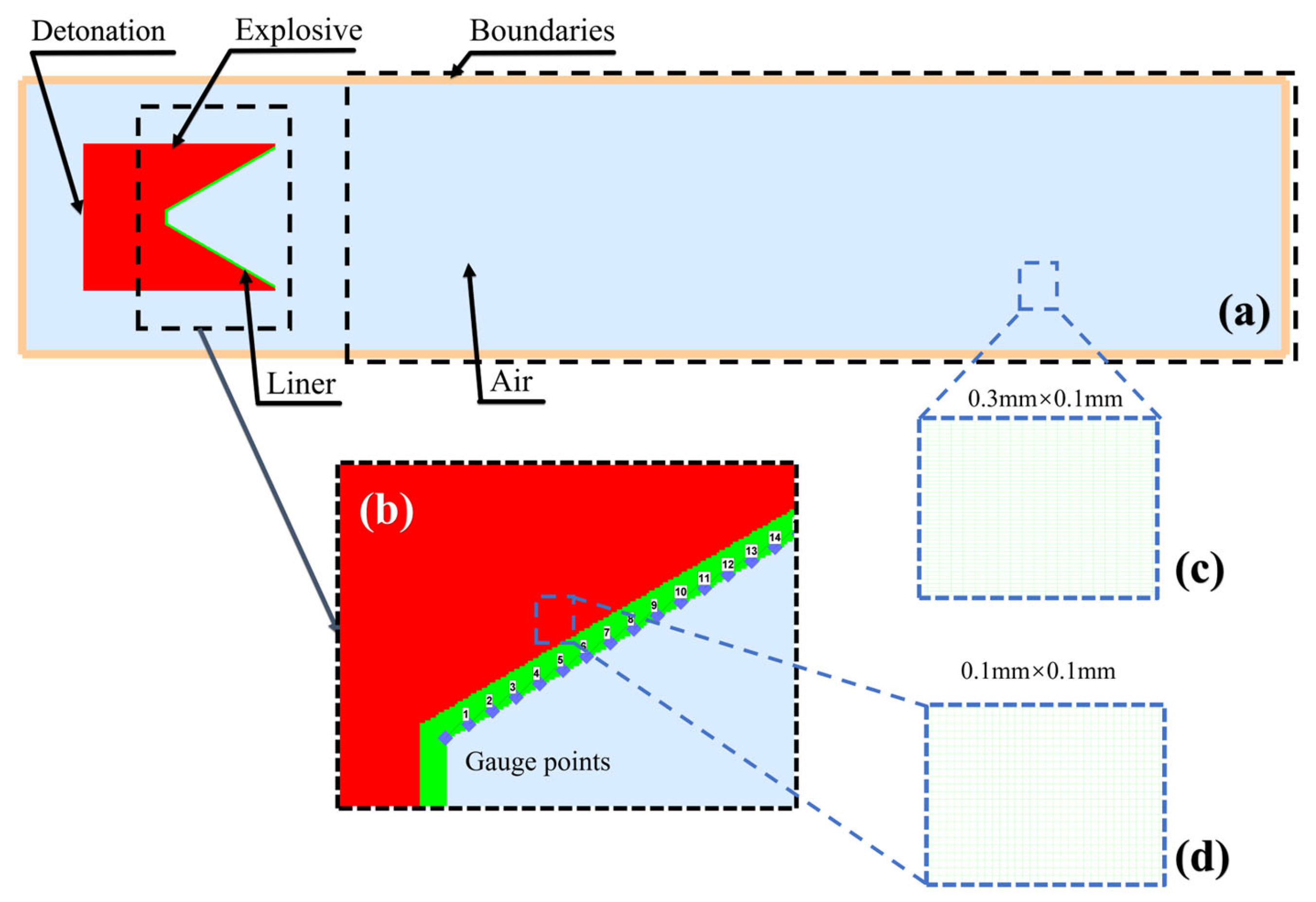
Numerical simulation is an efficient method for studying the collapse and jet formation of SCJs. Therefore, based on the actual structure of the SC, this article examines the performance of SCJs and establishes a 2D axisymmetric model, as shown in Figure 8a. The model includes explosives, air, and liner, all of which use the Euler method. The model boundary is specified as outflow. The detonation point is established at the center of the explosive endpoint.

Figure 8. Finite element model: (a) calculation model; (b) Gauge point distribution; (c) grid size of jet channel; (d) grid size of liner.

Specifically, in order to study the dynamic response characteristics of the elements of the liner at the collision regime, 48 Gaussian points are established at equal intervals on the outer side of the liner, as shown in Figure 8b. Gaussian points can be used to monitor material state and extract key parameters for the theoretical models, such as pressure, temperature, stress, and velocity.

The entire computational domain area is approximately 480.3 mm × 104 mm. As shown in Figure 8c, the grid size for the jet channel on the right side of the model is 0.3 mm × 0.1 mm. As shown in Figure 8d, to ensure computational accuracy and save time, the grid size for both the explosive and the liner is 0.1 mm × 0.1 mm. For the air domain on the left and above the model, a 0.3 mm gradient grid is used, as shown in the Figure.

3.2. Material Model and Parameter Determination

The SC uses 8701 explosive, and the Jones–Wilkins–Lee (JWL) EOS can be expressed as follows [32]:

$$P_e=A_e(1-{\displaystyle \frac{\omega }{R_1{V}_e}})e^{-R_1{V}_e}+B_e(1-{\displaystyle \frac{\omega }{R_2{V}_e}})e^{-R_2{V}_e}+{\displaystyle \frac{\omega E_e}{V_e}}$$

(1)

where $P_e$ is the pressure; ${\rho }_e$ is the density of explosive; $V_e=1/{\rho }_e$ is the relative volume; and $E_e$ is the internal energy per unit mass of explosive.

The remaining parameters are constants obtained through experiments and fitting, as shown in Table 4.

Table 4. Parameters of 8701 explosive.

ρe/(g/cm)	A/GPa	B/GPa	R1	R2	ω	De/(m/s)	PCJ/GPa
1.702	618.4	6.9	4.3	0.87	0.38	8350	29.66

The ideal gas EOS is used to describe air:

$$P_{air}=(\gamma -1){\rho }_{air}{E}_{air}$$

(2)

where ${\rho }_{air}$ is the density of air; $E_{air}$ is the internal energy per unit mass of air; and $\gamma$ is a constant of 1.4.

The Johnson–Cook (J–C) model, as a commonly used strength model for metal materials, can be applied to describe the flow stress of materials at high strain rates and high temperatures. The basic form of the J–C model is written as follows [33]:

$${\sigma }_y=\left(A+B{\epsilon }_p^n\right)\left(1+C\ln {\dot{\epsilon }}_p\right)\left(1-T^{*m}\right)$$

(3)

where ${\sigma }_y$ is the Von Mises equivalent stress; ${\epsilon }_p$ is the equivalent plastic deformation; ${\dot{\epsilon }}_p=\dot{\epsilon }/{\dot{\epsilon }}_0$ is the normalized effective plastic strain rate; ${\dot{\epsilon }}_0$ is the reference strain rate; $A$ is the initial yield strength; $B$ is the hardening modulus; $n$ is the stress hardening exponent; $C$ is the strain rate hardening coefficient; $m$ is the thermal softening coefficient; $T^{*}=\left(T-T_{ref}\right)/\left(T_{melt}-T_{ref}\right)$ is the relative temperature; $T$ is the current temperature; $T_{melt}$ is the melting temperature; and $T_{ref}$ is the reference temperature. Table 5 shows the J–C model parameters for the three types of liner materials.

Table 5. J–C model parameters for liner materials.

Material	A/MPa	B/MPa	n	C	m	Tmelt/K
Ti55Al20V5Zr5Nb15 [8]	965	450	0.97	0.0215	0.60	1943
TC21 [34]	1030	1680	0.69	0.018	1.40	1935
Cu [35]	90	292	0.31	0.025	1.09	1356

The liner materials adopt the Mie–Grüneisen EOS:

$$p=p_H+{\displaystyle \frac{\Gamma }{v}}(e-e_H)$$

(4)

where $p$ is the pressure; $e$ is the energy; $p_H$ is the Hugoniot pressure; $e_H$ is the Hugoniot energy; $\Gamma$ is the Grüneisen coefficient; and $v=1/\rho$ is the specific volume. Table 6 shows the EOS parameters of the materials.

Table 6. EOS parameters of materials.

Material	C0/(m/s)	S	Γ0
Ti55Al20V5Zr5Nb15 [8]	0.5026	1.01	1.33
Cu	0.3940	1.489	2.02
TC21	0.5110	1.338	1.23

3.3. Numerical Calculation Results and Analysis

3.3.1. Evolution Process of Jet Morphology

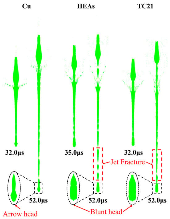
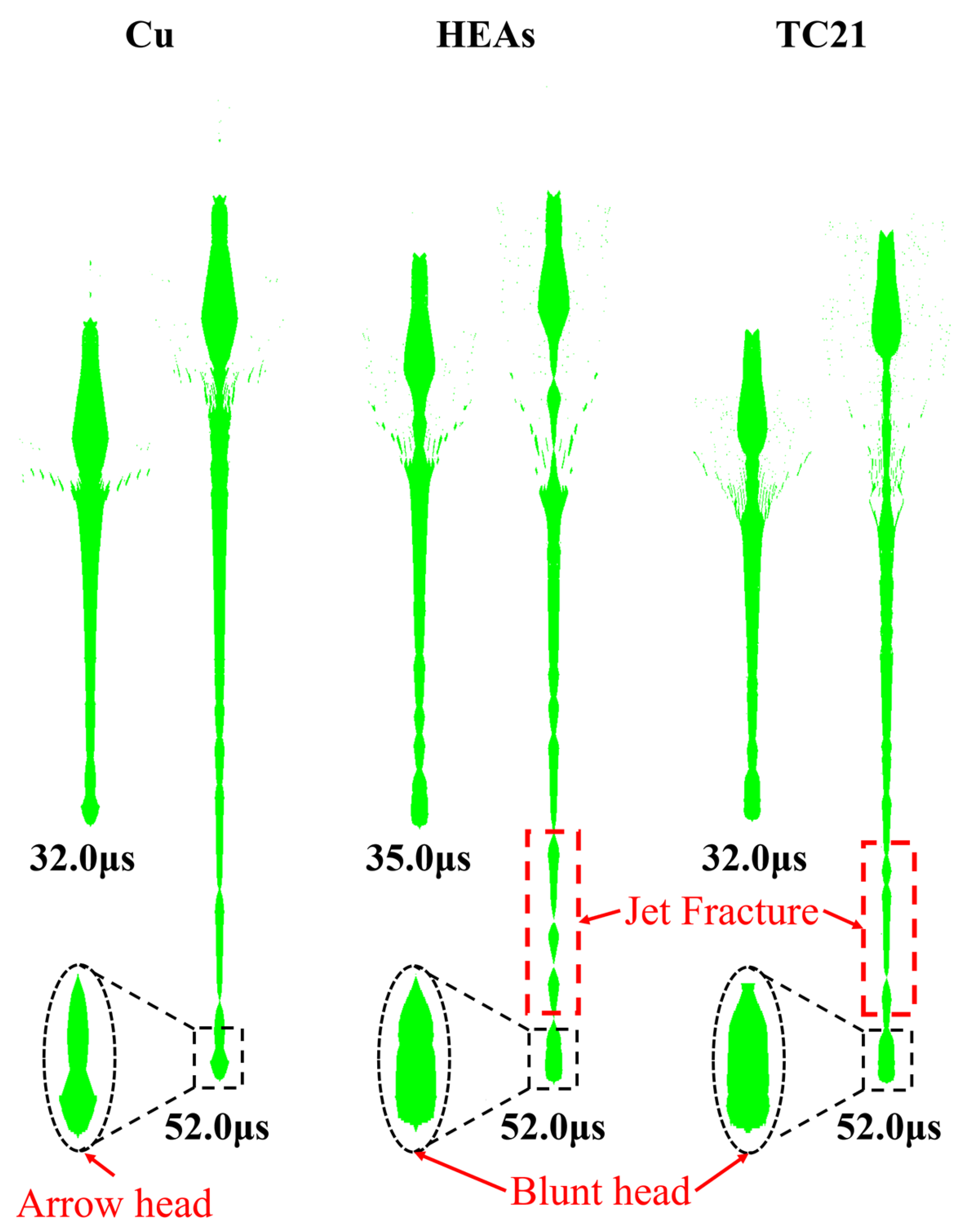
The numerical calculation results of jet formation are shown in Figure 9. Overall, there are significant differences in the morphology of the three types of jets. In the early stage of jet formation (~30 μs), there are varying degrees of accumulation at the jet head, caused by the short acceleration time and the low velocity of the material at the top of the liner, resulting in accumulation due to the subsequent high-velocity impact. As time increases, the jet exhibits varying degrees of tensile fracture. The fracture degree of the Ti₅₅Al₂₀V₅Zr₅Nb₁₅ HEA jet is more severe, and the continuity of the Cu jet is the best.

Figure 9. Comparison of results of jet head morphology analysis.

The morphology of the jet head can indirectly reflect its cohesiveness: the “arrow” shape typically indicates jets with good cohesiveness, whereas the “blunt head” shape indicates jets with poor cohesiveness [31]. Although a larger grid aspect ratio is used in the numerical calculations in this article, a precise simulation of the jet head morphology is still achieved. As shown in the partially enlarged image in Figure 9, the Cu jet head is slender and protruding, indicated by clear arrows. The heads of the Ti₅₅Al₂₀V₅Zr₅Nb₁₅ HEA jet and the TC21 jet are flat and noticeably blunt. This result further indicates that the cohesiveness of the TC21 and Ti₅₅Al₂₀V₅Zr₅Nb₁₅ HEA jets is poor.

Table 7 summarizes the relevant numerical calculation results, with the relative error between the numerical simulation and experimental results in parentheses. The maximum error in jet length is +4.58%, and the maximum error in jet velocity is −2.12%, with all errors not exceeding 5%. These results indicate that the numerical model established in this paper can well simulate the jet formation process of Cu, TC21, and Ti₅₅Al₂₀V₅Zr₅Nb₁₅ HEA materials, verifying the effectiveness and reliability of the numerical calculation model in predicting jet morphology.

Table 7. Comparison between numerical calculation and experimental results.

Material	Time	Jet Length/(mm)	VJ/(m/s)
Ti55Al20V5Zr5Nb15 [8]	35.0 μs	116.4 (+4.58%)	7091 (+1.56%)
	52.0 μs	207.8 (−0.6%)
TC21 [31]	32.0 μs	108.1 (−2.88)	7082 (−2.12%)
	52.0 μs	234.2
Cu [31]	32.0 μs	102.9 (−2.09%)	6253 (+0.03%)
	52.0 μs	205.2

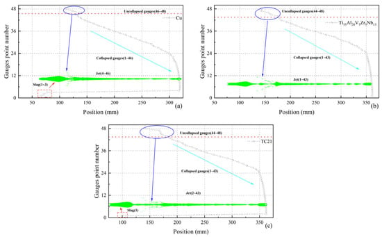
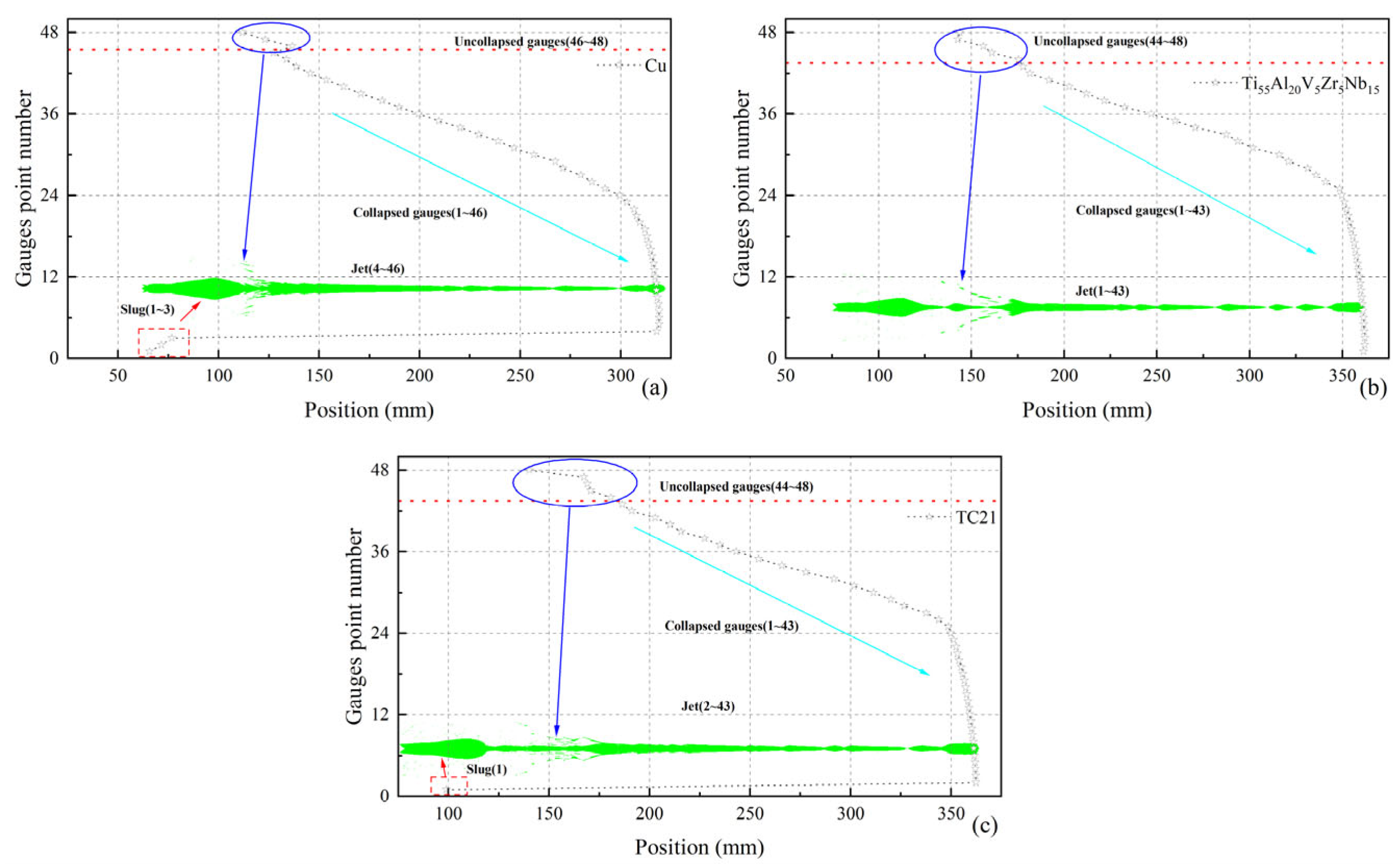
Figure 10 shows the distribution characteristics of the Gauge points in the three different material jets. As shown in Figure 10a, the calculation results for the Cu jet indicate that about 46 Gauge points are collapsed, with 3 located in the slug and the rest distributed in the jet. Only three Gauge points remained uncollapsed. Figure 10b shows the calculation results of the Ti₅₅Al₂₀V₅Zr₅Nb₁₅ HEA jet. Approximately 43 Gauges points are collapsed, all located in the jet section, but there are still 5 Gaussian points that are not collapsed. Figure 10c shows the calculation results of the TC21 jet, with approximately 43 Gauge points collapsed, including 1 Gaussian point located in the slug, but 5 Gauges points not collapsed. It is worth noting that due to the high density of the Cu jet, its collapse velocity is relatively low, making it difficult for the Gauge point located at the top of the liner to form a jet. In contrast, in the bottom area of the liner, the TC21 and Ti₅₅Al₂₀V₅Zr₅Nb₁₅ HEA jets have more Gauge points that have not been collapsed, indicating that the effective mass proportion in the TC21 and Ti₅₅Al₂₀V₅Zr₅Nb₁₅ HEA jets is relatively small, and the jet mass that effectively participates in the subsequent penetration process is relatively low. This phenomenon further affects the jet’s axial penetration, providing a key numerical basis for understanding the differences in jet formation performance and penetration efficiency among the materials.

Figure 10. Gauge point position distribution: (a) Cu; (b) Ti₅₅Al₂₀V₅Zr₅Nb₁₅ HEA; (c) TC21.

3.3.2. Analysis of the Typical Liner Element Collapse Process

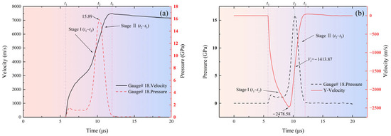
Figure 11a shows the pressure and velocity evolution curves over time for a typical element (Gauge # 18). The collapse process of a typical element is mainly divided into two characteristic stages: stage I and stage II. In stage I (t₁~t₂), the element begins to collapse and move towards the axis of symmetry, entering the shock-loading stage. At this point, the pressure rapidly rises to its peak (15.89 GPa), while the element gains significant velocity, marking the beginning of kinetic energy accumulation. In stage II (t₂~t₃), the element leaves the compression stage and enters the unloading stage. The pressure rapidly decays from its peak to zero, while the velocity continues to increase, indicating that kinetic energy continues to grow as potential energy is converted to kinetic energy. This phenomenon further confirms the contribution of the unloading stage to the increase in jet velocity. After stage II, the jet begins to stretch, and the element detaches from the liner’s main body. The pressure only shows slight fluctuations, while the velocity gradually decreases due to viscous dissipation and geometric stretching.

Figure 11. Typical liner element collapse process: (a) evolution curves of pressure and velocity over time; (b) evolution curves of normal velocity and pressure over time.

The numerical calculations indicate that a typical element undergoes two key stages, compression and unloading, during the collapse process, and that the velocity shows an upward trend in both stages. The compression stage is characterized by a significant pressure peak and is the core stage for energy input and momentum transfer. The simulation results clearly reveal the core physical process of “shock-compression unloading.” During the compression phase, the pressure reaches its peak, achieving material compression and initial acceleration. During the unloading stage, the pressure energy is converted into kinetic energy, further increasing the jet velocity. During the compression stage, the element velocity increases from 0 to 5653.88 m/s. During the unloading stage, the element velocity increases to a peak of 7496.28 m/s. The compression and unloading stages contribute 75.42% and 24.58% to the increase in velocity, respectively. This result further validates the unloading acceleration phenomenon in the theoretical model.

Figure 11b shows the evolution curves of pressure and normal velocity over time for a typical element (Gauge # 18). During stage I (t₁~t₂), the normal velocity of a typical element rapidly increases to its maximum value (−2478.58 m/s), while the element pressure is still rising. When the element pressure reaches its peak, the normal velocity begins to decrease, and the corresponding value is −1413.87 m/s, which can be regarded as the element’s cutoff velocity. Afterward, the element pressure gradually decays to zero, in phase with the normal velocity. This behavior indicates that the peak of the element’s normal velocity lags behind the peak of the pressure, resulting in only a portion of the normal momentum being converted into impact momentum.

4. Theory Model

The experimental results indicate that the predictions of the traditional models are significantly higher. Therefore, this Section establishes an enhanced theory of jet formation. The impact compression and isentropic unloading state parameters, as well as the jet velocity of the materials, are solved using theoretical models. In addition, based on the J–C model, the Newton iteration method is used to solve for the dynamic yield strength.

4.1. Basic Assumptions and Physical Models

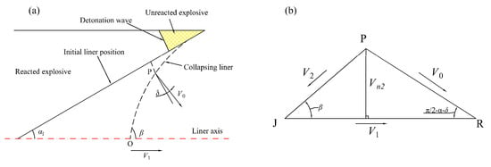
Because the SC is completely axisymmetric, a two-dimensional symmetric model is established in this paper for the jet formation process, as shown in Figure 12a. To construct a solvable analytical model, the jet formation process is decomposed into two sequential, quasi-one-dimensional stages:

Figure 12. Model of liner collapse: (a) collapse process of liner; (b) geometric relationship between V₂, V_n2 and V₀.

Collision and Compression (Stage I): The elements of the liner are along the axis of symmetry, with the velocity and the angle relative to the axis as the motion proceeds. In the collision-point reference frame, this process is treated as a steady oblique shock-wave problem. At this stage, the research objects are the liner elements without thickness.

Stretching and Unloading (Stage II): The jet formed after the collision moves outward from the collision point undergoes isentropic unloading, restoring the density to ${\rho }_0$ while obtaining axial acceleration. At this stage, the research objects are the jet elements formed after the collision, whose paths coincide with the axis of symmetry.

To ensure that the model can be analytically solved while maintaining its physical essence, the following assumptions are introduced in this paper:

• In the collision-point reference frame, the flow is steady. This means the geometric relationship between flow and collapse velocities is constant, as shown in Figure 11b.
• The actual non-stationary collision process, characterized by the particle velocity $u_p$, shows that the shock wave intensity varies over time. To characterize its overall effect in the analytical model, we introduce an equivalent average particle velocity ${\overline{u}}_p$ to replace the constant value $u_p$ in the steady-state model.
• After compression, the unloading and expansion process of the jet elements is approximately an isentropic process.
• The path of the jet elements unloading from the compression state to the final state is described by the isentropic lines of the material on the $\left(p-v\right)$ plane. It is assumed that the unloading endpoint density ${\rho }_{\mathit{f}}$ returns to the initial density ${\rho }_0$ of the material, but the temperature and pressure are different from the initial values.

4.2. Impact Compression and Momentum Conversion Mechanism

4.2.1. Dynamic Momentum Conversion Factor Based on Mach Number Calibration

The PER theory assumes that collision is a steady-state process [26], in which the particle velocity equals the incoming velocity $V_2$. However, in reality, collision is a transient pulse process: at the initial moment of collision, the material collides at a normal velocity $V_{\mathit{n}2}$. Due to the reverse pressure gradient generated by the impact compression and the resistance of the material’s own strength, the normal velocity rapidly decays. Therefore, the effective particle velocity that characterizes the impact strength is not the initial value, $V_{\mathit{n}2}$, but the average effect of its decay over time.

To describe this, we introduce the equivalent average particle velocity ${\overline{u}}_p$. Its physical basis is that, in the collision-point reference frame, the net impulse on the material element equals the change in its momentum. The impulse is determined by two competing factors: the compression impulse, driven by the flow pressure, and the resistance impulse, caused by the material’s wave impedance. To quantify this competition, we define the impact Mach number $\mathit{Ma}$:

$$Ma={\displaystyle \frac{V_{n2}}{C_0}}$$

(5)

where $Ma$ directly characterizes the intensity of the material’s impact. The larger the value of $Ma$, the greater the impact velocity, and the material’s dynamic response tends to be more fluid.

Based on dimensional analysis and physical reasoning, ${\overline{u}}_p$ should be related to $V_{\mathit{n}2}$ and $Ma$. ${\overline{u}}_p$ satisfies the following function form:

$${\overline{u}}_p=V_{\mathit{n}2}\cdot f\left(Ma\right)$$

(6)

where $f\left(Ma\right)$ should satisfy the following boundary conditions:

• When $Ma\to 0$, the material is in a quasi-static condition, $f\left(Ma\right)\to 0$, ${\overline{u}}_p\to 0$;
• When $Ma\to \infty$, the collision approximates an ideal fluid impact, $f\left(Ma\right)\to {\displaystyle \frac{1}{2}}$, ${\overline{u}}_p\to {\displaystyle \frac{V_{\mathit{n}2}}{2}}$.

A logistic function that satisfies the above boundary conditions and has a concise form:

$$f\left(Ma\right)={\displaystyle \frac{0.5}{1+e^{-k\left(Ma-M{a}_0\right)}}}$$

(7)

where $k$ and $M{a}_0$ are the material parameters related to the dynamic yield strength of the material.

We define the momentum conversion efficiency factor $\left({\prod }_{DMCF}\right)$ as the ratio of the actual impact momentum ${\rho }_0{\overline{u}}_p$ to the maximum impact momentum ${\rho }_0{V}_{\mathit{n}2}$:

$${\prod }_{DMCF}={\displaystyle \frac{{\rho }_0{\overline{u}}_p}{{\rho }_0{V}_{\mathit{n}2}}}={\displaystyle \frac{{\overline{u}}_p}{V_{\mathit{n}2}}}$$

(8)

Then, ${\prod }_{DMCF}$ can be expressed as follows:

$${\prod }_{DMCF}=2f\left(Ma\right)$$

(9)

In the actual impact process, $u_p$ rapidly decays from $V_{\mathit{n}2}$ to $V_r$. Using a linear decay model for approximation, ${\overline{u}}_p$ is calculated as follows:

$${\overline{u}}_p={\displaystyle \frac{1}{2}}(V_{n2}-V_r)$$

(10)

Equation (10) can be rewritten as follows:

$${\overline{u}}_p={\displaystyle \frac{1}{2}}{V}_{n2}(1-{\displaystyle \frac{V_r}{V_{n2}}})$$

(11)

Combining Equations (6) and (11) gives the following Equation (12):

$${\prod }_{DMCF}=1-{\displaystyle \frac{V_r}{V_{n2}}}$$

(12)

Then, ${\overline{u}}_p$ can be expressed as follows:

$${\overline{u}}_p={\displaystyle \frac{V_{\mathit{n}2}}{2}}\cdot {\prod }_{DMCF}={\displaystyle \frac{V_{\mathit{n}2}}{2}}\cdot {\displaystyle \frac{1}{1+e^{-k\left(Ma-M{a}_0\right)}}}$$

(13)

According to Equation (13), ${\prod }_{DMCF}$ is a function of $Ma$ with a value range of $\left(0,1\right)$. When $Ma\ll M{a}_0$, ${\prod }_{DMCF}\to 0$. When $Ma=M{a}_0$, ${\prod }_{DMCF}=0.5$. When $Ma\gg M{a}_0$, ${\prod }_{DMCF}\to 1$. ${\prod }_{DMCF}$ also characterizes the proportion of the shock pressure used for unloading acceleration. The higher the value of ${\prod }_{DMCF}$, the higher the proportion of unloading acceleration.

$\mathit{k}$ is the growth rate coefficient that characterizes the transition of the materials from “strength dominant” to “kinetic dominant”. A larger value of $\mathit{k}$ indicates a rapid increase in momentum conversion efficiency within a narrow range of $Ma$.

$M{a}_0$ is the half-efficiency point. It characterizes the material’s “strength threshold”. High-dynamic-strength materials require a higher $Ma$ (i.e., more intense collisions) to achieve the same momentum-conversion efficiency; therefore, their $M{a}_0$ value is higher.

4.2.2. Solution of Shock-State Parameters

When ${\overline{u}}_p$ is given, the state of the shock wave front can be determined by combining the conservation equations for mass and momentum with the material EOS.

For the wave velocity D, the fitted linear relationship between the shock wave velocity D and ${\overline{u}}_p$ is as follows [36]:

$$D=C_0+S{\overline{u}}_p$$

(14)

where $C_0$ is the initial sound velocity of the material; $S$ is constant.

According to the mass conservation equation, the density ratio before and after the shock wave front is as follows:

$${\displaystyle \frac{{\rho }_1}{{\rho }_0}}={\displaystyle \frac{D}{D-{\overline{u}}_p}}$$

(15)

If the volume ratio is defined as $\eta =1-v_0/v_1=1-{\rho }_0/{\rho }_1$, then $\eta ={\overline{u}}_p/D$.

According to the momentum conservation equation, the shock pressure $p_s$ can be expressed as follows:

$$p_s={\rho }_{0}D{\overline{u}}_p$$

(16)

According to the energy conservation equation, the increment of specific internal energy after impact is as follows:

$$e_1={\displaystyle \frac{1}{2}}{p}_s\left(v_0-v_1\right)={\displaystyle \frac{p_s\eta }{2{\rho }_0}}$$

(17)

where $v_0=1/{\rho }_0$ and $v_1=1/{\rho }_1$.

The Hugoniot pressure $p_H$ and energy $e_H$ can be expressed as a function of the volume ratio η:

$$p_H\left(\eta \right)={\displaystyle \frac{{\rho }_0{C}_0^2\eta }{{\left(1-S\eta \right)}^2}},e_H\left(\eta \right)={\displaystyle \frac{p_H\eta }{2{\rho }_0}}$$

(18)

Assuming that the internal energy increment is fully converted into thermal energy, the impact temperature $T_1$ is as follows:

$$T_1=T_{ref}+{\displaystyle \frac{e_1}{Cv}}$$

(19)

where $Cv$ is the specific heat capacity.

4.3. Unloading Velocity Parameter Solving Method Based on Grüneisen EOS

When the material is isentropically unloaded from the compression state to the final state $\left({\rho }_f={\rho }_0,p_f\approx 0\right)$, the velocity increment a of the particles $\Delta u$ can be expressed as follows [37]:

$$\Delta u={\int }_0^{p_H}\sqrt{-{(\partial V/\partial P)}_{\mathrm{s}}}\mathrm{d}P$$

(20)

where the subscript S represents the trajectory integral along the isentropic unloading line.

Due to the complex integration of Equation (21), the unloading process is simplified. Because the unloading process follows the isentropic line, the unloading path can be approximately described by the same Hugoniot relationship on the $\left(p-u\right)$ plane, but in the opposite direction. For simplicity, it is assumed that the same D–u relationship holds during the unloading process from the compression state, and from the isentropic state to the final state $\left(0,u_f\right)$, but in the opposite direction. That is, the relative wave velocity $D^{\prime }$ of the unloading carrier also satisfies the following Equation:

$$D^{\prime }=C_0+S{u}^{\prime }$$

(21)

where $u^{\prime }$ is the particle velocity relative to the unloading wavefront material.

In the reference frame of the unloading waves, the material in front of the wavefront flows toward the wavefront at velocity $D^{\prime }$, and the material behind and below the wavefront moves away from the wavefront at velocity $D^{\prime }-\left(u_f-{\overline{u}}_p\right)$. According to the mass conservation equation:

$${\rho }_1(D^{\prime }-{\overline{u}}_p)={\rho }_0(D^{\prime }-u_f)$$

(22)

According to the momentum conservation equation:

$$p_s-0={\rho }_1(D^{\prime }-u_p)(u_f-{\overline{u}}_p)$$

(23)

According to the assumption, the relative wave velocity a of the unloading wave $D^{\prime }$ can be expressed as follows:

$$D^{\prime }=C_0+S\left(u_f-{\overline{u}}_p\right)$$

(24)

where $\left(u_f-{\overline{u}}_p\right)$ represents the change in the particle velocity caused by the unloading wave. Due to the increase in the particle velocity during the unloading process, there exists a situation where $u_f>{\overline{u}}_p$.

Combining Equations (16) and (23):

$$p_s={\rho }_{0}D{\overline{u}}_p={\rho }_1(D^{\prime }-{\overline{u}}_p)(u_f-{\overline{u}}_p)$$

(25)

Substituting Equation (16) into Equation (25) yields:

$${\rho }_{0}D{\overline{u}}_p={\rho }_0{\displaystyle \frac{D}{D-{\overline{u}}_p}}(D^{\prime }-{\overline{u}}_p)(u_f-{\overline{u}}_p)$$

(26)

Equation (26) can be simplified as follows:

$${\overline{u}}_p\left(D-{\overline{u}}_p\right)=(D^{\prime }-{\overline{u}}_p)(u_f-{\overline{u}}_p)$$

(27)

Substituting Equation (24) into Equation (27) yields:

$${\overline{u}}_p\left(D-{\overline{u}}_p\right)=(C_0+S\left(u_f-{\overline{u}}_p\right)-u_p)(u_f-{\overline{u}}_p)$$

(28)

Substituting Equation (14) into Equation (28) yields:

$${\overline{u}}_p\left(C_0+\left(S-1\right){\overline{u}}_p\right)=(C_0+S\left(u_f-{\overline{u}}_p\right)-{\overline{u}}_p)(u_f-{\overline{u}}_p)$$

(29)

Given the unloading velocity $\Delta u=u_f-{\overline{u}}_p$, Equation (29) can be expressed as follows:

$$S\Delta u^2+(C_0-{\overline{u}}_p)\Delta u-{\overline{u}}_p\left(C_0+\left(S-1\right){\overline{u}}_p\right)=0$$

(30)

Equation (30) is a quadratic equation about $\Delta u$, and its solution is written as follows:

$$\Delta u={\displaystyle \frac{({\overline{u}}_p-C_0)\pm \sqrt{{(C_0-{\overline{u}}_p)}^2+4S{\overline{u}}_p\left(C_0+\left(S-1\right){\overline{u}}_p\right)}}{2S}}$$

(31)

Observing Equation (30), to solve the unloading velocity $\Delta u$, it is necessary to know the values of the constant S and the sound velocity $C_0$. There are many unknowns, making the solution more complex. If $S=1$ [27], then Equation (31) is simplified as follows:

$$\Delta u^2+(C_0-{\overline{u}}_p)\Delta u-{\overline{u}}_p{C}_0=0$$

(32)

Equation (32) has two solutions, $\Delta u=-C_0$ and $\Delta u={\overline{u}}_p$. Obviously, positive values are necessary. Therefore, $u_f$ can be expressed as follows:

$$u_f=\Delta u+{\overline{u}}_p\approx 2{\overline{u}}_p$$

(33)

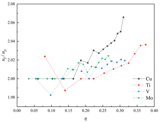
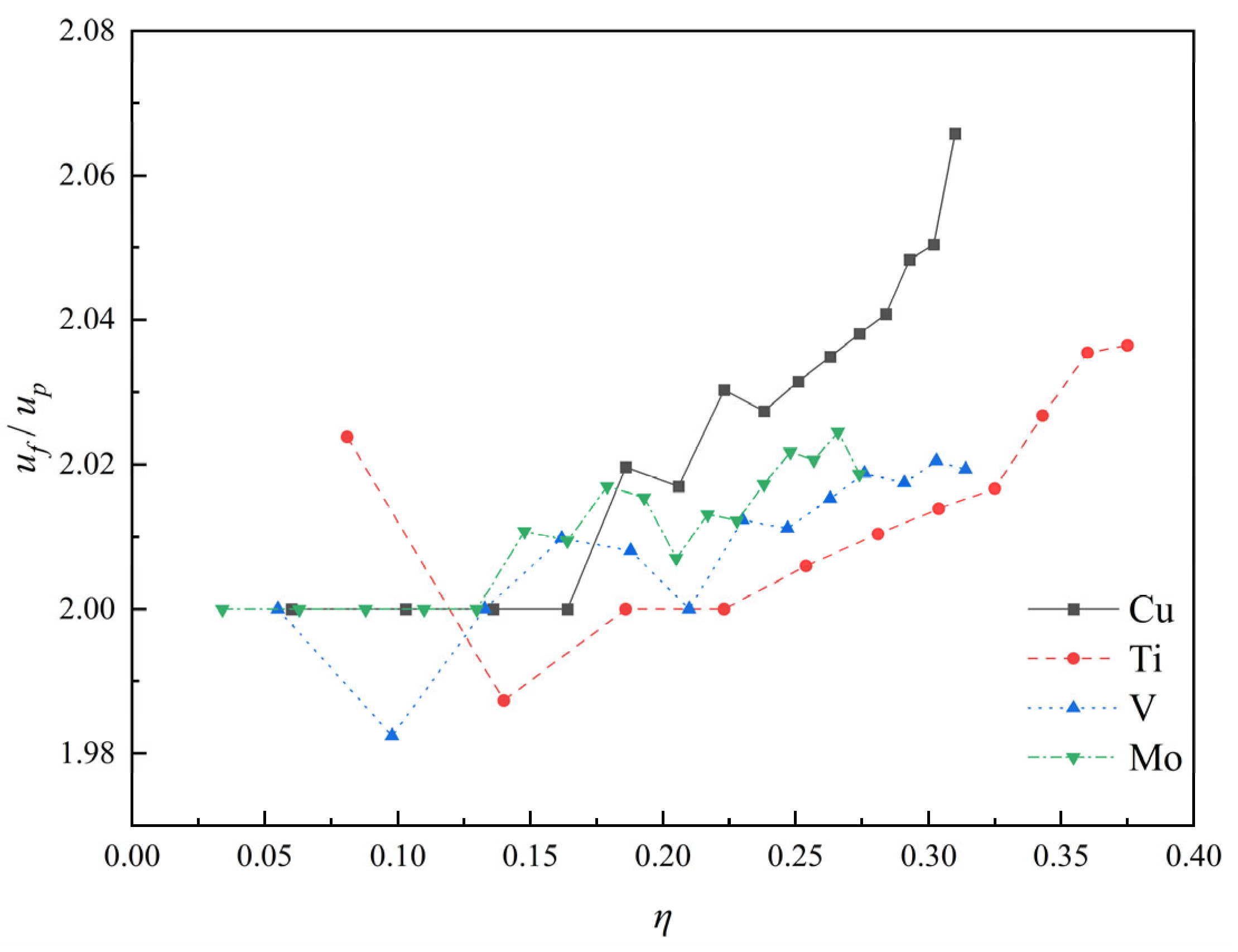
This result indicates that $u_f$ is about twice that of $\Delta u$, which is consistent with previous research and our experimental results [37,38,39]. As shown in Figure 13, for the strong impact relationship, as $\eta$ increases, $u_f/u_p$ shows a slight increase, but the maximum value does not exceed 2.07. Under weak impact conditions $\left(\eta \le 0.2\right)$, the maximum value of $u_f/u_p$ is about 2.02, with an error of only 1% compared to the estimated result. Under strong impact conditions $\left(\eta >0.2\right)$, the maximum value of $u_f/u_p$ is about 2.07. This indicates that the approximate method used in this article has high credibility and accuracy.

Figure 13. $u_f/u_p-\eta$ curves of four typical elements. Adapted from Ref. [36].

In the present model, the unloading stage is treated as a reverse Hugoniot, with the ratio of the unloading velocity to the particle velocity taken as $u_f/u_p=2$. This simplification implicitly assumes that the unloading path coincides with the mirror image of the principal Hugoniot, and thermal softening does not significantly alter the unloading modulus. In fact, the actual unloading isentrope often deviates from the reverse Hugoniot due to differences in entropy production between the loading and unloading paths. Furthermore, the intense adiabatic heating during shock compression can reduce the effective unloading stiffness, making the actual path softer than the reverse Hugoniot. These phenomena can lead to lower predictions of jet velocity by theoretical models. A preliminary sensitivity analysis suggests that the combined effect of these factors may introduce an uncertainty of approximately ±5% to ±10% in the predicted jet velocity.

4.4. Jet Velocity Synthesis

$V_J$ is divided into two vector sums, namely the collision point velocity $V_1$ (global reference frame) and the unloading acceleration $V_{\mathit{U}}$:

$$V_J=V_1+V_{\mathit{U}}$$

(34)

In the unloading stage, $V_{\mathit{U}}$ mainly consists of outflow velocity $V_3$ (collision-point reference frame) and unloading velocity $\Delta u$ (collision-point reference frame):

$$V_{\mathit{U}}=V_3+\Delta u$$

(35)

When the liner element is transformed into a jet element, all the pressure at the collision point is converted into the jet element’s kinetic energy. According to the Bernoulli equation, $V_3$ can be expressed as follows:

$$V_3=\sqrt{2p_H/{\rho }_1}$$

(36)

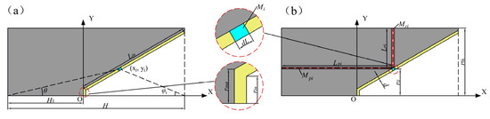
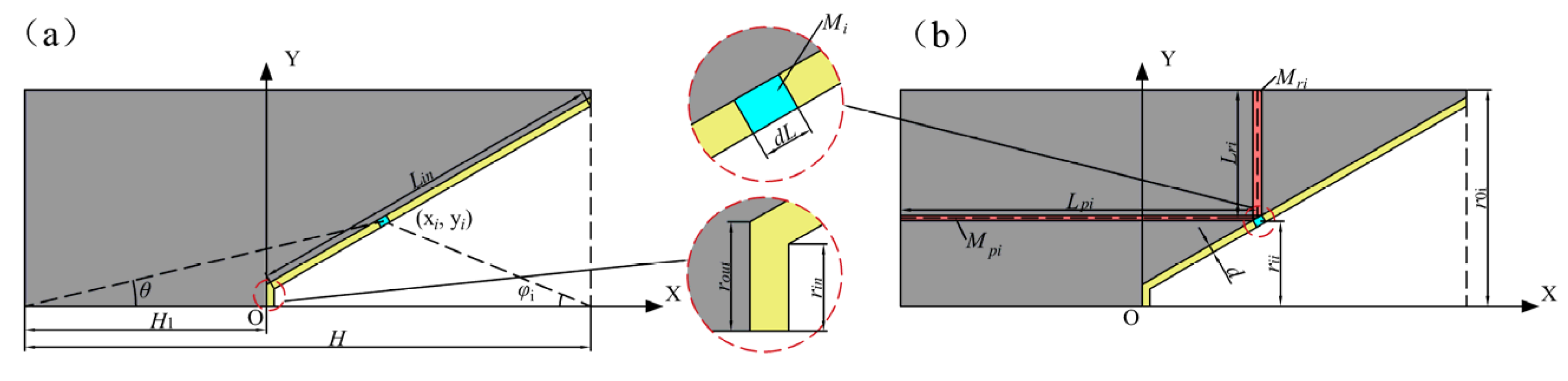
Figure 14 shows the calculation model for the collapse velocity of the liner element in the SC structure. As shown in Figure 14a, by establishing a coordinate system at the top of the liner and dividing it into N elements, the length of a single element $dL$ can be expressed as follows:

$$dL=L_{in}/N={\displaystyle \frac{H-H_1-d}{N\cos ({\alpha }_1)}}$$

(37)

where H is the height of the SC; H₁ is the distance from the top of the liner to the detonation center; d is the liner thickness; $L_{in}$ is the length of the busbar inside the liner; and ${\alpha }_1$ is the half-cone angle of the liner.

Figure 14. Schematic diagram of the collapse velocity calculation model. (a) structural parameters of SC (b) classification method for liner elements and corresponding explosives.

The coordinates of the element $\left(x_i,y_i\right)$ can be represented as follows:

$$\left\{\begin{array}{l}{x}_i=idL\cos ({\alpha }_1)+d-d\sin ({\alpha }_1)\\ y_i=idL\sin ({\alpha }_1)+r_{in}+d\cos ({\alpha }_1)\end{array}\right.$$

(38)

The collapse velocity of the liner element $V_{0i}$ can be expressed as follows due to the influence of axial and radial explosives during collapse [21]:

$$\left\{\begin{array}{l}{V}_{0i}=f\left({\phi }_i\right)V_{pi}+g\left({\phi }_i\right)V_{\mathit{r}i}\\ f\left({\phi }_i\right)=1-\sin {\phi }_i\\ g\left({\phi }_i\right)=\sin {\phi }_i\end{array}\right.$$

(39)

where ${\phi }_i$ is the angle between the line connecting the position of the liner element and the projection point of the liner mouth on the axis of symmetry to the axis of symmetry; and $V_{pi}$ and $V_{\mathit{r}i}$ are the axial velocity component and the radial velocity component of the element, respectively:

$$\left\{\begin{array}{l}{V}_{pi}=\sqrt{2E}{\left({\displaystyle \frac{{(1+2{\mu }_{pi})}^3+1}{6(1+{\mu }_{pi})}}+{\mu }_{pi}\right)}^{-1/2}\\ V_{ri}=\sqrt{2E}{\left({\displaystyle \frac{r_{0i}^2-r_{ii}^2}{r_{xi}^2-r_{ii}^2}}{\mu }_{ri}+{\displaystyle \frac{1}{6}}\right)}^{-1/2}\end{array}\right.$$

(40)

where $\sqrt{2E}$ is the characteristic velocity of the explosive, which is related to the type of explosive; ${\mu }_{pi}$ is the mass ratio of the liner element to the explosive in the axial direction; and ${\mu }_{ri}$ is the mass ratio of the liner element to the explosive in the radial direction.

Chantere [40] assumes that the pressure of the detonation gas is uniform and that there is an immovable cylindrical surface in the explosive. The surface radius of a stationary cylinder $r_x$ can be obtained by the following equation:

$$r_{xi}^3+3r_{xi}\left(\left(r_{0i}+r_{ii}\right){\displaystyle \frac{{\rho }_e}{{\rho }_{\mathit{CJ}}}}({\mu }_{ri}{r}_{0i}+{\mu }_{ki}{r}_{ii})+r_{ii}{r}_{0i}\right)-3\left(r_{0i}+r_{ii}\right)r_{ii}{r}_{0i}\left({\displaystyle \frac{2}{3}}+{\displaystyle \frac{{\rho }_e}{{\rho }_{\mathit{CJ}}}}({\mu }_{ri}+{\mu }_{ki})\right)=0$$

(41)

where $r_{0i}$ and $r_{ii}$ are the outer diameter and the inner diameter of the explosive corresponding to the element; ${\mu }_{ki}$ is the mass ratio of the shell corresponding to the element to the explosive; and ${\rho }_e$ and ${\rho }_{\mathit{CJ}}$ are the initial density and the C–J density of the explosive, respectively.

According to the method of dividing elements shown in Figure 14b, ${\mu }_{pi}$ and ${\mu }_{ri}$ can be represented as

$$\left\{\begin{array}{l}{\mu }_{pi}={\displaystyle \frac{M_i}{M_{pi}}}={\displaystyle \frac{{\rho }_{0}dL}{L_{pi}{\rho }_e}}\\ {\mu }_{ri}={\displaystyle \frac{M_i}{M_{ri}}}={\displaystyle \frac{{\rho }_{0}dL}{L_{ri}{\rho }_e}}\end{array}\right.$$

(42)

where $M_{pi}$ and $L_{pi}$ represent the mass and thickness of the explosive corresponding to the elements in the axial direction, respectively; and $M_{ri}$ and $L_{ri}$ are the mass and thickness of the explosive corresponding to the elements in the radial direction, respectively.

The projection angle ${\delta }_i$ of the liner element can be calculated as follows:

$${\delta }_i=\arcsin \left({\displaystyle \frac{V_{0i}\cos {\theta }_i}{2D_e}}\right)$$

(43)

where $D_e$ represents the detonation velocity of the explosive and ${\theta }_i$ is the angle between the detonation velocity vector and the tangent of the liner elements.

By combining Equation (37) with Equation (43), $V_{0i}$ can be calculated. When $V_{0i}$ is known, the flow velocity $V_{2i}$ and the collision point velocity of the element $V_{1i}$ can be solved based on geometric relationships:

$$\left\{\begin{array}{l}{V}_{1i}={\displaystyle \frac{V_{0i}}{\sin {\beta }_i}}cos\left({\beta }_i-{\alpha }_1-{\delta }_i\right)\\ V_{2i}={\displaystyle \frac{V_{0i}}{\sin {\beta }_i}}cos\left({\alpha }_1+{\delta }_i\right)\end{array}\right.$$

(44)

The collapse angle of the element ${\beta }_i$ can be expressed as follows:

$$\tan {\beta }_i={\left.{\displaystyle \frac{\partial r}{\partial x}}{\displaystyle \frac{\partial x}{\partial z}}\right|}_{r=0}={\displaystyle \frac{\sin \left({\alpha }_1+2{\delta }_i\right)-x_i\sin {\alpha }_1\left[1-\tan \left({\alpha }_1+{\delta }_i\right)\tan {\delta }_i\right]V_{0i}^{\prime }/V_{0i}}{\cos \left({\alpha }_1+2{\delta }_i\right)+x_i\sin {\alpha }_1\left[\tan \left({\alpha }_1+{\delta }_i\right)+\tan {\delta }_i\right]V_{0i}^{\prime }/V_{0i}}}$$

(45)

4.5. Dynamic Yield Strength Solution Method Based on J-C Model

During impact compression, the material’s dynamic yield strength can affect the efficiency of momentum conversion. This Section aims to establish a solution method based on the J–C constitutive model to obtain a dynamic yield strength $\sigma$ that represents the entire impact compression process. In the collision zone, the material experiences high strain rates and plastic deformation, and the temperature rises significantly. Assuming the material reaches a relatively stable state after the shock wave front, the J–C model is used to estimate its dynamic yield strength.

Assuming that the plastic work of the material is used for temperature rise [41,42]:

$$\Delta \mathrm{T}={\displaystyle \frac{0.9{\displaystyle {\int }_0^{{\epsilon }_p}\sigma d\epsilon }}{\rho Cv}}$$

(46)

Substituting Equation (3) into Equation (46) yields the following Equation (47):

$$F\left({\epsilon }_p\right)=0.9\left(A+B{\epsilon }_p^n\right)\left(1+C\ln {\dot{\epsilon }}_p\right)\left(1-T^{*m}\right){\epsilon }_p-\Delta T=0$$

(47)

Equation (47) is an implicit equation about ${\epsilon }_p$, which can be solved using Newton’s iterative method:

$${\epsilon }_p^{\left(k+1\right)}={\epsilon }_p^{\left(k\right)}-{\displaystyle \frac{F\left({\epsilon }_p^{\left(k\right)}\right)}{F^{\prime }\left({\epsilon }_p^{\left(k\right)}\right)}}$$

(48)

where $F^{\prime }\left({\epsilon }_p\right)=dF/d{\epsilon }_p$.

To solve $\sigma$, it is also necessary to know the material’s dynamic strain rate ${\dot{\epsilon }}_{dyn}$ in the collision zone. During the impact compression process, the material undergoes rapid loading, with $\dot{\epsilon }$ reaching 10⁵–10⁷ s⁻¹ [25]. Therefore, in the calculation of this article, ${\dot{\epsilon }}_{dyn}={10}^6$ is used.

5. Discussion and Analysis

TC21 and Ti₅₅Al₂₀V₅Zr₅Nb₁₅ HEA have similar material properties. In contrast, the Ti₅₅Al₂₀V₅Zr₅Nb₁₅ HEA achieves a slightly lower jet velocity (6982 m/s) but maintains better cohesiveness, suggesting a more favorable balance between energy storage and release during unloading. Therefore, a comparative analysis of Cu and Ti₅₅Al₂₀V₅Zr₅Nb₁₅ HEA will be conducted in this Section.

5.1. Calibration of Dynamic Momentum Conversion Factor

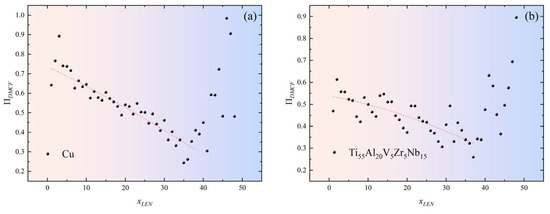
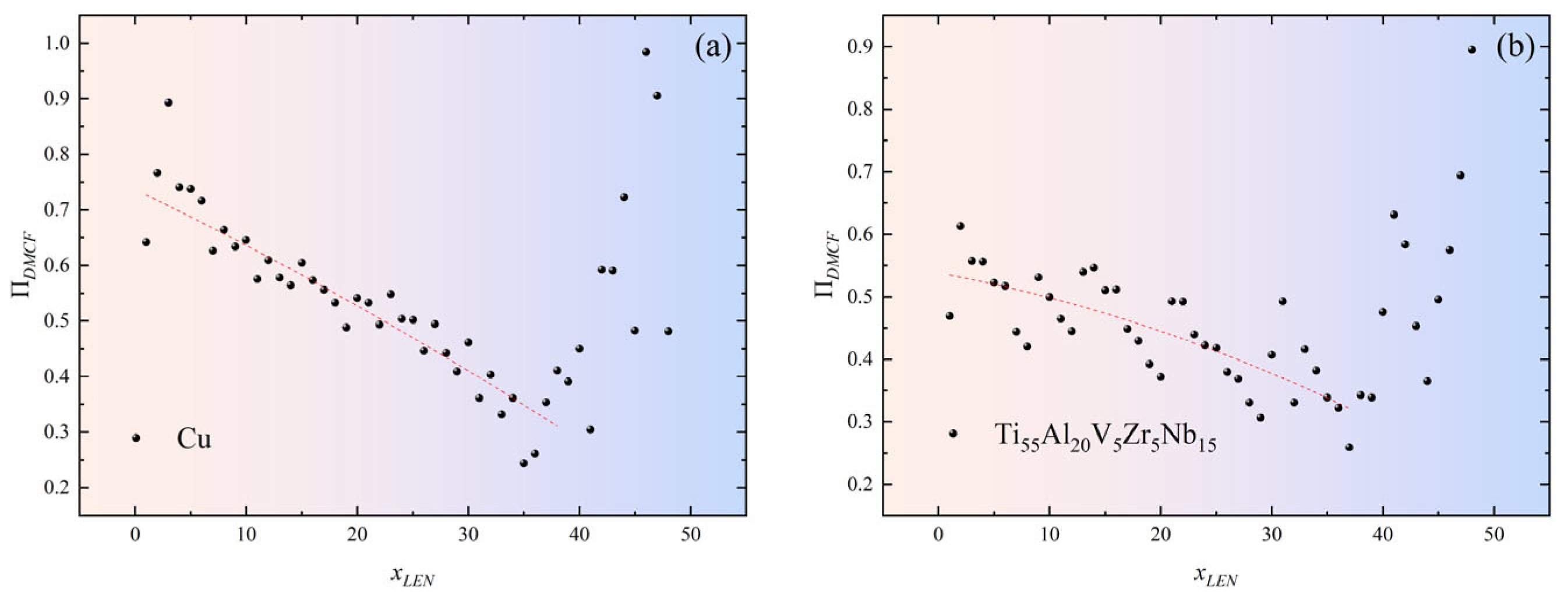
By extracting the $V_{n2}$ and $V_r$ values of all the elements in the high-fidelity numerical simulations, as shown in Figure 15, a decreasing trend in ${\Pi }_{DMCF}$ is observed as the element coordinates $x_{LEN}$ increase. However, after Gauge # 40, ${\Pi }_{DMCF}$ shows an abnormal increase. This phenomenon arises from the spatial distribution characteristics of Gauge points in numerical simulations: the positions of Gauges # 40~48 are close to the outside of the liner, and during their movement, some areas flow into the air domain, resulting in a data acquisition distortion of $V_r$. However, Gauges # 44~48, due to their low collapse velocity, are unable to fully participate in jet formation, further reducing the accuracy of the data collection.

Figure 15. Numerical calculation results: (a) Cu; (b) Ti₅₅Al₂₀V₅Zr₅Nb₁₅ HEA.

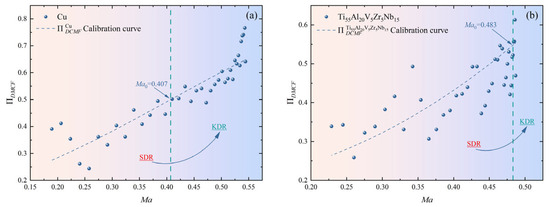
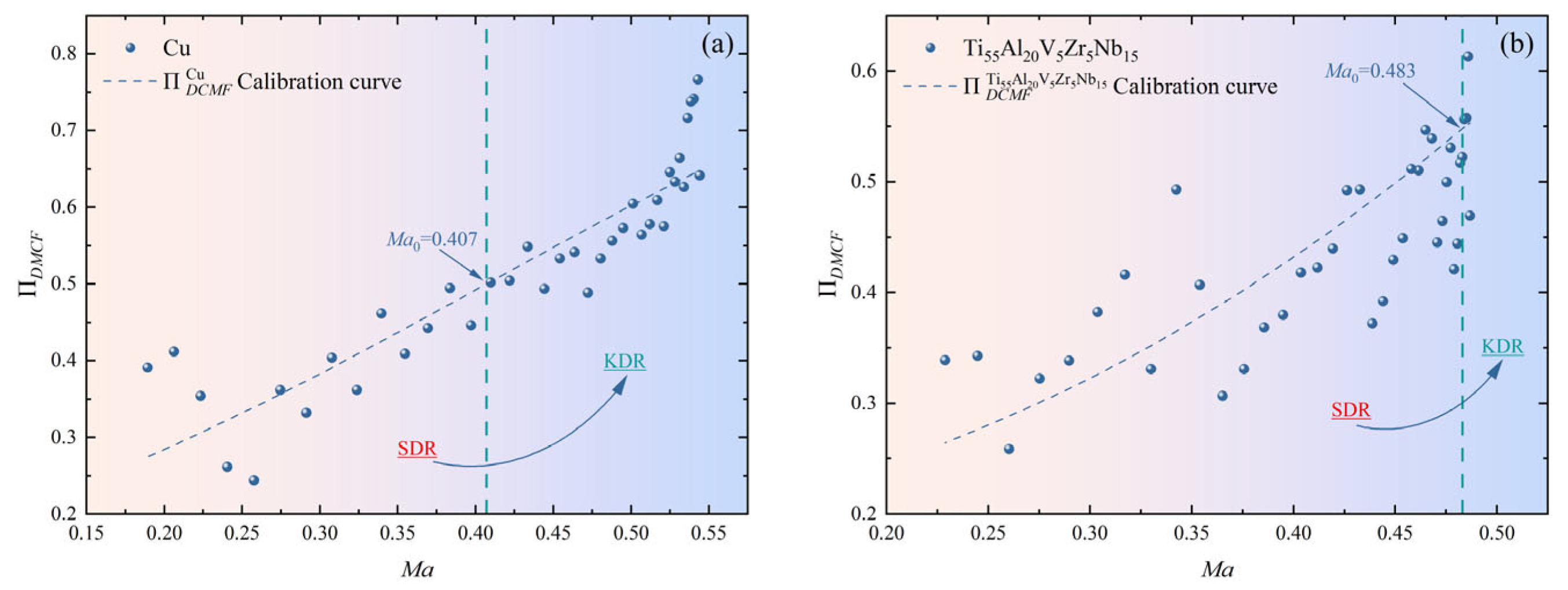
As shown in Figure 16, ${\Pi }_{DMCF}$ shows a monotonically increasing trend with $Ma$. For the same $Ma$, Cu has a higher ${\Pi }_{DMCF}$. In addition, the position of $M{a}_0$ is marked in the Figure 16. On the left side of $M{a}_0$ is the strength-dominated regime (SDR), where $Ma\le M{a}_0$. On the right side of $M{a}_0$ is the kinetic-dominated regime (KDR), where $Ma\gg M{a}_0$. By comparison, most of the elements in the Ti₅₅Al₂₀V₅Zr₅Nb₁₅ HEA are located in the SDR. This means that the majority of the normal momenta of the elements during collision is not converted into impact momentum, resulting in decreased shock pressure and compressibility of the material. In addition, the SDR range of the Ti₅₅Al₂₀V₅Zr₅Nb₁₅ HEA is larger. Therefore, the Ti₅₅Al₂₀V₅Zr₅Nb₁₅ HEA may be more difficult to overcome the transition from the SDR to the KDR. Since most Cu elements are located in the KDR, their dynamic response in the collision region is closer to that of an ideal fluid, resulting in higher shock pressure and compressibility.

Figure 16. Calibration curves of ${\Pi }_{DMCF}$ for (a) Cu and (b) Ti₅₅Al₂₀V₅Zr₅Nb₁₅ HEA.

The parameters Ma₀ and k are calibrated using a dataset generated from the numerical simulations covering the Ti₅₅Al₂₀V₅Zr₅Nb₁₅ HEA and Cu jets. The calibration procedure consists of the following steps. Firstly, based on the theoretical model, $V_{2i}$ and ${\beta }_i$ are obtained, and Ma is calculated. Secondly, $V_{\mathit{n}2}$ and $V_r$ are extracted from the numerical simulation, and ${\Pi }_{DMCF}$ is calculated. It is necessary to associate the Ma of the different elements with their corresponding momentum conversion efficiencies and establish a distribution curve of momentum conversion efficiency. Finally, the logistic function is used to fit the curve and obtain the corresponding fitting parameters $M{a}_0$ and $k$.

Table 8 presents the parameter calibration results for the logistic function. Due to the large fluctuation range in the numerical calculation results for the Ti₅₅Al₂₀V₅Zr₅Nb₁₅ HEA, the fit for Cu is higher (R² = 0.816) than for the Ti₅₅Al₂₀V₅Zr₅Nb₁₅ HEA (R² = 0.589). The $k$ value for Cu is higher, indicating that the transition rate of Cu from the SDR to the KDR is faster.

Table 8. Calibration parameters of ${\Pi }_{DMCF}$.

Material	$\mathit{M}{\mathit{a}}_0$	$\mathit{k}$	${\mathit{R}}^2$
Cu	0.407	4.46	0.816
Ti55Al20V5Zr5Nb15	0.483	3.48	0.589

5.2. Theoretical and Numerical Comparative Analysis of Dynamic Yield Strength

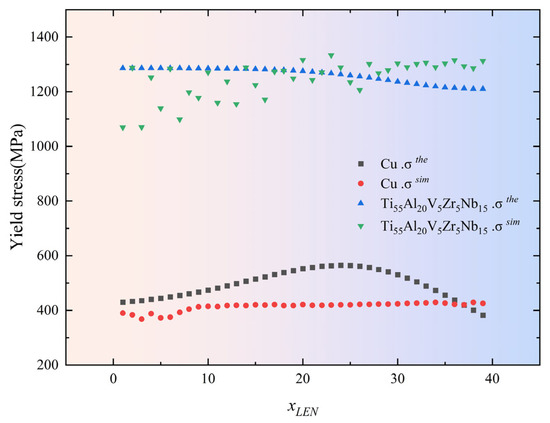
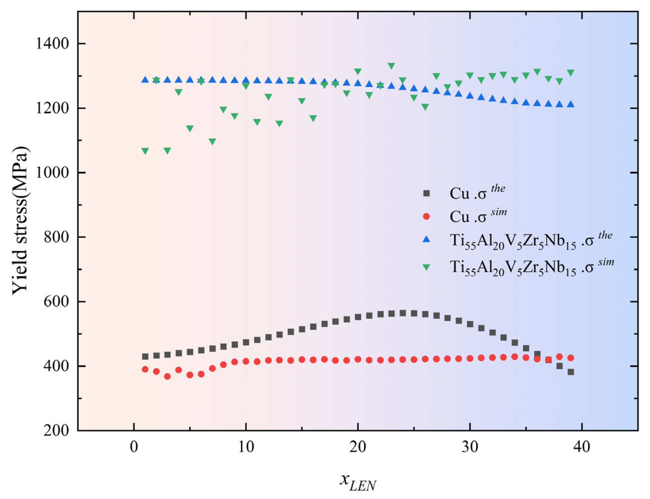
To verify the reliability of the theoretical model, the numerical results ${\sigma }^{sim}$ are compared with the theoretical calculations ${\sigma }^{the}$. As shown in Figure 17, as $x_{LEN}$ increases, ${\sigma }^{sim}$ gradually increases. Overall, the yield strength of the Ti₅₅Al₂₀V₅Zr₅Nb₁₅ HEA is significantly higher than that of Cu. Combined with Figure 16, this higher yield strength results in poorer plastic flow and a smaller ${\Pi }_{DMCF}$ in the collision zone. When the change in yield strength is not significant, the material with a lower impact strength has a smaller ${\Pi }_{DMCF}$. A smaller ${\Pi }_{DMCF}$ leads to a lower effective pressure ratio for driving the unloading acceleration, resulting in a lower jet velocity.

Figure 17. ${\sigma }^{sim}$ vs. ${\sigma }^{the}$.

Compared to Cu, the ${\sigma }^{sim}$ of the Ti₅₅Al₂₀V₅Zr₅Nb₁₅ HEA increases slowly, but the overall fluctuation amplitude is large. Based on the theoretical model, the ${\sigma }^{the}$ and the ${\sigma }^{sim}$ differ significantly. For Cu, the ${\sigma }^{the}$ and the ${\sigma }^{sim}$ of the top and bottom elements match well, whereas in the middle element, the ${\sigma }^{the}$ is significantly higher than the ${\sigma }^{sim}$. This discrepancy may be due to the theoretically calculated impact temperature $T_1^{the}$ being lower than the numerically calculated impact temperature $T_1^{sim}$, resulting in the ${\sigma }^{the}$ being too high. Due to the greater thermal softening effect of the Ti₅₅Al₂₀V₅Zr₅Nb₁₅ HEA than that of Cu, temperature is no longer the main factor. The main reason may be that less plastic work is required for heating, resulting in ${\sigma }^{the}$ being less than ${\sigma }^{sim}$.

For this irregular fluctuation, the average value ${\sigma }_{avg}$ is used for comparison, and the comparison results are shown in Table 9. The dynamic yield strength of the Cu material (494 MPa) is about 4.6 times the initial yield strength (90 MPa), while the dynamic yield strength (1261 MPa) of the Ti₅₅Al₂₀V₅Zr₅Nb₁₅ HEA is about 1.3 times the initial yield strength (965 MPa). This indicates that during the collapse stage, the thermal softening effect of the Ti₅₅Al₂₀V₅Zr₅Nb₁₅ HEA dominates, whereas the thermal softening effect of Cu is relatively weak. The theoretical model’s maximum error is +19.6% (Cu), and the minimum error is only +1.12% (Ti₅₅Al₂₀V₅Zr₅Nb₁₅ HEA). The error between the theoretical model and the previous experimental results (571.6 MPa) is −13.5% [25]. The theoretical model’s error is kept within 20%, indicating that the model can predict the dynamic yield strength of the materials well. According to Table 8, materials with a high yield strength have a larger $M{a}_0$ and a smaller $k$. This indicates that the dynamic yield strength of the material will affect the values of $M{a}_0$ and $k$. $\sigma$ is positively correlated with $M{a}_0$ and negatively correlated with $k$. Materials with a higher dynamic yield strength reduce compressibility, so most of the material’s normal momentum is used for plastic deformation, decreasing shock pressure and ${\Pi }_{DMCF}$.

Table 9. ${\sigma }_{avg}^{sim}$ vs. ${\sigma }_{avg}^{the}$.

Material	A/MPa	Average		Error/%
		${\mathit{\sigma }}_{\mathit{avg}}^{\mathit{the}}$/MPa	${\mathit{\sigma }}_{\mathit{avg}}^{\mathit{sim}}$/MPa
Cu	90	494	413	+19.6
Ti55Al20V5Zr5Nb15	965	1261	1247	+1.12

5.3. Theoretical Model Validation and Evaluation

To verify the reliability and accuracy of the theoretical model, the coefficient of determination (R²) is used to assess the degree of agreement between the theoretical and computational results for $p_H$:

$$R^2=1-{\displaystyle \frac{S{S}_{res}}{S{S}_{tot}}}=1-{\displaystyle \frac{{\displaystyle \sum _{i=1}^N{\left(p_i-{\widehat{p}}_i\right)}^2}}{{\displaystyle \sum _{i=1}^N{\left(p_i-{\overline{p}}_i\right)}^2}}}$$

(49)

where $S{S}_{res}$ is the sum of squared residuals; $S{S}_{tot}$ is the total sum of squares; $p_i$ is the numerical calculation result; ${\widehat{p}}_i$ is the theoretical calculation result; and ${\overline{p}}_i$ is the mean of the numerical calculation results.

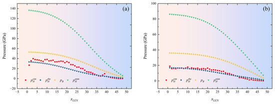
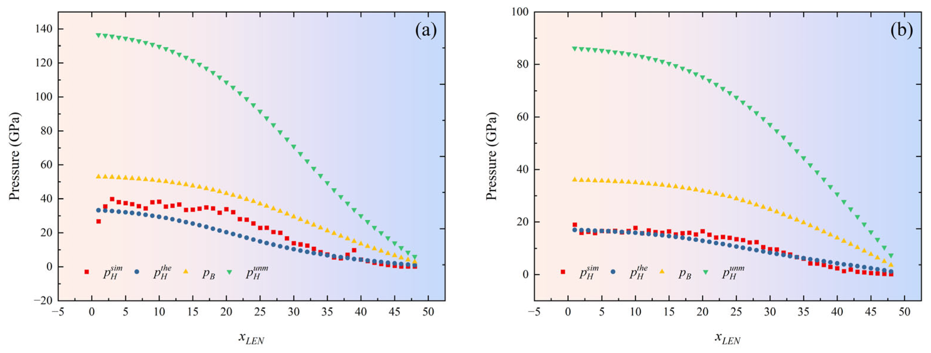
The values of $p_H$ and $V_J$ for the two materials are calculated based on the calibration curve of ${\Pi }_{DMCF}$. The differences among the theoretical $p_H^{the}$, the numerical $p_H^{sim}$, the Bernoulli $p_B$, and the uncorrected Hugoniot pressure $p_H^{unm}$ results are compared and analyzed, as shown in Figure 18.

Figure 18. Comparison of theoretical and numerical calculation results of $p_H$ for (a) Cu and (b) Ti₅₅Al₂₀V₅Zr₅Nb₁₅ HEA.

As $x_{LEN}$ increases, $p_H$ shows a gradually decreasing trend. A comparative analysis reveals that, owing to the lower dynamic yield strength, the Cu liner’s flowability during collision is better, with a higher ${\Pi }_{DMCF}$ and $p_H$. Materials with a higher $p_H$ mean that the liner is more fully compressed during collapse, resulting in better jet cohesion in the subsequent formation. The experimental and numerical results also support this point. In addition, compared to $p_H^{the}$, $p_B$ and $p_H^{unm}$ are significantly higher than $p_H^{sim}$. This indicates that the effective pressure used to drive the unloading acceleration is significantly lower.

Table 10 compares the errors of three methods for determining $p_H$. Compared with the others, the model proposed in this article achieves a high-precision prediction of $p_H$, with R² values of 0.778 and 0.943. The prediction accuracy for $p_B$ and $p_H^{unm}$ is significantly lower than that for $p_H^{the}$, indicating that the theoretical model proposed in this paper accurately predicts the $p_H$ of the jet, providing theoretical support for the design of SC structures.

Table 10. Comparison of errors between theoretical and numerical calculation results.

Pressure	R2
	Cu	Ti55Al20V5Zr5Nb15
$p_H^{the}$	0.778	0.943
$p_B$	0.154	−5.183
$p_H^{unm}$	−23.654	−71.320

5.4. Material Applicability Analysis

The theoretical model proposed in this article requires numerical calculations to calibrate ${\Pi }_{DMCF}$ to improve the accuracy of the model predictions. To verify the applicability of the material and the model results, jet velocities are predicted for seven additional commonly used materials using the theoretical models. We compare the theoretical calculation results $V_J^{the}$, the PER model calculation results $V_J^{PER}$, and the experimental results $V_J^{exp}$, as shown in Table 11. Due to significant variation in the dynamic yield strength with structural changes, the material’s initial yield strength is provided as a reference in the Table.

Table 11. Comparison of jet velocities for typical materials.

Material	A/MPa	C0/(m/s)	Velocity/(m/s)			Error/%		Reference
			${\mathit{V}}_{\mathit{J}}^{\mathit{the}}$	${\mathit{V}}_{\mathit{J}}^{\mathit{PER}}$	${\mathit{V}}_{\mathit{J}}^{\mathit{exp}}$	${\mathit{V}}_{\mathit{J}}^{\mathit{the}}$	${\mathit{V}}_{\mathit{J}}^{\mathit{PER}}$
Cu	90	3940	6827	7155	6916	1.28	3.5	[17]
					6498	5.06	10.1	[25]
					6251	9.21	14.5	[27]
CMS	430	3814	6913	7159	6447	7.50	11.0
CMZ	206	3834	6851	7204	6363	7.67	13.2
Steel1006	350	4569	6648	7274.3	6702	0.81	8.5	[31]
HNS	500	4569	6625	7267.3	6636	1.66	9.5
Mo	300	5124	6228	7026	6421	3.00	9.4	[25]
TC21	1030	5110	7296	7691	7236	0.83	6.3	[31]
TB6	797	5031	7289	7672	7271	0.24	5.5
Ti55Al20V5Zr5Nb15	965	5026	7204	7665	6982.1	3.18	9.8	[8]

The theoretical model has a minimum error of only 0.24% (TB6) and a maximum of 9.21% (Cu). By comparison, the PER theory has a minimum error of 3.5% (Cu) and a maximum of 13.2% (CMZ). This indicates that the model proposed in this article performs particularly well for high-sound-velocity materials such as Steel1006, HNS, TC2, TB6, and Ti₅₅Al₂₀V₅Zr₅Nb₁₅ HEA, with errors kept within 4%. For low-sound-velocity materials (Cu, CMS, CMZ), the error remains within 10%. It is worth noting that for medium-sound-velocity materials (Steel1006 and HNS), since their ${\Pi }_{DMCF}$ have not been calibrated through numerical calculations, ${\Pi }_{DMCF}^{{\mathrm{Ti}}_{55}\mathrm{A}{\mathrm{l}}_{20}{\mathrm{V}}_5\mathrm{Z}{\mathrm{r}}_5\mathrm{N}{\mathrm{b}}_{15}}$ is used in the calculation. In the end, the predicted results are slightly smaller than the experimental results. The reason for this phenomenon is that their yield strength and sound velocity are both lower than for the Ti₅₅Al₂₀V₅Zr₅Nb₁₅ HEA, resulting in differences in their actual calibration parameters.

Based on the calibration parameters of Cu and Ti₅₅Al₂₀V₅Zr₅Nb₁₅ HEA, the calibration parameters for Steel1006 and HNS are obtained using linear interpolation. The linear interpolation formula is

$$y_3=y_1+\left(y_2-y_1\right)\times \left(x_3-x_1\right)/\left(x_2-x_1\right)$$

(50)

where $\left(x_1,y_1\right)$ and $\left(x_2,y_2\right)$ are known data points and $\left(x_3,y_3\right)$ is an unknown data point.

As shown in Table 12, the theoretical model’s predictions are generally higher than the experimental results, and the errors are kept within 1.5%. This indicates that the calibration parameters obtained via linear interpolation can be used to predict jet velocity with the theoretical model. In addition, for materials with similar sound velocity and yield strength, their jet velocity and error are not significantly different.

Table 12. Calibration parameters and prediction results.

Material	$\mathit{M}{\mathit{a}}_0$	$\mathit{k}$	${\mathit{V}}_{\mathit{J}}^{\mathit{the}}/\left(\mathbf{m}/\mathbf{s}\right)$	${\mathit{V}}_{\mathit{J}}^{\mathit{exp}}/\left(\mathbf{m}/\mathbf{s}\right)$	Error/%
Steel1006	0.451	3.89	6757	6702	0.82
HNS			6733	6636	1.46

This phenomenon indicates that, under the same SC structure, materials with a similar sound velocity and yield strength (i.e., TC21, TB6, and Ti₅₅Al₂₀V₅Zr₅Nb₁₅ HEA; CMZ and CMS; and Steel1006 and HNS) can use the same ${\Pi }_{DMCF}$ to predict the jet velocity. For materials with a similar sound velocity and a higher yield strength (Cu, CMS, and CMZ), using the same ${\Pi }_{DMCF}$ to predict the jet velocity may result in higher prediction results. This phenomenon further indicates that the high yield strength of the material leads to an increase in $M{a}_0$ and a decrease in $k$. At the same $Ma$, the ${\Pi }_{DMCF}$ of low-strength materials is larger.

In summary, the theoretical model proposed in this article can achieve a high-precision prediction of jet velocity. Compared with the traditional PER theoretical models, this model’s error does not exceed 10%. For high-sound-velocity, high-strength materials, the error is even lower, at no more than 4%, demonstrating ultra-high reliability and broad material applicability. In addition, when the calibration parameters for the dynamic momentum conversion factors are known for materials with different sound velocity, those for unknown materials can be obtained via linear interpolation, greatly reducing the time and computational costs of numerical calculations.

Overall, the work of this article focused on two stages: shock compression and unloading acceleration. Compared with traditional theoretical frameworks [13,18,23], the model proposed in this article has a wider range of material applications and higher accuracy. In addition, the potential relationships between material strength, shock pressure and jet velocity were also revealed. In terms of industrial significance, we further point out that this model provides theoretical guidance for the composition design and geometric optimization of an HEA liner. For example, by adjusting the Grüneisen coefficient of the HEA, the compression unloading path can be optimized, thereby improving cohesiveness while maintaining jet velocity. This understanding is expected to drive the development of a new generation of high-performance SC warheads.

5.5. Parameter Sensitivity Analysis

Although the analytical model established in Chapter 4 offers high computational efficiency, its simplified assumptions may introduce systematic errors in complex compression and unloading processes. Therefore, this Section will systematically evaluate the extent to which uncertainty in the key input parameters of the model established in this article affects the final output. By quantifying the sensitivity of each parameter, the model’s robustness can be assessed, and the core factors that dominate the jet-forming process can be identified, providing clear optimization directions for liner material selection.

Using the single factor perturbation method for analysis, under the reference operating conditions, a certain input parameter is allowed to vary within its reasonable uncertainty range (±20%), while all the other parameters are fixed, and the amplitude of the output change is observed.

We define the normalized sensitivity coefficient $S_P^Q$ to quantify the impact of parameter P on output Q as follows:

$${\psi }_P^Q={\displaystyle \frac{\Delta Q/Q_{base}}{\Delta P/P_{base}}}$$

(51)

where $\Delta Q$ and $\Delta P$ are the changes in output and input, respectively, and the subscript “base” represents the reference value. $\left|\psi \right|>1$ represents high sensitivity; $0.5<\left|\psi \right|<1$ represents moderate sensitivity; and $\left|\psi \right|<0.5$ represents low sensitivity.

The analysis parameters mainly focus on the material’s own properties, as shown in Table 13. The range of the parameter change rate is ± 20%. Under the reference operating conditions, we let a certain input parameter vary within its reasonable uncertainty range while fixing all the other parameters, and we observe the magnitude of the change in the output variable.

Table 13. Parameters used for sensitivity analysis.

Number	Input	Reference
1	${\rho }_0$	8.93 g/cm3
2	${\Pi }_{DMCF}$	0.6
3	$C_0$	3940 m/s
4	$S$	1.489
5	$V_0$	2743 m/s

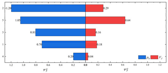
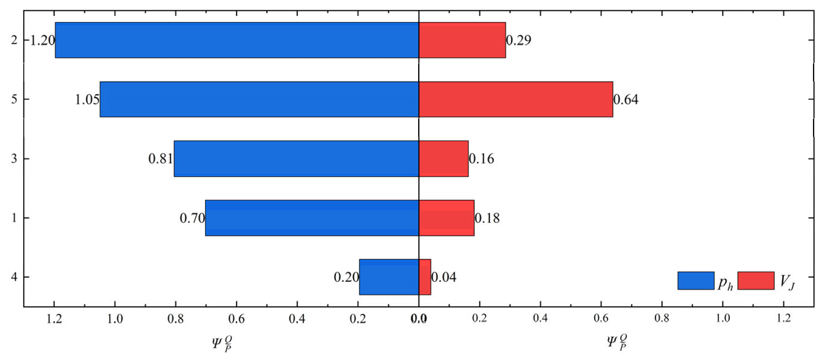
Based on the above method, the sensitivity of $V_J$ and $p_H$ to the key parameters is obtained, as shown in Figure 19. This graph illustrates how changes in each parameter within ±20% affect $V_J$ and $p_H$. The longer bars indicate higher sensitivity: the parameters ${\Pi }_{DMCF}$ and $V_0$ show high sensitivity, ${\rho }_0$ and $C_0$ moderate, and $S$ low. ${\Pi }_{DMCF}$ shows moderate sensitivity to $V_0$ and low sensitivity to the other parameters, but among them, the parameter ${\Pi }_{DMCF}$ has the highest contribution ranking to $V_J$ (0.29). This indicates that momentum conversion is the core component of jet acceleration.

Figure 19. Parameter sensitivity analysis Tornado plot (absolute value).

It is worth noting that the $C_0$ and $V_0$ values of the Ti₅₅Al₂₀V₅Zr₅Nb₁₅ HEA are also higher than those of Cu, with only the ${\Pi }_{DMCF}$ and ${\rho }_0$ values lower than those of Cu. However, both the numerical and the theoretical calculations have shown that the Cu material has a higher shock pressure and better cohesiveness. The reason for this phenomenon is that the dynamic yield strength and sound velocity of the Ti₅₅Al₂₀V₅Zr₅Nb₁₅ HEA are higher (Figure 17), making it difficult for them to undergo the $M{a}_0$ transition from the SDR to the KDR. These issues all result in a lower ${\Pi }_{DMCF}$ and significantly smaller $p_H$ values for the Ti₅₅Al₂₀V₅Zr₅Nb₁₅ HEA.

The parameter sensitivity analysis shows that the model’s behavior in this article is consistent with physical intuition, and that the key outputs are dominated by clear physical mechanisms. ${\Pi }_{DMCF}$ is a key bridge connecting the dynamic properties of the materials with macroscopic jet performance. The analysis results provide a clear priority list and a quantitative basis for selecting and designing medication mask materials, significantly enhancing the practical engineering value of this theoretical model.

6. Conclusions

This study focuses on the core physical chain of “shock unloading” in the formation of SCJs and establishes an explicit theoretical model for unloading acceleration driven by shock pressure. Through systematic theoretical analysis, numerical simulation, and experimental verification, the following main conclusions have been drawn:

• This article constructs a quantitative model of “shock-pressure-driven unloading acceleration” with clear physical images. This model breaks with the simplification of the unloading acceleration stage in traditional theory and, for the first time, derives an explicit functional relationship between the unloading acceleration and the shock pressure at the collision point. It clarifies that shock pressure is the direct physical source of the kinetic energy acquired by the jet during the unloading stage, thereby significantly enhancing the physical transparency of the theoretical model.
• This article defines and calibrates a dynamic momentum conversion factor ${\Pi }_{DMCF}$ with universal significance, revealing its S-shaped evolution law with $Ma$ evolution. The research has shown that ${\Pi }_{DMCF}$ is not an empirical constant, and its evolution as a function of $Ma$ can be described by the logistic function. The model parameters ($M{a}_0$ and $k$) have clear physical meanings, representing the transition rate and the critical conditions, respectively. For the first time, the transition of material behavior from “strength dominant” to “kinetic dominant” has been clearly depicted.
• This article reveals the physical connotations of the key parameters ($M{a}_0$ and $k$) in the model and establishes their correlation with material properties. The parameter calibration results indicate that $M{a}_0$ directly reflects the impact-strength threshold required for the material to achieve moderate momentum-conversion efficiency and is positively correlated with the yield strength. $k$ characterizes the degree of abrupt transformation and is negatively correlated with the yield strength.
• The theoretical model established in this article exhibits excellent prediction accuracy and robustness on various materials. Verified by X-ray experiments, the prediction error in the jet head velocity of the Ti₅₅Al₂₀V₅Zr₅Nb₁₅ HEA is less than 4%. The theoretically predicted shock pressure is highly consistent with the high-fidelity numerical simulation results and significantly more accurate than the traditional models $\left({\mathrm{R}}^2=0.943\right)$. In addition, for eight typical materials with high sound velocity and high strength, the model’s prediction accuracy does not exceed 8%.
• This study has clarified that the yield strength of a material is a key internal factor in regulating the efficiency of momentum conversion and determining the performance of jet terminals. The research has shown that high-strength materials have higher alpha values and are in an SDR under the same collision conditions, which explains why the shock pressure of high-strength, high-sound-velocity materials may be lower than that of low-strength, low-sound-velocity materials. This conclusion provides direct theoretical guidance for the optimization and matching design of liner materials for specific penetration requirements.

The experimental data in this study are based on a single HEA composition and a single liner geometry, with a limited number of repeat tests. Conditions such as varying standoff distances and target obliquity are not explored. Therefore, the generalizability of the current conclusions requires further validation across a broader parameter space. For high-strength, multiphase HEA materials, simplifying the unloading path may introduce deviations. In addition, the calibration of the logistic parameters relies on the numerical simulation results and has not yet achieved predictions based entirely on physical parameters. Building on the present work, the following avenues are recommended for future investigation: (i) systematic experimental screening of HEA compositions with varying strength, impedance, and Grüneisen parameters; (ii) development of a machine-learning-based surrogate model for logistic parameter prediction.

References

- Zhang, Z.; Jin, W.W. Finite element modeling of the shaped charge jet and design of the reusable perforating gun. Pet. Sci. 2020, 17, 1389–1399. [Google Scholar] [CrossRef] [Scilit]
- Xu, G.; Wang, J.; Shi, M.; Zeng, J.; Li, H.; Yao, Q.; Huang, G. Application of shaped charge hydraulic smooth blasting technology in excavation of arc-shaped tunnel. Tunn. Undergr. Space Technol. 2026, 168, 107118. [Google Scholar]
- Reboul, N.; Chinnayya, A.; Paintendre, F.; Piagge, S.D.; Jaulin, V.; Limido, J.; Collé, A.; Rondot, F. Experimental and numerical study of the interaction between a shaped charge jet and a single ERA moving plate. Def. Technol. 2025, 50, 126–140. [Google Scholar]
- Ma, S.; Li, X.; Zhou, L. Experimental and numerical investigation of cavity characteristics in behind-armor liquid-filled containers under shaped charge jet impact. Def. Technol. 2025, 47, 242–259. [Google Scholar]
- Zhang, Z.; Yang, S.; Zhang, S.; Wang, L.; Sui, Y.; Li, T.; Zhang, G. Experimental study of damage to double-hull structure by underwater explosions of three charge types-blasting, shaped, and linear shaped charges. Int. J. Impact Eng. 2025, 203, 105369. [Google Scholar]
- Niu, Y.; Jia, X.; Zu, X.; Huang, Z. Research on the resistance of rock-rubble concrete to shaped charge jet penetration: The role of aggregate characteristics. Constr. Build. Mater. 2026, 513, 145424. [Google Scholar] [CrossRef] [Scilit]
- Liu, X.; Lu, Y.; Wang, X.; Liu, K.; Wang, L.; Feng, X.; Wang, B.; Jin, K.; Sun, S.; Cao, T.; et al. Moderating jet coherency to enhance the aftereffect damage while retaining desired penetration capability of shaped charge liners with Ti-Zr-Nb-Al energetic high-entropy alloys. J. Alloys Compd. 2025, 1035, 181585. [Google Scholar]
- Wang, Y.; Zu, X.; Huang, Z.; Xiao, Q.; Jia, X. The application of refractory high entropy alloys in shaped charge. Lat. Am. J. Solids Struct. 2025, 22, e8579. [Google Scholar] [CrossRef] [Scilit]
- Fang, Y.; Zhang, X.; Xiong, W.; Feng, K.; Liu, C.; Ge, X. Study on penetration law of shaped charge jet considering shape distribution characteristics. Trans. Beijing Inst. Technol. 2023, 43, 1047–1058. [Google Scholar]
- Gu, Y.; Wang, J.; Li, H.; Tang, K.; Liu, L. Formation characteristics and penetration performance of an underwater shaped charge jet. Ocean. Eng. 2022, 258, 111695. [Google Scholar] [CrossRef] [Scilit]
- Żochowski, P.; Warchoł, R. Experimental and numerical study on the influence of shaped charge liner cavity filing on jet penetration characteristics in steel targets. Def. Technol. 2023, 23, 60–74. [Google Scholar] [CrossRef] [Scilit]
- Walters, W.; Ground, A.P. An overview of the shaped charge concept. In Proceedings of the 11th Annual ARL/USMA Technical Symposium, West Point, NY, USA, 5–7 November 2003; ARL/USMA: West Point, NY, USA, 2003; Volume 5. [Google Scholar]
- Birkhoff, G.; MacDougall, D.P.; Pugh, E.M.; Taylor, S.G. Explosives with lined cavities. J. Appl. Phys. 1948, 19, 563–582. [Google Scholar] [CrossRef] [Scilit]
- Yin, X.; Yang, M.; Lai, J.; Du, L.; Zhou, J. Mechanism and maximum interference model of functionally graded concrete with liquid composite aggregates subjected to shaped charge jet penetration. Constr. Build. Mater. 2025, 476, 141183. [Google Scholar] [CrossRef] [Scilit]
- Chen, J.Y.; Feng, D.L.; Deng, S.X.; Peng, C.; Lien, F.S. GPU-accelerated smoothed particle hydrodynamics modeling of jet formation and penetration capability of shaped charges. J. Fluids Struct. 2020, 99, 103171. [Google Scholar] [CrossRef] [Scilit]
- Zhang, Z.; Wang, L.; Ming, F.; Silberschmidt, V.V.; Chen, H. Application of Smoothed Particle Hydrodynamics in analysis of shaped-charge jet penetration caused by underwater explosion. Ocean. Eng. 2017, 145, 177–187. [Google Scholar] [CrossRef] [Scilit]
- Mengwen, X.; Zhengxiang, H.; Xudong, Z.; Qiangqiang, X.; Xin, J.; Bin, M. Mesoscale simulation of shaped charge jet forming and free flight based on B-spline and domain interpolation material point method. Int. J. Impact Eng. 2023, 181, 104728. [Google Scholar] [CrossRef] [Scilit]
- Chou, P.C.; Carleone, J. The stability of shaped-charge jets. J. Appl. Phys. 1977, 48, 4187–4195. [Google Scholar] [CrossRef] [Scilit]
- Carleone, J.; Jameson, R.; Chou, P.C. The tip origin of a shaped charge jet. Propellants Explos. Pyrotech. 1977, 2, 126–130. [Google Scholar] [CrossRef] [Scilit]
- Kiwan, A.R.; Wisniewski, H. Theory and Computations of Collapse and Jet Velocities of Metallic Shaped Charge Liners; No. BRL1620; DTIC: Fort Belvoir, VA, USA, 1972. [Google Scholar]
- Jiang, K.; Deng, S.C.; Li, H.B. Theoretical calculation and analysis of the velocity of shaped charge jet with modified collapse velocity model. Pet. Sci. 2024, 21, 4311–4327. [Google Scholar] [CrossRef] [Scilit]
- Chou, P.C.; Carleone, J.; Flis, W.J.; Ciccarelli, R.D.; Hirsch, E. Improved formulas for velocity, acceleration, and projection angle of explosively driven liners. Propellants Explos. Pyrotech. 1983, 8, 175–183. [Google Scholar] [CrossRef] [Scilit]
- Ning, J.; Chen, Q.; Li, J.; Ren, H.; Xu, X. Improved shaped charge formation model based on the effective charge. Int. J. Mech. Sci. 2025, 295, 110223. [Google Scholar] [CrossRef] [Scilit]
- Baker, E.L. Modeling and Optimization of Shaped Charge Liner Collapse and Jet Formation; No. ARAEDTR92019; DTIC: Fort Belvoir, VA, USA, 1993. [Google Scholar]
- Song, P.; Li, W.; Liu, J.; Zhang, Q.; Wang, Z. Research on Plastic Flow Characteristic Parameter Distribution of Shaped-Charge Jet: Theory, Experiment, and Simulation. Appl. Sci. 2023, 13, 5128. [Google Scholar] [CrossRef] [Scilit]
- Pugh, E.M.; Eichelberger, R.J.; Rostoker, N. Theory of jet formation by charges with lined conical cavities. J. Appl. Phys. 1952, 23, 532–536. [Google Scholar] [CrossRef] [Scilit]
- Shi, J.; Huang, Z.X.; Zu, X.D.; Xiao, Q.Q. Cohesiveness and penetration performance of jet: Theoretical, numerical, and experimental studies. Int. J. Impact Eng. 2023, 175, 104543. [Google Scholar] [CrossRef] [Scilit]
- Niu, Y.; Ji, L.; Jia, X.; Huang, Z.; Zu, X.; Shi, J. Non-cohesive jet formation of Zr-based amorphous alloy shaped charge liners: A predictive model. Sci. Rep. 2026, 16, 5647. [Google Scholar] [PubMed]
- Xue, X.; Liu, X.; Liu, S.; Cao, J.; Liu, J. Influence of the mechanical properties of the reactive Zr alloy liner on the multiple damaged effects post-target. J. Mater. Res. Technol. 2025, 37, 455–469. [Google Scholar] [CrossRef] [Scilit]
- Church, P.; Claridge, R.; Ottley, P.; Lewtas, I.; Harrison, N.; Gould, P.; Braithwaite, C.; Williamson, D. Investigation of a nickel-aluminum reactive shaped charge liner. J. Appl. Mech. 2013, 80, 031701. [Google Scholar] [CrossRef] [Scilit]
- Shi, J.; Huang, Z.X.; Zu, X.D.; Xiao, Q.Q. Experimental and numerical investigation of jet performance based on Johnson-Cook model of liner material. Int. J. Impact Eng. 2022, 170, 104343. [Google Scholar] [CrossRef] [Scilit]
- Farag, G.; Chinnayya, A. On the Jones-Wilkins-Lee equation of state for high explosive products. Propellants Explos. Pyrotech. 2024, 49, e202300223. [Google Scholar]
- Johnson, G.R. A constitutive model and data for metals subjected to large strains, high strain rates and high temperatures. In Proceedings of the 7th International Symposium on Ballistics, Hague, The Netherlands, 19–21 April 1983; Honeywell Inc.: Hopkins, MN, USA, 1983; pp. 541–547. [Google Scholar]
- Tian, Y.; Zhang, A.M.; Xu, L.Y.; Ming, F.R. Experimental Study on the Coupling Dynamics of Metal Jet, Waves, and Bubble During Underwater Explosion of a Shaped Charge. Engineering 2025, 50, 168–187. [Google Scholar] [CrossRef] [Scilit]
- Li, Y.; Zeng, X. Dynamic tensile behavior and constitutive modeling of TC21 titanium alloy. J. Wuhan Univ. Technol.-Mater. Sci. Ed. 2019, 34, 707–716. [Google Scholar] [CrossRef] [Scilit]
- Meyers, M.A. Dynamic Behavior of Materials; John Wiley & Sons: Hoboken, NJ, USA, 1994. [Google Scholar]
- McQueen, R.G.; Marsh, S.P. Equation of state for nineteen metallic elements from shock-wave measurements to two megabars. J. Appl. Phys. 1960, 31, 1253–1269. [Google Scholar] [CrossRef] [Scilit]
- Jiang, Z.J.; He, J.Y.; Wang, H.Y.; Zhang, H.S.; Lu, Z.P.; Dai, L.H. Shock compression response of high entropy alloys. Mater. Res. Lett. 2016, 4, 226–232. [Google Scholar] [CrossRef] [Scilit]
- Zhang, Q.B.; Braithwaite, C.H.; Zhao, J. Hugoniot equation of state of rock materials under shock compression. Philos. Trans. R. Soc. A Math. Phys. Eng. Sci. 2017, 375, 20160169. [Google Scholar] [CrossRef] [Scilit]
- Chanteret, P.Y. An analytical model for metal acceleration by grazing detonation. In Proceedings of the 7th International Symposium on Ballistics, Hague, The Netherlands, 19–21 April 1983; ADPA: Luanda, Angola, 1983; pp. 515–524. [Google Scholar]
- Yang, G.; Han, Z.; Yang, J.; Tian, Y.; Tian, A.; Zhang, J.; Liu, G.; Wei, R.; Zhang, G. Dynamic deformation behavior of single phase VNbTa medium-entropy alloys. Mater. Charact. 2024, 213, 114036. [Google Scholar]
- Kapoor, R.; Nemat-Nasser, S. Determination of temperature rise during high strain rate deformation. Mech. Mater. 1998, 27, 1–12. [Google Scholar] [CrossRef] [Scilit]
Disclaimer/Publisher’s Note: The statements, opinions and data contained in all publications are solely those of the individual author(s) and contributor(s) and not of MDPI and/or the editor(s). MDPI and/or the editor(s) disclaim responsibility for any injury to people or property resulting from any ideas, methods, instructions or products referred to in the content. |
© 2026 by the authors. Licensee MDPI, Basel, Switzerland. This article is an open access article distributed under the terms and conditions of the Creative Commons Attribution (CC BY) license.