


Abstract
The Welded Bead Bending Test (WBBT), used in Germany to assess the crack-arrest capacity of structural steels, is conducted in accordance with ZTV-ING Part 4 or Deutsche Bahn Standard 918 002-02 and specified in Stahl-Eisen-Prüfblatt 1390. Three possible test outcomes are distinguished: passed if a bending angle of is reached without fracture but with visible cracks in the base material, not passed if fracture occurs beforehand, and invalid if no crack propagates into the base material despite bending to . This study proposes a novel data-driven approach for predicting WBBT outcomes using a Convolutional Neural Network (CNN) applied to patch-wise classification of Light Optical Microscopy images (LOMs) taken from WBB-tested samples. A dataset comprising 800 LOMs from 40 steel samples originating from various manufacturers was acquired in collaboration with Chemnitzer Werkstoff- und Oberflächentechnik GmbH. Five CNN architectures are evaluated in terms of Accuracy, Recall and Specificity: MicroNet-pretrained DenseNet-121 and EfficientNet-B0, ResNet-34 pretrained on both ImageNet (I-ResNet-34) and MicroNet (M-ResNet-34), and a light CNN trained from scratch. The models were subjected to training in accordance with three different methods, which varied by patch size and number of LOMs utilised for training. Two validation strategies, patch-level and sample-level splitting, were employed to analyse potential data leakage effects. The I-ResNet-34 model demonstrates the best performance in this comparison, achieving a patch-level Accuracy of 79.58% ± 6.82% and an image- and sample-level Specificity of 100% under sample-level splitting. This performance is confirmed via leave-one-sample-out cross-validation, yielding a comparable patch-level Accuracy of 79.36% and a Specificity of 86.26%. The corresponding WBBT sample-level results under this validation scheme are approximately 86% Accuracy and 91% Specificity.
1. Introduction
In recent years, the application of Artificial Intelligence (AI), particularly Deep Learning (DL), has experienced a marked increase in prominence within the field of materials science. This has enabled significant advances in image-based microstructural analysis and data-driven property prediction. Convolutional Neural Networks (CNNs) have proven especially effective in extracting hierarchical features from complex image data, thereby facilitating the automated identification of subtle microstructural characteristics that are often inaccessible to conventional evaluation methods. Numerous studies have demonstrated the considerable efficacy of CNNs in the automated analysis of metallurgical image data. This encompasses the analysis of steel microstructure and phase classification, the prediction of heat-treatment-induced phases such as pearlite and bainite, and the reliable classification of surface defects in hot-rolled steel strips [1,2,3]. Ensuring the structural integrity and safety of infrastructure, particularly bridges, is a critical technical and societal responsibility. This makes the reliable qualification of construction materials indispensable. Structural steels utilised in safety-critical applications in Germany are required, under ZTV-ING Part 4 [4] or Deutsche Bahn Standard 918 002-02 [5], to demonstrate sufficient crack-arrest capacity. This requirement is fulfilled through the Welded Bead Bending Test (WBBT), as specified in Stahl-Eisen-Prüfblatt (SEP) 1390 [6], which provides a standardised assessment of a material’s resistance to crack propagation under combined bending and tensile loading, with particular emphasis on crack transition from weld-affected regions to the base material. The WBBT involves the deposition of a weld seam onto a steel plate, followed by a three-point bending test, whereby the weld seam is placed on the tension-loaded side of the specimen. The welding induces pronounced microstructural changes in the Heat-Affected Zone (HAZ), where crack initiation typically occurs. During bending, cracks originate beneath the sample surface within the HAZ and propagate towards the surface and into the base material as deformation increases. Three test outcomes are distinguished: passed, (p) defined by bending angles without fracture but with cracks propagating from the HAZ into the base material; not passed, (n.p.), characterised by fracture at ; and invalid if no macroscopically visible crack has propagated into the base material at all. Historically, the WBBT was developed in the 1930s in response to the recurring occurrence of cracks and brittle fractures in welded steel bridges in Germany [7]. Its primary objective was to enable a reliable assessment of the toughness of welded steel sheets subjected to combined tensile and bending stresses. Despite its empirical nature and its deliberate deviation from fracture-mechanics-based formulations, the WBBT has proven to be highly informative with regard to fracture behaviour in welded structures. Previous research has attempted to establish correlations between the outcomes of the WBBT and fracture-mechanics-related material parameters, particularly the absorbed energy determined in the Charpy-V notch test. Sedlacek et al. [8] conducted research on relationships between Charpy-V notch impact energy and the failure behaviour during the WBBT, which subsequently informed additional toughness requirements incorporated into DIN EN 1993 [9] (Eurocode 3). Nevertheless, despite these advances, a comprehensive and universally applicable correlation remains elusive, emphasising the continued necessity of the WBBT as a qualification test for welded structures subjected to complex loading conditions. Recent investigations have demonstrated that the microstructures associated with specimens classified as passed and not passed in the WBBT exhibit distinct and systematic differences [10]. In this and the following study [11], the primary focus of machine learning (ML)-based outcome prediction concentrated on numerical features derived from mechanical material properties and chemical composition, as well as categorical features such as the direction of rolling (RD) and the delivery condition. Within this predominantly feature-based framework, the observed microstructural differences emerged as an additional and complementary finding. The consistency of these observations across different datasets indicates that microstructural characteristics from metallographic images contain discriminative information that is directly related to the delivery condition and the WBBT outcome. Consequently, these findings highlight the potential of CNN-based image analysis as a data-driven extension of existing ML approaches for predicting WBBT outcomes, offering a promising route to reduce the reliance on cost-intensive and destructive testing procedures. To exploit this potential, a dedicated dataset of Light Optical Microscopy images (LOMs) was established in collaboration with Chemnitzer Werkstoff- und Oberflächentechnik GmbH (CEWUS), consisting of 800 LOMs acquired from 40 steel samples originating from various manufacturers. These images capture representative microstructural characteristics of the investigated steels and serve as the basis for supervised CNN training and evaluation. The present study systematically compares five CNN architectures with varying pretraining strategies, focusing on their capability to predict WBBT outcomes from LOMs. The evaluated architectures include a Residual Network 34-layer pretrained on both ImageNet (I-ResNet-34) and MicroNet (M-ResNet-34), MicroNet-pretrained DenseNet-121 and EfficientNet-B0, and a lightweight CNN model trained from scratch (sCNN). Model performance is assessed with respect to Accuracy, Recall (detectability of the p-class), and Specificity (detectability of the n.p.-class). Each architecture is trained under three distinct methods: (A) 800 LOMs with 96 px × 96 px patches, (B) 800 LOMs with 160 px × 160 px patches, and (C) 440 LOM images with 160 px × 160 px patches. To investigate the potential influence of data leakage, a multi-validation strategy is applied. First, a patch-level stratified k-fold cross-validation is performed, in which images are divided into patches and randomly split into training and testing datasets. While this approach increases the microstructural diversity of both sets, it may introduce data leakage effects, enabling models to exploit illumination characteristics or grain morphology from previously seen patches of the same sample to infer the correct output, rather than relying on the actual discriminative features. To analyse the resulting effects on model generalisability, a second validation strategy based on sample-level splitting is employed, ensuring strict separation of WBBT samples between training and testing data. Finally, the best-performing model is evaluated via leave-one-sample-out (LOSO) cross-validation. The findings suggest that patch-level splitting resulted in data leakage effects, yielding optimistically biased performance metrics. Under sample-level splitting, I-ResNet-34-C achieves the best predictive performance, exhibiting a patch-level Accuracy of 79.58% ± 6.82% and a Specificity of 92.31% ± 5.04%. This reliability is further confirmed under LOSO cross-validation, where a comparable patch-level Accuracy of 79.36% and a Specificity of 86.26% are obtained. The median patch-level performance across folds reaches 93.98% for Accuracy and 93.51% for Specificity. The LOSO-validated model achieves a sample-level Accuracy of 86.36% and Specificity of 90.91%, highlighting its potential as a decision-support tool for the early detection of substandard materials (i.e., not passed WBBT samples) in safety-critical infrastructure applications.
2. Materials and Methods
2.1. Welded Bead Bending Test (WBBT)
In Germany, the procedure for conducting the Welded Bead Bending Test (WBBT, “Aufschweißbiegeversuch”) is defined in SEP 1390 [6]. For the purposes of the test, steel plates with a thickness ranging from 30 mm to 50 mm, a width of 200 mm, and a length varying between 410 mm and 500 mm, depending on the thickness of the plate, are utilised. The specimen preparation process begins with the machining of a groove by mechanical milling. The groove is subsequently filled with welding material by means of manual metal arc welding using electrodes of type RR in accordance with DIN EN ISO 2560 [12]. During welding, a significant amount of thermal input induces pronounced changes in the microstructure of the HAZ, most notably a local hardening of the steel due to the formation of martensite. Subsequent to the execution of the welding, the specimen undergoes a three-point bending test, whereby the weld seam is located on the side that is subjected to tensile stress, as illustrated schematically in Figure 1a. It is evident that, due to the diminished deformation capacity of the material, the initiation of cracks occurs during bending. In previous studies, macrosection investigations have demonstrated that crack initiation takes place within the HAZ beneath the material surface [10]. As the bending deformation increases, the cracks propagate towards the surface and subsequently extend into the base material. Three different test outcomes are distinguished: passed (Figure 1b,e), defined by bending angles without fracture but with cracks propagating from the HAZ into the base material; not passed (Figure 1c), characterised by fracture at ; and invalid (Figure 1d,f), if no macroscopically visible crack originating from the HAZ propagates into the base material.
Figure 1.
Schematic representation and typical results of the Welded Bead Bending Test: (a) experimental setup of the WBBT; (b) passed specimen, with (e) showing a detail; (c) not passed specimen; (d) invalid specimen, with (f) showing a detail.
2.2. Convolutional Neural Networks (CNN) and Transfer Learning
Convolutional neural networks were first realised as fully trainable architectures by LeCun et al. [13], who introduced convolutional layers with shared weights, subsampling operations and supervised training via backpropagation, most notably in the LeNet models for handwritten digit recognition. This work represented the first practical and end-to-end trainable implementation of CNNs and laid the foundation for modern deep convolutional architectures. Importantly, LeCun’s approach built upon earlier concepts introduced by Fukushima’s Neocognitron, which had already demonstrated hierarchical convolution-like feature extraction and downsampling, though it was trained using unsupervised learning rules and constrained by the computational resources of its time [14,15]. The integration of supervised learning and efficient optimisation marked a decisive step that enabled CNNs to become a dominant methodology in image analysis. A CNN is generally composed of a sequence of convolutional layers, non-linear activation functions, and optional pooling layers, followed by task-specific output layers. The functional operation of such a network is illustrated schematically in Figure 2, which depicts a CNN applied to the classification of microstructural images into three classes: aluminium alloys, titanium alloys, and steels. The input to the network is a microstructural image or image patch, typically represented as a two-dimensional array of intensity values. The initial stage of processing is performed by a convolutional layer, in which small, learnable matrices referred to as kernels (or filters) are systematically slid across the input image. Each kernel performs a discrete convolution operation, computing weighted sums over local neighbourhoods of pixels. In the context of microstructural images, these kernels are able to learn to respond to characteristic local patterns such as phase boundaries, grain edges, lamellae, or textural contrasts. The output of each convolutional layer is a set of feature maps, with each map corresponding to the response of one kernel applied across the entire input. Subsequent to the convolution, a non-linear activation function, most commonly the Rectified Linear Unit (ReLU), is applied element-wise. The ReLU function introduces non-linearity into the network by suppressing negative activations while preserving positive responses. This enables the network to model complex, non-linear relationships present in microstructural data. In order to achieve a progressive reduction in spatial resolution whilst simultaneously enhancing robustness to small translations or local variations, the pooling layers are interleaved with the convolutional stages. Pooling operations (e.g., max pooling) downsample the feature maps by aggregating information over small regions, thus retaining the most prominent features while simultaneously reducing computational complexity. As illustrated in Figure 2, this alternating sequence of convolution, activation, and pooling is repeated multiple times, thereby forming the feature extraction stage of the network. As the depth increases, the extracted representations evolve from low-level features (edges and simple textures) to higher-level, more abstract descriptors that capture material-specific morphological characteristics. Subsequent to the final convolutional block, the resulting multi-channel feature maps are transformed by a flatten layer, which converts the spatially structured feature maps into a one-dimensional feature vector. This vector thereby serves as a compact representation of the extracted microstructural information, forming the input to the fully connected layers. Within these layers, each neuron is connected to all features from the preceding layer, thus facilitating the integration of spatially distributed information across the entire image. The final network output is produced by a softmax activation function, which converts the raw network outputs into a probabilistic distribution over the target classes. In the illustrated example, the output probabilities correspond to the likelihood that the input microstructure belongs to aluminium alloys, titanium alloys, or steel. The predicted class is generally interpreted as the one with the highest probability, while the full distribution offers supplementary information regarding the confidence in classification.
Figure 2.
Schematic illustration of a CNN architecture for microstructural image classification into three material classes: aluminium alloys (Al), titanium alloys (Ti), and steels (St), after [16].
In recent years, CNNs have been successfully applied to a variety of materials science problems, including the classification and segmentation of microstructures, grain size estimation, phase identification and defect detection [1,3,17,18,19]. Patch-wise classification strategies have proven to be especially effective, as they enable the extraction of local microstructural information, increase the effective size of the training dataset, and address graphics processing unit (GPU) memory constraints by allowing high-resolution micrographs to be processed as smaller, memory-efficient patches [20,21]. A significant component of contemporary CNN-based image analysis refers to the utilisation of pretraining. In transfer learning scenarios, networks are commonly initialised with weights obtained from large-scale datasets such as ImageNet, which contains over one million natural images across one thousand classes [22,23]. The initialisation of a model with pretrained weights has been shown to result in accelerated convergence, enhanced training stability, and improved generalisation performance, particularly in scenarios where the available task-specific dataset is limited [22,24,25]. Beyond ImageNet, the utilisation of domain-specific pretraining datasets has emerged as a promising alternative. In the context of microstructural image analysis, MicroNet, developed by NASA, represents a particularly relevant example [26]. MicroNet is a curated microscopy image dataset for DL applications in materials science. It contains over 110,000 microscopic images from a variety of materials. On the basis of this dataset, a collection of pretrained CNN architectures and encoder backbones for classification and segmentation tasks has been made publicly available via an open-source repository [27]. These models have been explicitly trained on microstructural images of engineering materials and are therefore optimised to capture characteristic textural and morphological features inherent to metallographic data. From both a theoretical and empirical perspective, domain-adapted pretraining is expected to offer advantages over ImageNet initialisation for materials science applications, as natural image datasets do not contain structures comparable to microstructural or metallographic images. In particular, Stuckner et al. [26] demonstrated that incorporating the MicroNet dataset into CNN training can substantially enhance performance, with improvements varying according to the architecture. Consequently, it is assumed that pretrained weights derived from MicroNet encode more relevant low-level and mid-level representations for microstructural classification tasks, which may lead to improved transfer performance when applied to related problem domains.
2.3. Microscopy Dataset: Acquisition and Preprocessing
As shown schematically in Figure 3a, the orientation of the cutting plane for the analysed microsections is determined by the RD applied by the manufacturer to the WBBT specimen. Metallographic microsections were prepared from planes aligned length-wise to the direction of rolling. For WBBT specimens extracted by the manufacturer from strips oriented along the RD (i.e., with the weld seam parallel to the RD), microsections were taken from cutting plane I. Conversely, for specimens obtained from strips oriented perpendicular to the RD (i.e., with the weld seam transverse to the RD), cutting plane II was employed. The examined sample sections comprise material located outside the HAZ, and consistently include the material surface subjected to tensile stress during three-point bending of the WBBT (Figure 3b). The preparation of the microsections involved successive grinding and polishing steps, concluding with a final polishing stage of five minutes using an 0.25 μm abrasive. The microstructural contrast was achieved by etching with a 3% nitric acid solution, with an etching time typically ranging between 10 s and 15 s. Microscopic analysis revealed that critical microstructural features manifest more frequently in material regions located further from the surface, closer to the plate mid-thickness. Consequently, all LOMs were recorded at a location between 10 mm and 15 mm below the tensile-side surface of the material. All images were acquired utilising an Olympus BX60 microscope (Olympus Corporation, Tokyo, Japan) equipped with a 20×/0.45 objective, yielding a pixel length of approximately 172 nm on the material surface. Following this acquisition procedure, an image dataset comprising 800 LOMs was compiled from 40 different steel samples originating from a variety of manufacturers and steel batches. Within the context of this particular dataset, the minimum thickness for steel grade S355J2 was set at 40 mm. This decision was made based on the findings of prior research, which indicated that critical microstructural components, particularly ferrite in Widmanstätten structure, was more likely to be found in thicker sheets [10]. Additionally, the steel samples in this dataset were selected so that the proportion of the two classes was exactly balanced. This resulted in 20 samples that passed the WBBT and 20 samples that did not pass it. For each sample, 20 LOMs were captured at a resolution of 4104 px × 2174 px, yielding 400 images for each class. Invalid test results were not considered in the assessment, as their inclusion would have been inappropriate for the evaluation of material-related toughness.
Figure 3.
Schematic overview of the microscopy sampling methodology: (a) cutting plane for metallographic microsections is dependant on the direction of rolling (RD): (I) cutting plane for WBBT samples length-wise to the RD, (II) cutting plane for WBBT samples cross-wise to the RD; (b) metallographic microsections containing the tensile-loaded side of the WBBT specimen, image acquisition was performed 10 mm to 15 mm beneath the material surface.
Prior to CNN training, the LOMs were first min–max normalised to the 16-bit range [0,65535] and then scaled to [0,1]. The single-channel images were replicated across three channels to create pseudo-RGB inputs. Finally, ImageNet channel-wise mean and standard deviation normalisation was applied. As CNNs necessitate a fixed input size, typically square in shape, they cannot be applied effectively to the entirety of images, particularly those with very high-resolution microstructure. This assertion is especially valid for LOMs, whose resolution is notably higher than the standard CNN input sizes (e.g., 200 px × 200 px) and is also not square. Therefore, a patch-wise classification approach is employed, whereby each LOM is divided into squares of a fixed size, which are then classified separately by the model. This approach is consistent with established methods in the image analysis of large, high-resolution microscopy data [20,28]. Our models were trained with two different patch sizes (96 px × 96 px and 160 px × 160 px, corresponding to approximately 16.5 μm × 16.5 μm and 27.5 μm × 27.5 μm on the material surface, respectively). Figure 4 compares the amount of graphical features captured at each scale. Since there was no overlap between the patches, due to GPU memory limitations, the distribution does not fully span the entire image. Consequently, regions at the bottom and right edges that were not fully covered by a patch were cropped. Data augmentation was not applied due to GPU memory constraints.
Figure 4.
Patch-wise classification approach: (a) micrograph (approximately 707.6 μm × 374.8 μm) as obtained; (b) 96 px × 96 px (16.5 μm × 16.5 μm); (c) 160 px × 160 px (27.5 μm × 27.5 μm). The LOM is shown as transferred to the models, hence no scale is included.
2.4. Performance Metrics
The Recall (prediction performance for p-class), Specificity (prediction performance for n.p.-class), and Accuracy (combines predictive performances for both classes) were employed to evaluate the predictive performance of the CNNs. Particular emphasis was placed on Specificity, since the proposed model is intended as a decision-support tool for the early identification of substandard materials (n.p. samples), making reliable detection of these cases more important than maximising overall predictive performance. Metrics have been calculated utilising the indicators of the binary classification: True Positive (TP), True Negative (TN), False Positive (FP) and False Negative (FN), which result from the validation of each model. In the context of this particular use case, the positive class has been defined as p = passed, while the negative class corresponds to n.p. = not passed. Accuracy (Equation (1)), Recall (Equation (2)) and Specificity (Equation (3)) were calculated on this basis. These indicators assume values between 0 and 1, and are frequently presented as percentages, with higher values denoting superior model performance. The values pertaining to the metrics delineated in this study refer exclusively to the validation metrics.
To statistically assess differences between models, a paired Wilcoxon signed-rank test [29] was performed across cross-validation folds when quantitative evidence of performance differences was required. This non-parametric test assesses whether the paired differences between two models are symmetrically distributed around zero and does not require the assumption of normality. Patch-level metrics describe the model performance on individual image patches and therefore directly reflect the output of the CNN. Consequently, these metrics were primarily ustilised for the quantitative comparison of model performance. In a majority voting scheme, patch-level predictions from all patches belonging to a single LOM are aggregated, yielding image-level predictions and metrics. A further majority voting step over all images belonging to one WBBT sample yields sample-level predictions and metrics, describing the model’s ability to correctly identify the WBBT outcome based on multiple individual LOMs (20 per sample in this work).
2.5. Implemented CNN-Architectures
In order to evaluate the performance of patch-wise microstructure classification, multiple CNN architectures differing in network depth, architectural complexity, and pretraining strategy were implemented. Table 1 provides a summary of the encoder architectures, including the number of output feature channels at each stage for all models and examples of successful applications reported in the literature.
2.5.1. DenseNet-121
The DenseNet-121 classifier follows the DenseNet architecture of Huang et al. [30], which fosters feature reuse through the establishment of direct connections between layers. The network was initialised using weights that had been pretrained on MicroNet, thereby providing domain-relevant feature representations. The original classification head was replaced by a task-specific fully connected layer. Azad et al. [21] demonstrated the successful application of this architecture for image-based damage assessment of fiber-reinforced polymer composites. Furthermore, DenseNet-121 has been applied by Wu et al. [31] for casting defect classification in titanium alloys, and by Mishra et al. [32] for microstructure classification of various non-ferrous alloy systems.
2.5.2. Lightweight CNN Trained from Scratch (sCNN)
A lightweight CNN architecture was designed to serve as a computationally efficient baseline. The model under consideration consists of a small number of convolutional blocks with batch normalisation and rectified linear unit (ReLU) activations. These are followed by global average pooling and a fully connected classification layer. Unlike more sophisticated pretrained models, this network is trained from scratch and contains a considerably reduced number of parameters. This enables an analysis of the performance-complexity trade-offs.
2.5.3. EfficientNet-B0
EfficientNet-B0 [33] employs a compound scaling strategy that jointly balances network depth, width, and resolution. The model was initialised with MicroNet-pretrained weights. The original classification head was removed and replaced with a task-specific output layer, allowing efficient transfer learning for patch-wise classification. This model demonstrated the best performance in the study of Azad et al. [21] and was applied by Shin et al. [34] for defect detection in photovoltaic modules.
2.5.4. Residual Network 34-Layer (ResNet-34)
ResNet-34 [35] is based on residual learning with skip connections that facilitate stable training of deeper networks. It was evaluated with two distinct pretraining strategies: ImageNet (I-ResNet-34) and MicroNet (M-ResNet-34). Despite lacking pretraining on MicroNet, ResNet-34 has been successfully applied to rock thin-section classification in the study by Zhao et al. [36] and to creep strain prediction in nickel-based superalloys using both simulated and experimental data in the work of Nwachukwu et al. [37].
Table 1.
Encoder architectures employed in this study. Numbers denote the output channels at each encoder stage.
2.6. Training Setup
All CNN architectures were trained using three different methods, which are listed in Table 2. Method A signifies the preliminary phase of the analysis, wherein all 800 LOMs were utilised for training purposes. The images were divided into patches measuring 96 px × 96 px, which can be efficiently processed given the limited memory of a GPU. However, it should be noted that these patches contain only a relatively small quantity of visual features, the extent of which also depends on the grain size. As demonstrated by the enlarged image section employed in methods B and C, which make use of a patch size of 160 px × 160 px, it was assumed that a greater variety of features per patch would improve model generalisation. Following a thorough evaluation of the 800 LOMs, the presence of qualitative imperfections was identified, including differing etching intensity of the nitric acid solution for contrasting, blurred image areas, and samples deemed insufficiently representative for their respective class. To mitigate these issues and enhance the Accuracy of the CNNs, the dataset was meticulously curated to include only high-quality images, resulting in a class-balanced dataset comprising 440 LOMs from 22 samples (11 per class), which constitutes the basis for sample-level and LOSO cross-validation.. This approach aimed to facilitate more class-specific learning behaviour, thereby improving the precision of the subsequent analyses.
Table 2.
Training methods applied to each CNN architecture. Patch counts are based on k-fold cross-validation (k = 5).
Figure 5 shows images with common imperfections present in the 800 LOM dataset of methods A and B, including blurred areas (Figure 5a,c), varying etching intensity (Figure 5b,e), and limited class representation, for example due to Widmannstätten ferrite in samples of the p-class (Figure 5g,d). Furthermore, a high-quality, class-representative p-class image from the curated 440 LOM dataset of method C is depicted in Figure 5h,f.
Figure 5.
Images from the dataset illustrating qualitative imperfections in methods A and B, and high quality after curation in method C: (a) blurred areas, with (c) showing a detail; (b) varying etching intensity, with (e) showing a detail; (g) insufficient representation of the p-class due to large areas of ferrite in Widmanstätten structure, with (d) showing a detail; and (h) a high-quality, class-representative image (p-class), with (f) showing a detail. The LOMs are shown as transferred to the models, hence no scales are included.
As the initial validation scheme, stratified k-fold cross-validation (CV) with k = 5 and class-wise stratification was applied at patch level, i.e., images were first divided into patches and subsequently assigned to folds in a random but class-balanced manner. Each fold was trained on extracted image patches for 20 epochs using a learning rate of . The model demonstrating the highest level of performance in the comparative analysis was subsequently fine-tuned (ft) by training it for an additional 15 epochs using a substantially reduced learning rate of . This fine-tuning was performed across five folds of stratified k-fold CV to further refine the network’s weights in a controlled manner, thereby possibly improving task-specific performance. Subsequently, the generalisability of the models was analysed. During patch-level analysis, data leakage may occur when patches originating from the same WBBT specimen are simultaneously present in both the training and validation sets. In such cases, the model may learn specimen-specific characteristics, such as grain morphology, illumination conditions, etching intensity, or polishing direction, rather than class-relevant features, potentially leading to overly optimistic performance metrics. To systematically investigate and mitigate this effect, an additional training regime based on stratified group k-fold CV (k = 5) was employed, where data splitting was performed at the WBBT sample level to ensure that all LOMs from a given sample were assigned either to the training or the validation set within each fold. The partitioning of LOMs into patches was performed locally within the respective training and validation sets. In order to obtain an optimally unbiased estimate of model generalisability, the final best-performing model was further evaluated via a leave-one-sample-out CV scheme, providing an in-depth assessment across all individual WBBT samples under conservative, leakage-free conditions. Due to GPU memory limitations, the models were trained with a batch size of 2, while gradients were accumulated over four steps to emulate a larger effective batch size. Optimisation was performed using the AdamW algorithm [38] with a weight decay of , in combination with mixed precision (automatic loss scaling), thereby improving computational efficiency and reducing memory consumption. The loss function employed was the standard cross-entropy loss for classification. To facilitate effective training on extensive datasets, Distributed Data Parallel (DDP) was utilised, enabling concurrent computation across multiple GPUs. Training was conducted on a multi-GPU cluster equipped with NVIDIA V100-SXM2-16GB, NVIDIA V100-SXM2-32GB, and NVIDIA A100-SXM4-80GB GPUs. As the higher-memory GPUs were not continuously available, the model training was configured to operate within the memory constraints of the 16 GB GPUs. All experiments were implemented in Python 3.12.3 with PyTorch [39] (2.7.1, CUDA 11.8), supported by NumPy (2.4.1), pandas (2.3.3), scikit-learn (1.8.0), tifffile (2026.1.14), timm (0.4.12), and pretrained-microscopy-models (0.1.0).
2.7. Error Analysis and Interpretability
To gain insight into the decision-making process of the trained networks, saliency overlays were generated. Specifically, vanilla gradient saliency maps [40] were computed by backpropagating the gradient of the predicted class logit with respect to the input patch. The absolute gradients were aggregated across colour channels to obtain a single-channel saliency map, which was subsequently normalised to the range [0,1] for visualisation. Additionally, a qualitative error analysis was performed via visual inspections of misclassified patches. This methodology was employed to identify recurring incorrect predictions and to investigate potential limitations of the learned representations with respect to microstructural features.
3. Results and Discussion
3.1. Patch-Level Cross-Validation
3.1.1. Classification Evaluation Metrics
As illustrated in Figure 6, the evaluation metrics for patch-level CV for the five CNN architectures examined are shown in relation to the three training methods (A/B/C). The height of the bars is based on the mean value of the metrics of the 20th epoch across the five folds. The standard deviation of these values is represented by the whiskers. Table A1 additionally summarises these results.
Figure 6.
Performance metrics for patch-level cross-validation over 5 folds and 20 training epochs. Bars indicate mean values and whiskers denote standard deviations for (a) Accuracy, (b) Recall, and (c) Specificity.
In general, it can be stated that the modifications to the training method from the initial state of method A to methods B (increase in patch size) and C (additional reduction of the dataset to highly representative and high-quality LOMs) resulted in an enhancement of performance for all models analysed. The I-ResNet-34 demonstrates an elevated level of Accuracy when transitioning from A to B (79.22% → 93.96%), while a slight improvement is observed in the case of C (98.19%). EfficientNet-B0 demonstrates analogous behaviour with regard to Recall, achieving the lowest value in the comparison with method A (63.10%). The application of method B resulted in an enhancement of the Recall to 82.96%. With the exception of M-ResNet-34, it is evident that the standard deviation of Accuracy across the five folds is lowest for method A (0.67% to 1.38%). Consequently, the performance of these CNNs exhibits minimal variation across different folds. It has been observed that there are typically only negligible disparities between the class-specific metrics of Recall and Specificity. Consequently, Accuracy can be employed as a cross-class metric to assess model performance under patch-level splitting. The ImageNet pretrained I-ResNet-34 emerged as the predominant model in this comparison, achieving an Accuracy of 98.19%. It is noteworthy that this encoder was closely followed by sCNN, which had not undergone pretraining (95.61%), and the MicroNet-pretrained M-ResNet-34 (95.28%). The minor disparities in Accuracy observed among the top three CNNs underline the observation that, within the context of our specific use case, model performance is not substantially influenced by the pretraining strategy employed. A paired Wilcoxon signed-rank test confirmed no statistically significant difference between sCNN and I-ResNet-34 (W = 4, p = 0.4375), nor between M-ResNet-34 and I-ResNet-34 (W = 0, p = 0.0625), although the latter indicates a marginal trend towards lower performance for the MicroNet-pretrained variant. However, these statistical results should be interpreted with caution due to the limited number of folds during CV (k = 5), which may reduce the statistical power and sensitivity of the paired Wilcoxon signed-rank test. Contrary to initial expectations, the MicroNet-pretrained models did not demonstrate a clear advantage and did not significantly enhance performance in our microstructure-based classification task. This outcome may, in part, be attributed to the considerably smaller size of the MicroNet dataset relative to ImageNet (≈110,000 images vs. ≈1.28 M images), potentially constraining the generalisability of the pretrained features. Contrary to initial expectations, no clear performance-complexity trade-off was observed, since the sCNN achieves an Accuracy close to that of the considerably more complex I-ResNet-34.
3.1.2. Epoch-Wise Development of Model Performance
As illustrated in Figure 7, the influence of the training method (A/B/C) on model performance can be analysed in terms of both cross-entropy loss and classification Accuracy across all evaluated CNN architectures over 20 training epochs. The solid line represents the mean value over the five folds, while the epoch-wise standard deviation is indicated by the shaded region in the corresponding colour. As depicted for I-ResNet-34 in Figure 7a, a low standard deviation for A is evident across all epochs. In contrast, a substantial dispersion of loss for B and C is observed, particularly for epochs prior to the 9th epoch. From approximately the 9th epoch onwards, B and C converge, whereas A continues to demonstrate a decline in loss even at 20 epochs. As demonstrated in Figure 7b, for A, an enhancement in Accuracy is attained by the 7th epoch, despite the modest nature of this progression. It is evident that B and C demonstrate a higher level of performance from the beginning. The lowest standard deviation is observed in A, while C demonstrates the highest level of Accuracy. Conversely, Figure 7c presents a minimal standard deviation of the loss for DenseNet-121 across all training methods and epochs. While A and B continue to show a reduction in loss even at 20 epochs, C has already entered the converging stage at this training point. As illustrated in Figure 7d, the standard deviation of the Accuracy of all training methods for this model is minimal. Furthermore, a slight increase in Accuracy for all three methods is observed over the first 10 epochs. For the sCNN, in Figure 7e, A similarly demonstrated the lowest standard deviation in the loss, whilst methods B and C displayed considerably greater variability. In contrast to the I-ResNet-34 (Figure 7b), this variability does not diminish significantly even once the loss begins to converge. It is evident that method C is the only one to exhibit an almost fully convergent loss by the 20th epoch. As illustrated in Figure 7f, method A also exhibits the lowest initial Accuracy for sCNN, with only a modest increase up to the 3rd epoch.
Figure 7.
Training performance of model variants illustrating cross-entropy loss and Accuracy over training epochs for patch-level cross-validation: (a,b) I-ResNet-34; (c,d) DenseNet-121; (e,f) sCNN; (g,h) EfficientNet-B0; (i,j) M-ResNet-34.
In comparison, methods B and C maintain an almost constant mean Accuracy across all training epochs. As demonstrated for the EfficientNet-B0 in Figure 7g, A exhibits the lowest standard deviation across all epochs, though this increases with rising epochs. Furthermore, the loss for A continues to decrease, even at the 20th epoch. For B and C, the trend is analogous to that observed for I-ResNet-34 (Figure 7b), as the standard deviation for these training methods also diminishes with the loss converging. As illustrated in Figure 7h, the Accuracy of A exhibits a substantial increase from an initial value of approximately 62% to a final value of approximately 75% by the 11th epoch. Conversely, B and C exhibit a decline in Accuracy with increasing numbers of epochs. This behaviour is attributed to overfitting. As illustrated in Figure 7i, M-ResNet-34 demonstrates an elevated standard deviation of the loss for A. This is observed to decrease uniformly among the three training methods, commencing from approximately the 15th epoch. Thereafter, a converging trend is evident. As illustrated in Figure 7j, the Accuracy for this model is found to be highly consistent across all three training methods. It can also be observed that the training curve for A is accompanied by a decline in Accuracy as the number of epochs increases, which is, as with the EfficientNet-B0, typical of overfitting. It is noteworthy that overfitting behaviour was observed in two of the three MicroNet-pretrained CNNs, with its onset occurring at earlier training epochs for EfficientNet-B0 (methods B and C) and M-ResNet-34 (method A). This effect is likely attributable to the models’ prior exposure during pretraining. As a result, these CNNs achieve optimal performance rapidly, while continued training beyond this point leads to a decline in Accuracy. In contrast, the ImageNet-pretrained model (I-ResNet-34) as well as models trained from scratch (sCNN) require a larger number of epochs to converge, thereby delaying the onset of overfitting.
3.1.3. Fine Tuning
The results of fine-tuning I-ResNet-34, previously identified as the most performant model, are presented in Figure 8, which shows its progression over an additional 15 epochs of training in terms of cross-entropy loss (Figure 8a) and Accuracy (Figure 8b), together with a comparison of mean Accuracy across training methods A-C and the fine-tuned variant Cft (Figure 8c). In Figure 8c, the mean values of the final epochs across the five folds are shown as bars, with the whiskers representing the corresponding standard deviation for each training method.
Figure 8.
Fine-tuning results of I-ResNet-34 under patch-level cross-validation: (a) progression of cross-entropy loss over 15 additional epochs; (b) progression of Accuracy over 15 additional epochs; (c) comparison of mean Accuracy across training methods A, B, C and the fine-tuned Cft.
In comparison with the prior optimisation of model performance via an increased patch size and restriction of training to highly representative LOMs, fine-tuning of model C yielded no statistically significant improvement in Accuracy (C: 98.19% ± 3.17% → Cft: 98.26% ± 2.91%), as confirmed by a paired Wilcoxon signed-rank test across CV folds (W = 7, p = 1.0). This indicates that I-ResNet-34 had already converged to a near-optimal solution under the training configurations of method C utilising patch-level splits during CV (Figure 8b,c). This observation is also reflected in the loss trajectories shown in Figure 8a, which exhibit a marginal decrease accompanied by a reduction in variance over the additional 15 training epochs. Nevertheless, the progression can be described as convergent, indicating that subsequent epochs are unlikely to result in significant improvements in Accuracy.
3.2. Sample-Level and LOSO Cross-Validation
In order to assess the robustness of the reported results and the potential impact of data leakage, additional evaluation strategies beyond the primary patch-level stratified k-fold CV were applied. In particular, sample-level stratified group k-fold CV and LOSO CV were employed, ensuring strict separation of WBBT samples across folds. The performance of the models was evaluated across different aggregation levels, i.e., by computing metrics after merging predictions at patch (Figure 9a), image/LOM (Figure 9b), and WBBT sample level (Figure 9c). A summary of these metrics is provided in Table A2. Initially, the previously best-performing model I-ResNet-34 was validated via methods A, B, and C (Figure 9a). Results show that the use of larger patches and a curated dataset (method C) outperformed methods A and B in terms of patch-level Accuracy (A: 68.14% ± 9.65% → B: 73.69% ± 10.95% → C: 79.58% ± 6.82%). Consequently, all other implemented CNN architectures were re-evaluated exclusively utilising method C. In general, the metrics obtained were consistently lower than those observed in the patch-level splitting approach (Section 3.1). In contradistinction to patch-level CV, class-specific performance disparities are more pronounced, accompanied by generally higher standard deviations under the more stringent evaluation setting. These findings align with the initial assumption that models evaluated under patch-level CV are confounded by data leakage effects. Whilst I-ResNet-34-C achieved the highest overall patch-level Accuracy (79.58% ± 6.82%), the corresponding Recall was comparatively lower (67.12% ± 8.98%), whereas the Specificity reached 92.31% ± 5.04%. The remaining models generally exhibited more balanced class-specific metrics. With the exception of DenseNet-121-C (patch-level Recall: 80.75% ± 13.70% vs. Specificity: 77.76% ± 7.93%), the not passed class was consistently detected with higher reliability, which is advantageous for potential deployment of the models as decision-support tools for the identification of substandard materials. Beyond these class-specific performance characteristics, the influence of the pretraining strategy was analysed. No significant impact on patch-level Accuracy was observed across models. However, differences emerged with respect to Specificity: ImageNet-pretrained I-ResNet-34-C generally achieved higher values compared to the MicroNet-pretrained M-ResNet-34-C (92.31% ± 5.04% vs. 76.99% ± 10.43%). Notably, the non-pretrained sCNN-C achieved superior patch-level Accuracy (73.37% ± 5.57%) than the MicroNet-pretrained M-ResNet-34-C (72.68% ± 10.59%) and again outperformed both DenseNet-121-C and M-ResNet-121-C in terms of Specificity (sCNN-C: 80.56% ± 12.97%). Under sample-level CV, I-ResNet-34-C was again identified as the best-performing model and was consequently subjected to fine-tuning for 15 epochs. In accordance with the findings derived from patch-level CV, fine-tuning did not result in enhancements in the overall performance metrics. Whilst there was a slight increase in patch-level Specificity (C: 92.31% ± 5.04% → Cft: 93.08% ± 4.23%; paired Wilcoxon signed-rank test: W = 3, p = 0.3125), the overall Accuracy decreased marginally (C: 79.58% ± 6.82% → Cft: 79.20% ± 5.00%; W = 7, p = 1.0). A comparison of image-level metrics reveals a slightly different ranking of the evaluated architectures (Figure 9b). The highest Accuracy for the classification of full-scale LOMs was achieved by EfficientNet-B0-C (83.55% ± 9.16%), followed by DenseNet-121-C (82.30% ± 14.18%) and I-ResNet-34-C (81.50% ± 9.43%). Notably, the I-ResNet-34-C variants exhibited an exceptionally high Specificity (100.00% ± 0.00), indicating a very reliable identification of LOMs belonging to not passed WBBT samples. However, this behaviour was accompanied by a reduced Recall, reflecting a decreased ability to correctly identify passed LOMs. Fine-tuning reduced the detection capability for the p-class (I-ResNet-34-C: 64.33% ± 18.84% → I-ResNet-34-Cft: 58.33% ± 10.54%), further supporting the conclusion that ft is not beneficial for our task.
Figure 9.
Performance metrics for WBBT sample-level CV (stratified group k-fold) and LOSO CV. Bars indicate mean values and whiskers denote standard deviations over the folds for (a) patch-level metrics, (b) image-/LOM-level metrics, and (c) WBBT sample-level metrics, reported for Accuracy, Recall, and Specificity. LOSO results are shown without whiskers, as their distribution is analysed in more detail subsequently.
In the WBBT sample-level evaluation, DenseNet-121-C achieved the highest overall Accuracy (83.00% ± 15.36%) while maintaining a balanced prediction performance across both classes (Figure 9c). The I-ResNet-34-C variants demonstrated the most reliable detection of not passed samples (Specificity: 100.00% ± 0.00, respectively). Nevertheless, the non–fine-tuned model achieved a higher overall Accuracy (81.00% ± 9.70%) compared with its fine-tuned version (77.00% ± 2.45%). This confirms the tendency observed under patch-level CV that fine-tuning did not improve the predictive performance under leakage-free evaluation conditions, which is also supported by a paired Wilcoxon signed-rank test (W = 0, p = 1.0). The previously identified trend of increasing performance from method A to B to C does not persist at higher aggregation levels. At image level, I-ResNet-34-A achieved a slightly higher Accuracy (78.13% ± 15.67%) than method B (76.50% ± 12.16%). This deviation becomes even more evident at sample level, with I-ResNet-34-A reaching a Specificity of 95.00% ± 10.00%, comparable to I-ResNet-34-C (100.00% ± 0.00), possibly reflecting a stronger stabilising effect of majority voting.
Additional evaluation via LOSO CV provided further insights into the strengths and limitations of the proposed approach for distinguishing WBBT classes. The mean patch-level Accuracy obtained under LOSO CV confirmed the metric exhibited during sample-level CV, albeit demonstrating a considerably larger standard deviation (I-ResNet-34-CLOSO: 79.36% ± 27.13%; I-ResNet-34-Cft,LOSO: 79.67% ± 27.68%). This behaviour is mainly caused by the complete misclassification of individual WBBT samples, resulting in extreme outliers in performance. To visualise this finding, boxplots illustrating the patch-level metrics for the LOSO-validated models are shown in Figure 10. The boxes represent the interquartile range (the range between the first and third quartile, Q1–Q3) of the observed metric values across the held-out samples, while the horizontal lines indicate the median and mean values, which are listed in Table A3. Outliers are shown as circles, and the whiskers extend to the most extreme values within 1.5× the interquartile range. As illustrated, the median values consistently exceed the mean values across all metrics, thereby signifying a pronounced negative skew in the performance distribution. Regarding Accuracy, the median values for I-ResNet-34-CLOSO and I-ResNet-34-Cft,LOSO reach 93.98% and 95.15%, respectively. A similar trend is observed for Recall, where the medians remain high (I-ResNet-34-CLOSO: 94.03% and I-ResNet-34-Cft,LOSO: 94.56%), while the means are substantially lower (I-ResNet-34-CLOSO: 72.46% and I-ResNet-34-Cft,LOSO: 72.66%) due to a small number of severe misclassifications (minimum Recall for I-ResNet-34-CLOSO: 0.95%). This asymmetry is also reflected in the boxes: upper whiskers are negligible due to a ceiling effect near 100%, whereas lower whiskers extend substantially, indicating a broad downward dispersion for more challenging samples. Specificity emerges as the most stable metric, exhibiting the narrowest interquartile ranges, high medians (I-ResNet-34-CLOSO: 93.51% and I-ResNet-34-Cft,LOSO: 96.31%), and fewer critical outliers, as reflected by comparatively higher minimum values (I-ResNet-34-CLOSO: 43.23%). This finding indicates that while the models demonstrate a high degree of efficacy in identifying not passed samples, the increased dispersion and presence of extreme outliers in Recall signify that certain samples remain particularly challenging for p-class generalisation. Even under the LOSO regime, the close alignment of the distributions between the two model variants (C and Cft) further supports the observation that fine-tuning does not provide a statistically significant performance gain, as also indicated by a paired Wilcoxon signed-rank test (W = 31, p = 0.898).
Figure 10.
Boxplots of patch-level performance metrics (Accuracy, Recall, and Specificity) obtained from LOSO CV of I-ResNet-34-C with and without fine-tuning. Each data point corresponds to the metric value achieved for a single held-out WBBT sample. Boxes denote the interquartile range (Q1–Q3), the horizontal lines mark the median and mean values, whiskers extend to the most extreme values within 1.5× interquartile range, and circles indicate outliers.
Additionally, confusion matrices (CMs) at the patch-, image-, and sample-level illustrate the distribution of correct and incorrect predictions of I-ResNet-34-CLOSO after the 20th epoch, where Figure 11a–c depict the absolute CMs and Figure 11d–f their normalised versions. At patch level, out of 71,500 patches per class, 51,814 patches of the p-class were correctly classified, while 19,686 were misclassified as not passed. For the n.p.-class, 61,701 patches were correctly identified, whereas 9799 were incorrectly predicted as p (Figure 11a). Although the number of FPs and FNs appears substantial, it should be considered that 6500 patches are extracted per WBBT sample. Consequently, a complete misclassification of a single WBBT sample, as evidenced by the observed outliers in the boxplots (Figure 10), propagates to a large number of incorrectly predicted patches.
Figure 11.
Confusion matrices of I-ResNet-34-CLOSO after 20th epoch: (a–c) absolute CMs at patch-, image-, and sample-level; (d–f) corresponding normalised CMs at patch-, image-, and sample-level.
At image level, 159 out of 220 LOMs from the p-class were correctly identified, while 61 were misclassified (Figure 11b). For the n.p.-class, 202 LOMs were correctly predicted and 18 were incorrectly assigned to the p-class. This indicates that the model achieves a reasonable degree of class separation at image level, although misclassifications persist. Given that each WBBT sample comprises 20 images, sample-level classification issues result in a significant number of misclassified LOMs, indicating that the previously observed trend also persists at this level in cases of fundamental recognition errors. At sample level, 9 out of 11 passed WBBT samples were correctly classified, while 2 were incorrectly assigned to the n.p.-class (Figure 11c). The findings further demonstrate that, among the 11 samples that did not pass the WBBT, only a single sample was incorrectly classified as passed, while the remaining 10 were correctly predicted. In a practical setting, the single n.p. sample not identified by the CNN would still require experimental verification of the predicted passed outcome, during which the true not passed condition would be detected. Consequently, the proposed model does not introduce a safety risk. The normalised CMs (Figure 11d–f) further highlight the beneficial effect of majority voting across aggregation levels from patch, over image, to sample level, leading to a reduction in misclassification rates. In particular, the FN-rate decreases substantially (27.5% → 27.7% → 18.2%), while the FP-rate exhibits an overall trend to decline (13.7% → 8.2% → 9.1%). This indicates that aggregation effectively stabilises the final decision by mitigating the influence of isolated misclassifications at lower levels, provided that a sufficient number of images per sample is available to ensure reliable majority voting.
3.3. Qualitative Error Analysis and Model Interpretation
This section provides a qualitative analysis of misclassified patches obtained from I-ResNet-34-CLOSO after epoch 20. As illustrated in Figure 12, patches may be misclassified for several reasons. Figure 12a shows a FP prediction, where a not passed patch was classified as passed. This misclassification is likely related to the low density of discriminative features within the patch, which mainly captures a large bright ferrite grain area with only a few grain boundaries. This low feature density represents a systematic limitation of patch-wise processing of LOMs and should therefore not be interpreted exclusively as a weakness of the CNN architecture. Figure 12b shows an additional FP prediction. In this case, the error is likely caused by the absence of critical microstructural features within the analysed patch of the not passed sample. Increasing the patch size may reduce the occurrence of such errors, although it will not eliminate them entirely. However, this limitation can be mitigated at the image-level prediction through majority voting, whereby predictions from patches containing critical regions contribute to the final classification. This reduces the influence of individual patch-level errors. Figure 12c shows a FN prediction for a patch, which contains ferritic–pearlitic arrangements that partially resemble the regular needle-like morphology characteristic of Widmanstätten ferrite. Although these structures do not correspond to Widmanstätten ferrite, their morphological similarity appears to mislead the model, resulting in an incorrect not passed prediction. Similar observations can be made in Figure 12d, which illustrates another FN prediction. The microstructure within the patch is characterised by Widmanstätten-like ferritic structures embedded in a comparatively large pearlitic matrix, where the needle-like morphology of the ferrite may lead the model to associate the patch with microstructural patterns typically observed in not passed samples. The observations in Figure 12c,d suggest that the model has learned to associate needle-like microstructural patterns with the not passed class, but may occasionally be misled when morphologically similar needle-like ferritic regions are present in patches from passed samples.
Figure 12.
Examples of misclassified patches (160 px × 160 px = 16.5 μm × 16.5 μm) by I-ResNet-34-CLOSO after 20th epoch, illustrating typical prediction errors: (a) FP prediction, likely caused by a low density of discriminative microstructural features within the patch; (b) FP prediction, where the analysed patch from an n.p. sample lacks critical microstructural features relevant for correct classification; (c) FN prediction, where the microstructure of the passed WBBT sample resembles Widmanstätten ferrite morphology typically associated with the not passed class; and (d) FN prediction for a patch showing a microstructure characterised by a high area fraction of pearlite and ferrite arranged in a Widmanstätten-like morphology. Patches are shown as transferred to the models, hence no scales are included.
Saliency maps are utilised to highlight image regions that predominantly influence the model predictions, thereby providing insights into potential sources of misclassification and the microstructural features learned by the model. Figure 13a,c demonstrate two representative LOM patches, showing a well-etched region with clearly resolved Widmanstätten ferrite needles (Figure 13a) and a poorly etched region exhibiting insufficient phase contrast (Figure 13c). The corresponding saliency overlays for I-ResNet-34-CLOSO after the 20th epoch (Figure 13b,d) demonstrate that, in the well-etched case, the model is able to accurately localise the ferritic structures due to the high image contrast, with strong activations focused on the needle-like morphology. In contradistinction, for the poorly etched microstructure, no reliable localisation of these features is observed, as ferrite and pearlite cannot be adequately distinguished due to the limited contrast. This observation underscores the necessity of high-quality LOMs, not only with respect to spatial resolution but also regarding appropriate etching intensity and sufficient phase contrast. These results suggest that ferrite morphology (i.e., polygonal ferrite vs. Widmanstätten ferrite) serves as a key discriminative factor for distinguishing between passed and not passed WBBT samples, underscoring the detrimental effect of Widmanstätten ferrite on the crack-arrest capacity of the steels analysed.
Figure 13.
Analysis of model attention for I-ResNet-34-CLOSO after 20th epoch using saliency maps: (a) LOM patch exhibiting well-defined etching contrast; (b) corresponding saliency overlay, demonstrating that the model focuses on the needle-like Widmanstätten ferrite; (c) LOM patch with insufficient etching contrast; and (d) corresponding saliency overlay, indicating that the model is incapable of localising the Widmanstätten ferrite needles due to insufficient contrast between this phase and the surrounding pearlite. All LOM patches and saliency overlays have a resolution of 160 px × 160 px (16.5 μm × 16.5 μm).
3.4. Limitations and Outlook
Despite the promising performance of the proposed CNN-based models for predicting the WBBT outcome from LOMs, several limitations of the present study must be considered when interpreting the results and assessing their applicability to broader material testing scenarios. The study’s scope was confined to a restricted selection of materials, with the WBBT samples analysed consisting exclusively of the structural steel grade S355J2. This restriction was deliberately employed to avoid potential interfering effects arising from differences in steel grades, ensuring that the observed microstructural variations between the investigated classes were not influenced by material-dependent properties. Moreover, the minimum plate thickness was established at 40 mm, as prior research [10] has demonstrated that critical microstructural constituents are more likely to occur in thicker plates. Although this facilitates the differentiation between the investigated classes based on LOMs, thinner plates may conversely exhibit different microstructural characteristics as a consequence of varying cooling conditions during manufacturing. Thus, the reproducibility of the class separability demonstrated in this study cannot be assumed for such materials without additional data and dedicated model training. This constrains transferability to other steels or thinner plates. A further limitation pertains to the restricted number of WBBT samples in the dataset. Initially, 40 specimens were available for analysis (method A and B, 20 samples per class), though several samples were excluded during the preprocessing stage due to inadequate image quality (e.g., inconsistent etching intensity) or a lack of representativeness for the respective class. This yielded a final dataset comprising 22 specimens (method C, 11 samples per class). Despite additional validation via sample-level and leave-one-sample-out cross-validation, generalisability remains constrained by the limited number of independent samples. This restricted microstructural diversity constrains the transferability of the trained models to broader application scenarios involving potentially different microstructural characteristics. Furthermore, all LOMs were acquired under highly controlled conditions within a single laboratory environment, utilising the same preparation setup and microscope system, yielding improved consistency but reduced variability in imaging settings. Consequently, the trained models may implicitly rely on characteristics specific to the employed imaging setup, potentially limiting their robustness when applied to images obtained under ulilisation of different laboratory conditions, preparation protocols, or microscopes. In addition, all image acquisitions were performed by a single operator. While this methodological approach ensured procedural consistency during data acquisition, it may also introduce operator-specific biases related to sample preparation, positioning, focus selection, or illumination settings. Such factors may have an effect on subtle visual characteristics of the micrographs, and consequently on the generalisation of the model when applied to images collected by different operators. Despite the potential of overlapping patches to increase the dataset and of data augmentation techniques to introduce variability and enhance model generalisability, both approaches were constrained by GPU memory limitations during training. These aspects indicate that the present study should primarily be regarded as a proof-of-concept investigation demonstrating the feasibility of CNN-based WBBT prediction from LOMs rather than as a solution that is fully generalisable. Future work should therefore focus on expanding the dataset across different steel grades, thickness ranges, and acquisition conditions, as well as on evaluating multi-laboratory generalisation. In addition, data augmentation strategies and larger patch sizes with overlap should be systematically investigated to further improve model robustness.
4. Conclusions
This study proposes a novel machine learning-based approach for outcome prediction in the WBBT, with the aim of developing a decision-support tool for the early identification of materials with insufficient crack-arrest capacity, i.e., those likely to not pass the test. The investigations were based on the use of CNNs for patch-wise classification of LOMs of steels from various manufacturers into the two WBBT outcomes passed and not passed. To this end, a well-balanced image dataset comprising 800 LOMs of 40 steel plates of steel grade S355J2 was compiled in collaboration with CEWUS. The following CNN architectures were trained and evaluated with different pretraining strategies and training methods: Residual Network 34-Layer pretrained on both ImageNet (I-ResNet-34) and MicroNet (M-ResNet-34), DenseNet-121 pretrained on MicroNet, a light CNN architecture without pretraining (sCNN), and EfficientNet-B0 pretrained on MicroNet. All models were trained sequentially with the following methods: (A) 800 LOMs with 96 px × 96 px patches, (B) 800 LOMs with 160 px × 160 px patches, both containing LOMs with qualitative imperfections, and (C) 440 curated LOMs with 160 px × 160 px patches, selected for high-quality, class-representative images only. This enabled the analysis of the influences of the training methods on a model-specific basis. The classification evaluation metrics of Accuracy, Recall and Specificity were utilised as measures of model performance following stratified k-fold cross-validation (k = 5) and 20 epochs at both patch-level splitting and WBBT sample-level splitting. On both validation levels, the best-performing model was additionally fine-tuned for 15 epochs using a reduced learning rate to evaluate its impact on performance. This multi-stage validation methodology enabled the systematic analysis of potential data leakage effects and their influence on evaluation metrics. Finally, leave-one-sample-out cross-validation was employed for the best-performing model under the optimal training configuration to assess the generalisability of the predictive approach. The proposed framework demonstrates potential to serve as a decision-support tool for the early identification of WBBT samples with a high likelihood of not passing the test. This would enable the early exclusion of substandard materials in terms of crack-arrest capacity within industrial quality control processes, thereby reducing material consumption, testing time, and experimental effort while maintaining the safety requirements associated with the design and qualification of safety-critical applications. Importantly, such utilisation is strictly intended as an advisory aid and must not be considered a substitute for the WBBT safety standard. In particular, predictions of a passed outcome may not replace experimental testing, which remains mandatory to ensure compliance with safety requirements.
- The adjustment of model configurations from training method A to B resulted in improved Accuracy under both patch-level and sample-level CV, suggesting that larger input patches (160 px × 160 px) provide more informative features for the classification task than smaller patches (96 px × 96 px).
- It was demonstrated that further enhancement in Accuracy was attained by reducing the image dataset from 800 LOMs to 440 LOMs (B to C), which exhibited improved class representativeness and image quality. This result, observed under both patch-level and sample-level CV, reinforces the finding that, within our model comparison, quality surpasses quantity as the determining factor for performance.
- MicroNet-pretrained models tended to converge earlier under patch-level CV, which led to overfitting in certain variants (EfficientNet-B0: B and C; M-ResNet-34: A) when trained for the 20 epochs uniformly applied to all models.
- Sample-level CV metrics were consistently lower than those from patch-level CV, confirming data leakage-induced overestimation of performance and establishing sample-level splitting strategy as essential for reliable model assessment.
- No substantial influence of the pretraining strategy (ImageNet vs. MicroNet) on overall model performance was observed, with comparable patch-level Accuracy demonstrated under sample-level splitting for I-ResNet-34-C (79.58%) and DenseNet-121-C (78.17%). The absence of pretraining (sCNN) resulted in lower Accuracy (73.37%) while still achieving a comparatively high Specificity (80.56%).
- Regardless of the CV strategy, fine-tuning did not improve model performance and, in some cases, even led to a degradation of the evaluated metrics.
- Misclassifications were predominantly caused by an absence of clearly discriminative features or by non-class-specific grain morphologies. Saliency map analyses further revealed that the models primarily relied on ferrite morphology, with polygonal ferrite being associated with passed samples, whereas Widmanstätten ferrite was predominantly linked to not passed predictions.
- I-ResNet-34-C was identified as the best-performing model, achieving the highest patch-level Accuracy (79.58% ± 6.82%) and a sample-level Accuracy of 81.00% ± 9.70%. The model further exhibited high Specificity values (patch-level: 92.31% ± 5.04%, LOM- and sample-level: 100%), indicating that none of the not passed LOMs or specimens were misclassified as passed, thereby avoiding safety-critical FPs. LOSO CV confirmed this reliability (patch-level Specificity: 86.26%), with the mean value being lower than the median (93.51%) showing that a small number of outliers reduced the mean, while the majority of samples demonstrated higher predictive reliability.
Author Contributions
Conceptualisation, F.B., M.H., K.H. and T.H.; methodology, F.B. and T.H.; software, F.B.; validation, F.B.; formal analysis, F.B.; investigation, F.B. and M.H.; resources, M.H., K.H. and T.H.; data curation, F.B.; writing—original draft preparation, F.B.; writing—review and editing, K.H. and T.H.; visualisation, F.B.; supervision, K.H. and T.H.; project administration, K.H.; funding acquisition, K.H. All authors have read and agreed to the published version of the manuscript.
Funding
This research was funded by the European Social Fund (ESF) under grant number 100691067. It constitutes a component of the “ESF-MINT Fachkräfteprogramm ESF Plus 2021 bis 2027” (ESF STEM Skilled Workers Programme ESF Plus 2021-2027) and is a collaborative initiative between Mittweida University of Applied Sciences and CEWUS GmbH. Further information on the underlying research project of this study is available online [41]: https://www.inw.hs-mittweida.de/webs/wfq/smart-materials/forschung-smart/abvml/, accessed on 1 June 2026. The APC was supported by the Open Access Publication Fund of Mittweida University of Applied Sciences.
Data Availability Statement
The data presented in this study are available on request from the corresponding author. The data are not publicly available due to privacy and legal restrictions related to ongoing research activities.
Acknowledgments
The authors would like to thank the Saxon Institute for Computational Intelligence and Machine Learning (SICIM) and Otto-von-Guericke-University (OVGU) for providing access to the GPU cluster. We express our gratitude to CEWUS, and in particular to Peter Kaiser, for compiling the steel samples used for image generation. We also extend our sincere thanks to Andreas Eysert for the fruitful discussions on microstructural characterisation that have greatly enriched this work.
Conflicts of Interest
Matthias Hockauf was employed by the company Chemnitzer Werkstoff- und Oberflächentechnik GmbH. The remaining authors declare that the research was conducted in the absence of any commercial or financial relationships that could be construed as a potential conflict of interest.
Abbreviations
The following abbreviations are used in this manuscript:
| AI | Artificial Intelligence |
| CEWUS | Chemnitzer Werkstoff- und Oberflächentechnik GmbH |
| CNN | Convolutional Neural Network |
| CV | Cross-Validation |
| DDP | Distributed Data Parallel |
| DL | Deep Learning |
| ESF | European Social Fund |
| FN | False Negative |
| FP | False Positive |
| ft | Fine-tuned |
| GPU | Graphics Processing Unit |
| HAZ | Heat-Affected Zone |
| LOM | Light Optical Microscopy image |
| LOSO | Leave-One-Sample-Out |
| Max | Maximum |
| Min | Minimum |
| ML | Machine Learning |
| n.p.-class | Samples that did not pass the Welded Bead Bending Test |
| no. | Number |
| p-class | Samples that passed the Welded Bead Bending Test |
| px | Pixels |
| RD | Direction of rolling |
| ReLU | Rectified Linear Unit |
| ResNet-34 | Residual Network 34-layer |
| sCNN | Light CNN architecture trained from scratch |
| SEP | Stahl-Eisen-Prüfblatt |
| SICIM | Saxon Institute for Computational Intelligence and Machine Learning |
| std. dev. | Standard deviation |
| TN | True Negative |
| TP | True Positive |
| WBBT | Welded Bead Bending Test |
Appendix A. Performance Metrics
Appendix A.1. Patch-Level Cross-Validation
Table A1.
Classification performance under patch-level CV. The training methods A, B, and C are reported for all models, while Cft is additionally provided for the best-performing I-ResNet-34. Reported are mean values ± standard deviation over all folds for Accuracy, Recall, and Specificity. The best values are highlighted in bold font.
Appendix A.2. Sample-Level and LOSO Cross-Validation
Table A2.
Classification performance under sample-level CV and LOSO CV. Results are reported for the best-performing I-ResNet-34 model across the investigated training methods (A/B/C), extended by Cft, CLOSO, and Cft,LOSO. For comparison, all other CNN architectures are evaluated using training method C. Mean values ± standard deviation across folds are reported for Accuracy, Recall, and Specificity. The highest mean values for the sample-level CV are highlighted in bold font.
Appendix A.3. Summary Statistics for LOSO Cross-Validation
Table A3.
Summary statistics (median, mean, minimum, and maximum) for patch-level Accuracy, Recall, and Specificity of I-ResNet-34-CLOSO and I-ResNet-34-Cft,LOSO.
References
- Ibrahim, Z.; Jabbar, M.; Saleh, N. Employing Deep Convolutional Neural Networks for Microstructure Image Classification. In Proceedings of the Cognitive Models and Artificial Intelligence Conference, İstanbul, Turkiye, 25–26 May 2024. [Google Scholar] [CrossRef] [Scilit]
- Wankhade, N.; Sale, V.; Yadav, R.; Jikar, P.; Gadgekar, S.; Dhokey, N. Metallurgical microstructure classification using CNN: A comprehensive study on heat treatment analysis for steel. Mater. Today Proc. 2024, in press. [Google Scholar] [CrossRef] [Scilit]
- Bouguettaya, A.; Zarzour, H. CNN-based hot-rolled steel strip surface defects classification: A comparative study between different pre-trained CNN models. Int. J. Adv. Manuf. Technol. 2024, 132, 399–419. [Google Scholar] [CrossRef] [Scilit]
- Zusätzliche Technische Vertragsbedingungen und Richtlinien für Ingenieurbauten ZTV-ING; Technical Report; Bundesministerium für Digitales und Verkehr (BMDV): Berlin, Germany, 2023.
- DBS 918 002-02; Technische Lieferbedingungen: Warmgewalzte Erzeugnisse aus Baustählen für den Eisenbahnbrückenbau. Deutsche Bahn AG: Berlin, Germany, 2006.
- SEP 1390; Aufschweißbiegeversuch. Verein Deutscher Eisenhüttenleute (VDEh): Düsseldorf, Germany, 1996.
- Stranghöner, N. Der Aufschweißbiegeversuch oder: Nichts ist beständiger als ein Provisorium. Stahlbau 2009, 78, 815–821. [Google Scholar] [CrossRef] [Scilit]
- Sedlacek, G.; Höhler, S.; Dahl, W.; Kühn, B.; Langenberg, P.; Finger, M.; Floßdorf, F.J.; Schröter, F.; Hocké, A. Ersatz des Aufschweißbiegeversuchs durch äquivalente Stahlgütewahl. Stahlbau 2005, 74, 539–546. [Google Scholar] [CrossRef] [Scilit]
- DIN EN 1993-2; Eurocode 3: Design of Steel Structures—Part 2: Steel Bridges. DIN Media GmbH: Berlin, Germany, 2010.
- Backofen, F.; Hähnel, U.; Hahn, F.; Hockauf, M.; Kaiser, P.; Hockauf, K. Prediction of the Outcome of a Welded Bead Bending Test (WBBT) using Machine Learning (ML). In Proceedings of the 43. Vortrags- und Diskussionstagung Werkstoffprüfung 2025; Zimmermann, M., Ed.; Deutsche Gesellschaft für Materialkunde e.V. (DGM): Sankt Augustin, Germany, 2025; pp. 86–91. [Google Scholar]
- Backofen, F.; Hähnel, U.; Hahn, F.; Hockauf, K. Comparative Analysis of Various Supervised Machine Learning Models for the Prediction of the Outcome of the Welded Bead Bending Test. Metals 2026, 16, 418. [Google Scholar] [CrossRef] [Scilit]
- DIN EN ISO 2560; Welding Consumables—Covered Electrodes for Manual Metal Arc Welding of Non-Alloy and Fine Grain Steels—Classification (ISO 2560:2020). DIN Media GmbH: Berlin, Germany, 2021.
- LeCun, Y.; Bottou, L.; Bengio, Y.; Haffner, P. Gradient-Based Learning Applied to Document Recognition. Proc. IEEE 1998, 86, 2278–2324. [Google Scholar] [CrossRef] [Scilit]
- Fukushima, K. Neocognitron: A Self-organizing Neural Network Model for a Mechanism of Pattern Recognition Unaffected by Shift in Position. Biol. Cybern. 1980, 36, 193–202. [Google Scholar] [CrossRef] [Scilit]
- Fukushima, K. Neocognitron: A Hierarchical Neural Network Capable of Visual Pattern Recognition. Neural Netw. 1988, 1, 119–130. [Google Scholar] [CrossRef] [Scilit]
- Krizhevsky, A.; Sutskever, I.; Hinton, G.E. ImageNet Classification with Deep Convolutional Neural Networks. In Proceedings of the Advances in Neural Information Processing Systems; Pereira, F., Burges, C., Bottou, L., Weinberger, K., Eds.; Curran Associates, Inc.: Red Hook, NY, USA, 2012; Volume 25. [Google Scholar]
- Mulewicz, B.; Korpala, G.; Kusiak, J.; Prahl, U. Autonomous interpretation of the microstructure of steels and special alloys. Mater. Sci. Forum 2019, 949, 24–31. [Google Scholar] [CrossRef] [Scilit]
- DeCost, B.L.; Francis, T.; Holm, E.A. Exploring the microstructure manifold: Image texture representations applied to ultrahigh carbon steel microstructures. Acta Mater. 2017, 133, 30–40. [Google Scholar] [CrossRef] [Scilit]
- Jung, J.H.; Lee, S.J.; Kim, H.S. Estimation of Average Grain Size from Microstructure Image Using a Convolutional Neural Network. Materials 2022, 15, 6954. [Google Scholar] [CrossRef] [Scilit] [PubMed]
- Azimi, S.M.; Britz, D.; Engstler, M.; Fritz, M.; Mücklich, F. Advanced steel microstructural classification by deep learning methods. Sci. Rep. 2018, 8, 2128. [Google Scholar] [CrossRef] [Scilit]
- Azad, M.M.; Shah, A.u.R.; Prabhakar, M.N.; Kim, H.S. Deep Learning-Based Microscopic Damage Assessment of Fiber-Reinforced Polymer Composites. Materials 2024, 17, 5265. [Google Scholar] [CrossRef] [Scilit] [PubMed]
- Deng, J.; Dong, W.; Socher, R.; Li, L.J.; Li, K.; Fei-Fei, L. ImageNet: A Large-Scale Hierarchical Image Database. In 2009 IEEE Conference on Computer Vision and Pattern Recognition (CVPR); IEEE Computer Society: New York, NY, USA, 2009; pp. 248–255. [Google Scholar] [CrossRef] [Scilit]
- ImageNet. Available online: https://www.image-net.org (accessed on 1 June 2026).
- He, K.; Girshick, R.; Dollár, P. Rethinking ImageNet Pre-training. In Proceedings of the 2009 IEEE/CVF International Conference on Computer Vision (ICCV); IEEE: New York, NY, USA, 2019; pp. 4918–4927. [Google Scholar] [CrossRef] [Scilit]
- Kornblith, S.; Shlens, J.; Le, Q.V. Do Better ImageNet Models Transfer Better? In Proceedings of the 2019 IEEE/CVF Conference on Computer Vision and Pattern Recognition (CVPR); IEEE: New York, NY, USA, 2019; pp. 2661–2671. [Google Scholar] [CrossRef] [Scilit]
- Stuckner, J.; Harder, B.; Smith, T.M. Microstructure Segmentation with Deep Learning Encoders Pre-Trained on a Large Microscopy Dataset. npj Comput. Mater. 2022, 8, 200. [Google Scholar] [CrossRef] [Scilit]
- GitHub Repository: NASA Pretrained Microscopy Models. Available online: https://github.com/nasa/pretrained-microscopy-models (accessed on 1 June 2026).
- Wang, X.; Su, H.; Li, N.; Chen, Y.; Yang, Y.; Meng, H. A Deep Learning Labeling Method for Material Microstructure Image Segmentation. Processes 2023, 11, 3272. [Google Scholar] [CrossRef] [Scilit]
- Wilcoxon, F. Individual comparisons by ranking methods. Biom. Bull. 1945, 1, 80–83. [Google Scholar] [CrossRef] [Scilit]
- Huang, G.; Liu, Z.; van der Maaten, L.; Weinberger, K.Q. Densely Connected Convolutional Networks. In Proceedings of the IEEE Conference on Computer Vision and Pattern Recognition (CVPR); IEEE: New York, NY, USA, 2017; pp. 4700–4708. [Google Scholar]
- Wu, B.; Zhou, J.; Yang, H.; Huang, Z.; Ji, X.; Peng, D.; Yin, Y.; Shen, X. An ameliorated deep dense convolutional neural network for accurate recognition of casting defects in X-ray images. Knowl.-Based Syst. 2021, 226, 107096. [Google Scholar] [CrossRef] [Scilit]
- Mishra, S.P.; Rahul, M. A comparative study and development of a novel deep learning architecture for accelerated identification of microstructure in materials science. Comput. Mater. Sci. 2021, 200, 110815. [Google Scholar] [CrossRef] [Scilit]
- Tan, M.; Le, Q.V. EfficientNet: Rethinking Model Scaling for Convolutional Neural Networks. In Proceedings of the 36th International Conference on Machine Learning (ICML); Curran Associates, Inc.: Red Hook, NY, USA, 2019; pp. 6105–6114. [Google Scholar]
- Shin, M.; Seo, J.; Lee, I.B.; Kim, S. Defective Photovoltaic Module Detection Using EfficientNet-B0 in the Machine Vision Environment. Machines 2026, 14, 232. [Google Scholar] [CrossRef] [Scilit]
- He, K.; Zhang, X.; Ren, S.; Sun, J. Deep Residual Learning for Image Recognition. In Proceedings of the IEEE Conference on Computer Vision and Pattern Recognition (CVPR); IEEE: New York, NY, USA, 2016; pp. 770–778. [Google Scholar]
- Zhao, Z.; Tan, S.; Chen, H.; Wang, P.; Zhang, Q.; Wei, H.; Zhang, Z. Classification of microscopic images of rock thin sections based on TLCA-ResNet34. Appl. Comput. Geosci. 2025, 27, 100272. [Google Scholar] [CrossRef] [Scilit]
- Nwachukwu, U.; Obaied, A.; Horst, O.M.; Ali, M.A.; Steinbach, I.; Roslyakova, I. Microstructure property classification of nickel-based superalloys using deep learning. Model. Simul. Mater. Sci. Eng. 2022, 30, 025009. [Google Scholar] [CrossRef] [Scilit]
- Loshchilov, I.; Hutter, F. Decoupled Weight Decay Regularization. arXiv 2019. [Google Scholar] [CrossRef] [Scilit]
- Paszke, A.; Gross, S.; Massa, F.; Lerer, A.; Bradbury, J.; Chanan, G.; Killeen, T.; Lin, Z.; Gimelshein, N.; Antiga, L.; et al. PyTorch: An Imperative Style, High-Performance Deep Learning Library. In Advances in Neural Information Processing Systems; Curran Associates, Inc.: Red Hook, NY, USA, 2019. [Google Scholar]
- Simonyan, K.; Vedaldi, A.; Zisserman, A. Deep Inside Convolutional Networks: Visualising Image Classification Models and Saliency Maps. arXiv 2014, arXiv:1312.6034. [Google Scholar] [CrossRef] [Scilit]
- ABVML Project—Smart Materials Research. Available online: https://www.inw.hs-mittweida.de/webs/wfq/smart-materials/forschung-smart/abvml/ (accessed on 1 June 2026).
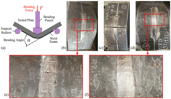
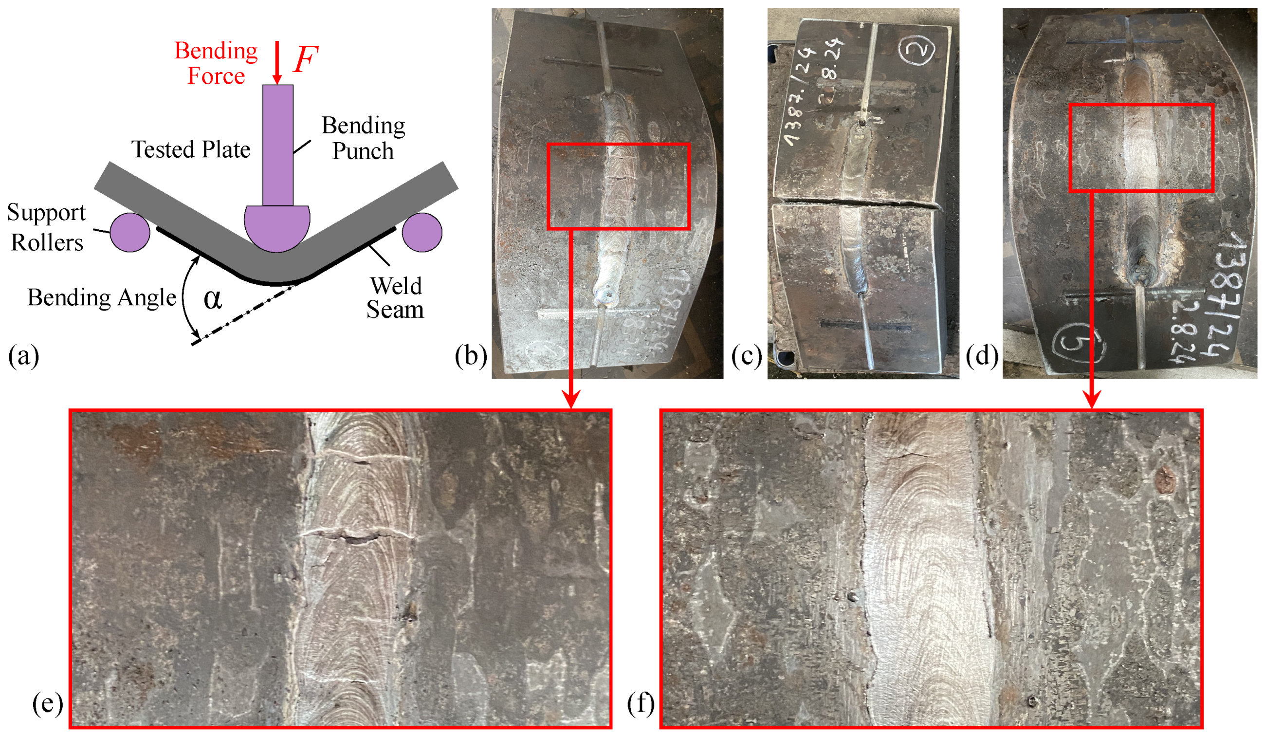
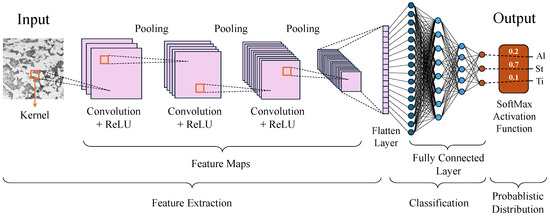
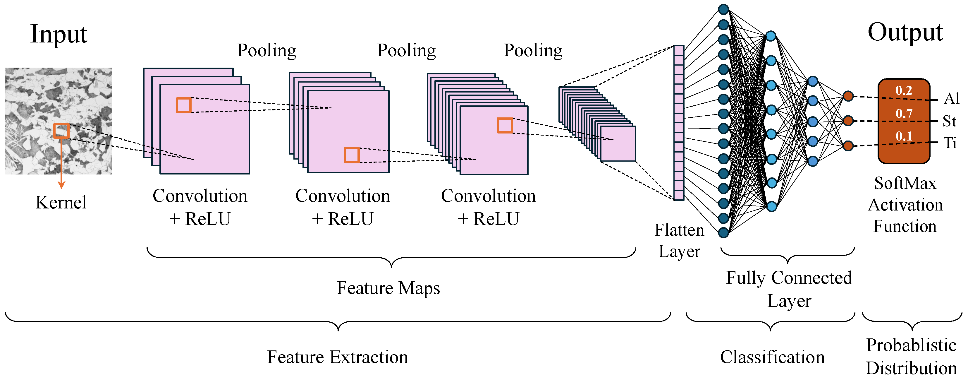
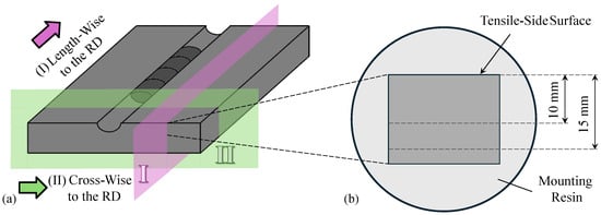
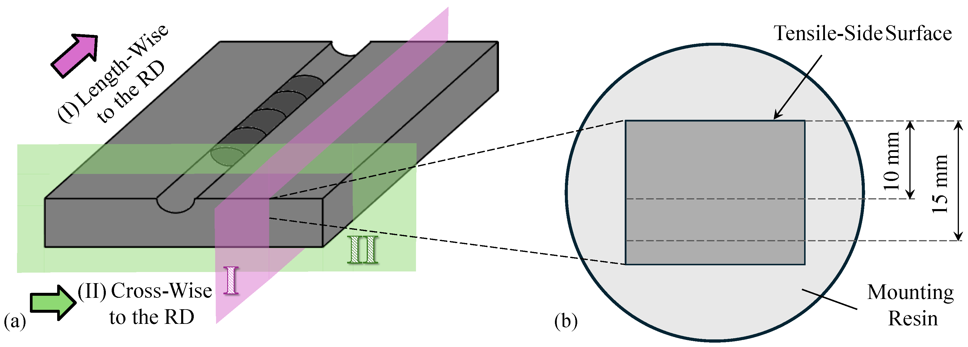
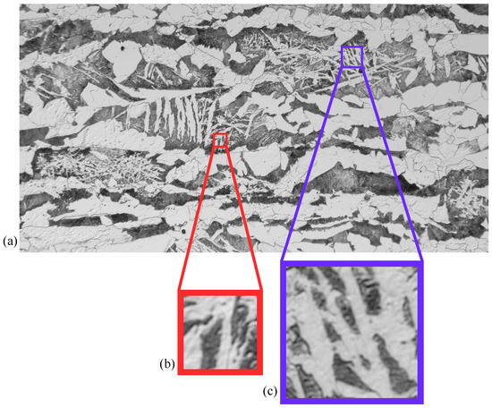
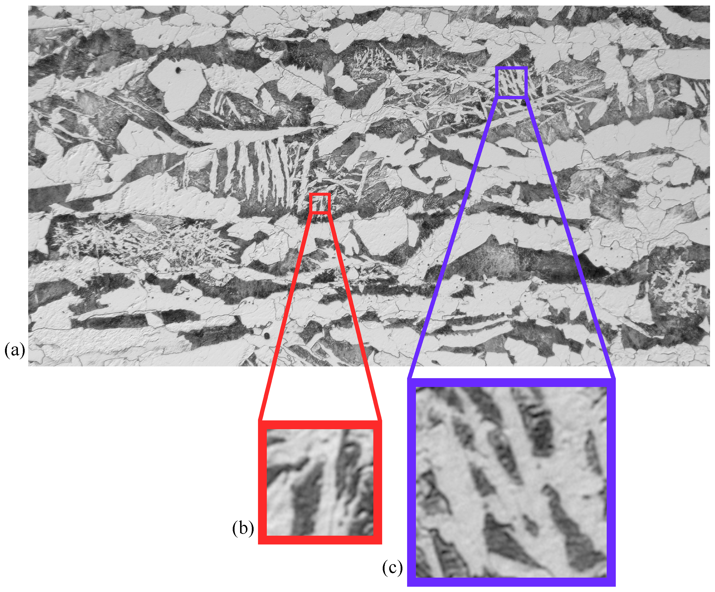
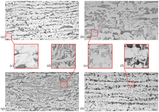
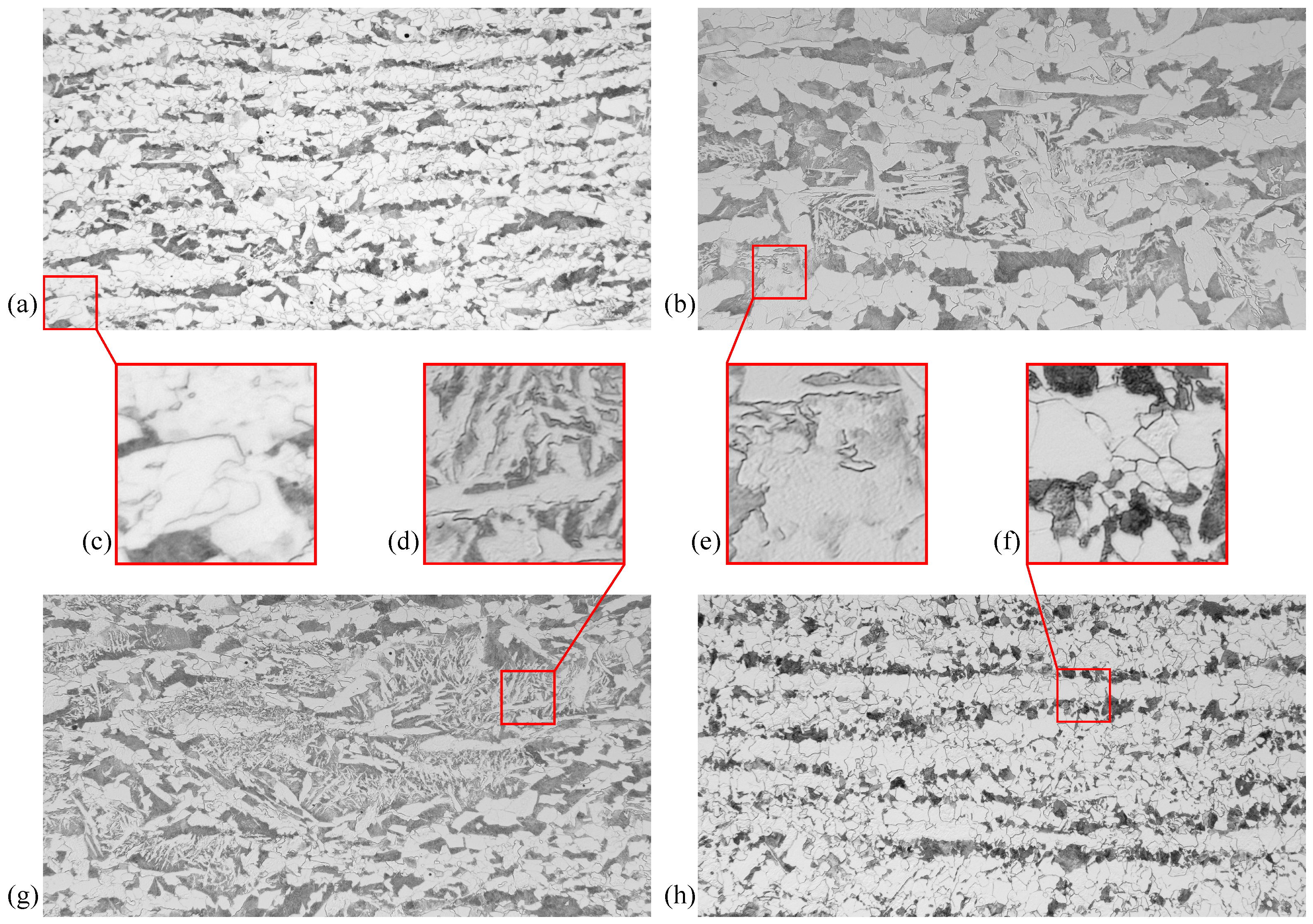
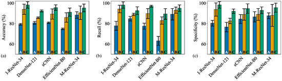
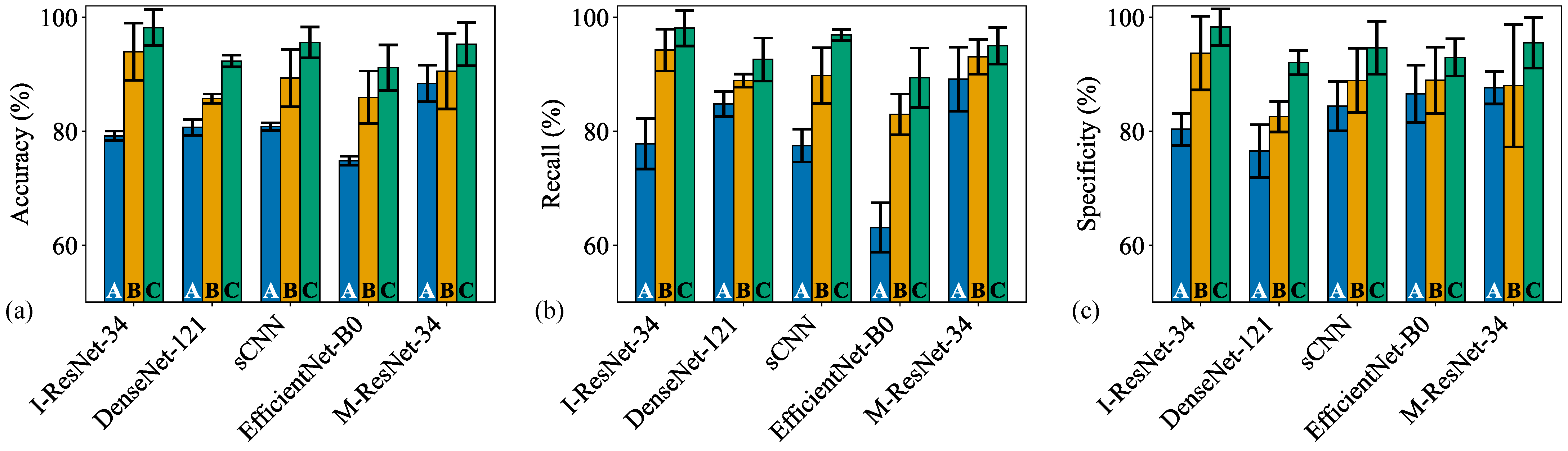
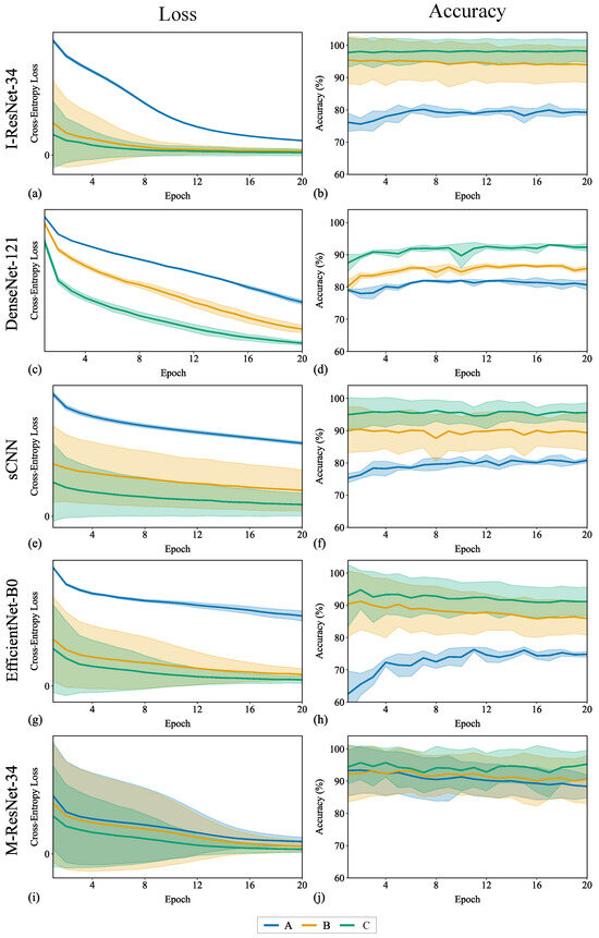
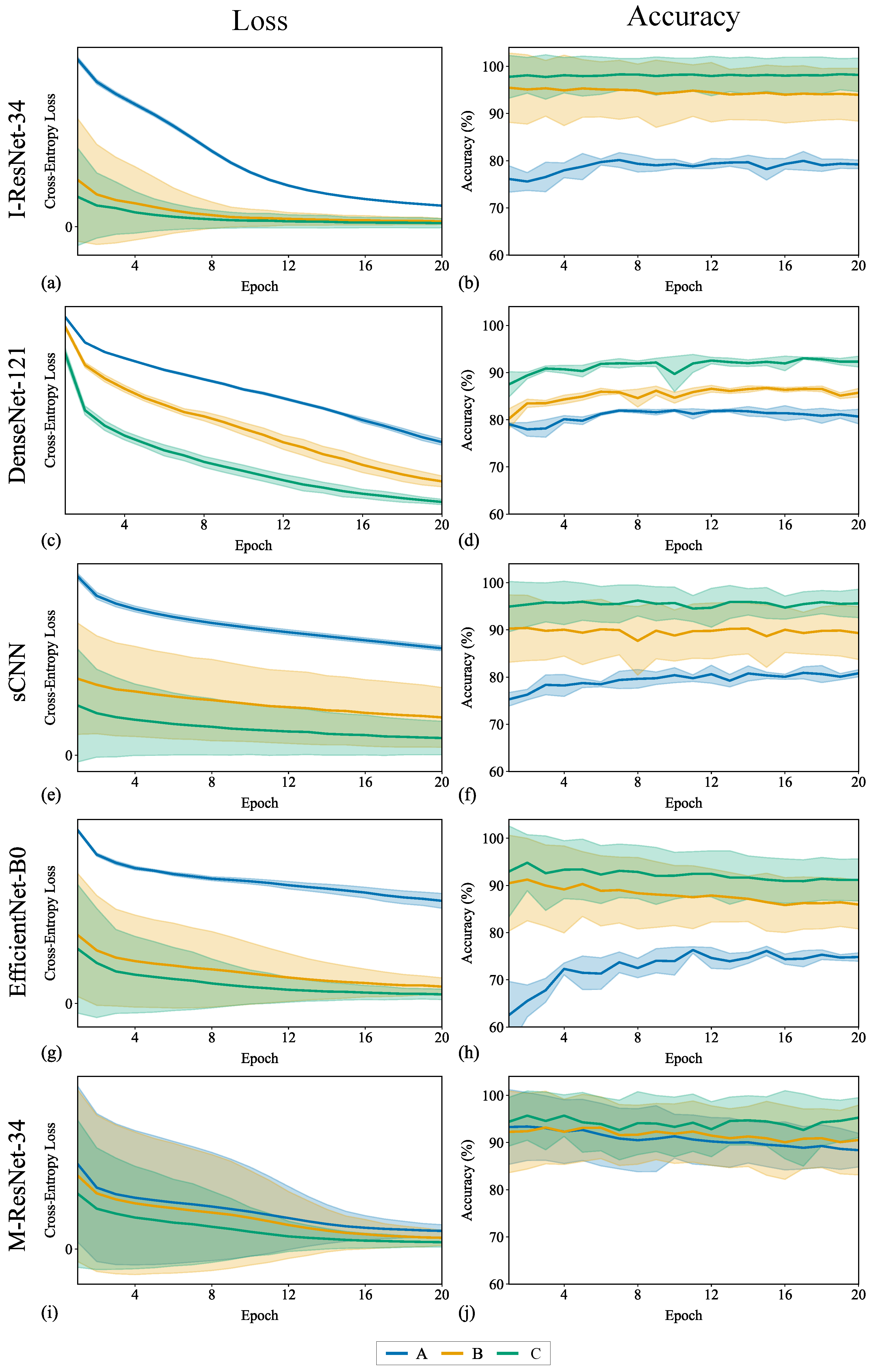
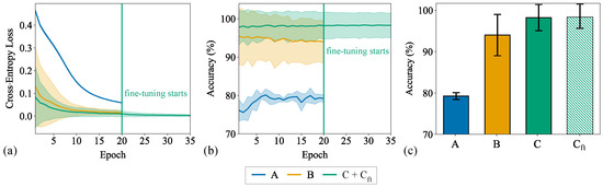
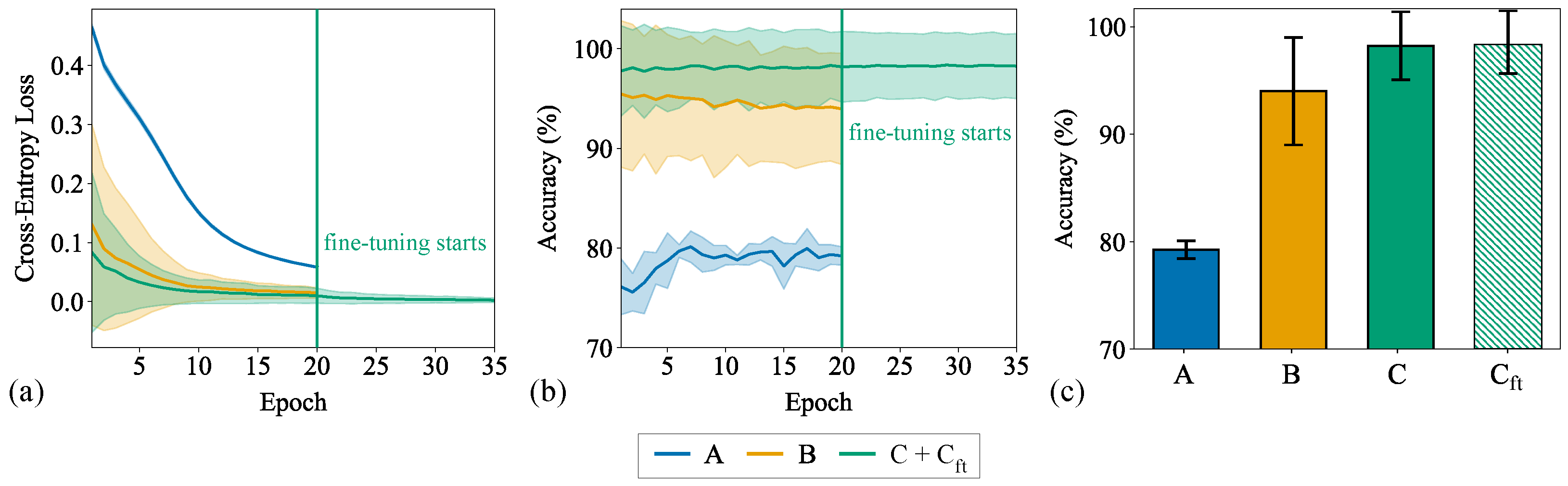
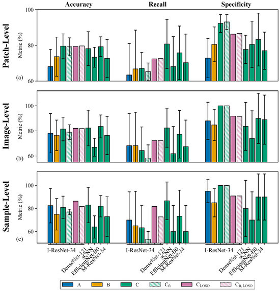
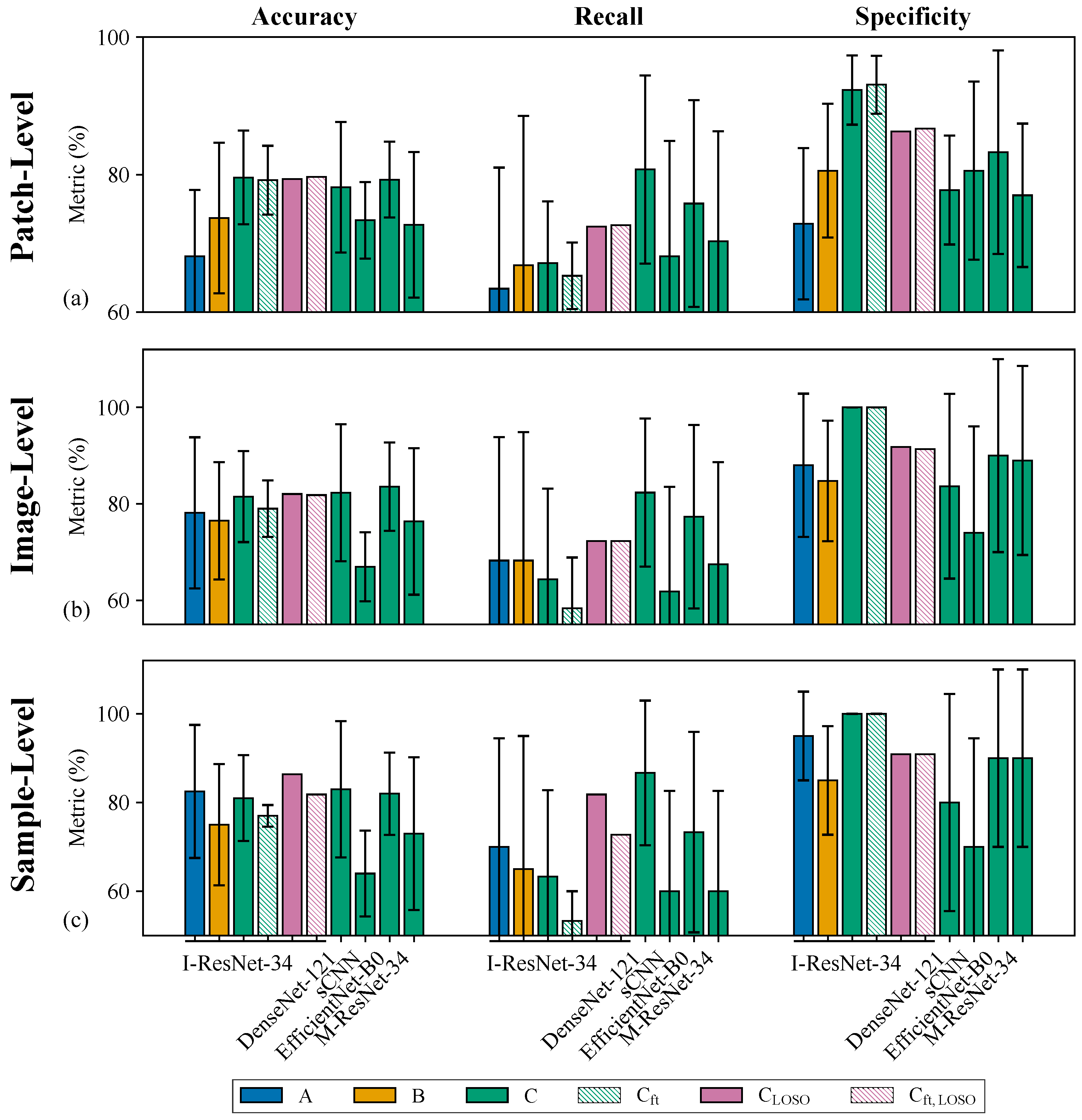
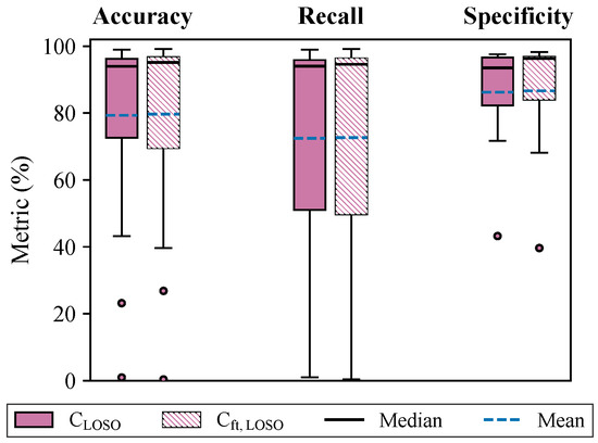
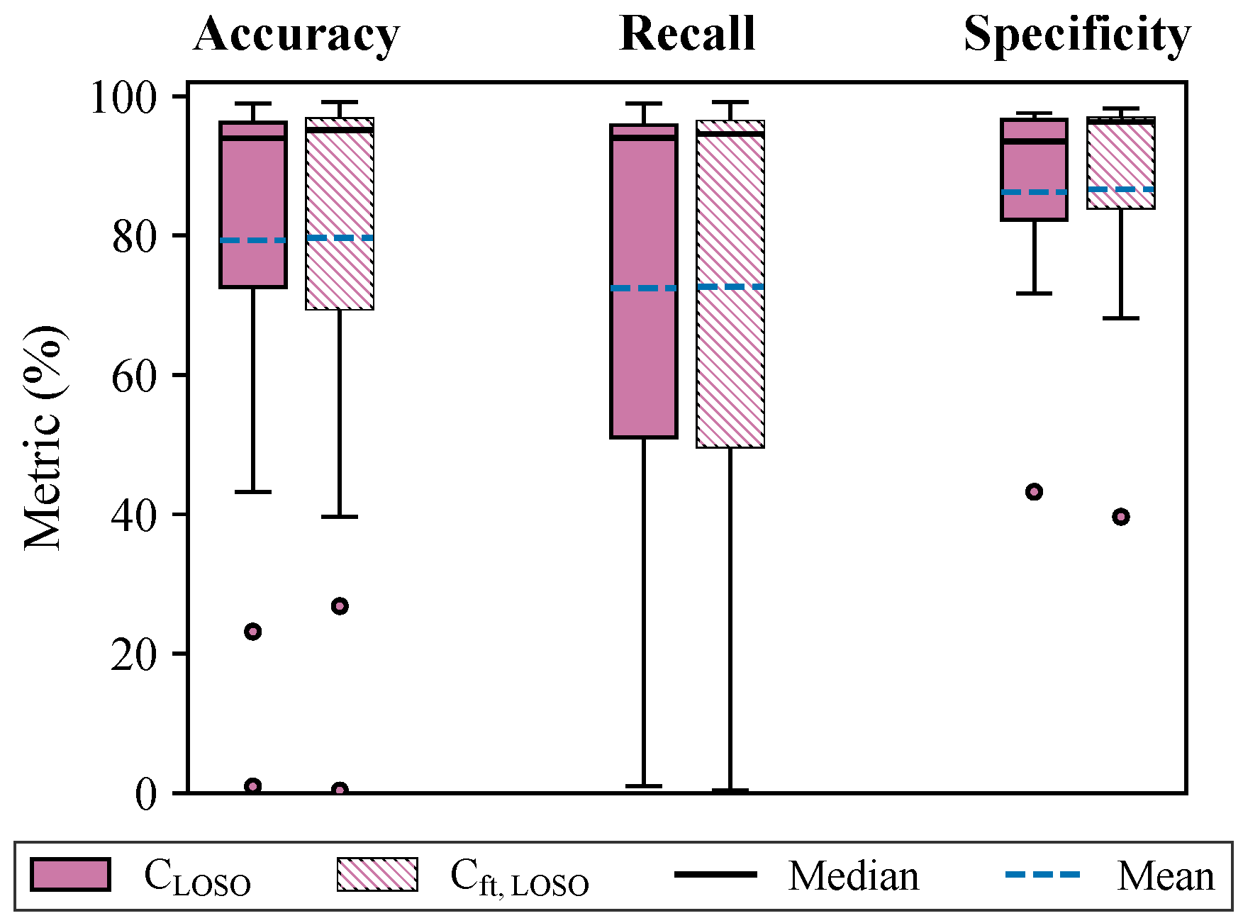
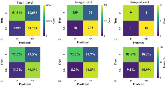
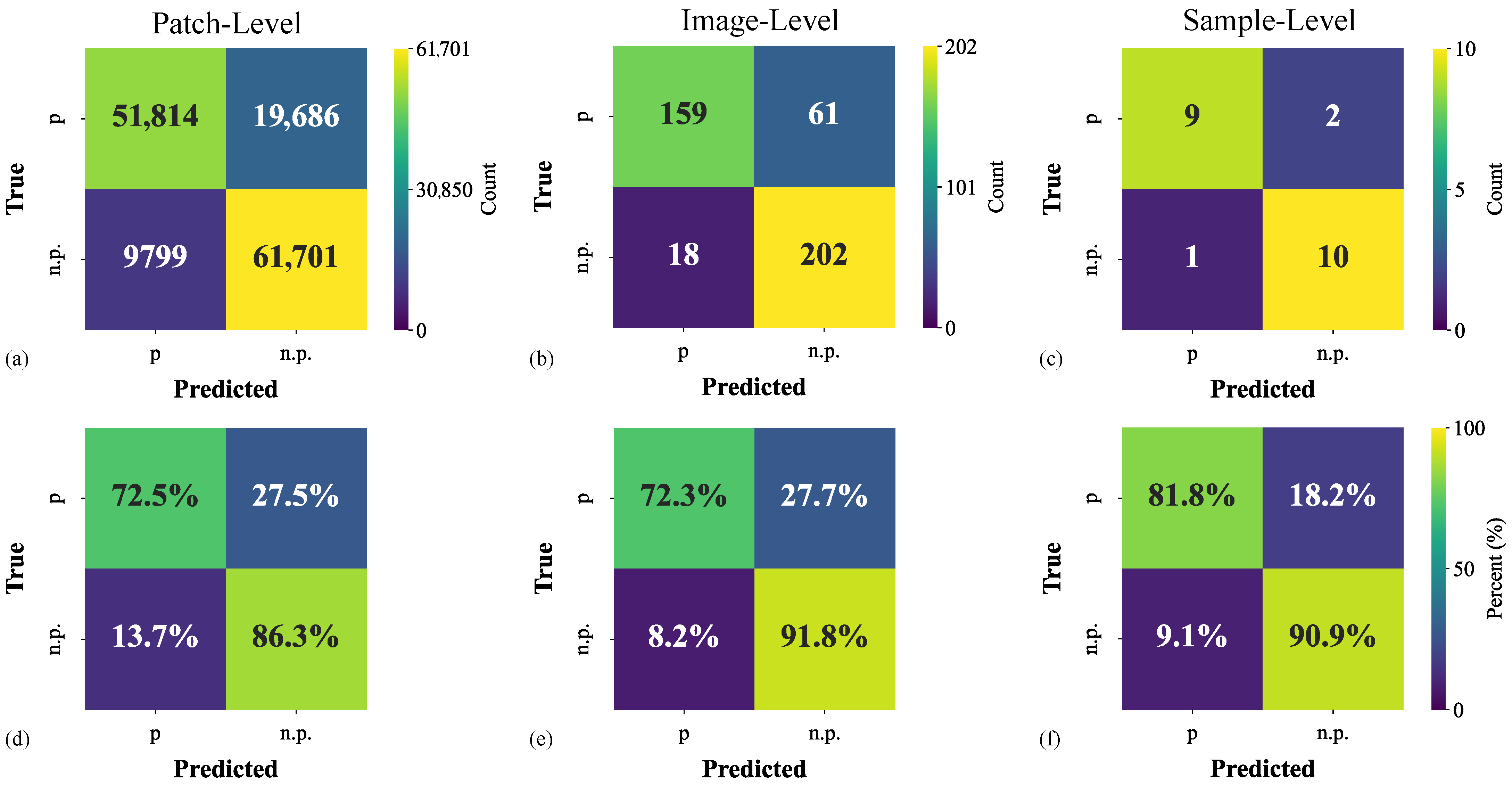
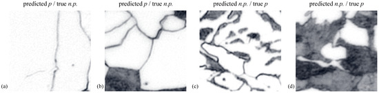
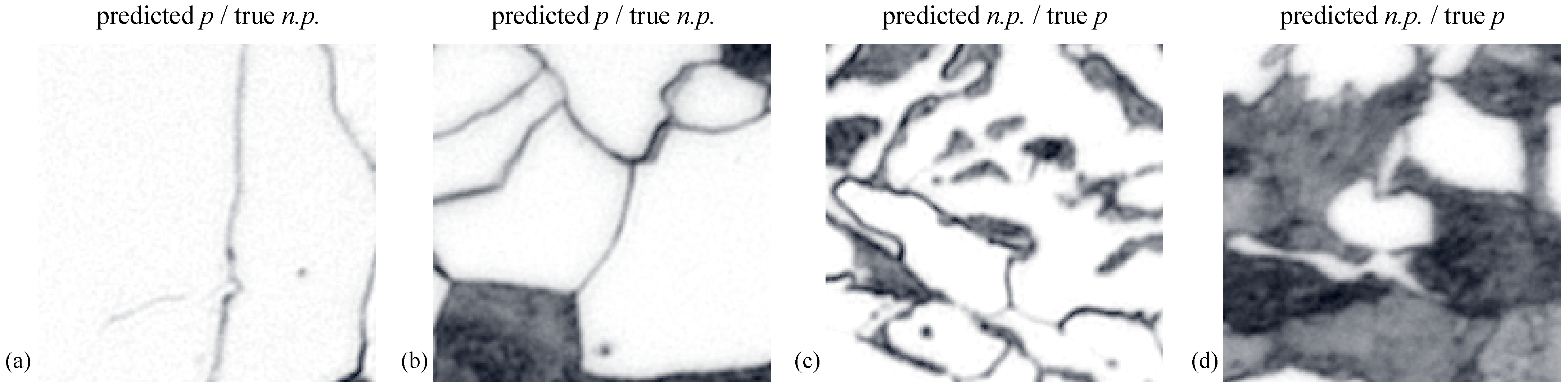
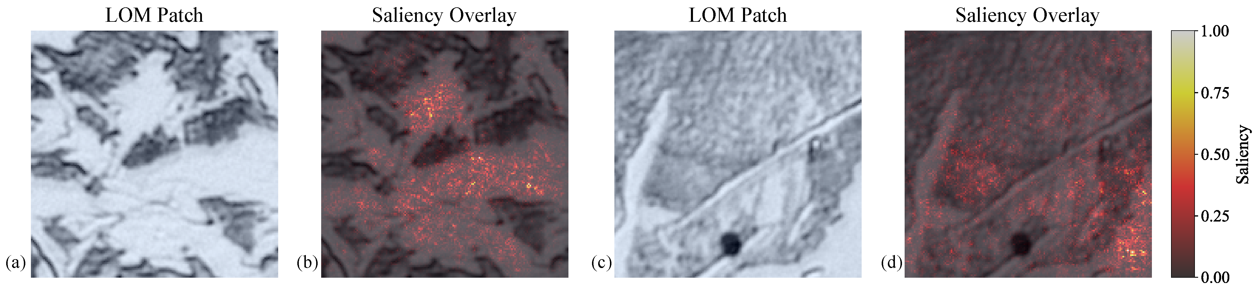

Disclaimer/Publisher’s Note: The statements, opinions and data contained in all publications are solely those of the individual author(s) and contributor(s) and not of MDPI and/or the editor(s). MDPI and/or the editor(s) disclaim responsibility for any injury to people or property resulting from any ideas, methods, instructions or products referred to in the content. |
© 2026 by the authors. Licensee MDPI, Basel, Switzerland. This article is an open access article distributed under the terms and conditions of the Creative Commons Attribution (CC BY) license.