


Abstract
Laser Powder Bed Fusion (PBF-LB) is currently one of the most versatile and adopted additive manufacturing technologies for printing metals. To take new PBF-LB machines into service, a thorough characterization and calibration is often necessary to get the desired output. This is commonly achieved empirically; however, data-driven methods have become more and more available over the last few years. This research explores the use of transfer learning (TL) to transfer process knowledge from an already-established source machine (Nikon SLM 500) to a target machine (Trumpf TruPrint 5000) with different hardware specifications. To predict the tensile properties of AlSi10Mg0.5 utilizing a minimal data set of merely 25 training samples, eight TL model variants, determined by their degrees of training freedom, were investigated. The results showed that TL is effective in transferring machine learning (ML)-based process models. High prediction accuracy was achieved on the target machine, with coefficient of determination () values reaching 75.5% for yield strength, 82.1% for ultimate tensile strength, and up to 92.0% for elongation at break in testing. Additionally, a weighted mean model ensemble of all eight single models was developed, including all eight TL variants, to enable higher prediction robustness. Validation trials for three different use cases confirmed the capability of the approach to optimize processing conditions, like increasing hatch scan speed by 167% to 292% while maintaining high mechanical performance. Additional microstructure analysis was given to support the findings. The results demonstrate a time- and resource-efficient approach for rapid industrialization of PBF-LB machines, combining ML-based process modeling with machine-specific data.
1. Introduction
Laser powder bed fusion (PBF-LB) is at present one of the most established additive manufacturing processes to build metallic near-net-shape structures. It offers a lot of design freedom and flexibility to produce small- to medium-sized parts with minimal tooling effort [1]. However, it also comes with high process complexity, since apart from selecting the right feedstock material for the job, finding the optimal processing parameters can be challenging. Parameters, like preheating temperature [2,3], laser scan speed and power [4], or layer height [5,6], must be optimized to obtain the desired processing results. To find optimal solutions in this multi-dimensional parameter space, data-driven methods and especially machine learning has been discussed as a useful tool by a lot of studies in the last years, e.g., on modeling part density and porosity [7,8,9,10,11,12], functional materials properties [13,14], or mechanical properties like Charpy impact energies [15,16,17] and tensile properties [18,19].
Despite these efforts, another variable represents the PBF-LB machine itself. Every machine has to be characterized and individually tuned in order to deliver the desired results. This might not be an issue for a single-machine setup, yet for an industrialized multi-machine production system, the effort for initial parametrization and ensuring comparable results can scale up rapidly to counteract machine-to-machine variability, reported for example in [20,21,22,23]. The reasons for these variations are multilateral differences in the machine’s technical configuration. It was reported, for example, that different shielding gas flows affect porosity, melt pool geometry, and mechanical properties [24,25,26]. Additional factors are the characteristics of the laser spot, i.e., diameter, focus or caustic [27] and scanning strategies [28], among others. All these influences, or the simple fact that different machines do not offer the same parameter ranges (Table 1), may lead to a different output.
Table 1.
Differences in the parameter ranges between the Nikon SLM Solutions SLM 500 and Trumpf TruPrint 5000 [29,30] used in this research.
Accommodating the above-mentioned advances in process modeling, it seems to be beneficial to use existing process models on new machines (target) and adapt them to the individual machining properties. To achieve this, pre-trained machine learning models can be trained further on data of the target machine to customize them to new or similar situations [31]. According to Tang et al. [32], with this transfer learning (TL) approach, it is possible to generate working process models for a target system in the additive manufacturing domain, while requiring limited amounts of training data. With regard to PBF-LB, TL was used to transfer process knowledge between different PBF-LB printers to predict relative densities with relatively small amounts of training data, ranging between 7 and 49 data vectors on the target machines [33,34]. The material studied was Ti-6Al-4V based on the dataset of Liu et al. [35]. Bahari-Sambran et al. [36] used TL as a tool to investigate processing maps for AlSi10Mg0.5 to optimize relative density. Skiadopoulus et al. [37] pre-trained a neural network on synthetic data of porosity and transferred the model on actual experimental data of printed AlSi10Mg0.5 samples. Lou et al. [38] used process monitoring images during sample printing to predict ultimate tensile strength and elongation at break. To extract relevant features out of 60 process parameter sets, a pre-trained convolutional neural network was used and adapted to the specific task via transfer learning. These examples show the potential of TL in PBF-LB; however, a combination of all aspects—using TL to transfer process models between different machines to predict yield strength, ultimate tensile strength, and elongation at break of AlSi10Mg0.5 utilizing small training datasets—has not been reported yet.
With that background, this research is exploring the application of TL to transfer an existing process model from our Nikon SLM 500 machine (source) onto a Trumpf TruPrint 5000 machine. The pre-trained source models resulted from our previous research [39]. In that study, newly initialized neural networks were exclusively trained on data produced on a Nikon SLM 500 machine. No transfer learning was applied, or external data were used in training. The resulting models for yield strength, ultimate tensile strength, and elongation at break were used in this TL approach.
Both machines cover different parameter ranges, especially in terms of maximum laser power and scan speed or laser beam radius; however, a sufficient overlap of both machines is given. Moreover, it is possible to manipulate the same parameters to control the PBF-LB process. Thus, we explored an inductive transfer learning approach with parameter transfer [31]. We tested the use of a small training dataset to yield usable target models to predict tensile properties of AlSi10Mg0.5 parts, while keeping expensive empirical testing to a minimum. The resulting models for yield strength, ultimate tensile strength, and elongation at break were validated in their performance and tested on three optimization scenarios.
2. Methodology
2.1. Data Creation: Sample Manufacturing and Evaluation
The target PBF-LB machine, for which an existing process model was transferred, was a four-laser TruPrint 5000 by TRUMPF Laser- und Systemtechnik GmbH, Ditzingen, Germany, with a 1064 nm fiber laser and a maximum power of 500 W per laser source [29]. To create the necessary training data on the new PBF-LB machine, the same methodology as described in our previous research on process modeling on an SLM 500 machine by Nikon SLM Solutions AG [39] was utilized. The different parameter ranges for both machines are listed in Table 1.
According to Tang et al. [33], the size ratio of the target to source datasets, given in Equation (1), greatly determines the transfer quality. According to their study, should be between 0.2 and 0.7, better greater than 0.5 to reach a positive transfer. As we used parameter combinations on our source model [39], parameter combinations were chosen as training data for our target dataset. Therefore, the proposed lower limit of was fulfilled.
- —Size of the training dataset on target machine
- —Size of the training dataset on source machine
With the parameter ranges given in Table 2, 25 randomly distributed parameter combinations were determined based on the melt-mode model proposed by Patel et al. [40]. It can be seen in Table 2 how the selected parameter ranges of the target machine overlapped with the training parameters of the source machine to ensure a positive transfer. For each combination, three tensile specimens were assigned. In total, 75 tensile specimens of geometry A4 × 20 according to DIN 50125 were printed with gas-atomized AlSi10Mg0.5 powder, a constant layer thickness of 50 μm, and a constant laser spot diameter of 100 μm. Nitrogen was used as shielding gas.
Table 2.
Variation of PBF-LB parameters for the TruPrint 5000 for the training dataset, actual ranges of the training dataset. The parameter ranges for training the source models from [39] on the Nikon SLM500 [39] are given in brackets for comparison.
For validation, specific parameter combinations were determined by the resulting process models in each use case described in Section 3.5. For every validation parameter set, seven tensile specimens and one density cube (ca. 1 cm × 1 cm × 1 cm) were printed.
The tensile specimens were tested on an AllroundLine Z100 tensile tester including a roboTest L, both made by ZwickRoell GmbH & Co. KG, Ulm, Germany. From the resulting stress–strain curves, the yield strength Rp0.2 (YS), the ultimate tensile strength Rm (UTS), and the elongation at break (A) were evaluated and the mean value of the three samples per parameter combination was used. All three tensile properties served as target values for subsequent machine learning.
The density cubes from the validation trials were used for microstructure evaluation. The specimens were cut perpendicular to the layers, polished, and etched for ca. 30 s with Keller’s reagent (97 mL of distilled water, 1 mL nitric acid (65%), 2 mL hydrochloric acid (37%), 0.5 g of sodium fluoride) to enhance contrast.
The microstructure images were captured both via light-optical microscopy and scanning electron microscopy (SEM). The microscope Polyvar by Reichert-Jung equipped with a digital camera ProgRes SpeedXT core 3 by Jenoptik AG, Jena, Germany and the scanning electron microscope Zeiss GeminiSEM 360 (Carl Zeiss Microscopy GmbH, Jena, Germany) with Oxford Ultim Max 100 EDS (Oxford Instruments plc, Abingdon, UK) detector were used.
2.2. Transfer Learning
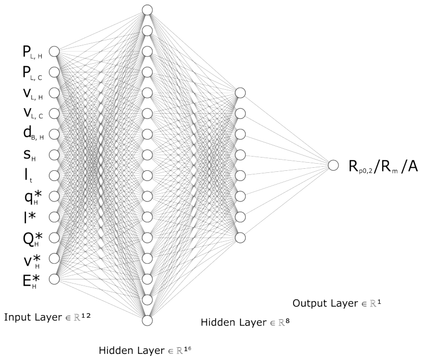
The transfer learning starts with an existing, pre-trained machine learning model that contains process knowledge of a similar domain, i.e., same process parameter dependencies in PBF-LB on different machines. The trained and evaluated models from [39] were used as the source models for this study. These dense neural networks (DNNs) were trained on data from a Nikon SLM 500 (Nikon SLM Solutions AG, Lübeck, Germany, source machine, Figure 1). The model’s architecture, processing parameters, and dimensionless parameters were the same as previously reported. Its architecture consists of 12 input neurons—seven process parameters (laser power PL and laser scan speed for both hatch and outer contour, laser beam diameter dB, hatch distance sH, and layer thickness tL) and five dimensionless parameters (dl. laser power q*, dl. layer thickness , dl. heat input , dl.scan velocity , and dl. energy ). Two hidden layers of 16 and 8 neurons follow respectively and a single target as output. For each target value (YS, UTS, A), a separate model was trained, and therefore, the transfer was based on these three models.
The models were implemented in Python 3.9 with Pytorch 2.3 [41]. All training and testing of the ML models was performed on common desktop hardware, specifically an Elitebook 850G8 by HP with a quad core Intel Core i7-1165G7 processor, 16 GB RAM, and an additional NVIDIA GeForce MX450 N18S-G5 graphics card with 2 GB VRAM to speed up training.
Figure 1.
Dense neural network architecture used for transfer learning [39], created with NN-SVG [42].
In order to transfer the model, the pre-trained DNN from [39] was trained further with new data from the TruPrint 5000 machine. Since similar dependencies between process parameters (input) and tensile properties (output) on the TruPrint 5000 were expected, compared with the Nikon SLM500, the aforementioned amount of training data was used. Thus, the highest reduction in physical trials to yield a suitable process model was to be achieved.
For the approaches regarding transfer learning, it was mainly focused on those that keep certain layers of the neural network on the pre-trained level (i.e., “fixed”) and let the remaining ones adapt their weights and biases to the new data during training [43]. This adds the theoretical benefit that it decreases the network’s complexity, reducing the chance of overfitting the small dataset that was used for training. The batch normalization parameters were never fixed. Since it is not trivial, which layers to fix and which to train, different levels of constraints were tested. First, one of three layers were opened; second, two layers; and finally, all three layers were opened for further training. Additionally, newly initialized models were used as well as a newly initialized model as a baseline comparison. The neural network’s trainable parameters can be calculated by , where n are the numbers of input parameters, m is the number of outputs per layer, and +1 accounts for the bias [44,45]. With that, for the network used in this study, it can be derived that the first layer has 208 trainable parameters, the second layer 136, and the third layer 9 trainable parameters. Depending on how many layers are fixed or trainable, the degree of training freedom can be given. The resulting model variants and their designations were the following:
- 1.
- Model variants with one trainable layer.
- First layer trainable (FLT)—208 trainable parameters.
- Second layer trainable (SLT)—136 trainable parameters.
- Last layer trainable (LLT)—9 trainable parameters.
- 2.
- Model variants with two trainable layers.
- First layer fixed (FLF)—145 trainable parameters.
- Second layer fixed (SLF)—217 trainable parameters.
- Last layer fixed (LLF)—344 trainable parameters.
- 3.
- Model variants without constraint.
- Full model trainable (FMT)—353 trainable parameters.
- Newly initialized model (NM)—353 trainable parameters.
Additionally, to find the optimal hyperparameters for each model variant, a grid search was performed (see Table 3). The resulting hyperparameters for each model variant and target value are given in Table A1, Table A2 and Table A3 in Appendix A.
Table 3.
Hyperparameter ranges for grid search.
Consistent with our prior research, the error metrics mean absolute error MAE (Equation (2)) and coefficient of determination (Equation (3)) were used to analyze and compare the performance of the given model variants for both grid search and prediction performance [39,46,47]. K-fold cross-validation was used for all training and testing, utilizing four folds with each with a constant seed for model comparison.
- N—Size of the dataset.
- —Actual target value for the i-th data sample.
- —Predicted output for the i-th data sample.
- N—Size of the dataset.
- —Actual target value for the i-th data sample.
- —Predicted output for the i-th data sample.
- —Mean value of all target values in the dataset.
3. Transfer Learning Results, Validation, and Discussion
To evaluate the TL-performance of the model variants, first, the models’ fits for testing and MAE were compared against each other. Second, the training scores were taken into consideration with respect to the difference between training, testing, and overfitting.
3.1. Yield Strength
The resulting metrics of the different TL models for yield strength prediction are displayed in Table 4 and Table 5. The FMT models yielded the highest average of 75.5% and an average MAEtest,FMT of 11.8 MPa. Following that, the FLT model with % (MAEtest,FLT = 13.3 MPa), NM with % ( = 11.6 MPa), and SLF with % ( = 11.8 MPa) scored a relatively high models’ fit and low mean errors. Taking the training values into account, the SLF model showed the least difference between testing and training (%, MPa) with a slight overfitting due to the higher training score. The FMT model exhibited weaker training performance with % and = 16.0 MPa, as well as the FLT and NM models. The newly initialized model NM yielded the second lowest training performance, in front of the SLT model, which was the lowest-performing model variant for yield strength prediction. All other models (SLT, LLT, FLF and LLF) scored below 50% or showed negative scores in one or more folds and might be considered unsuitable for the task.
Table 4.
cross-validation test results for yield strength using the averaged Trumpf dataset; results for each fold and its average are given as well as average training values for comparison.
Table 5.
MAE [MPa] cross-validation test results for yield strength using the averaged Trumpf dataset; results for each fold and its average are given as well as average training values for comparison.
Regarding the degrees of freedom, the results show that leaving the first layer trainable has a positive impact on the model transfer. From the models with one trainable layer, the FLT model scored the highest, whereas in the second layer, the lowest models fit. The second layer also seemed to impact the models with two trainable layers the least, and combining the first and last layers trainable yielded the highest model fit. Increasing the degrees of freedom further to fully trainable models, the test scores became better, yet also the errors increased. Thus, the most stable TL model for yield strength in this trial was the Second Layer Fixed (SLF). The slight overfit of the SLF model must be considered when selecting this model.
3.2. Ultimate Tensile Strength
Based on Table 6, the best model fit for UTS prediction was attained by the FLF model with , and with 81.1% the LLT came second. Both models also scored the lowest mean errors (Table 7) of = 14.4 MPa and = 18.2 MPa, respectively. The SLT and FLT models followed with and . The mean error of the SLT model was increased with = 22.3 MPa, whereas the SLT error was comparable ( = 18.9 MPa) to the LLT model despite its lower R2 value. The NM and the SLF showed the highest and, therefore, worst MAEtest of 24.7 and 22.5 MPa. This coincided with the lowest values (48.7% and 41.0%), so these two models can be assumed to perform worst.
Table 6.
cross-validation test results for ultimate tensile strength using the averaged Trumpf dataset; results for each fold and its average are given as well as average training values for comparison.
Table 7.
MAE [MPa] cross-validation test results for ultimate tensile strength using the averaged Trumpf dataset; results for each fold and their average is given as well as average training values for comparison.
Investigating the differences between train and test results, the higher compared with the values for the SLF, LLF, FMT, and NM models showed signs of overfitting. The between testing and training up to 33% for SLF showed that the mentioned approaches are strongly overfitting on the training data while performing significantly worse on the test samples. In addition to that, the SLF, LLF, and NM models experienced negative values in fold 2; thus, their reliability seems questionable.
The FLF model, which performed best in testing, showed the second lowest model fit in training with 57.8% before the NM with 54.1%. This does not indicate overfitting; however, it is also not an indicator for robustness of the model. In this regard, the FLT, SLT, or LLT models seemed more reliable.
The good results of the SLT or LLT, in combination with the scores for the FLF, may indicate that these models benefit from further training the second and last layers. This is evident from the fact that, among all three models with one trainable layer, the performance increases when the second or third layer is trainable, i.e., with reduced trainable parameters. Additionally, with two trainable layers, the best performance can be observed with the second and third layer trainable, as the FLF model represented.
3.3. Elongation at Break
Overall, the average shown in Table 8 ranges from 66.4% to 92.0% with one exception being the NM, which can be explained by the significantly poor performance on folds 1 and 2 that yield the highly negative score. The same can be seen in Table 9 with MAEtest results of 0.559% to 0.267% elongation. The three best models concerning the average were, in descending order, the LLF (92.0%), the FLF (87.9%), and the FMT (87.6%). They also shared the three best , although the second best was the FMT with an error of 0.302%, beating the 0.304% of the FLF. The LLF was the best with 0.267%. The newly initialized model NM was not able to learn the underlying pattern or structure of the data, as the negative and MAE values of folds 1 and 2 show. This indicates that the amount of training data is not sufficient to yield a usable process model for elongation at break without pre-training. The second-lowest-performing model was FLT with = 66.4%, which also showed a comparably high of 0.559%. All models with one trainable layer and the SLF model showed larger than , with a max delta of 8.6% in the case of the LLT model, indicating overfitting. Despite having the highest level of trainable parameters, the first layer seemed to have the least influence of all models with one trainable layer. In contrast, the SLF had the lowest average of 72.0% of the models with two trainable layers, whereas the FLF and LLF models performed notably better in comparison. The corresponding MAEs supported these observations.
Table 8.
cross-validation test results for elongation at break using the averaged Trumpf dataset; results for each fold and its average are given as well as average training values for comparison.
Table 9.
MAE [%] cross-validation test results for elongation at break using the averaged Trumpf dataset; results for each fold and its average are given as well as average training values for comparison.
The good choice for the predictions was the LLF model, FLF, or FMT. On fold 3, the LLF and FMT were the models with the best (test) of 96.2% and 96.9%, while the FLF performed best on fold 1 with 94.7% (test). Additionally, all three models showed no signs of overfitting.
3.4. Weighted Mean Model
The results showed that the transfer of the initial pre-trained model to the domain of the new PBF-LB machine was possible. For all three target values, reasonable TL models can be found, considering high -values for testing and training, low overfitting during training and low errors. Moreover, the approach to test the different trainable layers and degrees of freedom seemed beneficial, since it was not obvious which variant was to perform best. The yield strength, for example, was predicted best, when the first and third layers were trainable, whereas, for UTS, the second and third layers and, for elongation, the first and second layers were most beneficial. Apart from that, many other variants were also not far off and delivered decent results, especially when the individual folds are taken into account. Overall, the results present a non-trivial situation on how to decide for the best and most robust model for exploitation in subsequent validation trials.
As it will be demonstrated in the following validation section, the single models can lack robustness for an actual use case; thus, it is proposed to use all variants in a custom ensemble. The ensemble model—designated as the weighted mean model (WM)—uses a weighted mean of the prediction of every model variant, as Equation (4) states. The specific -value of the used model state serves as the weight factor, and the fold with the highest testing scores was used. Using the highest scoring folds enabled the WM model to include every model variant and ensured that only positive scores were included. It is pointed out, at this stage, that this approach induced a certain bias to the WM model. Thus, its performance may be considered an upper-boundary estimate in this study. Different approaches to further improve WM models are indicated in the outlook; see Section 4. The respective -value for the resulting WM model was calculated according to Equation (5).
As the -values, which serve as weights, do not add up to 1, it is not sufficient to just add the predictions of all models without any normalization since then the prediction of the weighted mean model would be in a different value range. Specifically, if all models would have the same prediction and the sum of the -values is 2, for example, the prediction would be doubled. Therefore, a normalization is needed, which can be seen in Equation (4), where the weighted sum of predictions from the model was divided by the sum of all -values to get the actual correct value range of the original predictions. The same applies for the calculation of the weighted (Equation (5)), which also has to be normalized in order to get the correct outcome.
- —-value of the i-th model variant of the best fold from testing, serves as the weight factor.
- —prediction (output) of the i-th model variant, with the best fold from testing.
- —-value of the i-th model variant of the best fold from testing, serves as the weight factor.
The resulting weighted mean model was used in the validation trials and was compared with the single model’s performance.
3.5. Model Validation on Specific Use Cases
To validate the resulting models, three use cases based on real-world optimization scenarios were designed. In parameter development, optimizing strength, ductility, or productivity can be of interest. High tensile strength of the printed part allows for better part performance or sleeker designs, whereas increased ductility might be necessary for mechanical fastening, like punch riveting, which requires increased deformation of the material. Maximizing productivity reduces the cost of production and thus enables a broader range of application of printed parts. Although it might be valid to pursue a combination of these optimization goals, for the sake of this study, these targets were used individually to validate the resulting TL models. The general approach for selecting a model was based on the -values during training and testing. As the models were optimized over a wide area of feasible parameters, it was not solely relied on a good but also qualitatively on the predicted response surface within the extended melt mode diagram for hatch parameters. This evaluation was carried out qualitatively by comparing the optimized parameters for a given use case with the contour plot of the predicted response. The goal was to maximize the respective target values while avoiding steep gradients (e.g., Figure A1, lower right corner), or other inconsistencies like kinked contour lines (e.g., Figure A4, around , = 0.9–1.0). Quantitative thresholds for gradients were not used in these trials. This explains why the models that were chosen for the validation are not always the ones with the highest -values. In general, the best fold was used for each selected model. Additionally, for every use case, parameters were optimized using the weighted mean model.
In the process of validation, the focus was on the hatch parameters. Since the outer contour contribution to the sample’s cross section was comparatively low, it was kept constant. The reason for this approach was that the melt-mode model by Patel et al. [40] treats each parameter subset, i.e., either hatch or contour parameters, independently. Thus, keeping the contour parameter constant, the validation could be focused on the hatch parameter optimization, which attributes to the bulk of each sample and thus is presumed to influence the mechanical properties the most. Rather than the mean values of Table 2, a previously known, well-performing productive parameter (PL,C = 410 W, = 750 mm/s) was used for the outer contour to reduce possible negative influences on the samples, e.g., due to contour porosity. Even though this choice may have induced some bias in the system, the hatch optimization was still independent of the contour parameters, and the results can be expected to show valid optimization effects. Moreover, the effects of hatch optimization were clearly distinguishable without the influence of varying contour parameters.
3.5.1. Maximizing Yield and Tensile Strength
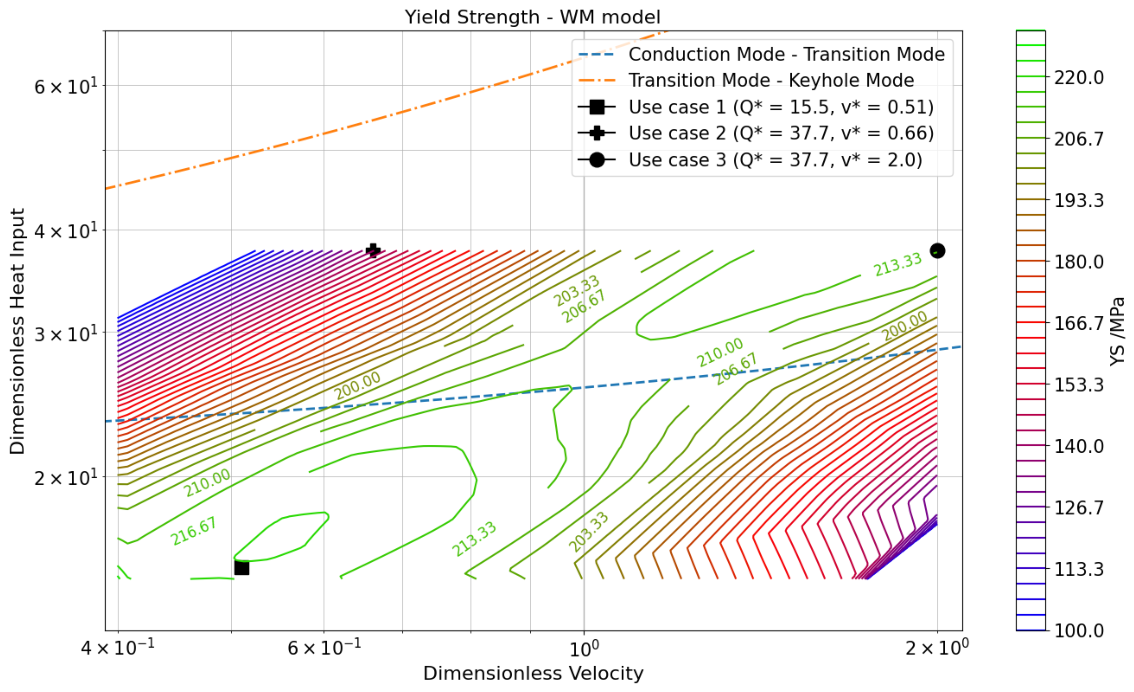
In the first instance, the task was to maximize yield and tensile strength. As previously explained, the models for the parameter selection were chosen based first on -values and second on the characteristics of the predicted response surface (Figure 2 and Appendix B). Thresholds for both yield and tensile strength were set that guaranteed an overlap for the areas of feasible parameters with target values higher than the chosen properties. Then, the predictions were matched such that a list of parameters with their corresponding outcomes was generated. The list was sorted in descending order for both strength measures, and then a parameter set was selected representing the point where increasing one value would result in a decrease in the other. As a result, the SLF model for yield strength and FLT model for the tensile strength were chosen for validation.
Figure 2.
Predicted response surface for yield strength by WM model; parameter points for use case 1 (maximizing yield and tensile strength), use case 2 (maximizing ductility), and use case 3 (maximizing productivity) are given.
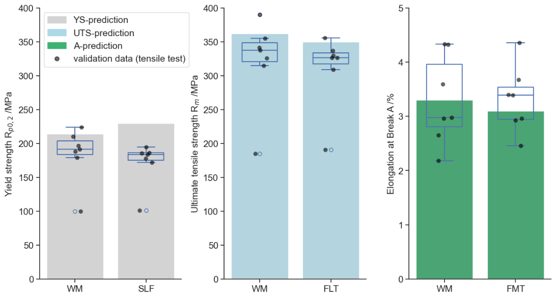
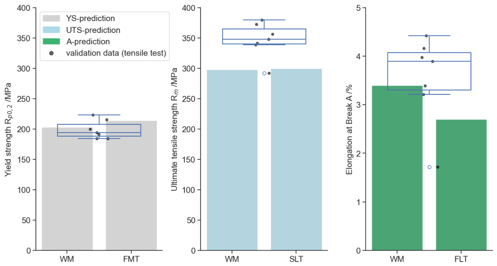
The corresponding dimensionless parameters, complementing predictions for the respective target values and actual validation values are given in Table 10. Additionally, predictions and validation values are compared in Figure 3. The results showed that the validation properties did not reach the predicted level across all models. Beginning with yield strength, the WM model predicted MPa, and the validation came to a mean value of Rp0.2,val = (184 ± 37.2) MPa. The SLF model’s prognosis of = 230 MPa was higher than the WM model, and the resulting validation data slightly lower with Rp0.2,val = (172 ± 29.4) MPa. The graph reveals small spread with one obvious outlier around 100 MPa for both the WM and single models. Its low mechanical strength does impact the performance of the validation yield strength negatively. Without that outlier, the results would have been much nearer to the predictions.
Table 10.
Target values for prediction and actual validation trials for maximizing tensile strength, using the single models vs. WM model; with median value , mean value , and standard deviation for validation test data and the respective target values.
Figure 3.
Prediction and validation results for strength optimization; WM model vs. single models: SLF for YS, FLT for UTS, FMT for elongation.
The validation results for ultimate tensile strength appeared similar, as real values were slightly below the prognosis including the negative influence of one low outlier each. The WM model, forecasted at = 362 MPa, came to Rm,val = (321 ± 59.9) MPa. The FLT predicted a UTS of = 350 MPa, and the validation samples reached Rm,val = (311 ± 50.7) MPa.
Considering elongation at break, although not the specific optimization target in this use case, the validation data were quite accurate for both models. The WM model was on target with %; the FMT validation was slightly higher than its forecast of % with %. The elongation showed a much more pronounced spread of the actual values, as expected for this target.
In conclusion, the optimization of yield and tensile strength using the transfer models seemed reasonable. The validation trials for both the WM and single models delivered moderately lower YS and UTS values as predicted, and the elongation values both for validation and prediction matched quite well within their uncertainty. In order to evaluate the spread of the strength values, more data need to be gathered in a second verification lap to either affirm or dismiss the validity of the outlier.
3.5.2. Maximizing Ductility
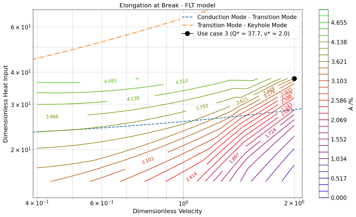
Second, the models were used to maximize the ductility, i.e., elongation at break, of the material. This tensile property had to be maximized separately as it reached its maximum in a different area of print parameters compared with the yield and tensile strength (compare Figure 2, Figure A1 and Figure A2).
For this optimization, only the models that predict the elongation at break and specifically the FMT model with all layers trainable to determine the best parameters as well as the weighted mean model were used. Here, the values had to be maximized based on one prediction, so the predictions could be sorted in descending order and pick the highest one for both models. The resulting parameters were additionally used to predict YS and UTS with their SLF and FLT models, respectively.
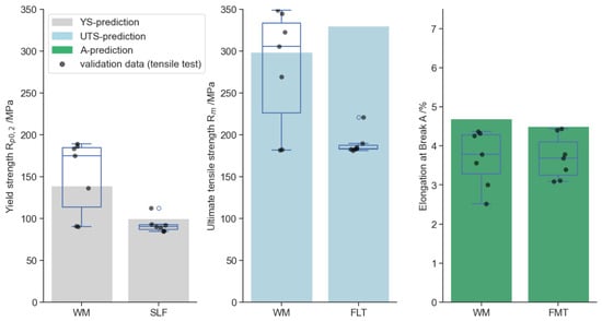
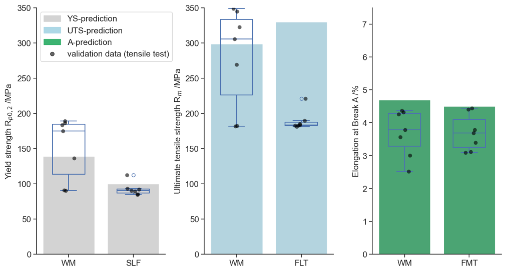
The resulting values for elongation at break and their corresponding strength values are given in Table 11 and presented in Figure 4. The WM model predicted an elongation of %, which the real values with Aval = (3.7 ± 0.7)% did not match. The FMT forecast slightly lower with %, and the resulting elongation came to Aval = (3.7 ± 0.5)%.
Table 11.
Target values for prediction and actual validation trials for maximizing elongation, using the single models vs. WM model; with median value , mean value , and standard deviation for validation test data and the respective target values.
Figure 4.
Prediction and validation results for ductility optimization; WM model vs. single models: SLF for YS, FLT for UTS, FMT for elongation.
With the parameter shifted to the maximum of elongation, the strength values were expected to decrease, since their modeled maxima were located differently. The results reflect that for both models; e.g., the yield strength for the WM model came down to MPa compared with the prediction of the first use case (Section 3.5.1). Its actual value is slightly higher with Rp0.2,val = (150 ± 41.0) MPa, however, still significantly reduced. The prediction of the FLT model for UTS with MPa failed, as it was much higher than the validation trials delivered with Rm,val = (189 ± 13.0) MPa. Overall, the optimization of elongation at break did not exceed the values by much compared with the prior use case. Given the reduced YS and UTS, the resulting elongation was expected to be higher. The subsequent microstructure analysis (see Section 3.5.4) might yield further insights to the shown materials behavior.
3.5.3. Maximizing Productivity
In the third use case, the models were used to increase productivity, i.e., reducing printing time. To achieve this, printing speed was enhanced by maximizing the dimensionless scan velocity and dimensionless heat input to compensate while retaining defined mechanical properties.
As a baseline for this optimization, the results were compared with the prior two use cases, since, in this case, the optimized parameters had to account for all three target properties simultaneously. Both the WM model and single models were compared on one set of samples. The dl. heat input was on the upper maximum of the prediction range with as a result of these conditions, and it was possible to increase the dl. velocity to and laser scan velocity mm/s Table 12. For the single models, the FMT model was used for YS, the SLT model for UTS, and the FLT model for elongation.
Table 12.
Target values for prediction and actual validation trials for maximizing productivity, using the WM and single models on the same parameter; with median value , mean value , and standard deviation for validation test data and the respective target values.
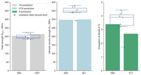
In Figure 5, the predictions and results are shown. It is evident that both the WM and single models delivered largely similar predictions. YS was predicted higher by the WM model ( MPa) compared with the FMT model ( MPa). For elongation, it was the other way around—the WM model predicted lower with % than the FLT model with %.
Figure 5.
Prediction and validation results for productivity optimization; single models: FMT for YS, SLT for UTS, FLT for elongation.
For yield strength, the validation values came down to MPa, which matched both models within its standard deviation. UTS actually was significantly higher with its validation values of MPa than predicted. The elongation at break validation yielded %, which matched with the FLT prediction. The WM model’s forecast, however, was too low.
The productivity increase can be calculated by dividing the increase in scan velocity by the reference velocity: , with , being the laser scan velocity after optimization and the reference scan velocity. Compared with the hatch scan speeds from the first use case (WM model: 589 mm/s, single models: 867 mm/s), an increase in hatch scan speed by 167% to 292%, and for the second use case (WM model: 762 mm/s, single models: 681 mm/s), an increase by 203% to 239% was reached. If the results were compared against the first use case, the mechanical properties with the productive parameter were superior to the max. strength samples. YS was 7.6%, UTS 8.1%, and elongation 6% higher than the validation values for the WM model. The high-productivity parameter was also comparable to the max. elongation results for both the WM and single models. Its value of % was just 0.2% below the max. elongation results, while retaining higher YS and UTS values.
3.5.4. Microstructure Evaluation
As the validation results revealed, the optimization targets can be reached with the available TL models. However, it is a question why the models delivered predominantly higher predictions than the validation trials. Additionally, the different use cases showed partially similar mechanical properties for different process conditions. To further investigate these findings, the microstructure was evaluated.
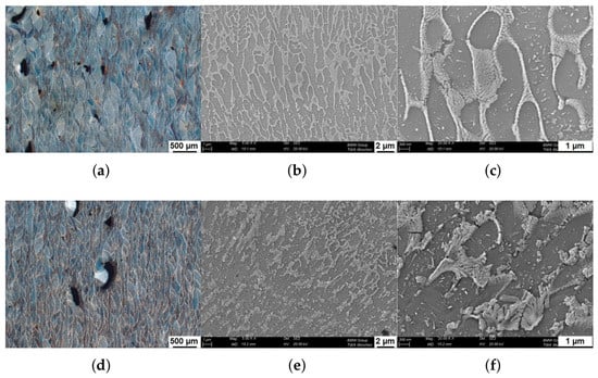
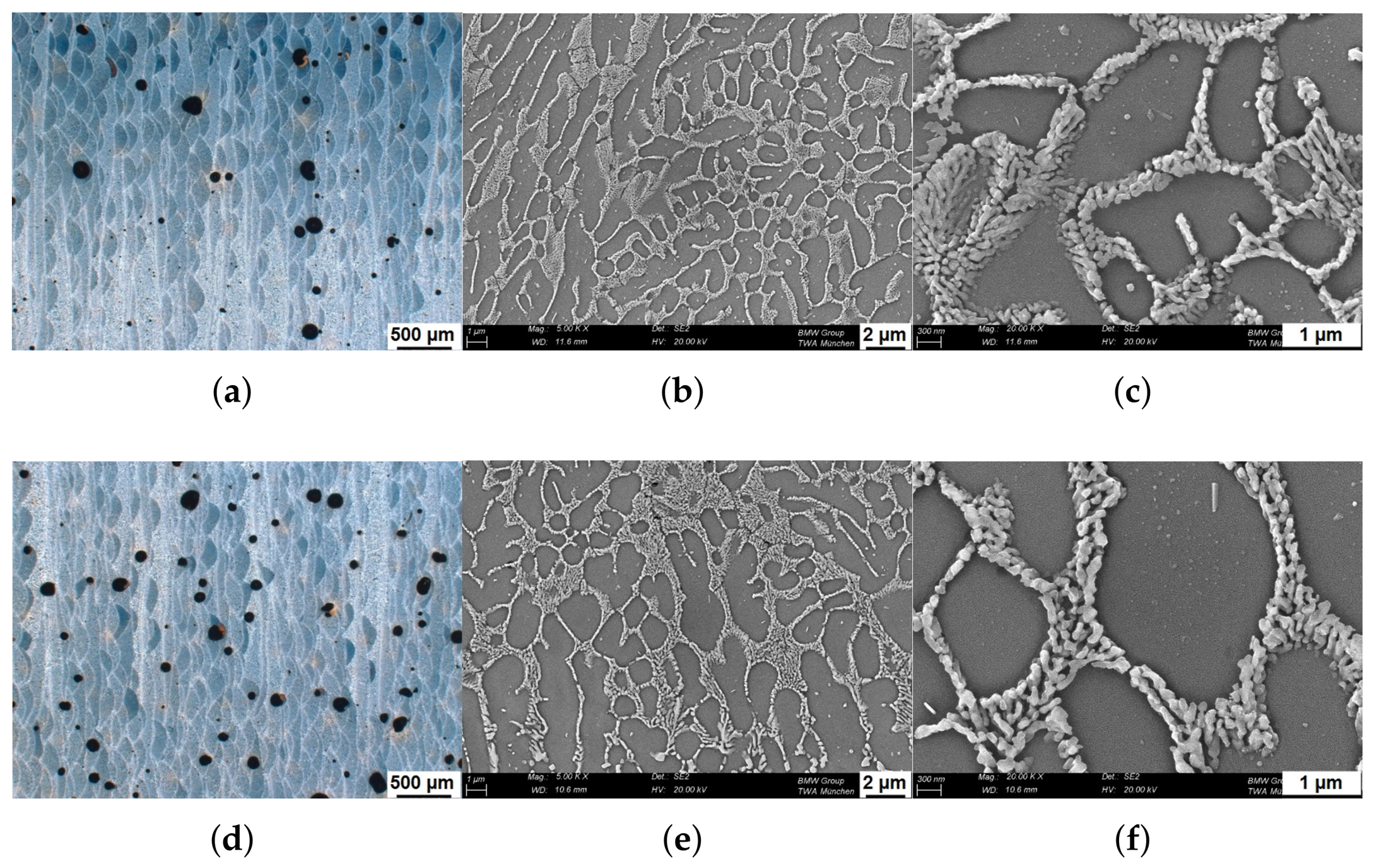
In the first use case, i.e., maximizing YS and UTS, both parameter sets revealed a comparable macroscopic structure in the light-optical microscopy images (Figure 6). Both samples exhibited similar weld bead characteristics, where the WM samples had slightly deeper weld pools. In both samples, irregular-shaped lack-of-fusion porosity was visible, yet the level for the WM samples was significantly higher with 2.34% than the single model samples with 0.49% porosity.
Figure 6.
Microstructure images for use case 1—strength optimization; microstructure for WM model (a–c) and single models (d–f); light microscopy at 25× magnification (a,d); SEM images at 5000× (b,e); and 20,000× magnification (c,f).
The SEM images at 5000× magnification revealed that the WM samples had a characteristic cellular structure of Al-Si eutectic surrounded by the -Al matrix, which was not as apparent for the samples of a single model parameter. Its eutectic appeared ragged and disrupted. At 20,000× magnification, the WM specimen showed very fine Si precipitates in the -Al matrix, which might be due to the high cooling rates characteristic for PBF-LB [48]. This phenomenon was much more pronounced in the single model samples.
As it is reported in the literature, the size of this cellular structure has a profound influence on the mechanical properties of AlSi10Mg0.5 in its as-build state. The finer the structure, the higher the tensile strength becomes due to hindered dislocation movement. The fine Si precipitates enhanced this effect even further [49,50,51]. The elevated lack-of-fusion porosity levels counteracted this effect, which might explain the lower validation values compared with its predictions. Especially the single model parameter set was affected by its high amount of pores.
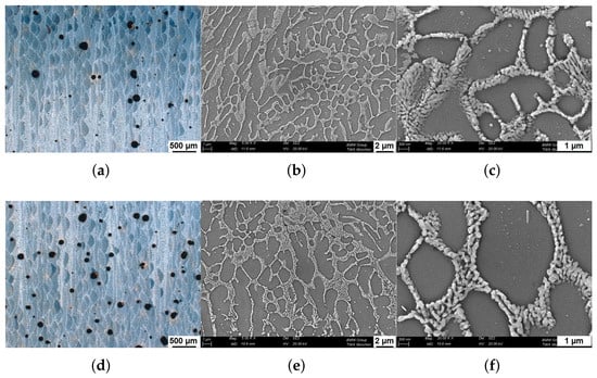
In the second use case to maximize elongation, again both parameter sets looked similar to each other in the macroscopic structure (Figure 7). The light-optical microscopy images showed characteristic round key-hole porosity, however, with different amounts of pores in one sample. The WM specimen had 1.45%, and the single model parameter set produced 3.14% porosity. Both levels affected the elongation at break due to the quantity of pores; however, the single model parameter set had roughly twice the porosity level. This may present a reason why the samples fall short on its prediction, despite the fact that porosity is implicitly part of the models, due to their inherent porosity in the training samples.
Figure 7.
Microstructure images for use case 2—ductility optimization; microstructure for WM model (a–c) and single models (d–f); light microscopy at 25× magnification (a,d); SEM images at 5000× (b,e); and 20,000× magnification (c,f).
Since both parameter sets had rather high heat input and low velocities, the material absorbed comparatively high amounts of energy; thus, it can be assumed that cooling rates were reduced during the rather slow process. These processing conditions lead to pronounced evaporation of metal in the laser spot, and key hole porosity was prevalent as reported by Patel et al. [40]. The microstructure in the SEM images appeared as a well-formed Al-Si network. It seemed a little coarser both in the cellular structure and within the AlSi-eutectic compared with the samples of the first use case. Additionally, the precipitates within the -Al matrix were much less apparent, which also supports the above-mentioned notion of overheating, leading to more time for segregation during solidification. The coarser sub-cell structure and the lack of Si precipitates imply that lower strength values are to be expected, which the actual values matched. Additionally, higher heat input and thus less pronounced temperature gradients reduced the amount of residual stresses within the material as reported by Ali et al. [52]. This combined with the rather high porosity presumably leads to a softer and comparatively annealed state of the material and thus provides some explanation of the low mechanical properties measured.
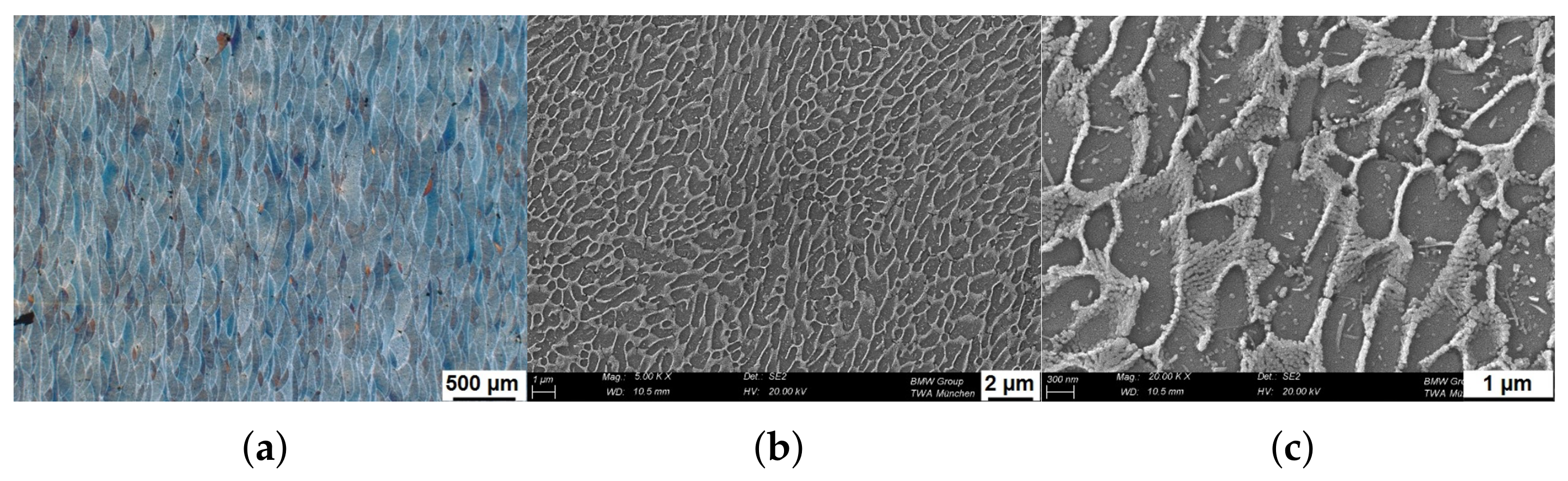
In the third use case to maximize productivity, the parameter set showed very reduced porosity of 0.21% and a uniform layered structure with shallow weld beads in the light-optical microscopy image in Figure 8. The cellular structure in the SEM images also appeared to be rather uniform, yet much finer than compared with the samples of the first two use cases. The fine cellular structure and the rather pronounced amount of precipitations in the -Al matrix may reflected the high printing speed and imply elevated tensile values based on the aforementioned literature. As stated before, the mechanical properties of this parameter set were comparable with the results for use cases 1. The low porosity and the fine microstructure of the productivity use case seemed to be beneficial for yielding high mechanical properties.
Figure 8.
Microstructure images for use case 3—productivity optimization; microstructure for single models (a–c); light microscopy at 25× magnification (a); SEM images at 5000× (b); and 20,000× magnification (c).
4. Conclusions and Outlook for Further Research
In the presented research, transfer learning was explored to translate pre-trained, neural network-based process models between non-identical PBF-LB machines. A small training dataset of 25 data vectors was used to further train existing NN models and adapt them to the new machine. It was tested to use the small dataset and minimize the empirical effort, i.e., time and resources, to yield exploitable models for optimizing tensile properties of the printed material.
The results showed that, with this minimal amount of training data, the transfer learning results showed mostly good fits for the target training data on the Trumpf machine. The test scores for YS reached up to = 75.5%, for UTS a maximum of = 82.1%, and for elongation, even = 92.0% was obtained. One exception to this was the NM model for elongation at break, which yielded completely unusable results with = −1897%.
Since it was possible to distinguish eight approaches based on the degrees of training freedom regarding the amount of trainable layers, every possible approach was compared for each target value. Based on the presented results, it did not become obvious, which degree of freedom the TL models were awarded, worked best in a global manner. Thus, a weighted mean model, which incorporated all eight models weighted by their -value, was derived.
The three validation scenarios revealed that both single models and the WM model yielded mostly usable predictions to optimize the mechanical properties and processing conditions. The WM model delivered more conservative estimates, which matched more with the actual data compared with the single model variants. The microstructure revealed that varying levels of porosity were present within the samples, which explained the deviations between prediction and validation values. Additionally, pore forms indicated tendencies to conduction-mode melting in the strength optimization use case and keyhole-mode melting in the maximizing ductility trials. These process conditions were also visible in the nanostructure in the SEM images. Low dl. heat input or high dl. velocities showed a much finer cellular structure (use cases 1 and 3) as compared with the coarser structures present in the ductility optimization use case with high dl. heat input and low dl. velocity.
The overall findings of this research were as follows:
- It is possible to use transfer learning to adapt existing processing models between PBF-LB machines.
- The amount of necessary training data and the resulting testing expenses can be kept rather low; one build job with 25 parameter variations was enough to adapt the TL models on the target system with comparable accuracy as the source model.
- The validation trials showed usable predictions in three real-world scenarios—optimization of (1) tensile strength, (2) ductility, and (3) productivity.
- Microstructure analysis revealed the process conditions expected from the melt mode diagram.
In an industrial context, these results show promising advances to enable more rapid qualification of new production machines based on the TL approach. The machine-specific process models can be used to determine usable production parameters fast, which can then be refined. Thus, the qualification effort can be focused more on actual productive parameters, rather than the basic exploration of the process parameter space.
Besides these findings, the limitations of this study based on the small amounts of data are given for upcoming research. First, it became apparent that, due to the limited data size, significant fold-to-fold variations in the test scores and even negative fits occurred. This showed that the models were highly sensitive to sample quality and outliers due to the available data quantity per subsample. For further research, it might be recommended to use leave-one-out cross-validation for model evaluation. Moreover, when optimized parameters are to be used productively, a second verification lap to statistically safeguard the chosen parameter across multiple build jobs is still considered necessary.
Second, building the WM model with the averaged scores instead of the best folds to strengthen its reliability further is a topic to be explored in the future. In this case, models with negative average testing scores, e.g., the NM for elongation at break, must be excluded, and models showing negative -values in single folds could be excluded. Additionally, it can be tested if or how model exclusion limits strengthen the WM model. Moreover, developing quantitative metrics as selection criteria for the single models would strengthen the model’s exploitation for process optimization. This would also enable the automatic model evaluation and selection in future developments.
Third, the microstructure evaluation helped explain the findings for all three use cases. The training samples produced were not free of porosity; thus, the models’ predictions should include a certain porosity bias. However, the influence of porosity was not explicitly incorporated in the predictions. It became apparent that the porosity can vary significantly between processing conditions and the levels affected the mechanical properties. Thus, in future investigations, it appears to be beneficial to also model porosity to refine the predictions of the mechanical properties. Additionally, residual stresses and surface roughness could also influence the results and could further refine the resulting process models.
Author Contributions
F.F. was involved in project administration, conceptualization, methodology, formal analysis, validation, writing of the original manuscript, review and editing, visualization, and investigation. S.B. worked on data curation and formal analysis, conceptualization and writing of the original manuscript. M.K. contributed to resources, data curation, validation, and writing of the original draft. P.M. helped with supervision and editing. All authors have read and agreed to the published version of the manuscript.
Funding
This work was partially funded by Technology Transfer Program Lightweight Construction (Technologietransfer-Programm Leichtbau—TTP LB) by the Federal Ministry for Economic Affairs and Climate Action, Germany (Grant 03LB2009C).
Institutional Review Board Statement
Not applicable.
Informed Consent Statement
Not applicable.
Data Availability Statement
The datasets generated and analyzed during the current study are available in the Zenodo repository via https://doi.org/10.5281/zenodo.19075965 (accessed on 17 March 2026).
Conflicts of Interest
The following authors are an employee of the company: BMW AG, Knorrstr. 147, 80788 Munich: Florian Funcke, Sebastian Brummer and Marinus Kolbinger. Peter Mayr declares no conflicts of interests.
Appendix A. Hyperparameters for TL Models
Table A1.
Hyperparameters for YS models.
Table A2.
Hyperparameters for UTS models.
Table A3.
Hyperparameters for A models.
Appendix B. Predicted Response Surfaces for Validation Use Cases
Figure A1.
Predicted response surface for ultimate tensile strength by WM model; parameter points for use case 1 (maximizing yield and tensile strength), use case 2 (maximizing ductility), and use case 3 (maximizing productivity) are given.
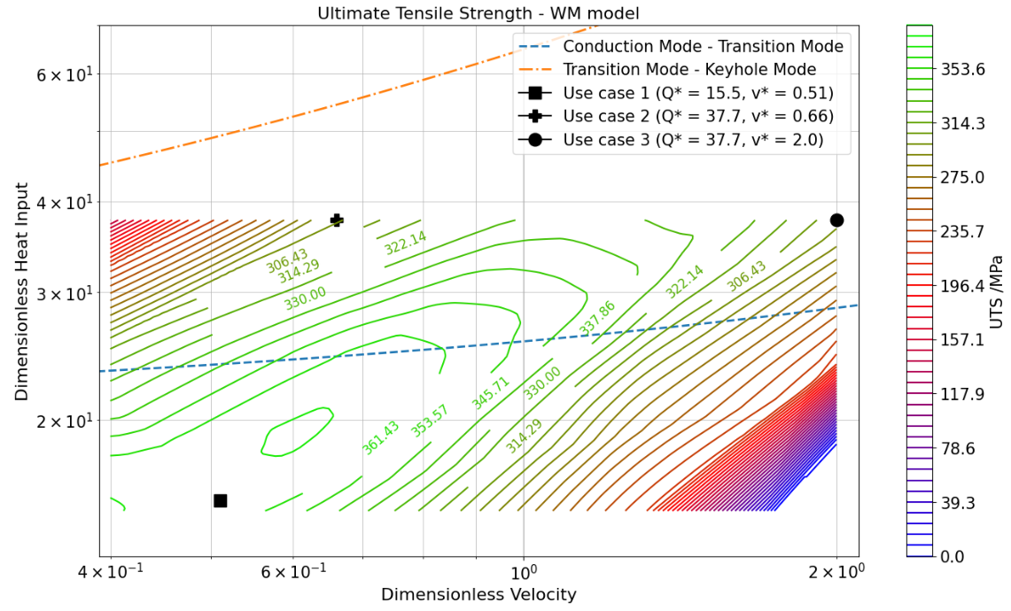
Figure A2.
Predicted response surface for elongation by WM model; parameter points for use case 1 (maximizing yield and tensile strength), use case 2 (maximizing ductility), and use case 3 (maximizing productivity) are given.
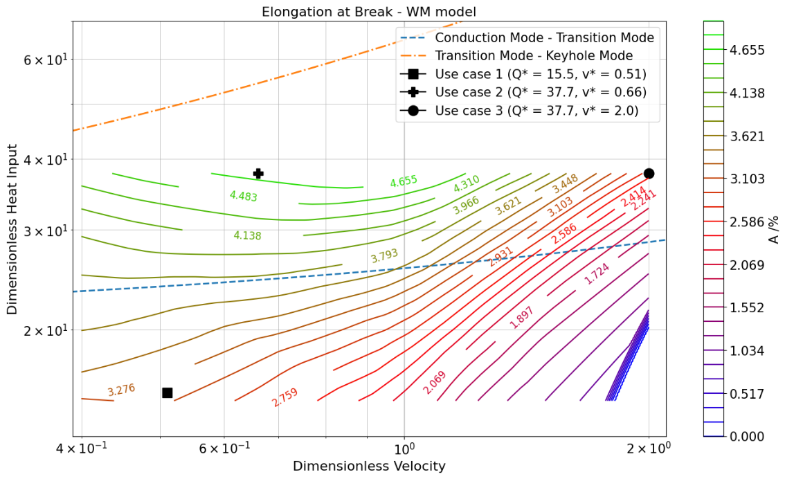
Figure A3.
Predicted response surface for yield strength by SLF model; parameter points for use case 1 (maximizing yield and tensile strength) and use case 2 (maximizing ductility) are given.
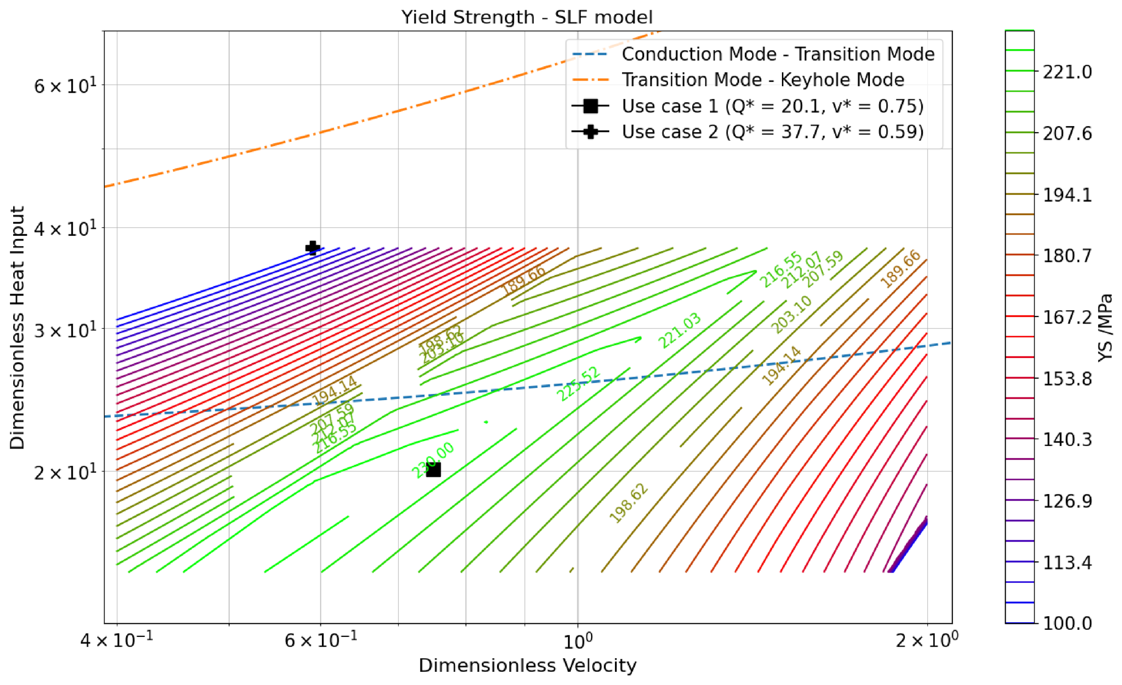
Figure A4.
Predicted response surface for ultimate tensile strength by FLT model; parameter points for use case 1 (maximizing yield and tensile strength) and use case 2 (maximizing ductility) are given.
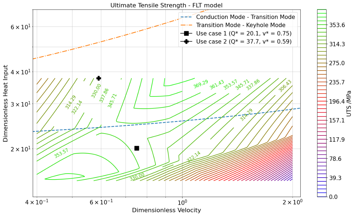
Figure A5.
Predicted response surface for elongation by FMT model; parameter points for use case 1 (maximizing yield and tensile strength) and use case 2 (maximizing ductility) are given.
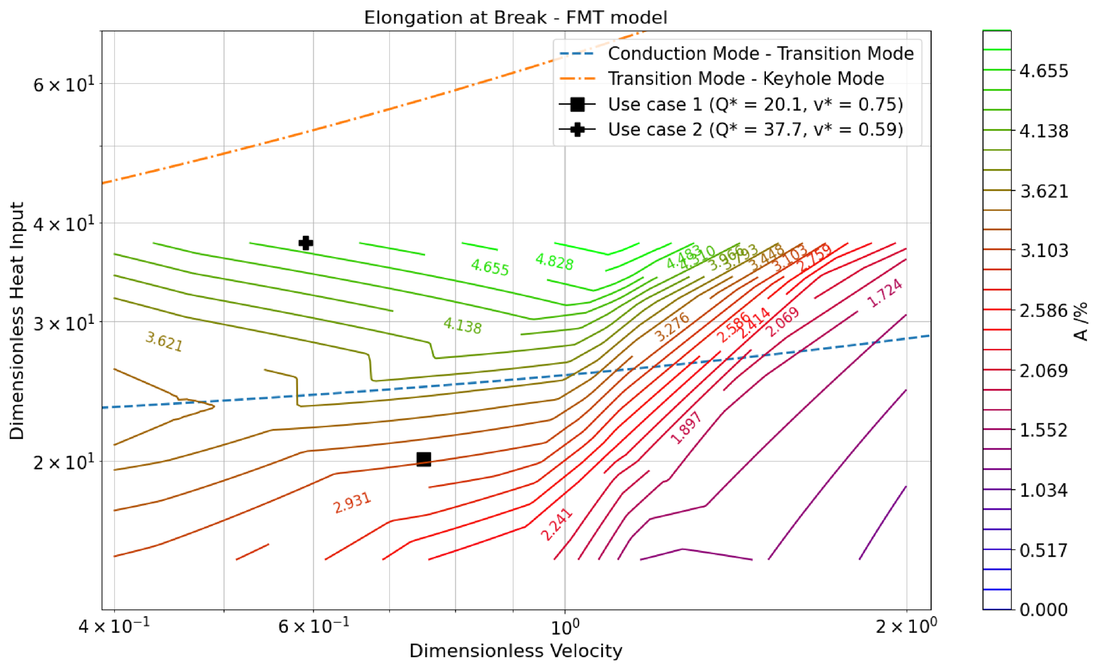
Figure A6.
Predicted response surface for yield strength by FMT model; parameter point for use case 3 (maximizing productivity) is given.
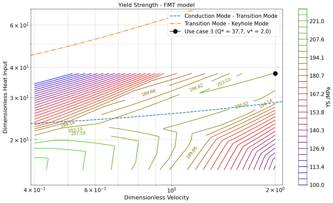
Figure A7.
Predicted response surface for ultimate tensile strength by SLT model; parameter point for use case 3 (maximizing productivity) is given.
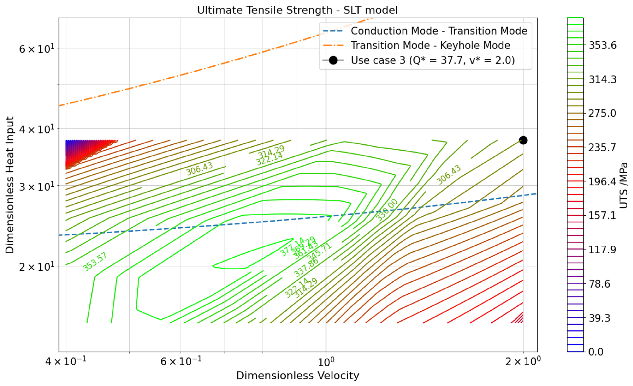
Figure A8.
Predicted response surface for elongation by FLT model; parameter point for use case 3 (maximizing productivity) is given.
References
- Bremen, S.; Meiners, W.; Diatlov, A. Selective Laser Melting: A manufacturing technology for the future? Laser Tech. J. 2012, 9, 33–38. [Google Scholar] [CrossRef] [Scilit]
- Riener, K.; Pfalz, T.; Funcke, F.; Leichtfried, G. Processability of high-strength aluminum 6182 series alloy via laser powder bed fusion (LPBF). Int. J. Adv. Manuf. Technol. 2022, 119, 4963–4977. [Google Scholar] [CrossRef] [Scilit]
- Santos Macías, J.G.; Douillard, T.; Zhao, L.; Maire, E.; Pyka, G.; Simar, A. Influence on microstructure, strength and ductility of build platform temperature during laser powder bed fusion of AlSi10Mg. Acta Mater. 2020, 201, 231–243. [Google Scholar] [CrossRef] [Scilit]
- Trevisan, F.; Calignano, F.; Lorusso, M.; Pakkanen, J.; Aversa, A.; Ambrosio, E.; Lombardi, M.; Fino, P.; Manfredi, D. On the Selective Laser Melting (SLM) of the AlSi10Mg Alloy: Process, Microstructure, and Mechanical Properties. Materials 2017, 10, 76. [Google Scholar] [CrossRef] [Scilit]
- Paradise, P.; Patil, D.; Van Handel, N.; Temes, S.; Saxena, A.; Bruce, D.; Suder, A.; Clonts, S.; Shinde, M.; Noe, C.; et al. Improving Productivity in the Laser Powder Bed Fusion of Inconel 718 by Increasing Layer Thickness: Effects on Mechanical Behavior. J. Mater. Eng. Perform. 2022, 31, 6205–6220. [Google Scholar] [CrossRef] [Scilit]
- Gullane, A.; Murray, J.W.; Hyde, C.J.; Sankare, S.; Evirgen, A.; Clare, A.T. On the use of multiple layer thicknesses within laser powder bed fusion and the effect on mechanical properties. Mater. Des. 2021, 212, 110256. [Google Scholar] [CrossRef] [Scilit]
- Wang, J.; Jeong, S.G.; Kim, E.S.; Kim, H.S.; Lee, B.J. Material-agnostic machine learning approach enables high relative density in powder bed fusion products. Nat. Commun. 2023, 14, 6557. [Google Scholar] [CrossRef] [Scilit]
- Wen, H.; Huang, C.; Guo, S. The application of convolutional neural networks (CNNs) to recognize defects in 3D-printed parts. Materials 2021, 14, 2575. [Google Scholar] [CrossRef] [Scilit]
- Klein, J.; Jaretzki, M.; Schwarzenberger, M.; Ihlenfeldt, S.; Drossel, W.G. Automated porosity assessment of parts produced by Laser Powder Bed Fusion using Convolutional Neural Networks. Procedia CIRP 2021, 104, 1434–1439. [Google Scholar] [CrossRef] [Scilit]
- Liu, Q.; Wu, H.; Paul, M.J.; He, P.; Peng, Z.; Gludovatz, B.; Kruzic, J.J.; Wang, C.H.; Li, X. Machine-learning assisted laser powder bed fusion process optimization for AlSi10Mg: New microstructure description indices and fracture mechanisms. Acta Mater. 2020, 201, 316–328. [Google Scholar] [CrossRef] [Scilit]
- Nudelis, N.; Mayr, P. A Novel Classification Method for Pores in Laser Powder Bed Fusion. Metals 2021, 11, 1912. [Google Scholar] [CrossRef] [Scilit]
- Gu, Z.; Sharma, S.; Riley, D.A.; Pantawane, M.V.; Joshi, S.S.; Fu, S.; Dahotre, N.B. A universal predictor-based machine learning model for optimal process maps in laser powder bed fusion process. J. Intell. Manuf. 2022, 34, 3341–3363. [Google Scholar] [CrossRef] [Scilit]
- Chang, T.W.; Liao, K.W.; Lin, C.C.; Tsai, M.C.; Cheng, C.W. Predicting magnetic characteristics of additive manufactured soft magnetic composites by machine learning. Int. J. Adv. Manuf. Technol. 2021, 114, 3177–3184. [Google Scholar] [CrossRef] [Scilit]
- Song, B.U.; Choi, J.P.; Lee, P.H.; Jung, M.K.; Shin, D.; Ha, T.; Lee, I. Efficient Optimization of Magnetic Properties of Fe–4.5Si Alloy in Laser Powder Bed Fusion (LPBF). Int. J. Precis. Eng. Manuf.-Green Technol. 2025. [Google Scholar] [CrossRef] [Scilit]
- Muscat, R.; Mahfouf, M. Predicting Charpy Impact Energy for Heat-Treated Steel using a Quantum-Membership-Function-based Fuzzy Model. IFAC-PapersOnLine 2016, 49, 138–142. [Google Scholar] [CrossRef] [Scilit]
- Smyrnov, M.; Funcke, F.; Kabliman, E. Prediction of material toughness using ensemble learning and data augmentation. Philos. Mag. Lett. 2024, 104, 2372497. [Google Scholar] [CrossRef] [Scilit]
- Wu, S.-w.; Yang, J.; Cao, G.-m. Prediction of the Charpy V-notch impact energy of low carbon steel using a shallow neural network and deep learning. Int. J. Miner. Metall. Mater. 2021, 28, 1309–1320. [Google Scholar] [CrossRef] [Scilit]
- Scime, L.; Joslin, C.; Collins, D.A.; Sprayberry, M.; Singh, A.; Halsey, W.; Duncan, R.; Snow, Z.; Dehoff, R.; Paquit, V. A Data-Driven Framework for Direct Local Tensile Property Prediction of Laser Powder Bed Fusion Parts. Materials 2023, 16, 7293. [Google Scholar] [CrossRef] [Scilit]
- Dejene, N.D.; Lemu, H.G. Characterisation and prediction of mechanical properties in laser powder bed fusion-printed parts: A comparative analysis using machine learning. Mater. Technol. 2024, 39, 2419228. [Google Scholar] [CrossRef] [Scilit]
- Moshiri, M.; Candeo, S.; Carmignato, S.; Mohanty, S.; Tosello, G. Benchmarking of Laser Powder Bed Fusion Machines. J. Manuf. Mater. Process. 2019, 3, 85. [Google Scholar] [CrossRef] [Scilit]
- Haeckel, F.; Meixlsperger, M.; Burkert, T. Technological Challenges for Automotive Series Production in Laser Beam Melting. In Proceedings of the 2017 International Solid Freeform Fabrication Symposium, Austin, TX, USA, 7–9 August 2017. [Google Scholar] [CrossRef]
- Reijonen, J.; Björkstrand, R.; Riipinen, T.; Que, Z.; Metsä-Kortelainen, S.; Salmi, M. Cross-testing laser powder bed fusion production machines and powders: Variability in mechanical properties of heat-treated 316L stainless steel. Mater. Des. 2021, 204, 109684. [Google Scholar] [CrossRef] [Scilit]
- Brown, C.U.; Jacob, G.; Stoudt, M.; Moylan, S.; Slotwinski, J.; Donmez, A. Interlaboratory Study for Nickel Alloy 625 Made by Laser Powder Bed Fusion to Quantify Mechanical Property Variability. J. Mater. Eng. Perform. 2016, 25, 3390–3397. [Google Scholar] [CrossRef] [Scilit]
- Ladewig, A.; Schlick, G.; Fisser, M.; Schulze, V.; Glatzel, U. Influence of the shielding gas flow on the removal of process by-products in the selective laser melting process. Addit. Manuf. 2016, 10, 1–9. [Google Scholar] [CrossRef] [Scilit]
- Reijonen, J.; Revuelta, A.; Riipinen, T.; Ruusuvuori, K.; Puukko, P. On the effect of shielding gas flow on porosity and melt pool geometry in laser powder bed fusion additive manufacturing. Addit. Manuf. 2020, 32, 101030. [Google Scholar] [CrossRef] [Scilit]
- Anwar, A.B.; Pham, Q.C. Selective laser melting of AlSi10Mg: Effects of scan direction, part placement and inert gas flow velocity on tensile strength. J. Mater. Process. Technol. 2017, 240, 388–396. [Google Scholar] [CrossRef] [Scilit]
- Metelkova, J.; Kinds, Y.; Kempen, K.; de Formanoir, C.; Witvrouw, A.; Van Hooreweder, B. On the influence of laser defocusing in Selective Laser Melting of 316L. Addit. Manuf. 2018, 23, 161–169. [Google Scholar] [CrossRef] [Scilit]
- Mancisidor, A.; Garciandia, F.; Sebastian, M.S.; Álvarez, P.; Díaz, J.; Unanue, I. Reduction of the Residual Porosity in Parts Manufactured by Selective Laser Melting Using Skywriting and High Focus Offset Strategies. Phys. Procedia 2016, 83, 864–873. [Google Scholar] [CrossRef] [Scilit]
- TRUMPF Laser- und Systemtechnik GmbH. TruPrint 5000—Highly Productive 3D Printing for Industrial Serial Production; TRUMPF Laser- und Systemtechnik GmbH: Ditzingen, Germany, 2025. [Google Scholar]
- Nikon SLM Solutions AG. SLM 500; Nikon SLM Solutions AG: Lübeck, Germany, 2025. [Google Scholar]
- Pan, S.J.; Yang, Q. A Survey on Transfer Learning. IEEE Trans. Knowl. Data Eng. 2010, 22, 1345–1359. [Google Scholar] [CrossRef] [Scilit]
- Tang, Y.; Rahmani Dehaghani, M.; Wang, G.G. Review of transfer learning in modeling additive manufacturing processes. Addit. Manuf. 2023, 61, 103357. [Google Scholar] [CrossRef] [Scilit]
- Tang, Y.; Dehaghani, M.R.; Wang, G.G. Comparison of Transfer Learning based Additive Manufacturing Models via A Case Study. arXiv 2023, arXiv:2305.11181. [Google Scholar] [CrossRef] [Scilit]
- Tang, Y.; Rahmani Dehaghani, M.; Sajadi, P.; Wang, G.G. Selecting subsets of source data for transfer learning with applications in metal additive manufacturing. J. Intell. Manuf. 2024, 36, 3185–3206. [Google Scholar] [CrossRef] [Scilit]
- Liu, S.; Stebner, A.P.; Kappes, B.B.; Zhang, X. Machine learning for knowledge transfer across multiple metals additive manufacturing printers. Addit. Manuf. 2021, 39, 101877. [Google Scholar] [CrossRef] [Scilit]
- Bahari-Sambran, F.; Orozco-Caballero, A.; Carreño, F.; Cepeda-Jiménez, C. Predictive processing maps for laser-powder bed fusion using transfer learning and melt pool geometry. Adv. Ind. Manuf. Eng. 2025, 11, 100168. [Google Scholar] [CrossRef] [Scilit]
- Skiadopoulos, M.; Kifer, D.; Shokouhi, P. A transfer learning approach to the prediction of porosity in additively manufactured metallic components. NDT E Int. 2025, 157, 103531. [Google Scholar] [CrossRef] [Scilit]
- Luo, Q.; Huang, N.; Bartles, D.L.; Simpson, T.W.; Beese, A.M. Harnessing of in situ processing data to predict mechanical properties of laser powder bed fusion AlSi10Mg. J. Intell. Manuf. 2025, 37, 909–931. [Google Scholar] [CrossRef] [Scilit]
- Funcke, F.; Forster, T.; Kolbinger, M.; Prudlik, R.; Mayr, P. Grey Box Modelling to Predict Tensile Properties in PBF-LB. Res. Sq. 2025. [Google Scholar] [CrossRef] [Scilit]
- Patel, S.; Vlasea, M. Melting modes in laser powder bed fusion. Materialia 2020, 9, 100591. [Google Scholar] [CrossRef] [Scilit]
- Paszke, A.; Gross, S.; Massa, F.; Lerer, A.; Bradbury, J.; Chanan, G.; Killeen, T.; Lin, Z.; Gimelshein, N.; Antiga, L.; et al. Pytorch: An imperative style, high-performance deep learning library. In Proceedings of the Advances in Neural Information Processing Systems, Vancouver, BC, Canada, 8–14 December 2019; Volume 32. [Google Scholar]
- LeNail, A. NN-SVG: Publication-Ready Neural Network Architecture Schematics. J. Open Source Softw. 2019, 4, 747. [Google Scholar] [CrossRef] [Scilit]
- Soekhoe, D.; van der Putten, P.; Plaat, A. On the Impact of Data Set Size in Transfer Learning Using Deep Neural Networks. In Advances in Intelligent Data Analysis XV; Springer International Publishing: Berlin/Heidelberg, Germany, 2016; pp. 50–60. [Google Scholar] [CrossRef] [Scilit]
- Murphy, K.P. Probabilistic Machine Learning: An Introduction; MIT Press: Cambridge, MA, USA, 2022. [Google Scholar]
- Raschka, S. Machine Learning Q an AI; No Starch Press: San Francisco, CA, USA, 2024. [Google Scholar]
- Johnson, N.; Vulimiri, P.; To, A.; Zhang, X.; Brice, C.; Kappes, B.; Stebner, A. Invited review: Machine learning for materials developments in metals additive manufacturing. Addit. Manuf. 2020, 36, 101641. [Google Scholar] [CrossRef] [Scilit]
- Rahaman, M.; Mu, W.; Odqvist, J.; Hedström, P. Machine Learning to Predict the Martensite Start Temperature in Steels. Metall. Mater. Trans. A 2019, 50, 2081–2091. [Google Scholar] [CrossRef] [Scilit]
- Van Cauwenbergh, P.; Samaee, V.; Thijs, L.; Nejezchlebová, J.; Sedlák, P.; Iveković, A.; Schryvers, D.; Van Hooreweder, B.; Vanmeensel, K. Unravelling the multi-scale structure–property relationship of laser powder bed fusion processed and heat-treated AlSi10Mg. Sci. Rep. 2021, 11, 6423. [Google Scholar] [CrossRef] [Scilit] [PubMed]
- Kan, W.H.; Nadot, Y.; Foley, M.; Ridosz, L.; Proust, G.; Cairney, J.M. Factors that affect the properties of additively-manufactured AlSi10Mg: Porosity versus microstructure. Addit. Manuf. 2019, 29, 100805. [Google Scholar] [CrossRef] [Scilit]
- Kempf, A.; Hilgenberg, K. Influence of sub-cell structure on the mechanical properties of AlSi10Mg manufactured by laser powder bed fusion. Mater. Sci. Eng. A 2020, 776, 138976. [Google Scholar] [CrossRef] [Scilit]
- Yang, T.; Liu, T.; Liao, W.; MacDonald, E.; Wei, H.; Zhang, C.; Chen, X.; Zhang, K. Laser powder bed fusion of AlSi10Mg: Influence of energy intensities on spatter and porosity evolution, microstructure and mechanical properties. J. Alloys Compd. 2020, 849, 156300. [Google Scholar] [CrossRef] [Scilit]
- Ali, H.; Ghadbeigi, H.; Mumtaz, K. Residual stress development in selective laser-melted Ti6Al4V: A parametric thermal modelling approach. Int. J. Adv. Manuf. Technol. 2018, 97, 2621–2633. [Google Scholar] [CrossRef] [Scilit]

Disclaimer/Publisher’s Note: The statements, opinions and data contained in all publications are solely those of the individual author(s) and contributor(s) and not of MDPI and/or the editor(s). MDPI and/or the editor(s) disclaim responsibility for any injury to people or property resulting from any ideas, methods, instructions or products referred to in the content. |
© 2026 by the authors. Licensee MDPI, Basel, Switzerland. This article is an open access article distributed under the terms and conditions of the Creative Commons Attribution (CC BY) license.