Evaluation of Time-Dependent Magnetic Losses of Permanent Magnets

Abstract

Time-dependent magnetization losses critically affect the performance of permanent magnets during their service lifetime. Quantifying these losses remains challenging, as existing analytical models and simulation tools lack suitable functions for accurate prediction. This work introduces a practical method to quantify these losses using the magnetic viscosity parameter and to predict future behavior via the time-dependent fluctuation field. Measurements on several magnet grades demonstrate that long-term stability can be reliably estimated with this approach, supporting both analytical evaluation and direct implementation in numerical simulations. Validation against long-term experiments confirms the accuracy of the method and its suitability for predicting magnetization evolution, enabling more targeted material selection.

1. Introduction

Permanent magnets are essential components in various systems, including sensors, linear and rotary actuators, electric motors, and generators [1,2,3]. A central challenge in these applications is ensuring long-term magnetization stability under varying operating conditions [4,5]. Key requirements for permanent magnet materials in technical applications are a high remanence, a sufficiently high coercive field strength, and long-term stability against field- and temperature-induced demagnetization. In other words, time-dependent magnetization changes must remain within acceptable limits over the intended service life.

Permanent magnets are metastable systems, which causes hysteresis and makes them susceptible to irreversible magnetization losses under external influences such as magnetic fields and elevated temperatures [4,6]. Thermal fluctuations additionally cause time-dependent magnetization losses, making time another critical factor [7,8,9]. There is a well-established theoretical framework describing these time-dependent magnetization changes, usually referred to as magnetic viscosity or the magnetic aftereffect [9,10]. A particularly useful concept for the estimation of future magnetization changes is the introduction of an effective magnetic fluctuation field [9]. Although initially described for single-domain materials, the method is also applicable to various permanent magnet materials, such as NdFeB, as demonstrated in previous works [10,11,12,13,14].

However, these approaches are predominantly theoretical. This work complements them by providing an application-oriented perspective by presenting results of different material grades of permanent magnets and demonstrating the use of the fluctuation field for the design of robust permanent magnet applications. Furthermore, a method is proposed to incorporate time dependency into numerical analyses, overcoming limitations of conventional finite element (FE) software that typically considers only peak magnetic fields and temperatures [15,16]. This approach enables more accurate magnetic system design by reducing overdesign in terms of coercive field strength through specific material selection, thereby minimizing the use of critical heavy rare earths [17] and associated costs.

2. Physical Background

Permanent magnets usually operate within the second quadrant of the hysteresis curve, where the magnetization is aligned opposite to the applied magnetic field. Favorable combinations of material properties such as exchange interaction and magnetocrystalline anisotropy result in energy barriers, which prevent magnetization reversal [6,18]. These energy barriers change with the applied field and with temperature: At any given temperature, increasing the demagnetizing field will reduce the height of the barriers until they eventually disappear, causing immediate magnetization reversal [9,18,19].

The immediate change in polarization $J$ is thus characterized by the change in polarization per change in the applied field $H$. This relation is quantified by the total differential magnetic susceptibility ${\chi }^{tot}$, defined as the sum of reversible and irreversible contributions, ${\chi }^{rev}$ and ${\chi }^{irr}$ [9,14]:

$${\chi }^{tot}={\chi }^{rev}+{\chi }^{irr}={\displaystyle \frac{{∆J}^{tot}}{{∆H}^{tot}}}$$

(1)

Based on this relation, Figure 1a illustrates a schematic $J\left(H\right)$-hysteresis curve, highlighting the regions of reversible and irreversible changes during the application of an external field. The hysteresis curves can be roughly sectioned into a linear region, a knee region, and a steep region.

•

The linear region is dominated by reversible changes (green marking): Starting from $H$ = 0 at remanence $J_r$, increasing the field to $H_A$ (point A) results in $J_A$. Reducing the field back to $H$ = 0 returns the initial polarization state $J_r$, showing that the decrease in polarization $∆J^{rev}$ to $J_A$ was fully reversible (quantified by reversible susceptibility ${\chi }^{rev}$).

•

The knee region (orange marking) is the area in the hysteresis curve where irreversible losses start to increase significantly, marking the transition between mainly reversible changes and irreversible demagnetization [20]. Beyond the knee point, for example, at field $H_B$ (point B), polarization $J_B$, originating from the initial remanent polarization $J_r$, consists of reversible and irreversible contributions and can be expressed as $J_B=J_r-\mathrm{\Delta }{J}^{rev}-\mathrm{\Delta }{J}^{irr}.$ Reducing the field back to $H=0$ follows a slope similar to the reversible region, leaving only the irreversible polarization contribution $\mathsf{\Delta }{J}^{\mathit{irr}}$ (quantified via the irreversible susceptibility ${\chi }^{\mathit{irr}}$).

•

The steep region, located between the knee point and the coercivity (red marking), is dominated by irreversible losses and represents the critical part of the hysteresis curve.

Figure 1. Schematic hysteresis curve illustrating relevant magnetic properties (exemplary curve with exaggerated shape). (a) Linear, knee, and steep regions indicate the transition from mainly reversible changes in the linear region to predominantly irreversible losses in the steep region. For example, a field change from $H$ = 0 to $H_A$ reduces the polarization from $J_r$ to $J_A$; reducing the field back to $H$ = 0 restores the initial remanent state $J_r$, confirming that the change in polarization $\Delta J^{rev}$ is reversible. In contrast, increasing the field from $H=0$ to $H_B$ at $J_B$ results in both reversible and irreversible changes $\mathrm{\Delta }{J}^{irr}.$ Reducing the field back to $H$ = 0 shows the irreversible decrease. (b) Visualization of the magnetic viscosity parameter and fluctuation field concepts. The magnetic viscosity parameter is determined from an initial field increase (e.g., from $H_A$ with $J_A$ to $H_B$ with $J_B$) for the determination of the differential susceptibility. During a constant field $H_B$, the time-dependent polarization decrease $\mathrm{\Delta }{J}^{\mathit{t.d.}}$ (pink) reduces the polarization from $J_B$ (point B) to $J_C$ (point C). The same polarization state $J_C$ can also be obtained by applying a fictitious fluctuation field $H_f$ to the maximum field $H_B$, resulting in an effective field $H_D$ with $J\left(H_D\right)=J_C$, adapted from Ref. [9]. (c) Shows the time-dependent polarization decrease on a logarithmic time scale, indicating an approximately linear trend, with slope $S$ corresponding to the magnetic viscosity. Here, $t_0$ describes the time at which the polarization values show a linear trend on a logarithmic time scale.

Figure 1. Schematic hysteresis curve illustrating relevant magnetic properties (exemplary curve with exaggerated shape). (a) Linear, knee, and steep regions indicate the transition from mainly reversible changes in the linear region to predominantly irreversible losses in the steep region. For example, a field change from $H$ = 0 to $H_A$ reduces the polarization from $J_r$ to $J_A$; reducing the field back to $H$ = 0 restores the initial remanent state $J_r$, confirming that the change in polarization $\Delta J^{rev}$ is reversible. In contrast, increasing the field from $H=0$ to $H_B$ at $J_B$ results in both reversible and irreversible changes $\mathrm{\Delta }{J}^{irr}.$ Reducing the field back to $H$ = 0 shows the irreversible decrease. (b) Visualization of the magnetic viscosity parameter and fluctuation field concepts. The magnetic viscosity parameter is determined from an initial field increase (e.g., from $H_A$ with $J_A$ to $H_B$ with $J_B$) for the determination of the differential susceptibility. During a constant field $H_B$, the time-dependent polarization decrease $\mathrm{\Delta }{J}^{\mathit{t.d.}}$ (pink) reduces the polarization from $J_B$ (point B) to $J_C$ (point C). The same polarization state $J_C$ can also be obtained by applying a fictitious fluctuation field $H_f$ to the maximum field $H_B$, resulting in an effective field $H_D$ with $J\left(H_D\right)=J_C$, adapted from Ref. [9]. (c) Shows the time-dependent polarization decrease on a logarithmic time scale, indicating an approximately linear trend, with slope $S$ corresponding to the magnetic viscosity. Here, $t_0$ describes the time at which the polarization values show a linear trend on a logarithmic time scale.

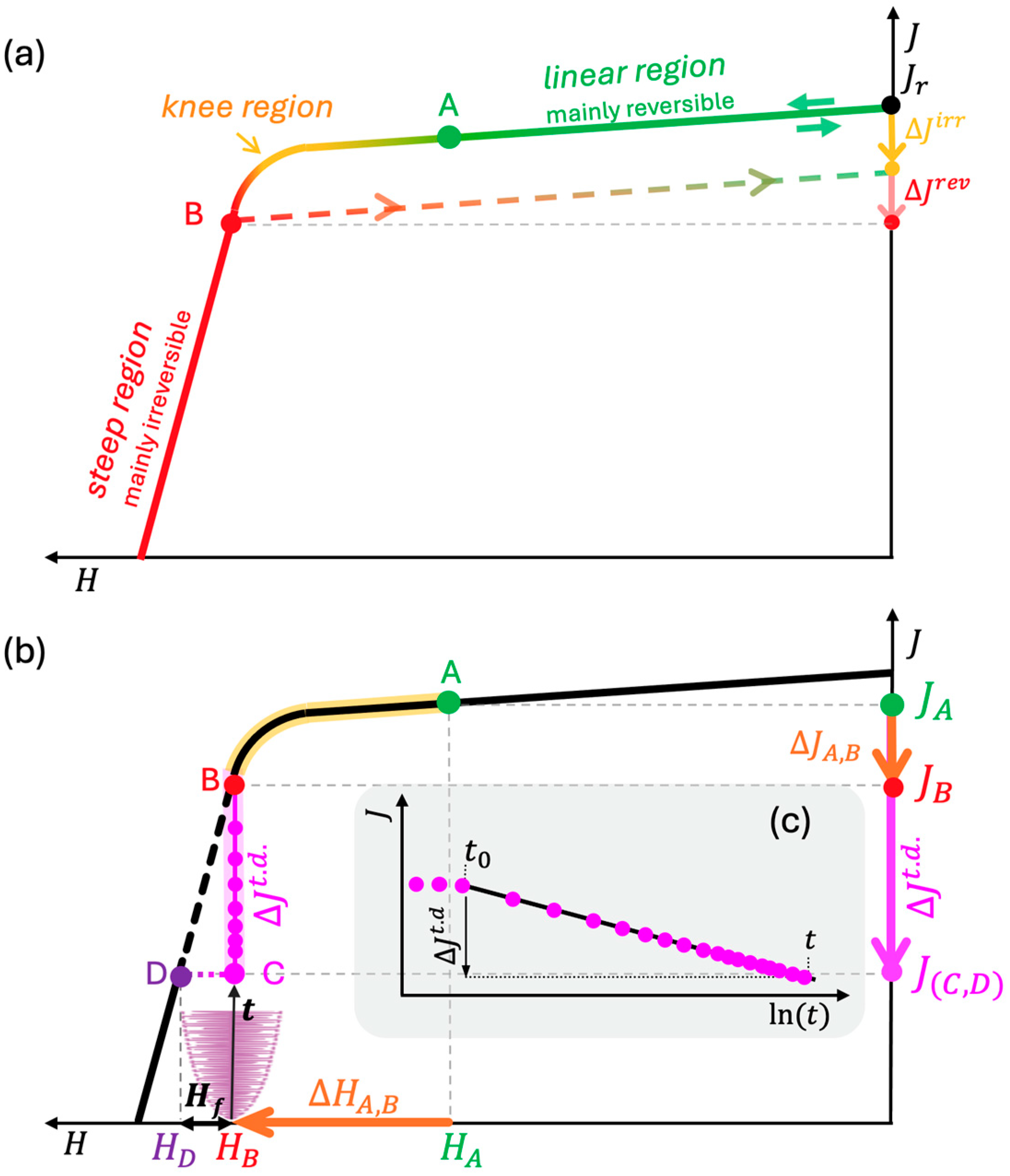
In addition to this immediate (direct) magnetization loss, some demagnetization is already observed at lower fields, evolving with time. This magnetization creep is known as magnetic viscosity or aftereffect, and is attributed to thermally activated transitions over energy barriers [8]. In practical terms, this combination of field and temperature defines a working point at which thermally activated fluctuations cause a time-dependent decrease in magnetization, e.g., from $J_B$ (point B) to $J_C$ (point C), given as $∆J^{\mathit{t.d.}}$ (see Figure 1b).

This decrease is irreversible over the exposure time $t$ relative to the reference time $t_0$, which denotes the time where the polarization shows an approximately linear trend on $\mathrm{l}\mathrm{n}\left(t\right)$, as visualized in Figure 1c.

The time-dependent magnetization decrease follows a logarithmic time law and is described by the magnetic viscosity $S$, defined as the ratio of polarization loss to the logarithm of time [7,8,9,10,14]:

$$∆J^{\mathit{t.d.}}=S\ast \mathrm{l}\mathrm{n}\left({\displaystyle \frac{t}{t_0}}\right),$$

(2)

The magnetic viscosity $S$ can serve as an indicator for the time-dependent demagnetization of permanent magnets. However, its application is challenging due to its strong dependence on external field $H$ and temperature $T$ [21,22]. Even minor changes in these conditions can lead to significant deviations, particularly in the steep region of the hysteresis curve.

A more useful approach arises from the observation that the time-dependent losses are roughly proportional to the direct field-induced losses, i.e., the magnetic viscosity $S$ is essentially proportional to the irreversible differential susceptibility ${\chi }^{irr}$ [7]. The ratio is therefore the magnetic viscosity parameter $S_v$ [9]:

$$S_v={\displaystyle \frac{S}{{\chi }^{irr}}}.$$

(3)

$S_v$ shows only moderate changes with the applied magnetic field and temperature [21]. For better illustration, $S_v$ can be determined by combining a field change, e.g., from $H_A$ (point A) to $H_B$ (point B) (light green in Figure 1b), to determine the differential susceptibility ${\chi }_{A,B}=∆J_{A,B}/∆H_{A,B}$, followed by a constant field $H_B,$ to measure the time-dependent polarization decrease $∆J^{\mathit{t.d.}}$ from $J_B$ (point B) to $J_C$ (point C) (light orange marking) as $S=∆J^{\mathit{t.d.}}/\ln \left(t/t_0\right)$.

The time-dependent decrease $∆J^{\mathit{t.d.}}$ in Figure 1b, from point B to C, yields the polarization state $J_C$ at $H_B$. According to Néel [9], the thermally activated losses leading to this polarization state can also be expressed by a fictitious fluctuation field $H_f$ as

$$H_f\left(t\right)=S_v \ast \ln \left({\displaystyle \frac{t}{t_0}}\right)$$

(4)

acting in addition to the actual magnetic field in the magnet. The sum of the applied magnetic field, e.g., $H_{max}=H_B$ and the fluctuation field $H_f\left(t\right)$ results in the field strength $H_D$, at $J_D$, corresponding to the same polarization state as $J_C$. Therefore, the resulting effective field as a function of time ($H_{eff}\left(t\right)$) is given by the sum of the applied magnetic field $H_{max}$ and $H_f\left(t\right)$:

$$H_{eff}\left(t\right)=H_{max}+H_f\left(t\right)$$

(5)

3. Experimental

To demonstrate the application of the magnetic viscosity parameter and the fluctuation field, commercially sintered NdFeB permanent magnets of grade N52 were investigated. All samples exhibit a remanence of $J_r$ = 1.4 T and differ in coercivity $H_{cj}$, with values of 1000 kA/m (standard), 1100 kA/m (M), 1350 kA/m (H), and 1600 kA/m (SH) at 25 °C. These magnet grades represent commonly used materials spanning a wide range of coercivities. All samples have dimensions of 20 × 10 × 5 mm³.

$J\left(H\right)$ curves were measured using a hysteresisgraph (Permagraph L, Magnet-Physik, Cologne, Germany). Measurements of the magnetic viscosity parameter $S_v$ were performed using a dedicated, non-destructive measurement approach that enables characterization of the full sample size, avoiding the need for specially cut samples as in conventional vibrating sample magnetometer (VSM) systems. The setup consists of an electromagnet with Hall probes and is described in detail in Ref. [21]. Finite-element simulations were carried out using Simcenter Magnet 2023 [15].

For validation, long-term comparison measurements were conducted using an open-circuit Helmholtz coil setup with a rotating sample under controlled temperature conditions, as described in Ref. [23].

4. Results and Discussion

The estimation of future magnetization losses is based on measurements of the magnetic viscosity parameter $S_v$ within Section 4.1, from which the fluctuation field $H_f\left(t\right)$ is derived (Section 4.2). This field can be applied qualitatively by estimating future magnetization losses from the $J\left(H\right)$ curves (Section 4.2), or quantitatively by incorporating it into finite element simulations for proper magnetic system design (Section 4.3).

4.1. Measurement Results of the Magnetic Viscosity Parameter $S_v$

$S_v$ measurements were conducted using a dedicated setup based on an electromagnetic yoke with Hall-probe sensors, as described in detail in previous work in Ref. [21]. This setup was chosen because it allows the determination of full sample sizes without destructive preparation, as required for VSM measurements. Commercially sintered permanent magnets of commonly used grade N52, with a remanent polarization of $J_r=$ 1.4 T, differing coercivities $H_{cj}$ of 1000 kA/m (standard), 1100 kA/m (M), 1350 kA/m (H), and 1600 kA/m (SH) at 25 °C, and dimensions of 20 × 10 × 5 mm³, were chosen. The total exposure time $t$ used in these measurements was approximately 180 s. Table 1 lists the measured $S_v$ values at the application-relevant field strength $H_{D5}$, defined as the field at which 5% irreversible demagnetization occurs [24]. These values were directly derived from the Hall probe measurements obtained with the dedicated measurement setup described above. Based on 10 measurements under identical conditions, a standard deviation of approximately 0.5 kA/m was determined for $S_v$ at the relevant $H_{D5}$ field strength.

Table 1. Measurement results of $S_v\left(H_{D5}\right)$ for different sample grades and temperatures. The measurements were conducted adapted from Ref. [21]. Additionally, the coercivity values $H_{cj}$ at each temperature are listed.

Sample	$\mathbf{RT}(~$25 °C)		70		100		130
	${\mathit{S}}_{\mathit{v}}$$({\mathit{H}}_{\mathit{D}5}$) [kA/m]	${\mathit{H}}_{\mathit{c}\mathit{j}}$ [kA/m]	${\mathit{S}}_{\mathit{v}}$$({\mathit{H}}_{\mathit{D}5}$) [kA/m]	${\mathit{H}}_{\mathit{c}\mathit{j}}$ [kA/m]	${\mathit{S}}_{\mathit{v}}$$({\mathit{H}}_{\mathit{D}5}$) [kA/m]	${\mathit{H}}_{\mathit{c}\mathit{j}}$ [kA/m]	${\mathit{S}}_{\mathit{v}}$$({\mathit{H}}_{\mathit{D}5}$) [kA/m]	${\mathit{H}}_{\mathit{c}\mathit{j}}$ [kA/m]
N52	6.4	990	6.2	650	5.2	473	4.8	342
N52-M	6.5	1100	6.3	695	5.3	512	5	376
N52-H	7	1350	6.4	889	5.5	692	5.5	507
N52-SH	7.8	1600	7.7	1083	7.5	860	7.4	615

Colored cells indicate the magnet grades and correspond to the colors of the J(H) curves in Figure 2.

A comparison of $S_v$ with the coercivity $H_{cj}$ of the samples shows a clear trend: $S_v$ increases with increasing coercivity. For instance, a small coercivity difference of 100 kA/m between N52 and N52-M leads to similar $S_v$ values of 6.4 and 6.5 kA/m. In contrast, N52-H and N52-SH show higher $S_v$ values of 7.0 and 7.8 kA/m, respectively, corresponding to their significantly higher coercivities (1350 kA/m (H) and 1600 kA/m (SH)). Increasing temperature reduces both coercivity and the values of $S_v$. Consequently, $S_v$, a material parameter is primarily determined by coercivity, and provides a robust and widely applicable metric for characterizing magnetic behavior independently of geometry. These findings are consistent with previous studies [21,22], confirming that $S_v$ increases with $H_{cj}$, while higher temperatures lead to reduced values as $H_{cj}$ decreases with temperature.

4.2. Implementing Magnetic Viscosity in Application Design

The concept of a fluctuation field, in principle, allows a quantitative prediction of irreversible long-term magnetization losses. However, in most cases, designers of permanent magnet applications will not be interested in a quantitative determination of magnetization losses: the actual goal is making sure that no significant losses occur at all. As shown in Section 2, this implies that the magnetic field in the magnets remains in the linear region of the demagnetization curve, staying well below the knee region, even under the worst-case combination of maximum field and temperature. The key for avoiding losses under these aspects is thus the choice of a magnet material with sufficiently high coercivity. At this stage of material selection, the concept of a fluctuation field becomes relevant. Based on the presented methodology, a typical design workflow can be formulated to start with the selection of a magnet material with very high intrinsic coercivity, conveniently represented by an idealized straight line instead of a real demagnetization curve. This will ensure that the magnitude of the demagnetizing fields in the magnets can be clearly visualized, whereas a real material with insufficient coercivity would limit the fields to values near the coercive field as the magnetization drops when field values reach the steep region of the hysteresis curve.

At this step, comparing the worst-case demagnetizing field $H_{max}$ with the demagnetization curves allows including the risk of long-term demagnetization by assuming an additional field $H_f\left(t\right),$ as given by Equation (4). Based on this, the maximum application field $H_{max}$ can be extended by the fluctuation field according to Equation (5), as a function of exposure time $t$. The exposure time $t$ is the cumulative duration of all intervals during which $H$ and $T$ simultaneously reach their maximum values over the entire operational period. The initial design is then evaluated to identify the worst-case combination of maximum field and temperature, which defines the coercivity required for the material. If such a material is deemed undesirable or difficult to procure, the designer may, at this point, decide to reduce the fields through design adjustments.

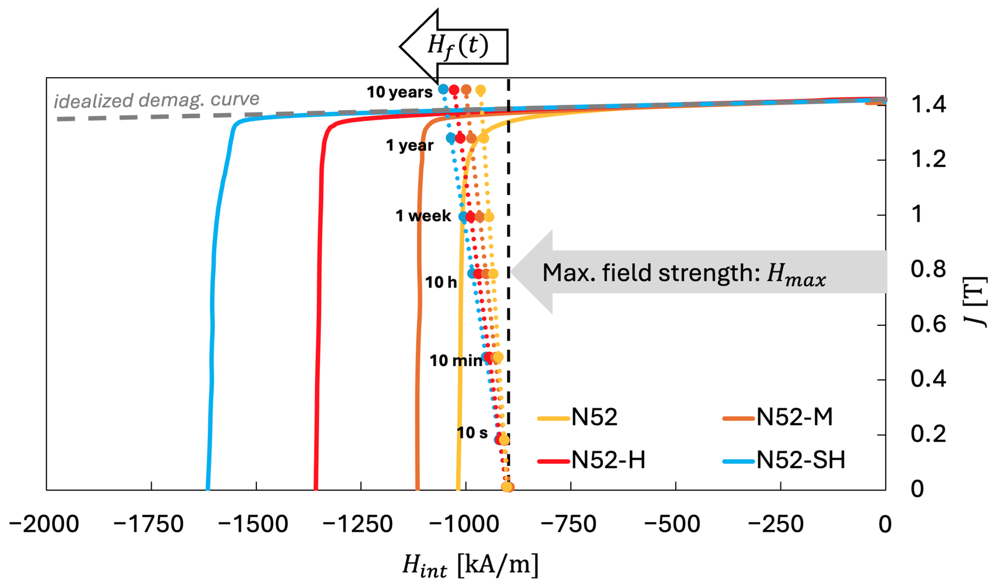
This approach is illustrated in Figure 2, which shows an idealized demagnetization curve (straight line) and the $J\left(H\right)$ material curves of the N52, N52-M, N52-H, and N52-SH samples from Table 1.

Figure 2. $J\left(H\right)$ curves of N52, N52-M, N52-H, and N52-SH sintered magnets at 25 °C (room temperature), along with an idealized demagnetization curve (gray dashed straight line). The worst-case demagnetizing field, $H_{max}$= −900 kA/m (exemplarily chosen), is shown together with the time-dependent fluctuation fields $H_f\left(t\right)$ for 10 s to 10 years. The color of each dashed $H_f\left(t\right)$ line indicates the corresponding $J\left(H\right)$ material curve, and the intersection of the line at a given exposure time $t$ with this curve represents the predicted magnetization state.

The corresponding fluctuation field $H_f\left(t\right)$ is shown over time frames ranging from 10 s to 10 years, based on a maximum applied magnetic field of $H_{max}$ = −900 kA/m at $T_{\mathrm{m}\mathrm{a}\mathrm{x}}$ = 25 °C. The intersection of each material’s $J\left(H\right)$ curve with the respective fluctuation field value (indicated as dashed lines in the corresponding color) represents the predicted magnetization state for the considered exposure time.

In this example, the applied magnetic field $H_{max}$ is already close to the knee region of the N52 sample. After 10 min, the estimated effective field reaches the critical knee region. Substantial demagnetization (by reaching the steeper part of the curve) is expected within 1 year. In contrast, the effective field of the N52-M sample remains in the stable linear region and approaches the knee region only after approximately 10 years. After 10 years under these maximum conditions, the estimated effective fields of the N52-H and N52-SH samples still lie within the linear (reversible) region, with N52-H already fulfilling long-term stability requirements.

The observed $S_v$ values range from about 4 to 8 kA/m, indicating that $S_v$ varies only within a narrow and predictable interval, enabling reliable use for magnetization prediction. Based on the $S_v$ data in Table 1, the maximum values were selected and listed in Table 2 as a guideline for additional fluctuation fields resulting from sample grade and time for the different sintered magnets. Notably, the $H_f$ values represent a rough estimation of the time dependency rather than exact values, as they depend on both the uncertainty of $S_v$ and the assumed reference time $t_0$.

Table 2. Fluctuation field values for commonly used magnet grades at different exposure times, based on the maximum measured $S_v$ values from Table 1, providing a guideline for direct application using N52 as reference grade.

$\mathbf{S}\mathbf{a}\mathbf{m}\mathbf{p}\mathbf{l}\mathbf{e} \mathbf{G}\mathbf{r}\mathbf{a}\mathbf{d}\mathbf{e}$	$\mathbf{Max}.{\mathit{S}}_{\mathit{v}}$ [kA/m]	${\mathit{H}}_{\mathit{f}}\left(\mathit{t}\right)[\mathbf{k}\mathbf{A}/\mathbf{m}]$
		$\mathit{t}$ = 1 Month	$\mathit{t}$ = 1 Year	$\mathit{t}$ = 10 Years
N52	6.5	96	112	127
N52-M
N52-H	7	103	121	137
N52-SH	8	118	138	157

Colored cells indicate the magnet grades and correspond to the colors of the J(H) curves in Figure 2.

4.3. Implementation of Time-Dependent Losses in Numerical Modeling Tools

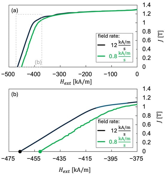
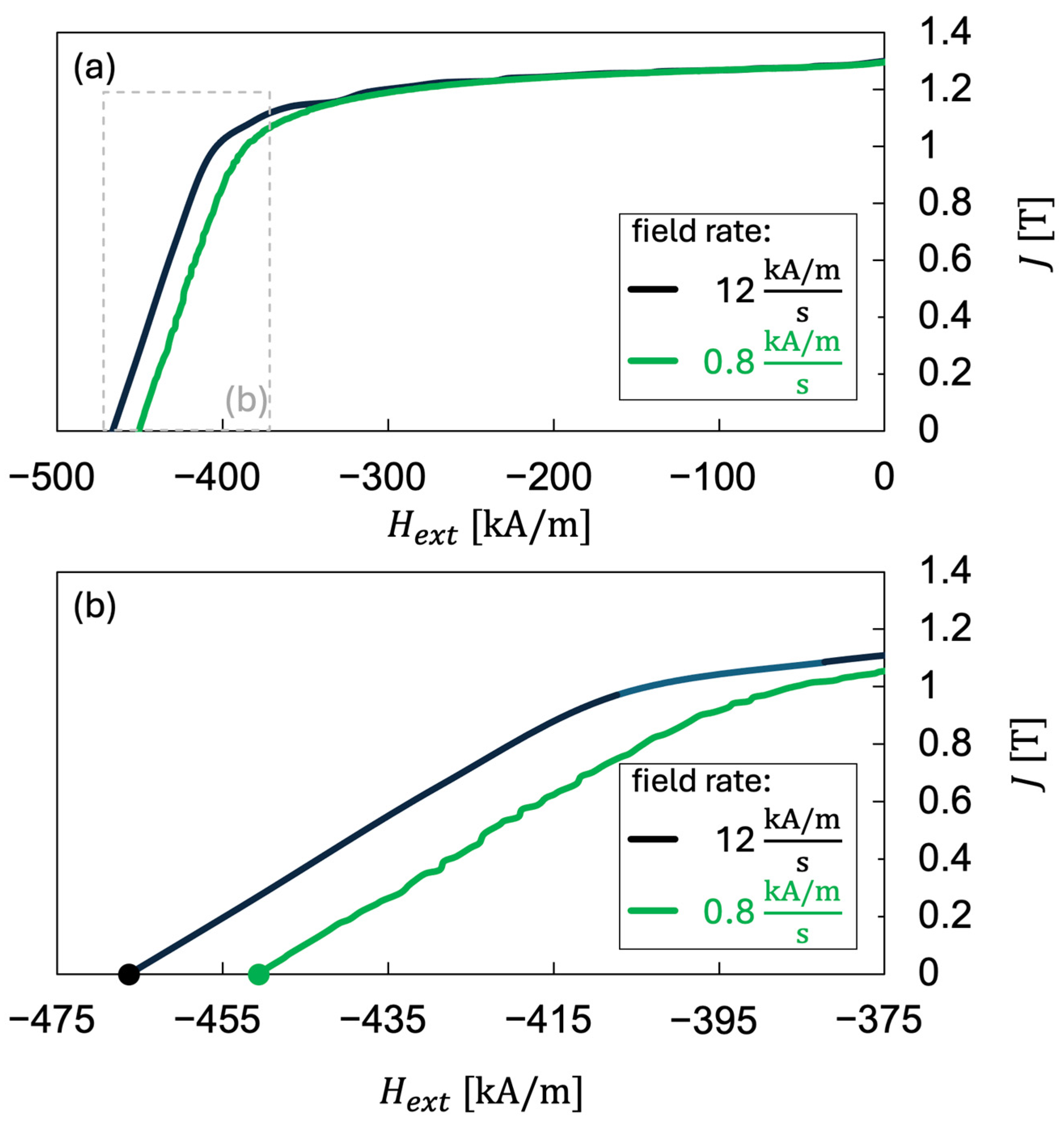
Common numerical software tools for magnetic system design, typically based on finite element (FE) methods, rely on static, single-valued $B\left(H\right)$ or $J\left(H\right)$ material relationships. Modeling the effects of demagnetization requires material models with local recoil loops, as implemented, for example, in [25]. The obvious approach for implementing viscosity-related losses would be to add a fluctuation field to the maximum fields obtained in the traditional solutions, as outlined in Section 4.2. This would introduce further complexity and possibly require severe modifications to the solving algorithms of the software architecture. A more practical alternative is, therefore, to introduce the fluctuation field through a simple modification of the material curves. The demagnetization curves used in the modeling process are typically obtained from hysteresisgraph or vibrating sample magnetometer measurements [26]. It should be noted that the resulting hysteresis loops inherently include some time-dependent losses, as these measurements are recorded at rather low speed, leaving time for relaxation before the magnetization values for each point are read [27,28]. This well-known behavior is illustrated in Figure 3, which compares exemplifying hysteresis curves of an N52 sample at 100 °C measured with different field rates using a VSM. The curves show a shift to lower fields and, consequently, lower coercivity, with increasing measurement time (decreasing field rates): $H_{cj}$= 467 kA/m at 12 $(\mathrm{k}\mathrm{A}/\mathrm{m})/\mathrm{s}$ and $H_{cj}$= 451 kA/m at 0.8 $(\mathrm{k}\mathrm{A}/\mathrm{m})/\mathrm{s}$.

Figure 3. Comparison of exemplifying hysteresis curves of an N52 sintered magnet at 100 °C measured at different field rates using VSM. (a) Full $J\left(H\right)$ curve, (b) detailed view of the coercive field region. A decrease in coercivity is observed with increasing measurement time (decreasing field rates): $H_{cj}$= 467 kA/m for 12 $(\mathrm{k}\mathrm{A}/\mathrm{m})/\mathrm{s}$, and $H_{cj}$= 451 kA/m for 0.8 $(\mathrm{k}\mathrm{A}/\mathrm{m})/\mathrm{s}$.

This observation provides the basis for implementing time-dependent effects in numerical software tools by replacing the material’s $J\left(H\right)$ or $B\left(H\right)$ curves by modified $J\left(H,t\right)$ curves according to:

$$J\left(H,t\right)=J\left(H-H_f\left(t\right)\right)$$

(6)

Subtracting $H_f\left(t\right)$ shifts the critical knee region and coercive field to lower values, representing fictious measurements at very low field rates, reflecting the relaxation effects observed experimentally. If these curves are used as input in numerical simulation software, the resulting solutions represent magnetization states with reduced polarization after the magnets have spent the defined exposure time under the assumed operating conditions. Since implementing magnetization curves is a routine task, the effect of time may thus be introduced without any modification of the software.

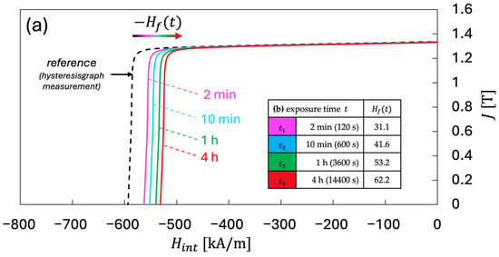
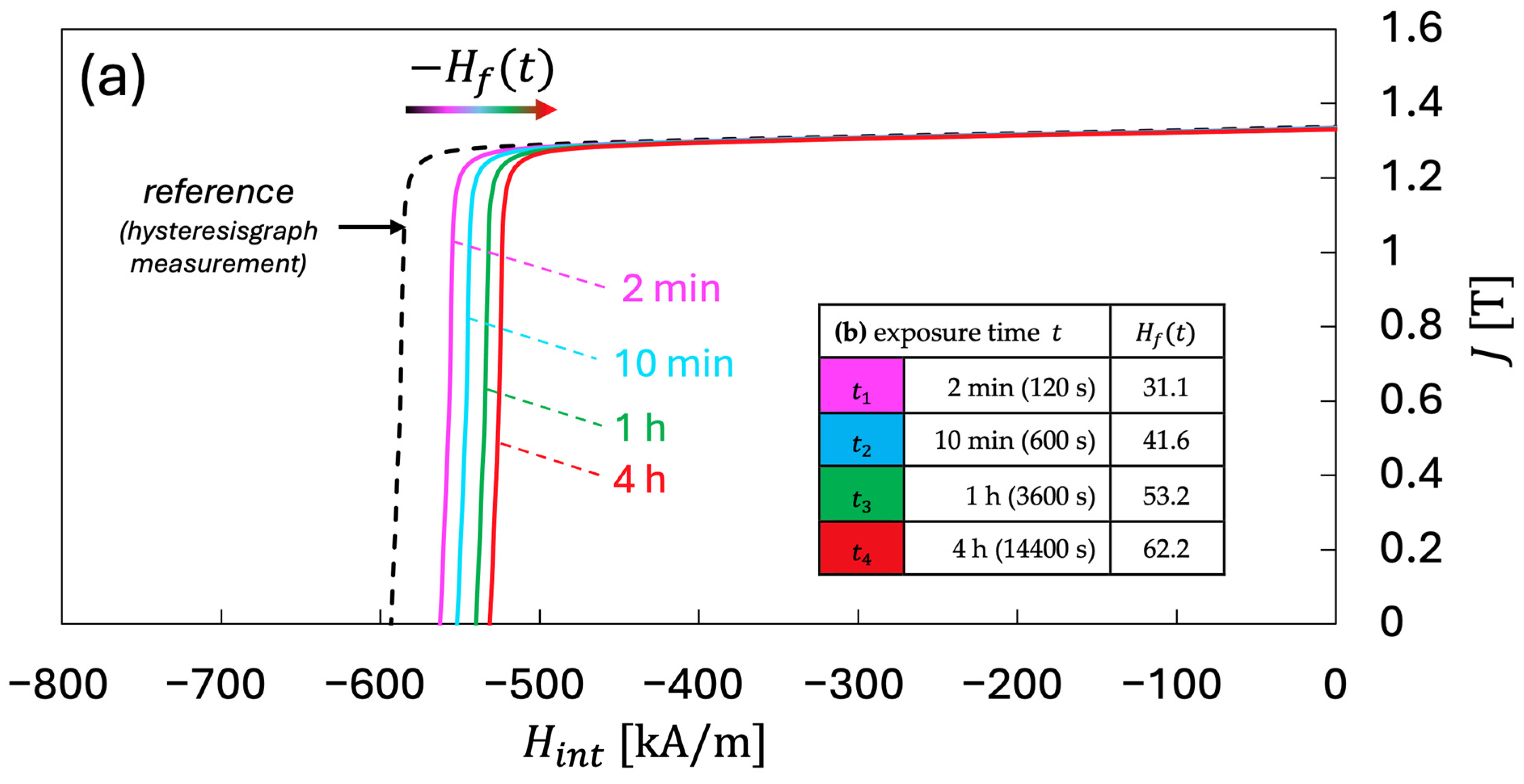
Figure 4 shows the resulting time-shifted demagnetization curves at 80 °C. The initial reference curve is based on hysteresisgraph measurements, which are assumed as $t_0=$ 1 s. Using a viscosity parameter of $S_v=$ 6.5 kA/m, the corresponding fluctuation field values as a function of time result in: $H_f\left(t_1=2 \mathrm{m}\mathrm{i}\mathrm{n}\right)$ = 31.1 kA/m, $H_f\left(t_2=10 \mathrm{m}\mathrm{i}\mathrm{n}\right)$ = 41.6 kA/m, $H_f(t_3=1 \mathrm{h})$= 53.2 kA/m, and $H_f(t_4=4 \mathrm{h})$ = 62.2 kA/m.

Figure 4. (a) $J\left(H\right)$ hysteresis curves at 80 °C with different exposure times: $t_0$ (reference curve from hysteresisgraph measurement, relaxation time $t_0$ = 1 s, black), 2 min (pink), 10 min (bright blue), 1 h (green), and 4 h (red). The curves were horizontally shifted relative to the reference sample curve using the fluctuation field according to Equation (6), resulting in reduced effective coercivity values that represent the different exposure times (time-dependent demagnetization). (b) Shows the resulting fluctuation field values corresponding to these exposure times.

Since time-dependent magnetization losses occur in the irreversible region beyond the knee point, simple curve shifts according to Equation (6) can falsely suggest polarization losses in the linear reversible region, where time-dependency is negligible.

Therefore, the procedure for constructing the curves in Figure 4 is:

• Determine the initial slope at H = 0 and subtract a straight line with this slope from the $J\left(H\right)$ or $B\left(H\right)$ curves; this results in curves that are horizontal at $H$ = 0. This procedure avoids effects of the fluctuation field correction in the reversible part of the curves, where nearly no time dependency occurs.
• Replace the $H$ values for each point by $H-H_f\left(t\right)$ (Equation (6)), thus shifting the curves to the right.
• Reintroduce the linear slope removed in the first step.

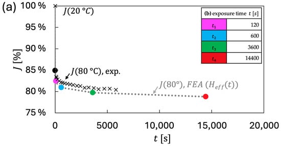
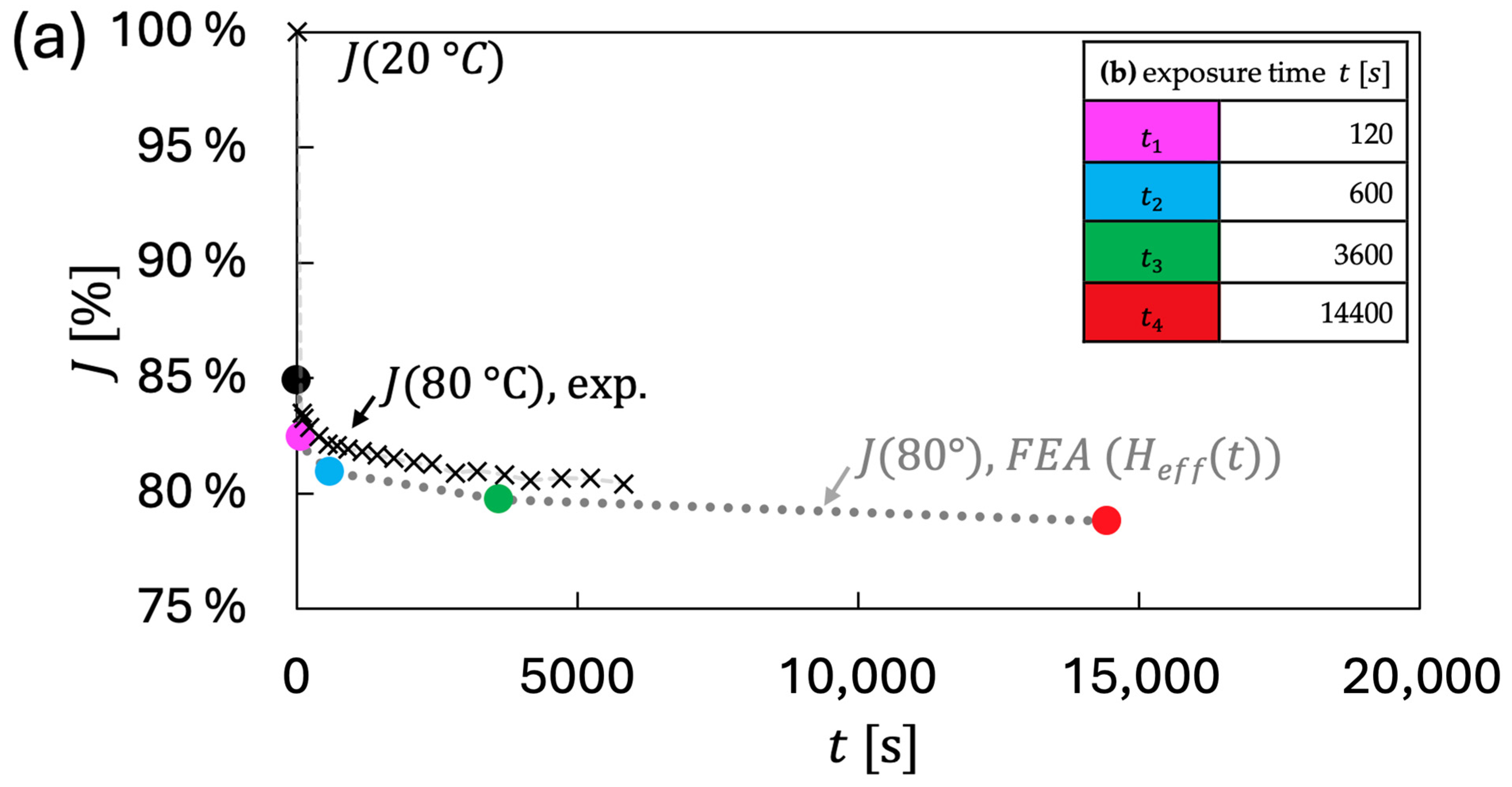
To validate this procedure, the $J\left(H\right)$ curves from Figure 4 were implemented in FE software (Simcenter Magnet 2023) [15] and assigned to a cuboid sample (20 × 10 × 5 mm³) for 20 °C and 80 °C, as well as for 80 °C, using the shifted demagnetization curves (representing the corresponding exposure times). The temperature of 80 °C was chosen to exemplify the method with a sample working point within the irreversible region around the $H_{D5}$ field strength. This method can be applied at other temperatures, provided that the working point lies within the irreversible region to exhibit pronounced time-dependent demagnetization. The extracted simulated polarization values were compared with experimental long-term open-circuit measurements using a rotating sample in a Helmholtz coil measurement setup, as described in detail in previous work in Ref. [23]. The experiments were performed under controlled temperature conditions over 4 h, revealing the time-dependent polarization decrease $J(T,t)$(dashed lines in Figure 5). To account for differing initial polarization levels between simulation and experiment, both results are presented as differential percent polarization in Figure 5. Here, the comparison reveals good agreement, with only a small offset of less than 1.5%. This validates the proposed theoretical approach of shifting $J\left(H\right)$ curves by $H_f\left(t\right)$, thereby enabling a simple and effective method for considering time-dependent magnetic losses in numerical calculation tools.

Figure 5. Comparison of the theoretical (simulated) approach using shifted $J(H,t)$ curves with experimental long-term measurements. (a) Theoretical prediction based on an FEA simulation of a cuboid sample (20 × 10 × 5 mm³) using the shifted $J(H,t)$ curves from Figure 4. The resulting colored $J$ values correspond to the respective curves at the specific exposure times $t$ listed in (b) and show good agreement with the experimental $J(T,t)$ measurement of an N52 sample at 80 °C, conducted in a Helmholtz coil setup with time-resolved magnetization measurement (see text).

The presented procedure for relating time-dependency in FEA simulations illustrates a basic methodology that can be applied for several applications with static field and temperature loads. However, its applicability to, for example, electric motor simulations, is challenging due to the transient, time-varying field loads within electric motors.

5. Conclusions

Unlike the magnetic viscosity $S$, which strongly depends on the exact field and temperature conditions and thus complicates practical comparisons, the viscosity parameter $S_v$ is less affected by application-specific conditions and provides a robust metric for assessing time-dependent magnetization losses in permanent magnets. Its magnitude increases with sample coercivity, typically ranging from about 4 kA/m for low-coercivity materials to 8 kA/m for high-coercivity materials, reflecting the resistance of the material to long-term demagnetization.

Based on Néel’s fluctuation-field concept, $S_v$ enables prediction of time-dependent magnetization decay by relating effective field fluctuations to their position on the material’s $J\left(H\right)$ curve. This supports both simplified evaluations using $J\left(H\right)$ curves and advanced numerical calculations, including finite element analysis, making it suitable for practical system design considerations. This procedure is not restricted to NdFeB magnets and can be applied to other hard magnetic materials exhibiting time-dependent demagnetization behavior.

The practical evaluation of permanent magnets can proceed as follows:

• Define the maximum field, temperature, and operating time.
• Determine the fluctuation field from magnetic viscosity measurements or reference values (Table 2). For typical samples, an additional 160 kA/m corresponds approximately to 10 years.
• Calculate the effective field $H_{eff}$ a s the sum of the application field and the fluctuation field.
• Evaluate the position of ${\mathit{H}}_{\mathit{e}\mathit{f}\mathit{f}}$${\mathit{H}}_{\mathit{e}\mathit{f}\mathit{f}}$on the material’s $\mathit{J}\left(\mathit{H}\right)$$\mathit{J}\mathit{\left(}\mathit{H}\mathit{\right)}$curve. If $H_{eff}$ remains within the linear reversible region, a stable polarization state with minor irreversible losses can be expected. In contrast, $H_{eff}$ values beyond the knee region indicate a high risk of irreversible demagnetization, requiring either the selection of a higher-coercivity-material grade or a modification of the system design, for example, by reducing the demagnetization factor $N$.

Step 4 can also be incorporated into numerical calculations, providing a simple method to account for time-dependent effects in magnetic system design. This procedure can, in principle, also be applied to electric motor simulations to provide a rough estimation of worst-case scenarios, where the material data curves are shortened according to the expected operational lifetime.

Overall, this methodology links material properties with practical design criteria and simulation tools, enabling improved material selection, reduced overdimensioning, and enhanced long-term reliability of permanent magnet systems.

References

- Brauer, J.R. Magnetic Actuators and Sensors, 2nd ed.; Wiley-IEEE Press: Hoboken, NJ, USA, 2014; ISBN 978-1-118-50525-0. [Google Scholar]
- Gutfleisch, O.; Willard, M.A.; Brück, E.; Chen, C.H.; Sankar, S.G.; Liu, J.P. Magnetic Materials and Devices for the 21st Century: Stronger, Lighter, and More Energy Efficient. Adv. Mater. 2011, 23, 821–842. [Google Scholar] [CrossRef] [Scilit] [PubMed]
- Coey, J.M.D. Permanent Magnet Applications. J. Magn. Magn. Mater. 2002, 248, 441–456. [Google Scholar] [CrossRef] [Scilit]
- Clegg, A.G.; Coulson, I.M.; Hilton, G.; Wong, H.Y. The Temperature Stability of NdFeB and NdFeBCo Magnets. IEEE Trans. Magn. 1990, 26, 1942–1944. [Google Scholar] [CrossRef] [Scilit]
- Ruoho, S.; Haavisto, M.; Takala, E.; Santa-Nokki, T.; Paju, M. Temperature Dependence of Resistivity of Sintered Rare-Earth Permanent-Magnet Materials. IEEE Trans. Magn. 2010, 46, 15–20. [Google Scholar] [CrossRef] [Scilit]
- Skomski, R.; Zhou, J.; Kirby, R.D.; Sellmyer, D.J. Magnetic Aging. MRS Proc. 2005, 887, 8870707. [Google Scholar] [CrossRef] [Scilit]
- Street, R.; Woolley, J.C. A Study of Magnetic Viscosity. Proc. Phys. Soc. A 1949, 62, 562. [Google Scholar] [CrossRef] [Scilit]
- Gaunt, P. Magnetic Viscosity and Thermal Activation Energy. J. Appl. Phys. 1986, 59, 4129–4132. [Google Scholar] [CrossRef] [Scilit]
- Néel, L. Théorie du traînage magnétique des substances massives dans le domaine de Rayleigh. J. Phys. Radium 1950, 11, 49–61. [Google Scholar] [CrossRef] [Scilit]
- Barbier, J.-C. Le Trainage Magnétique de Fluctuation. Ann. Phys. 1954, 12, 84–140. [Google Scholar] [CrossRef] [Scilit]
- Kronmüller, H.; Fähnle, M. Micromagnetism and the Microstructure of Ferromagnetic Solids; Cambridge Studies in Magnetism; Cambridge University Press: Cambridge, UK, 2003; ISBN 978-0-521-33135-7. [Google Scholar]
- Givord, D.; Tenaud, P.; Viadieu, T.; Hadjipanayis, G. Magnetic Viscosity in Different Nd-Fe-B Magnets. J. Appl. Phys. 1987, 61, 3454–3456. [Google Scholar] [CrossRef] [Scilit]
- Street, R.; Day, R.K.; Dunlop, J.B. Magnetic Viscosity in NdFeB and SmCo5 Alloys. J. Magn. Magn. Mater. 1987, 69, 106–112. [Google Scholar] [CrossRef] [Scilit]
- Crew, D.C.; McCormick, G.; Street, R. Measurement of Magnetic Viscosity in NdFeB. IEEE Trans. Magn. 1996, 32, 4356–4358. [Google Scholar] [CrossRef]
- Simcenter MAGNET; Siemens Digital Industries Software: Plano, TX, USA.
- Ansys Maxwell; Ansys Inc.: Canonsburg, PN, USA.
- Chen, F. Recent Progress of Grain Boundary Diffusion Process of Nd-Fe-B Magnets. J. Magn. Magn. Mater. 2020, 514, 167227. [Google Scholar] [CrossRef] [Scilit]
- Bance, S.; Fischbacher, J.; Kovacs, A.; Oezelt, H.; Reichel, F.; Schrefl, T. Thermal Activation in Permanent Magnets. JOM 2015, 67, 1350–1356. [Google Scholar] [CrossRef] [Scilit]
- Brown, W.F. Thermal Fluctuations of a Single-Domain Particle. Phys. Rev. 1963, 130, 1677–1686. [Google Scholar] [CrossRef] [Scilit]
- Hilzinger, R.; Rodewald, W. Magnetic Materials: Fundamentals, Products, Properties, and Applications; Publicis: Paris, France, 2013; ISBN 978-3-89578-352-4. [Google Scholar]
- Lanz, M.; Martinek, G.; Kresse, T.; Schneider, G.; Goll, D. Magnetic Viscosity Characterization of Fe–Nd–B Permanent Magnets Using a Novel Measurement Approach. IEEE Transactions on Magnetics 2025, 61, 1–5. [Google Scholar] [CrossRef] [Scilit]
- Kresse, T.; Martinek, G.; Schneider, G.; Goll, D. The Field-Dependent Magnetic Viscosity of FeNdB Permanent Magnets. Materials 2024, 17, 243. [Google Scholar] [CrossRef] [Scilit]
- Lanz, M.; Martinek, G.; Kresse, T.; Georgiadis, A.; Schneider, G.; Goll, D. Application-Oriented In-Situ Testing Methods for Permanent Magnet Characterization. In Proceedings of the SMSI 2025 Conference—Sensor and Measurement Science International, Nürnberg, Germany, 6–8 May 2025; AMA Service GmbH: Wunstorf, Germany, 2025; pp. 327–328. [Google Scholar] [CrossRef] [Scilit]
- IEC 60404-8-1; Magnetic Materials—Part 8-1: Specifications for Individual Materials—Magnetically Hard Materials. International Electrotechnical Commission: Geneva, Switzerland, 2015.
- Bekir, W.; Messal, O.; Benabou, A. Permanent Magnet Non-Linear Demagnetization Model for FEM Simulation Environment. IEEE Trans. Magn. 2022, 58, 1–5. [Google Scholar] [CrossRef] [Scilit]
- Dennison, E.J. The Hysteresisgraph as a Quality Control Tool. In Proceedings of the Electrical/Electronics Insulation Conference; IEEE: Chicago, IL, USA, 1993; pp. 221–227. [Google Scholar]
- Basso, V.; Beatrice, C.; LoBue, M.; Tiberto, P.; Bertotti, G. Study of the Connection between Hysteresis and Thermal Relaxation in Magnetic Materials. Phys. Rev. B 2000, 61, 1278–1285. [Google Scholar] [CrossRef] [Scilit]
- Sun, H.; Pang, W.; Street, R. Field Rate Measurement of Time-Dependent Magnetic Phenomena. IEEE Trans. Magn. 2000, 36, 3360–3362. [Google Scholar] [CrossRef] [Scilit]
Disclaimer/Publisher’s Note: The statements, opinions and data contained in all publications are solely those of the individual author(s) and contributor(s) and not of MDPI and/or the editor(s). MDPI and/or the editor(s) disclaim responsibility for any injury to people or property resulting from any ideas, methods, instructions or products referred to in the content. |
© 2026 by the authors. Licensee MDPI, Basel, Switzerland. This article is an open access article distributed under the terms and conditions of the Creative Commons Attribution (CC BY) license.