Accelerating and Improving the Accuracy of Parameter Calibration in a Phenomenological Crystal Plasticity Model Through High-Volume Machine Learning Simulations

Abstract

Phenomenological crystal plasticity (CP) models are widely used in Integrated Computational Materials Engineering (ICME) to link microstructural features with engineering-scale mechanical behaviour. Their practical use, however, is limited by the high computational cost of physics-based simulations and the labour-intensive nature of parameter calibration, challenges that are amplified in additively manufactured materials with location-dependent properties. To address these obstacles, we first developed deep neural network (DNN) surrogate models of physics simulations to predict the stress–strain response of an additively manufactured AlSi10Mg alloy. Twenty-five experimentally derived scenarios (five microstructures × five sets of grain orientations) were used for training 25 separate DNNs, with datasets for validated material behaviour generated using the Düsseldorf Advanced Material Simulation Kit (DAMASK) platform and a Fast Fourier Transform (FFT)-based solver. Once trained, the DNNs produced stress–strain curves almost instantaneously, enabling an exhaustive grid-search exploration of a vast parameter space. Our approach yielded significant efficiency gains, which were comprehensively quantified. The best-fit CP parameters obtained through this approach are expected to be more accurate than those derived from conventional trial-and-error calibration, which is restricted to a limited number of candidate values. In addition, the minimum number of CP-FFT simulations required to train the DNNs with sufficient accuracy was identified, reducing the need for costly physics simulations in future studies. The proposed framework enhances the practical utility of CP models for simulation-informed materials engineering and optimisation and is broadly applicable to parameter identification in phenomenological models of other domains.

1. Introduction

Integrated Computational Materials Engineering (ICME) is a multidisciplinary approach that seeks to unify materials science, engineering, and computational modelling to accelerate the design and optimisation of materials, components, and processes. By linking process, structure, property, and performance through predictive models, ICME enables more efficient innovation cycles and tailored material solutions across diverse industries. It is well established that engineering-scale properties, which govern part-level material performance, are fundamentally influenced by microstructures that belong to much smaller length scales. This disparity in scales poses a significant challenge for modelling the structure–property relationship in ICME using purely physics-based models with sufficient resolution to account for microstructural influences. Fortunately, phenomenological crystal plasticity (CP) models are well suited to linking microstructural features to continuum-scale stress–strain behaviour while capturing realistic anisotropic (i.e., heterogeneous directional) responses. For instance, for highly anisotropic additively manufactured (AM) materials with location-dependent microstructures and properties, high-fidelity CP models based on realistic microstructure predictions can expedite part qualification through digital certification pathways and reduce reliance on costly, wasteful destructive testing. However, CP models remain underutilised to date owing to the high computational burden of simulations and the laborious nature of trial-and-error parameter calibration methods [1,2], which also do not necessarily guarantee global optimality in parameter extraction. The challenges are amplified for AM materials, which exhibit location-dependent microstructures, since the calibration procedure must be repeated at various points to obtain a detailed map of their properties. Therefore, strategies that accelerate model calibration are highly valued, as the efficiency gains they deliver would facilitate the broader adoption of CP models in real-world applications involving materials design and optimisation. The present work aimed to explore an approach that leverages fast-solving machine learning (ML) models to expedite CP simulations and, consequently, parameter discovery.

Robust calibration requires evaluating numerous parameter sets to identify the best-performing set according to an error metric. ML models provide a powerful means to accelerate model calibration, thanks to their ability to process large datasets efficiently and deliver results in seconds. By developing fast-solving ML surrogates of CP simulations, it becomes feasible to rapidly generate and evaluate a prodigious amount of stress–strain curves (SSCs) for different CP parameter sets. Such exploration of an extensive parameter space substantially increases the likelihood of identifying a more accurate parameter set than conventional procedures, thereby improving the predictive performance of CP models.

A limited number of works that reported the creation of ML surrogates of CP simulations for CP parameter calibration exist in the open literature, e.g., [3,4,5,6,7,8,9,10,11,12,13,14,15,16,17,18,19,20,21]. The ML surrogates efficiently approximated computationally expensive CP simulations. Researchers developed surrogate models using algorithms such as Artificial Neural Networks (ANNs), Deep Neural Networks (DNNs), Bayesian Neural Networks (BNNs), Feedforward Neural Networks (FNNs), Support Vector Regression (SVR), Random Forest (RF), and Gaussian Processes (GPs). These models were trained on data generated by detailed CP simulations, primarily using the Finite Element Method (CP-FEM), the Fast Fourier Transform (CP-FFT), or the Viscoplastic Self-Consistent (CP-VPSC) approach. These surrogates significantly reduced computational time while maintaining reasonable accuracy. However, none of the studies listed above quantified the time savings achieved by employing ML surrogates to identify best-fit parameter values relative to a conventional trial-and-error calibration process, nor did they explore an exhaustive space of candidate parameter sets for additively manufactured AlSi10Mg, a widely used alloy. Furthermore, no prior work has established the minimum number of datasets required to train a DNN with adequate accuracy, which is essential for minimising the number of costly physics-based simulations needed to generate those datasets.

Our work was designed to address the research gaps outlined above. Deep neural network (DNN) surrogate models were trained using results from 2D CP simulations for various statistically equivalent microstructure/grain orientation combinations of a popular AM alloy. The Fast Fourier Transform (FFT)-based spectral solution method was used to obtain engineering SSCs for comparison with the experimental curves, with the root mean square error (RMSE) as the metric. The DNNs reproduced the SSCs almost instantaneously for 25 experimentally derived scenarios (5 microstructures × 5 sets of grain orientations) of the AlSi10Mg alloy produced via laser powder bed fusion (L-PBF) AM. Additionally, 104,060,401 candidate parameter sets were evaluated for each scenario in a relatively short time to identify the best-fitting set.

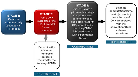
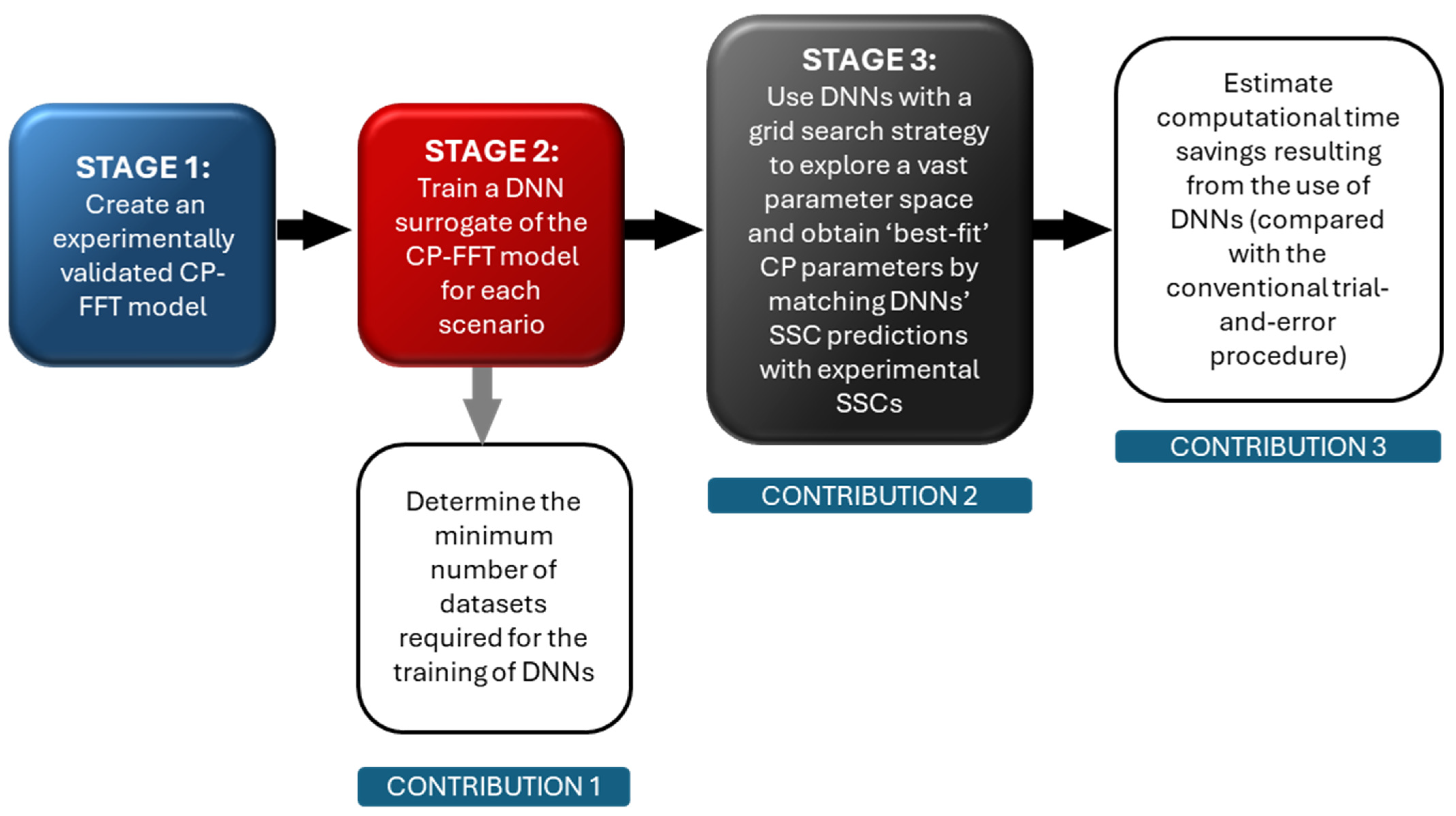
The primary focus of this article is quantifying the efficiency gains achieved through the DNN-accelerated framework. Accordingly, the details of the CP-FFT model construction, DNN training procedures, and Grid Search Scheme (GSS) implementation are presented only in summary form here; however, comprehensive descriptions are available in open-access Refs. [22,23] accessible through public repositories such as the CSIRO Research Publications Repository and ResearchGate. The remainder of the manuscript is organised around the three sequential stages of the research we followed (Figure 1). Stage 1 involved developing an experimentally validated CP-FFT model. Stage 2 focused on creating DNN surrogates of the CP-FFT model across 25 scenarios. In Stage 3, an automated GSS that mimicked the manual trial-and-error procedure was implemented. The presentation of results, a detailed discussion, and the drawing of final conclusions follow these stages. Contributions made by the current investigation are also highlighted in Figure 1.

Figure 1. Workflows associated with the current investigation and contributions of this study.

2. Stage 1: Creating a Validated CP-FFT Model

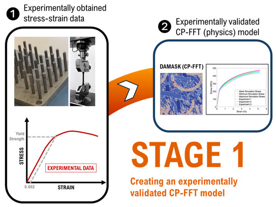
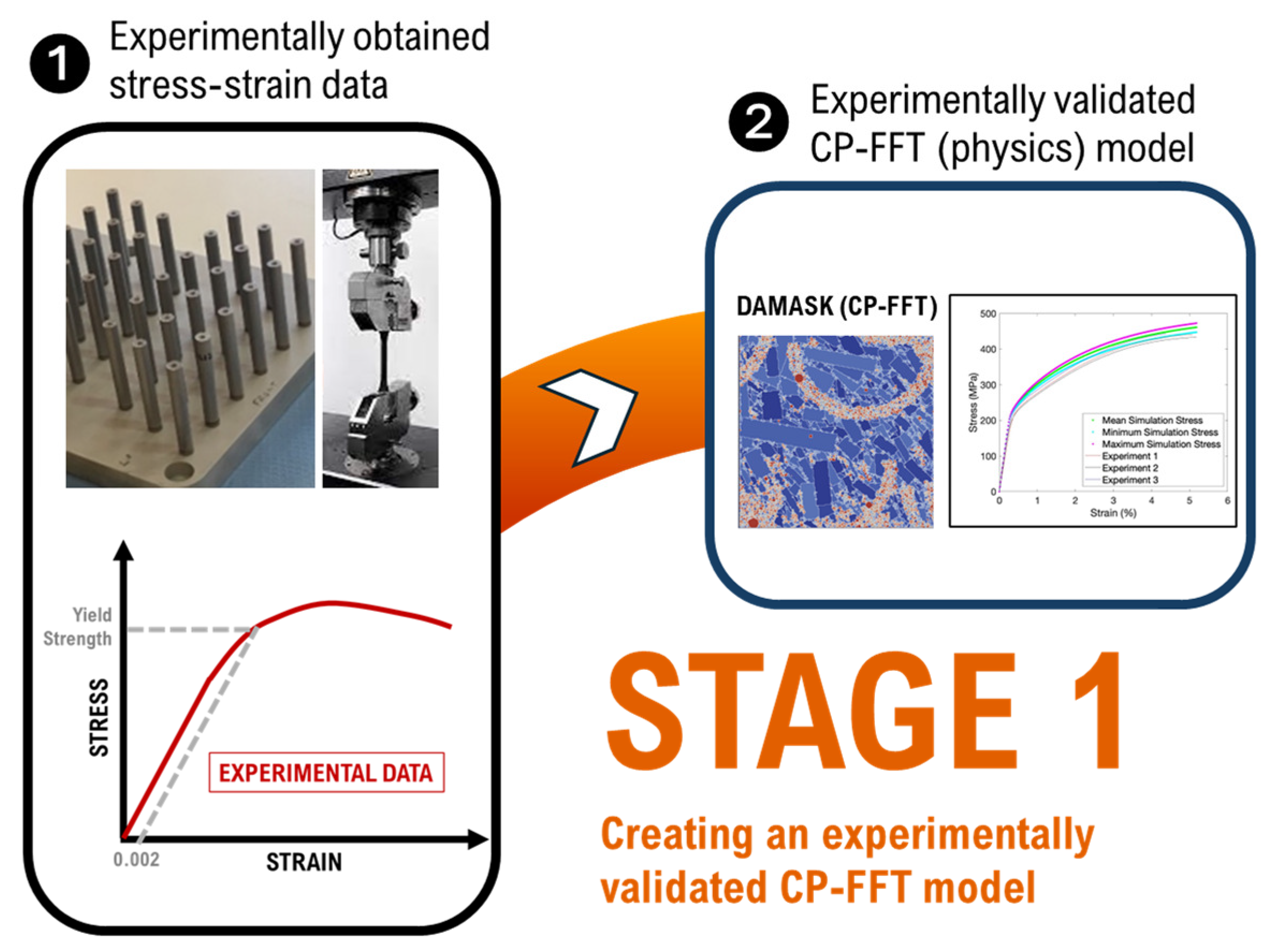
Stage 1 focused on developing an experimentally validated CP-FFT model (Figure 2) using the Düsseldorf Advanced Material Simulation Kit (DAMASK) (Max-Planck-Institut für Nachhaltige Materialien GmbH, Munich, Germany) [24]. The following text outlines key components, such as the CP constitutive model, and introduces its parameters that require calibration using experimental data. The validation process for the model’s SSC predictions is also discussed. Additional details, such as the microstructures, grain orientations, and the development of Statistically Equivalent Representative Volume Elements (SERVEs), are readily available in an open-access document [22].

Figure 2. Stage 1 of the work aimed to develop an experimentally validated CP-FFT physics model to predict the stress–strain behaviour of AM AlSi10Mg.

2.1. Constitutive Models and Adjustable Parameters

2.1.1. CP Constitutive Model and the Four Tuneable Parameters

When mechanical loading causes a material to exceed its yield point, dislocations move, leading to permanent (plastic) deformation. Dislocations are defects within the orderly crystal lattice structures found in metals, and their movement under stress allows the material to deform without fracturing. These crystallographic deformation mechanisms are highly dependent on crystallographic orientation [25,26]. Phenomenological CP models are commonly used to describe the plastic deformation of metal alloy systems, including AlSi10Mg, and are described briefly here. The constitutive equations at a slip system level contain a slip rate equation and a hardening law to describe deformation under loading [27]. To begin, the deformation gradient F is decomposed into elastic and plastic components:

F = F^eF^p,

(1)

where F^e and F^p are the elastic and plastic components of the deformation gradient, respectively. The elastic deformation gradient F^e is related to the elastic Green-Lagrange strain E via the relation:

E = ((F^e)^T F^e − I)/2

(2)

where I is the second-order identity tensor. The elastic strain E is used to calculate the second Piola-Kirchoff stress S using a generalised Hooke’s law:

S = C:E,

(3)

where C is the elasticity tensor calculated using the single-crystal elasticity model described in [22]. The plastic deformation gradient F^p at any time t can be calculated in terms of the plastic velocity gradient L^p [28]:

F^p(t) = (I − ∆tL^p(t))⁻¹F^p(t₀).

(4)

where L^p is the plastic velocity gradient. L^p can be calculated using slip system kinematics as follows [14]:

$$\begin{array}{cc}{\mathbf{L}}^p=\hfill & {\displaystyle \sum _{\alpha =1}^{Ns}}{\dot{\gamma }}_{\alpha }({\widehat{\mathit{s}}}^{\mathsf{\alpha }}\otimes {\widehat{\mathit{n}}}^{\mathsf{\alpha }}),\hfill \end{array}$$

(5)

where N_s denotes the number of slip systems α present in the crystallographic lattice, $\dot{\gamma }$_α denotes the slip rate, $\widehat{\mathit{s}}$^α and $\widehat{\mathit{n}}$^α are the unit vectors parallel and normal to the slip direction, respectively, and ⊗ indicates the tensor product. Hence, to calculate the plastic velocity gradient L^p and, subsequently, the plastic deformation, F^p, we require constitutive laws for the slip rate $\dot{\gamma }$_α.

The slip rate equation essentially relates the applied stress to the plastic strain rate, thereby defining the rate-dependent nature of plastic deformation. We calculate the slip rate $\dot{\gamma }$_α for the AlSi composite grains (slip system a) using the phenomenological CP model of Hutchinson [29], which has been shown to be suitable for AM AlSi10Mg systems [14] comprising an FCC crystal structure:

$${\dot{\gamma }}_{\alpha }= {\dot{\gamma }}_{0 }{\left|{\displaystyle \frac{\tau \alpha }{{\tau }_{\alpha }^c}}\right|}^m\mathrm{sgn}\left({\tau }_{\alpha }\right)$$

(6)

where $\dot{\gamma }$₀ denotes the reference shear rate, m denotes the power law exponent of rate-sensitivity, ${\tau }_{\alpha }^c$ denotes the slip resistance, and τ_α denotes the resolved shear stress.

To complete the phenomenological CP model, we must define the hardening law. This law describes the rate at which the slip resistance ${\tau }_{\alpha }^c$ evolves with accumulated plastic deformation, thereby determining how the material’s strength changes as it deforms. It captures the effects of dislocation interactions and other microstructural mechanisms that increase resistance to further deformation, e.g., strain hardening. We calculate the evolution of slip resistance as:

$${\dot{\tau }}_{\alpha }^c=h_0\times \sum _{\beta =1}^{N_s}\left|\dot{{\gamma }_{\beta }}\right|{(1-{\displaystyle \frac{{\tau }_{\beta }^c}{{\tau }_{\beta }^{\infty }}})}^a{q}_{\alpha \beta }$$

(7)

where h₀ is the overall hardening parameter, similarly a is a slip hardening parameter, q_αβ is the slip system interaction parameter between slip systems a and b, and τ_β^∞ is a slip system-specific saturation value for slip resistance. Hereinafter, τ_β^∞ is referred to as τ_∞ for convenience. Additionally, the initial condition for τ_β^c is prescribed as τ_β^c|_{t = 0} = τ₀.

In the present work, we sought the optimal values of the parameters a, h₀, τ₀, and τ_∞ associated with the alloy grains, as they exert the greatest influence on the shape of SSCs. While parameter m, which encapsulates the influence of strain rate sensitivity, was also tuneable, we used a constant value for this parameter in our work because our experiments were conducted at a single strain rate across all specimens. Furthermore, m did not have a significant impact on SSC shape in our CP-FFT simulations. Thus, we adjusted only the parameters in the equation for the evolution of slip resistance (Equation (7)).

2.1.2. Dilatational Plasticity Model for the Porosity

Since our material contained pores (see [22]) in addition to the alloy grains, the deformation of pores was also accounted for. We note that it is common to use a simple elastic model for the porosity (e.g., [14]) in which the pores are modelled as soft, purely elastic regions. However, we found that these simple elastic models led to convergence issues with the spectral solver at higher porosity levels. In such cases, the dilatational plasticity model of Maiti and Eisenlohr [30] is better suited for modelling void-like regions (e.g., pores), and, to the best of our knowledge, we are the first to implement the dilatational plasticity model for AM microstructures. While a detailed explanation of this model may be found in Ref. [30], we provide the most relevant equations below. In this model, the deformation gradient F for the pores is decomposed into elastic, intermediate, and plastic components as:

F = F^eFⁱF^p.

(8)

This requires the calculation of the velocity gradient Lⁱ for the intermediate deformation gradient Fⁱ as follows:

$${\mathbf{L}}^i={\dot{ϵ}}_0{\left({\displaystyle \frac{p}{Mg}}\right)}^m\mathrm{I}$$

(9)

The evolution of deformation resistance is given as:

$$\dot{g}=M{\dot{ϵ}}_0{\left({\displaystyle \frac{\sqrt{3J_2}}{Mg}}\right)}^a{h}_0{(1-{\displaystyle \frac{g}{g_{\infty }}})}^n$$

(10)

where a, h₀, m, g (equivalent to τ₀ at time = 0), and g_∞ (equivalent to τ_∞) are adjustable parameters, p is the hydrostatic pressure which can be calculated from the stress tensor corresponding to the intermediate configuration, n is the stress exponent, M is the Taylor factor, J₂ is the second invariant of the deviatoric second Piola-Kirchoff stress. I is the second-order identity tensor (as defined earlier).

Unlike for the alloy phase, the CP parameter values for the pore regions were left unchanged, as the limited presence of the pores in the material (see [22]) rendered their influence on mechanical behaviour negligible.

2.2. Validation of CP-FFT Model Predictions Against the Ground-Truth

2.2.1. Generation of the Ground-Truth: Experimental Details

Part Geometry and Tensile Specimen Dimensions

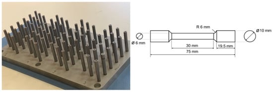
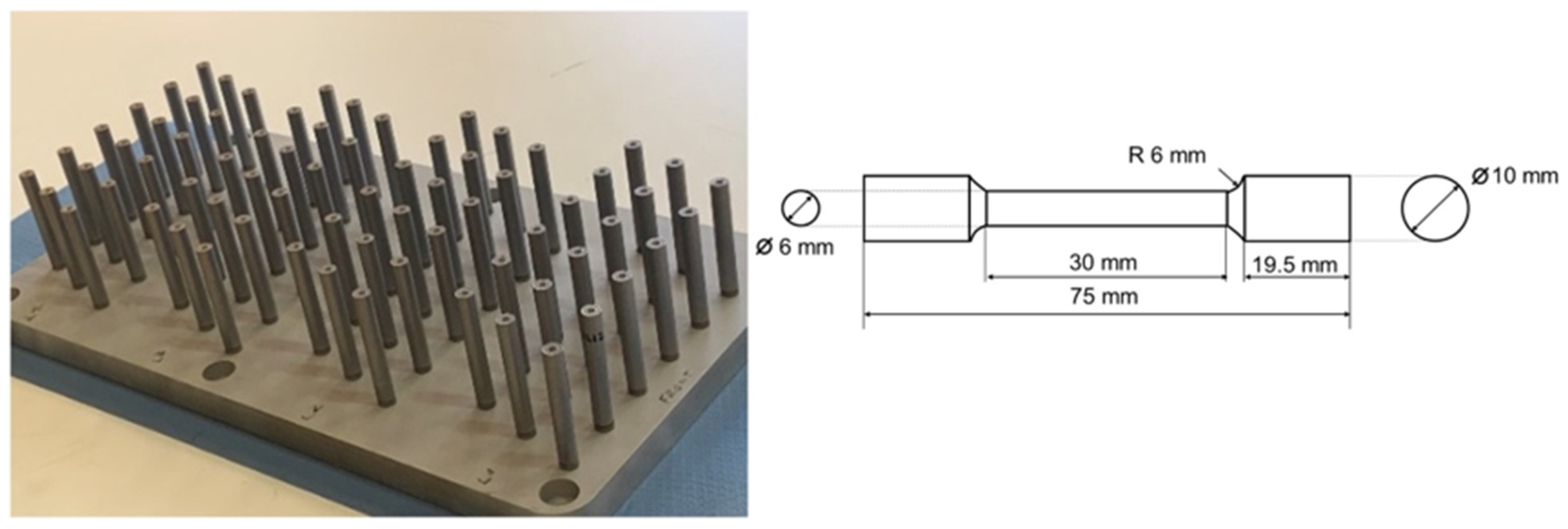
Cylindrical parts were built using the L-PBF technology to obtain the tensile specimens for testing (see Figure 3). These parts were built to a height of slightly above 75 mm before the specimens were machined to ASTM Standard E8/E8M-16a (ASTM International, West Conshohocken, PA, USA).

Figure 3. The cylindrical parts built using L-PBF are shown in the as-built condition (left). Tensile specimens (right) were machined out of these for testing.

Material and AM Process Parameters

The AlSi10Mg powder (composition in Table 1) was supplied by Nikon SLM Solutions AG (Lübeck, Germany) with a size distribution of 20–63 µm. The samples were manufactured using an SLM^® 500 HL and printed directly onto an Al build plate preheated to 150 °C, without support structures. The processing parameters were as follows: laser power 350 W, scan speed 1135 mm/s, hatch spacing 0.19 mm, layer thickness 0.03 mm, spot diameter 0.08 mm, and a stripe-scanning strategy with 67° rotation after every layer. The samples were detached from the build plate using wire electro-discharge machining (EDM).

Table 1. Composition of AlSi10Mg alloy by weight (%) measured using inductively coupled plasma atomic emission spectroscopy.

Al	Si	Mg	Fe	Mn	Co	Ti	Cu	Zn
Balance	10.3	0.32	0.18	0.15	0.10	0.025	0.01	<0.01

Microstructure Imaging

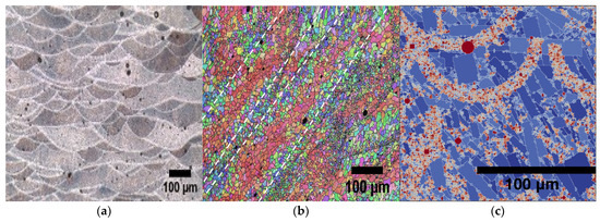
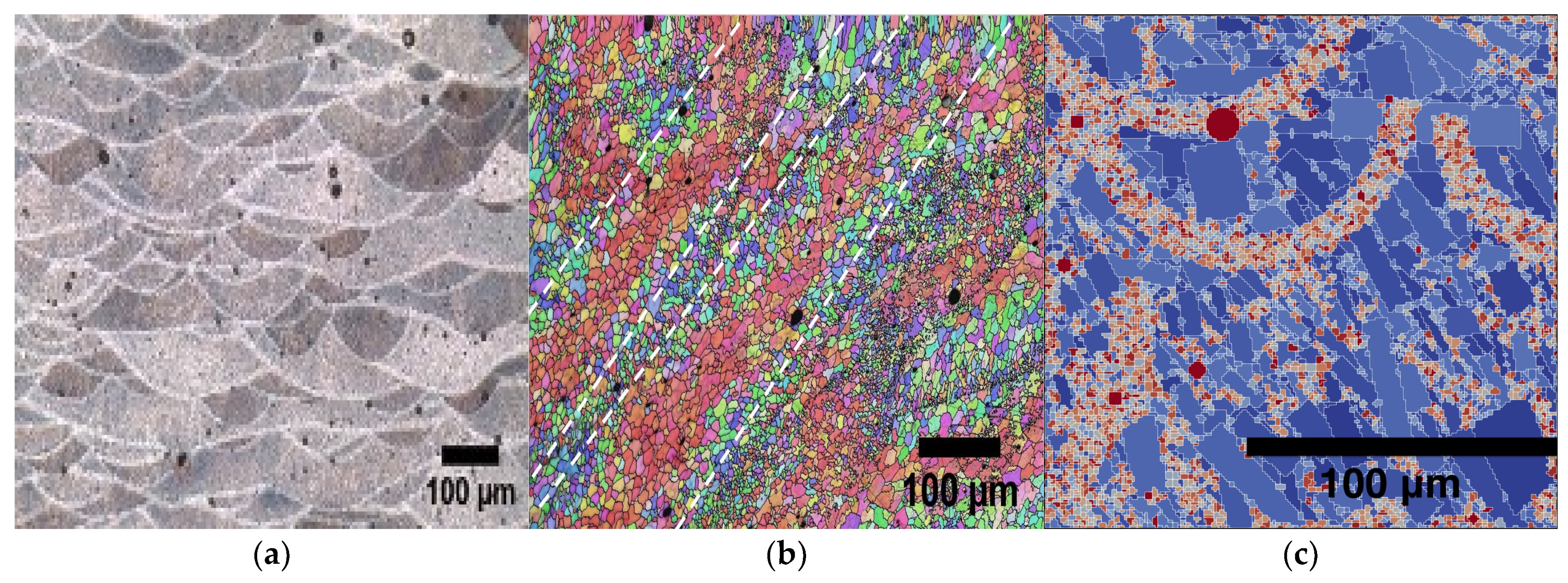
Cross-sections from vertical planes in the gauge length regions of untested tensile pieces were cut and mounted in electrically conductive resin. Because these cross-sections were obtained from parts equivalent to those used for tensile testing, the microstructures were representative. Mounted samples were ground and polished through multiple steps using a Struers polishing machine. Samples were ground on a 220-grit SiC pad followed by an 800-grit SiC pad and a 9 µm diamond suspension. Subsequently, the samples were polished with a 3 µm diamond suspension, followed by polishing with a 0.04 µm oxide polishing suspension (OPS). For electron backscatter diffraction (EBSD) analysis, polished samples were further polished on a Struers vibro-polisher machine using 0.04 µm OPS for 4 h. In this work, we distinguished between melt pool centres (MPCs) and melt pool boundaries (MPBs) (see [22]). Therefore, to investigate their respective volume fractions, the samples were etched in Keller’s reagent (2.5 mL HNO₃, 1.5 mL HCl, 1 mL HF, and 95 mL water) for 25 s prior to imaging. Optical microscopy was performed using a Leica DM2500 (Leica Microsystems, Wetzlar, Germany). A JEOL 7200 F scanning electron microscope (SEM) (Tokyo, Japan) was utilised for high-resolution microscopy and EBSD analysis. A high-precision Oxford detector was installed on the SEM for EBSD pattern collection, and AZtecCrystal software was used to analyse and quantify the collected patterns. A representative microstructure and a SERVE used in CP-FFT calculations are shown in Figure 4 [22].

Figure 4. A typical microstructure (including porosity). (a) optical microscopy image; (b) EBSD image; and (c) a representative SERVE used in the CP-FFT computations. Further details are available in Ref. [22].

Mechanical: Testing to Obtain Ground-Truth SSCs

Tensile tests were conducted on an Instron 50 kN uniaxial testing machine (Illinois Tool Works, Inc., Glenview, IL, USA) using samples shown in Figure 3 (right). The tests were conducted at 5 mm/min. Three samples were tested to generate the SSCs used as ground-truth for the current work. These were sufficient to demonstrate that CP parameters of AM alloys can be obtained without resorting to the destructive testing of several expensive AM parts.

2.2.2. Validation of CP-FFT Model Predictions

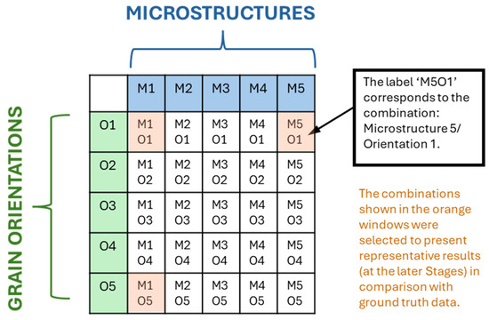
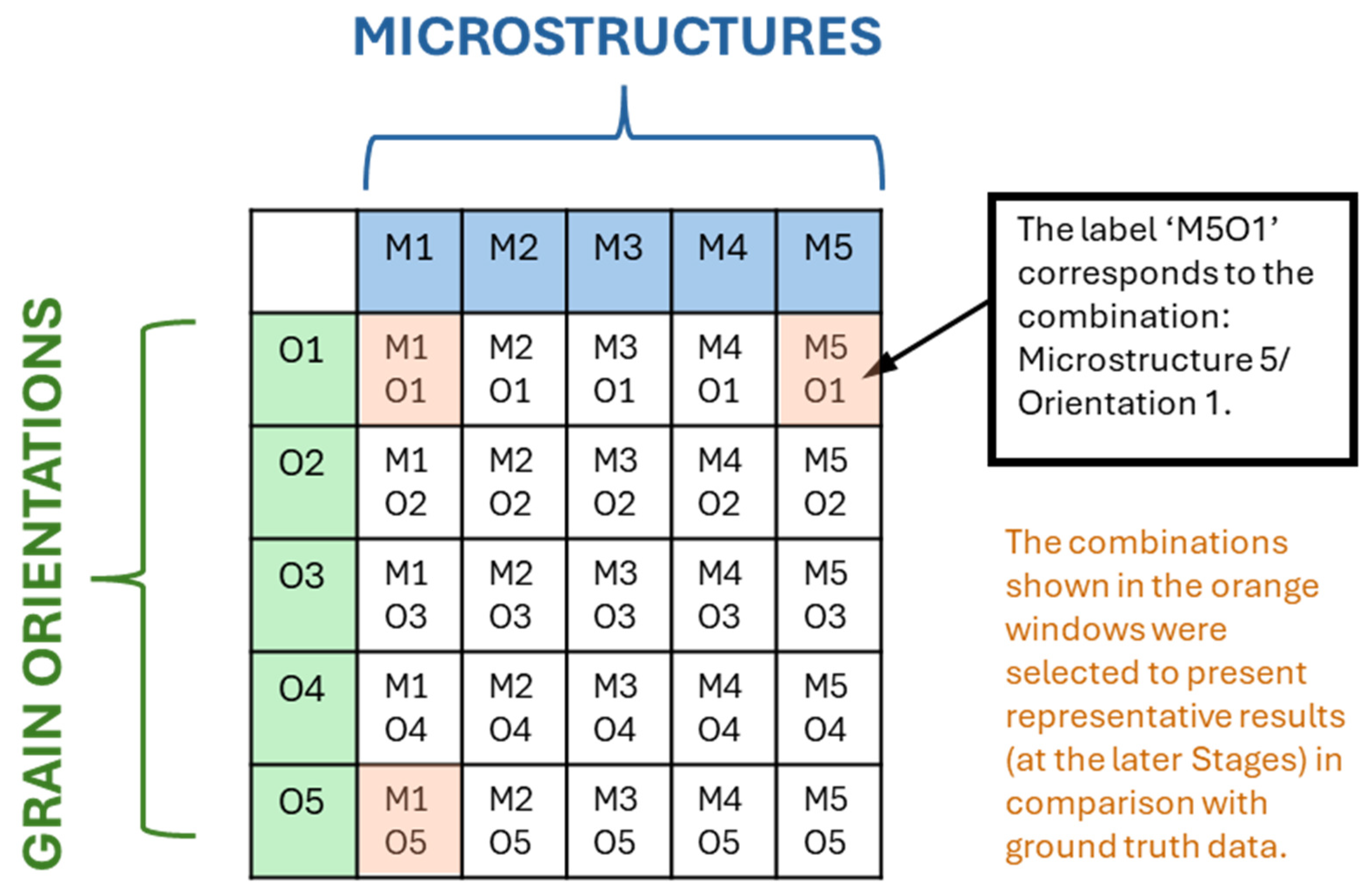
Our first challenge was to validate the CP-FFT model predictions of SSCs against the ground-truth SSCs. To accomplish this task, and with an eye to mimicking the natural variability found in microstructures, we selected 25 unique scenarios for simulations—based on 5 sets of microstructures (M1–M5) matched with 5 sets of grain orientations (O1–O5), with the (5 × 5) = 25 scenarios labelled M1O1, M2O1, M3O1, …, M5O5 as described in Figure 5. Note that details of the microstructures and grain orientations were provided in an open-access supplementary report, Ref. [22].

Figure 5. Illustration describing the labels used for the 25 different scenarios simulated. The scenarios selected to provide representative comparisons with ground-truth data during the calibration stages are also shown in orange shade.

Before an SSC could be generated for each scenario using its CP model, a set of values for the five tuneable parameters of the slip resistance Equation (7) had to be selected. We were guided by the parameter ranges reported in the literature (e.g., [14]), and the midpoints of these ranges were used to define the initial set (Table 2). Naturally, this starting set, derived somewhat arbitrarily, was not expected to be optimal; consequently, the SSCs predicted from it were not anticipated to align closely with the ground-truth curves. This was justified on the basis that these values would be subsequently refined (in Stage 3 of this work) for each scenario by comparing the DNN surrogate’s SSC predictions with the ground-truth curves. The parameter values for the dilatational plasticity model describing the elastoplastic behaviour of the pores were left unchanged, retaining the default values provided in the original publication [30]. This decision was justified by the minimal influence of pores on the overall SSCs, due to their low volume fraction in the additively manufactured AlSi10Mg material used in this study (see [22]).

Table 2. The values adopted for the adjustable parameters in the CP and dilatational plasticity models in the traditional CP-FFT simulations were based on ranges reported in the literature. Note that the value for m was not tuned in this work.

Model	a—Slip Hardening Parameter	h0 (MPa)—Overall Hardening Parameter	m—Power Law Exponent/Inverse of Rate-Sensitivity (Not Tuned in This Study)	τ0 (MPa)—Initial Value for the Slip Resistance	τb∞ or t∞ (MPa)—Saturation Value for Slip Resistance
CP model for AlSi10Mg	1	3000	20	100	200
Dilatational plasticity model for pores—values from [30]	2	1000	20	30	60

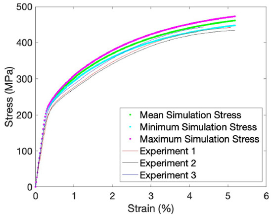
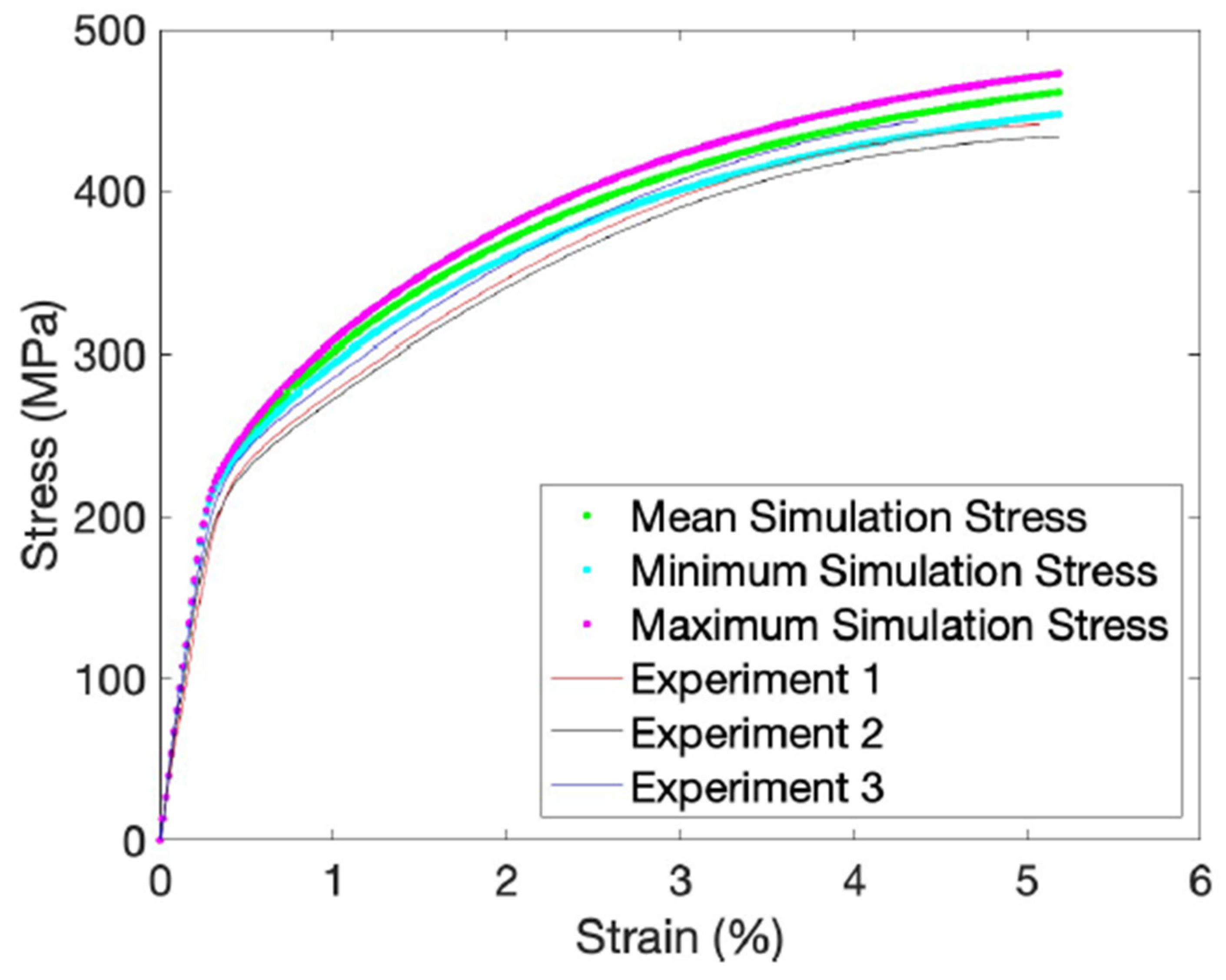
The CP-FFT physics simulation results, along with the experimental ground-truth data, are presented in Figure 6. To reduce visual clutter, the predicted stress–strain curves (SSCs) for all 25 scenarios were summarised using three representative curves: a mean curve (obtained by averaging all 25 stress values at each strain point) and curves corresponding to the minimum and maximum stress values. The predicted SSCs (using the initial set of values for the tuneable parameters) slightly overestimated the stresses relative to the experiments. Importantly, the current simulations also reproduced the experimental scatter, capturing the variability arising from different SERVE/grain orientation combinations that distinguished each scenario. This consistency with experiments further supported the validity of our model’s formulation and results.

Figure 6. A comparison between CP-FFT simulated SSCs and experimental SSCs. All three experimental ground-truth curves are shown along with the mean, minimum, and maximum SSCs generated from a total of 25 unique simulations.

3. Stage 2: DNN Surrogates and Minimum Training Data Requirements

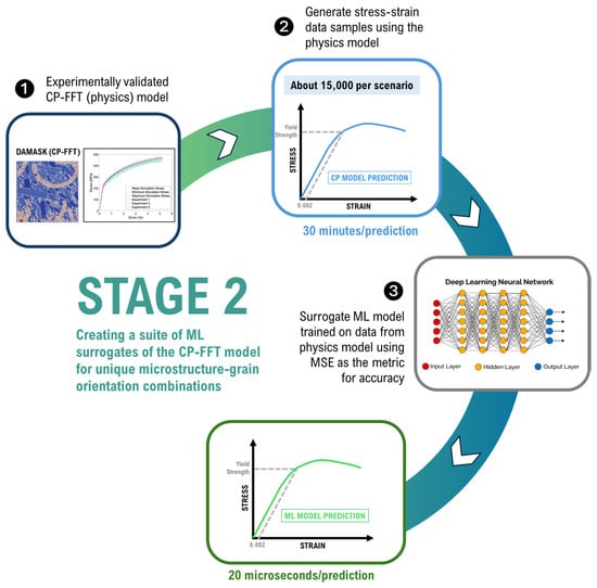
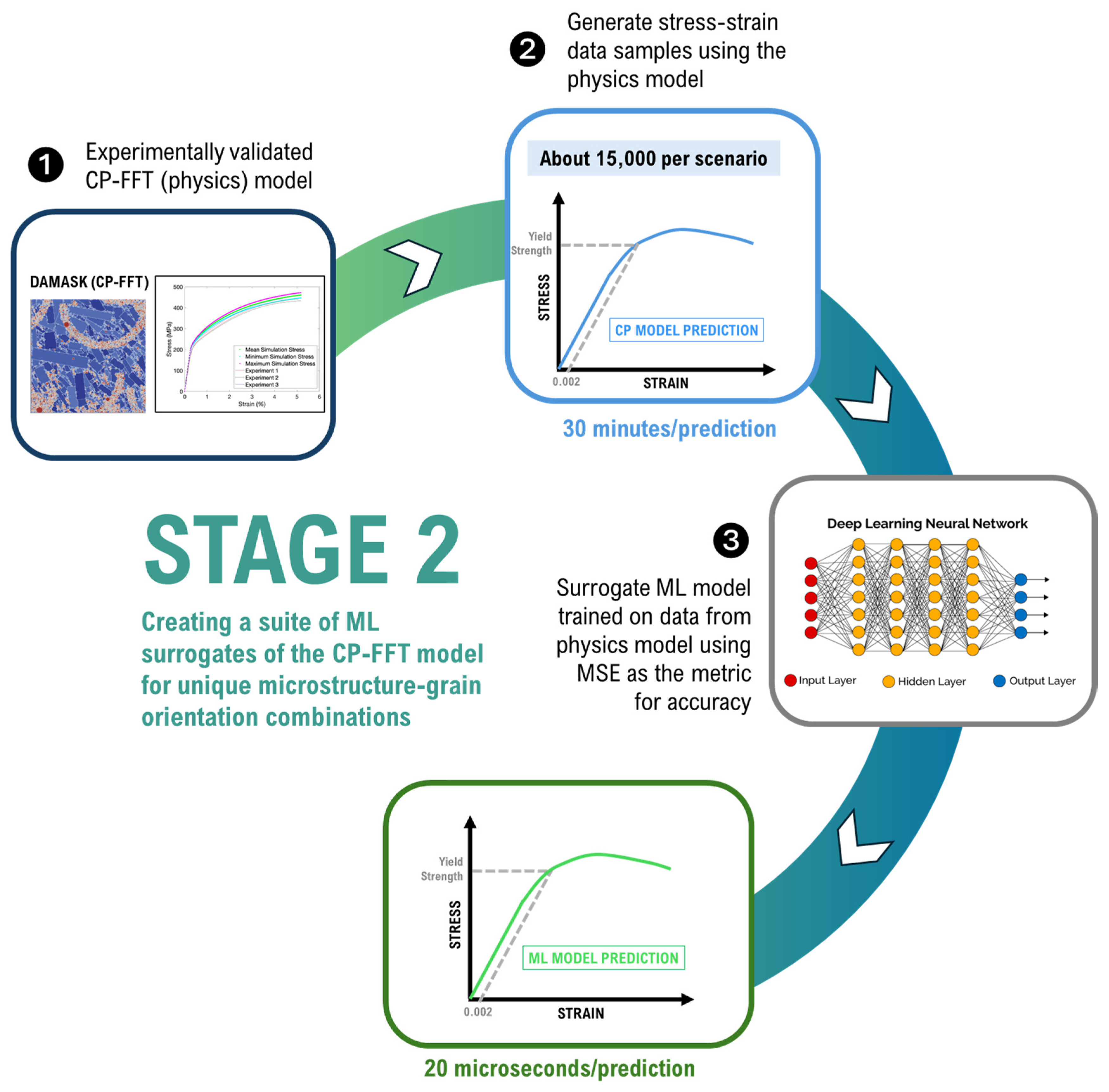
The first key task in Stage 2 was to develop DNN surrogate models for each of the 25 scenarios outlined in Figure 5. An overview of the methodology followed is provided in Figure 7 and the accompanying text below, while the detailed DNN structure, training procedures, performance indicators, and solution times are presented in [23], an open-access supplementary report. We also established the minimum number of datasets needed to train the DNNs with sufficient accuracy. This insight enables future studies to reduce the number of costly CP-FFT simulations, each of which generates a dataset that relates tuneable CP parameter values to the corresponding stress–strain response.

Figure 7. Stage 2 of the work focused on developing a suite of surrogate ML models for the experimentally validated CP-FFT model to predict the stress–strain behaviour of AM AlSi10Mg. A total of 25 surrogates were trained to represent the 25 unique scenarios = 5 microstructures × 5 sets of grain orientations.

Work in this stage focused on creating DNN surrogate models that mimicked the input-output relationships of the experimentally validated CP-FFT model developed in Stage 1. The expectation was that, once trained, the DNN could replace the physics model to rapidly generate numerous additional SSC predictions for each scenario with different parameter sets. This would enable testing a wide range of candidate parameter values in the upcoming Stage 3, which would not be feasible within a reasonable timeframe without a fast solver such as the DNN. For context, a CP-FFT simulation took, on average, 30 min to complete, whereas the corresponding DNN prediction took approximately 20 microseconds on GPU-accelerated hardware. (Note that DAMASK does not yet support GPU acceleration for CP-FFT simulations).

3.1. Generation of Datasets to Train the DNN Surrogates

The experimentally validated CP-FFT model was used to generate several new ‘CP parameter sets vs SSC’ datasets for training a separate DNN for each scenario. As ML model performance improves with larger datasets, numerous datasets were generated in an automated batch mode for each of the 25 distinct scenarios. Each prediction of the SSC featured a set of four tuneable parameters, a, h₀, τ₀, and τ_∞, from Equation (7), systematically selected from permissible ranges for each CP parameter relevant to the AlSi10Mg alloy: a $\in$ [0.5, 1.5], h₀ $\in$ [2000, 4000], τ₀ $\in$ [50, 150], and τ_∞ $\in$ [100, 300]. Guidance on the parameter bounds selected for our study was obtained from previously published works, e.g., [14]. We note that the value of the fifth tuneable parameter, m, was not varied, as this parameter is intended to capture the effect of strain rate sensitivity, whereas our experiments were all carried out at the same (i.e., constant) strain rate. The values of the adjustable parameters governing pore deformation were also left unchanged in our work, given their negligible influence on SSC shape, as our material contained only a small percentage of pores.

Eleven values were selected for each parameter range at equal intervals within the range, resulting in step sizes of 0.1, 200, 10, and 20 for a, h₀, τ₀, and τ_∞, respectively, and yielding a total of 11⁴ = 14,641 SSC predictions for each scenario. These datasets were randomly partitioned into batches of 32 (an arbitrary batch size commonly used) and split into 60%, 20%, and 20% for training, validation, and testing, respectively. This split amounted to 8784, 2928, and 2929 datasets, respectively.

The strain rate applied in the simulations was the same as that experienced during the tensile testing. Stress–strain outputs from the CP-FFT model were obtained at 1 Hz for 60 s, mirroring the experimental datalogging procedure. This typically yielded 61 data points per SSC prediction (including the initial data point at 0% strain). However, we excluded the first two data points from each SSC prediction during ML model training to reduce noise, and thus used the remaining 59 data points, which were labelled (Strain1, Stress1) … (Strain59, Stress59).

3.2. Training of the DNN Surrogates

A suite of DNN surrogates was trained, one for each scenario, comprising a unique microstructure/grain orientation combination. This allowed the potential influences of microstructure and grain orientation on SSCs to be isolated. Comprehensive details of the training procedure may be found in [23].

During training, each SSC predicted by the DNN was compared with the corresponding SSC predicted by the CP-FFT model, using the same set of CP parameters, microstructures, and grain orientations. Consequently, error metrics were obtained for the 25 different categories in the form of the coefficient of determination (R²), mean absolute error (MAE), MSE, and RMSE. However, to enable a concise tabular presentation, these 25 values were averaged over 5 grain orientations, resulting in 25/5 = 5 categories, which are effectively related to the five microstructures M1–M5. The results are presented in Table 3 row-wise for the DNNs corresponding to each microstructure as averages of metrics calculated for all 5 orientations corresponding to that microstructure. For instance, the first row contains the metrics averaged for M1O1, M1O2, M1O3, M1O4, and M1O5.

Table 3. Error metrics that compare the SSC predictions of scenario DNN surrogates with the corresponding parent SSCs generated by the CP-FFT model for each scenario. The metrics were averaged across the five grain orientations investigated for each microstructure.

DNNs Corresponding to Microstructure (Averaged over Orientations O1–O5)	R2	Mean Absolute Error (MPa)	Mean Squared Error (MPa2)	Root Mean Square Error (MPa)
M1	0.9994	0.0229	0.0009	0.0236
M2	0.9992	0.0220	0.0011	0.0264
M3	0.9994	0.0210	0.0006	0.0243
M4	0.9995	0.0179	0.0004	0.0213
M5	0.9978	0.0198	0.0022	0.0369

The results in Table 3 showed that the scenario DNNs very faithfully replicated the CP-FFT predictions, as evidenced by the consistently very high R² values and very low MAE, MSE, and RMSE values.

3.3. Finding the Minimum Number of Datasets to Train the DNN Surrogates

As noted earlier, a total of 14,641 SSC predictions from CP-FFT simulations were used to train the DNNs developed for each scenario. Generating these predictions required an equivalent number of computationally intensive CP-FFT simulations to produce the necessary parameter–SSC pairs. Although the current study adopted a conservative approach in using a large number of datasets, it was also essential to assess how DNN accuracy varied with the number of training datasets, so that we could identify the minimum number of datasets that could be used without materially compromising DNN performance. Such an analysis was motivated by the need to avoid the substantial effort and computational costs associated with performing redundant CP-FFT simulations in future investigations employing the same methodology.

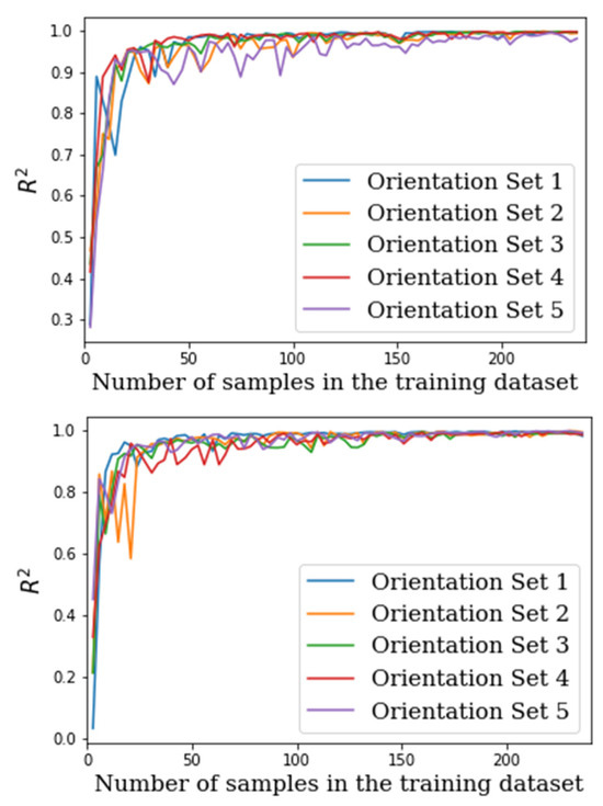
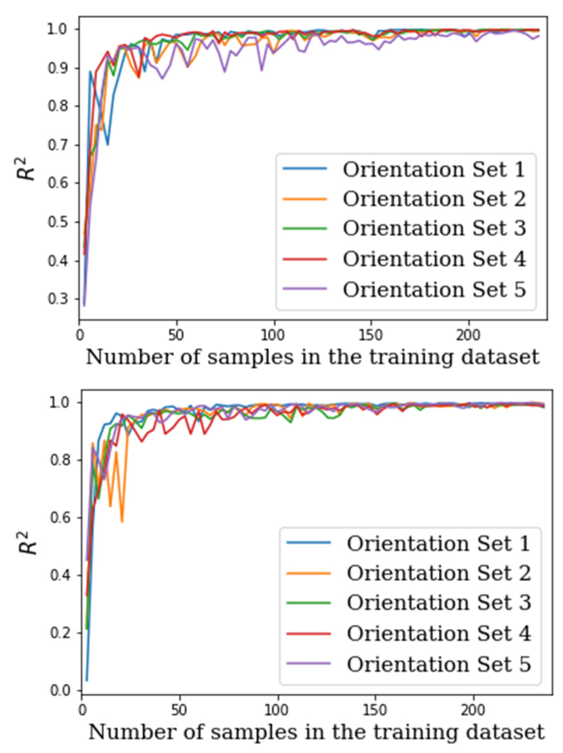
We used a trial-and-error approach to determine the minimum number of parameter-SSC datasets needed to train DNNs across all 25 scenarios. We began by using only 3 SSCs for training in each scenario, allocating 1 SSC to validation and the remaining 14,637 to testing. The number of training samples was increased by 3 at each subsequent training session, reaching 312 after 104 sessions. R² values were calculated for each training session, and the results are shown in Figure 8 for two representative cases, Microstructures M1 (left) and M5. The results for orientation sets O1–O5 within each of these microstructures are plotted separately. The R² values increased with the number of SSC samples, tending towards unity in all cases.

Figure 8. Plots of R² values obtained by comparing the surrogate predictions with corresponding CP-FFT SSCs (using the same set of CP parameters) as a function of the number of SSCs used to train the surrogates for scenarios based on microstructures M1 (left) and M5.

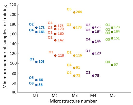
The next step was to determine the number of SSC samples beyond which the R² values showed only a marginal increase. To determine this quantity, we evaluated every tenth value (to avoid comparing adjacent values due to the oscillatory nature of the plots) until we identified the value on each plot beyond which the increase was <1%. These quantities are catalogued in Table 4 and graphically represented in Figure 9 for all 25 scenarios.

Table 4. The threshold number of SSC samples above which only marginal increases in R² were observed for each scenario. These indicated the minimum number of datasets required for training to achieve an acceptable level of accuracy for each scenario.

	< ------------------------------------------------- Microstructures ---------------------------------------------- >
Orientations	M1	M2	M3	M4	M5
O1	103	160	116	120	173
O2	173	147	75	75	164
O3	56	116	173	173	164
O4	164	176	91	144	97
O5	66	170	204	164	151

Figure 9. A plot of information tabulated in Table 4. The x-axis shows the microstructure label, while the associated grain orientation is indicated by a label beside each plotted point.

According to our criterion, the scenario requiring the most SSCs (204) for training was M3O5 (Figure 9). Therefore, we retrained all 25 DNN surrogates using 204 randomly selected SSCs and juxtaposed the R² values with those derived from the complete set of SSCs (i.e., 8784) in Table 5. Evidently, the R² values decreased only slightly as the number of training samples was reduced (i.e., from 8784 to 204), underscoring the remarkable learning capability of the DNNs. This outcome substantially reduces the computational time required to generate SSCs from the CP-FFT models in future comparable works. We speculate that this minimum number would provide useful guidance for investigating alloys whose stress–strain curves broadly resemble that of AM AlSi10Mg studied in this work.

Table 5. R² error metrics resulting from using 204 and 8784 datasets for training DNNs. The values in each row are averaged across five grain orientations associated with each microstructure.

DNNs Corresponding to Microstructure	R2 from Training with 204 Samples	R2 from Training with 8784 Samples [23]
	Averaged over Orientations O1–O5
M1	0.9853	0.9891
M2	0.9792	0.9891
M3	0.9763	0.9894
M4	0.9828	0.9898
M5	0.9851	0.9900

The SSC datasets were partitioned using train_test_split with shuffling disabled to ensure a deterministic and progressively expanding training subset. As the SSCs were generated to span the parameter space systematically, this deterministic ordering does not introduce bias in the incremental training procedure. The reported minimum dataset size should therefore be interpreted as representative for the given parameter-space sampling rather than as a statistically averaged lower bound.

4. Stage 3: Parameter Discovery

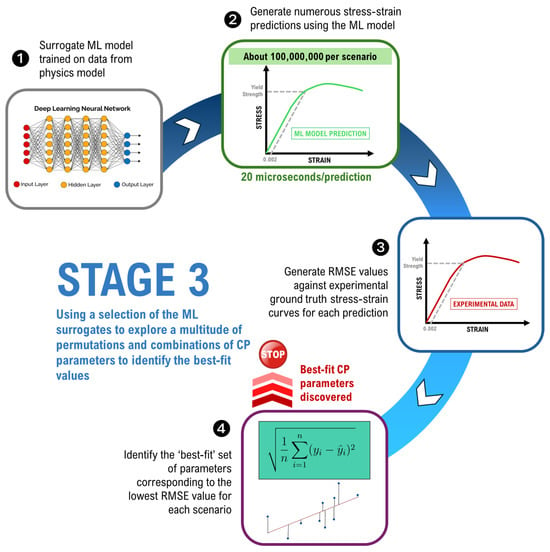
In Stage 3, we used a GSS strategy to identify the best-fit CP parameters and quantified the time savings flowing from the use of DNN surrogates in the GSS compared with the traditional trial-and-error methodology, which typically used the physics simulations (Figure 10). GSS is essentially an automated version of the traditional approach, in which different candidate model parameter sets are evaluated through trial-and-error. We investigated an extraordinarily large number of CP parameter sets using GSS, and the set yielding the best fit between the DNN-predicted and ground-truth SSCs was selected as optimal. RMSE was used as the indicator of accuracy.

Figure 10. Stage 3 of the work aimed to identify the best-fit CP model parameters using a Grid Search Scheme (GSS).

The first step was to generate an exceedingly large number of SSC predictions for each scenario using its DNN surrogate across various parameter combinations, and to calculate RMSE for each predicted curve relative to the experimental ground-truth SSCs (Figure 10). The rationale was that evaluating such a vast array of predictions, with various permutations and combinations of CP parameters, would likely yield a best-fit parameter set close to optimal. Since we used three experimental SSCs as the ground truth, three RMSE values were computed for each DNN prediction. Once all RMSE values were available for a scenario, the best-fit values were extracted for each ground-truth SSC in that scenario.

4.1. The Grid Search Scheme (GSS)

GSS systematically evaluated numerous SSC predictions from the surrogate model and, by comparing the RMSEs between the DNN-predicted SSCs and ground-truth SSCs, identified the CP parameter combination that best replicated each of the three ground-truth SSCs. The parameter set yielding the lowest RMSE value was deemed the most suitable for describing the simulated phenomenon—in our case, the stress–strain behaviour of AM AlSi10Mg, represented by the SSCs. The expectation was that by exhaustively exploring a vast number of permutations and combinations, a sufficiently expansive parameter space could be searched to identify the best-fitting set.

While grid search is straightforward to implement, it can be extremely time-consuming and computationally expensive, especially when the number of parameters is large. This method is also less scalable than other optimisation techniques due to the exponential growth in the number of combinations as the number of parameters increases. Additionally, there is no guarantee that the optimal parameter set will be identified, even after a comprehensive search, because some combinations may still be overlooked, including the optimal set. Furthermore, if the optimal parameter set lies outside the defined search space, the GSS cannot identify it because it is restricted to evaluating parameters within the specified grid. More details on this method, sometimes used for optimising hyperparameters in ML, may be found elsewhere, e.g., Refs. [31,32].

4.2. Implementation of GSS

Our GSS space covered 101 values for each of the four tuneable CP parameters a, h₀, τ₀, and τ_∞ (Section 2.2.2) within their specified intervals: a $\in$ [0.5, 1.5], h₀ $\in$ [2000, 4000], τ₀ $\in$ [50, 150], and τ_∞ $\in$ [100, 300]. This resulted in 101⁴ = 104,060,401 combinations of these parameters for each scenario outlined in Section 2.2.2. The GSS algorithm leverages a four-loop structure with a complexity of O(n⁴), viz., n = 101 in our case—to handle the extensive parameter space efficiently, thereby avoiding memory overload. This approach was necessary because generating all 104,060,401 combinations simultaneously and predicting sequentially resulted in memory overflow. Despite this added computational layer, the DNN surrogates were remarkably fast, delivering predictions at a fraction of the time required by the original CP-FFT model.

Since analysing all 25 scenarios will be onerous, given the large number of parameter combinations to be considered for each scenario, we focused our analysis on three representative scenarios: M1O1, M1O5, and M5O1 (Figure 5). The rationale was that comparing the results of M1O1 with M1O5 would reveal the impact of varying orientation, while comparing the results of M1O1 with M5O1 would demonstrate the effect of altering the microstructure.

We used DNNs trained with the full 8784 datasets for the GSS. After normalising the parameter values of our GSS space using the same min-max scaling technique employed during surrogate training [23], we predicted the associated SSC for each of the 101,060,401 parameter combinations using the trained models. Since the model outputs were normalised using score normalisation at the training stage, the predictions were subsequently denormalised using the same score normalisation parameters (mean and standard deviation) to revert them to their original scales.

To enable a fair comparison between the predicted SSCs and the ground-truth SSCs labelled GT1, GT2, and GT3), the ground-truth SSCs, which originally consisted of 264, 232, and 227 points, respectively, were interpolated to match the 59 points of the DNN’s output [23]. This interpolation was performed using scipy.interpolate.CubicSpline from SciPy python library [33,34] over a fixed strain range of [0, 5] with 61 equally spaced points. (Note: We dropped the first two strain points as discussed in [23]. We identified the optimal parameter sets by evaluating each predicted SSC against the interpolated ground-truth SSCs, yielding three fitness values for each prediction.

The fitness comparison was based on RMSE calculated using:

$$RMSE= \sqrt{{\displaystyle \frac{\sum {\left(y_p-y_{gt}\right)}^2}{N}}}$$

(11)

where y_p = predicted stress value for any given strain value, y_gt = corresponding ground-truth stress value and N = number of observations (59 for each SSC as described in [23].

The parameter set yielding the minimum RMSE value was identified separately for each ground-truth SSC (GT1, GT2, and GT3), resulting in three distinct optimal parameter sets for every SSC prediction.

Results from the GSS are presented in Section 5 below.

5. Results and Discussion

5.1. Best-Fit Values for the Tuneable Parameters and Computation Times

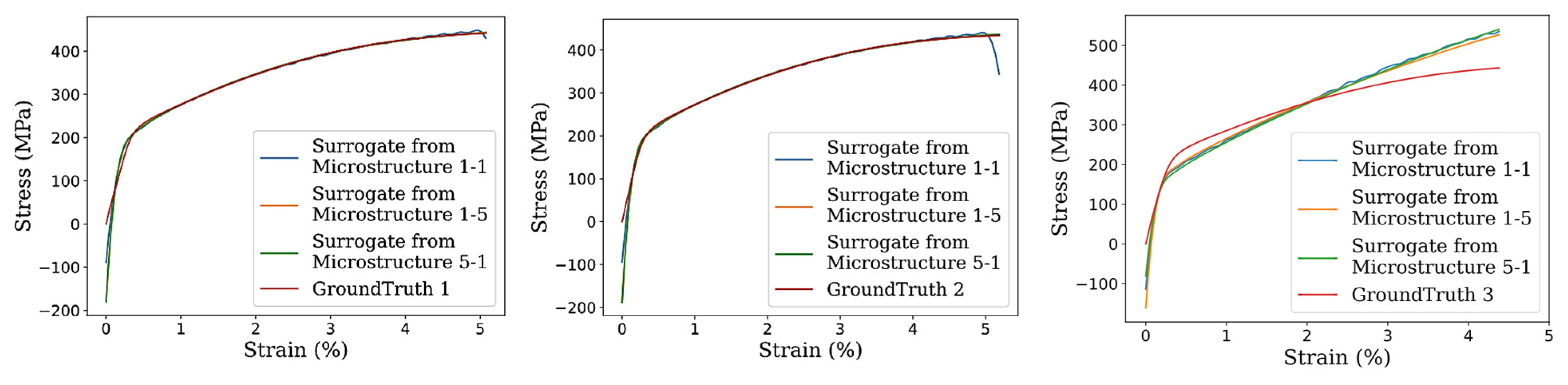
As discussed previously, the GSS approach is designed to provide only the best-fit parameter values that it finds (Table 6) based on the grid values investigated rather than optimum parameter values. The values extracted by GSS in the current study yielded reasonably small RMSEs between scenario DNN predictions for the three models investigated (M101, M105, and M501) and the ground-truths GT1, GT2, and GT3. The good accuracies are confirmed by the reasonably good fits obtained from generating SSCs using these values via the CP-FFT simulations (Figure 11). The worst fit was observed for GT3, and was accompanied by the substantially higher associated RMSE (Table 6). It is worth noting that the GT3 sample failed relatively early during tensile testing, i.e., before achieving 4.5% strain (see shorter experimental plot on Figure 6). This may indicate that the sample’s mechanical properties were affected by microstructural defects (e.g., porosity). Therefore, we may have to treat GT3 as an anomaly.

Table 6. Best-fit values for CP parameters extracted by GSS for each ground-truth (GT) per scenario. Results for only 9 representative scenarios (out of 25) are given here. The computation times were estimated by dividing the total time taken to complete the simulations for a given scenario for all three GTs by 3.

	GT1			GT2			GT3
Scenario Model →	M101	M105	M501	M101	M105	M501	M101	M105	M501
a [0.5, 1.5]	0.67	0.66	0.63	0.63	0.63	0.66	0.67	0.7	0.59
h [2000, 4000] MPa	2140	2160	2100	2000	2060	2080	2000	2000	2000
τ0 [50, 150] MPa	89	90	89	88	89	88	77	80	73
τ∞ [100, 300] MPa	186	182	184	182	178	182	300	300	300
RMSE (MPa)	4.4437	4.4779	4.398	2.3024	2.3057	2.1739	90.446	90.467	90.103
Computation Time (s) est.	33,122.46	33,035.29	33,042.89	33,122.46	33,035.29	33,042.89	33,122.46	33,035.29	33,042.89

Figure 11. SSCs predicted using best-fit-parameter values returned by GSS for the three ground-truths—(left) GT1, (middle) GT2, and (right)—GT3.

Notably, the best-fit values identified for the tuneable CP parameters a, h, τ₀, and τ_∞ were remarkably consistent across the scenarios for each GT, with only minor exceptions. Such regularity in parameter values is unsurprising, given that the microstructures and grain orientations constituting each scenario were obtained from the same location on the gauge length. Additionally, the relatively small scatter among the GT curves (Figure 6) resulted in parameter values that were similar across GTs, except for GT3, which is regarded as an outlier. Moreover, because a vast parameter space (104,060,401 sets) was investigated for each of the 25 scenarios, the value extracted for each parameter is likely located close to the parameter’s optimal value for that scenario.

The computation time to test all candidate sets in GSS and determine the best-fit sets was approximately 33,000 s (about 9.2 h) per scenario.

The results in Table 6 shows that the extracted parameter values do not lie near the mid-range of those typically reported for AlSi10Mg alloys, particularly for parameters a and h. This deviation accounts for the discrepancy observed in Figure 6 between the ground-truth SSCs and their CP-FFT-simulated counterparts, for which midpoint parameter values were assumed.

Our results are broadly consistent with values reported in the literature for additively manufactured AlSi10Mg alloys (Table 7), although some differences are evident. These variances may stem from two factors: (1) the substantially larger parameter space explored in the present work to identify best-fit values, and (2) inherent variations in AM microstructures arising from differences in processing conditions (for the same alloy).

Table 7. Values for CP parameters reported by others for the AM AlSi10Mg alloy.

Parameter	Zhang and Andra [14]	Bisht et al. [35]
a [0.5, 1.5]	1.2	1.0
h [2000, 4000] MPa	2000	1400
τ0 [50, 150] MPa	112	100
τ∞ [100, 300] MPa	187	190

5.2. Computational Time Savings Resulting from the Use of DNNs

Details of the hardware used in our study are provided here first to contextualise the computation times reported below. The hardware configurations we used are typical of those used by physics modellers and data scientists. Note that the popular CP-FFT simulation code used here, DAMASK, does not yet support GPU acceleration (although some researchers have accelerated certain parts of the calculations using custom GPU codes).

For CP-FFT simulations: Linux machine without a GPU (16 threads in a dual AMD EPYC 7543 32-Core Processors (2.8 GHz) with 512 GB RAM).

For all ML-related work: Linux machine equipped with 24 CPU Cores with 20 GB RAM and an NVIDIA Tesla V100-32 GB GPU (NVIDIA, Santa Clara, CA, USA).

Time savings ts_scenario achieved per scenario by our methodology over the conventional trial-and-error approach may be estimated as:

ts_scenario = t_conventional − t_datasets − t_{DNN training} − t_GSS,

(12)

where t_conventional = estimated time taken to generate SSC predictions for all the candidate sets used in GSS for a given scenario through a conventional approach using CP-FFT simulations, t_datasets = time taken to generate datasets to train a DNN for a given scenario, t_{DNN training} = time taken to train a DNN for a scenario, and t_GSS = time taken to generate SSC predictions for all the candidate sets used in GSS for a given scenario and finding the best-fitting set.

The value for t_conventional may be estimated by multiplying the number of candidate sets tested in GSS for each scenario by the time required to complete a CP-FFT simulation (30 min = 1800 s), since one physics simulation per set is required to generate the resulting SSC. Since we tested 104,060,401 sets, the nominal time that one would have spent performing physics simulations for the traditional trial-and-error procedure:

t_conventional = 104,060,401 × 1800 = 181,908,720,000 s

(13)

The time required to generate 8784 datasets for training each DNN (since each dataset requires a CP-FFT simulation to be carried out):

t_datasets = 8784 × 1800 + 2 s = 15,811,204 s,

(14)

Including 2 s consumed for reading the custom-formatted CP-FFT output, converting them into input and output arrays, and then dividing them into training, validation, and test datasets. Note that, although the computation time of 15,811,204 s above corresponds to 183 days, we ran several simulations in parallel. This enabled us to obtain the required datasets within a month.

The time taken for training of each DNN surrogate using 8784 datasets:

t_{DNN training} = 177 s

(15)

Note that if we had used the minimum number, 204, required for training (Section 3.3), the time required for this task would have been accordingly reduced.

The time required to perform the GSS computations for a scenario:

t_GSS = 33,000 s

(16)

Therefore, computation time saved per scenario (as per Equation (11)):

ts_scenario = 181,908,720,000 − 15,811,204 − 177 − 33,000 = 181,892,875,621 s = 5767 years

(17)

This yields a saving of 25 × 5767 = 144,175 years across all 25 scenarios. This represents an incredible reduction in computational cost and underscores the effectiveness of our methodology, which enabled exploration of a vast parameter space that would otherwise have been infeasible.

6. Conclusions

Phenomenological CP models provide a robust framework for linking microstructural features to macroscopic mechanical behaviour within ICME workflows. However, the substantial computational cost of physics-based simulations, together with the demanding nature of parameter calibration, has limited their widespread use in practical and industrial applications. There is therefore a strong need for approaches that accelerate these simulations and streamline parameter identification, thereby broadening the applicability of CP models in simulation-driven materials engineering and optimisation. In this work, we presented an efficient framework that combined ML surrogates of physics-based CP models with an automated grid search strategy to evaluate an unprecedented number of CP parameter sets and identify the best-performing configuration.

DNN surrogate models were trained on CP-FFT simulations to enable near-instantaneous prediction of SSCs. Leveraging the high computational speed of DNNs, we performed an exhaustive exploration of a parameter space comprising 104,060,401 candidate sets to identify the best-fit values for the phenomenological CP model. Parameters for 25 different experimentally generated scenarios, comprising 5 microstructures × 5 sets of grain orientations, were obtained. Given the scale of these searches, which covered a vast parameter space, the extracted parameters may be considered close to optimal. A grid-search strategy was employed, effectively automating the conventional trial-and-error calibration process. Additionally, we identified the minimum number of CP-FFT simulations (approximately 200) required to train a DNN with satisfactory accuracy, thereby enabling researchers to avoid redundant, computationally expensive simulations in future works. Furthermore, we quantified the computational savings of the proposed methodology relative to the traditional approach, demonstrating that the conventional approach could not have handled the scale of our parameter space. The computation time associated with the calibration procedure can be shortened by an incomprehensible several thousand years using the proposed framework, and when each CP-FFT simulation is replaced by a DNN prediction, the per-simulation cost is reduced by roughly 30 min. The times required for dataset generation, DNN training, and grid-search evaluation were also reported.

The advantages of the rapid calibration framework are particularly significant for AM materials, where spatially varying properties necessitate repeated parameter tuning to construct accurate property maps. The methodology was demonstrated using an L-PBF AM AlSi10Mg alloy.

We anticipate that this study will contribute to the broader adoption of CP modelling across a wide range of materials systems, with particular relevance to AM alloys. The proposed framework may also be used outside the current domain to calibrate various phenomenological models.

In future work, the authors will investigate the relative performances of optimisation algorithms compared with the GSS (in terms of accuracy and efficiency) for calibrating CP models.

References

- Kapoor, K.; Ravi, P.; Noraas, R.; Park, J.-S.; Venkatesh, V.; Sangid, M.D. Modeling Ti–6Al–4V using crystal plasticity, calibrated with multi-scale experiments, to understand the effect of the orientation and morphology of the α and β phases on time dependent cyclic loading. J. Mech. Phys. Solids 2021, 146, 104192. [Google Scholar] [CrossRef] [Scilit]
- Yaghoobi, M.; Chen, Z.; Sundararaghavan, V.; Daly, S.; Allison, J.E. Crystal Plasticity Finite Element Modeling of Extension Twinning in WE43 Mg Alloys: Calibration and Validation. Integr. Mater. Manuf. Innov. 2021, 10, 488–507. [Google Scholar] [CrossRef] [Scilit]
- Ali, U.; Muhammad, W.; Brahme, A.; Skiba, O.; Inal, K. Application of artificial neural networks in micromechanics for polycrystalline metals. Int. J. Plast. 2019, 120, 205–219. [Google Scholar] [CrossRef] [Scilit]
- Bonatti, C.; Berisha, B.; Mohr, D. From CP-FFT to CP-RNN: Recurrent neural network surrogate model of crystal plasticity. Int. J. Plast. 2022, 158, 103430. [Google Scholar] [CrossRef] [Scilit]
- Dai, W.; Wang, H.; Guan, Q.; Li, D.; Peng, Y.; Tomé, C.N. Studying the micromechanical behaviors of a polycrystalline metal by artificial neural networks. Acta Mater. 2021, 214, 117006. [Google Scholar] [CrossRef] [Scilit]
- Martinitz, L.; Hartmann, C. An artificial neural network approach on crystal plasticity for material modelling in macroscopic simulations. IOP Conference Series. Mater. Sci. Eng. 2023, 1284, 012052. [Google Scholar] [CrossRef] [Scilit]
- Montes de Oca Zapiain, D.; Lim, H.; Park, T.; Pourboghrat, F. Predicting plastic anisotropy using crystal plasticity and Bayesian neural network surrogate models. Mater. Sci. Eng. A 2022, 833, 142472. [Google Scholar] [CrossRef] [Scilit]
- Nascimento, A.; Roongta, S.; Diehl, M.; Beyerlein, I.J. A machine learning model to predict yield surfaces from crystal plasticity simulations. Int. J. Plast. 2023, 161, 103507. [Google Scholar] [CrossRef] [Scilit]
- Pandey, A.; Pokharel, R. Machine learning based surrogate modeling approach for mapping crystal deformation in three dimensions. Scr. Mater. 2021, 193, 1–5. [Google Scholar] [CrossRef] [Scilit]
- Pokharel, R.; Pandey, A.; Scheinker, A. Physics-Informed Data-Driven Surrogate Modeling for Full-Field 3D Microstructure and Micromechanical Field Evolution of Polycrystalline Materials. JOM 2021, 73, 3371–3382. [Google Scholar] [CrossRef] [Scilit]
- Saidi, P.; Pirgazi, H.; Sanjari, M.; Tamimi, S.; Mohammadi, M.; Béland, L.K.; Daymond, M.R.; Tamblyn, I. Deep learning and crystal plasticity: A preconditioning approach for accurate orientation evolution prediction. Comput. Methods Appl. Mech. Eng. 2022, 389, 114392. [Google Scholar] [CrossRef] [Scilit]
- Yang, Z.; Papanikolaou, S.; Reid, A.C.E.; Liao, W.-K.; Choudhary, A.N.; Campbell, C.; Agrawal, A. Learning to Predict Crystal Plasticity at the Nanoscale: Deep Residual Networks and Size Effects in Uniaxial Compression Discrete Dislocation Simulations. Sci. Rep. 2020, 10, 8262. [Google Scholar] [CrossRef] [Scilit]
- Yuan, M.; Paradiso, S.; Meredig, B.; Niezgoda, S.R. Machine Learning–Based Reduce Order Crystal Plasticity Modeling for ICME Applications. Integr. Mater. Manuf. Innov. 2018, 7, 214–230. [Google Scholar] [CrossRef] [Scilit]
- Zhang, X.X.; Andrä, H. Crystal plasticity simulation of the macroscale and microscale stress–strain relations of additively manufactured AlSi10Mg alloy. Comput. Mater. Sci. 2021, 200, 110832. [Google Scholar] [CrossRef] [Scilit]
- Charmi, A.; Falkenberg, R.; Ávila, L.; Mohr, G.; Sommer, K.; Ulbricht, A.; Sprengel, M.; Neumann, R.S.; Skrotzki, B.; Evans, A. Mechanical anisotropy of additively manufactured stainless steel 316L: An experimental and numerical study. Mater. Sci. Eng. A 2021, 799, 140154. [Google Scholar] [CrossRef] [Scilit]
- Hansen, C.K.; Whelan, G.F.; Hochhalter, J.D. Interpretable machine learning for microstructure-dependent models of fatigue indicator parameters. Int. J. Fatigue 2024, 178, 108019. [Google Scholar] [CrossRef] [Scilit]
- Sadeghpour, E.; Nonn, A. Data-driven models for structure-property prediction in additively manufactured steels. Comput. Mater. Sci. 2022, 215, 111782. [Google Scholar] [CrossRef] [Scilit]
- Saunders, R.N.; Teferra, K.; Elwany, A.; Michopoulos, J.G.; Lagoudas, D. Metal AM process-structure-property relational linkages using Gaussian process surrogates. Addit. Manuf. 2023, 62, 103398. [Google Scholar] [CrossRef] [Scilit]
- Shen, T.; Li, B. An integrated computation framework for predicting mechanical performance of single-phase alloys manufactured using laser powder bed fusion: A case study of CoCrFeMnNi high-entropy alloy. Mater. Today Commun. 2024, 39, 109180. [Google Scholar] [CrossRef] [Scilit]
- Tu, Y.; Liu, Z.; Carneiro, L.; Ryan, C.M.; Parnell, A.C.; Leen, S.B.; Harrison, N.M. Towards an instant structure-property prediction quality control tool for additive manufactured steel using a crystal plasticity trained deep learning surrogate. Mater. Des. 2022, 213, 110345. [Google Scholar] [CrossRef] [Scilit]
- Bishara, D.; Li, S. A machine-learning aided multiscale homogenization model for crystal plasticity: Application for face-centered cubic single crystals. Comput. Mech. 2023, 72, 77–93. [Google Scholar] [CrossRef] [Scilit]
- Gunasegaram, D.R. Appendix A—Supplementary Material for Stage 1 Crystal Plasticity Model; CSIRO: Melbourne, Australia, 2025; p. 7. Available online: https://publications.csiro.au/publications/publication/PIcsiro:EP2025-3099 (accessed on 2 March 2026).
- Samadiani, N. Appendix B—Supplementary Material for Stage 3 Deep Neural Networks; CSIRO: Melbourne, Australia, 2025; p. 7. Available online: https://publications.csiro.au/publications/publication/PIcsiro:EP2025-3101 (accessed on 2 March 2026).
- Roters, F.; Diehl, M.; Shanthraj, P.; Eisenlohr, P.; Reuber, C.; Wong, S.; Maiti, T.; Ebrahimi, A.; Hochrainer, T.; Fabritius, H.-O.; et al. DAMASK—The Düsseldorf Advanced Material Simulation Kit for modeling multi-physics crystal plasticity, thermal, and damage phenomena from the single crystal up to the component scale. Comput. Mater. Sci. 2019, 158, 420–478. [Google Scholar] [CrossRef] [Scilit]
- Roters, F.; Eisenlohr, P.; Bieler, T.R.; Raabe, D. Introduction to Crystalline Anisotropy and the Crystal Plasticity Finite Element Method. In Crystal Plasticity Finite Element Methods; Wiley: Hoboken, NJ, USA, 2010; pp. 1–9. [Google Scholar]
- Roters, F.; Eisenlohr, P.; Hantcherli, L.; Tjahjanto, D.; Bieler, T.; Raabe, D. Overview of constitutive laws, kinematics, homogenization and multiscale methods in crystal plasticity finite-element modeling: Theory, experiments, applications. Acta Mater. 2010, 58, 1152–1211. [Google Scholar] [CrossRef] [Scilit]
- Liu, J.; Xiong, W.; Behera, A.; Thompson, S.; To, A.C. Mean-field polycrystal plasticity modeling with grain size and shape effects for laser additive manufactured FCC metals. Int. J. Solids Struct. 2017, 112, 35–42. [Google Scholar] [CrossRef] [Scilit]
- Roters, F.; Eisenlohr, P.; Bieler, T.R.; Raabe, D. Constitutive Models. In Crystal Plasticity Finite Element Methods; Wiley: Hoboken, NJ, USA, 2010; pp. 47–91. [Google Scholar]
- Hutchinson, J.W.; Hill, R. Bounds and self-consistent estimates for creep of polycrystalline materials. Proc. R. Soc. Lond. A Math. Phys. Sci. 1976, 348, 101–127. [Google Scholar] [CrossRef] [Scilit]
- Maiti, T.; Eisenlohr, P. Fourier-based spectral method solution to finite strain crystal plasticity with free surfaces. Scr. Mater. 2018, 145, 37–40. [Google Scholar] [CrossRef] [Scilit]
- So, A.; Joseph, T.V.; John, R.T.; Worsley, A.; Asare, S. The Data Science Workshop: Learn How You Can Build Machine Learning Models and Create Your Own Real-World Data Science Projects, 2nd ed.; Packt Publishing: Birmingham, UK, 2020. [Google Scholar]
- Stripling, G.; Abel, M. Low-Code AI; O’Reilly Media: Sebastopol, CA, USA, 2023. [Google Scholar]
- Press, W.H.; Teukolsky, S.A.; Vetterling, W.T.; Flannery, B.P. Numerical Recipes 3rd Edition: The Art of Scientific Computing; Cambridge University Press: Cambridge, UK, 2007. [Google Scholar]
- Virtanen, P.; Gommers, R.; Oliphant, T.E.; Haberland, M.; Reddy, T.; Cournapeau, D.; Burovski, E.; Peterson, P.; Weckesser, W.; Bright, J.; et al. Author Correction: SciPy 1.0: Fundamental algorithms for scientific computing in Python. Nat. Methods 2020, 17, 352. [Google Scholar] [CrossRef] [Scilit]
- Bisht, M.S.; Gaur, V.; Singh, I.V. A Study of Strengthening and Hardening Micro-mechanisms in Additively Built AlSi10Mg Using Crystal Plasticity Simulations. Met. Mater. Int. 2025, 31, 2855–2874. [Google Scholar] [CrossRef] [Scilit]
Disclaimer/Publisher’s Note: The statements, opinions and data contained in all publications are solely those of the individual author(s) and contributor(s) and not of MDPI and/or the editor(s). MDPI and/or the editor(s) disclaim responsibility for any injury to people or property resulting from any ideas, methods, instructions or products referred to in the content. |
© 2026 by the authors. Licensee MDPI, Basel, Switzerland. This article is an open access article distributed under the terms and conditions of the Creative Commons Attribution (CC BY) license.