


Abstract
Research on eco-friendly and energy-efficient machining processes has gained significant importance within the domain of sustainable production. This study is focused on enhancing the energy performance and sustainability of the milling process. Four machine learning (ML) models, namely, multiple linear regression (MLR), support vector regression (SVR), Gaussian process regression (GPR), and adaptive network-based fuzzy inference system (ANFIS), were proposed to estimate specific energy consumption (SEC) in the milling of Ti6-Al4-V under two eco-benign cooling conditions: cryogenic and minimum quantity lubrication (MQL). Several statistical metrics, including normalized mean absolute error (nMAE), mean absolute percentage error (MAPE), normalized root mean square error (nRMSE), maximum absolute percentage error (maxAPE), coefficient of determination (R2), and Willmott’s index of agreement (IA), were employed to validate the performances of the ML models. A high level of agreement between the predicted and experimental SEC data for both the training and test datasets supports the reliability of the proposed ML models. Although the MLR model performed well, the results revealed that the other ML models demonstrated better overall performance. According to the statistical metrics, the models’ predictive performance improved in the following sequence: MLR, SVR, GPR, and finally ANFIS, which demonstrated the highest predictive capability.
1. Introduction
In the current industrial scenario, one of the most challenging problems is sustainable production. In metal cutting processes, cutting fluids have historically been utilized to improve machining process performances, such as machinability, productivity, and cost. However, conventional (flood) cooling remains widely employed in machining, particularly for difficult-to-cut materials [1]. Difficult-to-cut materials, such as Ti-based alloys, Ni-based alloys, high-strength steels, and metal matrix composites, are increasingly employed in many industries because of their specific physical properties. Nevertheless, the high operational performance of these materials negatively influences machinability. In particular, low thermal conductivity and a strong work-hardening tendency result in high cutting forces and temperatures, which accelerate tool wear and may compromise surface integrity. These processes also require greater power to remove a given volume of material. Hence, new cooling alternatives, such as cryogenic cooling, minimum quantity lubrication (MQL), cryoMQL, etc., have been developed in order to improve the machinability of difficult-to-cut materials and as a result of the growing attention given to eco-friendly machining requirements. The electrical and embodied energy of resources are consumed during machining processes, which transform raw materials into final products. Thus, the energy efficiency has also been found to be crucial in the transition towards sustainable manufacturing. Owing to rising energy consumption and limited resources, the metal cutting industry faces increasingly stringent ecological and energy-related requirements [2]. As a major component of industrial operations, the metal processing sector consumes a significant amount of energy, accounting for nearly 40% of global industrial energy use. Additionally, carbon dioxide emissions in this sector have risen by 50% over the past two decades [3]. Most energy consumption in the metal cutting industry is attributed to machine tools, which are the main components of production systems [4]. These machine tools generally exhibit low energy efficiency, with less than 15% of their total energy consumption being used for the actual material removal process [5]. Energy standards, regulations, and the broader pursuit of sustainable production therefore demand continual research and energy optimization of the metal cutting processes [6]. Further incentives, such as subsidies and regulatory measures issued by international and national institutions, continue to drive improvements in the energy efficiency of machine tools.
Machine learning (ML) models have been broadly used in the prediction of different machining responses, such as cutting forces, surface quality, tool life, cutting temperature, and others. Numerous investigations on the prediction of machine tool energy consumption have also been carried out. Shin et al. [7] proposed a holonic-based mechanism for self-learning factories using a hybrid learning approach. A prototype system was implemented for milling processes to generate energy predictive models and optimize machine tool selection. Results showed an energy consumption reduction of 9.7% compared to the highest energy-consuming machine tool. Study [8] proposed a deep learning-based approach for predicting energy consumption of machine tools. Experiments on a milling machine and a grinding machine demonstrated substantial improvements in prediction accuracy compared to other studies. Cao et al. [9] developed a milling energy prediction method based on program parsing and a parallel neural network. Experiments showed prediction errors of 0.85% for total program energy and within 5% per line of instruction, with efficiency improved by nearly 50% compared to existing methods. A hybrid approach combining ML and process mechanics to predict specific cutting energy is presented in [10]. The method was validated in the milling of H13 tool steel and Inconel 718. The developed method shows significantly higher accuracy than analytical models. Zhang et al. [11] presented an energy consumption prediction method based on long short-term memory neural networks optimized by an improved particle swarm algorithm with dynamic inertia weights. Compared to other optimization methods, over 30% improvement in mean absolute and mean errors was achieved, demonstrating enhanced prediction accuracy and efficiency. An evaluation of the impact of different eco-friendly cooling techniques on carbon emissions during machining of Monel 400 alloy was presented in [12]. ML models, including decision trees, naive Bayes, random forests, and support vector machines, were used for sustainability assessment. The support vector machine achieved nearly 100% accuracy in predicting discretized carbon emission levels. Sealy et al. [13] investigated power and energy consumption in hard milling of AISI H13 tool steel at machine, spindle, and process levels, focusing on specific cutting energy. A regression model was developed to accurately predict cutting-specific energy. Brillinger et al. [14] investigated ML algorithms, such as decision tree, random forest, and boosted random forests, to predict the energy demand of CNC machining strategies. Random forest achieved the most accurate predictions, eliminating the need for dedicated experiments. Lu et al. [15] proposed a multi-pass parametric optimization method using deep reinforcement learning to improve energy efficiency. The results confirmed the effectiveness of the proposed approach in achieving energy-efficient and deformation-compliant machining. ML models applied to improve energy efficiency in 5-axis milling under various machining parameters and toolpath strategies were presented in [16]. Decision tree and random forest models outperformed linear, lasso, and ridge regression. Study [17] presented an intelligent energy monitoring method using a 1-dimensional convolutional neural network (1D-CNN) to determine machine operation status from energy consumption data. The results demonstrated that 1D-CNN outperforms deep learning and ML algorithms in analyzing time-series energy data for monitoring purposes. Awan et al. [18] developed a methodology to predict specific energy consumption in cut-off grinding using supervised machine learning. Among Gaussian process regression, regression trees, and artificial neural networks, Gaussian process regression showed the best performance with minimal validation errors. Yurtkuran et al. [19] applied ML models, such as linear regression, multilayer perceptron, gradient boosting regression, and adaboost regression, to predict power consumption during milling of PH13-8Mo stainless steel under various cutting environments, including dry, MQL, nano-graphene + MQL, nano-hBN + MQL, cryo, and cryo + MQL. The developed ML models accurately confirm the relationship between cutting parameters and power consumption. Random forest regressor was employed to predict energy consumption, productivity, and surface roughness in CNC face milling of AISI-1045 steel [20]. The results demonstrated that the proposed model can serve as a reliable prediction tool for machining processes with minimal feature selection. ML algorithms, including K-nearest neighbor, Gaussian regression, decision tree, and logistic regression, were evaluated in order to predict energy consumption in CNC machining of Inconel 718 under MQL and nanofluid-based MQL cutting environment [21]. The decision tree model achieved the highest prediction accuracy. Korkmaz et al. [22] investigated the reduction of specific cutting energy in sustainable machining of Inconel 601 using various cooling methods, including dry, MQL, nano-MQL, cryogenic, and hybrid cryo-nano-MQL. Among multiple linear regression, lasso regression, Bayesian ridge regression, and voting regressor, the Bayesian model achieved the lowest prediction error. An intelligent monitoring system for ultra-precision CNC machine tools using power consumption data instead of retrofitted sensors was presented in [23]. A G-code interpreter was developed to generate training data and extract features for machine learning and deep learning models. Study [24] investigated the milling of Hardox 400 martensitic steel under dry, flood, and MQL conditions to improve machinability and reduce energy consumption. ML models, including heat maps and decision trees, were used to analyze correlations between cutting parameters and performance indicators such as tool wear, surface roughness, chip morphology, energy consumption, and cutting temperature. The study demonstrated the usefulness of combining advanced cutting environments with machine learning for sustainable machining of hard-to-cut steels.
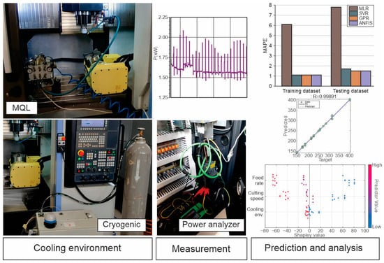
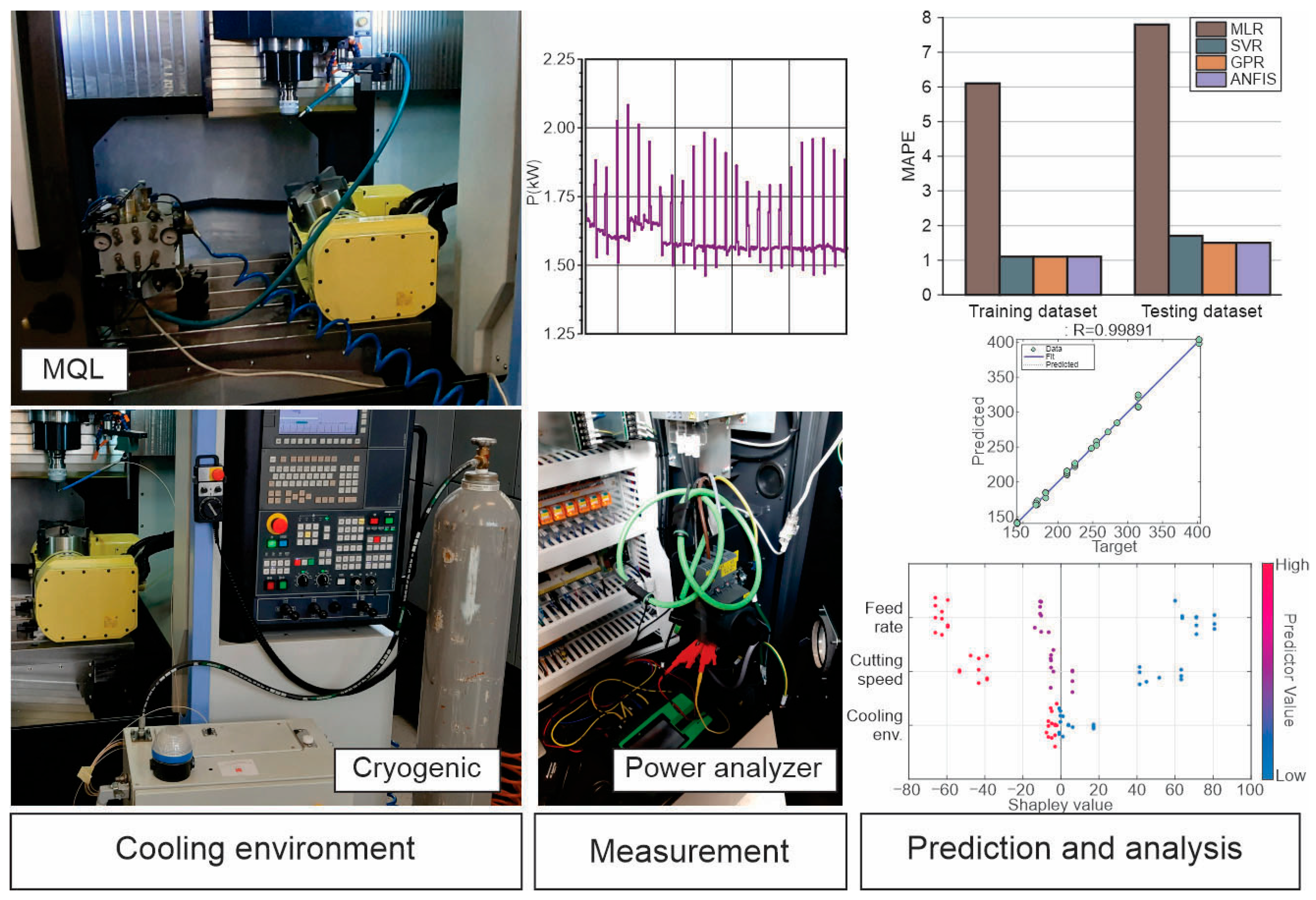
The ML models reported in the literature mostly addressed conventional flood machining. There is barely any available knowledge about predicting the energy consumption during machining under different cooling conditions. The selection of a cooling method, together with energy efficiency, is broadly recognized as a major factor in the transition towards a sustainable machining process. High-performance alloys, such as Ti-based alloys, consume more specific cutting energy compared to steel, aluminum, etc. Moreover, machining complexity, that is, the difficulty of machining the surface, also has an impact on machine tool energy consumption. Theoretically, the main problems with ball-end milling operations are the poor cutting conditions at the tool tip, the unfavorable transfer of generated heat, difficult chip disposal, and the low material removal rate (MRR). The present research is a continuation and an extension of our earlier studies. In particular, we analyzed and determined optimal settings of control parameters for the minimization of SEC as an objective function [25] and presented a multi-objective parameter optimization model integrating the machining responses, such as surface roughness, microhardness, energy consumption, and productivity, and sustainability metrics, such as environmental impact, operator’s health and safety, and waste management [26]. Hence, the current study reveals the potential of ML models in promoting sustainable machining of difficult-to-cut material Ti-6Al-4V, which is the most widely used commercial Ti-based alloy. This alloy accounts for more than half of global production and is utilized in 80% of aerospace and medical applications. The four ML-based models, namely, multiple linear regression (MLR), support vector regression (SVR), Gaussian process regression (GPR), and adaptive network-based fuzzy inference system (ANFIS), were developed to predict specific energy consumption (SEC) in ball-end milling of Ti6-Al4-V alloy under MQL and cryogenic machining conditions. Figure 1 shows the methodology of the present research work. Initially, two eco-friendly cooling environments, namely MQL and cryogenic cooling, along with other machining parameters, were utilized to investigate their effects on SEC. Subsequently, MLR, SVR, GPR, and ANFIS ML models were employed to develop predictive models. Ultimately, the prediction performance of the ML models was analyzed.
Figure 1.
Experimental setups and modeling procedure.
2. Experimental Work
In this study, the Ti-based alloy Ti-6Al-4V was used as the workpiece material. Ti-6Al-4V is currently the most studied Ti-based alloy worldwide, with a large number of publications. This alloy is known as one of the most difficult-to-cut alloys due to its material properties. The chemical composition (wt.%) and mechanical properties of the considered alloy are presented in Table 1.
Table 1.
Chemical composition and mechanical properties of Ti6-Al4-V alloy.
The carbide ball-nosed end mill was used for experimentation; its geometric parameters are as follows: number of cutting edges n = 2, diameter d = 10 mm, flute length l = 16 mm, helix angle β = 30°, and rake angle γ = 30°. As a consequence of the zero effective cutting speed at the tool axis, the tool was rotated 20° relative to its vertical position (inclination angle ζ = 20°) to avoid plastic deformation of the machined layer.
The experimental trials were conducted using a Taguchi L36 (21 32) orthogonal-array design, which ensures statistical balance and independent estimation of factor effects while reducing the total number of experiments. The trials were performed on a 5-axis CNC machining center, Doosan NX 6500 II (DN Solutions, Seoul, Republic of Korea), equipped with a Fanuc controller (Fanuc Corporation, Oshino, Japan). The technical specifications of the machine tool include a 20,000 rpm maximum spindle speed and a motor power of 22 kW. A carbide ball-nosed end mill model S501 (Dormer Pramet, Šumperk, Czech Republic) with two flutes was selected for all machining trials. This specific tool geometry includes a diameter of 10 mm and a flute length of 19 mm, characterized by a 30° helix angle and a 10° rake angle.
Three controllable factors, two numerical (cutting speed—vc and feed per tooth—ft) and one categorical—cooling condition (MQL and cryogenic)—were considered during the experimental investigation. The experimental setup utilized an MQL system comprising a compressed air source, lubricant tank, flow control unit, and spray nozzle. The air pressure (0.6 MPa) and flow rate (60 mL/h) remained constant. A conventional cryogenic cooling configuration, comprising a CO2 source, pressure regulation, and flow control, was employed in this study. For machining operations, CO2 was supplied at a delivery pressure of 5.7 MPa and a flow rate of 12 kg/h through a 0.8 mm diameter nozzle.
The specific energy consumption (SEC) was calculated as the ratio of cutting power (P) to material removal rate (MRR). The power disturbance analyzer MAVOWATT (Dranetz-BMI) was used to monitor the cutting power during the machining trials. This instrument is capable of recording various electrical parameters, including active power, voltage, current, and frequency. The results of the experimentation are shown in Table 2.
Table 2.
DOE with the experimental results.
3. Machine Learning Methods
3.1. Multiple Linear Regression
One of the most popular machine learning techniques is regression analysis. Modeling the relationship between one or more independent variables (predictors) and a dependent variable (response) in order to estimate future values is the main objective of regression analysis. The simplest method for the regression task is linear regression (LR), whereas multiple linear regression (MLR) is an extension of simple linear regression, as it involves multiple variables.
The general expression for the MLR model is given by the following equation:
where y is a dependent variable, x1, x2, …, xk are independent variables, β0 is a constant coefficient, β1, β2, …, βk are the regression coefficients, and ε is the random error of viewing number i for i = 1,2, …, n units of observations.
3.2. Support Vector Regression
Based on the statistical learning theory, Vapnik introduced a machine learning algorithm called the support vector machine (SVM). Originally developed to solve pattern recognition problems, in recent years, SVM has been very successfully applied for solving a variety of learning and prediction problems as well. As a regression version of SVM, support vector regression (SVR) is an efficient and powerful algorithm for dealing with nonlinear regression problems [27]. The SVR model employs a training data set , where represents input values, are the corresponding output values, and m is the total number of samples. The objective of the regression problem is to identify a function f(x) that, for all the training data, deviates no more than ε from the actually obtained targets yi.
The generic regression function f(x) can be formulated as follows:
where ϕ(x) denotes the nonlinear transformation of the input pattern x from Rn to the high-dimensional feature space, whereas w and b indicate the weight vector and bias term, respectively.
The weight vector w and bias term b are obtained by minimizing the regularized risk function:
where C is a regularized constant, and Lε(y, f(x)) is the loss function. Vapnik presented a general type of loss function, namely the ε-insensitive loss function, defined as follows:
where ε is the difference between values computed from the regression function and actual values.
Introducing two slack variables (ξi and ξi*) to measure errors outside the ε-tube, Equation (3) is transformed into the following constrained form
subject to
By adding Lagrangian multipliers (αi, αi*, βi, and βi*), Equation (5) is then reformulated as follows:
By applying Karush–Kuhn–Tucker conditions to Equation (6), the following dual form of the optimization problem is obtained:
subject to
Finally, by solving the above optimization problem and determining values of the Lagrange multipliers, an optimal solution of the weight vector and regression function can be obtained as follows:
where K(xi, xj) is the kernel function that maps the input data to a feature space, satisfying K(xi, xj) = ϕ(xi)·ϕ(xj). Every function that satisfies Mercer’s condition can be used as a kernel function. There are several kernel functions suggested in the literature, such as the radial basis function, polynomial function, and linear function. The radial basis function (RBF) can be expressed mathematically as
where σ is the kernel width parameter.
3.3. Gaussian Process Regression
Gaussian process regression (GPR) was initially proposed by Williams and Rasmussen [28]. GPR is highly adaptable and is capable of handling a wide range of complex issues, including nonlinearity, limited sample sizes, and high dimensionality.
Suppose that D = {X, y} is a set of training data, where X = [x1, x2, …, xn] is an input vector in Rd and y = [y1, y2, …, yn] is a vector containing scalar training outputs yi in R. The output yi might be presumed to include mean-zero additive Gaussian noise with variance σn2, which is described as p(εi) = N(0, σn2). Moreover, if the outputs are independent and identically distributed, each observation yi can be viewed as related to an underlying function f(x) through a Gaussian noise model:
The joint distribution over the outputs is a zero-mean Gaussian and corresponds to the following equation:
where f (x) = [ f1, f2, …, fn]T is a vector of latent functions, K(x, xʹ) is the covariance (kernel) matrix with elements Kij(xi, xj), the term σn2I represents the Gaussian noise, and I is the identity matrix.
The objective of the GPR algorithm is to determine the predicted outputs f* with probabilistic confidence levels for the training samples and a set of test points X*. The following equation can be employed to formulate a prior joint distribution of the training outputs (f) and test outputs (f*):
The independent likelihood can be defined using the following equation:
The Gaussian predictive distribution can be determined by obtaining the posterior distribution, assuming that the hyperparameters involved in K were previously acquired from the following training data:
where the mean µ and the variance σ are defined as
The covariance between the two input feature vectors, xi and xj, is determined by the squared exponential kernel function:
where σs2, which is typically initialized to 1, is the signal variance that indicates the overall magnitude of the covariance value, M is a diagonal matrix M = diag{l1, l2, …, lm}, l are scaling factors, and δij is Kronecker’s delta function, which is used to define the noise variance σn2 in the covariance value.
The hyperparameters of the Gaussian process are the kernel function parameters denoted by θ = [M, σs, σn]. These hyperparameters can be learned by maximizing the logarithmic likelihood function of the training outputs:
where the logarithmic term can be defined as follows:
Different optimization techniques, such as Bayesian optimization, evolutionary algorithms, etc., can be used to address this nonlinear optimization problem.
3.4. Adaptive Neuro-Fuzzy Nference System (ANFIS)
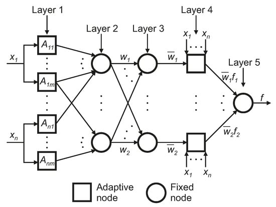
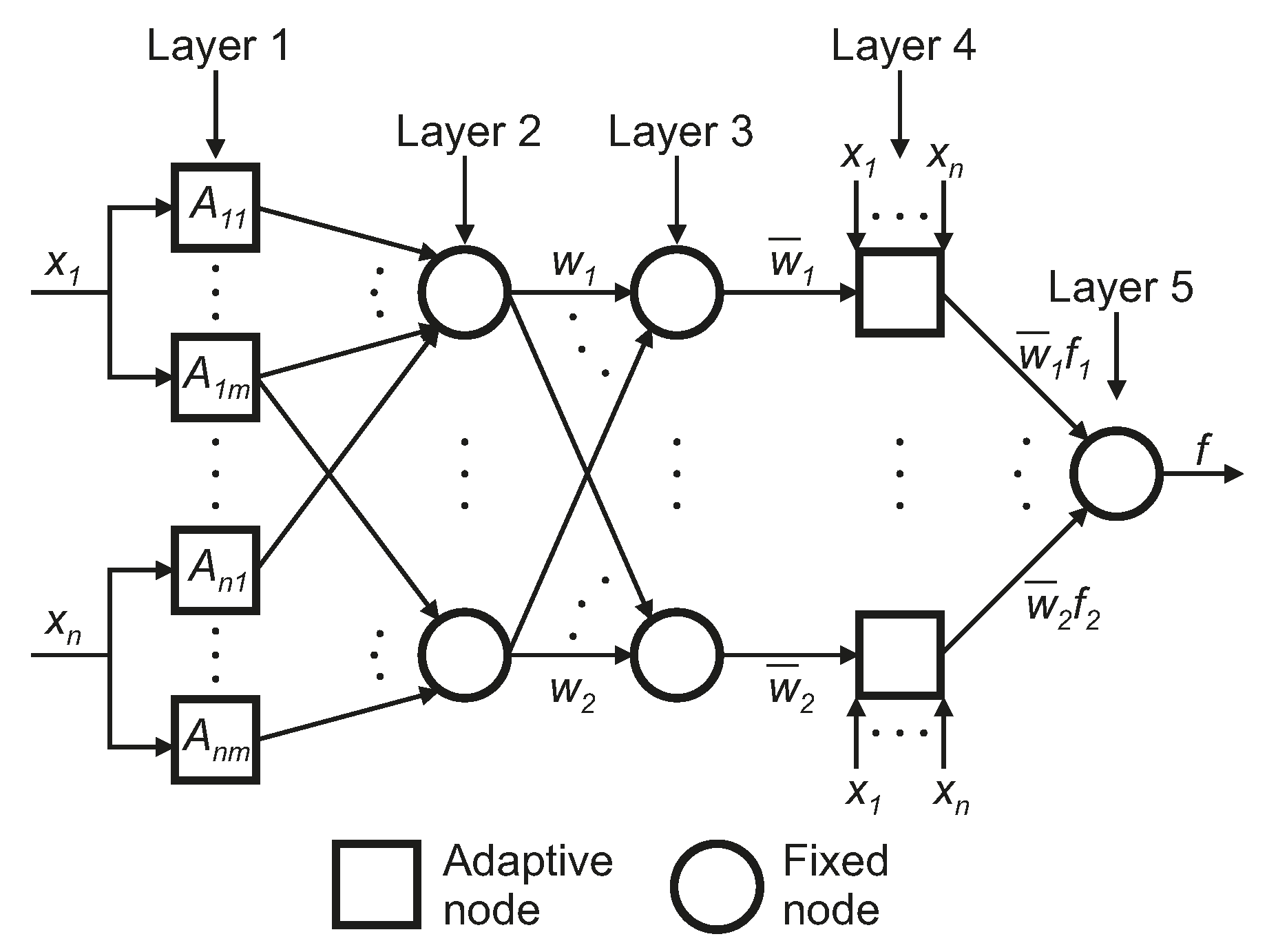
The adaptive network-based fuzzy inference system (ANFIS) is one of the most popular soft computing techniques originally introduced by Jang [29]. ANFIS merges the knowledge representation of a fuzzy inference system (FIS) with artificial neural networks (ANN) learning capabilities, consequently providing the advantages of both methods. As depicted in Figure 2, the typical ANFIS architecture has five layers. For the purpose of simplification, it is assumed that the FIS has two inputs (x and y) and one output (f).
Figure 2.
The architecture of ANFIS.
For a first-order Takagi–Sugeno fuzzy inference model, the rule base with two fuzzy if-then rules is defined as follows:
where Ai and Bi are the fuzzy sets that represent linguistic labels, and pi, qi, and ri are design parameters that are determined through the training process.
The nodes and layers functions are described below.
Layer 1: this layer contains adaptive nodes, denoted by squares, with the node function described as follows:
where µ(x) and µ(y) represent the membership functions (MFs) of the corresponding linguistic variable sets Ai and Bi-2, respectively. In general, several types of MFs can be employed, such as triangular, trapezoidal, Gaussian, generalized bell-shaped, etc.
Layer 2: in this layer, every node is a fixed node, marked by a circle, and is used to multiply the input signals to serve as an output signal:
Layer 3: the third layer also contains fixed nodes, with the node function to normalize the firing strength from the previous layer as follows:
Layer 4: in the fourth layer, every node is an adaptive node, with the node function defined as
Layer 5: in this layer, there is only a single fixed node that carries out the summation of all incoming signals. The output of this layer represents the overall output of the model and is defined by
4. Evaluation Metrics
The performance of the ML models was analyzed and evaluated in terms of the following measures: normalized mean absolute error (nMAE), mean absolute percentage error (MAPE), normalized root mean square error (nRMSE), maximum absolute percentage error (maxAPE), coefficient of determination (R2), and Willmott’s index of agreement (IA). These statistical metrics are defined as follows:
where n is the number of training patterns, Oi and Pi are the observed and predicted values of the ith training pattern, respectively, and is the observed mean value.
5. Machine Learning Models Development
In this part of the study, four ML models have been developed to predict SEC in ball-end milling of Ti6-Al4-V alloy under MQL and cryogenic machining conditions. Each model has three input parameters: cooling conditions, cutting speed, and feed per tooth, whereas one output of the model is SEC. Firstly, the database is randomly divided into two sets: a training data set and a testing data set. Thus, 28 data sets gathered from the experiments, under both environments, have been selected for the purpose of training ML models. Then, the remaining eight data sets have been employed for testing purposes in order to verify the accuracy of the predicted values obtained by ML models. The present study is based on a dataset of 36 samples, which, although small in size, is usual for experimental studies involving SEC measurements. Collecting large datasets in this domain is very difficult because data collection is costly and time-consuming. In order to ensure that this relatively small dataset does not compromise the reliability of the ML model analysis, each measurement was performed under carefully controlled operating conditions, resulting in high data fidelity and a favorable signal-to-noise ratio. Moreover, the dataset covers the practical range of the machining variables, guaranteeing representative coverage of the operating domain. In order to ensure reliable comparison of selected ML models under small sample settings, 10 k-fold cross-validation was employed. This approach partitions the dataset into ten subsets, and each fold was used nine times for training and once for testing. In order to assess the stability of the model, the standard deviation across folds was used to quantify variability. The low dispersion observed indicates stable model performance and limited overfitting. This methodology was integrated into the development of each ML model to maximize data utility and minimize predictive variance. The use of compact model structures and regularization-based ML models, such as SVR, GPR, and ANFIS, further supports stable learning under limited sample conditions.
First, from a set of experimentally obtained data, an MLR model was developed in order to evaluate SEC as a function of machining parameters, such as cutting speed (vc), and feed per tooth (ft) in MQL and cryogenic-assisted milling as follows:
The analysis of variance (ANOVA) was employed to validate the significance of the developed MLR model. Results of ANOVA revealed that the developed model is suitable, irrespective of the machining condition (cryogenic or MQL).
For the SVR model, the type of kernel function, the kernel function parameter, the cost function parameter (C), and the value of ε for the ε-insensitive loss function are the most influential factors, which have a major effect on the model’s performance. Numerous techniques, including gradient-based optimization, genetic algorithm, grid search, etc., can be used for the process of fine-tuning the hyperparameters to enhance a model’s performance. In the context of ML model hyperparameter optimization, among the various hyperparameter optimization methods, in this study, the Bayesian optimization algorithm was used. The SVR model was analyzed using various kernel functions, such as linear, radial basis function (RBF), and polynomial, to determine the most suitable one. Then, the model hyperparameters C, γ, and ε were tuned using the Bayesian optimization algorithm for all kernels. In order to maintain a compromise between computational feasibility and hyperparameter space exploration, the number of iterations for Bayesian optimization was set to 30. The SVR model’s quality was assessed using the cross-validated mean squared error, ensuring generalization across the training dataset. The hyperparameters C, γ, and ε were optimized over predefined ranges [10−2, 103], [10−3, 102], and [10−3, 10−1], respectively. The optimal SVR model was identified as follows: RBF kernel: C = 101, γ = 0.2, and ε = 0.01.
The output performance of the GPR model is also highly dependent on the choice of hyperparameters. For this purpose, the present study introduces a Bayesian optimization for identifying the most significant hyperparameters of the GPR-based model, including the kernel function, basis function, and initial value for the noise standard deviation. The number of iterations for Bayesian optimization is set to 30, identical to the SVR model, to ensure a fair comparison. Hyperparameter tuning for GPR models was based on the cross-validation mean squared error computed on the training dataset. The hyperparameter configuration that corresponds to the best GPR model was an exponential kernel function, a constant basis function, and a sigma value of 0.01.
Finally, the first-order Takagi–Sugeno fuzzy ANFIS model was developed. The proposed ANFIS model is a multi-input single-output model, with three input parameters: cooling conditions, cutting speed, and feed per tooth, whereas one output of the model is SEC. The MFs of cooling conditions within the ANFIS architecture were divided into two areas, i.e., small (S) and large (L), while the MFs of cutting speed and feed per tooth were divided into three areas, i.e., small (S), medium (M), and large (L). Different types of MFs were used in training ANFIS to predict specific cutting energy, and the Gaussian MF was selected as optimal. Furthermore, linear output MFs type were employed for the ANFIS training process in this study. The number of maximum iterations and the number of epochs were 30 and 10, respectively. The initial step was 0.01, and the step size decreasing rate was 0.8, whereas 1.1 was the step size increasing rate, and 0 was the error target assigned. ANFIS MFs were initialized using a data-driven partitioning of the input space rather than random initialization. Finally, a steepest-descent method (backpropagation for all parameters) and a hybrid method consisting of backpropagation for the parameters associated with the input MFs and least squares estimation for the parameters associated with the output MFs were used for updating the MF parameters of a fuzzy inference system.
6. Results and Discussion
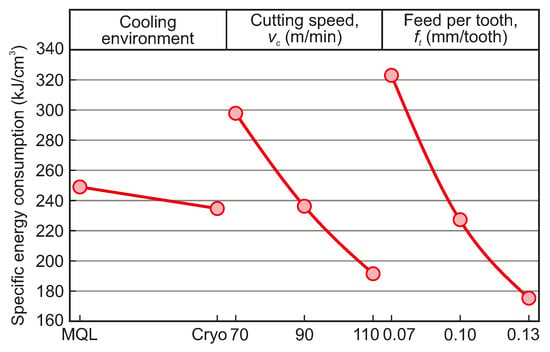
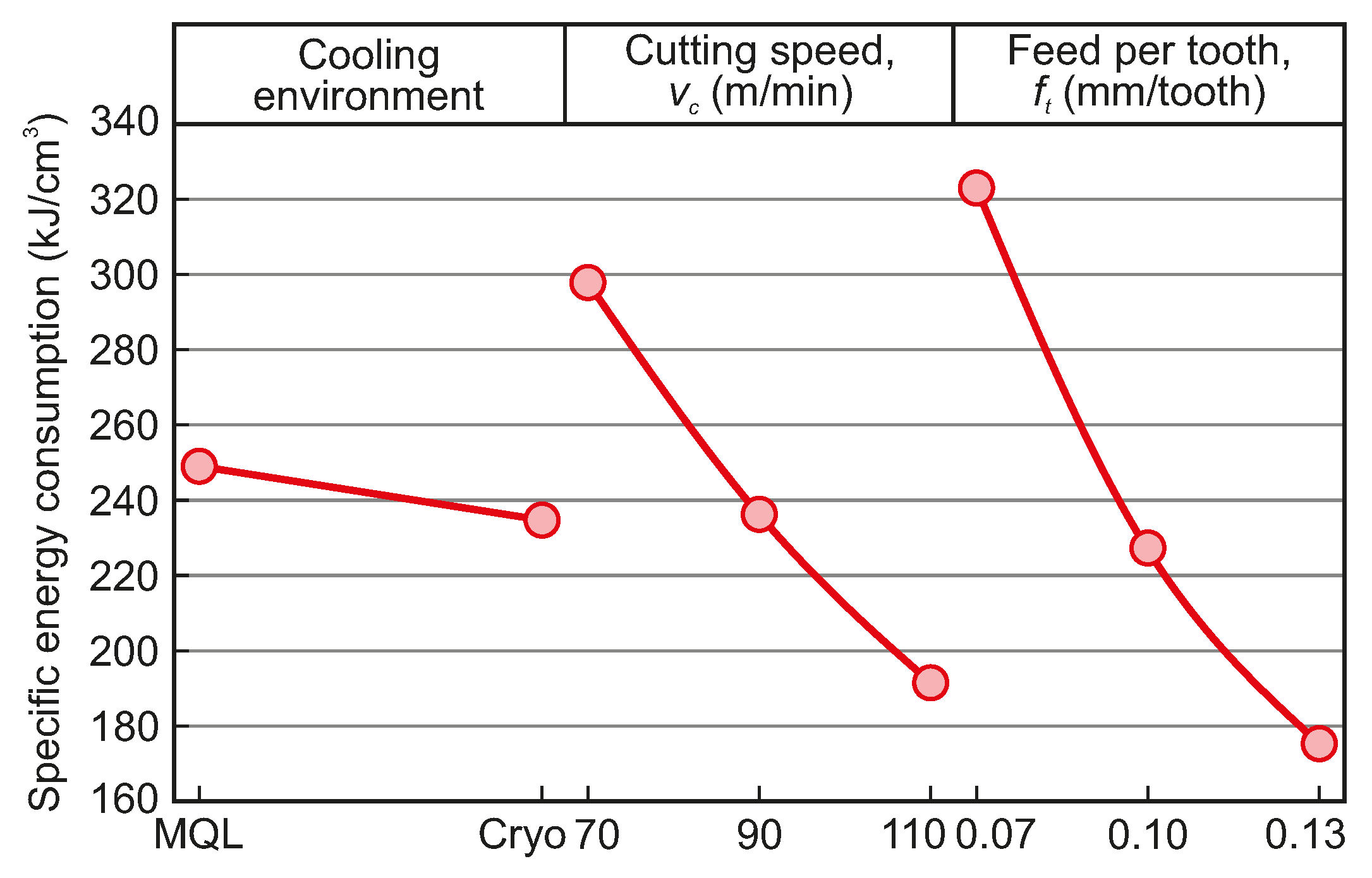
Prior to presenting the ML results, a main effect plot (Figure 3) was employed to analyze how process parameters influence SEC. Moreover, from this plot, the optimal levels of process parameters can also be determined. The graphical analysis indicates that feed per tooth is the most influential factor on SEC, followed by cutting speed and the cooling environment. The results demonstrate that SEC is primarily influenced by feed per tooth and cutting speed, with SEC decreasing as these two parameters are increased. Additionally, the results indicate that cooling environments have a marginal impact on SEC. Finally, the results indicate that the combination of cryogenic cooling and the highest settings for both feed per tooth and cutting speed yields the optimal process configuration. This observation is attributable to the superior heat dissipation provided by cryogenic cooling, which minimizes cutting forces and indirectly energy consumption. Simultaneously, increasing the feed per tooth and cutting speed enhances the MRR, which shortens the overall machining time.
Figure 3.
Main effects plot on SEC.
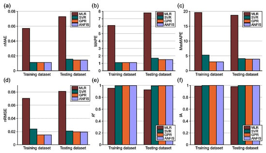
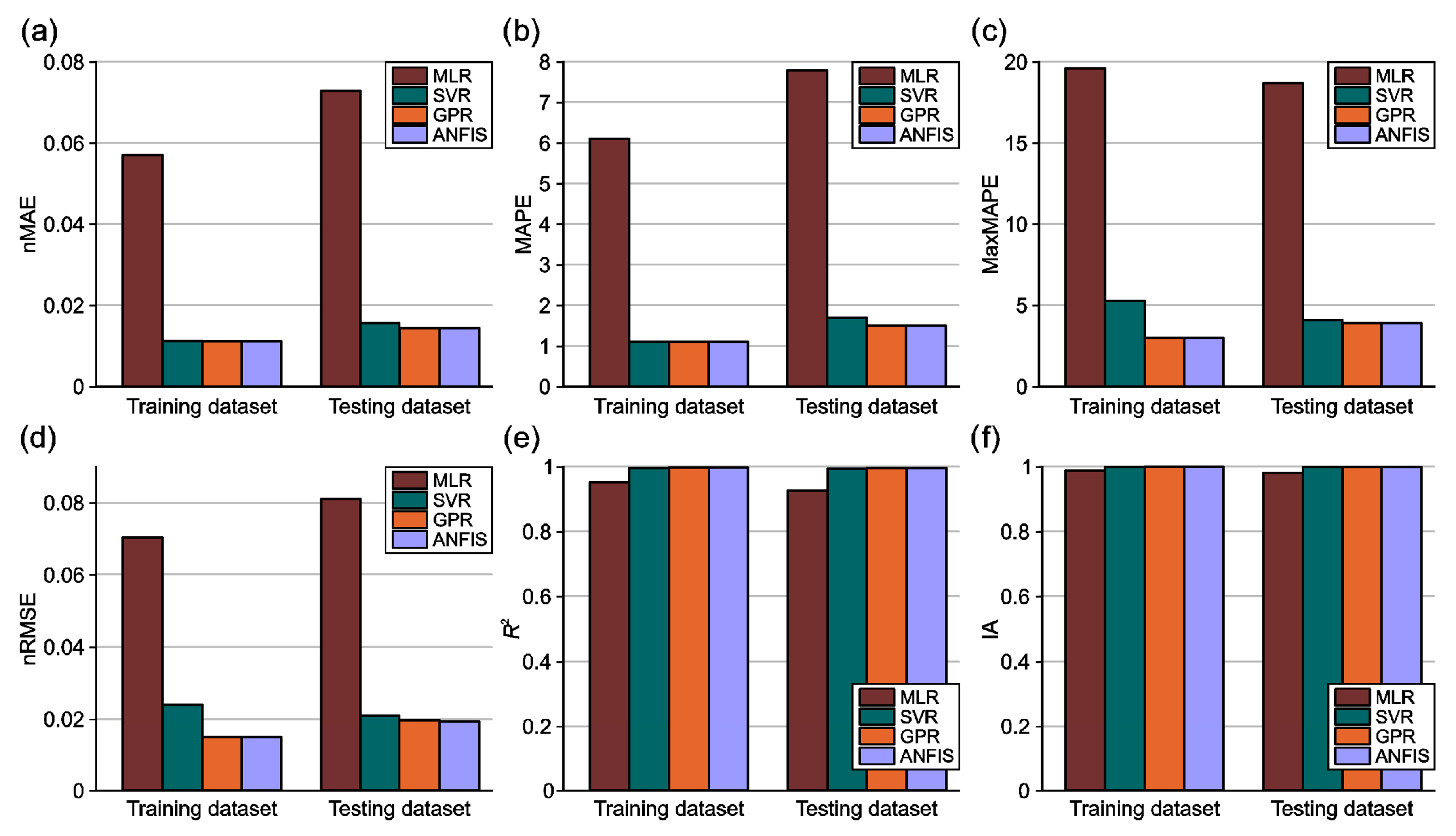
The subsequent paragraphs explore the training and testing results of four ML models, including MLR, SVR, GPR, and ANFIS, to investigate their predictive abilities of SEC in the milling of Ti-based superalloy under MQL and cryogenic environments. The comparison was done across training and testing datasets using nMAE, MAPE, maxAPE, nRMSE, R2, and IA as the performance measures. Table 3 and Figure 4 illustrate the prediction results of the different ML models using various evaluation measures. According to our investigation, none of the assessed models show a statistically significant difference in prediction performance between the cryogenic and MQL datasets.
Table 3.
Analysis of different ML models using various evaluation metrics.
Figure 4.
Performance results of explored ML models for test dataset.
The training phase. The results show that the proposed ANFIS model performs the best in terms of nMAE. The values of nMAE of ANFIS, GPR, SVR, and MLR models are 0.0111, 0.0112, 0.0113, and 0.0571, respectively. The SVR, GPR, and ANFIS models yielded identical values for MAPE (MAPE = 1.1), followed by MLR (MAPE = 6.1). Lowest maxAPE values for the training dataset were obtained for the GPR and ANFIS models (maxAPE = 3), followed by SVR (maxAPE = 5.3) and MLR (maxAPE = 19.6). In terms of nRMSE, the GPR and ANFIS models revealed superiority (nRMSE = 0.0150) over SVR (nRMSE = 0.0240) and MLR (nRMSE = 0.0704). Good agreement between the experimental and predicted results for the GPR and ANFIS models was obtained (the coefficient of determination was 0.9978), followed by the SVR and MLR, with coefficients of determination of 0.9960 and 0.9519, respectively. Finally, the results of Willmott’s index of agreement (IA) revealed superior performance for the GPR and ANFIS models (IA = 0.9995), followed by SVR (IA = 0.9990) and the MLR model (IA = 0.9875).
The testing phase. The GPR and ANFIS models have achieved the best accuracy with an nMAE value of 0.0144, followed by SVR (nMAE = 0.0156) and the MLR model (nMAE = 0.0729). The GPR and ANFIS models once more surpassed the other models with the lowest MAPE of 1.5 and maxAPE of 3.9. The SVR and MLR models had MAPE values of 1.7 and 7.8, respectively, and maxAPE values of 4.1 and 18.7, respectively. The ANFIS model exhibited superior prediction performance in terms of nRMSE, followed by the GPR, SVR, and MLR models. The nRMSE values for the ANFIS, GPR, SVR, and MLR models were obtained as 0.0194, 0.0196, 0.0210, and 0.0810, respectively. The ANFIS model attained the greatest R-squared value of 0.9957, indicating that the model has strong prediction ability. It can be seen that the GPR and SVR models also had high R-squared values of 0.9956 and 0.9950, respectively, followed by the MLR model with an R-squared value of 0.9254. The GPR and ANFIS models both achieved the highest IA values of 0.9989, followed by the SVR (IA = 0.9987) and MLR model (IA = 0.9809).
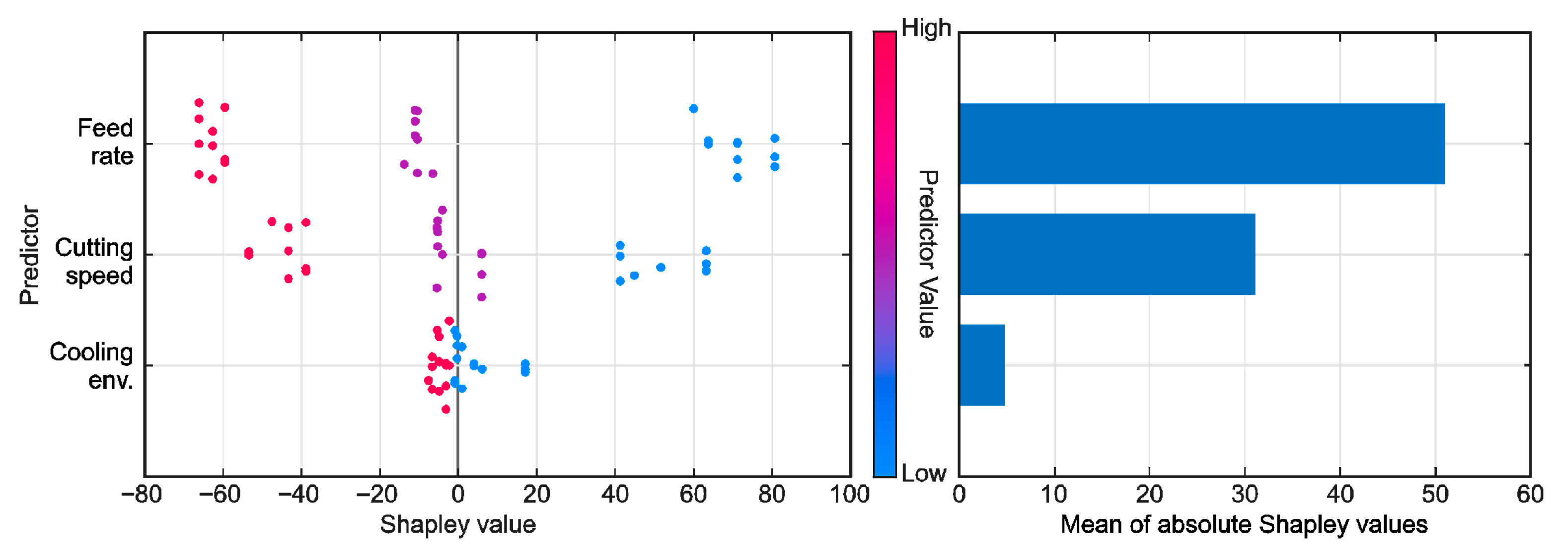
The SHAP (Shapley additive explanations) method was employed to quantify the individual contribution of each input feature to the GPR model output. The SHAP analysis results designate feed per tooth and cutting speed as the most significant contributors to SEC (Figure 5). Contrary to this, the cooling environment demonstrates a marginal impact. This ranking confirms that SEC in ball-end milling is primarily governed by process parameters associated with chip formation and cutting mechanics, whereas the cooling method has a limited effect on SEC within the investigated range.
Figure 5.
Feature importance ranking based on SHAP analysis.
According to the values of nMAE, MAPE, maxAPE, nRMSE, R2, and IA obtained by each ML model in the training and testing phase, the prediction efficiency of models increases in the order: ANFIS > GPR > SVR > MLR.
The improved performance of the ANFIS, GPR, and SVR models can be justified primarily because SEC reveals notable nonlinear behavior and strong interactions between machining parameters. MLR presumes a strictly linear relationship, which cannot capture these effects properly. On the other hand, ANFIS represents them through adaptive fuzzy rules, GPR through flexible covariance kernels, and SVR through nonlinear kernel mappings. In addition, because ANFIS, GPR, and SVR models incorporate built-in regularization that improves the generalization ability of the model, they perform better under small sample datasets, enhancing their adequacy for SEC prediction. Accordingly, the nonlinear ML models are more compatible with the complex physical characteristics of the ball-end milling process and provide more accurate predictions. Despite the aforementioned disadvantages, the MLR model retains advantages such as low computational cost and high interpretability.
7. Conclusions
The present study demonstrates the effectiveness of four ML models, namely, multiple linear regression (MLR), support vector regression (SVR), Gaussian process regression (GPR), and adaptive network-based fuzzy inference system (ANFIS), in predicting specific energy consumption (SEC) in the milling of Ti-Al6-4V alloy under sustainable cooling conditions. The number of 28 data sets gathered from the experiments has been randomly selected for the purpose of training different ML models. The remaining eight data sets have been employed for testing purposes in order to verify the accuracy of the predicted values obtained by ML models. The prediction accuracy of each ML model was assessed with statistical indicators such as normalized mean absolute error (nMAE), mean absolute percentage error (MAPE), normalized root mean square error (nRMSE), maximum absolute percentage error (maxAPE), coefficient of determination (R2), and Willmott’s index of agreement (IA).
It is possible to note that among the analyzed ML models for the training dataset, ANFIS demonstrated the best predictive capability in all evaluation metrics. In addition, the GPR model demonstrated a marginally elevated nMAE value of 0.0112, indicating similar performance to ANFIS, yielding identical values for other evaluation indicators. It’s worth mentioning that the SVR model also performed well in all performance indicators, validating a high degree of alignment between the experimental and predicted values of SEC. The MLR model, on the other hand, had the poorest predictive outcomes.
A similar conclusion can be derived by comparing evaluation metrics for the test dataset. The comparative analysis of all ML models in the research revealed that the ANFIS model is optimal in terms of all performance metrics. The GPR model in the present study showed very similar performance to the optimal ANFIS model. According to the performance metrics, the GPR model demonstrated negligibly elevated values for two metrics, namely, nRMSE and R2. Although the predictive performance of the SVR model is slightly poorer compared to ANFIS and GPR, it still represents a very accurate predictive model with excellent performance metrics. Finally, the MLR model exhibited the poorest performance, not only in the training set but also in the testing set, indicating its limited predictive capability.
Among the evaluated ML models, ANFIS, GPR, and SVR models exhibited superior predictive capability because of their ability to capture nonlinear and interacting effects in complex processes such as ball-end milling, even if they require hyperparameter tuning and provide lower interpretability than the MLR model. The results confirm that the proposed ML models successfully achieved the aim of accurately predicting SCE in ball-end milling of Ti-6Al-4V, while providing interpretable insight into the dominant influence of feed per tooth and cutting speed. The developed prediction models can be directly used as decision-support tools in machining of difficult-to-cut materials operations to estimate specific energy consumption under alternative cooling conditions. This approach supports sustainable machining by minimizing trial-and-error testing, saving energy consumption, and enabling informed parameter adjustments based on reliable model predictions.
Author Contributions
Conceptualization, D.C., D.K. and M.Z.; methodology, D.C., S.T. and F.P.; validation, D.C., D.K. and B.S.; investigation, D.K., M.Z., F.P., S.T. and D.V.; formal analysis, D.C., D.K., B.S., S.T. and F.P.; resources, D.K., M.Z. and F.P.; writing—original draft preparation, D.C. and D.K.; writing—review and editing, D.C., D.K., S.T., D.V., M.Z., F.P. and D.K.; visualization, D.C., S.T. and D.K., supervision, M.Z. and F.P.; project administration, D.K., S.T. and B.S., funding acquisition, D.K., D.V., M.Z. and F.P. All authors have read and agreed to the published version of the manuscript.
Funding
This research received no external funding.
Data Availability Statement
The original contributions presented in this study are included in the article. Further inquiries can be directed to the corresponding author.
Conflicts of Interest
The authors declare no conflicts of interest.
References
- Kramar, D.; Cica, D. Experimental investigation and optimization of tool life in high-pressure jet-assisted turning of Inconel 718. Metals 2025, 15, 477. [Google Scholar] [CrossRef] [Scilit]
- Zhou, Z.; Yao, B.; Xu, W.; Wang, L. Condition monitoring towards energy-efficient manufacturing: A review. Int. J. Adv. Manuf. Technol. 2017, 91, 3395–3415. [Google Scholar] [CrossRef] [Scilit]
- Yi, Q.; Ji, Q.; Zhu, D.; Jin, Y.; Li, L. Design optimization of lathe spindle system for optimum energy efficiency. J. Clean. Prod. 2020, 250, 119536. [Google Scholar] [CrossRef] [Scilit]
- Cai, W.; Liu, F.; Zhou, X.; Xie, J. Fine energy consumption allowance of workpieces in the mechanical manufacturing industry. Energy 2016, 114, 623–633. [Google Scholar] [CrossRef] [Scilit]
- Yoon, H.S.; Kim, E.S.; Kim, M.S.; Lee, J.Y.; Lee, B.G. Towards greener machine tools—A review on energy saving strategies and technologies. Renew. Sustain. Energy Rev. 2015, 48, 870–891. [Google Scholar] [CrossRef] [Scilit]
- Wang, H.; Zhong, R.Y.; Liu, G.; Mu, W.L.; Tian, X.; Leng, D. An optimization model for energy-efficient machining for sustainable production. J. Clean. Prod. 2019, 232, 1121–1133. [Google Scholar] [CrossRef] [Scilit]
- Shin, S.J.; Kim, Y.M.; Meilanitasari, P. A holonic-based self-learning mechanism for energy—Predictive planning in machining processes. Processes 2019, 7, 739. [Google Scholar] [CrossRef] [Scilit]
- He, Y.; Wu, P.; Li, Y.; Wang, Y.; Tao, F.; Wang, Y. A generic energy prediction model of machine tools using deep learning algorithms. App. Energy 2020, 275, 115402. [Google Scholar] [CrossRef] [Scilit]
- Cao, J.; Xia, X.; Wang, L.; Zhang, Z.; Liu, X. A novel CNC milling energy consumption prediction method based on program parsing and parallel neural network. Sustainability 2021, 13, 13918. [Google Scholar] [CrossRef] [Scilit]
- Liu, Z.; Guo, Y. A hybrid approach to integrate machine learning and process mechanics for the prediction of specific cutting energy. CIRP Ann. Manuf. Technol. 2018, 67, 57–60. [Google Scholar] [CrossRef] [Scilit]
- Zhang, M.; Zhang, H.; Yan, W.; Jiang, Z.; Zhu, S. An integrated deep-learning-based approach for energy consumption prediction of machining systems. Sustainability 2023, 15, 5781. [Google Scholar] [CrossRef] [Scilit]
- Ross, N.S.; Rai, R.; Ananth, M.B.J.; Srinivasan, D.; Ganesh, M.; Gupta, M.K.; Korkmaz, M.E.; Krolczyk, G.M. Carbon emissions and overall sustainability assessment in eco-friendly machining of Monel-400 alloy. Sustain. Mater. Technol. 2023, 37, e00675. [Google Scholar] [CrossRef] [Scilit]
- Sealy, M.P.; Liu, Z.Y.; Zhang, D.; Guo, Y.B.; Liu, Z.Q. Energy consumption and modeling in precision hard milling. J. Clean. Prod. 2016, 135, 1591–1601. [Google Scholar] [CrossRef] [Scilit]
- Brillinger, M.; Wuwer, M.; Hadi, M.A.; Haas, F. Energy prediction for CNC machining with machine learning. CIRP J. Manuf. Sci. Technol. 2021, 35, 715–723. [Google Scholar] [CrossRef] [Scilit]
- Lu, F.; Zhou, G.; Zhang, C.; Liu, Y.; Chang, F.; Xiao, Z. Energy-efficient multi-pass cutting parameters optimisation for aviation parts in flank milling with deep reinforcement learning. Robot. Comput. Integr. Manuf. 2023, 81, 102488. [Google Scholar] [CrossRef] [Scilit]
- Nugrahanto, I.; Gunawan, H.; Chen, H.Y. Innovative approaches to sustainable computer numeric control machining: A machine learning perspective on energy efficiency. Sustainability 2024, 16, 3569. [Google Scholar] [CrossRef] [Scilit]
- Selvaraj, V.; Xu, Z.; Min, S. Intelligent operation monitoring of an ultra-precision CNC machine tool using energy data. Int. J. Precis. Eng. Manuf. Green Technol. 2023, 10, 59–69. [Google Scholar] [CrossRef] [Scilit]
- Awan, M.R.; Rojas, H.A.G.; Hameed, S.; Riaz, F.; Hamid, S.; Hussain, A. Machine learning-based prediction of specific energy consumption for cut-off grinding. Sensors 2022, 22, 7152. [Google Scholar] [CrossRef] [Scilit]
- Yurtkuran, H.; Korkmaz, M.E.; Gupta, M.K.; Yilmaz, H.; Günay, M.; Vashishtha, G. Prediction of power consumption and its signals in sustainable turning of PH13-8Mo steel with different machine learning models. Int. J. Adv. Manuf. Technol. 2024, 133, 2171–2188. [Google Scholar] [CrossRef] [Scilit]
- Bhattacharya, S.; Chakraborty, S. Prediction of responses in a CNC milling operation using random forest regressor. Facta Univ. Ser. Mech. Eng. 2023, 21, 685–700. [Google Scholar] [CrossRef] [Scilit]
- Farooq, M.U.; Kuma, R.; Khan, A.; Singh, J.; Anwar, S.; Verma, A.; Haber, R. Sustainable machining of Inconel 718 using minimum quantity lubrication: Artificial intelligence-based process modelling. Heliyon 2024, 10, e34836. [Google Scholar] [CrossRef] [Scilit]
- Korkmaz, M.E.; Gupta, M.K.; Yilmaz, H.; Ross, N.S.; Boy, M.; Sivalingam, V.K.; Chan, C.K.; Raman, J. Towards specific cutting energy analysis in the machining of Inconel 601 alloy under sustainable cooling conditions. J. Mater. Res. Technol. 2023, 27, 4074–4087. [Google Scholar] [CrossRef] [Scilit]
- Xu, Z.; Selvaraj, V.; Min, S. State identification of a 5-axis ultra-precision CNC machine tool using energy consumption data assisted by multi-output densely connected 1D-CNN model. J. Intell. Manuf. 2024, 35, 147–160. [Google Scholar] [CrossRef] [Scilit]
- Aslan, A. Machine learning models and machinability analysis for comparison of various cooling and lubricating mediums during milling of Hardox 400 steel. Tribol. Int. 2024, 198, 109860. [Google Scholar] [CrossRef] [Scilit]
- Tesic, S.; Cica, D.; Borojevic, S.; Sredanovic, B.; Zeljkovic, M.; Kramar, D.; Pusavec, F. Optimization and prediction of specific energy consumption in ball-end milling of Ti-6Al-4V alloy under MQL and cryogenic cooling/lubrication condition. Int. J. Precis. Eng. Manuf. Green Technol. 2022, 9, 1427–1437. [Google Scholar] [CrossRef] [Scilit]
- Cica, D.; Tesic, S.; Markovic, M.; Sredanovic, B.; Borojevic, S.; Zeljkovic, M.; Kramar, D.; Pusavec, F. Multi-objective optimization of milling Ti-6Al-4V alloy for im-proved surface integrity and sustainability performance. Machines 2025, 13, 221. [Google Scholar] [CrossRef] [Scilit]
- Vapnik, V.; Golowich, S.; Smola, A. Support vector machine for function approximation regression estimation and signal processing. Adv. Neural Inf. Process. Syst. 1996, 9, 281–287. [Google Scholar]
- Williams, C.K.; Rasmussen, C.E. Gaussian processes for regression. In Advances in Neural Information Processing Systems 8; Touretzky, D.S., Mozer, M.C., Hasselmo, M.E., Eds.; MIT Press: Cambridge, MA, USA, 1996; pp. 514–520. [Google Scholar]
- Jang, J.S.R. ANFIS: Adaptive-network-based fuzzy inference system. IEEE Trans. Syst. Man Cybern. 1993, 23, 665–685. [Google Scholar] [CrossRef] [Scilit]

Disclaimer/Publisher’s Note: The statements, opinions and data contained in all publications are solely those of the individual author(s) and contributor(s) and not of MDPI and/or the editor(s). MDPI and/or the editor(s) disclaim responsibility for any injury to people or property resulting from any ideas, methods, instructions or products referred to in the content. |
© 2026 by the authors. Licensee MDPI, Basel, Switzerland. This article is an open access article distributed under the terms and conditions of the Creative Commons Attribution (CC BY) license.