


Abstract
The Charpy impact energy of ferritic steels varies sigmoidally with temperature, and the resulting ductile-to-brittle transition (DBT) curve is commonly described by a hyperbolic-tangent (tanh) equation. This study compares the following two ways of learning this curve from heterogeneous literature data: direct regression of the impact energy, and an equation-constrained approach in which the learner predicts the four tanh parameters and is trained end-to-end through the equation. A database of 604 Charpy V-notch measurements from 40 publications (58 steels) was compiled and supplemented with physics-derived descriptors, and six tree and neural-network models were tuned under the same protocol. Under random cross-validation the five models that use all measurements reach R2 = 0.71–0.89, but when whole steels are held out, R2 falls to 0.12–0.32. The equation-constrained models return smooth sigmoids with interpretable parameters at a similar accuracy under the grouped schemes, but the transition temperatures predicted for unseen steels remain uncertain (mean absolute errors of 35–41 °C). On four in-house quenched-and-tempered cast steels tested between −40 and 25 °C, the equation-constrained network had the lowest mean absolute error (28 J; other models 44–55 J), a ranking that depends on network settings and on the values assumed for unanalysed elements. Adaptation with three cast steels reduced the error on the fourth to 21–29 J for all models, no lower than a curve fitted to the cast data alone. SHAP attributed the transition temperature and the upper-shelf energy mainly to carbon and tempering.
1. Introduction
Ferritic and martensitic steels lose their capacity for plastic deformation at low temperature, and the fracture mode changes from ductile micro-void coalescence to brittle cleavage over a narrow temperature interval [1,2]. This ductile-to-brittle transition (DBT) is routinely characterised by Charpy V-notch impact testing [3], and the temperature dependence of the absorbed energy, the DBT curve, is the basis of toughness specifications for pressure vessels, pipelines, wind-turbine components and heavy cast parts. Because a full curve requires specimens at 6–10 temperatures, and because every change in composition or heat treatment shifts the curve, there is a long-standing interest in predicting the DBT curve from the chemistry and processing route of a steel.
Two families of predictive tools exist. The first is the empirical description of the curve itself. The hyperbolic-tangent (tanh) equation proposed by Oldfield [4] and its Boltzmann-sigmoid equivalent describe the impact energy with the following four parameters: the lower-shelf energy (LSE), the upper-shelf energy (USE), the temperature of the mid-transition (Tt) and the width of the transition region; the transition temperature is denoted Tt here to avoid confusion with the reference temperature T0 of the master curve. The master-curve concept of Wallin [5] plays the same role for fracture toughness, and physically based correlations relate transition-temperature shifts to composition and irradiation dose in reactor pressure vessel steels [6]. Ahmedabadi [7] recently compared such sigmoidal models, including a saturation-modified logistic function, with supervised machine-learning regressors on normalised impact energy, and concluded that the mathematical models capture the trends of individual data sets more faithfully than generic learners. The second family is data-driven modelling. Neural networks have been used in ferrous metallurgy since the 1990s, for example to model the impact toughness of C–Mn weld metals [8,9], the Charpy transition temperature of irradiated ferritic–martensitic steels [10,11] and the embrittlement of reactor pressure vessel steels [12,13], and the materials–informatics paradigm has since provided general-purpose descriptor sets and tree-based learners [14,15]. Applications to steels include property prediction from industrial big data [16], physical-metallurgy-guided design of ultrahigh-strength stainless steels [17], modelling of medium-carbon steels [18] and microalloyed pipeline steels [19,20]. In the last three years tree ensembles and neural networks have been applied directly to the Charpy energy or toughness of several steel families: the absorbed energy of unirradiated reactor pressure vessel steels [21], the low-temperature impact energy of thermomechanically rolled microalloyed plate [22], the impact energy of continuously cast slabs between 25 and 400 °C [23], bainitic rail steels described by digitised microstructural features [24] and thermally aged duplex stainless steels [25]. Other studies address the transition temperature itself: an explicit formula for the DBT temperature of pipeline steel obtained by symbolic regression [26], evolutionary neural networks that predict the 27 J and 54 J temperatures and the USE of Nb-microalloyed steels, from which a tanh curve is then reconstructed [27], and ensemble learners for the irradiation-induced shift in the transition temperature in reduced-activation and reactor pressure vessel steels [28,29]. Several of these models are interpreted with SHAP [21,22,28], and most are trained on one steel family or one production route.
Both families have limitations when the goal is a complete DBT curve for a new steel. Fitting the four-parameter tanh equation requires a full curve for every condition; many literature reports that give the impact energy at one or two temperatures can only be used if the analyst fixes some of the parameters from physical assumptions, as in the reduced-parameter algorithms of Switzner et al. [30]. Generic regressors that take the test temperature as one more input have no knowledge of the sigmoidal shape; with a few hundred training points they produce piecewise-constant or oscillating curves, and their upper shelf is not defined. Moreover, the performance reported for such models is almost always obtained by random cross-validation, in which measurements of the same alloy appear in both the training and the test sets. It is well-documented in materials informatics that random splits overestimate the ability of a model to extrapolate to new compositions [31,32,33], and recent benchmarks confirm that random splitting of redundant data sets gives artificially high estimates of performance and that tasks lying outside the training domain remain hard for all model classes [34,35]. For steels, splitting micrographs of the same specimen between training and test sets was shown to overestimate the accuracy of property prediction by up to a factor of three [36], and validation with whole grades held out, as in [37], is still the exception. This concern is particularly relevant for small, heterogeneous Charpy databases.
Physics-informed machine learning offers a middle route: instead of learning the target directly, the learner predicts the parameters of a known constitutive equation and is trained through that equation [38,39]; the term is used here in this broad sense of an empirical-equation-constrained learner, not for the partial-differential-equation residual networks usually called physics-informed neural networks. For the DBT curve this means predicting (LSE, USE, Tt, and width) from composition and heat treatment and computing the impact energy at the requested temperature with the tanh equation. Every training point, including single-temperature measurements, then contributes to the four parameters, and the prediction is a smooth sigmoid by construction. Instead of the analyst fixing parameters, the learner supplies them from the composition and heat treatment. Related formulations, in which a semi-empirical law enters the loss function of a neural network, have recently been reported to improve the prediction of creep-rupture life, in one case in extrapolation to long times [40,41], the consistency of strength predictions with strengthening mechanisms [42] and the dependence of embrittlement shifts on flux and fluence [29]. The neural-network studies of the Charpy transition of irradiated steels [10,11] predicted a single scalar, the transition temperature or its shift, and the recent studies cited above predict the energy at given temperatures or selected characteristic values of the curve; to the authors’ knowledge the whole curve has not been learned end-to-end in this way, nor has such a formulation been compared systematically with direct regression on a literature-scale Charpy database or tested on independently produced steels.
The objectives of this work are therefore (i) to compile a literature database of Charpy impact energies of steels with full composition and heat-treatment descriptors; (ii) to compare direct machine-learning regression (gradient-boosted trees with and without a monotonicity constraint on the test temperature, and a neural network) with three empirical-equation-based formulations, namely the classical two-stage curve-fit-then-regress procedure and two end-to-end tanh-constrained learners (a neural network and a gradient-boosted tree model with a custom objective); (iii) to evaluate the models under random, unseen-condition and unseen-steel cross-validation, and with a curve-shape metric; (iv) to test the models on four in-house cast Fe–C–Mn–(Cr, Mo, Ni) steels that are not part of the database, and to examine whether a small amount of in-house data can be used for fine-tuning; and (v) to interpret the models with SHAP [43,44] in terms of the physical curve parameters.
2. Materials and Methods
2.1. Literature Database
Charpy impact data were collected from 40 publications on wrought, forged and cast steels tested with V-notch specimens. Each record contains the chemical composition (17 elements), the product form (rolled, forged or cast), the austenitising or normalising temperature, holding time and cooling rate, the tempering temperature, holding time and cooling rate, the test temperature and the absorbed energy. Cooling rates are coded as water quenching (200), oil quenching (50), air cooling (1) and furnace cooling (0.02); the codes are rounded order-of-magnitude estimates of the cooling rate in °C/s and enter the models both directly and as logarithms. The absence of tempering is coded as a tempering temperature of zero. An element that is not reported in a source is entered as zero, so a zero concentration denotes either a true absence or an unreported value; this convention applies to the whole database and to the in-house steels of Section 2.6 (an alternative coding as missing values is examined in Table S14). It mainly concerns the residual and microalloying elements: P and S are zero for all steels of 13 of the 40 publications, Al for 25 and N for 31. The specimen size and notch stated in each source are listed in Table S1: 31 publications (470 measurements) used standard 10 mm × 10 mm × 55 mm V-notch specimens, six (107 measurements) used sub-size specimens of 5 mm × 10 mm, 7 mm × 10 mm or 2.5 mm × 10 mm cross-section, and three (27 measurements) did not state the specimen size. The sub-size data were used as reported, in joules, without conversion to full-size equivalents, and the specimen dimensions are not model inputs. Conversion procedures exist: a point-wise conversion based on the specimen thickness and ligament, verified for thicknesses down to 3 mm [45], and a machine-learning correlation developed on matched sub-size and full-size tests of one reactor pressure vessel steel [46]. They were not applied here, because three sources do not state the specimen size and the 2.5 mm specimens are thinner than the verified range, so a conversion could not be applied uniformly to the database. The mixture of geometries therefore adds a systematic variation to the target that composition and heat treatment cannot explain; its influence is examined in Section 3.2 and Table S7. Notch orientation and sampling position are not reported consistently and were not recorded (Section 4.4). A steel is defined as a unique vector of the 17 elemental concentrations, so different designations of the same composition are merged; with this definition no steel occurs in more than one publication, whereas 10 of the 40 publications contribute two to six steels each. The final database contains 604 measurements of 58 steels in 169 distinct alloy/heat-treatment conditions. Table 1 summarises the ranges of the descriptors, and Table 2 groups the steels into classes. The source publications are listed in Table S1 (Supplementary Materials).
Table 1.
Ranges (minimum–maximum) and medians of the descriptors in the literature database (604 measurements). Compositions in wt.%.
Table 2.
Steel classes in the database (statistics refer to all measurements of the class).
A condition is defined as a unique combination of steel and heat treatment, i.e., one DBT curve. Of the 169 conditions, 91 were tested at a single temperature (93 measurements), 17 at two or three temperatures and 61 at four or more temperatures (464 measurements). Replicate specimens tested at the same temperature differ by 3 J (median), so the scatter within a condition is small compared with the differences between conditions.
2.2. Empirical Description of the DBT Curve
The impact energy E at test temperature T was described by the tanh equation [4] written in terms of the shelf energies:
where LSE and USE are the lower- and upper-shelf energies, Tt is the temperature at which E = (USE + LSE)/2, i.e., the mid-transition temperature, which is used as the transition temperature throughout this work (it does not in general coincide with energy-criterion temperatures such as the 27 J or 41 J temperature or with the fracture-appearance transition temperature), and Cw is a width parameter; the transition region extends over roughly ±2Cw around Tt. Equation (1) was fitted by bounded non-linear least squares to every condition with at least four test temperatures (61 curves). The bounds were 0 ≤ LSE ≤ max(E), 0 ≤ USE ≤ 1.5 max(E) + 5 J, −300 ≤ Tt ≤ 400 °C and 3 ≤ Cw ≤ 300 °C.
E(T) = (USE + LSE)/2 + [(USE − LSE)/2]·tanh[(T − Tt)/Cw],
2.3. Descriptors
The 24 primary descriptors are the 17 elemental concentrations and the 7 processing variables of Table 1 (product form, austenitising temperature, time and cooling-rate code, tempering temperature, time and cooling-rate code). Eight physics-derived descriptors were added because tree models and small neural networks cannot easily construct such combinations from a few hundred samples: the IIW carbon equivalent CE = C + Mn/6 + (Cr + Mo + V)/5 + (Ni + Cu)/15, the Ito–Bessyo parameter Pcm, the total alloy content, the logarithms of the two cooling-rate codes, and the Hollomon–Jaffe tempering parameter [47]
set to zero for untempered conditions, and the Andrews estimates [48] of the martensite-start and Ac3 temperatures, e.g.,
PHJ = Ttemp (K) · [20 + log10 ttemp (h)]/1000,
Ms (°C) = 539 − 423 C − 30.4 Mn − 12.1 Cr − 17.7 Ni − 7.5 Mo.
The Andrews formulae were derived for steels with less than about 0.6 wt.% C and moderate alloy contents and are applied here outside that range for the high-carbon and medium-Mn steels; they are used as descriptors that rank the steels by hardenability and transformation temperature, not as accurate predictions of Ms. For the direct models the test temperature is a 33rd input; for the equation-based models it enters only through Equation (1).
2.4. Models
Six models were built with a common interface (Table 3). Three are conventional regressors of the impact energy and three are based on Equation (1).
In the end-to-end models the four raw network or tree outputs r1…r4 are mapped to physically admissible parameters, 0 ≤ LSE < USE and Cw > 0, through monotonic transformations. With σ the logistic sigmoid and sp(x) = ln(1 + ex) the softplus function, tanh-NN uses LSE = 60σ(r1 − 2), USE = LSE + 400σ(r2 − 1), Tt = 500σ(r3 − 0.2) − 250 and Cw = 5 + 200σ(r4 − 1.5) (J and °C), i.e., 0 < LSE < 60 J, LSE < USE < LSE + 400 J, −250 < Tt < 250 °C and 5 < Cw < 205 °C; the offsets place a freshly initialised network (default PyTorch initialisation, outputs near zero) at about LSE = 7 J, USE = 115 J, Tt = −25 °C and Cw = 41 °C. tanh-XGB uses LSE = 10 sp(r1), USE = LSE + 100 sp(r2), Tt = 50r3 and Cw = 5 + 40 sp(r4), so LSE > 0, USE > LSE and Cw > 5 °C without upper bounds, and boosting starts from a constant curve with LSE = 5 J, USE = 105 J, Tt = −20 °C and Cw = 45 °C. The loss is
where g(x) denotes the mapping from the descriptors of a condition to the four curve parameters and the sum runs over all measurements, including those of conditions tested at a single temperature. A single measurement cannot identify four curve parameters on its own; such conditions constrain the curve only through the parameters that the model shares between steels of similar composition and heat treatment, which is the intended mechanism of the end-to-end formulation (the effect of removing these conditions is examined in Table S4). For tanh-XGB the per-sample gradient and Hessian required by the boosting algorithm [49] were derived analytically as gk = 2r ∂E/∂rk and hk = 2(∂E/∂rk)2 + ε, with r the residual and ε = 10−3; this is the diagonal of the Gauss–Newton approximation of the Hessian (the second-derivative term and the coupling between the four outputs are neglected), which keeps the Hessian positive. The neural networks were implemented in PyTorch [50] (AdamW with cosine learning-rate decay, full-batch training, inputs standardised and clipped to ±3 standard deviations, ensembles of five networks with different seeds). The prediction of a network ensemble is the mean of the energies predicted by its five members. For tanh-NN the mean of five tanh curves is not exactly a tanh curve; the deviation is negligible here (a tanh fit to the ensemble-mean curve has a median R2 above 0.9999), and the curve parameters reported for tanh-NN are the means of the member parameters. The shaded bands shown for the ensembles are ±1 standard deviation of the five members; they describe the variability among the fitted networks and are not calibrated prediction intervals. The tree models were implemented in XGBoost 3.2 [49] and scikit-learn [51]. To avoid an unequal comparison, the hyper-parameters of every model except the two-stage regressors were selected with the same Optuna procedure [52], maximising the mean R2 of the two grouped cross-validation schemes described below (single repetition): 60 trials for XGB-direct and XGB-direct-mono (number of trees, learning rate, depth, minimum child weight, subsampling, L1/L2 regularisation and γ), 30 trials for tanh-XGB (the same quantities), NN-direct and tanh-NN (hidden width 32–128, dropout 0–0.3, learning rate, weight decay and number of epochs). The selected settings were: XGB-direct, 2000 trees, learning rate 0.0078, depth 4, minimum child weight 26, λ = 10.6, and column/row subsampling 0.50/0.78; XGB-direct-mono, 700 trees, learning rate 0.015, depth 7, minimum child weight 30, and λ = 0.20; tanh-XGB, 2200 rounds, learning rate 0.0076, depth 6, minimum child weight 3.2, λ = 2.9, and column/row subsampling 0.48/0.55; NN-direct, 2 × 64 units, dropout 0.10, learning rate 0.0078, weight decay 0.04, and 1500 epochs; tanh-NN, 2 × 32 units, dropout 0.30, learning rate 0.0013, weight decay 0.014, and 500 epochs. The two-stage regressors were kept at fixed settings (300 trees, depth 3) because only 61 curves are available for their training. The two-stage model therefore differs from the end-to-end models in three respects—the formulation, the amount of usable training data and the tuning—and it is treated here as a practical baseline; the three effects are separated in Table S10, where the two-stage regressors are also tuned and the end-to-end models are also trained on the complete curves only. The sensitivity of the results to the selection of the hyper-parameters is examined in Tables S5 and S8.
L = (1/N) Σi [E(Ti; g(xi)) − Ei]2,
Table 3.
Models compared in this study. Hyper-parameters of all models except the two-stage regressors were tuned with Optuna [52] (Section 2.4); all settings are listed in the public code repository.
2.5. Evaluation
Three five-fold cross-validation schemes were applied, each repeated three times with different fold assignments as follows: (i) random splitting of the 604 measurements, which tests interpolation along known curves; (ii) grouping by condition, so a heat-treatment condition is predicted from other conditions, possibly of the same steel; and (iii) grouping by steel, so all conditions of a steel are held out together and the model must extrapolate to an unseen composition [31,32,33]. Because other steels of the same publication can remain in the training folds under scheme (iii), a fourth scheme in which whole publications are held out was added as a check for publication-specific effects (Table S9). The coefficient of determination R2, the mean absolute error (MAE) and the root-mean-square error (RMSE) of the impact energy were computed on the pooled out-of-fold predictions. The curve shape was quantified on every held-out condition by predicting the energy on a 5 °C grid from −200 to 300 °C and computing the non-monotonicity index
i.e., the total decrease in the predicted energy with increasing temperature relative to the range of the curve (NMI = 0 for a monotonically increasing curve; a constant predicted curve, for which numerator and denominator both vanish, is assigned NMI = 0), and the R2 of a tanh fit to the predicted grid. A monotonic curve and a tanh-R2 of one show that a prediction complies with the form of Equation (1); they do not show that the predicted transition temperature or shelf energies are accurate, which is assessed separately by comparing the predicted parameters with those fitted to the complete curves (Table S6). The tuning objective used a single repetition of schemes (ii) and (iii), which overlaps with the folds used for reporting. To quantify the resulting selection bias, a nested cross-validation was performed for the five tuned models on the three fold assignments used for reporting, in which the hyper-parameters are re-selected with Optuna on an inner grouped split inside every outer fold (Table S5): 20 trials on an inner five-fold split for the three tree models and, to keep the computation feasible, 15 trials on an inner three-fold split with ensembles of three networks for the two neural networks, the selected configuration being refitted as an ensemble of five.
NMI = Σj max(0, −ΔEj) / (Emax − Emin),
2.6. In-House Cast Steels and Fine-Tuning
Four Fe–C–Mn–Si steels with additions of Ni, Cr and Mo (Table 4) were prepared from electrolytic iron and the alloying additions and melted in a conventional induction furnace (Eltek, Republic of Korea) in ambient atmosphere while argon gas was blown onto the melt; no deoxidiser was added, and the melts were tapped at about 1627 °C. The melts were poured into a sand step mould 160 mm high and 200 mm wide with steps of nominally 10, 20 and 40 mm thickness. The ingate was located at the 40 mm step, so the mould filled in the order 10, 20 and 40 mm, and the 40 mm step was open to the air. Charpy specimens were machined from the thinnest step, whose as-cast thickness was 12 mm. The specimens were austenitised at 900 °C for 4 h in a box furnace (DS-KTA-BO-120; Daesung Co., Ltd., Pyeongtaek, Republic of Korea) and water quenched and tempered at 600 °C for 4 h in the same furnace. Standard 10 mm × 10 mm × 55 mm V-notch specimens according to ASTM E23 [3] were tested in duplicate with a pendulum impact tester (IT542; Tinius Olsen, Horsham, PA, USA) at 25, 0, −20 and −40 °C (eight specimens per steel). This design serves to compare predicted and measured energies at the four test temperatures, which is the purpose of the external test; eight specimens constrain the curve of an individual steel only weakly [53]. A fit of Equation (1) to the eight measurements of each steel, with a bootstrap over the two specimens at each temperature (Table S15), places the mid-transition temperature at −24 to −4 °C with 95% intervals that are 5–23 °C wide, but it does not determine the upper shelf: the fitted USE has standard errors of 8–74 J and 95% intervals up to 64 J wide, and for MSN it lies 35 J above the highest measured energy. A bootstrap of two specimens per temperature, moreover, understates the true scatter. These fitted values are therefore not used as reference values for the models, and the comparison is made on the measured energies. The Brinell hardness (HBW 10/3000, three indentations; SB-700 hardness tester, Samil, Republic of Korea) measured at the Charpy sampling position was 162 ± 3, 179 ± 2, 207 ± 5 and 229 ± 6 for MSN, MSNN, MSCM and MSCMN, respectively (mean ± standard deviation), consistent with the quenched-and-tempered condition. None of these steels, nor any measurement from the same laboratory, is contained in the literature database, so they constitute a true external test in which the product form (cast), the long austenitising and tempering times and the laboratory are all new to the models. Only the six elements of Table 4 were analysed; the remaining elements of the descriptor set (in particular P, S, N and Al) were not determined and were entered as zero, following the convention of the database (Section 2.1). Because zero then stands for a missing value and not for a measured absence, the external predictions were repeated with plausible concentrations of these elements, namely the medians and the upper quartiles of the non-zero values in the database (P 0.010 and 0.016, S 0.005 and 0.012, N 0.003 and 0.0055, Al 0.026 and 0.039 wt.%) and a high-impurity case (0.020 P, 0.020 S, and 0.010 N); the results are given in Table S11. No microstructural or fractographic characterisation was performed. These gaps are discussed in Section 4.4.
Table 4.
Composition (wt.%, balance Fe) and measured Charpy impact energy of the in-house cast steels after 900 °C/4 h water quenching and 600 °C/4 h tempering (mean of two specimens ± half their difference, J).
Two uses of the cast data were examined. First, every model trained on the complete literature database predicted the four DBT curves without any information from the cast steels. Second, a leave-one-cast-steel-out protocol was used to test fine-tuning [54,55,56,57]: the literature-trained model was adapted with the measurements of three cast steels (24 points) and evaluated on the fourth. For the neural networks all weights were re-trained for 300 epochs at a learning rate of 5 × 10⁻⁴ on the loss Llit + λLcast with λ = 5, where the literature term acts as a replay buffer against catastrophic forgetting; for the tree models 300 additional boosting rounds (learning rate 0.02, depth 3) were added to the trained booster on the union of the literature data and the five-fold up-weighted cast data. The two weightings are not equivalent. In the network loss, Llit and Lcast are each the mean squared error over their own measurements (604 and 24), so the cast term carries five sixths of the loss and a cast measurement weighs about 126 times as much as a literature measurement; in the tree models λ multiplies the gradient and Hessian of each cast measurement in a sum over all measurements, so the cast data carry 120 of 724 weight units (17%). The adaptation settings (λ, number of epochs or rounds, and learning rates) were set once, as conventional default values, when the adaptation experiment was first run and were not changed afterwards; they were not selected by comparing errors on the held-out steels. The sensitivity to λ is reported in Table S12. A linear re-calibration of the literature prediction, E = a + b·Epred, fitted on the three training steels, served as the simplest possible adaptation baseline. To isolate the contribution of the literature pre-training, three baselines that use only the 24 measurements of the three training cast steels were evaluated under the same protocol as follows: the mean of the three steels at each test temperature, a straight line and Equation (1) fitted to the pooled measurements (Table S12).
2.7. Interpretation
Shapley additive explanations (SHAP) [43,44] were computed for the two tree models trained on the full database. For XGB-direct the exact TreeExplainer [44] gives the contribution of every descriptor, including the test temperature, to the predicted impact energy of each measurement. For tanh-XGB the interest lies in the curve parameters rather than in the energy, so the model-agnostic KernelExplainer was applied to the mapping from descriptors to Tt and USE on the 169 unique conditions with a 25-centroid k-means background and 400 samples per explanation. In addition, Spearman rank correlations between the descriptors and the fitted curve parameters of the 61 complete curves were computed as a model-free reference.
2.8. Software and Use of AI Assistance
The analysis was performed in Python 3.11 with XGBoost 3.2 [49], PyTorch 2.11 [50], scikit-learn 1.9 [51], Optuna 5.0 [52] and the SHAP library 0.51 [44]; the complete code and data are available (Data Availability Statement). The generative AI assistant Claude (Claude Fable 5.2; Anthropic, San Francisco, CA, USA) was used during this work to assist with writing and debugging the analysis code and with drafting and editing the manuscript text. All analyses were executed by the authors, and all numerical values, figures and interpretations were checked by the authors, who take full responsibility for the content.
3. Results
3.1. Database Characteristics
Figure 1 shows all measurements against the test temperature by steel class. The database spans the whole transition from lower shelves of a few joules to upper shelves above 300 J, but it is strongly heterogeneous: the high-carbon spring steels never exceed 41 J, whereas low-alloy and HSLA steels tempered above 600 °C reach 200–360 J. The impact energy at a given temperature therefore depends far more on the steel than on the temperature, which is why the overall Spearman correlation between test temperature and energy is only +0.35 and why the composition–energy correlations are weak when computed on all data (|ρ| ≤ 0.29). Restricting the correlation to the 0–40 °C temperature band (138 measurements), in which many but not all conditions are on or near their upper shelf, reveals the expected ordering: tempering temperature (ρ = +0.58), carbon (−0.56), austenitising temperature (+0.50), nitrogen (+0.46) and the Andrews Ms temperature (+0.42).
Figure 1.
Literature database: (a) Charpy impact energy of all 604 measurements versus test temperature, coloured by steel class; (b) distribution of the impact energy per class. CVN denotes the absorbed Charpy V-notch energy in all figures.
Among the descriptors themselves, the only strong collinearities are those expected from metallurgical practice: tempering temperature and Hollomon–Jaffe parameter (ρ = +0.99), P and S (+0.70, steel cleanliness), Ni and Cu (+0.68, Cu-precipitation-strengthened steels), Mn and Cr (−0.61, medium-Mn versus 9–12Cr steels), carbon and Ms (−0.61) and carbon equivalent and Ms (−0.60). Ni, Cu, Cr and W occur almost exclusively in particular steel classes, so their individual effects cannot be separated from the class effect by any model trained on this database. Cast products have somewhat higher carbon contents than wrought products (ρ = −0.29 with cast coded as 0).
Equation (1) describes the 61 complete curves well (median R2 = 0.993, minimum 0.94); examples are shown in Figure 2. The fitted parameters range from 0 to 52 J for LSE, from 5 to 398 J for USE, from −165 to +80 °C for Tt and from 3 to 300 °C for Cw. The parameters are, however, not equally well determined: the median standard errors from the least-squares fit are 11 °C for Tt and 10 J for USE, 14 of the 61 fits have a singular covariance matrix because the data do not resolve all four parameters, 17 fits return LSE at its lower bound of zero, four USE at its upper bound and three Cw at a bound. Requiring a non-singular covariance matrix, standard errors of at most 20 °C in Tt and 20 J in USE, no USE or Cw at a bound and Tt inside the tested temperature range leaves 31 well-resolved curves (median of eight test temperatures over 217 °C); the other 30 curves (median of five temperatures over 120 °C) have insufficient temperature coverage to fix all four parameters, and their Tt and USE are uncertain reference values (Table S6). The correlations below use all 61 curves and inherit this uncertainty. USE and Tt are negatively correlated (ρ = −0.43): steels with a high upper shelf also tend to have a low transition temperature. Figure 3 and Table 5 relate the fitted parameters to the descriptors. Carbon, Ms and nitrogen are significantly correlated with both Tt and USE (C: +0.31 and −0.55; Ms: −0.28 and +0.44; and N: −0.38 and +0.42), with carbon having the strongest effect on USE. Tempering, expressed either as the tempering temperature or as PHJ, is the strongest correlate of USE (+0.63) but is not significantly related to Tt (−0.20). The grain-refining microalloying additions N, Nb and Al are associated with a lower Tt (ρ = −0.38, −0.37, and −0.30), as is a faster cooling rate after tempering (−0.47); these are correlations in a heterogeneous database and may be confounded with steel class and heat treatment. These correlations are not all robust (Table S13). When only the 31 well-resolved curves are used, the dependence of USE on tempering becomes stronger (ρ = +0.74 for the tempering temperature and +0.73 for PHJ) and that on carbon remains significant (−0.39), whereas the correlation of USE with Ms vanishes (+0.02). Of the correlations with Tt, only those with the tempering time (+0.46) and molybdenum (+0.38) are significant for the well-resolved curves; that with carbon has the same value as before (+0.31) but is no longer significant, and those with Ms, N, Nb, Al and the cooling rate after tempering disappear (|ρ| ≤ 0.14). In addition, nitrogen, niobium and aluminium are reported for only 18, 13 and 22 of the 61 curves and are entered as zero for the others (Section 2.1), so their correlations largely separate the sources that report these elements from those that do not; among the 18 curves with a reported nitrogen content the correlation with Tt is even positive (+0.57). The associations of N, Nb and Al with a lower Tt are therefore not interpreted metallurgically here; the robust findings are the increase in USE with tempering and its decrease with carbon. Nickel, whose beneficial effect on the transition temperature of ferritic steels is well-established, is not significantly correlated with Tt in this database because the Ni-bearing curves are few and belong to the 9–12Cr and Cu-bearing classes. The four complete curves of cast products show a higher USE (ρ = −0.28; median 197 J versus 101 J for rolled products) and a narrower transition (+0.28) than wrought products, but this comparison rests on four curves only.
Figure 2.
Examples of Equation (1) fitted to individual conditions of the database (twelve conditions with the largest number of test temperatures; the bracketed numbers refer to the sources in Table S1). Dotted lines mark the fitted Tt.
Figure 3.
Fitted transition temperature Tt (top row) and upper-shelf energy USE (bottom row) of the 61 complete curves versus carbon content, Hollomon–Jaffe tempering parameter, Andrews Ms temperature and nickel content. Spearman rank correlation coefficients and p-values are given in the panel titles.
Table 5.
Spearman rank correlation ρ between descriptors and the curve parameters fitted to the 61 complete curves (only descriptors with at least one significant correlation are listed; ** p < 0.01, * p < 0.05).
3.2. Cross-Validation
Table 6 and Figure 4 summarise the cross-validation results. Under random splitting the five models that use all measurements reach R2 = 0.71–0.89 (MAE 15–29 J); the direct neural network is the most accurate interpolator, and the two-stage baseline is clearly inferior (R2 = 0.58): it discards the 108 conditions with fewer than four test temperatures, learns from 61 curves only and was not tuned (these factors are separated below). The random-split R2 of tanh-XGB (0.71) is depressed by one of the three repetitions, in which four predictions exceeded 300 J (the USE parameter of tanh-XGB is not bounded above, unlike that of the networks); its MAE (19 J) is the lowest of the tree models. When whole heat-treatment conditions are held out, the tree models retain R2 = 0.61–0.65 and the neural networks 0.48–0.50 (MAE 31–39 J), while the two-stage model falls to 0.29. When whole steels are held out, every model loses most of its predictive power: R2 = 0.29–0.32 for the three tree models, 0.12–0.17 for the networks and 0.16 for the two-stage model, with MAE = 47–52 J for all. The repeat-to-repeat standard deviation in this scheme is 0.06–0.14 for all models, so the differences between them are within the scatter. The residual error under steel grouping, 47–52 J, should be compared with the standard deviation of the impact energy in the database, 80 J.
Table 6.
Cross-validation results (mean of three repetitions; the standard deviation over repetitions is ≤0.03 in R2 under random and unseen-condition splitting, except 0.21 for tanh-XGB under random splitting, and 0.06–0.14 under unseen-steel splitting; ≤5 J in MAE). NMI is the non-monotonicity index of Equation (5) averaged over the held-out conditions; tanh-R2 is the median R2 of a tanh fit to the predicted curves.
Figure 4.
Cross-validation metrics of the six models under random, unseen-condition and unseen-steel splitting: R2 (left), MAE (middle) and non-monotonicity index (right). Error bars are the standard deviation over three repetitions. The NMI of the equation-based models and of XGB-direct-mono is zero by construction.
The nested cross-validation (Table S5) measures the optimism that results from selecting the hyper-parameters on folds that overlap with the reporting folds. It was run on the three fold assignments of Table 6. Averaged over the three repetitions, the nested unseen-steel R2 of XGB-direct, XGB-direct-mono, tanh-XGB, NN-direct and tanh-NN is 0.28, 0.27, 0.23, 0.04 and 0.15, against 0.30, 0.32, 0.29, 0.12 and 0.17 with the globally tuned settings, i.e., differences of −0.08 to −0.02 (standard deviation of the difference over the repetitions 0.02–0.13). Under unseen-condition splitting the nested values are 0.59, 0.51, 0.61, 0.46 and 0.46 and the differences range from −0.09 to −0.02. The nested estimates are lower for all five models under both grouped schemes; on average over the five models the difference is −0.05 and −0.04, respectively. The overlap between tuning and reporting folds therefore does inflate the grouped results of Table 6, by an amount that is smaller than the repeat-to-repeat scatter of Table 6 (0.06–0.14 under unseen-steel splitting). The conclusions drawn below do not rest on differences in this size. Holding out whole publications instead of steels (Table S9) gives R2 = 0.13–0.30 and MAE = 47–55 J, close to the unseen-steel results, so effects shared by the steels of one publication do not noticeably inflate the unseen-steel estimates.
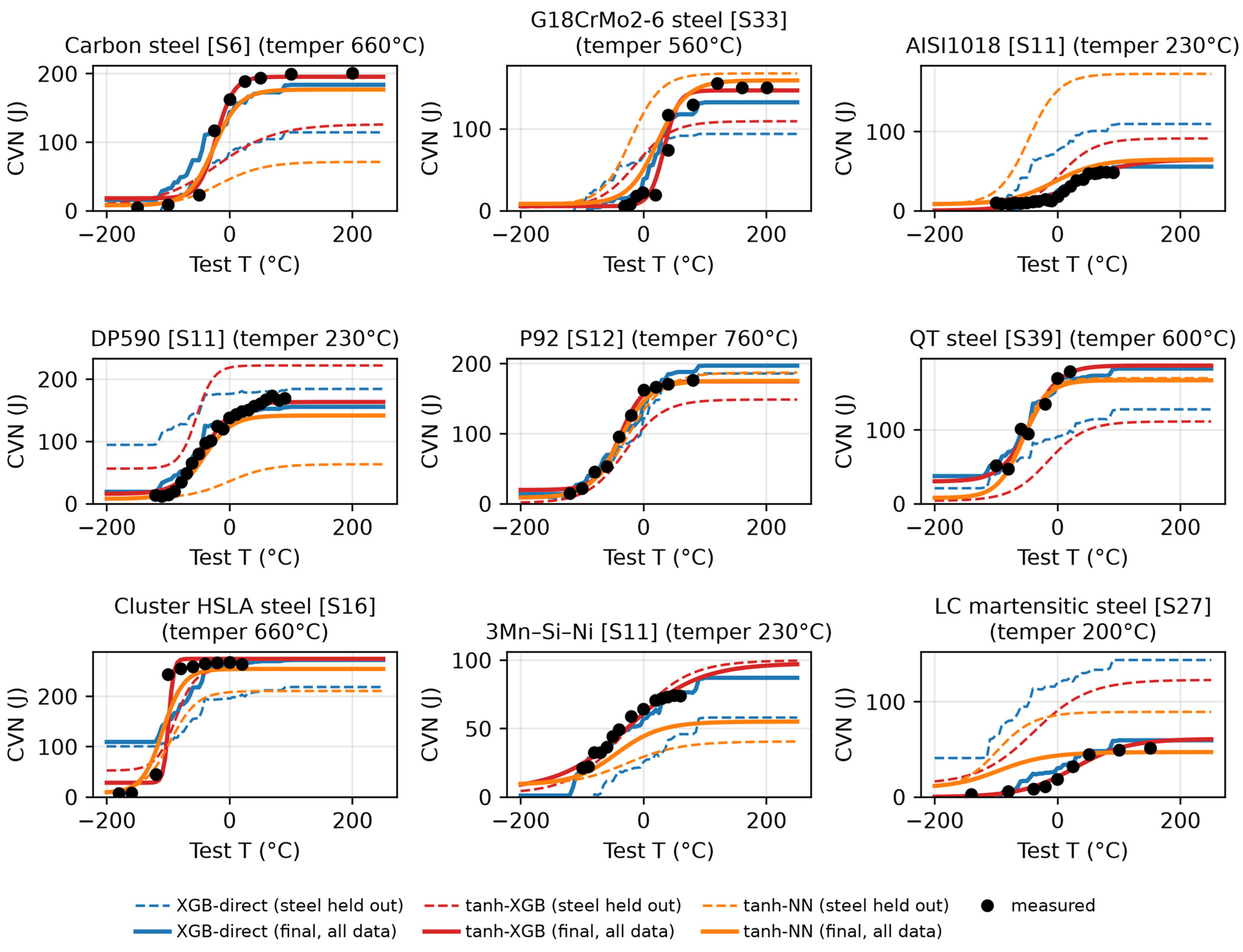
The curve-shape metrics separate the model families irrespective of accuracy. The unconstrained direct XGBoost model predicts curves with NMI = 0.06–0.08, i.e., the cumulative decrease in energy with increasing temperature amounts to several per cent of the curve height. The monotonicity constraint removes this defect completely (NMI = 0) at a cost of less than 0.03 in R2, but the curves of XGB-direct-mono remain staircases whose upper shelf is defined only by the highest test temperature in the training data (Figure 5). The direct neural network is nearly monotonic (NMI = 0.01–0.03) because it is a smooth function of the temperature input, but its curves are not sigmoids and have no defined upper shelf either. The three equation-based models return exact tanh curves. Figure 5 illustrates these differences on nine steels held out under steel grouping. The examples also show the origin of the residual error: for the P92, Q&T and 3Mn–Si–Ni steels the transition temperature is predicted within about 30 °C, whereas the upper shelf is frequently under- or overestimated by 50–100 J, and for two steels with unusually low upper shelves (AISI 1018 and the low-carbon martensitic steel) all models predict the typical shelf of their composition class. The same picture emerges when the predicted curve parameters of the equation-based models are compared directly with the parameters fitted to the 61 complete curves (Table S6). For the 31 well-resolved reference curves (Section 3.1) the mean absolute error under unseen-steel splitting is 35–41 °C in Tt and 57–64 J in USE, against standard deviations of the fitted values of 41 °C and 80 J; under unseen-condition splitting the errors are 30–37 °C and 37–50 J. For all 61 curves the unseen-steel errors are 33–41 °C and 54–63 J (standard deviations 51 °C and 100 J), and 44–53% of the predicted transition temperatures lie within ±30 °C of the fitted value, but the 30 poorly resolved reference values are themselves uncertain. The transition temperature predicted for an unseen steel is thus hardly more accurate than the mean transition temperature of the database, and the upper shelf only moderately so. A monotonic sigmoid guarantees an admissible curve shape, not an accurate transition temperature or shelf energy. When the nine steels of Figure 5 are included in the training data, the final models reproduce them with MAE = 4–50 J (XGB-direct), 5–25 J (tanh-NN) and 3–23 J (tanh-XGB; Appendix A, Figure A1), so the errors in Figure 5 arise from the extrapolation to unseen compositions and not from a lack of model capacity.
Figure 5.
Predicted DBT curves for nine steels that were completely excluded from training (unseen-steel scheme), compared with the measurements (symbols). Blue: XGB-direct; grey: XGB-direct-mono; green: two-stage; orange: tanh-NN; red: tanh-XGB. The bracketed numbers refer to the sources in Table S1.
Table 7 examines the effect of the mixed specimen geometries. Under unseen-steel splitting the pooled out-of-fold predictions for the 107 sub-size measurements are too high by 31–39 J on average for all six models (MAE 40–50 J at a median measured energy of 52 J), whereas the mean error for the 470 full-size measurements lies between −6 and +1 J: without the specimen dimensions as inputs, the models predict approximately the full-size level for sub-size specimens. For the same reason the unseen-steel R2 evaluated on the full-size measurements alone (0.19–0.43 with training on all sources, Table 7) is higher than that evaluated on all measurements (0.12–0.32, Table 6). To separate the effect of the training data from that of the evaluation population, every model was trained on the same folds with and without the measurements from sub-size and unstated-size sources and evaluated on the same held-out full-size measurements. Removing these sources from the training data changes the unseen-steel R2 of the tree models by +0.01 to +0.05 and that of the two-stage model by −0.02, and it lowers that of the networks by 0.10–0.18; under unseen-condition splitting the changes lie between −0.06 and +0.01. The increase of 0.05–0.14 that is observed when training and evaluation are both restricted to full-size sources (Table S7) therefore reflects mainly the change in the evaluation population and not cleaner training data. For the intended application, the prediction of the full-size Charpy energy of a new steel, the sub-size sources do little harm as training data for the tree models and are useful for the networks; energies predicted for sub-size specimens, however, are not reliable, and the errors quoted for all measurements include this geometry effect.
Table 7.
Effect of the specimen geometry of the training sources. Every model was trained on all measurements of the training folds (“all”) or on those from full-size-specimen sources only (“full-size”) and evaluated on the same held-out full-size measurements (470 measurements; same folds and hyper-parameters as Table 6, mean of three repetitions).
The two-stage baseline differs from the end-to-end models in the formulation, in the usable training data and in the tuning, and Table S10 separates these effects. Tuning the two-stage regressors with the procedure used for the other models raises R2 by 0.03–0.08 (to 0.60, 0.38 and 0.22 under random, unseen-condition and unseen-steel splitting). When the end-to-end models are trained only on the complete curves that the two-stage procedure can use and all models are evaluated on the held-out measurements of complete-curve conditions, tanh-XGB reaches R2 = 0.71, 0.55 and 0.41 and tanh-NN 0.77, 0.25 and −0.12, against 0.84, 0.54 and 0.33 for the tuned two-stage model (the end-to-end settings were tuned for the full database, which may disadvantage them here). With equal training data the two-stage formulation is therefore comparable with end-to-end learning on the conditions for which it is designed: more accurate under random splitting, equal to tanh-XGB under unseen-condition splitting and less accurate than tanh-XGB under unseen-steel splitting. Its low R2 in Table 6 results mainly from the 140 measurements of conditions with fewer than four test temperatures, which it cannot use for training, and to a smaller extent from the missing tuning. The advantage of the end-to-end formulation is that it accepts such measurements: trained on all data, tanh-XGB and tanh-NN reach R2 = 0.67 and 0.49 on the complete-curve measurements under unseen-condition splitting, against 0.55 and 0.25 when trained on the complete curves only.
3.3. Interpretation with SHAP
Figure 6a shows the SHAP summary of XGB-direct. The test temperature is the most influential input (mean |SHAP| = 30 J), followed by the Hollomon–Jaffe parameter (11 J), the tempering temperature (11 J), Ms (11 J), carbon (9 J), silicon (6 J), Pcm (6 J) and niobium (5 J); all other descriptors contribute less than 5 J on average. Because the test temperature dominates, the influence of composition on the shape of the curve cannot be read from this plot. The parameter-wise explanations of tanh-XGB (Figure 6b,c) resolve this. For the transition temperature, carbon dominates (mean |SHAP| = 7 °C; the dependence is monotonic, from about −10 °C at 0.05 wt.% C to +20 °C at 0.5 wt.% C), followed by PHJ (5.6 °C), the tempering temperature (5.4 °C), manganese (4 °C), Ms (3.8 °C) and copper (2.8 °C). For the upper-shelf energy the order is PHJ (13 J), carbon (13 J), tempering temperature (11 J), copper (9 J), Ms (7 J) and manganese (6 J). The dependence of USE on the tempering temperature is a step: the model attributes 20–40 J more upper-shelf energy to conditions tempered above ~600 °C than to those tempered at lower temperatures. The trends for USE are consistent with the model-free correlations of Table 5 and with metallurgical experience; for the transition temperature the model-free correlations are weak and mostly not robust (Section 3.1), so the attributions for Tt have no independent support beyond the plausible sign of the carbon effect. SHAP values describe contributions within the fitted model; given the collinearity among the descriptors (Section 3.1) and the convention of entering unreported elements as zero (Section 2.1), they do not establish independent causal effects of individual elements and are exploratory rather than mechanistic, as also noted for other small steel data sets [37]. This applies in particular to nitrogen and the other elements that most sources do not report.
Figure 6.
SHAP summary plots: (a) XGB-direct, contribution of each input to the predicted impact energy of the 604 measurements; (b) tanh-XGB, contribution of each descriptor to the predicted transition temperature Tt; (c) tanh-XGB, contribution to the predicted upper-shelf energy. Each point is one measurement (a) or one alloy/heat-treatment condition (b,c); the colour gives the descriptor value.
3.4. Prediction of the In-House Cast Steels
Figure 7 compares the DBT curves predicted from the literature database alone with the measurements of the four cast steels, and Table 8 and Table 9 list the errors. In composition the cast steels lie in the densely populated centre of the database, between the plain-carbon/HSLA and low-alloy classes; their nearest neighbours in standardised composition space are wrought quenched-and-tempered steels with 0.17–0.21 wt.% C and 1.0–1.4 wt.% Mn and the cast G18CrMo2-6 steel. The combination of a cast product form with quenching and tempering is, however, represented in the database by that single steel. Within the tested interval of −40 to 25 °C the equation-constrained neural network has the lowest error of the six models (MAE = 28 J, R2 = 0.79): it places the transition between −20 and −16 °C, inside the interval of −40 to 0 °C in which the measured energies rise most steeply (the fits of Table S15 place the mid-transition of the four steels between −24 and −4 °C), and predicts upper shelves of 172–201 J, so its energies at 25 °C fall 10–47 J below the measured 188–223 J. All other models underestimate the energy at 25 °C of all four steels by 31–101 J (MAE 44–55 J) as follows: the two-stage model and tanh-XGB reach only 113–156 J at 25 °C, although their predicted upper shelves are 141–222 J, and the direct models reach 119–157 J. The ±1 standard-deviation bands of the network ensembles (Figure 7) contain most of the tanh-NN residuals but not those of NN-direct. Table 9 resolves the errors by steel and by test temperature. The MAE of tanh-NN is 17–40 J for the individual steels; its predictions are too low at 25 and 0 °C (mean errors of −35 and −17 J) and too high at −20 and −40 °C (+21 and +23 J), i.e., the predicted transition is flatter than the measured one. The two-stage model and tanh-XGB are accurate at −40 °C (MAE 12–14 J) but fall 59–74 J short at 0 and 25 °C; the direct tree models are too high by about 60 J at −40 °C and too low by about 81 J at 25 °C, and NN-direct is too low at all four temperatures. Because the highest test temperature is 25 °C, the measurements do not establish the upper shelf of the cast steels. The agreement of tanh-NN is an agreement within the measured interval; it does not validate the complete predicted DBT curve, and in particular not the predicted upper-shelf energies. The sensitivity of the tanh-XGB prediction to the assumed heat treatment is considerable: with the as-quenched condition the error rises to 65–92 J, and tempering at 650 °C gives slightly lower errors than the actual 600 °C, so the correct specification of the heat treatment is as important as the composition.
Figure 7.
DBT curves of the four in-house cast steels (cast, 900 °C/4 h water quenched and 600 °C/4 h tempered) predicted by the six models trained on the literature database only (no information from the cast steels), compared with the measured Charpy energies (symbols). The shaded bands are ±1 standard deviation of the five ensemble members of NN-direct (cyan) and tanh-NN (orange); they show the variability among the fitted networks and are not calibrated prediction intervals.
Table 8.
Errors of the literature-trained models on the cast steels (mean over the four steels, eight measurements each) and results of the leave-one-cast-steel-out experiment (linear re-calibration and fine-tuning with the other three steels). The last two rows are baselines fitted only to the 24 measurements of the three training cast steels, without literature data; their leave-one-out errors are listed in the fine-tuned columns.
Table 9.
Errors of the literature-trained models on the cast steels by steel (MAE over the eight measurements of each steel, J) and by test temperature (MAE over the eight measurements at each temperature, J; in parentheses the mean signed error, predicted minus measured).
The low error of tanh-NN must be qualified in two respects. The first is the treatment of the elements that were not analysed (Table S11). When P, S, N and Al are set to the medians or upper quartiles of the database instead of zero, the errors of the tree-based models change little (XGB-direct 53–56 J, XGB-direct-mono 54–56 J, tanh-XGB 45–53 J and the two-stage model 39–44 J over all cases considered), whereas the networks respond strongly: tanh-NN gives 24–30 J for the median and upper-quartile cases but 49 J for the high-impurity case, and NN-direct ranges from 19 to 65 J, reaching 19–36 J whenever nitrogen is assigned a database value. With nitrogen contents typical of the database the error of NN-direct is thus comparable with that of tanh-NN, and the ranking of the two networks in the external test cannot be established without a complete chemical analysis. The coding itself was also varied (Table S14): when an element that is zero for all steels of a publication is treated as a missing value instead of a zero, in the database and for the cast steels, the grouped cross-validation R2 of the tree-based models changes by −0.02 to +0.03 and their cast-steel errors by −8 to 0 J, whereas the networks, which receive the mean of the reported values and an indicator input, become less accurate for unseen steels (R2 0.12 → 0.00 for NN-direct and 0.17 → 0.06 for tanh-NN) and for the cast steels (55 → 70 J and 28 → 35 J). The conclusions for the tree-based models therefore do not depend on the zero convention, and the sensitivity of the networks to the treatment of unreported elements is confirmed. The second is the network configuration (Table S8). The five best Optuna trials of tanh-NN, all small and strongly regularised networks (2 × 32 units, dropout 0.13–0.30) with tuning objectives within 0.02 of each other, give cast-steel errors of 26–28 J; for NN-direct the five best trials give 40–61 J. A wider tanh-NN (2 × 128 units, dropout 0.13, and weight decay 5 × 10⁻⁴) that had been selected by an earlier tuning run on a slightly different version of the database has a tuning objective of 0.32 on the present database, only 0.04 below the selected configuration, but a cast-steel error of 56 J. Configurations that cross-validation on the literature data cannot distinguish therefore differ by a factor of two in the external test.
Adapting the models with the data of three cast steels brings all of them to a similar level on the fourth (Table 8 and Figure 8): the fine-tuned networks reach MAE = 21 J (15–25 J for the individual steels) and R2 = 0.86–0.88, and the tree models 24–29 J. For orientation, the mean absolute difference between the two specimens of the cast steels is 19 J (up to 51 J at −20 °C); this is a different statistic from the MAE and is not a lower bound for it, but it indicates that the adapted models cannot be distinguished further with these data. A simple linear re-calibration of the literature prediction is as effective as fine-tuning (20–27 J for all models), which indicates that the adaptation consists mainly of lifting the level of the curve. The baselines that use the cast data alone reach the same level: 21 J for a straight line and 24 J for Equation (1) fitted to the 24 measurements of the three training steels, and 24 J for their mean at each test temperature (Table 8 and Table S12). Under this protocol the literature pre-training therefore brings no measurable benefit over fitting the in-house data directly. The fine-tuned networks and tanh-XGB are insensitive to the weight of the cast data (changes below 1 J for λ between 1 and 20), whereas the direct tree models need λ ≥ 5 (42–43 J at λ = 1; Table S12). The curve parameters of the tanh-NN fine-tuned on all four steels are Tt = −11, −15, −9 and −7 °C and USE = 212, 214, 237 and 211 J for MSN, MSNN, MSCM and MSCMN, respectively; the differences between the four steels are of the order of the specimen scatter and cannot be attributed to the individual alloying additions, and the upper-shelf values are extrapolations beyond the highest test temperature.
Figure 8.
Leave-one-cast-steel-out adaptation of tanh-NN. For each panel the model was pre-trained on the literature database (grey), re-calibrated linearly (green) or fine-tuned (red) with the measurements of the other three cast steels and evaluated on the steel shown (symbols).
4. Discussion
4.1. Direct Regression Versus Equation-Constrained Learning
In terms of point-wise accuracy under the grouped schemes, which were the tuning objective, embedding the tanh equation in the learner costs little: tanh-XGB is as accurate as XGB-direct or more so (R2 0.65 versus 0.62 under unseen-condition and 0.29 versus 0.30 under unseen-steel splitting, with a lower MAE in both), and tanh-NN is within 0.02 of NN-direct under unseen-condition splitting and not worse under unseen-steel splitting. These differences are not larger than the selection bias indicated by the nested cross-validation (−0.05 for tanh-XGB and −0.02 for XGB-direct under unseen-steel splitting, −0.05 on average over the five models; Table S5), so the data support a comparable accuracy of the two formulations and not an advantage of either. Under random splitting the picture is mixed: tanh-XGB has the lowest MAE of the tree models but an R2 depressed by a few unbounded predictions, and the small tanh-NN selected by the grouped objective interpolates less well than NN-direct (0.78 versus 0.89). The constraint pays off in three further respects. First, the predicted curves are sigmoids with a defined upper shelf, lower shelf and transition temperature, so the quantities engineers specify (a transition temperature, a 27 J or 41 J temperature, and a USE) can be read off directly. A monotonicity constraint on the test temperature removes the non-monotonicity of the direct tree model but not its staircase shape, and it leaves the upper shelf undefined beyond the range of the training temperatures (Figure 5). Second, the parameters can be interpreted separately, which turned SHAP from a description of the test-temperature effect into a ranking of composition and heat-treatment effects on Tt and USE (Figure 6). Third, the end-to-end formulation uses the 140 measurements from conditions with one to three test temperatures, which the two-stage procedure cannot exploit. This difference in usable data, together with the missing tuning, and not the two-stage formulation as such, explains why the two-stage baseline is the least accurate model under random and unseen-condition splitting: with equal training data and tuned regressors it is comparable with the end-to-end models on the complete-curve conditions (Section 3.2, Table S10). The benefit of the additional measurements is clear when other conditions of the same steel are held out, but it does not extend to unseen steels for the tree models: tanh-XGB trained with and without the sparse conditions has the same unseen-steel accuracy on the complete-curve measurements (Table S10), and removing the single-temperature conditions from the database altogether does not lower the unseen-steel accuracy of the tree models (Table S4; indicative only, because the two evaluations use different test sets). The shape guarantee has a limit: it ensures the form of the curve but not the accuracy of its parameters, which for unseen steels is low (Section 3.2). The end-to-end tanh-constrained learner thus combines the shape guarantee of the mathematical models discussed by Ahmedabadi [7] and Switzner et al. [30] with the data efficiency of a generic learner.
The choice of the learner inside the constraint matters less than the evaluation scheme. Once the networks are tuned with the same budget as the trees, the five learners that use the full database are within 0.17 of each other under unseen-condition splitting, and their differences under unseen-steel splitting (0.12–0.32) are within the repeat-to-repeat scatter (0.06–0.14). The trees are slightly better extrapolators on average, presumably because they partition the descriptor space into the steel classes of Table 2, whereas the networks interpolate smoothly between classes. The per-class errors (Table S3) show no model that is uniformly superior: the networks are much better on the high-carbon spring steels (6–19 J against 27–39 J), the trees better on the plain-carbon/HSLA class, and for the low-carbon quenched-and-tempered steels that resemble the cast steels the networks (48–49 J) are slightly better than the trees (54–55 J). The mixture of specimen geometries contributes to the errors quoted for the whole database, because the models predict the full-size level for sub-size specimens (Section 3.2); when the evaluation is restricted to full-size measurements the unseen-steel R2 of the tree models is 0.40–0.47 irrespective of whether the sub-size sources are used for training (Table 7). A model intended for full-size specimens should therefore be judged on full-size measurements, and specimen dimensions would have to be added as inputs, or the energies converted [45,46], before predictions for sub-size specimens could be used.
4.2. Limits of Extrapolation and the Value of Physics-Derived Descriptors
The drop from R2 ≈ 0.7–0.9 (random) to 0.1–0.3 (unseen steel; 0.04–0.28 in the nested procedure) quantifies how much of the apparent accuracy of Charpy-energy models comes from memorising known curves, in line with the extrapolation studies of Meredig et al. [32] and Xiong et al. [33] and with recent out-of-distribution benchmarks [34,35]. The reasons are visible in the database analysis. The upper shelf spans almost two orders of magnitude (fitted USE 5–398 J) and is determined by inclusion content, microstructure and specimen geometry, none of which is fully captured by the composition and the few processing variables that publications report; several elements are confounded with steel classes; 91 of the 169 conditions are single-temperature measurements that constrain the shelf levels only weakly; and only 31 of the 61 complete curves resolve Tt and USE well, with the median standard errors over all fits being about 10 °C and 10 J (Section 3.1). Adding descriptors that encode textbook metallurgy, the carbon equivalents, the Hollomon–Jaffe parameter and the Andrews Ms, raised the unseen-steel R2 of the tuned models by 0.03–0.13 (trees 0.16–0.21 → 0.29–0.32, networks −0.01–0.14 → 0.12–0.17; Table S2), and the Hollomon–Jaffe parameter is among the three most important SHAP features of both tree models. The gain is modest and of the order of the fold-to-fold scatter, so the descriptors are best regarded as a cheap and consistent, rather than a decisive, improvement, in line with the physical-metallurgy-guided strategy advocated for steels by Shen et al. [17] and Datta and Chattopadhyay [19]. A substantial improvement can only be expected from information that the present descriptors do not contain, such as specimen size, inclusion content or grain size, which are the most probable causes of the remaining shelf-level errors. Models restricted to one steel family or production route, often with process or microstructure variables as inputs, report much higher accuracies [21,22,23,24]; these values are not comparable with the unseen-steel results obtained here for a database that spans several steel classes, because the difficulty of the task depends on the diversity of the data and on how they are split [36,37].
4.3. External Test on the Cast Steels and Adaptation with In-House Data
The external test is the most instructive result of this work, in two respects. First, five of the six literature-trained models underestimated the room-temperature energy of the four cast steels by 31–101 J, and the small, strongly regularised tanh-NN had the lowest error within the tested temperature interval (MAE 28 J). Two causes of the underestimation can be identified. The combination of a cast product form with quenching and tempering is represented in the database by a single steel, whereas 19 of the 29 cast conditions are high-carbon steels tested at room temperature only, with energies of 2–31 J; the tree models, which partition the descriptor space, therefore associate the cast product form with low energies, while the smooth networks are less affected. In addition, the elements that were not analysed in the cast steels (P, S, N, and Al) were entered as zero, which places them at the clean end of the database; the tree-based models are insensitive to this choice, but the networks are not (Table S11). Second, the low error of tanh-NN is not robust: a wider network with a tuning objective only 0.04 lower gives 56 J (Table S8), the error rises to 49 J when high P, S and N contents are assumed, the error of NN-direct becomes comparable with that of tanh-NN when nitrogen is assigned a database value, and the ranking of the models in the external test bears little relation to the cross-validation ranking, in which the trees were the better extrapolators. A model selected by grouped cross-validation on literature data therefore does not automatically give a useful prediction for a specific new product, and an external test on independently produced material is necessary before such a model is used.
Adaptation with 24 measurements from three related cast steels reduced the error on the fourth to 21–29 J for all five adapted models, comparable in magnitude to the specimen-to-specimen scatter. This result should not be over-interpreted. The four steels differ only slightly in composition (0.18–0.24 wt.% C, 1.2–1.5 wt.% Mn, and small Ni, Cr and Mo additions) and share one heat treatment, so the leave-one-out experiment is an interpolation among near-identical steels: a linear re-calibration of the literature prediction achieves the same error as fine-tuning, and so do a straight line or a tanh curve fitted to the three training steels without any literature data (21–24 J). The experiment therefore does not isolate a benefit of the literature pre-training. What a pre-trained model could add to such a baseline is a dependence on composition and heat treatment, i.e., a prediction for an in-house steel that differs from those already tested, in the spirit of transfer learning with small data sets in materials informatics [54,55,56,57,58]; whether it does so remains to be shown with in-house steels of clearly different composition or heat treatment, for which a baseline fitted to the available in-house data is no longer adequate.
4.4. Limitations
The literature database is small and unbalanced, the heat-treatment descriptors are coarse (cooling rates are coded, prior microstructure is not recorded), specimen size and notch orientation are not available for every source, and 91 of the 169 conditions were tested at a single temperature. The sub-size and unstated-size specimens (134 measurements) were used without conversion and without specimen dimensions as inputs, so predictions for such specimens are biassed (Section 3.2), and unreported elements were entered as zero throughout. The hyper-parameters were selected on folds that overlap with the reporting folds; the nested cross-validation indicates that this inflates the unseen-steel R2 values of Table 6 by 0.05 on average, and the configuration sensitivity of the networks in the external test shows that the tuning objective does not identify a unique best network. The in-house test has several weaknesses that could not be remedied within this study: the highest test temperature of 25 °C does not establish the upper shelf, so the test covers the transition region only and the comparison of predicted and measured shelf levels is indicative; only two specimens were tested per temperature, with differences of up to 51 J between them, which is too few to determine the upper shelf and gives only a rough estimate of the transition temperature (Table S15) [53]; apart from the Brinell hardness, no microstructural or fractographic characterisation was performed; and P, S, N and Al were not analysed, and the neural networks are sensitive to the values assumed for them (Table S11). The cast specimens were machined from a 12 mm step, so only about 1 mm of the as-cast surface was removed on each side, and casting defects in the thin section may contribute to the scatter. All data, from the literature and in-house, refer to the as-heat-treated condition. The DBT curve of a component is not fixed by composition and heat treatment alone: long-term service degrades the microstructure and shifts the transition to higher temperatures, as documented for pipeline steels after decades of operation, where the transition temperature of a 17H1S steel rose from −40 to −30 °C after 31 years [59] and critically low impact toughness was found in base metal and welds after 52 years [60]. Such changes in the mechanical state during service are outside the descriptor set and the scope of the present models, which predict the curve of the material as delivered; extending them would require descriptors of the service history and data on operated material. Finally, Equation (1) assumes a symmetric transition; asymmetric functions such as the generalised logistic model used by Ahmedabadi [7] could be substituted in the same end-to-end framework without changing the methodology.
5. Conclusions
A literature database of 604 Charpy V-notch measurements on 58 steels was used to compare direct machine-learning regression of the impact energy with learners constrained by the empirical tanh equation of the DBT curve, with all models tuned under the same protocol, and the models were tested on four independently produced cast steels. The main conclusions are as follows.
- Embedding the tanh equation in the learner gives an accuracy comparable with direct regression under grouped cross-validation: the end-to-end tanh-constrained tree model and direct XGBoost regression differ by at most 0.03 in R2 when heat-treatment conditions or whole steels are held out, and the tanh-constrained network is within 0.02 of the direct network under unseen-condition splitting; these differences are not larger than the tuning-selection bias found by nested cross-validation (0.05 in R2 on average under unseen-steel splitting). The two-stage baseline that fits the equation first and regresses the parameters afterwards is less accurate under random and unseen-condition splitting (R2 = 0.58 and 0.29), mainly because it cannot use conditions tested at fewer than four temperatures; with equal training data it is comparable with end-to-end learning.
- The equation-constrained models return smooth sigmoidal curves with a defined upper shelf, lower shelf and transition temperature. A monotonicity constraint removes the non-monotonicity of direct tree regression but not its staircase shape or its undefined upper shelf. The admissible shape does not imply accurate parameters: for unseen steels the predicted transition temperature and upper-shelf energy deviate from well-resolved reference curves by 35–41 °C and 57–64 J on average.
- Extrapolation to steels absent from the training data is the limiting case for all models (R2 = 0.12–0.32; MAE 47–52 J against a standard deviation of 80 J), and the differences between the learners are within the fold-to-fold scatter. Holding out whole publications gives the same level. Part of the error stems from sub-size specimens, whose energies all models overestimate by 31–39 J; on full-size measurements the tree models reach R2 = 0.40–0.47. Physics-derived descriptors improve the unseen-steel R2 by 0.03–0.13.
- SHAP analysis of the equation-constrained tree model attributes the transition temperature mainly to carbon and tempering, and the upper-shelf energy to tempering, carbon and copper. For the upper shelf the effects of tempering and carbon agree with model-free rank correlations that remain when only well-resolved curves are used; for the transition temperature the model-free correlations are not robust, and the attributions are exploratory.
- In the external test on four in-house Q&T cast Fe–C–Mn–(Cr, Mo, Ni) steels, measured between −40 and 25 °C, the equation-constrained network had the lowest error of the six literature-trained models (MAE 28 J; other models 44–55 J). This ranking depends on network settings that cross-validation cannot resolve and on the concentrations assumed for the elements that were not analysed, and the test does not cover the upper shelf. Adapting the models with three of the cast steels brought all of them to 21–29 J on the fourth, mainly by shifting the level of the curve, but a straight line or a tanh curve fitted to the three cast steels alone was equally accurate (21–24 J), so that no benefit of the literature pre-training could be demonstrated for these closely related steels. An external test on independently produced material remains a necessary step before a literature-trained DBT-curve model is applied to a new product.
Supplementary Materials
The following supporting information can be downloaded at: https://www.mdpi.com/article/10.3390/met16111269/s1, Table S1: sources of the literature database; Table S2: effect of the physics-derived descriptors and of hyper-parameter tuning on the cross-validation results; Table S3: unseen-steel cross-validation errors by steel class; Table S4: cross-validation results without the single-temperature conditions; Table S5: nested cross-validation of the tuned models; Table S6: accuracy of the predicted curve parameters for well-resolved and poorly resolved reference curves; Table S7: cross-validation results restricted to full-size-specimen sources; Table S8: sensitivity of the external test to the network configuration; Table S9: cross-validation with whole publications held out; Table S10: two-stage and end-to-end learning with the same training data; Table S11: sensitivity of the external test to the elements not analysed in the cast steels; Table S12: baselines fitted to the cast data only and sensitivity of the fine-tuning to the weight of the cast data; Table S13: robustness of the rank correlations between descriptors and fitted curve parameters; Table S14: unreported elements coded as missing values instead of zeros; Table S15: curve parameters fitted to the eight measurements of each cast steel and their uncertainty.
Author Contributions
Conceptualization, N.S. and M.-S.K.; methodology, N.S. and S.-J.L.; software, N.S.; validation, N.S., S.-J.L. and M.-S.K.; formal analysis, N.S.; investigation, M.-S.K. and J.-W.P.; resources, M.-S.K.; data curation, N.S., J.-W.P., J.Y. and S.-J.L.; writing—original draft preparation, N.S.; writing—review and editing, N.S., J.-W.P., J.Y., S.-J.L. and M.-S.K.; visualisation, N.S.; supervision, S.-J.L. and M.-S.K.; project administration, M.-S.K.; funding acquisition, M.-S.K. All authors have read and agreed to the published version of the manuscript.
Funding
This work was partly supported by National IT Industry Promotion Agency (NIPA) grant funded by the Korea government (MSIT) (Development and Demonstration of a Manufacturing Operations System Based on Collaborative Intelligence and Physical AI, No. RS-2026-25622258) and Jeonbuk Special Self-Governing Province grant (Development of Link Arm Assembly for Korean High-Speed Train KTX Cheongryong Bogie, No. IZ250050).
Data Availability Statement
The compiled literature database (with the source list of Table S1), the in-house Charpy data, the analysis code and all model outputs are openly available in the GitHub repository https://github.com/Namhyuk516/dbtt-curve-ml (accessed on 26 October 2026), archived at Zenodo (DOI: 10.5281/zenodo.23384571; version v1.2.1: 10.5281/zenodo.24265946).
Acknowledgments
The authors gratefully acknowledge Byuck Jin Co., Ltd. (Gunsan, Republic of Korea) for their support of the project. The generative AI assistant Claude (Claude Fable 5.2; Anthropic, San Francisco, CA, USA) was used to assist with the development of the analysis code and with drafting and editing the text of this manuscript, as described in Section 2.8. All model results, numerical values, figures and interpretations were checked by the authors, who take full responsibility for the content.
Conflicts of Interest
The authors declare no conflicts of interest.
Appendix A
Figure A1 compares, for the nine steels of Figure 5, the curves predicted when the steel is excluded from training (dashed lines, as in Figure 5) with the curves of the final models trained on the complete database (solid lines). The in-sample fit of the final models over all 604 measurements is R2 = 0.89 (MAE 18.7 J) for XGB-direct, 0.86 (21.7 J) for tanh-NN and 0.97 (7.5 J) for tanh-XGB. The mean absolute errors on the nine steels are listed in Table A1.
Figure A1.
DBT curves of the nine steels of Figure 5 predicted with the steel excluded from training (dashed) and by the final models trained on all data (solid), compared with the measurements (symbols). Blue: XGB-direct; red: tanh-XGB; orange: tanh-NN.
References
- Morris, J.W., Jr. Stronger, tougher steels. Science 2008, 320, 1022–1023. [Google Scholar] [CrossRef] [Scilit] [PubMed]
- Pineau, A.; Benzerga, A.A.; Pardoen, T. Failure of metals I: Brittle and ductile fracture. Acta Mater. 2016, 107, 424–483. [Google Scholar] [CrossRef] [Scilit]
- ASTM E23-18; Standard Test Methods for Notched Bar Impact Testing of Metallic Materials. ASTM International: West Conshohocken, PA, USA, 2018.
- Oldfield, W. Curve-fitting impact test data: A statistical procedure. ASTM Stand. News 1975, 3, 24–29. [Google Scholar]
- Wallin, K. Master curve analysis of the “Euro” fracture toughness dataset. Eng. Fract. Mech. 2002, 69, 451–481. [Google Scholar] [CrossRef] [Scilit]
- Eason, E.D.; Odette, G.R.; Nanstad, R.K.; Yamamoto, T. A physically-based correlation of irradiation-induced transition temperature shifts for RPV steels. J. Nucl. Mater. 2013, 433, 240–254. [Google Scholar] [CrossRef] [Scilit]
- Ahmedabadi, P.M. Comparison of mathematical and supervised machine-learning models for ductile-to-brittle transition in bcc alloys. Mater. Res. Express 2024, 11, 076506. [Google Scholar] [CrossRef] [Scilit]
- Bhadeshia, H.K.D.H. Neural networks in materials science. ISIJ Int. 1999, 39, 966–979. [Google Scholar] [CrossRef] [Scilit]
- Bhadeshia, H.K.D.H.; MacKay, D.J.C.; Svensson, L.-E. Impact toughness of C–Mn steel arc welds—Bayesian neural network analysis. Mater. Sci. Technol. 1995, 11, 1046–1051. [Google Scholar] [CrossRef] [Scilit]
- Cottrell, G.A.; Kemp, R.; Bhadeshia, H.K.D.H.; Odette, G.R.; Yamamoto, T. Neural network analysis of Charpy transition temperature of irradiated low-activation martensitic steels. J. Nucl. Mater. 2007, 367–370, 603–609. [Google Scholar] [CrossRef] [Scilit]
- Windsor, C.G.; Cottrell, G.A.; Kemp, R. Prediction of the Charpy transition temperature in highly irradiated ferritic steels. Model. Simul. Mater. Sci. Eng. 2008, 16, 075008. [Google Scholar] [CrossRef] [Scilit]
- Mathew, J.; Parfitt, D.; Wilford, K.; Riddle, N.; Alamaniotis, M.; Chroneos, A.; Fitzpatrick, M.E. Reactor pressure vessel embrittlement: Insights from neural network modelling. J. Nucl. Mater. 2018, 502, 311–322. [Google Scholar] [CrossRef] [Scilit]
- Ferreño, D.; Serrano, M.; Kirk, M.; Sainz-Aja, J.A. Prediction of the transition-temperature shift using machine learning algorithms and the Plotter database. Metals 2022, 12, 186. [Google Scholar] [CrossRef] [Scilit]
- Agrawal, A.; Choudhary, A. Perspective: Materials informatics and big data: Realization of the “fourth paradigm” of science in materials science. APL Mater. 2016, 4, 053208. [Google Scholar] [CrossRef] [Scilit]
- Ward, L.; Agrawal, A.; Choudhary, A.; Wolverton, C. A general-purpose machine learning framework for predicting properties of inorganic materials. npj Comput. Mater. 2016, 2, 16028. [Google Scholar] [CrossRef] [Scilit]
- Guo, S.; Yu, J.; Liu, X.; Wang, C.; Jiang, Q. A predicting model for properties of steel using the industrial big data based on machine learning. Comput. Mater. Sci. 2019, 160, 95–104. [Google Scholar] [CrossRef] [Scilit]
- Shen, C.; Wang, C.; Wei, X.; Li, Y.; van der Zwaag, S.; Xu, W. Physical metallurgy-guided machine learning and artificial intelligent design of ultrahigh-strength stainless steel. Acta Mater. 2019, 179, 201–214. [Google Scholar] [CrossRef] [Scilit]
- Reddy, N.S.; Krishnaiah, J.; Hong, S.-G.; Lee, J.S. Modeling medium carbon steels by using artificial neural networks. Mater. Sci. Eng. A 2009, 508, 93–105. [Google Scholar] [CrossRef] [Scilit]
- Datta, S.; Chattopadhyay, P.P. Soft computing techniques in advancement of structural metals. Int. Mater. Rev. 2013, 58, 475–504. [Google Scholar] [CrossRef] [Scilit]
- Pattanayak, S.; Dey, S.; Chatterjee, S.; Chowdhury, S.G.; Datta, S. Computational intelligence based designing of microalloyed pipeline steel. Comput. Mater. Sci. 2015, 104, 60–68. [Google Scholar] [CrossRef] [Scilit]
- Hashimoto, Y.; Nomoto, A.; Kirk, M. Charpy V-notch energy prediction for un-irradiated reactor pressure vessel steel using the extreme gradient boost method. Metall. Mater. Trans. A 2025, 56, 3232–3243. [Google Scholar] [CrossRef] [Scilit]
- Li, H.; Jin, D.; Wu, H. Low temperature impact toughness prediction based on machine learning and microstructure verification. Steel Res. Int. 2026, 97, 5546–5556. [Google Scholar] [CrossRef] [Scilit]
- Cho, K.; Kim, G.; Kwon, S.-H.; Yim, C.-H.; Hong, D.-G. Prevention of thermal crack in steel slab using neural networks model to predict impact absorption energy. Steel Res. Int. 2024, 95, 2300732. [Google Scholar] [CrossRef] [Scilit]
- Bai, L.Q.; Ding, Z.Y.; Wang, J.L.; Xie, Z.J.; Yang, Z.N.; Shang, C.J. Predicting mechanical properties of bainitic rail steels based on microstructure digitalization and machine learning. J. Mater. Res. Technol. 2025, 35, 2136–2143. [Google Scholar] [CrossRef] [Scilit]
- Shen, C.; Mu, W.; Wang, C.; Yu, J.; Xu, W.; Hedström, P. Integrated machine learning approach for predicting low-temperature embrittlement in duplex stainless steels via ferrite hardening. J. Mater. Res. Technol. 2025, 39, 8157–8165. [Google Scholar] [CrossRef] [Scilit]
- Shang, C.; Zhu, D.; Wu, H.-H.; Bai, P.; Hou, F.; Li, J.; Wang, S.; Wu, G.; Gao, J.; Zhou, X.; et al. A quantitative relation for the ductile-brittle transition temperature in pipeline steel. Scr. Mater. 2024, 244, 116023. [Google Scholar] [CrossRef] [Scilit]
- Sahana, S.; Mahanta, B.K.; Ghosh, A.; Halder, C. Optimization of processing parameters to improve ductile-to-brittle transition of low-carbon structural steel. Mater. Manuf. Process. 2026, 41, 1619–1629. [Google Scholar] [CrossRef] [Scilit]
- Wang, P.; El-Fallah, G.M.A.M. A data-driven machine learning model for radiation-induced DBTT shifts in RAFM steels. J. Nucl. Mater. 2025, 615, 155984. [Google Scholar] [CrossRef] [Scilit]
- Jacobs, R.; Yamamoto, T.; Odette, G.R.; Morgan, D. Benchmarking and assessing models of reactor pressure vessel steel embrittlement. Mater. Des. 2026, 269, 116668. [Google Scholar] [CrossRef] [Scilit]
- Switzner, N.T.; Anderson, J.; Ali Ahmed, L.; Rosenfeld, M.; Veloo, P. Algorithms to estimate the ductile to brittle transition temperature, upper shelf energy, and their uncertainties for steel using Charpy V-notch shear area and absorbed energy data. Metals 2023, 13, 877. [Google Scholar] [CrossRef] [Scilit]
- Zhang, Y.; Ling, C. A strategy to apply machine learning to small datasets in materials science. npj Comput. Mater. 2018, 4, 25. [Google Scholar] [CrossRef] [Scilit]
- Meredig, B.; Antono, E.; Church, C.; Hutchinson, M.; Ling, J.; Paradiso, S.; Blaiszik, B.; Foster, I.; Gibbons, B.; Hattrick-Simpers, J.; et al. Can machine learning identify the next high-temperature superconductor? Examining extrapolation performance for materials discovery. Mol. Syst. Des. Eng. 2018, 3, 819–825. [Google Scholar] [CrossRef] [Scilit]
- Xiong, Z.; Cui, Y.; Liu, Z.; Zhao, Y.; Hu, M.; Hu, J. Evaluating explorative prediction power of machine learning algorithms for materials discovery using k-fold forward cross-validation. Comput. Mater. Sci. 2020, 171, 109203. [Google Scholar] [CrossRef] [Scilit]
- Omee, S.S.; Fu, N.; Dong, R.; Hu, M.; Hu, J. Structure-based out-of-distribution (OOD) materials property prediction: A benchmark study. npj Comput. Mater. 2024, 10, 144. [Google Scholar] [CrossRef] [Scilit]
- Li, K.; Rubungo, A.N.; Lei, X.; Persaud, D.; Choudhary, K.; DeCost, B.; Dieng, A.B.; Hattrick-Simpers, J. Probing out-of-distribution generalization in machine learning for materials. Commun. Mater. 2025, 6, 9. [Google Scholar] [CrossRef] [Scilit]
- Wentzien, M.; Ingber, J.; Schlötterer, J.; Friedrich, T.; Kempka, H.; Schmalzried, D.; Kunert, M. Steel microstructure analysis using transfer learning: A study on data leakage. J. Mater. Sci. 2026, 61, 13558–13580. [Google Scholar] [CrossRef] [Scilit]
- Tiwari, S.; Ahn, H.; Lee, J.; Park, N. Interpretable machine learning for mechanical property prediction of 5Cr-0.5Mo steel: SHAP explainability, multi-model comparison, and uncertainty quantification. Metals 2026, 16, 995. [Google Scholar] [CrossRef] [Scilit]
- Raissi, M.; Perdikaris, P.; Karniadakis, G.E. Physics-informed neural networks: A deep learning framework for solving forward and inverse problems involving nonlinear partial differential equations. J. Comput. Phys. 2019, 378, 686–707. [Google Scholar] [CrossRef] [Scilit]
- Karniadakis, G.E.; Kevrekidis, I.G.; Lu, L.; Perdikaris, P.; Wang, S.; Yang, L. Physics-informed machine learning. Nat. Rev. Phys. 2021, 3, 422–440. [Google Scholar] [CrossRef] [Scilit]
- Muránsky, O.; Tran, M.N.; Payten, W. On the application of PINN-style physics-regularised neural networks to high-temperature creep rupture life prediction. Int. J. Press. Vessel. Pip. 2026, 219, 105691. [Google Scholar] [CrossRef] [Scilit]
- Mei, H.; Pan, L.; Gong, C.; Zheng, X. A physics-informed neural network for creep life prediction of austenitic stainless steels in air and liquid sodium. Fatigue Fract. Eng. Mater. Struct. 2024, 47, 3584–3600. [Google Scholar] [CrossRef] [Scilit]
- Shu, C.; Zhang, S.; Ding, P.; Sun, Y.; Tao, X.; Zhu, X.; Gu, Q.; Hua, L.; Xue, S.; Yao, Z. Physics-enhanced machine learning for predicting strength of high-carbon chromium steel during thermomechanical processing and spheroidizing annealing. Mater. Des. 2025, 256, 114333. [Google Scholar] [CrossRef] [Scilit]
- Lundberg, S.M.; Lee, S.-I. A unified approach to interpreting model predictions. In Advances in Neural Information Processing Systems 30; Curran Associates: Red Hook, NY, USA, 2017; pp. 4765–4774. [Google Scholar]
- Lundberg, S.M.; Erion, G.; Chen, H.; DeGrave, A.; Prutkin, J.M.; Nair, B.; Katz, R.; Himmelfarb, J.; Bansal, N.; Lee, S.-I. From local explanations to global understanding with explainable AI for trees. Nat. Mach. Intell. 2020, 2, 56–67. [Google Scholar] [CrossRef] [Scilit] [PubMed]
- Wallin, K. Sub-sized and miniature CVN specimen conversion methodology. Int. J. Press. Vessel. Pip. 2020, 183, 104080. [Google Scholar] [CrossRef] [Scilit]
- Sreenivasulu, Y.K.; Lee, I.; Merickel, J.W.; Xu, F.; Tang, Y.; Rittenhouse, J.E.; Vakanski, A.; Song, R. Machine learning-based correlation of Charpy impact properties between sub-sized and standard-sized specimens for nuclear structural materials. Sci. Rep. 2026, 16, 16202. [Google Scholar] [CrossRef] [Scilit] [PubMed]
- Hollomon, J.H.; Jaffe, L.D. Time-temperature relations in tempering steel. Trans. AIME 1945, 162, 223–249. [Google Scholar]
- Andrews, K.W. Empirical formulae for the calculation of some transformation temperatures. J. Iron Steel Inst. 1965, 203, 721–727. [Google Scholar]
- Chen, T.; Guestrin, C. XGBoost: A scalable tree boosting system. In Proceedings of the 22nd ACM SIGKDD International Conference on Knowledge Discovery and Data Mining, San Francisco, CA, USA, 13–17 August 2016; pp. 785–794. [Google Scholar]
- Paszke, A.; Gross, S.; Massa, F.; Lerer, A.; Bradbury, J.; Chanan, G.; Killeen, T.; Lin, Z.; Gimelshein, N.; Antiga, L.; et al. PyTorch: An imperative style, high-performance deep learning library. In Advances in Neural Information Processing Systems 32; Curran Associates: Red Hook, NY, USA, 2019; pp. 8024–8035. [Google Scholar]
- Pedregosa, F.; Varoquaux, G.; Gramfort, A.; Michel, V.; Thirion, B.; Grisel, O.; Blondel, M.; Prettenhofer, P.; Weiss, R.; Dubourg, V.; et al. Scikit-learn: Machine learning in Python. J. Mach. Learn. Res. 2011, 12, 2825–2830. [Google Scholar]
- Akiba, T.; Sano, S.; Yanase, T.; Ohta, T.; Koyama, M. Optuna: A next-generation hyperparameter optimization framework. In Proceedings of the 25th ACM SIGKDD International Conference on Knowledge Discovery and Data Mining, Anchorage, AK, USA, 4–8 August 2019; pp. 2623–2631. [Google Scholar]
- Takamizawa, H.; Nishiyama, Y. Bayesian approach to model temperature dependence of Charpy absorbed energy and uncertainty evaluation of ductile-to-brittle transition temperature for reactor pressure vessel steel. J. Press. Vessel Technol. 2026, 148, 031501. [Google Scholar] [CrossRef] [Scilit]
- Jha, D.; Choudhary, K.; Tavazza, F.; Liao, W.-K.; Choudhary, A.; Campbell, C.; Agrawal, A. Enhancing materials property prediction by leveraging computational and experimental data using deep transfer learning. Nat. Commun. 2019, 10, 5316. [Google Scholar] [CrossRef] [Scilit] [PubMed]
- Yamada, H.; Liu, C.; Wu, S.; Koyama, Y.; Ju, S.; Shiomi, J.; Morikawa, J.; Yoshida, R. Predicting materials properties with little data using shotgun transfer learning. ACS Cent. Sci. 2019, 5, 1717–1730. [Google Scholar] [CrossRef] [Scilit] [PubMed]
- Zhang, L.; Shin, D.; Dimiduk, D.M.; Choi, Y.S. Leveraging transfer learning to address materials data scarcity: A case study on predicting hardness in additively manufactured high-entropy alloys. npj Comput. Mater. 2026, 12, 355. [Google Scholar] [CrossRef] [Scilit]
- Yin, Q.; Liu, Y.; Zhao, H.; Wang, J.; Zhang, S.; Fan, Y.; Dong, X.; Song, Y.; Guo, C. Accelerated Cu-Ti alloy design under data scarcity through fine-tuned transfer learning. Mater. Des. 2025, 260, 115055. [Google Scholar] [CrossRef] [Scilit]
- Zong, B.; Li, J.; Yuan, T.; Wang, J.; Yuan, R. Recent progress on machine learning with limited materials data: Using tools from data science and domain knowledge. J. Mater. 2025, 11, 100916. [Google Scholar] [CrossRef] [Scilit]
- Krechkovska, H.; Kulyk, V.; Vira, V.; Student, O. Influence of long-term operation of the 17H1S steel on the main gas pipeline on the change of the mechanical properties. Procedia Struct. Integr. 2022, 36, 334–341. [Google Scholar] [CrossRef] [Scilit]
- Zvirko, O.I.; Kryzhanivskyi, Y.I.; Hredil, M.I.; Nykyforchyn, H.M.; Tsyrulnyk, O.T. Susceptibility of a welded joint of an operated gas distribution pipeline to brittle fracture. Mater. Sci. 2025, 61, 59–65. [Google Scholar] [CrossRef] [Scilit]
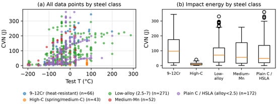
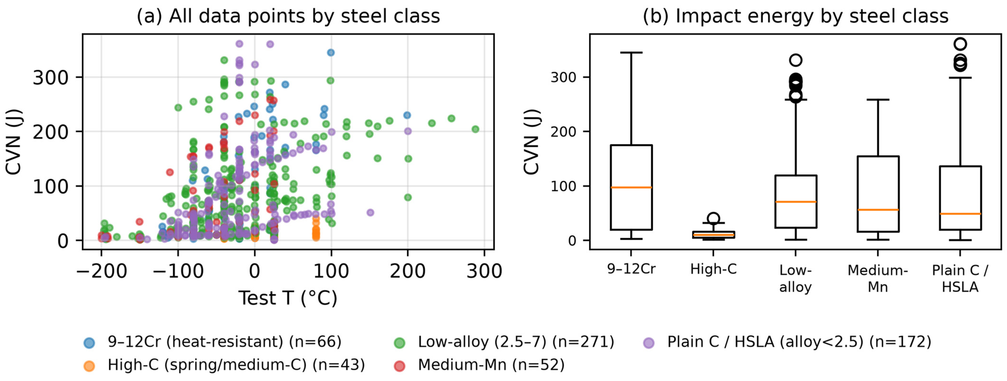
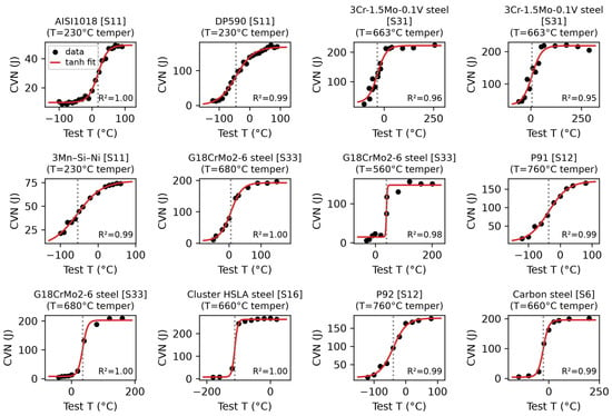
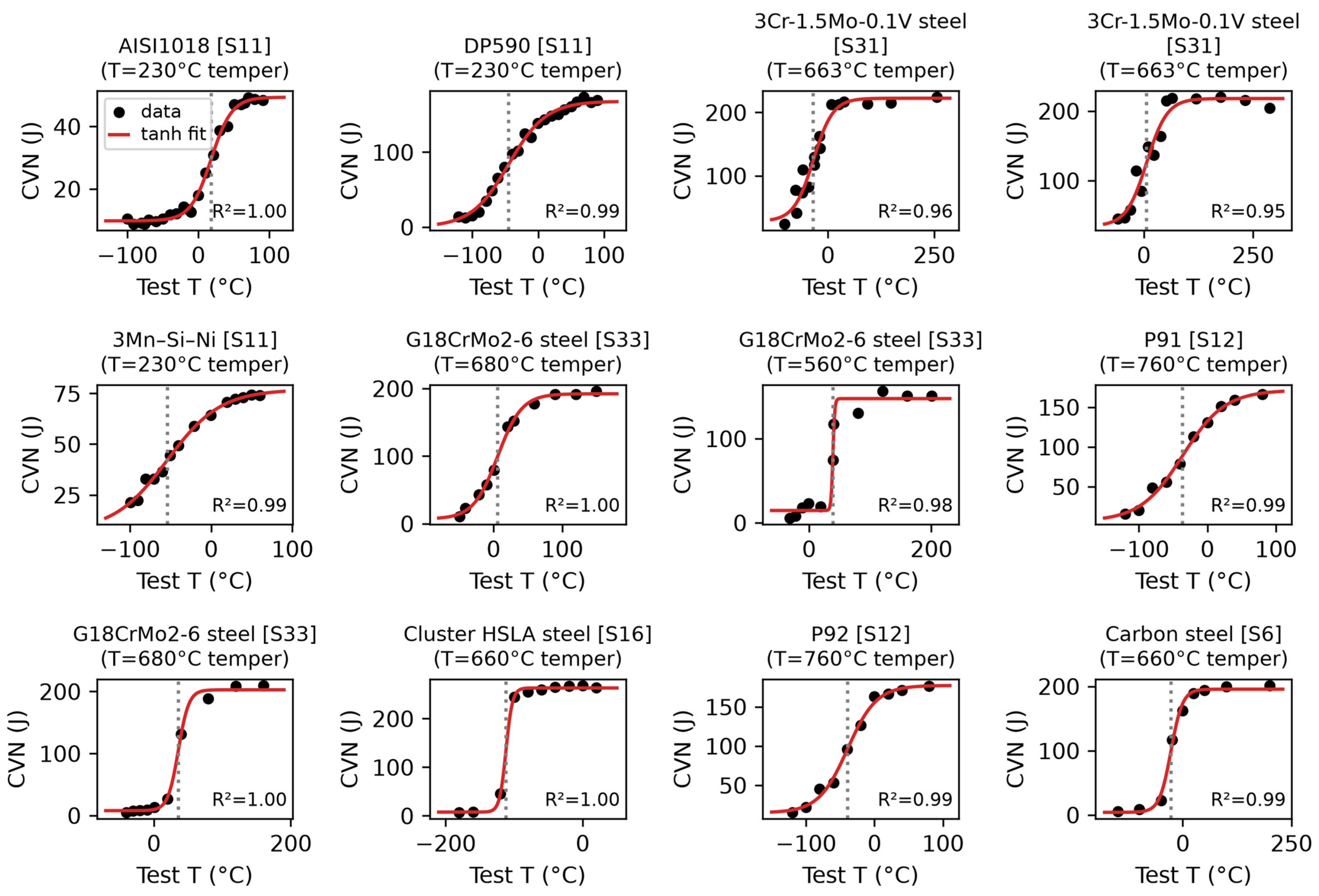
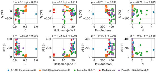
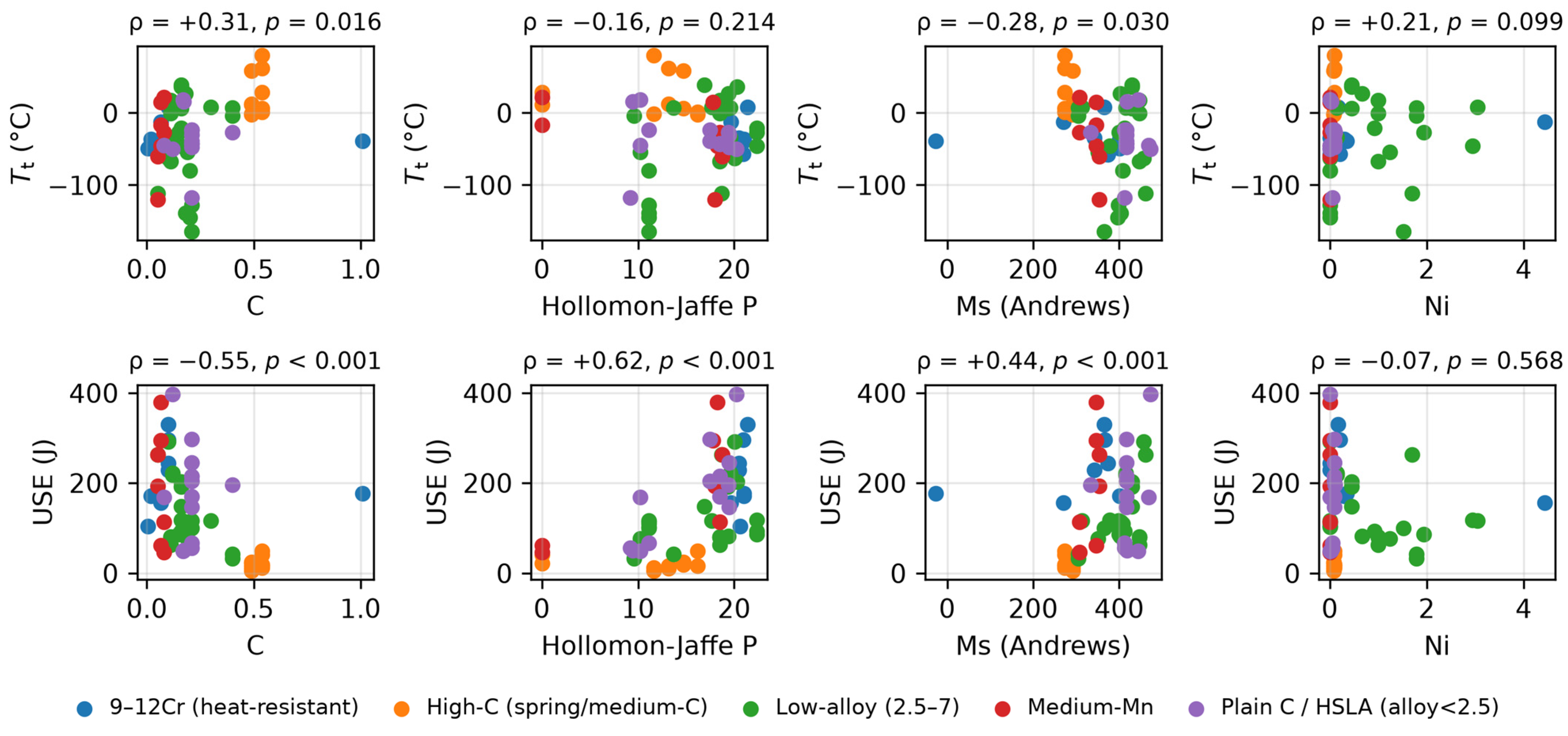
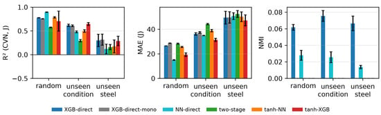
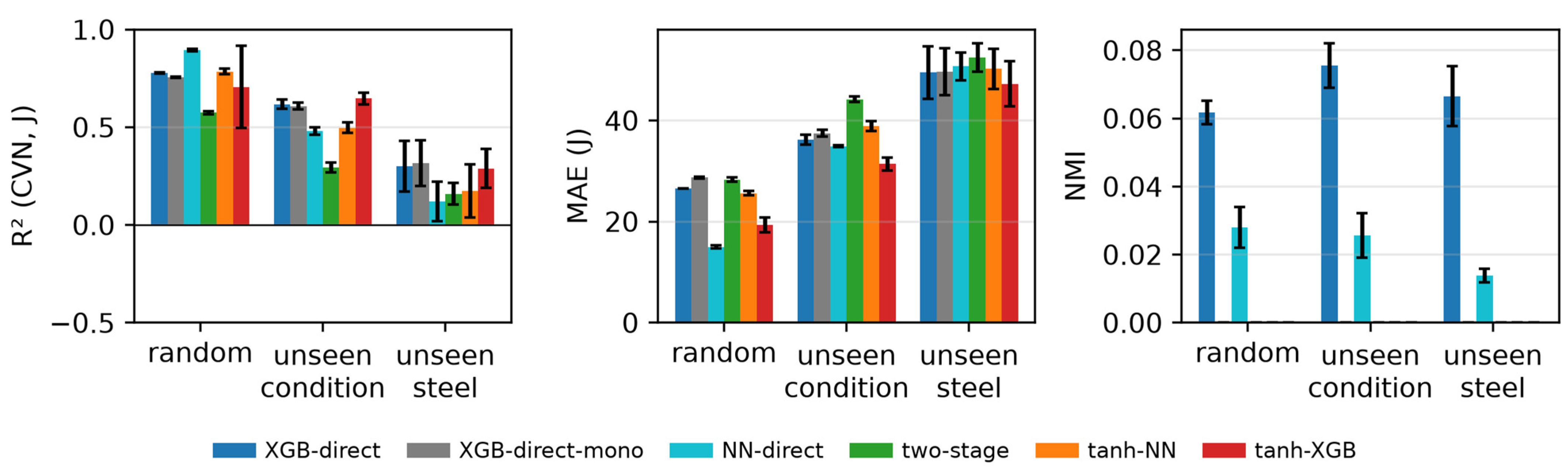
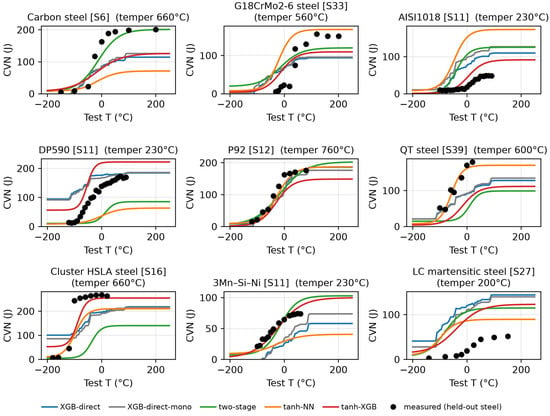
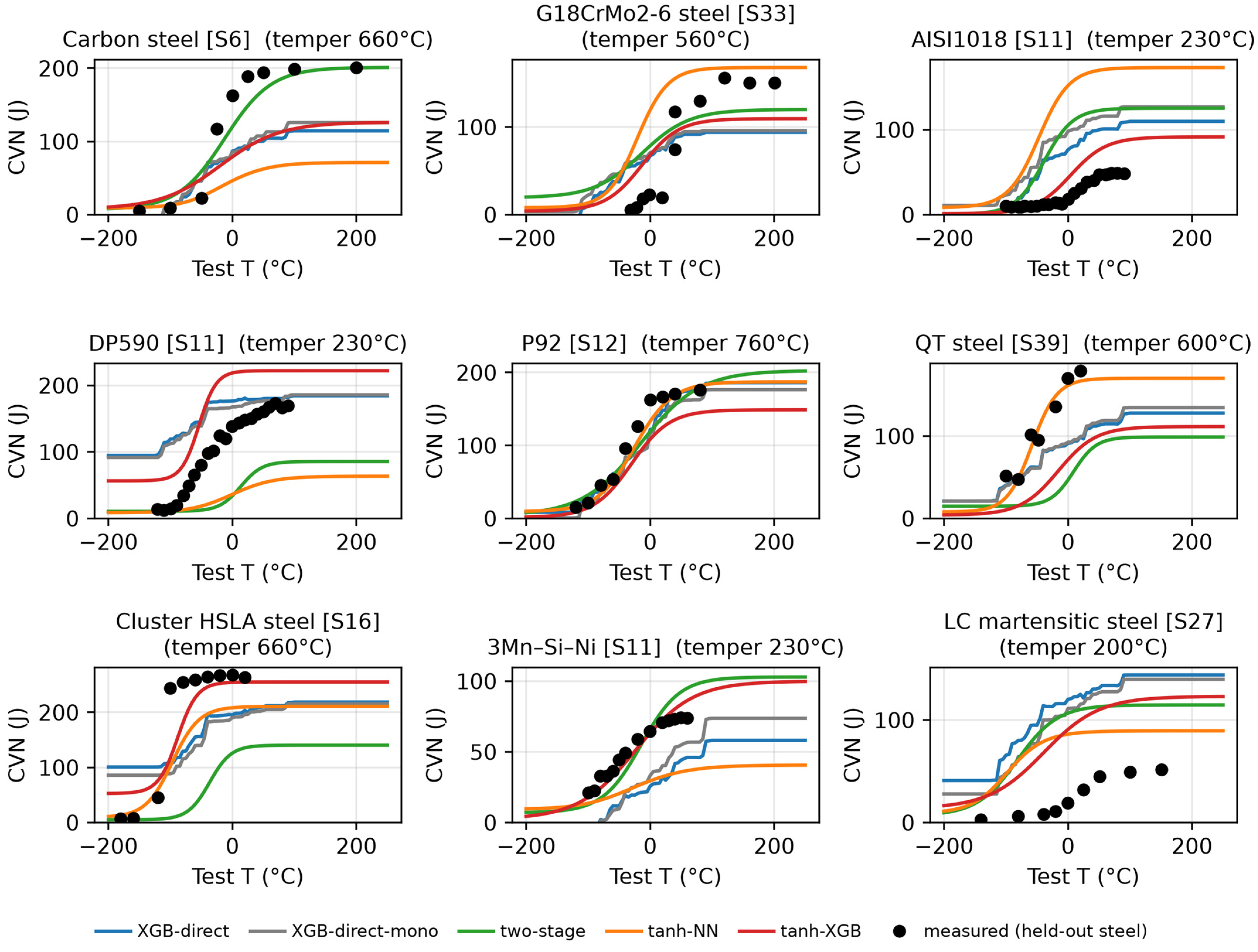
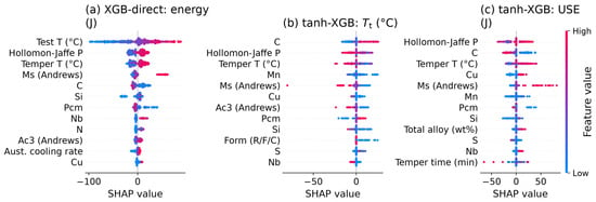
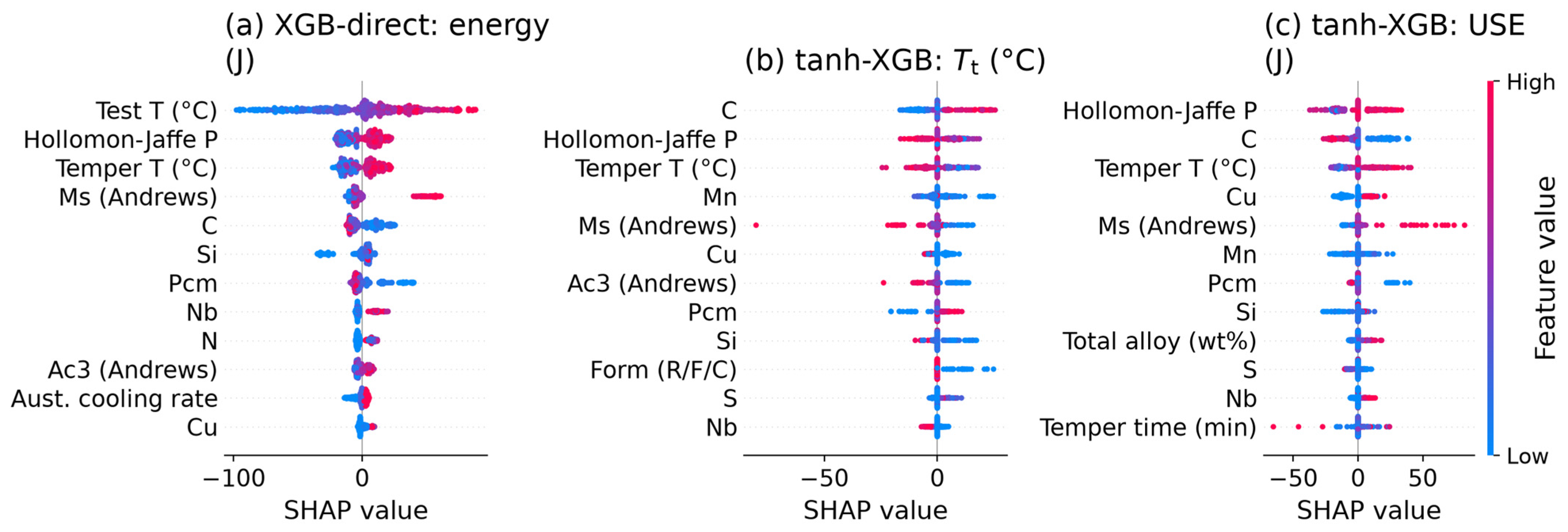
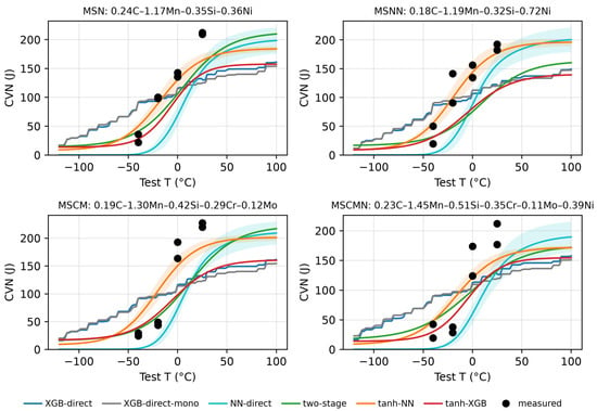
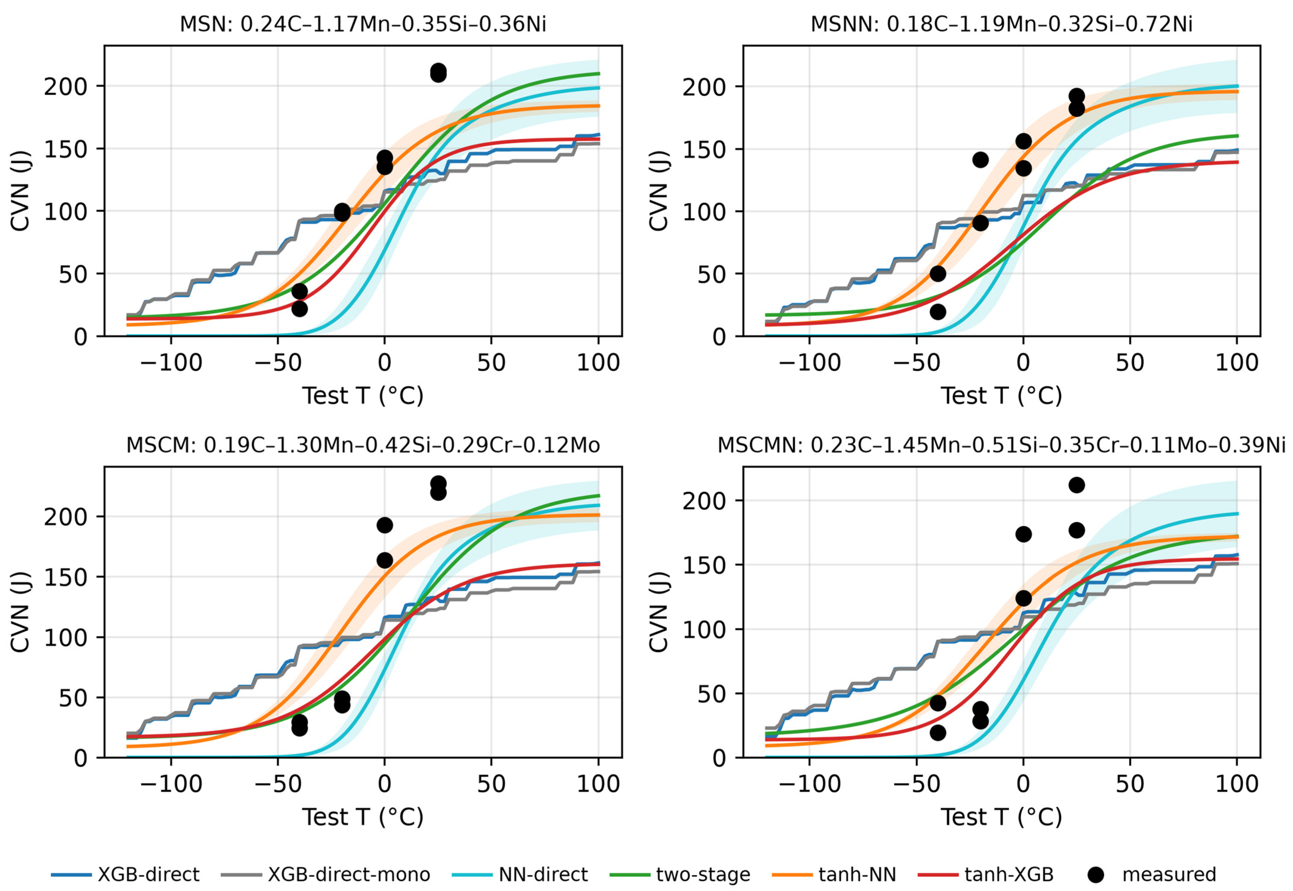
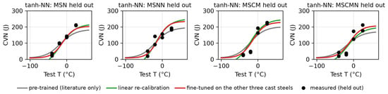
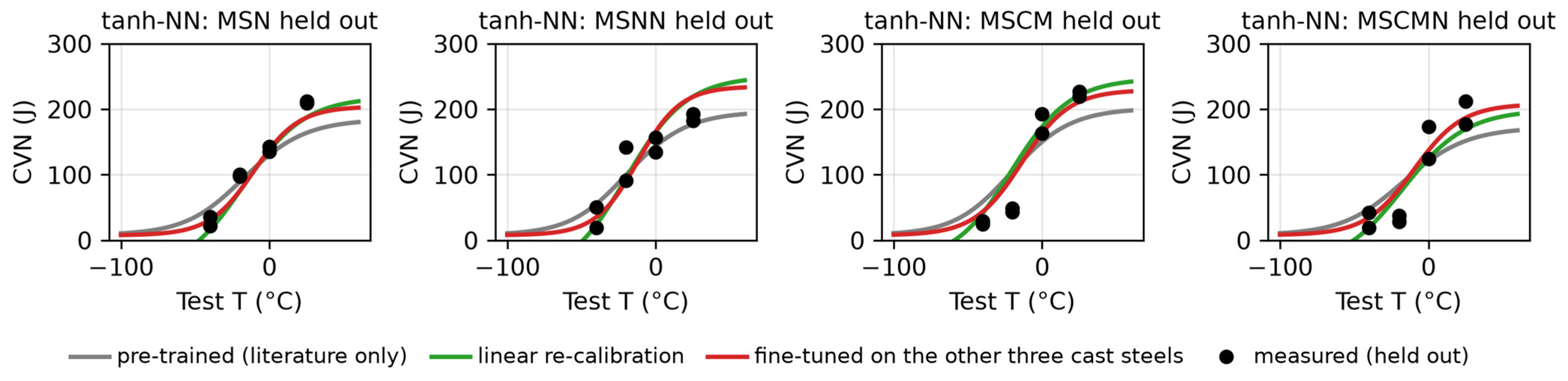

Disclaimer/Publisher’s Note: The statements, opinions and data contained in all publications are solely those of the individual author(s) and contributor(s) and not of MDPI and/or the editor(s). MDPI and/or the editor(s) disclaim responsibility for any injury to people or property resulting from any ideas, methods, instructions or products referred to in the content. |
© 2026 by the authors. Licensee MDPI, Basel, Switzerland. This article is an open access article distributed under the terms and conditions of the Creative Commons Attribution (CC BY) license.