Wavelet-Based Scalogram Analysis of Surface Texture and Technological Heredity in Turning and Burnishing

Abstract

Machined surfaces can retain features from preceding operations, complicating the identification of their processing history. This study develops a wavelet-based method to identify routes and quantify technological heredity (process-history effects) from surface profiles. Profiles from 40-mm-diameter shafts made of 12Kh18N10T stainless steel (broadly comparable to AISI 321) were analyzed using the continuous wavelet transform with a complex Morlet wavelet. Scalograms were partitioned into nine Taguchi L9 regions and described by five features: peak intensity, relative peak intensity, relative spatial and period coordinates of the peak, and relative high-energy area $S_{75}$. Robustness was evaluated using the Taguchi signal-to-noise metric at artificial noise levels up to 50%. Discrimination was assessed using principal component analysis (PCA), Fisher scores, and nearest-centroid and k-nearest-neighbor classification. Two-way analysis of variance (ANOVA) quantified technological heredity; the unexplained variance ratio $({\mathrm{SS}}_{IJ}+{\mathrm{SS}}_{\mathrm{err}})/{\mathrm{SS}}_{\mathrm{tot}}$ represented the variability not explained by the main effects of period and spatial position. Classification performance depended on the route group: for Group 2, profile-level 1-nearest-neighbor validation gave 7/18 correct classifications from the scalogram descriptors and 18/18 from $R_a$, $R_q$, and $R_z$. Routes involving burnishing exhibited lower unexplained variance and more compact PCA clusters, whereas routes combining rough and finish turning showed stronger heredity signatures and more complex scalogram structures. The framework therefore provides complementary scale-resolved information and a descriptive assessment of process-history-related variability; general route identification requires further validation. The proposed scalogram descriptors are intended to complement, rather than replace, conventional roughness parameters such as $R_a$, $R_z$, and $R_q$, by providing additional information on the scale- and position-resolved structure of the machined surface.

1. Introduction

Surface texture is formed by tool geometry, process parameters, and machining sequence. In multistage machining, finished surfaces may retain signatures of finishing operations as well as traces of earlier stages. This transfer of geometric features is described in the machining literature as technological heredity, i.e., a process-history effect [1,2]. During sequential manufacturing operations, microstructural and geometrical irregularities induced during rough cutting can propagate through subsequent passes, fundamentally dictating the operational performance, contact stiffness, wear resistance, and fatigue life of the finished components [3,4]. Accurately tracking and controlling this inheritance is critical for optimizing high-reliability components subjected to severe mechanical and thermal environments.

Conventional roughness parameters such as $R_a$ and $R_z$ are standardized and useful for quality control, but they may be insufficient for distinguishing machining routes when different operations produce similar scalar roughness values. In such cases, detailed surface-profile features, including local periodicity, amplitude concentration, and spatial modulation, provide additional information about manufacturing history [5]. Recent wavelet-based studies have likewise shown that multiscale descriptors can reveal process-dependent surface features that are not represented by a single roughness value and can support automated surface-texture classification [6,7,8]. For example, Shumetova and Mel’nikov demonstrated that continuous wavelet transform (CWT) scalograms can effectively decompose the multi-layered topography of machined surfaces to identify characteristic zones and trace technological inheritance where standardized profile parameters remain ambiguous [9].

Mechanical surface treatments such as ball burnishing and burnishing with a fixed indenter modify both the surface texture and the energy-force conditions at the tool–workpiece contact. Previous studies by Bobrovskij, Khaimovich, and co-authors showed that initial surface texture, friction conditions, and indenter loading govern roughness formation and burnishing-process stability [10,11]. Recent surface-characterization experiments further confirm that the texture produced by the preceding turning operation affects the surface obtained after burnishing [12,13]. Recent comprehensive investigations by Maximov et al. on chromium–nickel austenitic stainless steels demonstrated that surface integrity, residual stress distribution, and fatigue resistance after diamond burnishing are profoundly influenced by the kinematic conditions and feed marks established during earlier turning passes [14,15]. Furthermore, finite element and experimental modeling by Chodór et al. highlighted that burnishing induces severe localized elastoplastic deformation that flattens asperity summits and redistributes material into valleys, thereby transforming the periodic harmonic signatures of turned profiles [16].

Time–frequency analysis is therefore preferable to purely spectral methods. While Fourier analysis describes global frequency content, wavelet analysis can simultaneously localize features in scale and coordinate, making it suitable for surface signals with nonstationary or spatially heterogeneous structure [17,18,19,20]. Recent applications of the continuous wavelet transform (CWT) to turned and milled surfaces demonstrate that Morlet-based profile analysis and scale-resolved surface descriptors can identify localized disturbances and machining-dependent multiscale structures [21,22].

For multistage manufacturing, quantitative heredity coefficients based on changes in waviness have demonstrated that the signatures generated at one stage may persist, weaken, or be transformed during subsequent operations [1]. In parallel, time–frequency representations derived from the CWT have been used as discriminative inputs for automated roughness classification [23]. These strands of research generally treat multiscale characterization, route classification, and process-history effects separately; the present work combines them in a single interpretable framework.

It should be emphasized that the objective of this study is not to replace standardized scalar roughness parameters, such as $R_a$, $R_q$, or $R_z$, which remain essential and well-established descriptors of surface quality in industrial practice. Rather, the proposed scalogram-based descriptors are intended to complement these parameters by capturing how wavelet energy associated with characteristic periodicities is distributed and localized along the measured profile—information that a single scalar value cannot represent. The novelty of the present work lies in combining this complementary multiscale representation with a structured period–coordinate partition, discriminative analysis, and variance decomposition into a single interpretable framework for machining-route identification and residual-variability assessment in multistage turning–burnishing chains.

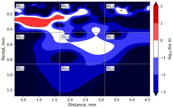
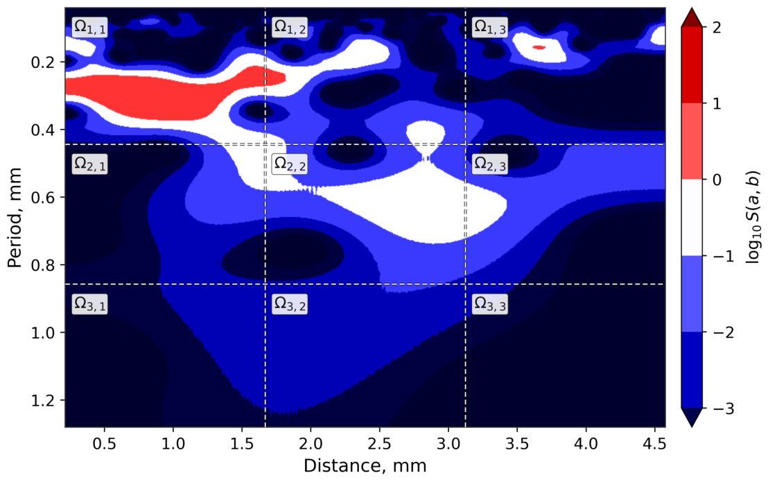
The objective of this work is to develop a scalogram-based framework that can (i) identify machining routes from surface profiles and (ii) quantify residual multiscale variability associated with technological heredity by combining Morlet wavelet analysis, Taguchi L9 partitioning, discriminative analysis, and variance decomposition using analysis of variance (ANOVA) (Figure 1).

Figure 1. Example of a scalogram obtained from the continuous wavelet transform using a Morlet wavelet and partitioned into nine Taguchi L9 regions.

2. Materials and Methods

2.1. Workpieces and Machining Routes

The experiments were conducted on 40-mm-diameter cylindrical shafts made of Russian-grade 12Kh18N10T austenitic stainless steel. Its closest commonly used international counterparts are AISI 321 (UNS S32100) and EN X6CrNiTi18-10 (material no. 1.4541); this correspondence is approximate because the requirements of the respective standards are not identical. This material features an austenitic face-centered cubic matrix stabilized with titanium (≈17–19% Cr, 9–11% Ni, 0.5–0.8% Ti, balance Fe). It exhibits high ductility, moderate yield strength (${\sigma }_{0.2}\approx 205$ MPa), ultimate tensile strength (${\sigma }_b\approx 520$ MPa), and initial hardness of approximately 160 HB. Because of its pronounced strain-hardening tendency and low thermal conductivity, 12Kh18N10T is particularly sensitive to severe surface deformation and thermo-mechanical tool–workpiece interaction during machining and surface plastic deformation [14,15]. Two groups of machining routes were considered: Group 1 for route classification and Group 2 for the analysis of technological heredity.

Group 1 included four routes: route 1-1 (rough turning); route 1-2 (rough turning followed by burnishing); route 1-3 (rough turning followed by finish turning); and route 1-4 (rough turning followed by finish turning and burnishing). Group 2 included six routes: route 2-1 (rough turning); route 2-2 (rough turning followed by ball burnishing); route 2-3 (rough turning followed by ball burnishing and subsequent burnishing); route 2-4 (rough turning followed by finish turning); route 2-5 (rough turning followed by finish turning and ball burnishing); and route 2-6 (rough turning followed by finish turning, ball burnishing, and subsequent burnishing).

In this paper, burnishing is defined as a fixed indenter sliding over a rotating workpiece under controlled normal force, whereas ball burnishing uses a bearing steel ball rolling over the workpiece with a prescribed radial indentation.

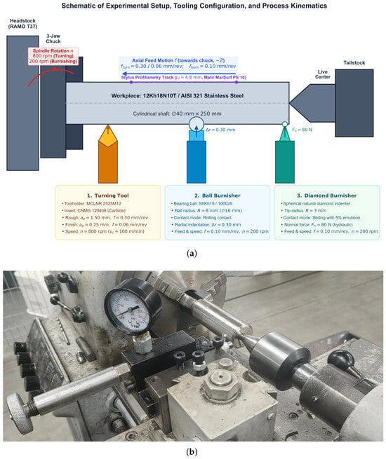
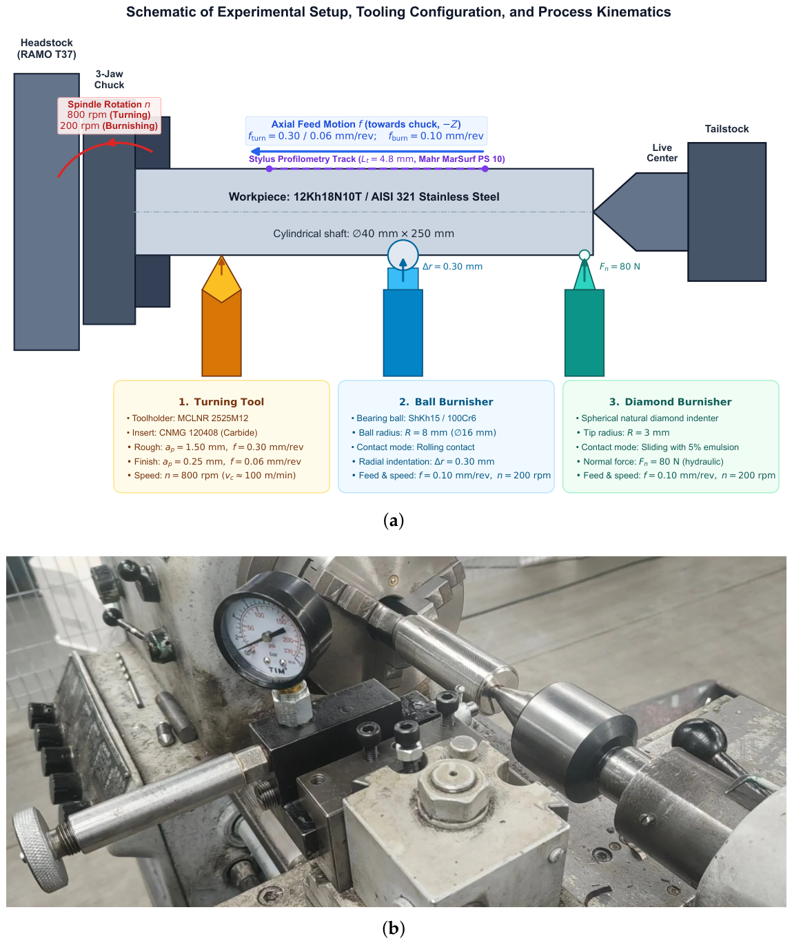
All turning and burnishing operations were performed on a RAMO T37 center lathe (RAMO, Niort, France). The machine and the burnishing setup are shown in Figure 2, and the machining parameters and tools used in the experiments are summarized in Table 1. The workpiece was rigidly clamped in a three-jaw chuck with support from a live tailstock center to ensure high structural rigidity and minimize vibration. All operations were conducted with flood application of a 5% water-miscible emulsion coolant.

Figure 2. Experimental setup, tooling configuration, and burnishing arrangement: (a) Technical schematic showing workpiece mounting (12Kh18N10T stainless steel cylindrical shaft, $⌀40\times 250$ mm, supported between 3-jaw chuck and live center), spindle rotation n, axial feed motion f (towards headstock, $-Z$), tool arrangements for rough and finish turning (CNMG 120408), ball burnishing ($⌀16$ mm bearing ball, radial indentation $\Delta r=0.30$ mm), and diamond sliding burnishing (spherical diamond indenter $R=3$ mm, normal force $F_n=80$ N), along with the stylus profilometry measurement track ($L_t=4.8$ mm); (b) Photograph of the experimental burnishing setup on the RAMO T37 lathe showing the pressure-controlled burnishing device with a manometer mounted in the tool post, rotating workpiece, and tailstock live center.

Table 1. Machining equipment, tools, and nominal process parameters used in the experiments.

Operation	Process Conditions	Tool
Rough turning	Spindle speed: 800 rpm; depth of cut: 1.50 mm; feed: 0.30 mm/rev	MCLNR2525M12 toolholder with CNMG 120408 indexable insert (Sandvik Coromant, Sandviken, Sweden) designed for machining stainless steel
Finish turning	Spindle speed: 800 rpm; depth of cut: 0.25 mm; feed: 0.06 mm/rev	MCLNR2525M12 toolholder with CNMG 120408 indexable insert (Sandvik Coromant, Sandviken, Sweden) designed for machining stainless steel
Burnishing	Spindle speed: 200 rpm; normal force: 80 N; feed: 0.10 mm/rev	Spherical diamond indenter with a tip radius of 3 mm (JSC AlmazInstrument, Moscow, Russia)
Ball burnishing	Spindle speed: 200 rpm; radial tool indentation: 0.30 mm; feed: 0.10 mm/rev	ShKh15 bearing steel ball (broadly comparable to SAE 52100 and EN 100Cr6, material no. 1.3505) with a radius of 8 mm

For ball burnishing, a radial tool indentation of 0.30 mm was set using the RAMO T37 cross-slide vernier scale. For burnishing, a normal force of 80 N was determined from the hydraulic pressure-gauge reading using the tool-specific pressure-to-force relationship.

2.2. Continuous Wavelet Transform and Scalogram Definition

The measured surface profile $h\left(x\right)$ was treated as a one-dimensional signal and processed using the CWT. The CWT is defined as

$$W(a,b)={\int }_{-\infty }^{+\infty }h\left(x\right){\psi }_{a,b}^{*}\left(x\right)\mathrm{d}x,$$

(1)

where $a>0$ is the scale parameter, b is the coordinate shift, and ${\psi }_{a,b}\left(x\right)$ is the scaled and shifted analyzing wavelet [18,20].

For the Morlet wavelet, the analyzing wavelet was implemented using the PyWavelets complex Morlet parameterization

$$\psi \left(x\right)={\displaystyle \frac{1}{\sqrt{\pi B}}}exp\left(-{\displaystyle \frac{x^2}{B}}\right)exp\left(\mathrm{i}2\pi Cx\right),$$

(2)

and the scaled and shifted version was

$${\psi }_{a,b}\left(x\right)={\displaystyle \frac{1}{\sqrt{a}}}\psi \left({\displaystyle \frac{x-b}{a}}\right).$$

(3)

The scalogram was defined as the local energy of the wavelet representation,

$$S(a,b)={\left|W(a,b)\right|}^2.$$

(4)

The continuous wavelet transform was evaluated using PyWavelets 1.4.1 [24] with the complex Morlet wavelet cmor1.5-1.0, where $B=1.5$ is the bandwidth parameter and $C=1.0$ is the center frequency in cycles per sample. The corresponding angular carrier frequency is ${\omega }_0=2\pi C=2\pi \approx 6.283$ rad per sample. Each profile was interpolated to $\Delta x=1.0\mathsf{\mu }\mathrm{m}$ and standardized to zero mean and unit standard deviation. The CWT was evaluated by FFT convolution at $N=64$ linearly spaced scales, $a_n=4+n(124/63)$ for $n=0,\dots ,63$. PyWavelets defines the equivalent frequency as $f\left(a\right)=C/(a\Delta x)$ and hence $T\left(a\right)=a\Delta x/C$. Because $C=1.0$ and $\Delta x=1.0\mathsf{\mu }\mathrm{m}$, the scale array corresponds directly to periods from 4.0 to 128.0 $\mathsf{\mu }\mathrm{m}$. No user-defined $L_1$ rescaling or additional admissibility correction was applied; the coefficients were used with the normalization implemented by PyWavelets.

This representation makes it possible to analyze the surface profile simultaneously in terms of period (scale) and spatial coordinate, which is especially important for nonuniform roughness patterns and multistage machining signatures [18,20].

2.3. Taguchi L9 Partition and Local Feature Extraction

To analyze the scalogram in a structured way, the period–coordinate domain was divided into nine rectangular regions according to a Taguchi L9 design with two factors and three levels: factor I for period and factor J for spatial coordinate. This partition makes it possible to separate the effect of characteristic wavelengths from the effect of spatial localization along the surface profile [25,26].

The $3\times 3$ resolution was selected as a compromise between physical interpretability and statistical stability. A finer partition would provide better scale and spatial localization but would proportionally increase the dimensionality of the feature vector relative to the limited number of replicated profiles (three per route), amplifying the risk of overfitting in the discriminative analysis. A coarser partition would reduce the ability to separate short-, intermediate-, and long-period components. The sensitivity of the results to this choice was evaluated by comparing the $3\times 3$ partition against a coarser $2\times 2$ aggregation (Section 2.7 and Section 3.5).

In each cell ${\mathrm{\Omega }}_{IJ}$, five local descriptors were calculated: $I_{max}$, $I_{mean}$, $x_{peak}^{rel}$, $perio{d}_{peak}^{rel}$, and $S_{75}$ (Equations (5)–(10)). The peak intensity was defined as

$$I_{\max }^{I,J}=\underset{(a,b)\in {\mathrm{\Omega }}_{IJ}}{\max }S(a,b).$$

(5)

The mean intensity in the same cell was defined as

$$I_{\mathrm{mean}}^{I,J}={\displaystyle \frac{1}{N_{IJ}}}\sum _{(a,b)\in {\mathrm{\Omega }}_{IJ}}S(a,b),$$

(6)

where $N_{IJ}$ is the number of scalogram samples in cell ${\mathrm{\Omega }}_{IJ}$.

The relative coordinates of the peak intensity were computed as

$$x_{\mathrm{peak}}^{I,J}={\displaystyle \frac{b_{\mathrm{peak}}-b_{min}^J}{b_{\max }^J-b_{min}^J}},{\mathrm{period}}_{\mathrm{peak}}^{I,J}={\displaystyle \frac{T_{\mathrm{peak}}-T_{min}^I}{T_{\max }^I-T_{min}^I}}.$$

(7)

The 64 scale samples were divided by fixed array indices into groups of 21, 21, and 22 samples. Their included period centers were $I_1=4.00$–$43.37\mathsf{\mu }\mathrm{m}$, $I_2=45.33$–$84.70\mathsf{\mu }\mathrm{m}$, and $I_3=86.67$–$128.00\mathsf{\mu }\mathrm{m}$. The 4800 coordinate samples were divided into three groups of 1600 points: $J_1=0$–$1599\mathsf{\mu }\mathrm{m}$, $J_2=1600$–$3199\mathsf{\mu }\mathrm{m}$, and $J_3=3200$–$4799\mathsf{\mu }\mathrm{m}$. In Equation (7), $T_{min}^I$, $T_{\max }^I$, $b_{min}^J$, and $b_{\max }^J$ are the first and last sampled coordinates included in the corresponding cell. The same fixed index boundaries were used for every profile.

Each surface profile was therefore represented by 45 features (9 cells × 5 descriptors), which formed the basis for classification and heredity analysis.

The threshold $0.75I_{max}^{I,J}$ defines $S_{75}^{I,J}$ as an operational descriptor of the relative spatial occupancy of the high-energy core of a cell, rather than a physically fixed constant. It quantifies whether the strongest local scalogram feature in a cell is concentrated in a small region or distributed over a wider area, providing information about the spatial compactness of the corresponding surface component.

The physical meaning of the five local descriptors can be summarized as follows. $I_{\max }^{I,J}$ represents the strongest localized wavelet-energy event within a given period–coordinate cell and is associated with the most pronounced profile component at that scale and location. $I_{\mathrm{mean}}^{I,J}$ represents the average energy level within the same cell, and the ratio $I_{\max }^{I,J}/I_{\mathrm{mean}}^{I,J}$ represents the degree of energy concentration: high values correspond to isolated, sharply localized features, whereas low values indicate a more uniformly distributed texture. $x_{\mathrm{peak}}^{I,J}$ and ${\mathrm{period}}_{\mathrm{peak}}^{I,J}$ identify the relative position of the dominant local component within the coordinate and period ranges of the cell, respectively. Finally, $S_{75}^{I,J}$ estimates the spatial extent of the high-energy core. Unlike $R_a$ or $R_z$, which reduce an entire profile to a single amplitude-based value, these descriptors retain information about where and how strongly specific periodic components occur along the profile, offering a complementary characterization of machining-induced surface structure.

The relative peak intensity was calculated as

$${\displaystyle \frac{I_{\max }^{I,J}}{I_{\mathrm{mean}}^{I,J}}}.$$

(8)

The relative high-energy area was defined by the threshold condition

$$S(a,b)\ge 0.75I_{\max }^{I,J},$$

(9)

and the corresponding relative area was

$$S_{75}^{I,J}={\displaystyle \frac{N_{75}^{I,J}}{N_{IJ}}},$$

(10)

where $N_{75}^{I,J}$ is the number of scalogram samples satisfying Equation (9). Each surface profile was therefore represented by 45 features (9 cells × 5 descriptors), which formed the basis for classification and heredity analysis.

2.4. Robustness Assessment Using the Taguchi Signal-to-Noise Ratio

To evaluate descriptor sensitivity, zero-mean Gaussian perturbations were added directly to the measured surface profile $h\left(x\right)$ prior to wavelet processing. The noise standard deviation was defined as a fraction of the peak-to-peak amplitude of the measured profile, ${\sigma }_{\mathrm{noise}}=k·\max \left|h\left(x\right)\right|$, $k\in \{0.10,0.20,0.50\}$, so that the reported noise levels of 10%, 20%, and 50% correspond to amplitude-based perturbation levels rather than to a calibrated model of Mahr MarSurf PS 10 measurement uncertainty. The 10% and 20% levels represent moderate sensitivity tests, whereas the 50% level is an intentionally severe perturbation used to examine the resistance of the descriptors to strong signal degradation. The scalogram and the local descriptors were then recomputed from each noisy realization, and robustness was quantified using the Taguchi signal-to-noise ratio (Equation (11)).

For each descriptor, robustness was quantified using the Taguchi “smaller-the-better” signal-to-noise ratio, here denoted ETA and expressed in decibels (dB) [25,27]:

$$\mathrm{ETA}=-10{log}_{10}\left[{\displaystyle \frac{1}{n}}{\displaystyle \sum _{k=1}^n}{\left({\displaystyle \frac{\Delta I_{j,k}}{I_{j,\mathrm{ref}}}}\right)}^2\right],$$

(11)

where $I_{j,k}$ is the value of descriptor j in noisy realization k, $I_{j,\mathrm{ref}}$ is its noise-free reference value, $\Delta I_{j,k}=I_{j,k}-I_{j,\mathrm{ref}}$ is the corresponding deviation, and n is the number of realizations. Because of the leading minus sign, a higher ETA value indicates a smaller normalized deviation from the reference value and therefore greater robustness.

2.5. Principal Component Analysis, Fisher Scores, and Classification

To justify the choice of informative features, the 45-dimensional standardized feature space was analyzed using principal component analysis (PCA), the global Fisher ratio, one-dimensional Fisher scores, nearest-centroid classification, and k-nearest-neighbor (k-NN) classification with leave-one-out cross-validation. This combination makes it possible to assess both geometric class separation and the contribution of individual descriptors to route discrimination [28]. Leave-one-out cross-validation was performed at the level of complete surface-profile feature vectors: all 45 descriptors extracted from a given profile were withheld simultaneously during testing, and no individual Taguchi-cell descriptor from the held-out profile was used during training.

2.6. ANOVA-Based Assessment of Residual Multiscale Variability

For Group 2 routes, a two-way ANOVA was performed using the Taguchi factors I (period) and J (coordinate) for the descriptors $I_{\max }$, $I_{\max }/I_{\mathrm{mean}}$, and $S_{75}$. Unlike a single-observation-per-cell design, the three measured profiles available for each route were treated as replicated observations within each $I\times J$ cell, which allows a genuine residual (error) term to be estimated. Sums of squares were calculated as follows:

$${\mathrm{SS}}_I=\sum _i{n}_i{({\overline{y}}_{i·}-\overline{y})}^2,$$

(12)

$${\mathrm{SS}}_J=\sum _j{n}_j{({\overline{y}}_{·j}-\overline{y})}^2,$$

(13)

$${\mathrm{SS}}_{IJ}=\sum _{i,j}{n}_{ij}{({\overline{y}}_{ij}-{\overline{y}}_{i·}-{\overline{y}}_{·j}+\overline{y})}^2,$$

(14)

$${\mathrm{SS}}_{\mathrm{tot}}=\sum _k{(y_k-\overline{y})}^2.$$

(15)

The residual sum of squares, ${\mathrm{SS}}_{\mathrm{err}}$, was calculated from the deviations of replicated profile-level descriptor values from their corresponding cell mean:

$${\mathrm{SS}}_{\mathrm{err}}={\displaystyle \sum _{i=1}^a}{\displaystyle \sum _{j=1}^b}{\displaystyle \sum _{k=1}^n}{(y_{ijk}-{\overline{y}}_{ij·})}^2.$$

(16)

Here, $y_{ijk}$ denotes the descriptor value for replicate profile k in the period–coordinate cell $(i,j)$, and ${\overline{y}}_{ij·}$ is the mean value across replicated profiles in that cell. In the present study, $a=b=3$, corresponding to the $3\times 3$ period–coordinate partition, and $n=3$, corresponding to the three independently measured surface profiles for each machining route. So, ${\mathrm{SS}}_{\mathrm{err}}$ measures profile-to-profile variability within nominally identical cells. It therefore reflects the repeatability of the scale-resolved surface signature after systematic period, coordinate, and period–coordinate interaction effects have been separated.

The explained and heredity-sensitive residual variance ratios were then defined as

$${\eta }_{\mathrm{expl}}^2={\displaystyle \frac{{\mathrm{SS}}_I+{\mathrm{SS}}_J}{{\mathrm{SS}}_{\mathrm{tot}}}},$$

(17)

$${\eta }_{\mathrm{HS}}^2={\displaystyle \frac{{\mathrm{SS}}_{IJ}+{\mathrm{SS}}_{\mathrm{err}}}{{\mathrm{SS}}_{\mathrm{tot}}}}.$$

(18)

The subscript HS (“heredity-sensitive”) replaces the previous notation ${\eta }_{\mathrm{unexp}}^2$ to avoid implying that this ratio is a direct or absolute measure of technological heredity. Instead, ${\eta }_{\mathrm{HS}}^2$ quantifies the fraction of descriptor variability that cannot be reduced to the additive main effects of period and coordinate; it reflects a combination of non-additive period–coordinate coupling (${\mathrm{SS}}_{IJ}$) and profile-to-profile residual variation (${\mathrm{SS}}_{\mathrm{err}}$) within the same machining route [28].

2.7. Sensitivity of the Scalogram Partition

To assess the robustness of the ANOVA-derived variance ratios to the resolution of the period–coordinate partition, the original $3\times 3$ representation was compared with a coarser $2\times 2$ representation. Because the processed dataset contained descriptors extracted from the original nine cells, the $2\times 2$ representation was obtained by aggregating adjacent cells rather than by recomputing the continuous wavelet transform: the first two period bands and the first two coordinate intervals were combined by averaging, while the third band and interval were retained as the second level. For each route and descriptor, the two-way ANOVA decomposition and the profile-level bootstrap procedure (Section 2.8) were repeated using the aggregated representation. This analysis was designed to test whether the qualitative route-dependent trends were robust to a reduction in period–coordinate resolution, rather than to identify a universally optimal partition.

2.8. Bootstrap Uncertainty Quantification

To quantify the uncertainty of ${\eta }_{\mathrm{HS}}^2$ and its components, a profile-level nonparametric bootstrap procedure was applied. For each route and descriptor, the three measured profiles were resampled with replacement, and the complete $3\times 3$ matrix of cell values for each selected profile was retained, preserving the dependence among the nine cells extracted from the same profile. Because $n=3$, all $3^3=27$ ordered profile-level resamples were enumerated, giving the exact empirical bootstrap distribution for this sample. The 95% confidence intervals were obtained from the 2.5th and 97.5th percentiles using the inverse empirical cumulative distribution function. Given the limited replication, these intervals are interpreted as descriptive measures of uncertainty rather than as definitive population-level inference.

2.9. Surface Profile Acquisition and Experimental Design

The experimental study used the 40-mm-diameter cylindrical shafts described above, processed according to two groups of machining routes. Group 1 experiments were designed to evaluate the classification capability of scalogram features, whereas Group 2 experiments were designed to assess technological heredity in multistage processing chains.

Surface topography was measured using a Mahr MarSurf PS 10 portable stylus profilometer (Mahr GmbH, Göttingen, Germany) equipped with a standard inductive pick-up and a conical diamond stylus tip with a radius of $r_{\mathrm{tip}}=2\mathsf{\mu }\mathrm{m}$ and a ${90}^{\circ }$ cone angle. The static measuring force was set to $0.7$ mN in accordance with ISO 3274 [29]. The profilometer was calibrated prior to the experimental campaign using a precision depth-setting reference specimen PGN-3 (Mahr GmbH, Göttingen, Germany). For each route, three independent longitudinal surface profiles, each $4.8$ mm in evaluation length, were measured parallel to the workpiece cylinder axis at equally spaced angular positions (${120}^{\circ }$ apart). Across each $4.8$ mm trace, 9600 raw height coordinates were digitized at a sampling step of $\Delta x=0.5\mathsf{\mu }\mathrm{m}$ and a vertical resolution of 8 nm. For continuous wavelet analysis, the raw profiles were resampled to a uniform sampling interval of $\Delta x=1.0\mathsf{\mu }\mathrm{m}$ (4800 points per profile).

Data preprocessing was carried out in two distinct branches:

1.

For conventional roughness parameters ($R_a$ and $R_z$), the measured profiles were filtered according to ISO 4287 [30]/ISO 21920 [31] using a standard Gaussian filter conforming to ISO 16610-21 [32] with a cut-off wavelength of ${\lambda }_c=0.8$ mm. Nominal cylindrical curvature and tilt were eliminated using a least-squares polynomial subtraction.

2.

For continuous wavelet transform (CWT) scalogram analysis, the unfiltered primary profile (following only nominal tilt/form removal) was processed directly. The period range of the complex Morlet wavelet was restricted to $T\in [4.0,128.0]\mathsf{\mu }\mathrm{m}$ using $N=64$ linearly spaced scales and the PyWavelets normalization specified in Section 2.2. By analyzing the primary profile directly within this scale band, the CWT isolates the selected micro-roughness and short-wavelength waviness range without applying a separate roughness cut-off filter.

The repeated surface profiles allowed the stability of the extracted descriptors and the repeatability of heredity trends to be assessed within each machining condition.

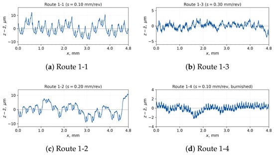
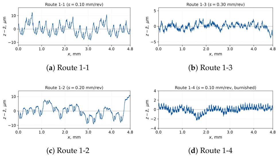
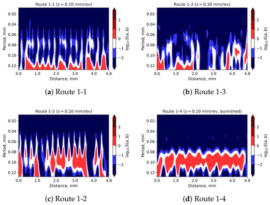
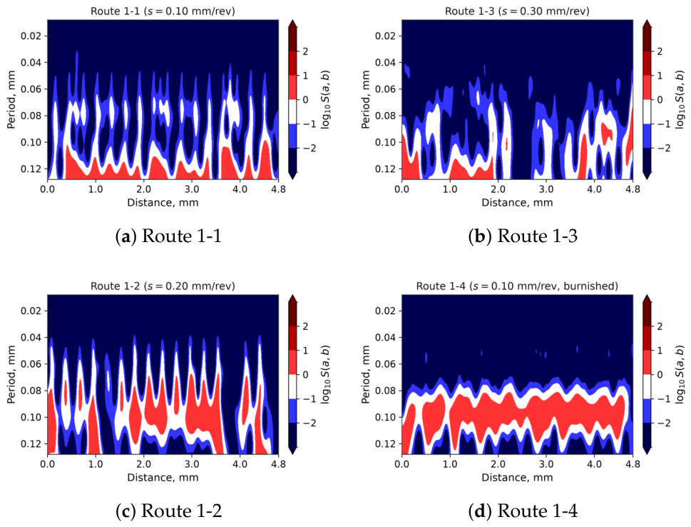
Representative Group 1 surface profiles and their corresponding scalograms are shown in Figure 3 and Figure 4, respectively.

Figure 3. Representative surface profiles for the machining routes used in Group 1 experiments.

Figure 4. Scalograms of the surface profiles for the machining routes used in Group 1 experiments.

The two processing chains examined in Group 2 were 2-1 → 2-2 → 2-3 and 2-1 → 2-4 → 2-5 → 2-6. These chains were selected to distinguish the effect of introducing finish turning before the deformation-based finishing operations.

3. Results

3.1. Baseline Comparison with Conventional Roughness Parameters (Ra and Rz)

To establish an empirical baseline and evaluate whether multiscale scalogram descriptors provide discriminative advantages over standard scalar metrics, conventional roughness parameters $R_a$ and $R_z$ were measured for all routes in Group 1 and Group 2 in accordance with ISO 4287/ISO 21920 (Table 2).

Table 2. Conventional ISO roughness parameters ($R_a$ and $R_z$) measured for Group 1 and Group 2 machining routes (mean ± standard deviation, $n=3$ profiles per route).

Group	Route	Process Sequence	${\mathit{R}}_{\mathit{a}}$ ($\mathsf{\mu }$m)	${\mathit{R}}_{\mathit{z}}$ ($\mathsf{\mu }$m)
1	1-1	Rough turning	$2.53\pm 0.05$	$12.60\pm 0.62$
	1-2	Rough turning + burnishing	$1.48\pm 0.29$	$6.46\pm 1.32$
	1-3	Rough turning + finish turning	$0.63\pm 0.08$	$3.67\pm 0.48$
	1-4	Rough turning + finish turning + burnishing	$0.32\pm 0.05$	$1.87\pm 0.29$
2 (Chain 1 & 2)	2-1	Rough turning	$3.01\pm 0.07$	$16.09\pm 0.67$
	2-2	Rough turning + ball burnishing	$0.16\pm 0.01$	$2.07\pm 0.05$
	2-3	Rough turning + ball burnishing + burnishing	$0.22\pm 0.02$	$1.92\pm 0.20$
	2-4	Rough turning + finish turning	$0.65\pm 0.16$	$3.66\pm 0.84$
	2-5	Rough turning + finish turning + ball burnishing	$0.08\pm 0.01$	$0.58\pm 0.06$
	2-6	Rough turning + finish turning + ball burnishing + burnishing	$0.22\pm 0.003$	$1.22\pm 0.02$

The empirical comparison reveals a critical metrological insight. Consider Route 2-3 (Chain 1: 2-1 → 2-2 → 2-3) and Route 2-6 (Chain 2: 2-1 → 2-4 → 2-5 → 2-6). Both routes exhibit an identical average arithmetic roughness value of $R_a=0.22\mathsf{\mu }\mathrm{m}$ ($0.22\pm 0.02\mathsf{\mu }\mathrm{m}$ for Route 2-3 vs. $0.22\pm 0.003\mathsf{\mu }\mathrm{m}$ for Route 2-6). Under conventional inspection protocols, an engineer relying strictly on $R_a$ would judge these two surfaces to be completely indistinguishable in terms of surface quality, completely overlooking their contrasting manufacturing histories. In contrast, ten-point height $R_z$ reveals a 1.6-fold difference ($1.92\mathsf{\mu }\mathrm{m}$ vs. $1.22\mathsf{\mu }\mathrm{m}$), indicating differing summit-to-valley distributions. Most decisively, the scalogram-derived heredity metric ${\eta }_{HS}^2$ for $S_{75}$ decreases from $0.1317$ in Route 2-3 to $0.0847$ in Route 2-6 (and for $I_{\max }$ drops by twenty-fold from $0.1265$ down to $0.0063$; Table 3), demonstrating a profound reduction in residual multiscale variability. This confirms empirically that scalogram descriptors provide scale-resolved sensitivity to manufacturing history that scalar roughness metrics cannot capture.

Table 3. ANOVA-based decomposition and heredity-sensitive residual variance ratio ${\eta }_{\mathrm{HS}}^2$ for selected scalogram descriptors ($I_{\max }$, $I_{\max }/I_{\mathrm{mean}}$, $S_{75}$) across Group 2 machining routes, with 95% profile-level bootstrap confidence intervals from all 27 ordered profile-level resamples.

Route	Descriptor	${\mathit{\eta }}_{\mathbf{HS}}^2$	95% Bootstrap CI	$\frac{{\mathbf{SS}}_{\mathit{I}}}{{\mathbf{SS}}_{\mathbf{tot}}}$	$\frac{{\mathbf{SS}}_{\mathit{J}}}{{\mathbf{SS}}_{\mathbf{tot}}}$	$\frac{{\mathbf{SS}}_{\mathbf{IJ}}}{{\mathbf{SS}}_{\mathbf{tot}}}$	$\frac{{\mathbf{SS}}_{\mathbf{err}}}{{\mathbf{SS}}_{\mathbf{tot}}}$
2-1	$I_{\max }$	0.3245	[0.0138; 0.4368]	0.5978	0.0777	0.0516	0.2729
	$I_{\max }/I_{\mathrm{mean}}$	0.3248	[0.0166; 0.3990]	0.6749	0.0003	0.0235	0.3013
	$S_{75}$	0.2488	[0.0630; 0.2892]	0.7301	0.0211	0.0600	0.1888
2-2	$I_{\max }$	0.8513	[0.0442; 0.9460]	0.0833	0.0654	0.0118	0.8395
	$I_{\max }/I_{\mathrm{mean}}$	0.0791	[0.0025; 0.0822]	0.9002	0.0207	0.0047	0.0744
	$S_{75}$	0.5254	[0.1081; 0.5331]	0.4324	0.0422	0.0914	0.4339
2-3	$I_{\max }$	0.1265	[0.0334; 0.1631]	0.8331	0.0403	0.0066	0.1199
	$I_{\max }/I_{\mathrm{mean}}$	0.0910	[0.0556; 0.0951]	0.9080	0.0010	0.0019	0.0891
	$S_{75}$	0.1317	[0.0724; 0.1624]	0.8035	0.0648	0.1071	0.0246
2-4	$I_{\max }$	0.1462	[0.0021; 0.1823]	0.8160	0.0378	0.0193	0.1269
	$I_{\max }/I_{\mathrm{mean}}$	0.6298	[0.1998; 0.6413]	0.3210	0.0492	0.0988	0.5310
	$S_{75}$	0.3488	[0.2056; 0.3488]	0.5653	0.0859	0.1555	0.1933
2-5	$I_{\max }$	0.2290	[0.0714; 0.2405]	0.7295	0.0416	0.0422	0.1867
	$I_{\max }/I_{\mathrm{mean}}$	0.4042	[0.1315; 0.4075]	0.5898	0.0060	0.0444	0.3598
	$S_{75}$	0.3025	[0.0288; 0.3622]	0.6173	0.0802	0.1017	0.2008
2-6	$I_{\max }$	0.0063	[0.0012; 0.0079]	0.9903	0.0034	0.0022	0.0042
	$I_{\max }/I_{\mathrm{mean}}$	0.0465	[0.0114; 0.0480]	0.9459	0.0076	0.0106	0.0359
	$S_{75}$	0.0847	[0.0006; 0.1098]	0.9031	0.0123	0.0114	0.0732

3.2. Robustness of Scalogram Descriptors Under Artificial Noise

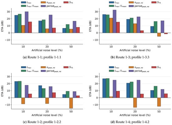
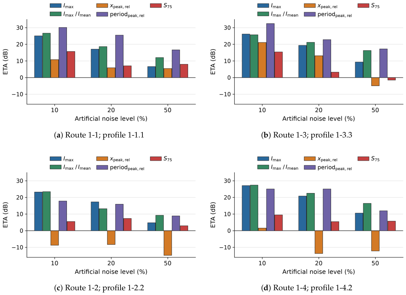
The analysis based on the Taguchi ETA metric showed that $I_{\max }$, $I_{\max }/I_{\mathrm{mean}}$, and ${\mathrm{period}}_{\mathrm{peak}}$ were the most robust descriptors in the presence of artificial noise, whereas $x_{\mathrm{peak}}$ was more sensitive to perturbation (Figure 5). This result is physically reasonable because local coordinate shifts are more strongly affected by surface nonuniformity, while energy concentration and dominant period are more stable descriptors of the machining signature [20].

Figure 5. Taguchi ETA values (signal-to-noise ratios) for representative profiles of the four Group 1 machining routes as a function of the imposed noise level (10%, 20%, and 50%). A common vertical scale is used in all panels.

3.3. Discriminative Analysis and Route Classification (Group 1)

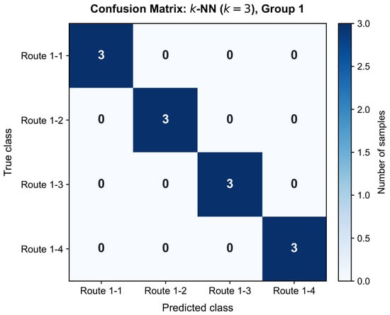
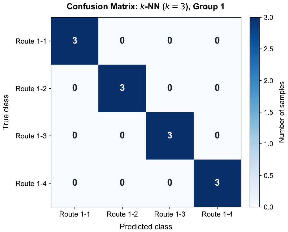
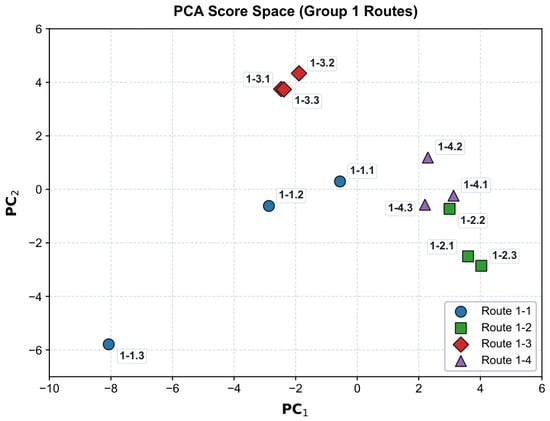
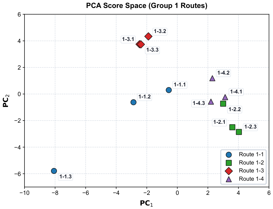
The classification analysis for Group 1 demonstrated that the proposed scalogram descriptors allow separation of the investigated machining routes under the present controlled conditions. Using leave-one-out cross-validation at the profile level, the k-NN classifier (Figure 6) assigned all held-out profiles to their correct route class, and the PCA map in the PC1–PC2 plane (Figure 7) displayed clearly separated clusters for routes 1-1 through 1-4. Given the limited number of profiles per route (three), this result should be interpreted as a proof-of-concept demonstration of route separability rather than as a generalizable estimate of classification accuracy; validation on an independent, larger dataset is required before broader claims can be made.

Figure 6. Confusion matrix for Group 1 route classification using the k-NN algorithm based on the 45-dimensional scalogram feature space.

Figure 7. Separation of Group 1 machining routes in the PCA score space (PC1–PC2) based on the extracted scalogram descriptors.

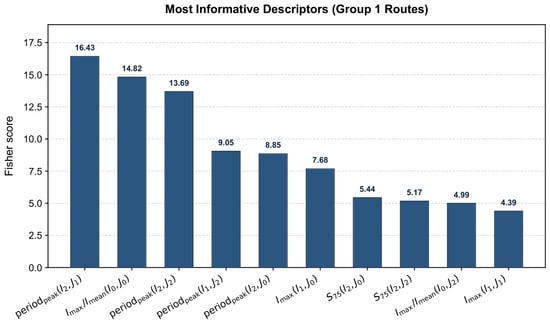
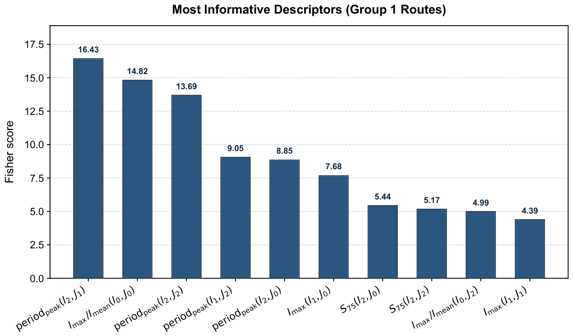
The Fisher score ranking (Figure 8) indicated that the most informative descriptors were concentrated in specific Taguchi regions and were drawn mainly from $I_{\max }$, $I_{\max }/I_{\mathrm{mean}}$, and $S_{75}$. This means that both local peak energy and the spread of the high-energy domain are essential for distinguishing the machining signature of the surface.

Figure 8. Ranking of the most informative scalogram descriptors for Group 1 routes according to the Fisher score criterion.

3.4. ANOVA Quantification of Technological Heredity (Group 2)

For Group 2 routes, values of ${\eta }_{\mathrm{HS}}^2$ varied systematically along the machining chains, although the associated bootstrap confidence intervals indicate that this variation should be interpreted with appropriate caution given the limited replication (Table 3). For the baseline route 2-1 (rough turning), ${\eta }_{\mathrm{HS}}^2$ ranged from 0.2488 ($S_{75}$) to 0.3248 ($I_{\max }/I_{\mathrm{mean}}$), with the period factor accounting for 60–73% of total variation.

The effect of ball burnishing alone (route 2-2) was descriptor-dependent: ${\eta }_{\mathrm{HS}}^2$ was low for $I_{\max }/I_{\mathrm{mean}}$ (0.0791) but elevated for $I_{\max }$ (0.8513) and $S_{75}$ (0.5254), with the elevated values dominated by the profile-to-profile residual component (${\mathrm{SS}}_{\mathrm{err}}/{\mathrm{SS}}_{\mathrm{tot}}=0.8395$ and $0.4339$, respectively) rather than by period–coordinate interaction. This indicates that ball burnishing stabilized the energy-concentration descriptor while leaving the peak-energy level and high-energy spatial occupancy more variable among the three measured profiles.

Route 2-3, in which subsequent fixed-indenter burnishing was added after ball burnishing, showed a marked reduction in ${\eta }_{\mathrm{HS}}^2$ across all three descriptors (0.1265, 0.0910, and 0.1317), with the period factor explaining 80–91% of the total variance. This is consistent with a more regular and reproducible scale-resolved surface signature after the two successive deformation-based operations.

Table 3 summarizes the updated results for $I_{\max }$, $I_{\max }/I_{\mathrm{mean}}$, and $S_{75}$, including 95% profile-level bootstrap confidence intervals from the exact distribution of all 27 ordered profile-level resamples and the separate contributions of period, coordinate, interaction, and residual variance.

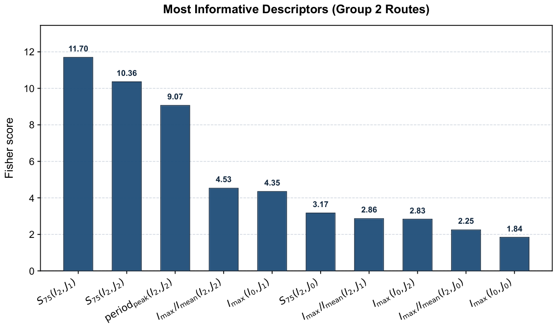
Figure 9 shows the corresponding ranking of informative descriptors used in this analysis.

Figure 9. Ranking of the most informative scalogram descriptors for Group 2 routes used for the subsequent analysis of technological heredity.

In the second chain, route 2-4 (rough + finish turning) exhibited a low ${\eta }_{\mathrm{HS}}^2$ for $I_{\max }$ (0.1462) but substantially higher values for $I_{\max }/I_{\mathrm{mean}}$ (0.6298, 95% CI [0.1998; 0.6413]) and $S_{75}$ (0.3488). The subsequent addition of ball burnishing (route 2-5) reduced these values to 0.4042 and 0.3025, respectively. The lowest ${\eta }_{\mathrm{HS}}^2$ values among all investigated routes were obtained for route 2-6 (finish turning + ball burnishing + subsequent burnishing): 0.0063 for $I_{\max }$ (95% CI [0.0012; 0.0079]), 0.0465 for $I_{\max }/I_{\mathrm{mean}}$, and 0.0847 for $S_{75}$, with 90–99% of the total variance explained by the period factor alone.

These trends indicate that, within the investigated experimental conditions, the combined application of ball burnishing and subsequent fixed-indenter burnishing produced the most regular and reproducible multiscale scalogram signature, and hence the lowest heredity-sensitive residual variability, among the studied machining routes.

3.5. Sensitivity to Scalogram Partition Resolution

The sensitivity of ${\eta }_{\mathrm{HS}}^2$ to the period–coordinate partition was evaluated by comparing the original $3\times 3$ representation with a coarser, aggregated $2\times 2$ representation (Section 2.7) (Table 4). The absolute values of ${\eta }_{\mathrm{HS}}^2$ changed for several route–descriptor combinations: for example, for route 2-1, ${\eta }_{\mathrm{HS}}^2$ for $I_{\max }$ increased from 0.3245 ($3\times 3$) to 0.4735 ($2\times 2$), whereas for route 2-4, the value for $S_{75}$ decreased from 0.3488 to 0.1770. This confirms that the numerical value of ${\eta }_{\mathrm{HS}}^2$ depends on the spatial and period resolution of the analysis.

Table 4. Comparison of unexplained variance ratios ${\eta }_{\mathrm{HS}}^2$ across $3\times 3$ and $2\times 2$ partition schemes for Group 2 routes. All three descriptors ($I_{\max }$, $I_{\max }/I_{\mathrm{mean}}$, and $S_{75}$) are reported.

Route	${\mathit{I}}_{\max }$		${\mathit{I}}_{\max }/{\mathit{I}}_{\mathbf{mean}}$		${\mathit{S}}_{75}$
	$\mathbf{3}\times \mathbf{3}$	$\mathbf{2}\times \mathbf{2}$	$\mathbf{3}\times \mathbf{3}$	$\mathbf{2}\times \mathbf{2}$	$\mathbf{3}\times \mathbf{3}$	$\mathbf{2}\times \mathbf{2}$
2-1	0.3245	0.4735	0.3248	0.2688	0.2488	0.2436
2-2	0.8513	0.8174	0.0791	0.0888	0.5254	0.6731
2-3	0.1265	0.1331	0.0910	0.0534	0.1317	0.1295
2-4	0.1462	0.0723	0.6298	0.4334	0.3488	0.1770
2-5	0.2290	0.1909	0.4042	0.2765	0.3025	0.2224
2-6	0.0063	0.0036	0.0465	0.0216	0.0847	0.0764

Despite this partition dependence, the principal route-dependent conclusion was preserved. Route 2-6 exhibited the lowest ${\eta }_{\mathrm{HS}}^2$ among all routes for all three descriptors under both partition schemes (0.0063 vs. 0.0036 for $I_{\max }$; 0.0465 vs. 0.0216 for $I_{\max }/I_{\mathrm{mean}}$; 0.0847 vs. 0.0764 for $S_{75}$), and route 2-3 retained comparatively low values for $I_{\max }$ and $S_{75}$ (0.1265 vs. 0.1331; 0.1317 vs. 0.1295). These results indicate that the observed regularization associated with the final deformation-based finishing operations is not an artifact of the specific $3\times 3$ grid, whereas the absolute magnitude of ${\eta }_{\mathrm{HS}}^2$ should be interpreted relative to the chosen partition resolution. The point estimates for both grids were calculated from the same archived profile-level feature matrix. The $2\times 2$ values were obtained by the deterministic aggregation defined in Section 2.7; no random sampling enters these point estimates. (The complete factor-by-factor ANOVA decomposition across all six routes is reported in Supplementary Materials, Table S1).

3.6. PCA Interpretation of Machining-Route Trajectories

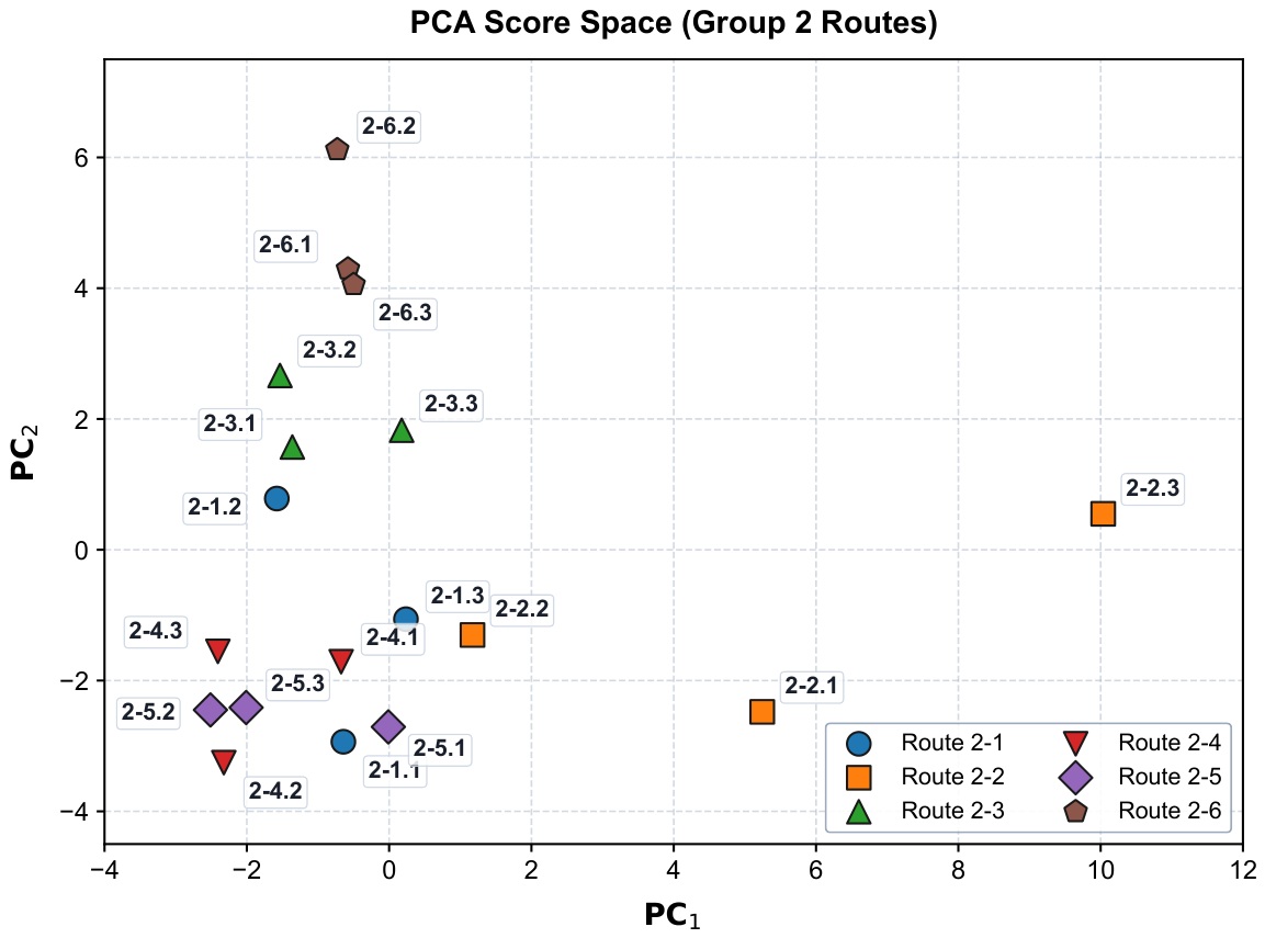
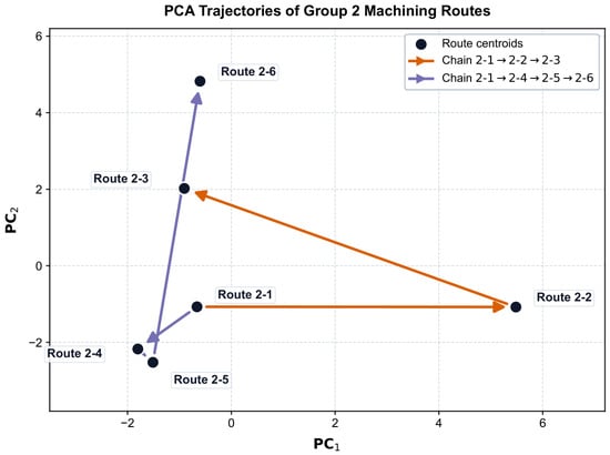
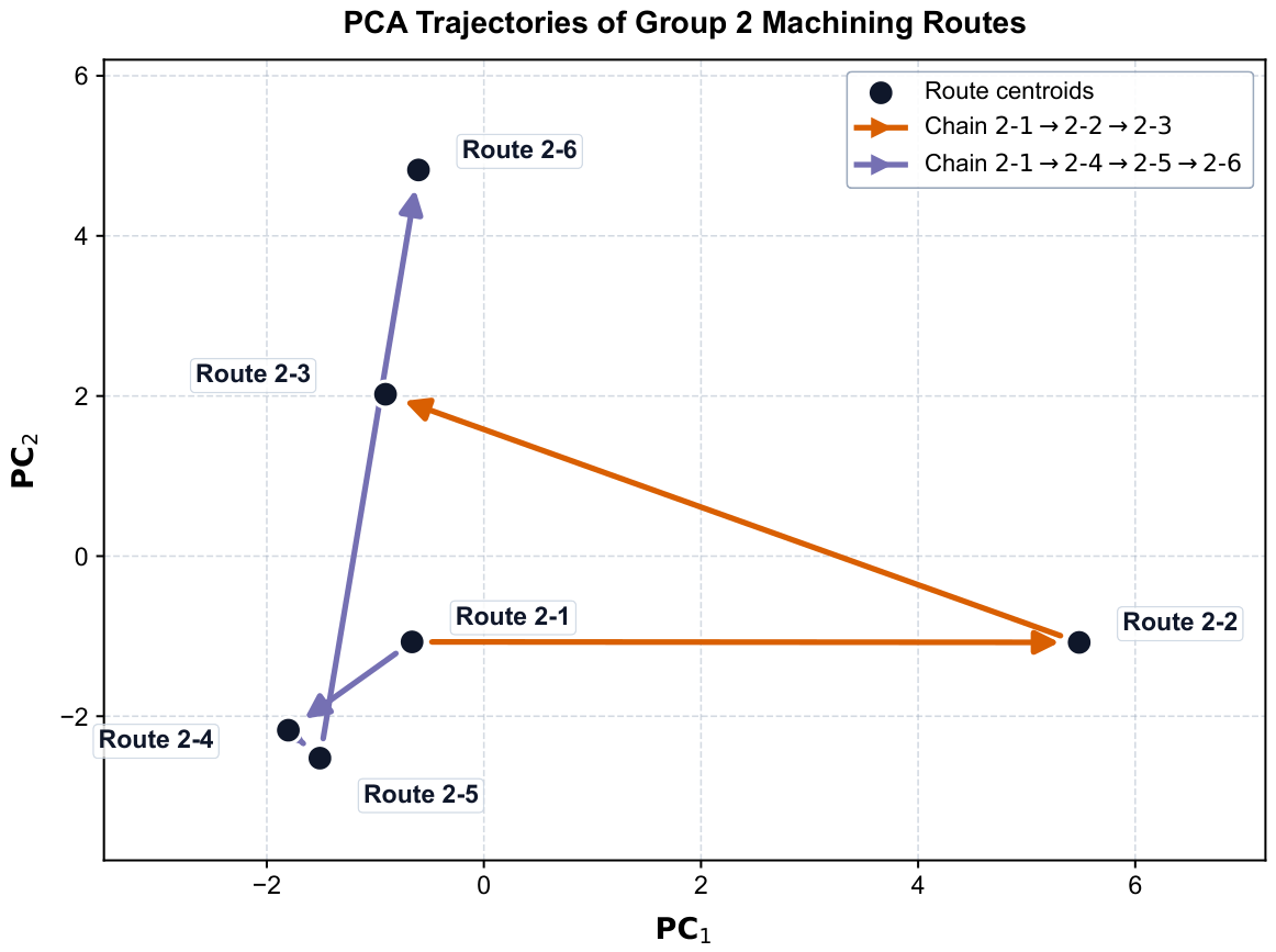
The PCA results for Group 2 (Figure 10 and Figure 11) provide a geometric interpretation of technological heredity. The routes form two distinct trajectories in PC space: 2-1 → 2-2 → 2-3 and 2-1 → 2-4 → 2-5 → 2-6. The first trajectory reflects the effect of adding ball burnishing and then burnishing directly after rough turning, while the second reflects the insertion of finish turning before the deformation-based finishing stages.

Figure 10. PCA clusters of Group 2 machining routes in the PC1–PC2 plane.

Figure 11. PCA trajectories of Group 2 machining routes in the PC1–PC2 plane, showing the evolution of surface signatures along the chains 2-1 → 2-2 → 2-3 and 2-1 → 2-4 → 2-5 → 2-6.

Routes with high unexplained variance formed less compact clusters and occupied more widely separated positions in PCA space, whereas routes with burnishing exhibited tighter clustering and more stable positions. This interpretation supports the combined use of PCA and ANOVA: PCA reveals the geometry of route evolution, while ANOVA quantifies how much of the surface signature remains dominated by technological heredity.

4. Discussion

The results show that a scalogram derived from the Morlet wavelet transform retains scale-localized information about the distribution of profile energy that a single scalar roughness parameter cannot express. This is not presented as evidence that scalogram descriptors are superior to, or should replace, conventional parameters such as $R_a$, $R_q$, or $R_z$; rather, it demonstrates that they provide complementary information on where and how strongly specific periodic components occur along the profile. Conventional roughness parameters remain the standard, well-validated basis for surface-quality specification, and the present framework is intended to supplement, not substitute, this basis in applications where information about spatial localization and multiscale structure is additionally required [6,8,21,22,23]. The two routes had the same $R_a=0.22\mathsf{\mu }\mathrm{m}$ but different $R_z$ values (1.92 and 1.22 $\mathsf{\mu }\mathrm{m}$). Their ${\eta }_{\mathrm{HS}}^2$ values also differed: 0.1265 and 0.0063 for $I_{\max }$, and 0.1317 and 0.0847 for $S_{75}$. Thus, $R_a$ alone did not distinguish this pair, whereas $R_z$ and the scalogram-derived ratios described different amplitude- and scale-resolved aspects of the profiles.

For Group 2, profile-level leave-one-out validation with a 1-nearest-neighbor classifier gave 7/18 correct classifications (38.9%) from the 45 scalogram descriptors and 18/18 (100%) from $R_a$, $R_q$, and $R_z$ (Supplementary Materials, Figure S1). Thus, for these six routes, the three scalar amplitude parameters separated the route classes more effectively than the high-dimensional scalogram vector. The Group 2 scalogram analysis is therefore used here for descriptive ANOVA-based decomposition of scale- and position-dependent variability, not as evidence of superior route classification. The equal $R_a$ value of 0.22 $\mathsf{\mu }\mathrm{m}$ for Routes 2-3 and 2-6 nevertheless shows that one scalar parameter does not encode all route-dependent differences; $R_z$ and the scalogram-derived ratios provide complementary information. Classification performance and generalizability require evaluation with larger independent datasets.

The Taguchi L9 partition is not only a convenient way to divide the scalogram but also a physically meaningful framework for separating wavelength-related effects from effects associated with spatial position [25].

This interpretation should be applied with care. A high value of ${\eta }_{\mathrm{HS}}^2$ indicates that the descriptor cannot be adequately described by the additive main effects of period and coordinate alone; however, this residual variability combines two distinct sources: non-additive period–coordinate coupling (${\mathrm{SS}}_{IJ}$) and profile-to-profile variation within the same route (${\mathrm{SS}}_{\mathrm{err}}$). In the present dataset, the latter component dominates ${\eta }_{\mathrm{HS}}^2$ for several route–descriptor combinations (e.g., route 2-2, $I_{\max }$), indicating limited repeatability of certain descriptors rather than a purely structural heredity effect. We therefore use ${\eta }_{\mathrm{HS}}^2$ as a heredity-sensitive indicator rather than as a direct, absolute coefficient of technological heredity: routes with a low, consistently reproducible ${\eta }_{\mathrm{HS}}^2$ across replicated profiles (such as route 2-6) are interpreted as producing a more regular and less heredity-affected surface signature, whereas routes with high but poorly reproducible ${\eta }_{\mathrm{HS}}^2$ (wide bootstrap confidence intervals) require additional replicated measurements before firm heredity-related conclusions can be drawn [1,2,28].

The physical mechanism governing this heredity attenuation is directly rooted in the mechanics of surface plastic deformation (SPD) during burnishing. During initial rough and finish turning, the cutting insert generates pronounced, periodic cusps and micro-grooves governed by tool feed and nose radius, accompanied by substantial subsurface work hardening [4]. When subsequent ball burnishing is applied, the high contact pressure exceeding the material yield point causes localized plastic flow of the asperity summits, displacing metal into the adjacent micro-valleys [13,16]. In the first processing chain (2-1 → 2-2 → 2-3), ball burnishing applied directly over coarse rough-turned ridges ($R_a=3.01\mathsf{\mu }\mathrm{m}$) flattens the peaks but leaves deep residual valleys, explaining the relatively high unexplained variance in $S_{75}$ (${\eta }_{HS}^2=0.5254$). Subsequent sliding diamond burnishing with a fine spherical diamond tip ($r=3.0$ mm) under normal force further smooths these secondary micro-irregularities, driving ${\eta }_{HS}^2$ down to $0.1317$.

In the second processing chain (2-1 → 2-4 → 2-5 → 2-6), the insertion of finish turning removes the coarse primary peaks but introduces fine, high-frequency feed marks that interact with underlying work-hardened layers, resulting in elevated structural complexity (${\eta }_{HS}^2=0.3488$ for $S_{75}$ in route 2-4 and $0.3025$ in route 2-5). Subsequent sequential ball burnishing and diamond burnishing systematically obliterate these harmonic feed marks. The final diamond burnishing pass establishes a highly uniform, regularized micro-texture governed entirely by the elastoplastic contact zone of the diamond indenter, yielding the minimum residual heredity variance observed (${\eta }_{HS}^2=0.0847$ for $S_{75}$ and $0.0063$ for $I_{\max }$). These observations are in strong agreement with recent findings by Maximov et al. [14,15] and Kułakowska and Bohdal [12], who demonstrated that combined plastic deformation finishing completely suppresses prior cutting texture in austenitic steels.

From an engineering perspective, the proposed method can support route identification, optimization of finishing sequences, and design of more robust surface-generation processes, used alongside—not instead of—conventional roughness-based quality control. A practical implementation would involve constructing a reference library of validated scalogram signatures for a given material–machine–tool system; a newly measured profile could then be processed with the same CWT, partition, and feature-extraction procedure and compared against this library. The present study demonstrates the feasibility of this descriptor representation under controlled laboratory conditions, using a single material, shaft diameter, and lathe tooling setup; it does not yet establish reliable identification of an unknown or previously unseen process history under general industrial conditions. Extension to other materials, hardness ranges, tool geometries, and milled or ground surfaces, together with independent validation using a larger number of replicated profiles, is required before the framework can be considered for near-line or in-line monitoring applications [4,12].

From a computational and industrial perspective, the proposed CWT–Taguchi pipeline is fully deterministic and algorithmically lightweight. On a standard modern workstation, continuous wavelet transformation and 45-dimensional feature extraction require less than $0.5$ s per $4.8$ mm profile trace. This computational efficiency demonstrates the feasibility of incorporating scalogram descriptors into near-line metrological inspection or digital-twin manufacturing systems for automated quality monitoring.

Several limitations of the present study must be acknowledged:

1.

The experimental campaign investigated a single workpiece material (12Kh18N10T/ AISI 321 austenitic stainless steel), a single cylindrical diameter (40 mm), and a single center lathe tooling setup. Extending the framework to high-strength steels, titanium alloys, or non-ferrous materials with differing strain-hardening characteristics will require calibrating material-specific scalogram feature boundaries.

2.

The sample size of three profiles per route ($n=3$) represents a laboratory proof-of-concept design. The leave-one-out validation was conducted at the profile level, and the exact bootstrap distribution was obtained by enumerating all 27 ordered profile-level resamples; its percentile intervals are descriptive because only three profiles were available. Full industrial implementation requires larger training datasets to account for tool wear, machine thermal drift, and batch-to-batch material variations.

3.

The principal route ordering was preserved under the aggregated $2\times 2$ representation, but the absolute ${\eta }_{\mathrm{HS}}^2$ values remained partition-dependent. Adaptive or continuous frequency-band segmentation should be evaluated in future work.

5. Conclusions

The results support profile-based route discrimination for Group 1 and descriptive assessment of scale- and position-dependent residual variability for Group 2:

1.

The five descriptors extracted in each of the nine Taguchi cells formed a 45-dimensional representation of the scale- and position-dependent profile structure. Its discrimination performance depended on the route group and validation setting. Among the descriptors, $I_{\max }$, $I_{\max }/I_{\mathrm{mean}}$, and ${\mathrm{period}}_{\mathrm{peak}}$ showed the highest robustness under artificial noise, while $I_{\max }$, $I_{\max }/I_{\mathrm{mean}}$, and $S_{75}$ were used in the heredity analysis.

2.

The baseline comparison showed complementarity rather than universal superiority. Routes 2-3 and 2-6 had identical $R_a=0.22\mathsf{\mu }\mathrm{m}$ but different $R_z$ values (1.92 and 1.22 $\mathsf{\mu }\mathrm{m}$). Their ${\eta }_{\mathrm{HS}}^2$ values decreased from 0.1265 to 0.0063 for $I_{\max }$ and from 0.1317 to 0.0847 for $S_{75}$. For the complete Group 2 classification task, however, $R_a$, $R_q$, and $R_z$ outperformed the 45-dimensional scalogram representation under profile-level 1-nearest-neighbor validation (18/18 versus 7/18 correct classifications).

3.

For the first group of machining routes, PCA, Fisher scores, and leave-one-out k-NN classification demonstrated separability of the four investigated routes under the present controlled conditions. Given the limited number of profiles per route, this result is presented as a proof-of-concept demonstration; broader generalization requires validation on an independent, larger dataset.

4.

For the second group, a profile-replicated two-way ANOVA and the heredity-sensitive residual variance ratio ${\eta }_{\mathrm{HS}}^2=({\mathrm{SS}}_{IJ}+{\mathrm{SS}}_{\mathrm{err}})/{\mathrm{SS}}_{\mathrm{tot}}$, reported with 95% profile-level bootstrap confidence intervals, provided a physically interpretable, though not absolute, indicator of technological heredity. The lowest and most reproducible values were observed for the route combining ball burnishing and subsequent burnishing (${\eta }_{\mathrm{HS}}^2=0.0063$–$0.0847$ depending on the descriptor), while several intermediate routes (e.g., route 2-2 for $I_{\max }$; route 2-4 for $I_{\max }/I_{\mathrm{mean}}$) showed elevated and less reproducible values, reflecting the combined influence of period–coordinate interaction and profile-to-profile variability. A partition-sensitivity check ($3\times 3$ vs. $2\times 2$) retained the same principal route ordering, although the absolute ratios changed with the period–coordinate resolution.

5.

The present findings are limited to 12Kh18N10T (AISI 321-equivalent) stainless-steel shafts of 40 mm diameter, processed with the specified turning and burnishing tools, and are based on three replicated longitudinal profiles per route. Route separability was demonstrated only for Group 1 under the reported experimental and classification settings; Group 2 was analyzed primarily through variance decomposition. Industrial implementation and generalization require independent validation on larger datasets spanning varied materials, workpiece geometries, and cutting regimes.

6.

Within the investigated dataset, the combined scalogram–Taguchi–PCA–ANOVA framework provides scale- and position-resolved descriptors for Group 1 route discrimination and descriptive comparison of residual multiscale variability across Group 2 processing chains.

References

- Zmarzły, P. Analysis of Technological Heredity in the Production of Rolling Bearing Rings Made of AISI 52100 Steel Based on Waviness Measurements. Materials 2022, 15, 3959. [Google Scholar] [CrossRef] [Scilit] [PubMed]
- Kuritsyn, D.N.; Siluyanova, M.V.; Kuritsyna, V.V. A Model of Technological Inheritance for Methods of Technological Decision-Making in Manufacturing Operations in the Engine Industry. Russ. Eng. Res. 2024, 44, 1032–1035. [Google Scholar] [CrossRef] [Scilit]
- Li, L.; Zhang, W.; Wang, J.; Ruan, X.; Li, L.; Xie, M. Multiscale characterization and contact performance analysis of machining surfaces. Sci. Rep. 2023, 13, 9710. [Google Scholar] [CrossRef] [Scilit] [PubMed]
- Maximov, J.; Duncheva, G.; Anastasov, K.; Ichkova, M.; Daskalova, P. Influence of Previous Turning on the Surface Integrity Stability of Diamond-Burnished Medium-Carbon Steel. Machines 2025, 13, 864. [Google Scholar] [CrossRef] [Scilit]
- Thamizhmanii, S.; Saparudin, S.; Hasan, S. Analyses of surface roughness by turning process using Taguchi method. J. Achiev. Mater. Manuf. Eng. 2007, 20, 503–506. [Google Scholar]
- Grochała, D.; Grzejda, R.; Parus, A.; Berczyński, S. The Wavelet Transform for Feature Extraction and Surface Roughness Evaluation after Micromachining. Coatings 2024, 14, 210. [Google Scholar] [CrossRef] [Scilit]
- Yesilli, M.C.; Chen, J.; Khasawneh, F.A.; Guo, Y. Automated surface texture analysis via Discrete Cosine Transform and Discrete Wavelet Transform. Precis. Eng. 2022, 77, 141–152. [Google Scholar] [CrossRef] [Scilit]
- Wu, Y.; Liu, L.; Huang, L.; Wang, Z. A monitoring method for surface roughness of γ-TiAl alloy based on deep learning of time–frequency diagram. Int. J. Adv. Manuf. Technol. 2023, 129, 2989–3007. [Google Scholar] [CrossRef] [Scilit]
- Shumetova, A.A.; Mel’nikov, P.A. Identification of the Microrelief after Abrasive Machining by Wavelet Analysis. Russ. Eng. Res. 2024, 44, 1819–1822. [Google Scholar] [CrossRef] [Scilit]
- Bobrovskij, I.; Khaimovich, A.; Bobrovskij, N.; D’yakonov, A. Determination of Wide Burnishing Energy-Force Parameters Based on Constructing the Kinematically Admissible Velocity Field. Metals 2020, 10, 46. [Google Scholar] [CrossRef] [Scilit]
- Bobrovskij, I.; Bobrovskij, N.; Khaimovich, A.; Travieso-Rodriguez, J.A. Impacts of Surface Texture and Nature of Friction on Energy-Force Efficiency of Surface Plastic Deformation during Burnishing. Metals 2022, 12, 1568. [Google Scholar] [CrossRef] [Scilit]
- Kułakowska, A.; Bohdal, Ł. Surface Characterization of Carbon Steel after Rolling Burnishing Treatment. Metals 2024, 14, 31. [Google Scholar] [CrossRef] [Scilit]
- Swirad, S. Changes in Areal Surface Textures Due to Ball Burnishing. Materials 2023, 16, 5904. [Google Scholar] [CrossRef] [Scilit] [PubMed]
- Maximov, J.; Duncheva, G.; Ichkova, M.; Anastasov, K. Optimal Diamond Burnishing of Chromium–Nickel Austenitic Stainless Steels Based on the Finishing Process–Surface Integrity–Operating Behavior Correlations. Metals 2025, 15, 574. [Google Scholar] [CrossRef] [Scilit]
- Maximov, J.; Duncheva, G.; Anchev, A.; Dunchev, V.; Anastasov, K.; Argirov, Y. Sustainable Diamond Burnishing of Chromium–Nickel Austenitic Stainless Steels: Effects on Surface Integrity and Fatigue Limit. Appl. Sci. 2024, 14, 9031. [Google Scholar] [CrossRef] [Scilit]
- Chodór, J.; Kukiełka, L.; Chomka, G.; Bohdal, Ł.; Patyk, R.; Kowalik, M.; Trzepieciński, T.; Radchenko, A.M. Using the FEM Method in the Prediction of Stress and Deformation in the Processing Zone of an Elastic/Visco-Plastic Material during Diamond Sliding Burnishing. Appl. Sci. 2023, 13, 1963. [Google Scholar] [CrossRef] [Scilit]
- Josso, B.; Burton, D.R.; Lalor, M.J.; Watson, S. Frequency normalised wavelet transform for surface roughness analysis and characterisation. Wear 2002, 252, 491–500. [Google Scholar] [CrossRef] [Scilit]
- Mallat, S. A Wavelet Tour of Signal Processing, 2nd ed.; Academic Press: San Diego, CA, USA, 1999. [Google Scholar]
- Daubechies, I. Ten Lectures on Wavelets; SIAM: Philadelphia, PA, USA, 1992. [Google Scholar]
- Wu, Y.-H.; Ren, H.-Y. Analysis of realistic rough surface for its globally dominant parameters using continuous wavelets. Appl. Math. Mech. 2014, 35, 741–748. [Google Scholar] [CrossRef] [Scilit]
- Karolczak, P.; Kowalski, M. Assessment of the Possibility of Using the Continuous Wavelet Transform and Fourier Transform to Analyse Geometric Structures Obtained on the Surface of Turned High-Molecular Polymers. Manuf. Technol. 2025, 25, 24–36. [Google Scholar] [CrossRef] [Scilit]
- Ghosh, S.; Knoblauch, R.; El Mansori, M.; Corleto, C. Accelerated 2D continuous wavelet transform for scale-resolved surface evolution across tool wear states in stainless steel milling. Int. J. Adv. Manuf. Technol. 2026, 143, 6317–6336. [Google Scholar] [CrossRef] [Scilit]
- Chen, G.; Peng, W.; Tu, J.; Wang, W.; Zhao, H. Classification of drilling surface roughness on computer numerical control (CNC) machine tools based on Mobilenet_v3_small_improved. Mech. Sci. 2024, 15, 567–586. [Google Scholar] [CrossRef] [Scilit]
- Lee, G.; Gommers, R.; Waselewski, F.; Wohlfahrt, K.; O’Leary, A. PyWavelets: A Python package for wavelet analysis. J. Open Source Softw. 2019, 4, 1237. [Google Scholar] [CrossRef] [Scilit]
- Raman, R.S.; Kukreja, N.; Singh, N. Process parameters optimization through Taguchi and ANOVA analysis: A review. Int. J. Curr. Eng. Technol. 2014, 4, 1514–1518. [Google Scholar] [CrossRef] [Scilit]
- Patel, N.S.; Parihar, P.L.; Makwana, J.S. Parametric optimization to improve the machining process by using Taguchi method: A review. Mater. Today Proc. 2021, 44, 3059–3068. [Google Scholar] [CrossRef] [Scilit]
- Taguchi, G.; Chowdhury, S.; Wu, Y. Taguchi’s Quality Engineering Handbook; John Wiley & Sons: Hoboken, NJ, USA, 2005. [Google Scholar]
- Montgomery, D.C. Design and Analysis of Experiments, 5th ed.; John Wiley & Sons: New York, NY, USA, 2001. [Google Scholar]
- ISO 3274:1996; Geometrical Product Specifications (GPS)—Surface Texture: Profile Method—Nominal Characteristics of Contact (Stylus) Instruments. International Organization for Standardization: Geneva, Switzerland, 1996.
- ISO 4287:1997; Geometrical Product Specifications (GPS)—Surface Texture: Profile Method—Terms, Definitions and Surface Texture Parameters. International Organization for Standardization: Geneva, Switzerland, 1997.
- ISO 21920-2:2021; Geometrical Product Specifications (GPS)—Surface Texture: Profile—Part 2: Terms, Definitions and Surface Texture Parameters. International Organization for Standardization: Geneva, Switzerland, 2021.
- ISO 16610-21:2011; Geometrical Product Specifications (GPS)—Filtration—Part 21: Linear Profile Filters: Gaussian Filters. International Organization for Standardization: Geneva, Switzerland, 2011.
Disclaimer/Publisher’s Note: The statements, opinions and data contained in all publications are solely those of the individual author(s) and contributor(s) and not of MDPI and/or the editor(s). MDPI and/or the editor(s) disclaim responsibility for any injury to people or property resulting from any ideas, methods, instructions or products referred to in the content. |
© 2026 by the authors. Licensee MDPI, Basel, Switzerland. This article is an open access article distributed under the terms and conditions of the Creative Commons Attribution (CC BY) license.