


Simple Summary
Blow flies are important in death investigations because the age and identity of insects collected from human remains can help investigators estimate when insect colonization occurred. However, this evidence must be interpreted using information about which species are active in a particular place and season. Arizona contains markedly different desert and mountain environments, but information about its blow fly communities remains limited. To our knowledge, this is the first standardized multiyear survey to compare blow fly communities among three fixed locations representing central, southern, and northern Arizona respectively. We surveyed blow flies monthly from May 2020 through December 2024 and collected 7972 flies representing 11 species. The locations differed in species diversity, seasonal activity, and dominant species. Glendale had many flies during spring but no captures during July, August, or September, when temperatures were highest. Flagstaff supported the greatest species diversity and a longer period of summer activity, while Tucson had fewer flies but a comparatively diverse community. These findings show that blow fly information from one Arizona location may not accurately represent another. These findings provide baseline information about which species were active at three fixed Arizona sites and when they were recovered. They show why observations from one location or season should not automatically be applied elsewhere. The absence of captures during extreme heat suggests reduced adult activity or attraction to bait but does not demonstrate that colonization was delayed or ceased.
Abstract
Regional information on blow fly occurrence and seasonal activity is necessary for interpreting entomological evidence, but contemporary data remain limited for Arizona. This study compared adult blow fly communities at one fixed sampling site in each of three Arizona locations: Glendale, Tucson, and Flagstaff. Adult blow flies were sampled monthly from May 2020 through December 2024 using 24-h baited traps. Temperature and relative humidity were recorded using on-site data loggers. A total of 7972 blow flies representing 11 species were collected across 168 sampling events. Mean monthly abundance did not differ significantly among sites, although species richness, Shannon diversity, Simpson diversity, and zero-capture frequency differed. The Glendale site had the lowest diversity and greatest frequency of zero captures, whereas the Flagstaff site had the greatest richness and diversity. Lucilia sericata was the most abundant species overall, followed by Calliphora latifrons, Phormia regina, and Lucilia mexicana. Species composition and seasonal activity also varied among sites. The Glendale site exhibited a concentrated spring peak and no captures during July–September, whereas the Flagstaff site supported a broader warm-season activity period. The absence of captures in Glendale during the hottest summer months suggests that extreme heat may suppress adult blow fly activity, affecting the interpretation of insect evidence used for postmortem interval estimation in hot, arid environments. These findings provide a contemporary multiyear baseline for three fixed Arizona sites and show that species absence and seasonal expectations from one location should be applied cautiously elsewhere or when inferring a maximum postmortem interval.
1. Introduction
Blow flies (Diptera: Calliphoridae) are among the most important arthropods encountered during medicolegal death investigations. Many calliphorid species locate decomposing remains rapidly and use carrion as a nutritional resource for the adults and their offspring. As their immature development is strongly influenced by temperature, the age of blow fly eggs, larvae, or pupae recovered from remains can be used to generate a development-based estimate of the minimum postmortem interval (minPMI). The species present may also assist with reconstructing circumstances surrounding death, including whether remains were moved between environments or were inaccessible to insects during part of the postmortem period [1,2,3]. The forensic interpretation of insect evidence therefore depends on species-specific developmental data and an understanding of when and where individual species are likely to occur.
The abundance, activity, and composition of blow fly communities are influenced by interacting biotic and abiotic factors. Temperature affects adult flight, resource detection, oviposition, survival, and immature development, while humidity and precipitation may influence adult activity and the persistence of carrion resources. Blow fly assemblages may also vary with elevation, habitat, urbanization, season, geographic region and level of corpse exposure. Studies conducted in different parts of the world have demonstrated substantial seasonal and habitat-associated changes in calliphorid abundance and community composition [4,5]. Temperature-dependent differences in oviposition behavior have also been reported for forensically important species, including Lucilia sericata (Meigen, 1826) and Phormia regina (Meigen, 1826), indicating that environmental conditions may affect not only development following colonization but also the probability and timing of colonization itself [6]. Variation in colonization timing is relevant to succession-based interpretation but does not alter a development-based minPMI estimate.
Regional surveys establish which forensically important species are present and seasonally active, helping practitioners evaluate whether taxa recovered from remains are consistent with local expectations and identifying species for which suitable developmental data are lacking. Seasonal occurrence may also provide context for insects or empty puparia recovered from older remains. Conversely, periods when normally common species are inactive can demonstrate why their absence should not, by itself, be used to infer a maximum postmortem interval. These applications require geographically and seasonally appropriate baseline data. Such information is particularly important in Arizona, where low-elevation deserts experience prolonged extreme heat and aridity, while high-elevation northern environments have cooler summers and freezing winters.
Published information on Arizona blow fly populations remains limited and geographically fragmented. Deonier [7] established an important historical baseline for species distribution and seasonal abundance in southern Arizona, although these older data may not represent contemporary communities. Baumgartner [8] subsequently confirmed the introduced Chrysomya rufifacies (Macquart, 1843) in Arizona, illustrating that the state’s calliphorid fauna and species distributions are not static. In a year-long Phoenix survey, Meeds et al. [9] collected nine species, primarily L. sericata, Calliphora latifrons Hough, 1899, and Lucilia mexicana Macquart, 1843. Abundance varied seasonally with temperature and relative humidity, and no flies were captured during the hottest sampling periods. This finding suggests that extreme desert heat may suppress adult activity and demonstrates why the absence of a normally expected species should not, by itself, be used to infer a maximum postmortem interval. Kahler and Weidner [10] documented seasonal and elevational differences among blow fly communities in northwestern Arizona. Twelve species were recorded, with C. latifrons and Ph. regina among the most abundant. Their study also reported the northernmost Arizona record of Ch. rufifacies and the first state records of Cynomya cadaverina Robineau-Desvoidy, 1830 and Calliphora alaskensis (Shannon, 1923). Together, these studies demonstrate the ecological diversity of Arizona’s blow fly fauna and the need for contemporary sampling across distinct regions.
Despite previous Arizona surveys, contemporary comparisons among central, southern, and northern regions remain limited. Historical research focused primarily on southern Arizona, whereas recent studies examined Phoenix and northwestern Arizona. To our knowledge, no standardized multiyear study has directly compared blow fly communities at fixed sites in Glendale, Tucson, and Flagstaff using a consistent sampling design. These sites represent low-desert, intermediate-elevation desert, and high-elevation montane environments spanning approximately 1750 m in elevation. Comparing them can document geographic and seasonal differences in adult communities and indicate when observations from one Arizona location should be applied cautiously elsewhere. Repeated carrion-baited trapping permits standardized comparisons of adult abundance and composition, and previous research has shown that such traps provide useful information on Diptera likely to arrive early at carrion [11]. However, trap captures measure adult presence and activity rather than colonization of human remains or large animal carcasses.
This study aimed to characterize and compare adult blow fly communities at one fixed sampling site in each of three Arizona locations: Glendale, Tucson, and Flagstaff. Monthly trapping from May 2020 through December 2024 was used to evaluate variation in abundance, richness, diversity, and community composition among sites, months, and years, as well as associations with trap-day maximum temperature, minimum temperature, and relative humidity. Because elevation was confounded with location, it was not treated as an independent effect. The study was intended to establish contemporary baseline data for the three sampled sites and improve understanding of the geographic and seasonal availability of forensically important blow flies in Arizona.
2. Materials and Methods
2.1. Study Locations
Adult blow fly populations were surveyed at three locations in Arizona, USA: Glendale, Tucson, and Flagstaff. The locations represented contrasting climatic, elevational, and habitat conditions. The Glendale site (33.60731° N, 112.15859° W) was located within an open, unshaded urban area in the central Sonoran Desert at an approximate elevation of 350 m. The Tucson site (32.22798° N, 111.03888° W) was located within an open natural area in southern Arizona at approximately 728 m. The Flagstaff site (35.22669° N, 111.55697° W) was situated within a wooded natural area with limited shade at approximately 2106 m. Approximately 1750 m of elevation separated the lowest and highest sampling locations. A single fixed sampling site was used within each location throughout the study to maintain consistency among sampling dates. The study was designed as a standardized longitudinal comparison of three fixed sites rather than as a spatially replicated assessment of each metropolitan region. Repeated monthly sampling provided temporal replication at each site, but multiple sites were not sampled within Flagstaff, Glendale, or Tucson. Consequently, comparisons were interpreted as differences among the three sampled sites rather than estimates applicable to the entirety of each metropolitan region. Location was treated as a categorical site-level variable in subsequent analyses. Elevation was not treated as an independently replicated predictor because each sampling site was associated with a single elevation.
2.2. Sampling Design and Specimen Collection
Sampling was conducted monthly by trained graduate students from 1 May 2020 through 20 December 2024, following the same collection protocol. Approximately 27–30 days were provided between each sampling period. Sampling occurred concurrently at the three locations on each collection date. One 24-h sampling event was conducted at each location per month. This design provided 56 repeated temporal observations at each fixed site but no within-location spatial replication. Sampling during 2020 covered May through December, whereas complete monthly sampling was conducted from January through December during 2021–2024. A commercial outdoor fly trap (RESCUE! model FTR-SF4; Sterling International, Inc., Spokane, WA, USA) was deployed at each site. Each trap was baited with approximately 200 g of chicken liver purchased fresh, frozen immediately, and thawed for 24 h at approximately 20 °C before field deployment. The liver was placed in the middle of the trap. Flies entered through the top funnel entrance and were retained within the chamber, which was sealed using the trap’s built-in closure mechanism before specimens were removed. Traps were deployed at or as close as practicable to ground level, and their positions remained consistent throughout the study.
Trap placement remained consistent within each location throughout the study. At the end of each 24-h deployment, a hand-held insect net was used to collect adult blow flies observed flying immediately around or landing on the baited trap. Netting was not conducted away from the trap or elsewhere within the surrounding habitat. Trap- and net-collected specimens were combined during processing, and capture method was not recorded separately for individual specimens. At the end of each 24-h sampling period, collected flies were transferred to a killing jar containing acetone (Fisher Scientific, Waltham, MA, USA) and then preserved in 80% ethanol. Specimens were then transported to Arizona State University for preservation, identification, and enumeration.
2.3. Specimen Preservation and Identification
Following transport to Arizona State University, specimens were stored at −20 °C until identification. The preservation method used for each collection was recorded. Before identification, ethanol-preserved specimens were removed from the preservative and examined using a stereomicroscope. Adult calliphorids were identified morphologically to species using the taxonomic keys and diagnostic descriptions provided by Marshall et al. [12] and Byrd and Tomberlin [13]. Species identification was performed by graduate researchers, each with more than two years of experience identifying calliphorid flies using established taxonomic keys. Uncertain identifications were reviewed and confirmed by an experienced entomologist. Identifications were based on external morphological characteristics. The number of individuals belonging to each species was recorded for every sampling event. Samples in which the trap was recovered successfully but no calliphorids were collected were retained as valid zero-capture observations rather than classified as missing data. Representative voucher specimens were deposited permanently in the Arizona State University Insect Collection (ASUHIC), Tempe, AZ, USA. Associated specimen and collection metadata were also submitted to Ecdysis under the ASUHIC.
2.4. Environmental Data
Temperature and relative humidity were recorded during each trap deployment using a HOBO MX2301A temperature and relative humidity data logger (Onset Computer Corporation, Bourne, MA, USA). The logger was positioned near the trap and programmed to record environmental conditions at 15-min intervals throughout each 24-h sampling period. The logger was placed so that it experienced environmental conditions representative of the trap location while remaining protected from direct contact with the bait or collected insects. For each deployment, maximum temperature, minimum temperature, and mean relative humidity were calculated from the measurements recorded during the corresponding 24-h period. Temperature was recorded in degrees Celsius and relative humidity as a percentage. Data obtained from the on-site logger were compared with observations from the nearest available weather station to assess general consistency and identify potentially erroneous logger measurements. On-site logger measurements were used as the primary environmental data because they represented conditions in the immediate vicinity of the trap. Environmental records were examined for duplicate timestamps, values outside the operating range of the logger, and abrupt changes inconsistent with surrounding measurements. Sampling events for which the logger failed or produced incomplete data were retained in analyses of abundance, richness, and community composition but excluded from analyses requiring the affected environmental variable.
2.5. Data Organization and Response Variables
Each 24-h trap deployment represented one sampling unit. Records included location, year, calendar month, environmental conditions, species-specific counts, total abundance, and species richness. Total abundance was calculated as the sum of all adult calliphorids collected during a deployment, while richness was the number of species represented by at least one specimen. Community composition was described using species-specific counts and relative abundance. Successful deployments in which no calliphorids were collected were assigned an abundance and richness of zero. Before analysis, records were screened for duplicate identifiers, inconsistent dates, invalid environmental measurements, taxonomic inconsistencies, and discrepancies between species-specific counts and total abundance. Due to sampling beginning in May 2020, complete annual comparisons were restricted to 2021–2024. Data from 2020 were retained in analyses of location, calendar month, seasonal activity, and environmental associations.
2.6. Statistical Analyses
All univariate statistical analyses were conducted using JMP Pro 18 (JMP Statistical Discovery LLC, Cary, NC, USA). Statistical significance was evaluated at α = 0.05. Effect estimates and predicted means were reported with 95% confidence intervals where appropriate. Model assumptions and goodness of fit were evaluated using residual plots, observed-versus-predicted plots, dispersion statistics, and other model-specific diagnostic measures.
2.6.1. Descriptive Analyses
Sampling effort and calliphorid captures were summarized by location, year, calendar month, and species. Descriptive statistics included the number of successful trap deployments, total abundance, mean abundance per deployment, median abundance, range, frequency of zero-capture samples, total species richness, species-specific abundance, and relative abundance. For graphical summaries of species composition, species represented by at least 10 specimens at any one location were displayed individually. Species represented by fewer than 10 specimens at each location were combined into an “Other” category solely for graphical clarity. All species were retained in the dataset and included in calculations of total abundance, richness, diversity, and community composition. Monthly abundance and richness were plotted separately for Glendale, Tucson, and Flagstaff to characterize temporal variation among the three sampling locations. As a single sampling site represented each metropolitan area, location effects were interpreted as differences among the three sampled sites rather than as estimates applicable to the entirety of Flagstaff, Glendale, or Tucson.
As sampling was conducted concurrently at all three sites, observations were matched by year and calendar month for site-level comparisons. Monthly abundance, species richness, Shannon diversity, and Simpson diversity were compared among sites using Friedman tests, with each matched year–month combination treated as a block. For diversity analyses, only matched blocks in which diversity could be calculated at all three sites were included. The occurrence of zero-capture samples was treated as a binary response and compared among sites using Cochran’s Q test. When the omnibus Cochran’s Q test was significant, pairwise site comparisons were conducted using McNemar tests with Holm adjustment for multiple comparisons.
2.6.2. Total Abundance
Total calliphorid abundance was analyzed as count data using a generalized linear modeling framework with a log link function. Candidate distributions included Poisson and negative binomial models. A Poisson distribution was evaluated initially, and evidence of overdispersion was assessed by comparing the residual deviance with its degrees of freedom and examining residual diagnostics. A negative binomial distribution was evaluated when the conditional variance exceeded the conditional mean.
The initial fixed-effects structure included location, year, calendar month, and the location × month interaction. Location was treated as a fixed effect because the three sampling locations were selected deliberately to represent contrasting environmental settings. Calendar month was treated as a categorical variable to allow seasonal abundance to vary without assuming a linear temporal pattern. The location × month interaction was evaluated to determine whether seasonal trajectories differed among Glendale, Tucson, and Flagstaff. The location × year interaction was also evaluated when sample size, model convergence, and model stability permitted.
Temporal dependence was evaluated by examining Pearson residuals in chronological order and calculating site-specific lag-one residual correlations. A first-order autoregressive [AR(1)] correlation structure was considered when residual diagnostics indicated consistent temporal autocorrelation; otherwise, independence among monthly observations was retained.
The observed frequency of zero-capture samples was compared with that predicted by the selected count model. When excess zeros were evident, conventional and zero-inflated forms of the selected distribution were compared. Candidate models were evaluated using Akaike’s information criterion (AIC), dispersion and residual diagnostics, model convergence, parsimony, and biological interpretability. Lower AIC values indicated greater relative support. Nonsignificant terms were removed when their exclusion improved parsimony without materially reducing model fit. Main effects involved in a retained interaction remained in the model.
2.6.3. Species Richness and Diversity
Shannon and Simpson diversity indices were calculated from species proportional abundances within each sampling unit. Shannon diversity was calculated as the negative sum of each species’ proportional abundance multiplied by its natural logarithm. Simpson diversity was expressed as one minus the sum of squared proportional abundances (1 − D). Both indices incorporated richness and evenness, with larger values indicating greater diversity. Diversity was calculated only for sampling units containing at least one calliphorid; zero-capture units were excluded.
2.6.4. Environmental Associations
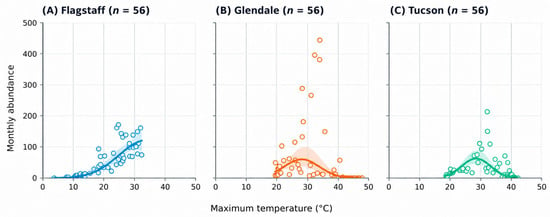
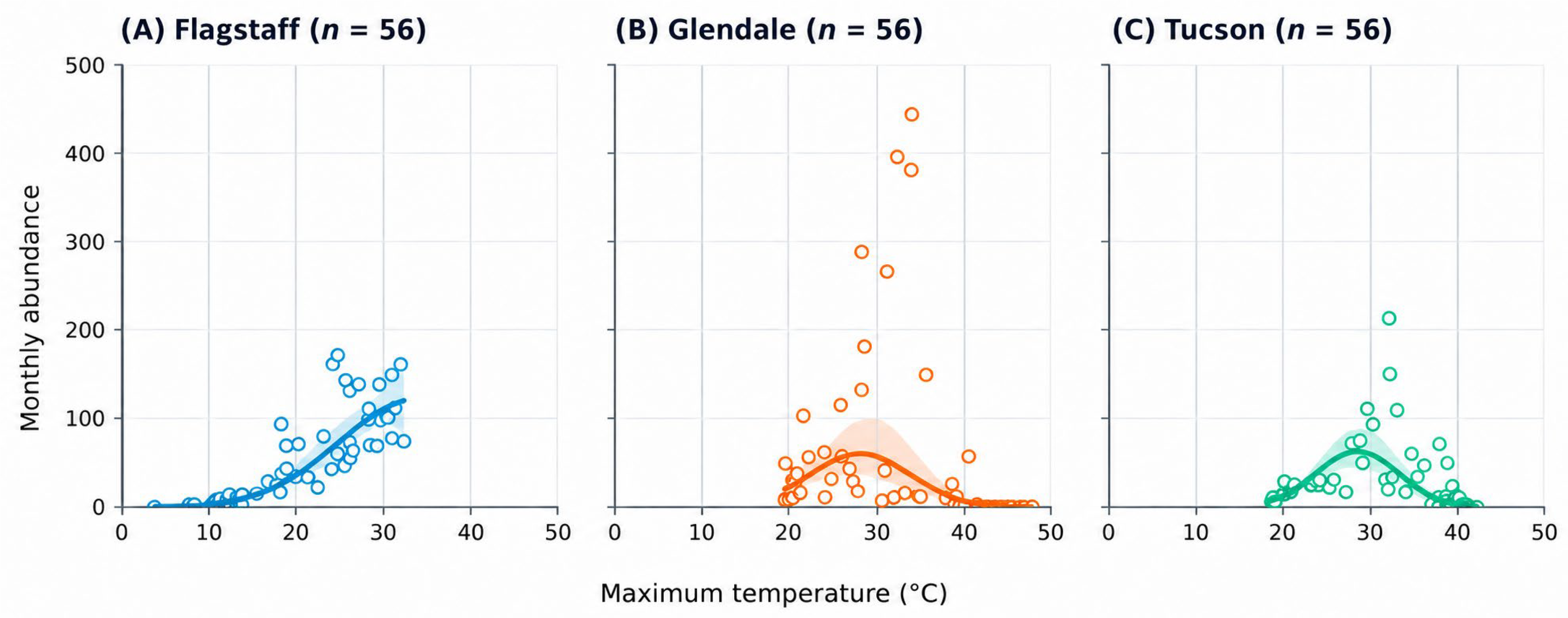
Associations between calliphorid abundance and environmental conditions were examined descriptively. Monthly abundance was plotted against trap-day maximum temperature separately for each sampling site. Quadratic curves were fitted to ln(abundance + 1) to visualize potential nonlinear relationships and were back-transformed to the original count scale. Shaded regions represent 95% bootstrap confidence intervals. Because temperature covaried with location, season, elevation, and other environmental characteristics, these relationships were not interpreted as causal temperature effects.
2.6.5. Species-Specific Analyses
Species-specific models were restricted to taxa collected frequently enough to support reliable parameter estimation. Abundant species were analyzed using the count-modeling approach described for total abundance, with location, year, calendar month, and selected environmental variables considered as explanatory factors. Species represented by few individuals or occurring in only a small number of samples were summarized descriptively rather than modeled independently. When the same predictor was tested across the four species-specific models, the false discovery rate was controlled using the Benjamini–Hochberg procedure. Adjustments were applied separately to the four tests of calendar month, location, and year. Raw and adjusted p values are provided in Supplementary Table S2.
3. Results
3.1. Sampling Effort and Overall Abundance
All 168 planned sampling events were completed, comprising 56 deployments at each of the Flagstaff, Glendale, and Tucson sites; no sampling observations were classified as missing. Sampling covered May–December 2020 and complete calendar years from 2021 through 2024. No non-calliphorid insects or other arthropods were observed in the traps. A total of 7972 adult blow flies representing 11 species were included in the analyses. Total abundance was greatest in Glendale, where 3166 specimens were collected, followed by Flagstaff with 3113 specimens and Tucson with 1693 specimens (Table 1). Mean monthly abundance was similar in Glendale (56.5 ± 104.2 flies) and Flagstaff (55.6 ± 51.5 flies), but lower in Tucson (30.2 ± 40.4 flies). Abundance was highly variable among monthly samples, particularly in Glendale, where monthly counts ranged from zero to 444 flies. A matched-month Friedman test did not detect an overall difference in total abundance among the three locations (χ2 = 0.453, df = 2, p = 0.797).
Table 1.
Blow fly abundance, richness, diversity, and zero captures by location.
The Poisson model exhibited substantial overdispersion (Pearson dispersion statistic = 6.06; AIC = 1529.8). A negative-binomial model provided a substantially better fit (AIC = 1172.5; dispersion parameter = 0.097) and was therefore retained. A zero-inflated negative-binomial model produced only a small improvement in AIC (AIC = 1170.4) and estimated a zero-inflation probability of 0.011. Because this provided little evidence of a separate structural-zero process, the conventional negative-binomial model was retained for parsimony and biological interpretability. The location × month interaction was significant (likelihood-ratio χ2 = 378.299, df = 22, p < 0.001), demonstrating that seasonal abundance trajectories differed among the three sites. Year did not improve model fit (likelihood-ratio χ2 = 2.852, df = 4, p = 0.583), and its removal reduced the AIC from 1177.7 to 1172.5. Residual lag-one correlations ranged from −0.249 to 0.122 and were not significant at any site (all p ≥ 0.067); therefore, the independence correlation structure was retained. Because every Glendale observation during July–September was zero, the corresponding individual interaction coefficients approached the parameter boundary and were not interpreted separately. Instead, the interaction was evaluated using the omnibus test and the observed seasonal trajectories.
Across the four complete sampling years, total annual abundance ranged from 1656 specimens in 2023 to 1942 specimens in 2021. Totals of 1755 and 1759 specimens were recorded in 2022 and 2024, respectively. The 2020 total of 860 specimens was not directly comparable because sampling began in May.
3.2. Species Richness, Diversity, and Zero-Capture Samples
Mean monthly species richness differed significantly among locations (Friedman χ2 = 11.249, df = 2, p = 0.004). Flagstaff had the greatest mean richness at 6.38 ± 3.22 species per monthly sample, followed by Tucson at 5.02 ± 2.93 species and Glendale at 3.55 ± 2.85 species (Table 1). Diversity also differed among locations. Mean Shannon diversity was greatest in Flagstaff (1.316 ± 0.461), followed by Tucson (1.262 ± 0.623) and Glendale (0.795 ± 0.564). A significant overall location effect was detected for Shannon diversity (Friedman χ2 = 38.528, df = 2, p < 0.001). The same spatial pattern was observed for Simpson diversity, which averaged 0.649 ± 0.208 in Flagstaff, 0.618 ± 0.294 in Tucson, and 0.423 ± 0.298 in Glendale. Simpson diversity differed significantly among locations (Friedman χ2 = 46.453, df = 2, p < 0.001; Table 1). No blow flies were collected in 33 of the 168 monthly samples. The frequency of zero-capture samples differed significantly among locations (Cochran’s Q = 11.217, df = 2, p = 0.004). Glendale had the greatest number of zero-capture samples, with no calliphorids collected during 18 of 56 sampling months (32.1%). Tucson had 10 zero-capture samples (17.9%), whereas Flagstaff had five (8.9%). Holm-adjusted pairwise comparisons indicated that zero captures were more frequent in Glendale than in Flagstaff (p = 0.023) and Tucson (p = 0.023). The difference between Flagstaff and Tucson was not significant (p = 0.302).
3.3. Species Abundance and Composition
Lucilia sericata was the most abundant species, accounting for 3015 specimens and 37.8% of the total collection (Table 2). It was detected in 127 of the 168 monthly samples (75.6%). Calliphora latifrons was the second most abundant species, comprising 1809 specimens (22.7%), and occurred in 126 samples (75.0%). Phormia regina (Meigen, 1826) accounted for 1450 specimens (18.2%), whereas Lucilia mexicana Macquart, 1843, accounted for 781 specimens (9.8%). Together, these four species represented 88.5% of all specimens collected. The remaining species occurred at substantially lower abundances. Cochliomyia macellaria (Fabricius, 1775) accounted for 351 specimens (4.4%), and Calliphora coloradensis Hough, 1899, accounted for 201 specimens (2.5%). Each of the remaining five species represented approximately 1.2% or less of the total collection. These included Protophormia terraenovae (Robineau-Desvoidy, 1830) (n = 97), Lucilia cuprina (Wiedemann, 1830) (n = 80), Calliphora livida Hall, 1948 (n = 79), Chrysomya rufifacies (n = 55), and Cynomya cadaverina (n = 54; Table 2).
Table 2.
Species abundance, relative abundance, occurrence, and location-specific counts.
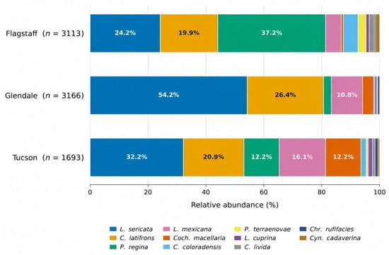
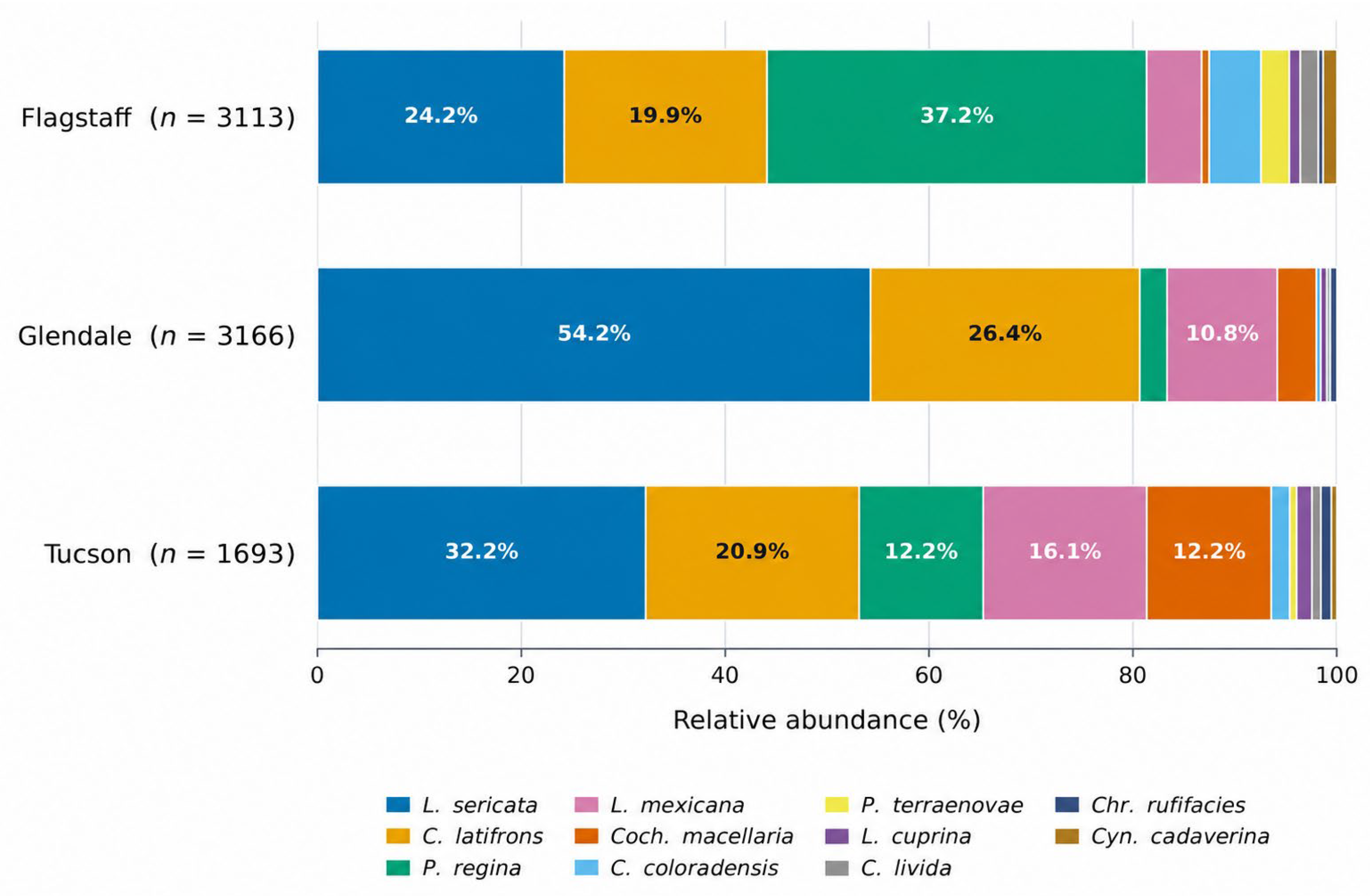
Species composition varied markedly among locations (Figure 1). The Flagstaff assemblage was dominated by Ph. regina, which accounted for 1159 specimens and 37.2% of the Flagstaff collection. L. sericata and C. latifrons represented 24.2% and 19.9%, respectively. In contrast, the Glendale assemblage was dominated by L. sericata, which accounted for 1717 specimens and 54.2% of the location total. C. latifrons represented an additional 26.4% of the Glendale collection. The Tucson assemblage was more evenly distributed, with L. sericata accounting for 32.2%, C. latifrons for 20.9%, L. mexicana for 16.1%, and both Ph. regina and C. macellaria accounting for 12.2% each. Neither Prot. terraenovae nor C. cadaverina was collected in Glendale. Monthly abundances of each species at the three sampling sites are provided in Supplementary Figure S1.
Figure 1.
Relative species composition of adult blow fly assemblages collected at the Flagstaff, Glendale, and Tucson sampling sites from May 2020 through December 2024. Bars show the percentage of specimens collected at each site attributable to each species. Species represented by at least 10 specimens at any one site were displayed individually. All 11 species met this criterion; therefore, no species were combined into an “Other” category.
Negative-binomial models fitted to the four most abundant species demonstrated significant monthly variation for L. sericata (likelihood-ratio χ2 = 57.057, df = 11, adjusted p < 0.001), C. latifrons (χ2 = 63.983, df = 11, adjusted p < 0.001), Ph. regina (χ2 = 44.841, df = 11, adjusted p < 0.001), and L. mexicana (χ2 = 45.031, df = 11, adjusted p < 0.001). Location was significantly associated with the abundance of L. sericata (χ2 = 7.275, df = 2, adjusted p = 0.035), C. latifrons (χ2 = 17.839, df = 2, adjusted p < 0.001), and Ph. regina (χ2 = 62.802, df = 2, adjusted p < 0.001), but not L. mexicana (χ2 = 1.155, df = 2, adjusted p = 0.561). No significant year effect was detected for any of the four species during the complete sampling years of 2021–2024 (all adjusted p ≥ 0.898). Raw and adjusted p values are presented in Supplementary Table S1.
3.4. Monthly Patterns in Abundance
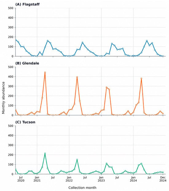
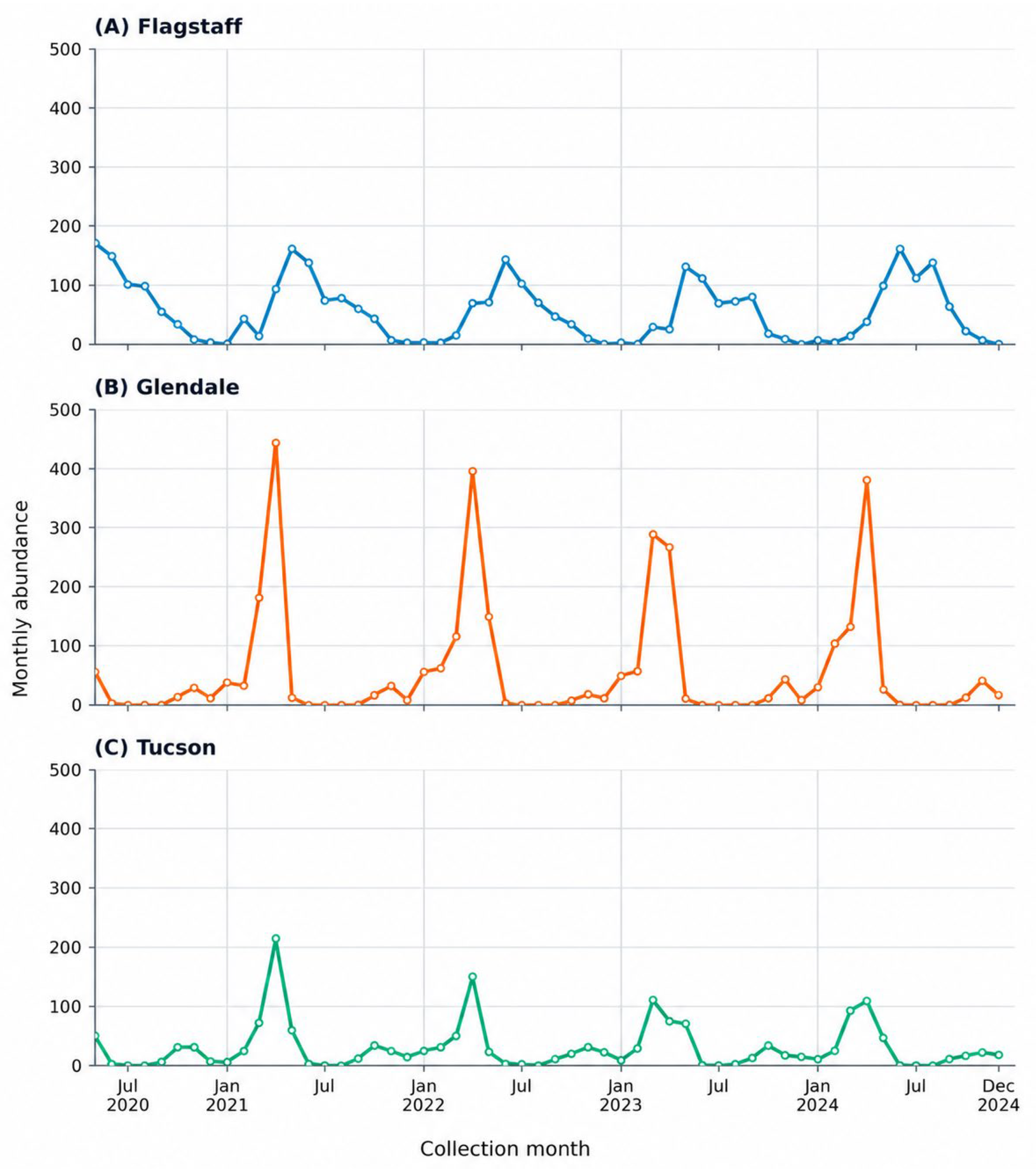
Although the matched-month Friedman test did not detect an overall difference in abundance among sites when averaged across the study period, the significant location × month interaction demonstrated that seasonal abundance trajectories differed among sites (Figure 2). Flagstaff exhibited a broad warm-season activity period, with the greatest mean abundance during May and June and relatively high captures continuing through August. Abundance subsequently declined through autumn and was lowest during winter. The largest single collection in Flagstaff occurred in May 2020, when 171 flies were collected. In contrast, Glendale exhibited a concentrated spring peak. Abundance increased during February and March, peaked in April, and declined sharply by June. No blow flies were collected in Glendale during July, August, or September in any sampling year. The largest collection recorded during the study occurred in Glendale in April 2021 and contained 444 specimens. Tucson exhibited a similar but less pronounced spring-centered trajectory, with abundance greatest during March and April before declining during May and June. Captures were generally low or absent during the hottest summer months but increased again during autumn. The largest Tucson collection occurred in April 2021 and contained 213 specimens (Figure 2).
Figure 2.
Monthly blow fly abundance at the Flagstaff, Glendale, and Tucson sampling locations from May 2020 through December 2024. Each point represents one location-month sampling unit. Note that sampling in 2020 began in May.
3.5. Environmental Conditions and Abundance
Environmental conditions differed substantially among locations (Table 3). Flagstaff was the coolest sampling location, with a mean maximum temperature of 20.2 ± 7.8 °C and a mean minimum temperature of 0.2 ± 7.7 °C. Glendale had the greatest mean maximum temperature (33.8 ± 9.1 °C) and mean minimum temperature (17.5 ± 8.0 °C), followed by Tucson, where the corresponding values were 31.9 ± 7.8 °C and 14.2 ± 8.1 °C. The highest recorded maximum temperature was 47.8 °C in Glendale, compared with 42.3 °C in Tucson and 32.3 °C in Flagstaff. Mean relative humidity was greatest in Flagstaff (42.8 ± 10.2%) and lower in Tucson (33.3 ± 9.4%) and Glendale (31.3 ± 9.1%; Table 3). Descriptive relationships between abundance and maximum temperature were nonlinear and varied among locations (Figure 3). Abundance generally increased from low to intermediate maximum temperatures but declined at the upper end of the temperature range. This decline was especially apparent in Glendale and Tucson, where samples collected during the highest-temperature periods frequently contained few or no blow flies. In Flagstaff, the greatest abundances occurred under comparatively moderate maximum temperatures. The curves and confidence intervals presented in Figure 3 are descriptive; formal inference regarding temperature effects should be based on the final negative-binomial environmental model.
Table 3.
Environmental conditions by location.
Figure 3.
Association between monthly blow fly abundance and maximum temperature at the Flagstaff, Glendale, and Tucson sampling locations. Points represent individual location-month samples. Solid lines represent descriptive quadratic fits to log-transformed abundance [ln(abundance + 1)] back-transformed to the original count scale; shaded regions indicate 95% bootstrap confidence intervals.
4. Discussion
Adult blow fly seasonality, diversity, and composition differed among the three Arizona sampling sites despite no significant difference in mean monthly abundance. Glendale exhibited a concentrated spring activity period and frequent zero captures, Flagstaff supported a broader warm-season assemblage, and Tucson showed an intermediate pattern. Overall abundance alone therefore did not adequately characterize these communities.
This study addresses a geographic gap between surveys in southern, central, and northwestern Arizona [7,9,10]. However, one fixed site and one trap per monthly event provided temporal replication but no within-location spatial replication. The findings therefore characterize adult activity at three fixed sites rather than citywide populations or carrion colonization. Although geographic variation in blow fly communities has been associated with elevation, ecoregion, vegetation, and urbanization [5,14,15], and Flagstaff’s comparatively diverse assemblage is consistent with previous observations from northwestern Arizona [10], these factors were confounded with location and could not be evaluated independently.
The strongest seasonal contrast was between extended warm-season activity at Flagstaff and the absence of Glendale captures during July–September, consistent with reduced abundance during extreme heat previously reported in Phoenix [9]. Abundance generally increased from low to intermediate temperatures before declining at the highest temperatures. Temperature can affect blow fly flight, carrion attendance, oviposition, development, and survival [6,16,17], and oviposition by Lucilia sericata and Phormia regina does not increase indefinitely with temperature [6]. Nevertheless, these relationships were descriptive because temperature covaried with location, season, and other environmental factors.
These findings have potential forensic relevance by providing regional and seasonal context for species recovered during casework. Reduced captures during extreme heat identify conditions under which delayed colonization may warrant consideration, but bait traps do not measure oviposition or successful colonization. Absence from a trap therefore does not demonstrate that carrion colonization ceased; carcass-based studies are required to test this possibility. Consider a July death investigation near the Glendale sampling site in which recently deposited blow fly larvae are recovered. Without regional baseline data, an investigator might assume that high temperatures promoted rapid colonization. An investigator familiar with this study would recognize that no flies were captured at the Glendale site during July–September and might therefore evaluate delayed colonization by examining scene access and temperature records. These data cannot establish or quantify a colonization delay, but they identify a locally supported possibility and encourage appropriate reporting of uncertainty.
No species was a consistent indicator across all sites and seasons. Lucilia sericata dominated the low-desert collections, consistent with previous Phoenix findings [9], but varied seasonally. Calliphora latifrons occurred at all three sites and in 75% of monthly samples and has been reported as dominant in Phoenix [9] and northwestern Arizona [10]. In contrast, Ph. regina was associated primarily with Flagstaff, while Lucilia mexicana occurred broadly but varied seasonally. Following its first Arizona record in the northwest [10], recovery of Cynomya cadaverina at Flagstaff and Tucson suggests a broader distribution than previously documented. These patterns favor site- and season-specific baselines over a single statewide indicator. Chrysomya rufifacies was the only collected species recognized as a relatively recent North American introduction. It was first confirmed in Arizona by Baumgartner [8], with its northernmost state record later reported by Kahler and Weidner [10]. Although it represented less than 1% of specimens, its larvae can prey on other carrion-associated larvae, including Cochliomyia macellaria, and alter carrion communities [18]. Its occurrence at all three sites supports continued monitoring through spatially replicated sampling.
Annual abundance was approximately 15% lower in 2023 than in 2021, although no significant year effect was detected for the four dominant species. This difference may reflect variation in weather, resource availability, or sampling conditions, but its cause could not be determined from the observational design.
Several limitations affect interpretation. One fixed trap per site provided temporal but not spatial replication and may have introduced site-specific effects. Baited traps measure adult presence and attraction rather than colonization, and species may respond differently to traps and remains [19]. Bait warming or desiccation may also have reduced summer captures. Trap- and net-collected specimens were not recorded separately, and monthly sampling could not resolve short-term weather effects. Future studies should incorporate replicated sites, separate and standardized collection methods, and carcass-based sampling.
5. Conclusions
This study provides a contemporary multiyear baseline for adult blow fly presence and seasonal activity at three fixed Arizona sites. The findings demonstrate that species occurrence and seasonal expectations observed at one site should not be extrapolated automatically to other locations. Reduced captures during extreme desert heat suggest suppression of adult activity or attraction to bait, but they do not establish delayed or absent carrion colonization. Because the design provided temporal but not within-region spatial replication, the results characterize the sampled sites rather than entire metropolitan regions. The recovery of Cynomya cadaverina at Flagstaff and Tucson suggests that this species may occur more broadly in Arizona than previously documented. Replicated regional surveys, standardized collection methods, carcass-based studies, and locally derived developmental data are needed to determine the generality and forensic significance of the patterns observed here.
Supplementary Materials
The following supporting information can be downloaded at: https://www.mdpi.com/article/10.3390/insects17111207/s1, Figure S1: Mean monthly abundance of adult blow fly species collected in Flagstaff, Glendale, and Tucson, Arizona, from May 2020 through December 2024; Table S1: Likelihood-ratio tests and Benjamini–Hochberg-adjusted p values from negative-binomial models of the four most abundant blow fly species.
Author Contributions
Conceptualization, J.J.P.; methodology, J.J.P., S.W. and K.M.; formal analysis, J.J.P., S.W., K.M., G.F. and A.B.; investigation, J.J.P., S.W., K.M., G.F. and A.B.; data curation, J.J.P. and S.W.; writing—original draft preparation, J.J.P.; writing—review and editing, J.J.P., S.W., K.M., G.F. and A.B.; visualization, J.J.P. and S.W.; supervision, J.J.P. All authors have read and agreed to the published version of the manuscript.
Funding
This research received no external funding.
Data Availability Statement
The original contributions presented in this study are included in the article and supplementary material. Further inquiries can be directed to the corresponding author.
Conflicts of Interest
The authors declare no conflicts of interest.
References
- Greenberg, B. Flies as forensic indicators. J. Med. Entomol. 1991, 28, 565–577. [Google Scholar] [CrossRef] [Scilit] [PubMed]
- Amendt, J.; Campobasso, C.P.; Gaudry, E.; Reiter, C.; LeBlanc, H.N.; Hall, M.J.R. Best practice in forensic entomology—Standards and guidelines. Int. J. Leg. Med. 2007, 121, 90–104. [Google Scholar] [CrossRef] [Scilit] [PubMed]
- Amendt, J.; Richards, C.S.; Campobasso, C.P.; Zehner, R.; Hall, M.J.R. Forensic entomology: Applications and limitations. Forensic Sci. Med. Pathol. 2011, 7, 379–392. [Google Scholar] [CrossRef] [Scilit] [PubMed]
- Zabala, J.; Díaz, B.; Saloña-Bordas, M.I. Seasonal blowfly distribution and abundance in fragmented landscapes. Is it useful in forensic inference about where a corpse has been decaying? PLoS ONE 2014, 9, e99668. [Google Scholar] [CrossRef] [Scilit] [PubMed]
- Weidner, L.M.; Jennings, D.E.; Tomberlin, J.K.; Hamilton, G.C. Seasonal and geographic variation in biodiversity of forensically important blow flies (Diptera: Calliphoridae) in New Jersey, USA. J. Med. Entomol. 2015, 52, 937–946. [Google Scholar] [CrossRef] [Scilit] [PubMed]
- Hans, K.R.; LeBouthillier, R.; VanLaerhoven, S.L. Effect of temperature on oviposition behavior and egg load of blow flies (Diptera: Calliphoridae). J. Med. Entomol. 2019, 56, 441–447. [Google Scholar] [CrossRef] [Scilit] [PubMed]
- Deonier, C.C. Seasonal abundance and distribution of certain blowflies in southern Arizona and their economic importance. J. Econ. Entomol. 1942, 35, 65–70. [Google Scholar] [CrossRef] [Scilit]
- Baumgartner, D.L. The hairy maggot blow fly, Chrysomya rufifacies (Macquart), confirmed in Arizona. J. Entomol. Sci. 1986, 21, 130–132. [Google Scholar] [CrossRef] [Scilit]
- Meeds, A.W.; Rusch, T.W.; Falcone, D.L.; Weidner, L.M. A survey of blow fly (Diptera: Calliphoridae) populations in Phoenix, Arizona. Front. Ecol. Evol. 2023, 11, 1158347. [Google Scholar] [CrossRef] [Scilit]
- Kahler, G.V.; Weidner, L.M. Effects of elevation, season and bait type on assemblage of forensically relevant blow flies (Diptera: Calliphoridae) in contrasting habitats of northwestern Arizona. Med. Vet. Entomol. 2026, 40, 647–658. [Google Scholar] [CrossRef] [Scilit] [PubMed]
- Farinha, A.; Dourado, C.G.; Centeio, N.; Oliveira, A.R.; Dias, D.; Rebelo, M.T. Small bait traps as accurate predictors of dipteran early colonizers in forensic studies. J. Insect Sci. 2014, 14, 77. [Google Scholar] [CrossRef] [Scilit] [PubMed]
- Marshall, S.A.; Whitworth, T.; Roscoe, L. Blow flies (Diptera: Calliphoridae) of eastern Canada with a key to Calliphoridae subfamilies and genera of eastern North America, and a key to the eastern Canadian species of Calliphorinae, Luciliinae and Chrysomyiinae. Can. J. Arthropod Identif. 2011, 11, 1–93. [Google Scholar] [CrossRef]
- Forensic Entomology: The Utility of Arthropods in Legal Investigations, 3rd ed.; Byrd, J.H., Tomberlin, J.K., Eds.; CRC Press: Boca Raton, FL, USA, 2020. [Google Scholar]
- Brundage, A.; Bros, S.; Honda, J.Y. Seasonal and habitat abundance and distribution of some forensically important blow flies (Diptera: Calliphoridae) in central California. Forensic Sci. Int. 2011, 212, 115–120. [Google Scholar] [CrossRef] [Scilit] [PubMed]
- Cumming, R.T.; Dufek, M.I. Assemblages of necrophagous blow flies (Diptera: Calliphoridae) in four contrasting ecoregions of Los Angeles County, California, United States. J. Med. Entomol. 2021, 58, 2236–2246. [Google Scholar] [CrossRef] [Scilit] [PubMed]
- Mohr, R.M.; Tomberlin, J.K. Environmental factors affecting early carcass attendance by four species of blow flies (Diptera: Calliphoridae) in Texas. J. Med. Entomol. 2014, 51, 702–708. [Google Scholar] [CrossRef] [Scilit] [PubMed]
- Lutz, L.; Verhoff, M.A.; Amendt, J. Environmental factors influencing flight activity of forensically important female blow flies in Central Europe. Int. J. Leg. Med. 2019, 133, 1267–1278. [Google Scholar] [CrossRef] [Scilit] [PubMed]
- Wells, J.D.; Greenberg, B. Interaction between Chrysomya rufifacies and Cochliomyia macellaria (Diptera: Calliphoridae): The possible consequences of an invasion. Bull. Entomol. Res. 1992, 82, 133–137. [Google Scholar] [CrossRef] [Scilit]
- Weidner, L.M.; Gemmellaro, M.D.; Tomberlin, J.K.; Hamilton, G.C. Evaluation of bait traps as a means to predict initial blow fly (Diptera: Calliphoridae) communities associated with decomposing swine remains in New Jersey, USA. Forensic Sci. Int. 2017, 278, 95–100. [Google Scholar] [CrossRef] [Scilit] [PubMed]

Disclaimer/Publisher’s Note: The statements, opinions and data contained in all publications are solely those of the individual author(s) and contributor(s) and not of MDPI and/or the editor(s). MDPI and/or the editor(s) disclaim responsibility for any injury to people or property resulting from any ideas, methods, instructions or products referred to in the content. |
© 2026 by the authors. Licensee MDPI, Basel, Switzerland. This article is an open access article distributed under the terms and conditions of the Creative Commons Attribution (CC BY) license.